Embed Size (px)
Citation preview

HAL Id: tel-01686395https://tel.archives-ouvertes.fr/tel-01686395
Submitted on 17 Jan 2018
HAL is a multi-disciplinary open accessarchive for the deposit and dissemination of sci-entific research documents, whether they are pub-lished or not. The documents may come fromteaching and research institutions in France orabroad, or from public or private research centers.
L’archive ouverte pluridisciplinaire HAL, estdestinée au dépôt et à la diffusion de documentsscientifiques de niveau recherche, publiés ou non,émanant des établissements d’enseignement et derecherche français ou étrangers, des laboratoirespublics ou privés.
International trade, trade costs and quality of tradedcommodities
Viola Lamani
To cite this version:Viola Lamani. International trade, trade costs and quality of traded commodities. Economics andFinance. Université de Bordeaux, 2017. English. �NNT : 2017BORD0746�. �tel-01686395�
THESE PRESENTEE
POUR OBTENIR LE GRADE DE
DOCTEUR DE
L’UNIVERSITE DE BORDEAUX
ECOLE DOCTORALE ENTREPRISE, ECONOMIE, SOCIETE (ED. 42)
SPECIALITE SCIENCES ECONOMIQUES
Par Viola LAMANI
International Trade, Trade Costs andQuality of Traded Commodities
Commerce International, Couts a l’Echange et Qualite des
Produits Echanges
Sous la direction de :
M. Antoine BOUET et Mme Charlotte EMLINGER
Soutenue le 24 Novembre 2017
Membres du jury :
M. FONTAGNE, Lionel
Professeur des Universites, Universite Paris 1 Pantheon-Sorbonne, President
M. ANDERSON, Kym
Professor of Economics, University of Adelaide, Rapporteur
Mme DISDIER, Anne-Celia
Directrice de Recherche, INRA, Rapporteure
M. STORCHMANN, Karl
Clinical Professor of Economics, New York University, Examinateur


Acknowledgments
First and foremost, I would like to thank my PhD supervisors: Antoine Bouet and Char-
lotte Emlinger. Your careful examinations and invaluable comments have greatly con-
tributed to this dissertation. Thanks to your unfaltering efforts, this work has yielded
a co-authored paper that has been published. Professor Bouet, you have supported me
since the beginning of this journey, and pushed me to always do my best. You first gave
me a “taste for research” as my professor of economic modeling and have continued to
inspire me during the past four years. Charlotte, you took me in as an intern at CEPII
and worked with me with great patience every day during that month. Since then, you
have continuously helped me with this dissertation and I am very excited about what
the future holds for our paper. Your openness, kindness and good humor have been a
comfort to me, even in my moments of doubt. Both of you have helped shape me into
the researcher that I am today.
I would also like to thank the members of the jury: Kym Anderson, Anne-Celia Disdier,
Lionel Fontagne and Karl Storchmann who have very kindly accepted to examine this
work. I have already had the opportunity to present in front of them preliminary versions
of the papers in this dissertation and have greatly benefited from their many helpful com-
ments.
I am very grateful to the Bureau National Interprofessionnel du Cognac for helping us
from the start with the constitution of the database on Cognac exports, as well as for
providing constant attention and making interesting suggestions to this work. In partic-
ular, I thank Janine Bretagne, Christakis Christodoulou, Nadia Folio, Stephane Feuillet,
Sebastien Freulon, Lionel Lalague, and Catherine Lepage. I offer special thanks to Xavier
Pichot from the ITC for providing us with the data on customs protections and Houssein
Guimbard from CEPII for providing us with the data from MAcMap.
I have also had the amazing opportunity to discuss my research, at the very beginning,
with Daniel Bernhofen who gave me great ideas and directions for my work and very
kindly provided us with the data on containerization.
iii

The third chapter of this dissertation would not have been written without the help and
efforts of Julien Berthoumieu. Julien, you have demonstrated great patience toward me
and I am inspired by your work diligence. It has also been a pleasure working with you
for the online course. Our thought-provoking discussions (even those not related to R&D)
have always been a source of excitement, even when they led to heated debates!
This dissertation has benefited greatly from helpful suggestions from participants in
LAREFI, GREThA and CEPII seminars; AAWE, ETSG, IATRC, MAD and SFER con-
ferences. In particular I would like to thank: Tanguy Bernard, Sophie Brana, Jason Brent,
Jean-Marie Cardebat, Angela Cheptea, Matthieu Clement, Karine Latouche, Thierry
Mayer, Eric Rougier, Dominique Van der Mensbrugghe, and Anne-Gael Vaubourg. I
would also like to offer special thanks to Matthieu Crozet, Sebastien Jean, and Vincent
Vicard for their careful examination of the paper related to the Cognac quality mix.
Many thanks go to Cristina Badarau and Michel Dupuy for trusting me with their travaux
diriges and helping me to have a very pleasant teaching experience.
My research started in LAREFI and then continued in GREThA, therefore I would like
to thank their respective directors, Jean-Marie Cardebat and Marc-Alexandre Senegas for
their support.
One of the main reasons that I am able today to write these pages of acknowledgments,
sitting at my office in Bordeaux, is because of my family. Laurina, Mami, Babi, Mama
Eko: a thank you would be far from enough for your unconditional love and support.
Nine years ago, you gave me the opportunity to study in France and have never ceased
to watch over me. You have even shared my passion of Cognac and have a very good
grasp of the Alchian and Allen effect! We have always discussed our teaching and research
experiences and I will always look up to you. I share a particular bond with you Laurina,
thank you for always comforting me when I become a ball of stress!
During these years, I have crossed paths with many amazing people. I would like to thank
in general all the PhD students of LAREFI and GREThA. In particular: Louis, Ibrahima,
Thomas you were the first to welcome me in our office in Larefi when I started my PhD.
We have had countless discussions and have shared many laughs (even cries a few times).
A heartfelt thanks also goes to Katia, Linda, Robin, Marine, Francois V, Irena, Laurent,
Louai, Alexandra, Clement. Jeanne and Bao, my friends and current office colleagues:
thank you for the discussions, but most of all for the laughs and fun - you made it so
easy especially these past few weeks. To Lionel: thank you for carefully proof-reading my
conclusion and I hope I have not “traumatized” you at the beginning of your PhD journey.
iv

Thank you Genevieve for your corrections and for always being open to discussions.
To Onigiri: we will be going our separate ways but you have demonstrated unconditional
support for my work. Thank you! To my dear Sunny: a ray of light - I can’t begin to
describe the help and joy you have brought me (thank you of course for the corrections).
Thank you Dan, Nico Y, Pierre, Thibaud, Nico B, Francois, Samuel, Manu for many
discussions, for sharing meals (and drinks) and many dances together! Also, thank you
Pierre and Riana for your great help with the French summary! A big up to Lucile,
Marjorie, Jeremy, Fadoua, Pauline: you rule!
Finally, to that special someone: it started as the “pilot” of a TV series that will hopefully
have many seasons. I am excited for the future and I owe it to you for encouraging me!
v


Contents
0 General Introduction 1
0.1 Trade Costs: A State of Evidence . . . . . . . . . . . . . . . . . . . . . . . 3
0.2 Quality: Definition and Measurement . . . . . . . . . . . . . . . . . . . . . 8
0.3 How Do Trade Costs Affect Quality? . . . . . . . . . . . . . . . . . . . . . 10
0.4 An In-Depth View of the Dissertation . . . . . . . . . . . . . . . . . . . . . 12
1 Determinants of Cognac Exports 15
1.1 Introduction . . . . . . . . . . . . . . . . . . . . . . . . . . . . . . . . . . . 15
1.2 Review of Literature . . . . . . . . . . . . . . . . . . . . . . . . . . . . . . 16
1.3 Data and Descriptive Statistics . . . . . . . . . . . . . . . . . . . . . . . . 19
1.3.1 Cognac Sales and Export . . . . . . . . . . . . . . . . . . . . . . . . 19
1.3.2 The Protection Database . . . . . . . . . . . . . . . . . . . . . . . . 23
1.4 Econometric Estimation . . . . . . . . . . . . . . . . . . . . . . . . . . . . 25
1.4.1 Empirical Strategy and Data . . . . . . . . . . . . . . . . . . . . . . 25
1.4.2 Results . . . . . . . . . . . . . . . . . . . . . . . . . . . . . . . . . . 27
1.4.3 Discussion . . . . . . . . . . . . . . . . . . . . . . . . . . . . . . . . 31
1.4.4 Robustness tests . . . . . . . . . . . . . . . . . . . . . . . . . . . . 32
1.5 Conclusion . . . . . . . . . . . . . . . . . . . . . . . . . . . . . . . . . . . . 38
1.A Income Disparity and the Gravity Equation . . . . . . . . . . . . . . . . . 45
1.B Determinants of Export Unit Values . . . . . . . . . . . . . . . . . . . . . 49
2 Cognac Quality and Trade Costs 51
2.1 Introduction . . . . . . . . . . . . . . . . . . . . . . . . . . . . . . . . . . . 51
2.2 The Alchian and Allen Effect . . . . . . . . . . . . . . . . . . . . . . . . . 54
2.2.1 Theoretical Framework . . . . . . . . . . . . . . . . . . . . . . . . . 54
2.2.2 Extensions . . . . . . . . . . . . . . . . . . . . . . . . . . . . . . . . 56
2.2.3 Empirical Verification . . . . . . . . . . . . . . . . . . . . . . . . . 57
2.3 Cognac Quality Designations . . . . . . . . . . . . . . . . . . . . . . . . . . 58
2.3.1 Qualities Depending on the Ageing System . . . . . . . . . . . . . . 58
2.3.2 An Original Dataset . . . . . . . . . . . . . . . . . . . . . . . . . . 59
vii

CONTENTS
2.4 Distance, Tariffs and Quality Mix . . . . . . . . . . . . . . . . . . . . . . . 61
2.4.1 Stylized Facts . . . . . . . . . . . . . . . . . . . . . . . . . . . . . . 61
2.4.2 Empirical Strategy and Data . . . . . . . . . . . . . . . . . . . . . . 63
2.4.3 Results . . . . . . . . . . . . . . . . . . . . . . . . . . . . . . . . . . 64
2.5 Containerization and Quality Mix . . . . . . . . . . . . . . . . . . . . . . . 67
2.5.1 Stylized Facts on Containerization . . . . . . . . . . . . . . . . . . . 67
2.5.2 Empirical Strategy and Data . . . . . . . . . . . . . . . . . . . . . . 70
2.5.3 Results . . . . . . . . . . . . . . . . . . . . . . . . . . . . . . . . . . 71
2.6 Conclusion . . . . . . . . . . . . . . . . . . . . . . . . . . . . . . . . . . . . 74
2.A General Framework: Mathematical Proofs . . . . . . . . . . . . . . . . . . 75
2.A.1 The Alchian and Allen Effect in a Two-Good World . . . . . . . . . 75
2.A.2 The Alchian and Allen Effect in a Three-Good World . . . . . . . . 76
2.B Stylized facts: Main Markets . . . . . . . . . . . . . . . . . . . . . . . . . . 78
2.C Distance, Tariffs and Quality Mix: An Additional Test . . . . . . . . . . . 80
2.D Containerization: Databases . . . . . . . . . . . . . . . . . . . . . . . . . . 81
2.E Containerization and Quality Mix: An Additional Test . . . . . . . . . . . 84
3 Product R&D and Policy Instruments 85
3.1 Introduction . . . . . . . . . . . . . . . . . . . . . . . . . . . . . . . . . . . 85
3.2 Review of Literature . . . . . . . . . . . . . . . . . . . . . . . . . . . . . . 88
3.3 General Framework . . . . . . . . . . . . . . . . . . . . . . . . . . . . . . . 90
3.3.1 Successful R&D . . . . . . . . . . . . . . . . . . . . . . . . . . . . . 93
3.3.2 Unsuccessful R&D . . . . . . . . . . . . . . . . . . . . . . . . . . . 94
3.3.3 Choice of R&D Investment . . . . . . . . . . . . . . . . . . . . . . . 95
3.4 Equilibrium with Linear Demand Functions . . . . . . . . . . . . . . . . . 96
3.5 The Implementation of Two Traditional Policy Instruments . . . . . . . . . 98
3.5.1 A Specific Import Tariff . . . . . . . . . . . . . . . . . . . . . . . . 99
3.5.2 An Import Quota . . . . . . . . . . . . . . . . . . . . . . . . . . . . 101
3.6 A Quality Standard . . . . . . . . . . . . . . . . . . . . . . . . . . . . . . . 105
3.7 Welfare Analysis . . . . . . . . . . . . . . . . . . . . . . . . . . . . . . . . 106
3.7.1 General Framework under Free Trade . . . . . . . . . . . . . . . . . 107
3.7.2 Discussion . . . . . . . . . . . . . . . . . . . . . . . . . . . . . . . . 107
3.8 A Non-Prohibitive Quality Standard . . . . . . . . . . . . . . . . . . . . . 110
3.9 Concluding Remarks . . . . . . . . . . . . . . . . . . . . . . . . . . . . . . 112
3.A Impact of “At-the-Border” Policy Instruments on Expected Consumer Sur-
plus . . . . . . . . . . . . . . . . . . . . . . . . . . . . . . . . . . . . . . . 115
3.B Welfare Analysis . . . . . . . . . . . . . . . . . . . . . . . . . . . . . . . . 116
3.C Welfare Analysis with the Non-Prohibitive Quality Standard . . . . . . . . 117
viii

CONTENTS
General Conclusion 119
A Global Appendix 123
A.1 Categorizing Trade Costs . . . . . . . . . . . . . . . . . . . . . . . . . . . . 124
A.2 Quality: A Multidimensional Concept . . . . . . . . . . . . . . . . . . . . . 125
A.3 Compiling the Database on Cognac Exports from 1967 to 2013 . . . . . . . 127
A.3.1 Collecting the Data . . . . . . . . . . . . . . . . . . . . . . . . . . . 127
A.3.2 The Geographic Coverage of the Database . . . . . . . . . . . . . . 127
A.3.3 From the French Franc to the Euro . . . . . . . . . . . . . . . . . . 128
A.3.4 From 6 to 3 Qualities of Cognac . . . . . . . . . . . . . . . . . . . . 128
A.4 Cognac Shipments from 1967 to 2013: Stylized Facts . . . . . . . . . . . . 129
Resume en Francais 135
Bibliography 145
ix


List of Tables
1.1 Worldwide Customs Protection on Cognac: Statistics for more than 100
Importing Countries, 1996-2013 . . . . . . . . . . . . . . . . . . . . . . . . 24
1.2 Baseline Estimation: Heckman Procedure . . . . . . . . . . . . . . . . . . . 29
1.3 Baseline Estimation: IV Probit . . . . . . . . . . . . . . . . . . . . . . . . 30
1.4 Robustness Check I: Alternative Customs Protection Measure: Heckman
Procedure . . . . . . . . . . . . . . . . . . . . . . . . . . . . . . . . . . . . 33
1.5 Robustness Check I: Alternative Customs Protection Measure: IV Probit . 34
1.6 Robustness Check II: Adding Continents’ FE: Heckman Procedure . . . . . 35
1.7 Robustness Check II: Adding Continents’ FE: IV Probit . . . . . . . . . . 36
1.8 Robustness Check IIIa: Alternative Estimation Method: PPML . . . . . . 37
1.9 Robustness Check IIIb: Alternative Estimation Method: EK Tobit . . . . . 38
1.10 Summary Statistics . . . . . . . . . . . . . . . . . . . . . . . . . . . . . . . 42
1.11 List of Cognac Importing Countries in 2013 . . . . . . . . . . . . . . . . . 43
1.12 List of Muslim-Majority Countries with their Dates of Information accord-
ing to the CIA Factbook . . . . . . . . . . . . . . . . . . . . . . . . . . . . 44
1.13 Summary Statistics: Full Sample vs. Gini Sample . . . . . . . . . . . . . . 45
1.14 Including the Gini Index: Intensive Margin (OLS) . . . . . . . . . . . . . . 46
1.15 Heckman Procedure with Lagged Customs Duties . . . . . . . . . . . . . . 47
1.16 List of Countries by Continents . . . . . . . . . . . . . . . . . . . . . . . . 48
1.17 OLS Estimation of the Determinants of Export Unit Values . . . . . . . . 49
2.1 OLS Estimation: Share of XO in Total Cognac Exports, 1996-2013 . . . . 65
2.2 OLS Estimation: XO Relative Export Price, 1996-2013 . . . . . . . . . . . 66
2.3 OLS Estimation: Share of XO in Total Cognac Exports, 1969-2013 . . . . 72
2.4 OLS Estimation: XO Relative Export Price, 1969-2013 . . . . . . . . . . . 73
2.5 Descriptive Statistics - Share of XO in Imports of Main Markets . . . . . . 78
2.6 Descriptive Statistics - Share of VS in Imports of Main Markets . . . . . . 78
2.7 Alternative Estimation Method: PPML, 1996-2013 . . . . . . . . . . . . . 80
2.8 Adoption of Containerization (First Port Containerized) by Cognac Im-
porting Countries . . . . . . . . . . . . . . . . . . . . . . . . . . . . . . . . 81
xi
LIST OF TABLES
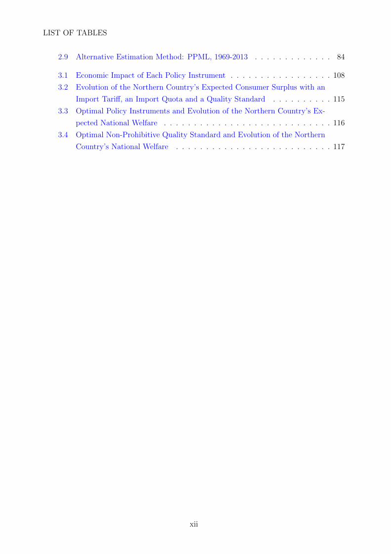
2.9 Alternative Estimation Method: PPML, 1969-2013 . . . . . . . . . . . . . 84
3.1 Economic Impact of Each Policy Instrument . . . . . . . . . . . . . . . . . 108
3.2 Evolution of the Northern Country’s Expected Consumer Surplus with an
Import Tariff, an Import Quota and a Quality Standard . . . . . . . . . . 115
3.3 Optimal Policy Instruments and Evolution of the Northern Country’s Ex-
pected National Welfare . . . . . . . . . . . . . . . . . . . . . . . . . . . . 116
3.4 Optimal Non-Prohibitive Quality Standard and Evolution of the Northern
Country’s National Welfare . . . . . . . . . . . . . . . . . . . . . . . . . . 117
xii
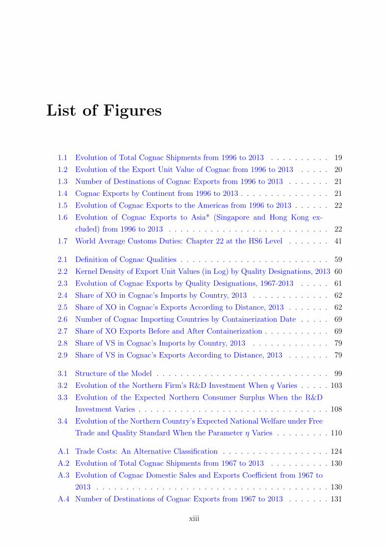
List of Figures
1.1 Evolution of Total Cognac Shipments from 1996 to 2013 . . . . . . . . . . 19
1.2 Evolution of the Export Unit Value of Cognac from 1996 to 2013 . . . . . 20
1.3 Number of Destinations of Cognac Exports from 1996 to 2013 . . . . . . . 21
1.4 Cognac Exports by Continent from 1996 to 2013 . . . . . . . . . . . . . . . 21
1.5 Evolution of Cognac Exports to the Americas from 1996 to 2013 . . . . . . 22
1.6 Evolution of Cognac Exports to Asia* (Singapore and Hong Kong ex-
cluded) from 1996 to 2013 . . . . . . . . . . . . . . . . . . . . . . . . . . . 22
1.7 World Average Customs Duties: Chapter 22 at the HS6 Level . . . . . . . 41
2.1 Definition of Cognac Qualities . . . . . . . . . . . . . . . . . . . . . . . . . 59
2.2 Kernel Density of Export Unit Values (in Log) by Quality Designations, 2013 60
2.3 Evolution of Cognac Exports by Quality Designations, 1967-2013 . . . . . 61
2.4 Share of XO in Cognac’s Imports by Country, 2013 . . . . . . . . . . . . . 62
2.5 Share of XO in Cognac’s Exports According to Distance, 2013 . . . . . . . 62
2.6 Number of Cognac Importing Countries by Containerization Date . . . . . 69
2.7 Share of XO Exports Before and After Containerization . . . . . . . . . . . 69
2.8 Share of VS in Cognac’s Imports by Country, 2013 . . . . . . . . . . . . . 79
2.9 Share of VS in Cognac’s Exports According to Distance, 2013 . . . . . . . 79
3.1 Structure of the Model . . . . . . . . . . . . . . . . . . . . . . . . . . . . . 99
3.2 Evolution of the Northern Firm’s R&D Investment When q Varies . . . . . 103
3.3 Evolution of the Expected Northern Consumer Surplus When the R&D
Investment Varies . . . . . . . . . . . . . . . . . . . . . . . . . . . . . . . . 108
3.4 Evolution of the Northern Country’s Expected National Welfare under Free
Trade and Quality Standard When the Parameter η Varies . . . . . . . . . 110
A.1 Trade Costs: An Alternative Classification . . . . . . . . . . . . . . . . . . 124
A.2 Evolution of Total Cognac Shipments from 1967 to 2013 . . . . . . . . . . 130
A.3 Evolution of Cognac Domestic Sales and Exports Coefficient from 1967 to
2013 . . . . . . . . . . . . . . . . . . . . . . . . . . . . . . . . . . . . . . . 130
A.4 Number of Destinations of Cognac Exports from 1967 to 2013 . . . . . . . 131
xiii

LIST OF FIGURES
A.5 Cognac Exports by Continent from 1967 to 2013 . . . . . . . . . . . . . . . 131
A.6 Evolution of Cognac Exports to the Americas from 1967 to 2013 . . . . . . 133
A.7 Evolution of Cognac Exports to Asia* (Singapore and Hong Kong ex-
cluded) from 1967 to 2013 . . . . . . . . . . . . . . . . . . . . . . . . . . . 134
xiv

Chapter 0
General Introduction
The increasing integration of national economies into the international economy, also
known as globalization, is a multidimensional process, extensively studied in the economic
literature and a continuous source of debate.1 The reduction of policy-related trade bar-
riers (tariffs, quotas etc.) and/or natural trade barriers (transport costs for example) is a
key component of such a process. It leads to an increase in the flows of goods and services
across borders and may be considered as one of the driving factors and among the most
visible aspects of globalization. Indeed, according to Jacks, Meissner, and Novy’s (2010)
estimations, about 44 percent of the rise of trade observed during the first wave of glob-
alization (1870-1913) can be attributed to reductions in trade barriers. These barriers
include tariffs, transport costs and all other factors that impede international trade flows.
Their estimated decrease from 1870 to 1913 is between 10 and 16 percent.2 Meanwhile
from 1950 to 2000, the estimated decline of international trade barriers is about 16 percent
which explains 31 percent of the trade growth during this period of time (Jacks, Meissner,
and Novy, 2011).3
Despite the overall downward trend observed in the past five to six decades, barriers to
trade that impede the exchange of goods across borders, commonly known in the economic
literature as trade costs, still matter.4 According to Anderson and van Wincoop (2004)
the representative estimate of total trade costs for industrialized countries is equal to 170
percent in ad valorem equivalent. This figure can be decomposed into a 74-percent ad
1For a complete and comprehensive outlook on (economic) globalization and its pros and cons, see for
example Bhagwati (2004).2Jacks, Meissner, and Novy (2010) derive a measure for all of these barriers combined based on a
micro-founded gravity model. They have data on the US, UK, France and fifteen of their most important
trading partners.3These global trends have been confirmed in a more recent empirical study by Fouquin and Hugot
(2016) using a large database of more than 1.9 million bilateral trade observations covering the period
from 1827 to 2014.4Anderson and van Wincoop (2004) explain in detail why “trade costs matter” (p.691).
1

valorem equivalent related to international costs and a 55-percent ad valorem equivalent
related to domestic (retail and wholesale distribution) costs.5
Issues related to trade costs continue to be of great interest in macroeconomics (Obstfeld
and Rogoff, 2000) and in policy debates. More recently, following the economic crisis
of 2008-2009 and the global slow growth registered in the past years, there has been an
increase in the implementation of policy-related restrictive measures. Many governments
have questioned the benefits of trade liberalization.6 Evenett (2013) refers to this trend as
“protectionism’s quiet return”. There may indeed be reasons for concern considering, for
example that the Group of Twenty (G20)7 economies implemented 145 new protectionist
measures at the fastest pace since 2009 (21 new measures per month), from mid-October
2015 to mid-May 2016 (World Trade Organization, 2016).8
For all of these reasons, trade costs have been and still are the object of extensive and
distinguished theoretical and empirical examinations starting from their definition, their
measurement, their effects etc.9 In the abundance of the economic literature on the sub-
ject, we contribute by studying the effects of trade costs on one of the key determinants
of international trade patterns: product quality.
It is well-established in the economic literature that trade in quality-differentiated prod-
ucts10 affects many important aspects of the economy like growth and development (Gross-
man and Helpman, 1991), firms’ export success (Verhoogen, 2008) and employment and
wages (Verhoogen, 2008; Khandelwal, 2010). Theoretical research on the relationship
between quality and trade is abundant following the seminal contributions of Krugman
(1979) and Lancaster (1980), to mention only a few. However, with the exception of
Linder (1961), empirical examinations of the relevance of product quality as a driver of
international trade flows have proliferated quite recently. The main challenge of these em-
5Anderson and van Wincoop’s (2004) estimates are based on direct measures (for example, from the
Trade Analysis Information System - TRAINS database for 1999) and indirect measures inferred either
from trade volumes and/or prices.6Trade liberalization can be defined as the removal or reduction of policy-related barriers to trade in
order to achieve “freer trade”.7The Group of Twenty comprises: Australia, Brazil, Canada, China, France, Germany, India, Indone-
sia, Italy, Japan, Mexico, Russia, Saudi Arabia, South Africa, South Korea, Turkey, the United Kingdom,
the United States of America and the European Union.8According to the most recent report of the WTO on G20 trade measures (june 2017), 42 new trade-
restrictive measures were introduced between mid-October 2016 and mid-May 2017.9See for example Anderson and van Wincoop (2004) for a global review of the literature on trade
costs.10Products are differentiated by quality, or vertically-differentiated when: “[for any two distinct prod-
ucts], if they were sold at the same price, then all consumers would choose the same one (the ‘higher
quality’ product)” (Shaked and Sutton, 1987, p. 134).
2

0.1. TRADE COSTS: A STATE OF EVIDENCE
pirical analyses is related to the measurement of product quality. In the first two chapters
of this dissertation, we overcome this challenge by focusing on Cognac; a product whose
quality measure is objective and invariant over time.
In chapter three we consider the quality of a firm’s product to be directly related and
dependent on the product Research and Development (product R&D) expenditures. Our
rationale for doing this is based on Sutton (2001) who argues “What determines the
levels of attainable quality, and productivity? The list of proximate causes range from
inventiveness in finding new methods of production, to the mixture of luck and judgment
involved in successful product development” (p. 249). This product development and
attainable quality is related to product R&D investment. More precisely, it involves the
creation of new or significantly improved products. The objective of firms that engage in
this investment activity is to vertically- (quality-) differentiate their products as a means
to counter competition. R&D and innovation11 in general are among the key drivers of
competitiveness and growth (Global Competitiveness Report for 2014-2015).
In the first and second chapters of the present work we adopt an empirical
approach and concentrate on Cognac, first by studying the determinants of
its trade with an emphasis on the effects of trade costs (distance and customs
protection) and then, by analyzing the impact of trade costs on the quality
mix (i.e. the quality structure) of Cognac exports. In the third chapter, we
adopt a theoretical approach and study the impact of several policy restrictive
measures (a tariff, an import quota and a quality standard) on product R&D
investment.
Before exposing in further detail the outline of this dissertation, we first discuss trade
costs. Then we discuss the definition and measurement of a product’s quality. Finally,
we review the literature on how trade costs affect the quality of traded products.
0.1 Trade Costs: A State of Evidence
Trade costs as previously defined are obstacles to international trade flows.12 They are
highly variable in time, across countries, sectors of economies and commodities. They also
differ in nature. Different trade costs have different effects on the economy (Anderson and
van Wincoop, 2004).
11Innovation goes beyond R&D. There can be product innovation, process innovation, marketing inno-
vation and organizational innovation (OECD).12Moıse and Le Bris’ (2013) definition of trade costs is the following: “[...]the difference between the
amount of trade flows that would take place in a hypothetical ‘frictionless’ world and what is actually
observed” (p.6).
3

0.1. TRADE COSTS: A STATE OF EVIDENCE
Based on their nature, we distinguish between environment-related (or natural) trade
costs and policy-related (or unnatural) trade costs.13 The first category includes trans-
portation, time, and other related costs. The second category includes measures that
can be further categorized into tariffs and a larger group generally known as non-tariff
barriers (like quotas, technical barriers to trade, sanitary and phyto-sanitary measures,
to mention a few). According to Anderson and van Wincoop’s (2004) estimates for in-
dustrialized countries, transport costs amount to 21 percent while policy-related costs are
about 8 percent (in ad valorem equivalent).14
Natural trade costs more often, but not exclusively, refer to transport costs. According
to Hummels (2007) “transportation costs pose a barrier to trade at least as large as, and
frequently larger than, tariffs” (p. 136). He points out that while border barriers such as
tariffs have been decreasing, the ratio of transport costs to the sum of tariffs and transport
costs has been on the contrary, increasing.
Transport costs include freight and insurance charges incurred as a result of the shipment
and delivery of goods at the destination port (or airport).15 Transport costs vary largely
in time, by country and commodity and their variability is comparable to that of tariffs
and non-tariffs barriers (Anderson and van Wincoop, 2004). They are often assumed to
have an “iceberg” form and are expressed in ad valorem terms, proportional to goods’
prices. Hummels and Skiba’s (2004) empirical findings invalidate this assumption. Using
bilateral trade data on six importers and worldwide exporters for 1994, they find that
the price-elasticity of freight rates is 0.6 and conclude that shipping fees have a per-unit
rather than per-value structure.16
Data on direct measures of transport costs are relatively hard to obtain especially for pan-
els of countries17, therefore empirical investigations often rely on a proxy, usually distance.
When examining the impact of trade costs on Cognac exports and their structure by qual-
ity we also rely on distance as a proxy for transport costs. The intuition is straightforward:
higher distance between countries reflects higher transport costs. Hummels (1999) esti-
13This distinction is based on Anderson and van Wincoop (2004) and Bergstrand and Egger (2013).14Another classification of trade costs is based on whether traded goods and services incur these costs:
“at-the-border”, “behind-the-border” or “beyond-the-border”. See section A.1 in the global appendix for
a schematic representation of trade costs based on this categorization.15To be more precise, freight and insurance charges are direct costs as opposed to indirect transport
costs related to transit, inventory and preparation for shipment of goods. The latter are hard to measure
and must therefore be inferred (Anderson and van Wincoop, 2004).16If transport costs had an iceberg form, the price-elasticity would have been equal to one.17Measurement problems are discussed in detail in Anderson and van Wincoop (2004) and Moıse and
Le Bris (2013).
4

0.1. TRADE COSTS: A STATE OF EVIDENCE
mates that the elasticity of freight rates to distance is 0.27 based on bilateral data at
the five-digit commodity level, for the US, New Zealand, Latin America and all of their
importers.
Despite distance, transport cost also depend on shipment modes.18 Whether goods move
by air or ocean - the two major modes of goods transportation across borders - is an
important determinant of the level of transport costs and their variation over time. Even
though air shipping is growing rapidly, ocean shipping still dominates transportation
modes with “99 percent of world trade by weight and a majority of world trade by value”
(Hummels, 2007 p. 152). Of a particular interest to our research in chapter two is one
of the major revolutions of the twentieth century in ocean shipping: containerization.19
Indeed, Cognac has historically been linked to ocean shipping and containers have become
a very important means of transport for this product.
The adoption of containerization and the advent of intermodal transport20 made possible
for goods to be shipped to distant destinations whether by ship, rail or truck, without
the necessity of further handling when changing modes. Consequently, the overall qual-
ity of transport services improved, productivity of dock labor increased, and expenses
(insurance costs for instance) decreased. The benefits associated with the introduction
of containerization have been well documented21, but empirical research on its effects
has been relatively scarce.22 To the extent of our knowledge, we are the first to
analyze empirically the effects of containerization on the quality structure of
trade flows (chapter two). More specifically, we evaluate the impact of the
variation in trade costs as a result of containerization on the quality mix of
Cognac exports.
Despite our focus on transport costs, adjacency (i.e. sharing a common border) and being
landlocked also fall under the category of natural trade costs. The share of world trade by
value that takes place between countries that share a common border is about 23 percent
18Limao and Venables (2001) and Hummels (2007) emphasize the importance of other factors like the
quality of shipment service offered and the infrastructure level. We do not discuss them because it goes
beyond the scope of the present analysis.19The introduction of containerization might be considered as policy-related because it is “man-made”,
borrowing the term from Bergstrand and Egger (2013). We do not believe this to be a relevant issue and
do not discuss it further.20Intermodal transport that was made possible following the adoption of containerization is defined as
the “movement of goods (in one and the same loading unit or a vehicle) by successive modes of transport
without handling of the goods themselves when changing modes” (Source: OECD).21See for example Levinson (2006).22A notable exception is the study by Bernhofen, El-Sahli, and Kneller (2016) who estimate the effects
of containerization on world trade.
5

0.1. TRADE COSTS: A STATE OF EVIDENCE
according to Hummels (2007). As to being landlocked, Limao and Venables (2001) show
that “landlocked countries on average had an import share in GDP of 11 percent com-
pared with 28 percent for coastal economies” (p.451). Based on World Bank data, they
point out that during the period from 1965 to 1990, the majority of the top exporters are
island countries and none landlocked. In chapter one we estimate empirically the impact
of being landlocked, as part of one of the determinants of Cognac export flows.23
Other natural trade costs that are not discussed further because they are not directly
related to our research include: time, language and the overall quality of communications
between countries (Anderson and van Wincoop, 2004; Hummels and Schaur, 2013).
Unnatural trade costs include tariffs and non-tariff barriers. Tariffs are taxes implemented
on an imported good. They can be ad valorem, defined in percentage terms relative to
the value of goods, or specific, defined in monetary units per units of volume. Accord-
ing to data from World Bank’s World Integrated Trade Solutions (WITS) reported by
Bergstrand and Egger (2011), the average ad valorem equivalent of tariffs amounts to
less than 5percent for developed countries and between 10 and 25 percent for developing
countries.24
Tariffs are among the most traditional policy instruments. They have been at the heart
of international debates and negotiations under the Generalized Agreement on Tariffs and
Trade (GATT), and then under the World Trade Organization (WTO). With the pro-
liferation of regional economic integration agreements, tariffs have continued to decrease
(on average) over time. Hummels (2007) notes that the average tariff rate imposed by the
United States has dropped from 6.0 to 1.5 percent between 1950 and 2004.25 Meanwhile
during the period from 1960 and 1995, the worldwide average import tariffs fell from 8.6
to 3.2 percent (Clemens and Williamson, 2002).
In 2013 traditional forms of barriers to trade such as tariffs represented less than half of all
implemented measures (Evenett, 2013). They are still relevant, if we take the automobile
industry for example: in 2014 the European Union’s average ad valorem import tariff
equals 10 percent according to data from the Market Access Map (MAcMap). Alcohol
products such as Cognac are subject to relatively high taxation.26 In chapters one and
23As previously mentioned, we do not have data on transport costs. For this reason we use a proxy
(distance) and we also add to our econometric estimation a variable controlling for being landlocked.24Similar figures are reported by Anderson and van Wincoop (2004) based on data from the United
Nations Conference on Trade and Development’s (UNCTAD’s) TRAINS.25The weighted average tariff imposed by the US according to the latest data from the WITS database
is 1.69 percent.26In the case of Cognac, the simple average of ad valorem duties on all destination*year pairs is 42.8
percent when 0 are included, but 76.2 percent when 0 are excluded. It is comparable to other alcohol
6

0.1. TRADE COSTS: A STATE OF EVIDENCE
two we quantify the impact of tariffs on the determinants and the quality mix
of this product. In chapter three we study the impact of the implementation
of such an instrument on product R&D investment.
Non-tariff barriers are policy-related frictions, other than tariffs, that restrict trade flows.
They are more difficult to quantify (Bergstrand and Egger, 2013). A non-exhaustive
list of these measures includes: import quotas, technical barriers to trade, sanitary and
phytosanitary measures, rules of origin etc. (Moıse and Le Bris, 2013). They are imple-
mented in fewer sectors of economy compared to tariffs. For example, non-tariff barriers
are widely used by developed countries in the food sector (Anderson and van Wincoop,
2004).27 Disdier, Fontagne, and Mimouni (2008) show that in 2004 some countries like
Australia and Mexico had a coverage ratio of technical barriers to trade and sanitary and
phyto-sanitary measures (i.e. percentage of imports affected by these barriers) above 90
percent. Non-tariff barriers are also more restrictive on average. According to Kee, Nicita,
and Olarreaga’s (2009) estimates, non-tariff measures “add on average an additional 87
percent to the level of restrictiveness imposed by tariffs” (p. 191).28
In the theoretical model developed in chapter three we examine the impact
on the product R&D investment of a classical non-tariff measure: an import
quota and a more modern instrument: a quality standard. An import quota
can be defined as a restriction on the quantity of an imported good. It might appear as
an outdated policy measure, but in the automobile industry for example, data from the
WTO suggest that the number of quantitative restrictions in force on automobile vehicles
imports in 2015 is still high in many developed countries such as: Australia (18), Japan
(12), New Zealand (8) and Switzerland (7).
A quality standard can be broadly defined as a set of specifications or requirements related
to the quality of a product. It may include technical barriers to trade and/or sanitary
and phytosanitary measures.29 An example of the implementation of a quality standard
is the ISO technical specification ISO/TS 16949 aimed at quality improvement and defect
prevention in the automobile industry.
beverages except for beer, which is taxed at significantly lower rates (see chapter one, section 1.3.2 for
more details).27According to Anderson and van Wincoop (2004), in 1999 the trade-weighted coverage ratio (i.e.
the percentage of a country’s imports subject to non-tariff barriers) of agriculture, forestry and fishery
products for the United States is equal to 74 percent and 24 percent for the European Union.28This figure is obtained from estimates for 78 countries of the OTRI index that “summarizes the
impact of each country’s trade policies on its aggregate imports” (Kee et al., 2009, p. 179)29A standard is a broad concept that refers to defining and establishing uniform specifications and
characteristics for products and/or services (OECD Glossary). In this dissertation we only investigate
the impact of a standard aimed at enhancing a product’s quality.
7

0.2. QUALITY: DEFINITION AND MEASUREMENT
0.2 Quality: Definition and Measurement
Quality is one of the key means to counter competition in a globalized world. It is a
relevant issue for firms in developed countries that are confronted with cost-advantaged
firms from developing countries. Indeed, Khandelwal (2010) points out that “if countries
are unable to exploit comparative-advantage factors to manufacture vertically superior
goods, employment and output in these products are likely to shift to lower cost coun-
tries” (p. 1474).
A large amount of theoretical work followed by a relatively more recent - yet abundant
- amount of empirical evidence has examined the importance of quality in international
trade. In the economic literature, the concept of quality is not new. Rosen (1974) for
example introduces in his framework the notion of differentiated products that possess a
set (vector) of characteristics (attributes) that can objectively be measured. These char-
acteristics/attributes determine the value of goods. Leffler (1982) gives a more clear-cut
definition of quality as “the amounts of the unpriced attributes contained in each unit of
the priced attribute” (p. 956). For instance, in the case of Cognac, the priced attribute
is “the Cognac liquid”, while quality refers to the the age of the youngest eau-de-vie used
in creating the blend. The higher the age, the higher the quality.
In more general terms, quality refers to a combination of tangible and intangible at-
tributes/characteristics aimed at enhancing consumers’ willingness to pay for a given
product (Crino and Ogliari, 2015). It is important to note that these attributes can be
objective or perceived.30 Objective characteristics are inherent to goods; they can be mea-
sured and ranked. These attributes may refer to the performance, features and durability
of goods (Garvin, 1984). Firms may incur increasing costs such as R&D expenditures
aimed at product development or improvement in order to enhance the objective quality
of their products and consumers’ willingness to pay for them (Shaked and Sutton, 1987).
As previously mentioned, product R&D investment is the object of chapter three.
Perceived quality is directly related to the consumers’ perception of a product’s quality. It
is therefore highly subjective and can be affected by brand name, reputation, advertising,
aesthetics etc. Consumers may not choose products solely based on their “utility-bearing”
characteristics, but also based on the social prestige and image these goods project upon
their owner. This is the case of status goods defined by Grossman and Shapiro (1988) as
“those goods for which the mere use or display of a particular branded product confers
prestige on their owners, apart from any utility deriving from their function” (p. 82).
30Quality is a complex notion. It has been studied extensively in several disciplines besides economics:
management, marketing and philosophy. Section A.2 of the global appendix tends to shed light, albeit
very briefly, on some of the interdisciplinary aspects associated with this notion.
8

0.2. QUALITY: DEFINITION AND MEASUREMENT
Luxury goods fall under this category. The consumption of these goods may therefore
be conspicuous and lead to a Veblen (1899) effect where products are purchased because
they are expensive.31 Cognac, for example is a luxury product and recognized as such by
consumers. We discuss this point in detail in chapter one.
Evidently, it is not easy to define the quality of a product. It is also difficult to (correctly)
measure it. This is the main challenge faced by researchers that undertake the endeavor
of quantifying the effects of quality in international trade. Current measures of product
quality in the literature can be classified in two categories: indirect and direct.
The methodology adopted by researchers who use indirect measures of product quality is
either based on unit values or derived from an econometric estimation.
Unit values defined as the ratio between a product’s value and its physical volume, have
been until recently, one of the most used proxies for product quality (Hummels and Skiba,
2004; Schott, 2004; Hummels and Klenow, 2005). The intuition behind the use of this
measure is straightforward: higher unit values indicate higher quality. While this method
offers an advantage in terms of data availability at the product-country-year level, it
has a major drawback: differences in unit values do not necessarily reflect differences in
product quality. Indeed, higher unit values could be the result of higher production costs
(manufacturing- or input-related). They could also be the result of higher margins related
to market power. For these reasons, unit values are considered as an imprecise measure
of product quality (Khandelwal, 2010; Hallak and Schott, 2011).
Alternative indirect measures of product quality have been developed quite recently. One
of the most cited was proposed by Khandelwal (2010). The author derives a product’s
quality based on a nested logit demand system. More precisely, using both unit value
and quantity information, he estimates a model that captures the mean valuation that
consumers attach to an imported product. Behind this method there is the following
intuition: “conditional on price, imports with higher market shares are assigned higher
quality” (p. 1451). The same approach is adopted by Amiti and Khandelwal (2013) who
emphasize its advantages in terms of “accounting for differences in quality-adjusted man-
ufacturing costs, such as wages, that could explain variation in prices” (p. 476), without
additional hurdles associated to its implementation.
Hallak and Schott (2011) construct a price index based on trade data that they decom-
pose into quality versus quality-adjusted-price components. Their strategy is based on
the intuition that if two countries have the same prices but differ in their global trade
31What motivates consumers’ choice in terms of product quality is a vast subject. Discussing it any
further goes beyond the scope of our work.
9
0.3. HOW DO TRADE COSTS AFFECT QUALITY?
balances, then their products must exhibit different quality levels: higher product quality
is possessed by the country with the higher trade balance.
In recent years, most of the empirical studies have used either one of the above mentioned
methods, with a notable exception by Crozet, Head, and Mayer (2012). They are the
first to use a direct measure of quality when examining Champagne export flows. Their
measure of quality is based on experts’ (Juhlin’s and Parker’s) ratings. Other exceptions
are Fontagne and Hatte (2013) and Martin and Mayneris (2015) who use a “mixed” ap-
proach that consists in identifying high-end products combining a direct approach based
on the Comite Colbert list and an indirect one based on unit values.
In this dissertation we adopt a direct approach, therefore related to Crozet, Head, and
Mayer (2012). Nevertheless, there is an important distinction between their procedure
and ours when measuring quality. In our case, the measure of Cognac’s quality is objective
and invariant over time and recognized as such by the consumers.32 It is not based on a
subjective judgment, as it is the case for experts’ ratings. All producing firms are obliged
to comply with the requirements related to Cognac’s quality designations under the close
supervision of the Bureau National Interprofessionnel du Cognac (BNIC). Based on this
objective definition and direct measure of the product’s quality, we evaluate
empirically the effect of trade costs on Cognac’s quality mix in chapter two.
0.3 How Do Trade Costs Affect Quality?
The impact of trade costs, whether natural or policy-related, on the quality structure of
international trade flows has been examined extensively by both theoretical and empir-
ical studies. To the extent of our knowledge, Alchian and Allen (1964) are the first to
contribute to this line of literature. While discussing the evidence of validity of the laws
of demand in their University Economics textbook, the authors try to explain a seem-
ingly intriguing pattern related to sales of grapes and oranges. They raise the following
questions “[...]how does one explain the larger proportion of good quality relative to poor
quality oranges or grapes sold in New York than in California? Why is a larger proportion
of the good, rather than bad, shipped to New York? [...] Why are ‘luxuries’ dispropor-
tionately represented in international trade?” (p. 70-71 of the 1972 edition). Alchian and
Allen answer these questions arguing that a per-unit charge (e.g. a per-unit shipping cost)
applied to both the high and poor quality good, increases the relative price of the poor
relative to high quality good. High quality grapes shipped to New York will therefore be
32Cognac’s quality designations (VS for Very Special, VSOP for Very Superior Old Pale and XO for
Extra Old) to be used based on the age of the Cognac in the blend were codified by a decision of the
Government Commissioner to the BNIC in 1983.
10

0.3. HOW DO TRADE COSTS AFFECT QUALITY?
relatively cheaper compared to low quality grapes than in the grape-producing state of
California. As a result, consumers in New York will purchase relatively more high quality
grapes than Californians. This came to be known as the Alchian and Allen effect which
basically stipulates that per-unit transport costs increase the relative demand for higher
quality goods.
Several extensions to the original Alchian and Allen theoretical framework were devel-
oped in the past decades. Borcherding and Silberberg (1978) and later on Bauman (2004)
generalize the Alchian and Allen conjecture to a three- and n-good world respectively.
Falvey (1979) examines the effects of other trade barriers (quantity and ad valorem re-
strictions) on the relative demand for high and low quality goods. Razzolini, Shughart II
and Tollison (2003) question the validity of the Alchian and Allen effect under an increas-
ing cost-industry and a monopolistic market structure. Meanwhile, Saito (2006) and Liu
(2010) analyze the Alchian and Allen conjecture for various qualities.
Related theoretical research on the relationship between trade costs and the quality of
exported/imported goods has shown that quantitative restrictions are likely to raise the
quality of imported goods within quota categories, contrary to ad valorem tariffs which
have no impact on relative prices and therefore no effect on quality (Rodriguez, 1979; Das
and Donnenfeld, 1987, 1989; Krishna, 1987, 1990). These studies cannot be considered
as a direct extension of Alchian and Allen’s original conjecture, but the results produced
are along the same lines.
Empirical verifications of the Alchian and Allen effect and more generally of the impact
of trade costs on the quality of traded products have proliferated quite recently33 due
to difficulties related with finding a good measure of quality. We explained this issue
in detail in the previous subsection. Indeed, most of the current empirical analyses use
either proxies such as unit values (Hummels and Skiba, 2004) or parametric measures
(Curzi and Olper, 2012; Curzi, Raimondi, Olper, 2015) when examining the impact of
trade costs on the quality structure of trade flows. A few exceptions mentioned earlier in-
clude: Crozet, Head, and Mayer (2012), Fontagne and Hatte (2013), Martin and Mayneris
(2015). Conversely, we analyze empirically the impact of trade costs on the quality struc-
ture of Cognac export flows, based on a measure of quality that is objective and invariant
over time. Thus, we are able to test if Alchian and Allen’s conjecture holds in the case of
Cognac, which is a luxury product.
Another important aspect directly related to product quality, as pointed out earlier on,
is product development and innovation, usually in the form of product R&D investment.
33A few exceptions include: Aw and Roberts (1986), and Feenstra (1988).
11
0.4. AN IN-DEPTH VIEW OF THE DISSERTATION
A large amount of theoretical research focuses on the impact of policy instruments on
cost/reducing R&D investment (Bhagwati, 1968; Krishna, 1989; Reitzes, 1991). Mean-
while, most of the theoretical examinations on product R&D focus on identifying strategic
product R&D policies (Park, 2001; Zhou, Spencer, and Vertinsky, 2002; Jinji, 2003; Jinji
and Toshimitsu, 2006; Jinji and Toshimitsu, 2013; Ishii, 2014). Our objective in the
third chapter is to provide a theoretical framework that analyzes the impact
of several policy instruments on product R&D, which is a key determinant of
product quality.
0.4 An In-Depth View of the Dissertation
In the first chapter of this dissertation we adopt an empirical approach in order to un-
derstand: “What drives export flows of luxury products?”. We examine this rather large
issue focusing on Cognac using a unique database of Cognac shipments to more than
140 destinations between 1996 and 2013. We use this database to construct descriptive
statistics concerning the evolution of Cognac exports during this period. More than 95
percent of this luxury product’s production is exported every year. Cognac exports have
become a booming sector of the French economy; their value has reached more than 2
billion euros as of 2013. We also build a database of protectionist policies that impact
worldwide Cognac exports.
We analyze the determinants of Cognac exports and focus on the effect of trade costs
(distance and tariffs) based on Heckman’s (1979) procedure. We estimate successively
the impact of geographical, demand and policy factors on the extensive margin of trade
(i.e. the volume of trade) and the intensive margin of trade (i.e. the probability of trade).
We also control for the possibility of an endogeneity bias on the probability of trade. We
show that, as with other luxury products, the elasticity of Cognac exports to distance
is negative, significant, and relatively small, while the elasticity to GDP is positive, sig-
nificant, and relatively large. We also find that average customs duties do not have a
significant impact on the intensive margin, but impact significantly and negatively the
probability of trade. We obtain this last result after correcting for the endogeneity bias
using tax revenues of importing countries in percentage of GDP as an instrument. Our
main contribution to the existing literature is to provide evidence - which up until now,
to the extent of our knowledge, has been relatively scarce - of the impact of trade costs
on high-end/luxury products exports.
In chapter two, we raise the following questions: “How do trade costs affect the quality
mix of exported products? Does the Alchian and Allen conjecture hold from an empirical
point of view?” We answer these questions using our database of French Cognac exports.
12

0.4. AN IN-DEPTH VIEW OF THE DISSERTATION
More specifically we estimate the impact of trade costs on the share and relative price
of high quality Cognac. The definition and measure of Cognac quality is based on the
minimum time in oak of the youngest eau-de-vie used in creating the blend, and it is
objective and invariant in time. It is therefore particularly relevant to study Cognac in
order to analyze the impact of different trade costs on the quality mix.
Our estimation proceeds in two parts. First, we investigate to what extent distance and
customs duties impact the Cognac quality mix from 1996 to 2013. Second, we assess
the impact of a variation in trade costs, through the adoption of containerization, on the
quality mix of Cognac exports between 1969 and 2013. To the extent of our knowledge,
this is the first study to quantify the impact of containerization on the quality structure
of trade flows. Our results confirm the Alchian and Allen effect: per-unit trade costs
increase the share of high-quality Cognac and have the opposite impact on its relative
price. We contribute to the existing literature in several aspects: i) we validate empiri-
cally the Alchian and Allen effect based on a direct and physical rather than perceived
definition and measure of product quality; ii) we assess empirically the impact of customs
protection on trade flows by quality by distinguishing between per-unit and ad valorem
tariffs; and iii) we evaluate empirically the impact of the time variation of trade costs
through containerization during a long time-span covering forty-seven years of Cognac
export flows by quality.
In the third chapter of this dissertation, we develop a theoretical framework in order
to examine: “What is the impact of the implementation of trade policy instruments on
product R&D investment?” This issue is channeled through a model of a North-South
duopoly where a Northern firm competes in prices with a Southern firm on both markets.
The Northern firm invests in product R&D owing to a competitive disadvantage compared
to the Southern firm which benefits from a lower labor cost. The outcome of the R&D
activity is uncertain. If successful, vertical differentiation occurs in both markets. Our
framework relates to an empirical example, for instance the mobile phone industry where
firms continuously invest on product R&D, especially at the beginning of their products’
lifecycle. In the past decade handset manufacturing firms from Northern countries (Apple
for example) that export their finished goods to foreign markets, have been facing grow-
ing competition even in their local markets from firms in emerging countries (Huawei,
OPPO and vivo, for example). Another example comes from the automobile industry,
where competition in Northern countries from firms like India’s Tata and Maruti Suzuki
is increasing rapidly.
In our model we assume that the Northern country’s government is the only one to be
policy-active and can implement the following trade policy instruments: an import tariff,
13

0.4. AN IN-DEPTH VIEW OF THE DISSERTATION
an import quota and a quality standard. The results show that the Northern firm’s
R&D expenditures increase with each policy instrument except for the import quota.
This chapter also provides a welfare analysis based on numerical simulations in order to
verify whether or not the Northern government is encouraged to implement these policy
instruments. Our results suggest that the Northern country’s government would favor the
implementation of an import tariff. By this means, the domestic expected profit, consumer
surplus and public revenues could increase. We contribute to the existing literature by
developing a cost-asymmetric theoretical framework and studying the impact of several
policy instruments on product R&D investment. Another contribution is introducing
uncertainty with respect to the outcome of the product R&D investment.
14

Chapter 1
What Determines Exports of Luxury
Products? The Case of Cognac1
1.1 Introduction
In recent decades, Cognac exports have become a booming sector of the French economy.
Cognac brandy2 is produced in a limited region but was sold in over 140 countries in
2013; more than 95 percent of France’s total Cognac production is exported every year.
In 2013, 441 thousand hectoliters of pure alcohol (HL PA) were shipped worldwide. The
value of Cognac shipments in real terms has quadrupled in the past forty-seven years
reaching over 2 billion euros (current) as of 2013.
International trade has been a historical priority for the Cognac region for ten centuries.
Wine production started in the region in the Middle Ages, and the river Charente (nick-
named “the Walking Path” by the Romans) offered a unique way to transport products
to the Atlantic Ocean and to northern Europe, particularly the Netherlands. The birth of
Cognac brandy is also associated with international trade. Because the low-alcohol wine
coming from the Cognac region did not keep well during its transportation to northern
Europe, the Dutch decided to distill the product and then mix it with water for con-
sumption at its destination; thus, the brandy known as Cognac was born. Today more
1This chapter is an extended version of the paper written with Antoine Bouet (GREThA, University
of Bordeaux and IFPRI) and Charlotte Emlinger (CEPII), and published in Journal of Wine Economics
(Bouet, Emlinger, and Lamani, 2017).2French and English-speaking countries do not use the same definitions of these products. We adopt
here the following definition, close to the one of English-speaking countries. Brandy is a distilled beverage
made from wine (Cognac, Armagnac). Eau-de-vie is a distilled beverage made from fruit other than grape
(Calvados, Poire, . . . ). Spirit or liquor is an alcoholic beverage obtained from distillation and includes
brandies, eaux-de-vie, but also vodka (made from cereals grains or potatoes), gin (from juniper berries),
whiskey (grains like barley, corn, rye and wheat), rum (sugarcane) . . .
15

1.2. REVIEW OF LITERATURE
than 440,000 HL PA, equivalent to more than 157 million bottles, are exported worldwide.3
What are the reasons behind Cognac’s success story? The objective of this chapter is
to identify the determinants of Cognac exports using a unique database covering Cognac
shipments in volume to more than 140 destinations from 1996 to 20134 and a database
on customs protection on brandy. We use these two resources to estimate the impact of
geographical, demand, and policy factors on the Cognac trade.
Our contribution is twofold. First, we use this unique database to estimate the determi-
nants of Cognac exports based on Heckman’s (1979) procedure, which allows us to analyze
the impact of different determinants on the probability of trade to a destination and on the
intensity of that trade. Second, by emphasizing the impact of customs protection on the
Cognac trade, we provide evidence - which up until now, to the extent of our knowledge,
has been relatively scarce - of the impact of trade costs on luxury and/or alcohol products.
We find that all covariates have the expected impact on Cognac exports, except for the
impact of the average customs duties on the probability of trade (extensive margin). Cor-
recting for an endogeneity bias using an instrumental variable (IV) estimation method,
we find that protectionist measures have a significant negative impact on the extensive
margin. The robustness of these results is tested by adopting a different measure of the
importer’s average customs duties and by using alternative estimation methods.
This Chapter is structured as follows. We review the related literature in section 1.2.
Section 1.3 presents the database of Cognac exports along with a database on worldwide
customs protections on Cognac. We also present some stylized statistics on the evolution
of Cognac exports. In section 1.4 we describe our econometric strategy, present our results
and conduct robustness checks. Section 1.5 presents our conclusions.
1.2 Review of Literature
Our work is directly related to the literature on the determinants of sales and exports of
luxury and alcohol products.
3The first Cognac House, Augier, was created in 1643. There are today 353 Cognac Houses, the most
important are: Hennessy (42.1 percent of all bottles sold worldwide in 2014), Martell (14.8 percent),
Remy Martin (14.0 percent) and Courvoisier (10.9 percent). These four houses concentrate most of the
total production of the brandy (around 81.8 percent in volume terms in 2014). All these figures are from
Sud-Ouest - April 11, 2015.4Data on worldwide Cognac exports are available for the period from 1967 to 2013. But in this chapter,
we focus on the period from 1996 to 2013 because our econometric estimation needs data on customs
duties, only available during these latter years.
16

1.2. REVIEW OF LITERATURE
Indeed, Cognac is a luxury product. Cognac VS (for Very Special, meaning that it is at
least two years old) was sold at prices ranging from 25 euros to 45 euros per bottle in
2015, Cognac VSOP (for Very Superior Old Pale, meaning that it is at least four years
old) was sold at prices ranging from 32 euros to 57 euros per bottle in 2015; and Cognac
XO (for Extra Old, meaning that is at least six years old), the highest quality of Cognac,
was sold at prices ranging from 45 euros to 94 euros per bottle in 2015.
Important Cognac Houses, (e.g., Martell and Remy Martin) belong to the famous Comite
Colbert, an association of seventy-five French luxury brands founded in 1954 by Jean-
Jacques Guerlain for the sole purpose of promoting the concept of luxury. Finally, it is
worth noting that spirits are generally classified as a luxury good by studies estimating
the income elasticity of demand. Fogarty (2010, p. 450-451) conducts a meta-analysis of
the demand for alcohol literature, finding that “spirits income elasticity estimates range
from -0.29 to 2.52 with a mean of 1.15 and a median of 1.24.” He concludes that “beer is
a necessity, spirits are on balance a luxury”.5
The literature focusing on the relationship between quality and trade is quite large. In-
terestingly, Crozet, Head, and Mayer (2012) present it along three axes:
1. Studies that investigate the attributes of countries that trade higher quality goods.
For example, Matsuyama (2000) develops a Ricardian model of trade (one factor,
perfect competition, no return to scale, international differences in technology) with
nonhomothetic preferences. Rich countries export products of the higher spectrum
of goods with higher income elasticities. Choi, Hummels, and Xiang (2009) in-
vestigate how differences in income distribution within and across countries affect
patterns of consumption and international trade in goods differentiated by quality.
They base their theoretical model on Flam and Helpman (1987) to obtain a mapping
wherein prices of imported goods rise with household income. These two references
are useful contributions to explain international trade in goods differentiated by
quality but their main focuses are to relate the unit value of imported goods to
income distributions; here we evaluate the determinants of the volume of trade in
high-quality goods. Hummels and Klenow (2005) find that quality increases with
exporters’ per-capita. Hallak (2006) designs an empirical framework to study the
role of quality in trade patterns and concludes that rich countries tend to import
relatively more from countries that produce high-quality goods. Fajgelbaum, Gross-
man, and Helpman (2011) develop a framework for studying international trade in
5For Nelson (2013) income elasticity of demand for spirits is closer to 1. However, within the group
of spirits, income elasticity may vary between vodka, rum and Cognac in particular. We cannot provide
herein a similar estimation of the income elasticity because Nelson’s estimations are based on household
surveys, while ours are built on a gravity-like framework.
17

1.2. REVIEW OF LITERATURE
varieties and qualities with nonhomothetic preferences and study the pattern of
trade between countries that differ in size and income distributions. Their main
conclusion is that trade derives from a home market effect.
2. Studies, based on product-level trade data, that test the implications of models of
firm-level heterogeneity in quality. For example, Johnson (2012) estimates a hetero-
geneous firm trade model based on disaggregated data on export values and prices.
He concludes that high-productivity firms produce and export high-quality goods
and charge high prices.
3. Studies that confront firm-level theories with firm-level data. Manova and Zhang
(2012) use a new database on Chinese firms participating in international trade
between 2003 and 2005, concluding that more successful exporters use higher-quality
inputs to produce higher-quality goods and that the range of export prices offered
by a firm varies significantly with the number of destinations.
Crozet et al. (2012) should certainly be classified in the third axis. They match firm-level
export data with a quality ranking conducted by an expert in order to estimate the key
parameters of Melitz’s (2003) model, interpreted in terms of quality. They base their
estimation on data on Champagne, which makes this study close to ours, even if we do
not study quality sorting in this chapter.
Other empirical literature, specifically on international trade in high-quality products is
much smaller. Based on a world database of trade flows, Fontagne and Hatte (2013)
assess quality by high unit values and identify 416 high-quality products by a study of the
distribution of unit values between 1994 and 2009. Exports of high-quality products - par-
ticularly of high-quality French goods - are less sensitive to distance than other products,
but they are more sensitive to the per-capita gross domestic product (GDP) of the desti-
nation country. Martin and Mayneris (2015) find a null effect of distance and a positive
effect of the importer’s per-capita GDP on the export of high-quality products by French
firms. They confirm the relatively low elasticity (in absolute value) of these exports to
distance and the relatively large elasticity to per-capita GDP. This low distance-elasticity
implies more geographic diversification.
Very few studies analyze the impact of trade costs on trade of luxury and/or alcohol
products. Dal Bianco et al. (2016) conduct an estimation of a gravity equation for wine
and find that coefficients of tariffs are negative in all specifications. In their preferred
estimation (PPML) the elasticity of trade to tariffs is -0.472. For Raimondi and Olper
(2011), trade in spirits is negatively and significantly responsive to tariffs, but less (in
absolute value) than trade in wine or soft drinks. The elasticity of trade to tariffs ranges
18
1.3. DATA AND DESCRIPTIVE STATISTICS
from -1.0 to -2.1 across methodologies concerning spirits, from -1.4 to -8.4 concerning
wine, and from -3.0 to -5.1 concerning soft drinks.
1.3 Data and Descriptive Statistics
Two specific databases have been constructed for this research: the first on worldwide
Cognac exports over an eighteen-year period and the second on customs protections on
Cognac from 1996 to 2013.6
1.3.1 Cognac Sales and Export
Raw data regarding Cognac exports by year and destination have been provided by the
Bureau National Interprofessionnel du Cognac (the BNIC). We use information on Cognac
shipments to more than 140 destinations from 1996 to 2013.
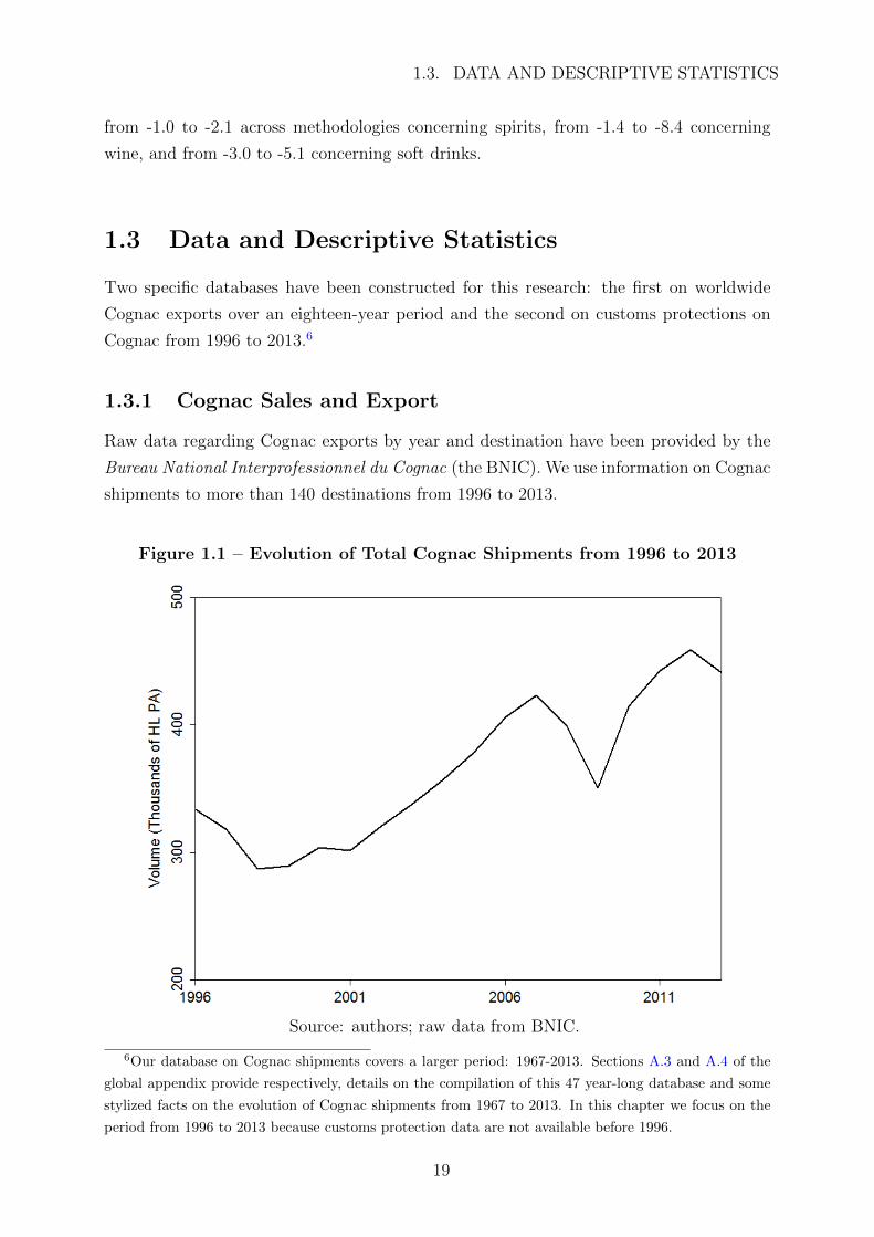
Figure 1.1 – Evolution of Total Cognac Shipments from 1996 to 2013
Source: authors; raw data from BNIC.
6Our database on Cognac shipments covers a larger period: 1967-2013. Sections A.3 and A.4 of the
global appendix provide respectively, details on the compilation of this 47 year-long database and some
stylized facts on the evolution of Cognac shipments from 1967 to 2013. In this chapter we focus on the
period from 1996 to 2013 because customs protection data are not available before 1996.
19

1.3. DATA AND DESCRIPTIVE STATISTICS
Figure 1.1 presents the evolution of total shipments, in volume, of Cognac from 1996 to
2013. Over these eighteen years, the volume of foreign shipments increased by 32 percent.
As shown by Figure 1.1, Cognac exports increase steadily during the first half of the 2000s
until the financial crisis in 2007-2008. Global sales recover by 2010.
Figure 1.2 – Evolution of the Export Unit Value of Cognac from 1996 to 2013
Source: authors; raw data from BNIC.
In 1996, the export unit value of Cognac is 4,402 euros/HL PA. Despite the ups and
downs, it increases by 21 percent between 1996 and 2013, reaching more than 5,313 eu-
ros/HL PA in 2013 (Figure 1.2). The average export unit value of Cognac during this
period is more than 4,133 euros/HL PA.
In 1996, Cognac was shipped to 160 countries. As shown in Figure 1.3, the number of
importing countries decreases to 150 in 2013. The concentration of destination markets
over time could be attributed to political factors, as some countries, particularly in Africa
have experienced episodes of internal armed conflicts during the period we are examining
(e.g., Chad, Libya, Syria and Uganda). These countries consecutively interrupted their
imports of Cognac. Other countries that ceased to import Cognac are small and by nature
volatile in terms of imports (e.g., Guyana, Northern Mariana Islands, Vanuatu, Wallis and
Futuna).
20

1.3. DATA AND DESCRIPTIVE STATISTICS
Figure 1.3 – Number of Destinations of Cognac Exports from 1996 to 2013
Source: authors; raw data from BNIC.
Figure 1.4 – Cognac Exports by Continent from 1996 to 2013
Source: authors; raw data from BNIC.
21

1.3. DATA AND DESCRIPTIVE STATISTICS
Figure 1.5 – Evolution of Cognac Exports to the Americas from 1996 to 2013
Source: authors; raw data from BNIC.
Figure 1.6 – Evolution of Cognac Exports to Asia* (Singapore and Hong Kong
excluded) from 1996 to 2013
Source: authors; raw data from BNIC.
22

1.3. DATA AND DESCRIPTIVE STATISTICS
Europe has long been the center of Cognac consumption. In the eighteenth century, the
first exports of Cognac were sent to England and northern Europe. Nevertheless, as shown
in Figure 1.4, since the beginning of the twenty-first century, the American and then the
Asian markets have become the most dynamic destinations for Cognac sales.
Figure 1.5 shows the evolution of Cognac exports to the Americas between 1996 and 2013.
The United States has always been by far the main destination on this continent; Cognac
exports to Canada and Latin America have been quite marginal.
In 2010, Asia became the top Cognac-importing continent. It is worth noting that Cognac
exports to Japan have continuously declined since the second half of the 1990s (see Figure
1.6). Exports to China, meanwhile, have substantially increased, making this destination
a current priority for Cognac houses. Meanwhile, Africa and Oceania are only marginal
destinations for Cognac exports, with less than 10,000 HL PA (around 3.6 million bottles)
each.
1.3.2 The Protection Database
Two types of customs instruments restrict worldwide exports of Cognac: ad valorem du-
ties (duties defined in percentage) and specific duties (defined in monetary units by units
of volume). In the study, we do not take into account domestic fiscality and in particular
consumption taxes levied on Cognac sales.7
Information on ad valorem and specific customs duties comes from the International Trade
Centre. While ad valorem duties were easy to treat, the only difficulty being the iden-
tification of the trade regime, most-favored-nation (MFN) or regional, we met several
difficulties in the treatment of specific duties. First, we converted all monetary amounts
to euros using annual averages of daily exchange rates observations from fxtop.com.8 Sec-
ond, the units of volume used in defining specific duties were harmonized to hectoliters
of pure alcohol. Specific duties were either defined by hectoliter, by hectoliter of pure
alcohol, by liter, or by liter of pure alcohol. We also met gallons under several definitions,
in particular either US gallons or imperial gallons.9 Specific duties are sometimes applied
7Available data at our disposal on excise duties cover only Organisation for Economic Co-operation
and Development (OECD) countries and a period of five years. Due to the small number of observations,
we do not include these data in any estimation.8Whenever fxtop.com data are missing, we resort to annual averages of midpoint daily rates from
oanda.com9The imperial gallon is defined as 4.54609 liters, and it is used in the United Kingdom, Canada, and
some Caribbean nations; the US gallon is defined as 3.785 liters and it is used in the US and some Latin
American and Caribbean countries.
23

1.3. DATA AND DESCRIPTIVE STATISTICS
on “per proof” gallons or liters.10
Table 1.111 indicates the summary statistics from this database, covering eighteen years
and more than a hundred importing countries. It shows that customs protections on
Cognac exports are very high. The simple average of ad valorem duties on all destina-
tion*year pairs is 42.8 percent when 0 are included, but 76.2 percent when 0 are excluded.
The highest ad valorem duty is 3,000 percent, which is still assessed in Egypt as of 2015.
Table 1.1 – Worldwide Customs Protection on Cognac: Statistics for more
than 100 Importing Countries, 1996-2013
AV Duty AVE of Spec. Duty Global AVE I
Min 0.0 % 0.0 % 0.00%
Max 3,000 % 129.6% 3,000 %
Simple Average 42.8 % 3.3 % 46.1 %
Median 10 % 0 % 17.1 %
Simple Average (0 excl.) 76.2% 21% 64.7%
AV = Ad Valorem; AVE = Ad Valorem Equivalent; excl. = excluding.
Source: authors; raw data from ITC.
Note that Table 1.1 shows the average world protection on line HS6 220820: Spirits ob-
tained by distilling grape wines or grape marcs (grape brandy).12 Therefore this line
mainly concerns Cognac. The world average customs duty on this line does not differ
much from the one on other alcoholic beverages, except for beer, which is taxed at sig-
nificantly lower rates (see Graph 1.7 in the appendix to chapter one).13 Protection is
already high on mineral waters, sodas, fruit and vegetable juice (lines 220110 to 220290),
lower on vinegar (220900), and very high on alcoholic beverages (220300 to 220890). Con-
sequently, protection on brandies is comparable to protection on other alcoholic beverages.
The simple average of specific duties in ad valorem equivalent, is 3.3 percent. To estimate
10A proof gallon is one liquid gallon of spirits that is 50 percent alcohol at 60 degrees Fahrenheit. So
distilled spirits bottled at 80 proof (40 percent alcohol) are 0.8 proof gallons per gallon of liquid.11The statistics displayed in Table 1.1 are calculated for the period from 1996 to 2013 and for countries
that have registered positive Cognac trade flows.12HS stands for Harmonized Commodity Description and Coding Systems, an international nomencla-
ture for the classification of products. All countries use the same classification up to the six-digit level,
the most specific one, of the HS (Source: United Nations Trade Statistics).13Data on the world average customs duties (in ad valorem equivalent) for chapter 22 - Beverages,
spirits and vinegar - of the HS6 nomenclature come from the MAcMap Database.
24

1.4. ECONOMETRIC ESTIMATION
ad valorem equivalents of specific duties (column 3) we divide the specific duty by the
yearly average unit value. We take the annual average unit value and not the bilateral
unit value to avoid an endogeneity bias; high specific duties could lead to a change in
the composition of the quality exported to decrease protection in relative terms. The
last column of Table 1.1 indicates a global average by adding the different elements of
customs protections. National customs protections on Cognac vary from 0 percent to
3,000 percent.
1.4 Econometric Estimation
In this section, we first detail our empirical strategy. Then, we present and discuss our
results and conduct robustness checks.
1.4.1 Empirical Strategy and Data
Our evaluation of the determinants of Cognac exports is based on a gravity equation.14
In this model, exports depend on demand (usually proxied by the GDP of importing
country), supply (GDP of exporting country) and trade costs (tariffs and transportation
costs proxied by distance and other geographical and historical factors).
Our equation presents specific features. First, as we perform estimations only on French
exports, we do not need the exporter’s GDP; supply can be controlled using time-fixed
effects.
Second, we add importer’s per-capita GDP and religious factors to take into considera-
tion the characteristics of Cognac demand, as a luxury product and an alcoholic beverage.
Third, Anderson and van Wincoop (2003) recommend using relative trading costs in the
gravity equation rather than absolute trading costs. In our specification, we do not need
to construct a relative distance indicator and relative protection rate since all exports are
from France.
Fourth, following Helpman, Melitz, and Rubinstein (2008), we consider the case where
the sample of destinations of Cognac exports is nonrandom. In such a case conventional
estimators, such as ordinary least squares (OLS), applied on a sample of nonzero exports
would be biased; thus, it is best to adopt Heckman’s (1979) procedure to correct the sam-
ple selection issue. In our case, a right selection variable is the armed conflict variable, a
dummy equal to one if importing countries have experienced internal armed conflicts in
14See Head and Mayer (2014) for a complete presentation.
25

1.4. ECONOMETRIC ESTIMATION
a given year. We explain in section 1.3.1 that many countries that have ceased importing
Cognac have experienced episodes of internal armed conflict.
Let Qjt be the volume of Cognac exported to country j at year t. We estimate the fol-
lowing equation, using Heckman’s (1979) procedure:
ln(Qjt) = α0 + α1ln(Yjt) + α2ln(yjt) + α3ln(dj) + α4ln(ejt)
+ α5ln(AV Ejt) + α6Llj + α7Relj + α8Conflictjt + νt + ujt (1.1)
where Yjt is country j’s GDP at year t, yjt is the per-capita GDP of country j at year t,
dj is the distance from France to country j, ejt is the nominal exchange rate of country j’s
currency against the euro, AV Ejt is the global average customs protection on brandy15
(ad valorem equivalent), implemented by country j at year t (see section 1.3.2).
Other variables are dummies: Llj is a dummy taking the value 1 if country j is landlocked,
Relj is a dummy taking the value 1 if fifty percent or more of country j’s population is
Muslim, Conflictjt is a dummy taking the value 1 if country j has been involved in an in-
ternal armed conflict or internationalized internal armed conflict16 in year t that resulted
in at least one thousand battle-related deaths in that given year. Finally, νt are time fixed
effects and ujt is the error term.17
Data on each country j’s GDP and per-capita GDP are in constant 2005 U.S. dollars and
were retrieved from the World Bank’s World Development Indicators DataBank. Nom-
inal exchange rates are annual averages of daily observations from fxtop.com,18 and we
use Centre d’Etudes Prospectives et d’Informations Internationales’ (CEPII’s) weighted
bilateral distance measure (in kilometers). The variables Llj and Relj are from CEPII
15HS6 220820: Spirits obtained by distilling grape wine or grape marc.16The definition of armed conflict used here is given by the Uppsala Conflict Data Program (UCDP):
“An armed conflict is a contested incompatibility that concerns government and/or territory where the
use of armed force between two parties, of which at least one is the government of a state, results in at
least 25 battle-related deaths in one calendar year.” For more information on the definition and type of
conflict see the UCDP/PRIO Armed Conflict Dataset Codebook1, version 4-2015; Gleditsch et al. (2002)
and Pettersson and Wallensteen (2015).17We use a gravity equation based on a standard approach in which products are considered to be
normal goods, and we implicitly assume that income distribution within a country plays no role in the
aggregate demand. To control for this assumption, we include the Gini index of the importing country.
Data are retrieved from UNU-WIDER’s, World Income Inequality Database (WIID3c), September 2015.
However, including this variable considerably reduces the size of the sample and yields biased estimation
results. These results and further details on the sample bias are provided in the appendix to chapter one,
section 1.A.18Whenever fxtop.com data were missing, we resorted to annual averages of midpoint daily rates from
oanda.com
26

1.4. ECONOMETRIC ESTIMATION
and the CIA Factbook respectively.19 Data on armed conflicts are retrieved from the
UCDP/PRIO Armed Conflict Dataset v.4-2015.
Summary statistics of the aforementioned variables and the list of all importing countries
in 2013 are provided in the appendix to chapter 1, Tables 1.10 and 1.11 respectively.
Equation 1.1 was estimated for the period 1996− 2013.
1.4.2 Results
The top and bottom of Table 1.2 report the results of the estimation of equation 1.1, using
Heckman’s (1979) procedure. The Wald test on the independence of equations suggests
the presence of a selection bias.
In column 1 we use the full panel of importing countries. As the international Cognac
trade is characterized by a high level of re-exportation from a limited number of countries
(Hong Kong, the Netherlands, Panama, Singapore and United Arab Emirates; list pro-
vided by the BNIC), in column 2 of Table 1.2, we conduct a robustness test by excluding
these destinations. The re-exporting status of these destinations has been confirmed by
an analysis of their alcohol consumption.20
“Traditional” gravity variables have significant coefficients with the expected sign: the im-
porting country’s GDP has a significant and positive impact on Cognac exports, whether
on the probability of trade (the extensive margin) or the trade volume (the intensive
margin). Distance, on the other hand, has the opposite effect, both on the probability of
trade and on the trade volume.
The per-capita GDP of the destination country has a positive impact both on the exten-
sive and intensive margins of trade. Being landlocked acts as a trade barrier, restricting
both the positive trade volume and the probability of trade. The dummy variable control-
ling for religious factors in the destination markets has a negative impact on the extensive
and intensive margins.
19The list of Muslim-majority countries with the corresponding date of information according to the
CIA Factbook is provided in the appendix to chapter 1, Table 1.12.20Within the limits of data availability, we compared the average Cognac exports to these destinations
from 1996 to 2013 with their average per-capita adult (fifteen years or older) consumption of alcohol.
These data come from the World Health Organization. For the Netherlands, Panama, and United Arab
Emirates we estimate that the per-capita Cognac consumption (exports) represents on average 0.6, 0.4
and 0.7 percent of the total per-capita alcohol consumption in these countries respectively. These figures
are above our estimated world average (0.13). In the case of Singapore, it is as high as 56 percent. Note
that data on adult per-capita alcohol consumption for Hong Kong were not available so no comparisons
were made.
27

1.4. ECONOMETRIC ESTIMATION
The exchange rate has a significant positive impact on the probability of trade and the
opposite effect on the intensive margin, which means that an appreciation of the euro in-
creases the probability of trade but decreases Cognac trade volumes. The decision in favor
of exporting Cognac to a given destination depends on whether local sales are enough to
cover for fixed costs of establishing a positive trade flow. When the euro appreciates,
the price of the local currency (destination’s currency) against the euro decreases, which
implies that fixed trade costs in local currency also decrease. Therefore, as long as these
costs are in the local currency, it is not surprising that the impact of the exchange rate
on the extensive margin is positive.21 This positive effect of the exchange rate on the
extensive margin of trade, as well as the negative effect on the intensive margin, have
some theoretical foundations (see for example Chaney, 2013).22
Customs protections have no impact on the intensive margin but they have a positive
and significant one on the extensive margin. These results are robust to the exclusion of
re-exporting countries.
The significant positive impact of customs duties on the extensive margin of trade means
that an increase of a tariff on Cognac leads to an increase in the probability of exporting
the product. We suspect the presence of an endogeneity bias, so that the tariff may be
induced by Cognac imports. Many importing countries are small and/or developing coun-
tries with a limited domestic fiscal base. Because Cognac imports are often associated
with conspicuous consumption, governments may react to imports of this product on its
territory by imposing customs duties. Customs duties are a politically appreciated source
of public revenue (there is a large literature on endogenous protectionism)23. This effect
is exacerbated considering that Cognac brandy is a vice product and might be the object
of high taxation, not only excise duties but also customs duties. Increases in Cognac
imports may encourage local authorities to augment customs duties on this product, in
order to collect more revenues and fight the consumption of a vice product.
To correct for this potential bias, we use an instrumental variables (IV) approach for
probit models. We use tax revenues in percentage of GDP as an instrument for the global
ad valorem equivalent.24 As explained in the previous paragraph, customs duties are a
21When we correct for the endogeneity bias we find a nonsignificant impact of the exchange rate on
the probability of trade; see Table 1.3.22“Since the entry cost into the foreign market is paid in foreign currency, this means a relaxation of
the liquidity constraint for constrained exporters” (Chaney, 2013, p. 22).23See for example Mayer (1984), Baldwin (1985), Trefler (1993).24Annual data on tax revenues as percentage of GDP of the budgetary central governments of des-
tination countries are collected from the International Monetary Fund’s (IMF’s) Government Finance
28
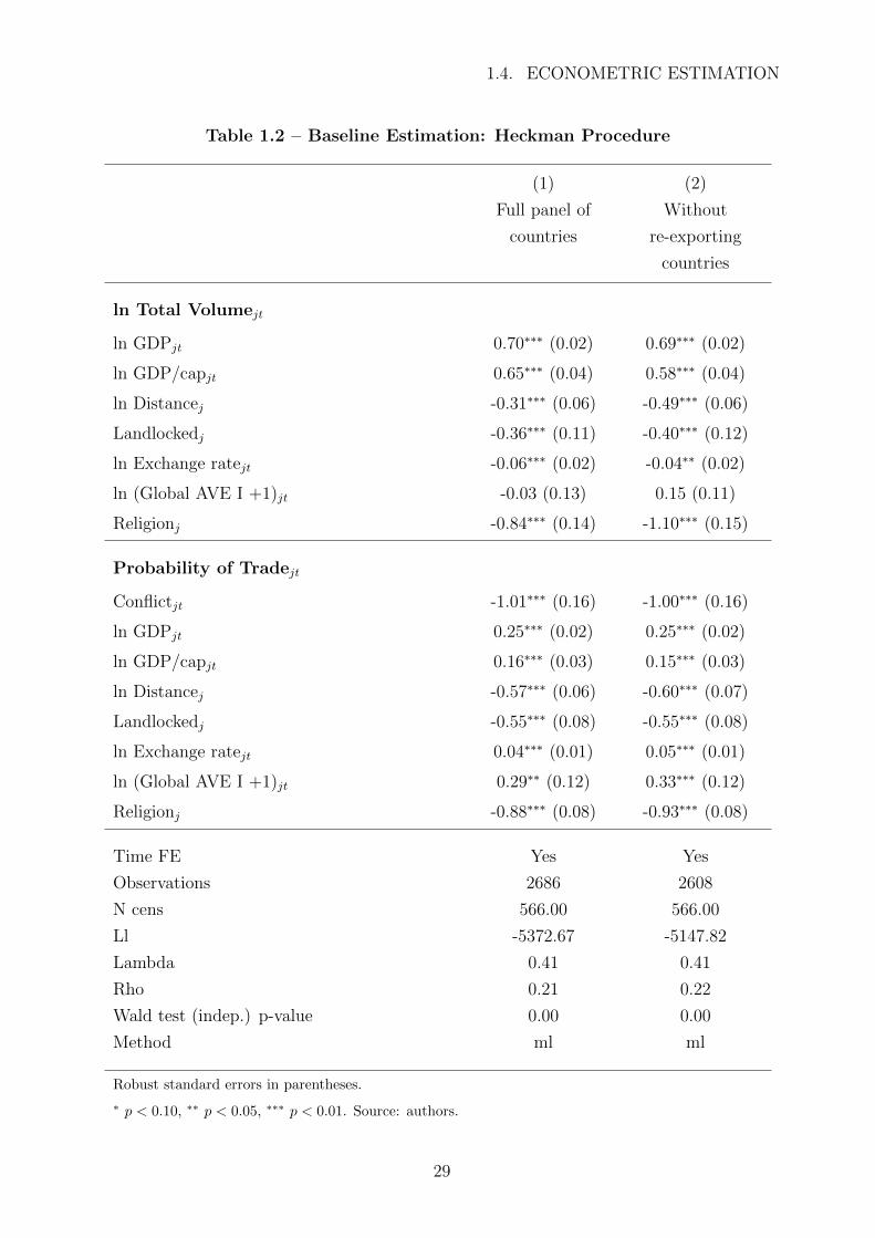
1.4. ECONOMETRIC ESTIMATION
Table 1.2 – Baseline Estimation: Heckman Procedure
(1) (2)
Full panel of
countries
Without
re-exporting
countries
ln Total Volumejt
ln GDPjt 0.70∗∗∗ (0.02) 0.69∗∗∗ (0.02)
ln GDP/capjt 0.65∗∗∗ (0.04) 0.58∗∗∗ (0.04)
ln Distancej -0.31∗∗∗ (0.06) -0.49∗∗∗ (0.06)
Landlockedj -0.36∗∗∗ (0.11) -0.40∗∗∗ (0.12)
ln Exchange ratejt -0.06∗∗∗ (0.02) -0.04∗∗ (0.02)
ln (Global AVE I +1)jt -0.03 (0.13) 0.15 (0.11)
Religionj -0.84∗∗∗ (0.14) -1.10∗∗∗ (0.15)
Probability of Tradejt
Conflictjt -1.01∗∗∗ (0.16) -1.00∗∗∗ (0.16)
ln GDPjt 0.25∗∗∗ (0.02) 0.25∗∗∗ (0.02)
ln GDP/capjt 0.16∗∗∗ (0.03) 0.15∗∗∗ (0.03)
ln Distancej -0.57∗∗∗ (0.06) -0.60∗∗∗ (0.07)
Landlockedj -0.55∗∗∗ (0.08) -0.55∗∗∗ (0.08)
ln Exchange ratejt 0.04∗∗∗ (0.01) 0.05∗∗∗ (0.01)
ln (Global AVE I +1)jt 0.29∗∗ (0.12) 0.33∗∗∗ (0.12)
Religionj -0.88∗∗∗ (0.08) -0.93∗∗∗ (0.08)
Time FE Yes Yes
Observations 2686 2608
N cens 566.00 566.00
Ll -5372.67 -5147.82
Lambda 0.41 0.41
Rho 0.21 0.22
Wald test (indep.) p-value 0.00 0.00
Method ml ml
Robust standard errors in parentheses.
∗ p < 0.10, ∗∗ p < 0.05, ∗∗∗ p < 0.01. Source: authors.
29

1.4. ECONOMETRIC ESTIMATION
Table 1.3 – Baseline Estimation: IV Probit
(1) (2)
Full panel of
countries
Without
re-exporting
countries
Probability of Tradejt
ln (Global AVE I +1)jt -1.99∗∗∗ (0.49) -1.96∗∗∗ (0.49)
ln GDPjt 0.13∗∗∗ (0.04) 0.13∗∗∗ (0.04)
ln GDP/capjt -0.07 (0.09) -0.07 (0.08)
ln Distancej -0.27 (0.17) -0.27 (0.18)
Landlockedj -0.79∗∗∗ (0.14) -0.79∗∗∗ (0.14)
ln Exchange ratejt -0.04 (0.02) -0.04 (0.02)
Religionj 0.36 (0.26) 0.36 (0.25)
Conflictjt -0.46∗∗ (0.19) -0.46∗∗ (0.19)
Time FE Yes Yes
Observations 1261 1244
Ll -985.05 -982.11
Wald test (exog.) p-value 0.03 0.03
Instrument ln Tax Revenue ln Tax Revenue
Method ml ml
Robust standard errors in parentheses.
∗ p < 0.10, ∗∗ p < 0.05, ∗∗∗ p < 0.01. Source: authors.
source of public revenue and therefore correlated with our instrument. On the other hand,
we have no reason to believe that the volume of Cognac exports is correlated with tax
revenues.25
Results of the IV estimation on the probability of trade are presented in Table 1.3. The
hypothesis of exogeneity of the instrumented variable is rejected. Correcting for the
Statistics.25We also conducted a Heckman test with lagged (one-year) customs duties in place of current customs
duties; see Table 1.15 in the appendix to chapter one. We obtain the same results as those shown in
Table 1.2. Since import duties are quite stable over time this is not surprising.
30

1.4. ECONOMETRIC ESTIMATION
endogeneity bias shows that customs duties have a significant negative impact on the ex-
tensive margin, which is in line with the literature. The GDP of destination countries has
a significant positive impact. The per-capita GDP, distance, exchange rate and religion
variables no longer have a significant impact, while being landlocked and experiencing
armed conflicts negatively influence the probability of trade. These results are robust to
the exclusion of re-exporting countries.
1.4.3 Discussion
We compare the results of Table 1.2 with those in the existing literature, particularly with
studies focusing on the determinants of high-end versus low-end export flows.
According to our estimations, the elasticity of Cognac exports to the GDP of the im-
porting country is 0.7 (0.69 when excluding re-exporting countries; see column 2). This
estimated coefficient is greater than that for all luxury products considered all together,
according to Fontagne and Hatte (2013): 0.461 when considering worldwide export flows
and 0.556 in the case of French export flows. The destination country’s per-capita GDP
impact on Cognac trade flows, estimated at an order of magnitude of 0.65 (0.58 when ex-
cluding re-exporting countries), is also greater compared to Fontagne and Hatte’s (2013)
estimations (0.3145 and 0.394 in the case of worldwide and French high-end export flows,
respectively) but is lower than Martin and Mayneris’ (2015) results, (0.87) which are based
on aggregated French firm-level data for two-hundred products in 2005. The impact of
distance on Cognac exports is lower in absolute value compared to all luxury products in
Fontagne and Hatte (2013): -0.31 in the case of Cognac; -0.734 and -0.578 for worldwide
and French exports, respectively. Thus, Cognac is a luxury product whose exports are
negatively affected by distance, but it is much less sensitive to distance than other prod-
ucts, including other luxury products.26 At the same time, customs protections have no
significant impact on the intensive margin of trade.
We do not find this result surprising given the nature of our product. Using the same
argument, one may expect a nonsignificant impact of the distance variable. However, even
though distance is a relatively good proxy of transportation costs (in which case, for all
else equal, a nonsignificant impact is indeed a plausible hypothesis), it includes influences
of other factors like information costs.27
26Fontagne and Hatte (2013) base their estimations on OLS with distance, GDP, and per-capita GDP
as covariates. Martin and Mayneris’ (2015) baseline estimation uses per-capita GDP, population and
distance as covariates in an OLS regression. Note that our estimation methodology differs from that of
these authors in that we evaluate the impact of the determinants of Cognac trade flows by correcting for
a selection bias using Heckman’s (1979) procedure.27Another explanation for the nonsignificant impact of customs duties on Cognac trade flows is that
31

1.4. ECONOMETRIC ESTIMATION
1.4.4 Robustness tests
We perform three tests in order to check the robustness of our results. First, we estimate
equation 1.1 using an alternative measure of customs protections. Second, we estimate
equation 1.1 adding continents fixed effects. Third, we use the Poisson Pseudo Maximum
Likelihood and the EK Tobit models (PPML and EK Tobit respectively) as alternative
estimation methods.28
We use a different computation of the average protection on Cognac to test the robust-
ness of our baseline results (see Table 1.4). The ad valorem equivalent of specific duties is
either calculated by dividing the specific duty expressed in euros by HL PA by the annual
average unit value on flows to all destinations (the methodology used in Table 1.1 and in
central estimations) or by the unit value of the flow to a specific destination (ln Global
AVE II ). This alternative measure of customs protections leads to the same results-that
is, customs duties have no impact on the intensive margin, but a significant and pos-
itive impact on the extensive margin. When correcting for the endogeneity bias using
the IV estimation method (see Table 1.5), we find that customs protections have a sig-
nificant but negative impact. Results concerning the rest of the variables remain the same.
In Table 1.6, we estimate equation 1.1 adding continents’ fixed effects. We add five dum-
mies for: Africa, Americas, Asia, Europe and Oceania.29 We exclude distance and religion
variables because of possible intracontinent correlation. We find qualitatively similar re-
sults to our baseline estimation results when conducting the Heckman procedure (see
Table 1.6) and correcting for the endogeneity bias (Table 1.7), regardless of whether we
exclude re-exporting countries.
As additional robustness checks, we use a PPML approach to estimate the determinants
of Cognac trade flows. The estimation considers “0” trade flows (see Table 1.8). In
Table 1.9 we show the results of a Tobit estimation based on Eaton and Kortum’s (2001)
method (EK Tobit). We find qualitatively similar results to the previous ones using both
approaches.
many importing countries also rely on excise duties on Cognac as a source of public revenue. This theory
was confirmed during discussions with the BNIC. However, as stated previously, we cannot check their
impact econometrically.28In the appendix to chapter one, section 1.B we also provide some evidence on the determinants of
Cognac export unit values.29The list of countries by continents is shown in the appendix to chapter one, Table 1.16. The assign-
ment of countries to continents is based on the United Nations Statistics Division’s list of geographic
regions.
32

1.4. ECONOMETRIC ESTIMATION
Table 1.4 – Robustness Check I: Alternative Customs Protection Measure:
Heckman Procedure
(1) (2)
Full panel of
countries
Without
re-exporting
countries
ln Total Volumejt
ln GDPjt 0.70∗∗∗ (0.02) 0.69∗∗∗ (0.02)
ln GDP/capjt 0.65∗∗∗ (0.04) 0.58∗∗∗ (0.04)
ln Distancej -0.31∗∗∗ (0.06) -0.49∗∗∗ (0.06)
Landlockedj -0.36∗∗∗ (0.11) -0.40∗∗∗ (0.12)
ln Exchange ratejt -0.06∗∗∗ (0.02) -0.04∗∗ (0.02)
ln (Global AVE II +1)jt -0.03 (0.13) 0.15 (0.11)
Religionj -0.84∗∗∗ (0.14) -1.10∗∗∗ (0.15)
Probability of Tradejt
Conflictjt -1.01∗∗∗ (0.16) -1.00∗∗∗ (0.16)
ln GDPjt 0.25∗∗∗ (0.02) 0.25∗∗∗ (0.02)
ln GDP/capjt 0.16∗∗∗ (0.03) 0.15∗∗∗ (0.03)
ln Distancej -0.57∗∗∗ (0.06) -0.60∗∗∗ (0.07)
Landlockedj -0.55∗∗∗ (0.08) -0.55∗∗∗ (0.08)
ln Exchange ratejt 0.04∗∗∗ (0.01) 0.05∗∗∗ (0.01)
ln (Global AVE II +1)jt 0.29∗∗ (0.12) 0.33∗∗∗ (0.12)
Religionj -0.88∗∗∗ (0.08) -0.93∗∗∗ (0.08)
Time FE Yes Yes
Observations 2686 2608
N cens 566.00 566.00
Ll -5372.67 -5147.82
Lambda 0.41 0.41
Rho 0.21 0.22
Wald test (indep.) p-value 0.00 0.00
Method ml ml
Robust standard errors in parentheses.
∗ p < 0.10, ∗∗ p < 0.05, ∗∗∗ p < 0.01. Source: authors.
33

1.4. ECONOMETRIC ESTIMATION
Table 1.5 – Robustness Check I: Alternative Customs Protection Measure: IV
Probit
(1) (2)
Full panel of
countries
Without
re-exporting
countries
Probability of Tradejt
ln (Global AVE II +1)jt -1.99∗∗∗ (0.49) -1.96∗∗∗ (0.49)
ln GDPjt 0.13∗∗∗ (0.04) 0.13∗∗∗ (0.04)
ln GDP/capjt -0.07 (0.09) -0.07 (0.08)
ln Distancej -0.27 (0.17) -0.27 (0.18)
Landlockedj -0.79∗∗∗ (0.14) -0.79∗∗∗ (0.14)
ln Exchange ratejt -0.04 (0.02) -0.04 (0.02)
Religionj 0.36 (0.26) 0.36 (0.25)
Conflictjt -0.46∗∗ (0.19) -0.46∗∗ (0.19)
Time FE Yes Yes
Observations 1261 1244
Ll -985.05 -982.11
Wald test (exog.) p-value 0.03 0.03
Instrument ln Tax Revenue ln Tax Revenue
Method ml ml
Robust standard errors in parentheses.
∗ p < 0.10, ∗∗ p < 0.05, ∗∗∗ p < 0.01. Source: authors.
34
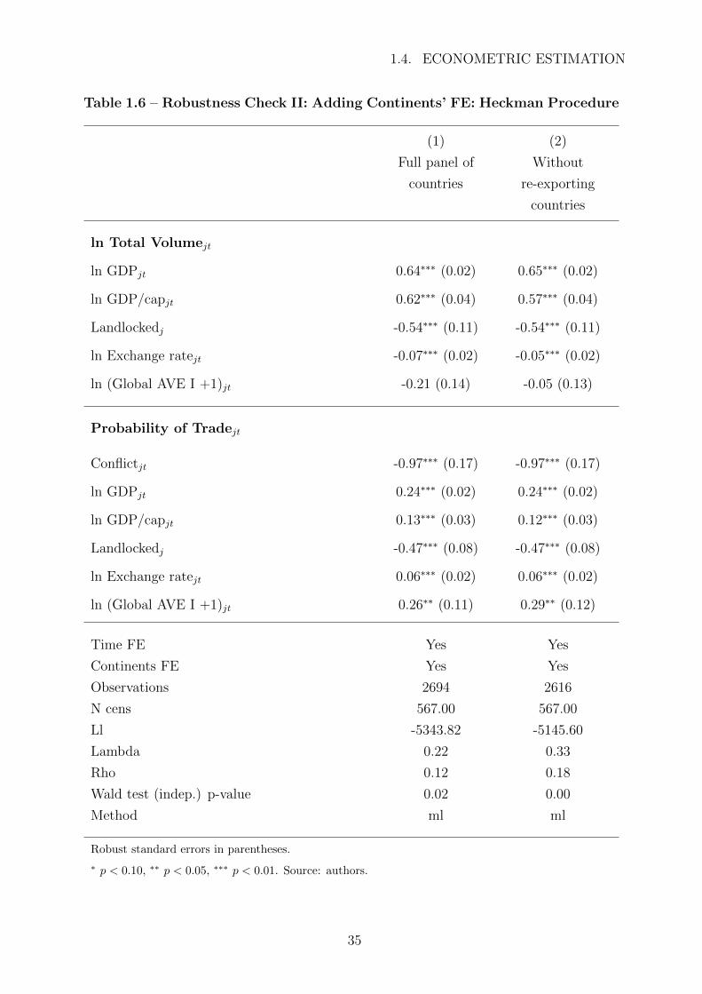
1.4. ECONOMETRIC ESTIMATION
Table 1.6 – Robustness Check II: Adding Continents’ FE: Heckman Procedure
(1) (2)
Full panel of
countries
Without
re-exporting
countries
ln Total Volumejt
ln GDPjt 0.64∗∗∗ (0.02) 0.65∗∗∗ (0.02)
ln GDP/capjt 0.62∗∗∗ (0.04) 0.57∗∗∗ (0.04)
Landlockedj -0.54∗∗∗ (0.11) -0.54∗∗∗ (0.11)
ln Exchange ratejt -0.07∗∗∗ (0.02) -0.05∗∗∗ (0.02)
ln (Global AVE I +1)jt -0.21 (0.14) -0.05 (0.13)
Probability of Tradejt
Conflictjt -0.97∗∗∗ (0.17) -0.97∗∗∗ (0.17)
ln GDPjt 0.24∗∗∗ (0.02) 0.24∗∗∗ (0.02)
ln GDP/capjt 0.13∗∗∗ (0.03) 0.12∗∗∗ (0.03)
Landlockedj -0.47∗∗∗ (0.08) -0.47∗∗∗ (0.08)
ln Exchange ratejt 0.06∗∗∗ (0.02) 0.06∗∗∗ (0.02)
ln (Global AVE I +1)jt 0.26∗∗ (0.11) 0.29∗∗ (0.12)
Time FE Yes Yes
Continents FE Yes Yes
Observations 2694 2616
N cens 567.00 567.00
Ll -5343.82 -5145.60
Lambda 0.22 0.33
Rho 0.12 0.18
Wald test (indep.) p-value 0.02 0.00
Method ml ml
Robust standard errors in parentheses.
∗ p < 0.10, ∗∗ p < 0.05, ∗∗∗ p < 0.01. Source: authors.
35

1.4. ECONOMETRIC ESTIMATION
Table 1.7 – Robustness Check II: Adding Continents’ FE: IV Probit
(1) (2)
Full panel of
countries
Without
re-exporting
countries
Probability of Tradejt
ln (Global AVE I +1)jt -1.86∗∗∗ (0.52) -1.83∗∗∗ (0.53)
ln GDPjt 0.14∗∗∗ (0.04) 0.14∗∗∗ (0.04)
ln GDP/capjt -0.08 (0.08) -0.07 (0.07)
Landlockedj -0.80∗∗∗ (0.15) -0.79∗∗∗ (0.15)
ln Exchange ratejt -0.03 (0.02) -0.04 (0.03)
Conflictjt -0.44∗∗ (0.18) -0.45∗∗ (0.18)
Time FE Yes Yes
Continents FE Yes Yes
Observations 1261 1244
Ll -1019.95 -1012.81
Wald test (exog.) p-value 0.04 0.04
Instrument ln Tax Revenue ln Tax Revenue
Method ml ml
Robust standard errors in parentheses.
∗ p < 0.10, ∗∗ p < 0.05, ∗∗∗ p < 0.01. Source: authors.
36

1.4. ECONOMETRIC ESTIMATION
Table 1.8 – Robustness Check IIIa: Alternative Estimation Method: PPML
(1)
Full panel of countries
ln GDPjt 0.95∗∗∗ (0.04)
ln GDP/capjt 0.14 (0.10)
ln Distancej 0.02 (0.03)
Landlockedj -0.59∗∗∗ (0.11)
ln Exchange ratejt -0.15∗∗∗ (0.02)
ln (Global AVE I +1)jt -0.67∗∗ (0.33)
Religionj -0.23 (0.19)
Time FE Yes
Observations 2686
Robust standard errors in parentheses.
∗ p < 0.10, ∗∗ p < 0.05, ∗∗∗ p < 0.01. Source: authors.
37

1.5. CONCLUSION
Table 1.9 – Robustness Check IIIb: Alternative Estimation Method: EK Tobit
(1)
Full panel of countries
ln GDPjt 0.78∗∗∗ (0.03)
ln GDP/capjt 0.77∗∗∗ (0.05)
ln Distancej -0.47∗∗∗ (0.07)
Landlockedj -0.63∗∗∗ (0.17)
ln Exchange ratejt -0.05∗∗ (0.03)
ln (Global AVE I +1)jt 0.15 (0.17)
Religionj -1.69∗∗∗ (0.20)
Time FE Yes
Observations 2503
N uncensored 2120.00
N left-censored 383.00
N right-censored 0.00
Ll -5510.49
Robust standard errors in parentheses.
∗ p < 0.10, ∗∗ p < 0.05, ∗∗∗ p < 0.01. Source: authors.
1.5 Conclusion
In this chapter, we present a new database on Cognac exports to more than one hundred
countries spanning a period of eighteen years. We successively evaluate the extensive and
the intensive margins of trade, and we confirm a result from the literature positing that
the sale of luxury products is less sensitive to distance; in the case of Cognac, sales are
even less sensitive than other luxury products.
On the other hand, customs duties have no significant impact on the intensive margin but
a positive one on the probability of trade. While the former result is not surprising given
the nature of Cognac, but the latter is counterintuitive. We suspect the presence of an
endogeneity bias, because tariffs represent in many countries a significant source of public
revenue. Correcting for this bias leads to a significant and negative impact of customs
protection on the extensive margin. The other covariates have the expected impact on
38

1.5. CONCLUSION
Cognac exports.
In the introduction to this chapter, we question the reasons behind Cognac’s global suc-
cess. The first determinant of the number of Cognac exports is economic growth world-
wide. The second reason is that exports of Cognac are not very (relatively) affected by
transportation costs.
Future work is still needed to fully understand the Cognac sector. In particular, the
database of Cognac exports offers a precise measurement of quality, by the age of the
youngest eau-de-vie incorporated in the brandy. This is a better measurement of quality
than the unit value or price, which are often used in the literature, or than a subjective
expert’s ranking. The structure by quality of exports is the object of chapter two.
39


Appendix to Chapter 1
Figure 1.7 – World Average Customs Duties: Chapter 22 at the HS6 Level
Source: authors; data from MAcMap.
41

Table 1.10 – Summary Statistics
Variable Obs. Mean Std.
Dev.
Min. Max.
Total Volume (HL PA) 4,230 1,551.865 9,442.746 0 156,656.086
GDP (constant 2005 USD) 3,357 2.33e+11 1.05e+11 1.75e+07 1.45e+13
GDP/cap (constant 2005 USD) 3,357 10,559.387 17,203.069 73 158,603
Distance (km) 3,888 6,708.002 4,300.071 473.73 18,894.29
Exchange Rate (loc. curr. to 1 e) 4,117 2,408.157 49,052.639 0.002 1,777,042.822
AVE I 2,829 0.428 2.262 0 30
Landlocked 4,176 0 1
Religion 4,068 0 1
Conflict 4,230 0 1
Source: authors.
42

Table 1.11 – List of Cognac Importing Countries in 2013
Albania Gabon Nigeria
Algeria Georgia Norway
American Oceania Germany Oman
Andorra Ghana Panama
Angola Gibraltar Paraguay
Antigua and Barbuda Greece Peru
Argentina Grenada Philippines (the)
Armenia Guatemala Poland
Aruba Guinea Portugal
Australia Haiti Qatar
Austria Honduras Romania
Azerbaijan Hong Kong Russian Federation (the)
Bahamas (the) Hungary Saint Barthelemy
Bahrain Iceland Saint Kitts and Nevis
Barbados India Saint Lucia
Belarus Indonesia Saint Pierre and Miquelon
Belgium and Luxembourg Iraq Saint Vincent and the Grenadines
Benin Ireland Senegal
Bermuda Israel Serbia
Bosnia and Herzegovina Italy Seychelles
Brazil Jamaica Sierra Leone
Bulgaria Japan Singapore
Burkina Faso Jordan Slovakia
Cambodia Kazakhstan Slovenia
Cameroon Kenya South Africa
Canada Korea (the Republic of) Spain
Cayman Islands (the) Kyrgyzstan Sri Lanka
Chile Lao People’s Democratic Republic (the) Suriname
China Latvia Sweden
Colombia Lebanon Switzerland
Congo Lithuania Taiwan (Province of China)
Congo (the Democratic Republic of the) Macao Tajikistan
Costa Rica Macedonia (the former Yugoslav Republic of) Tanzania, United Republic of
Croatia Malaysia Thailand
Cuba Maldives Togo
Cyprus Mali Trinidad and Tobago
Czech Republic (the) Malta Tunisia
Cote d’Ivoire Mauritius Turkey
Denmark Mexico Turkmenistan
Djibouti Mongolia Turks and Caicos Islands (the)
Dominican Republic (the) Montenegro Ukraine
Ecuador Montserrat United Arab Emirates (the)
Egypt Morocco United Kingdom (the)
El Salvador Myanmar United States (the)
Equatorial Guinea Nepal Uruguay
Estonia Netherlands (the) Uzbekistan
Ethiopia Netherlands Antilles Venezuela, Bolivarian Republic of
Fiji New Caledonia Viet Nam
Finland New Zealand Virgin Islands (British)
French Polynesia Niger (the) Virgin Islands (U.S.)
Source: authors; raw data from BNIC.
43

Table 1.12 – List of Muslim-Majority Countries with their Dates of Informa-
tion according to the CIA Factbook
Afghanistan NA Malaysia 2010
Albania 2011 Maldives NA
Algeria 2012 Mali 2009
Azerbaijan 1995 Mauritania NA
Bahrain 2010 Morocco 2010
Bangladesh 2004 Niger (the) NA
Brunei Darussalam 2011 Nigeria NA
Burkina Faso 2006 Oman 2010
Chad 1993 Pakistan 2010
Cocos (Keeling) Islands (the) 2002 Panama NA
Comoros NA Qatar 2004
Djibouti NA Saudi Arabia 2013
Egypt 2012 Senegal NA
Eritrea NA Sierra Leone NA
French Polynesia NA Somalia NA
Gambia (The) NA Sudan (the) NA
Guinea NA Syrian Arab Republic (the) NA
Indonesia 2010 Tajikistan 2003
Iran (the Islamic Republic of) 2011 Tunisia NA
Iraq 2010 Turkey NA
Jordan 2010 Turkmenistan NA
Kazakhstan 2009 United Arab Emirates (the) 2005
Kuwait 2013 Uzbekistan NA
Kyrgyzstan NA Western Sahara* NA
Lebanon 2012 Yemen 2010
Libya 2010
NA = Not Available. Source: CIA Factbook.
44

1.A. INCOME DISPARITY AND THE GRAVITY EQUATION
1.A Income Disparity and the Gravity Equation
We control for income disparity in equation 1.1 adding the GINI index. However, this
variable is documented for only 56 countries (or less, depending on the period) and its
inclusion considerably reduces the size of the sample (from 2686 to 1099 observations).
Moreover, the information we have on the GINI index is not randomly distributed as
shown in Table 1.13, leading to a potential sample bias. Countries for which we have
information on the GINI index appear to have in average higher GDP, per-capita GDP,
exchange rates and apply lower tariffs on Cognac imports.
The estimation of our baseline specification on this reduced sample confirms the bias
(see Table 1.14; the Heckman estimator does not converge on the reduced sample). For
example, while the religion dummy has a negative impact on Cognac’s volumes of exports,
when we consider the entire database, it does not have any effect in the reduced sample.
On the other hand, the estimated coefficient of the tariff is positive and significant on
the reduced sample whereas it was not significant on the entire database. We therefore
conclude that including this variable yields biased estimation results.
Table 1.13 – Summary Statistics: Full Sample vs. Gini Sample
Variable Sample Obs. Mean Std.
Dev.
Min. Max.
GDPjtFull 3,357 2.33e+11 1.05e+11 1.75e+07 1.45e+13
Gini 1,264 4.62e+11 1.56e+12 2.38e+07 1.45e+13
GDP/capjtFull 3,357 10,559.387 17,203.069 73 158,603
Gini 1,264 12,677.293 16,072.835 133 69,095
DistancejFull 3,888 6,708.002 4,300.071 473.73 18,894.29
Gini 1,288 5,148.109 4,017.131 473.73 18,894.29
Exchange ratejtFull 4,117 2,408.157 49,052.639 0.002 1,777,042.822
Gini 1,271 3,834.084 64,437.231 0.036 1,694,851.106
Global AVE IjtFull 2,829 0.428 2.262 0 30
Gini 1,160 0.322 1.986 0 30
Source: authors.
45

1.A. INCOME DISPARITY AND THE GRAVITY EQUATION
Table 1.14 – Including the Gini Index: Intensive Margin (OLS)
(1) (2) (3)
Full Sample Gini Sample Gini Sample
ln GDPjt 0.68∗∗∗ 0.76∗∗∗ 0.76∗∗∗
(0.02) (0.04) (0.04)
ln GDP/capjt 0.64∗∗∗ 0.41∗∗∗ 0.47∗∗∗
(0.04) (0.06) (0.06)
ln Distancej -0.27∗∗∗ -0.14∗ -0.27∗∗∗
(0.06) (0.07) (0.07)
Landlockedj -0.27∗∗ -0.36∗∗ -0.24∗
(0.12) (0.14) (0.15)
ln Exchange ratejt -0.07∗∗∗ -0.16∗∗∗ -0.15∗∗∗
(0.02) (0.02) (0.02)
Religionj -0.73∗∗∗ -0.38 -0.31
(0.14) (0.23) (0.23)
ln (Global AVE I +1)jt -0.08 -0.52∗∗ -0.43∗
(0.13) (0.26) (0.25)
ln Ginijt -1.06∗∗∗
(0.26)
Time FE Yes Yes Yes
Observations 2120 982 982
Adjusted R2 0.606 0.684 0.680
Robust standard errors in parentheses.
∗ p < 0.10, ∗∗ p < 0.05, ∗∗∗ p < 0.01. Source: authors.
46

Table 1.15 – Heckman Procedure with Lagged Customs Duties
(1) (2)
Full panel of
countries
Without
re-exporting
countries
ln Total Volumejt
ln GDPjt 0.69∗∗∗ (0.02) 0.68∗∗∗ (0.02)
ln GDP/capjt 0.65∗∗∗ (0.04) 0.57∗∗∗ (0.04)
ln Distancej -0.32∗∗∗ (0.06) -0.51∗∗∗ (0.06)
Landlockedj -0.36∗∗∗ (0.12) -0.40∗∗∗ (0.12)
ln Exchange ratejt -0.06∗∗∗ (0.02) -0.04∗∗ (0.02)
ln (Global AVE I + 1)jt−1 -0.05 (0.13) 0.13 (0.12)
Religionj -0.86∗∗∗ (0.15) -1.12∗∗∗ (0.15)
Probability of Tradejt
Conflictjt -1.06∗∗∗ (0.17) -1.05∗∗∗ (0.17)
ln GDPjt 0.26∗∗∗ (0.02) 0.25∗∗∗ (0.02)
ln GDP/capjt 0.17∗∗∗ (0.03) 0.16∗∗∗ (0.03)
ln Distancej -0.58∗∗∗ (0.07) -0.62∗∗∗ (0.07)
Landlockedj -0.54∗∗∗ (0.09) -0.55∗∗∗ (0.09)
ln Exchange ratejt 0.04∗∗∗ (0.02) 0.05∗∗∗ (0.02)
ln (Global AVE I + 1)jt−1 0.31∗∗ (0.13) 0.35∗∗∗ (0.13)
Religionj -0.90∗∗∗ (0.08) -0.95∗∗∗ (0.09)
Time FE Yes Yes
Observations 2511 2438
N cens 521.00 521.00
Ll -5023.30 -4810.34
Lambda 0.45 0.46
Rho 0.23 0.24
Wald test (indep.) p-value 0.00 0.00
Method ml ml
Robust standard errors in parentheses.
∗ p < 0.10, ∗∗ p < 0.05, ∗∗∗ p < 0.01. Source: authors.
47

Table 1.16 – List of Countries by Continents
Africa
Algeria, Angola, Benin, Botswana, Burkina Faso, Burundi, Cabo Verde, Cameroon,
Central African Republic (the), Chad, Comoros, Congo, Congo (the Democratic
Republic of the), Cote d’Ivoire, Djibouti, Egypt, Equatorial Guinea, Eritrea,
Ethiopia, Gabon, Gambia (the), Ghana, Guinea, Guinea-Bissau, Kenya, Lesotho,
Liberia, Libya, Madagascar, Malawi, Mali, Mauritania, Mauritius, Morocco, Mozambique,
Namibia, Niger (the), Nigeria, Rwanda, Saint Helena, Ascension and Tristan de Cunha,
Sao Tome and Principe, Senegal, Seychelles, Sierra Leone, Somalia, South Africa,
Sudan (the), Swaziland, Tanzania (United Republic of), Togo, Tunisia, Uganda, Western
Sahara*, Zambia, Zimbabwe.
Americas
American Oceania, Anguilla, Antigua and Barbuda, Argentina, Aruba, Bahamas (the),
Barbados, Belize, Bermuda, Bolivia (Plurinational State of), Bouvet Island, Brazil,
Canada, Cayman Islands (the), Chile, Colombia, Costa Rica, Cuba, Dominica,
Dominican Republic (the), Ecuador, El Salvador, Falkland Islands (the) (Malvinas),
Greenland, Grenada, Guatemala, Guyana, Haiti, Honduras, Jamaica, Montserrat,
Nicaragua, Panama, Paraguay, Peru, Saint Barthelemy, Saint Kitts and Nevis, Saint Lucia,
Saint Martin (French part), Saint Pierre and Miquelon, Saint Vincent and the Grenadines,
South Georgia and the South Sandwich Islands, Suriname, Trinidad and Tobago,
Turks and Caicos Islands (the), United States (the), United States Minor Outlying
Islands (the), Uruguay, Venezuela (Bolivarian Republic of), Virgin Islands (British),
Virgin Islands (U.S.).
Asia
Afghanistan, Armenia, Azerbaijan, Bahrain, Bangladesh, Bhutan, British Indian
Ocean Territory (the), Brunei Darussalam, Cambodia, China, Cyprus, Georgia, Hong Kong,
India, Indonesia, Iran (the Islamic Republic of), Iraq, Israel, Japan, Jordan, Kazakhastan,
Korea (the Republic of), Kuwait, Kyrgyzstan, Lao People’s Democratic Republic (the),
Lebanon, Macao, Malaysia, Maldives, Mongolia, Myanmar, Nepal, Oman, Pakistan,
Palestine, State of, Philippines (the), Qatar, Saudi Arabia, Singapore, Sri Lanka,
Syrian Arab Republic (the), Taiwan (Province of China), Tajikistan, Thailand, Timor-Leste,
Turkey, Turkmenistan, United Arab Emirates (the), Uzbekistan, Viet Nam, Yemen.
Europe
Albania, Andorra, Austria, Belarus, Belgium and Luxembourg, Bosnia and Herzegovina,
Bulgaria, Croatia, Czech Republic (the), Denmark, Estonia, Faroe Islands (the), Finland,
French Southern Territories (the), Germany, Gibraltar, Greece, Guernsey, Hungary,
Iceland, Ireland, Isle of Man, Italy, Jersey, Latvia, Liechtenstein, Lithuania,
Macedonia (the former Yugoslav Republic of), Malta, Moldova (the Republic of), Monaco,
Montenegro, Netherlands (the), Netherlands Antilles, Norway, Poland, Portugal, Romania,
Russian Federation (the), San Marino, Serbia, Slovakia, Slovenia, Spain, Sweden,
Switzerland, Ukraine, United Kingdom (the), Aland Islands.
Oceania
Antarctica, Australia, Christmas Island, Cocos (Keeling) Islands (the), Cook Islands (the),
Fiji, French Polynesia, Heard Island and McDonald Islands, Kiribati, Marshall Islands (the),
Micronesia (the Federated States of), Nauru, New Caledonia, New Zealand, Niue, Norfolk Island,
Northern Mariana Islands (the), Palau, Papua New Guinea, Pitcairn, Samoa,
Solomon Islands (the), Tokelau, Tonga, Tuvalu, Vanuatu, Wallis and Futuna.
Source: United Nations Statistics Division.
48

1.B. DETERMINANTS OF EXPORT UNIT VALUES
1.B Determinants of Export Unit Values
Table 1.17 shows the results of the OLS estimation of the determinants of the export unit
values of Cognac. We base our estimation on equation 1.2:
ln(UVjt) = α0 + α1ln(Yjt) + α2ln(yjt) + α3ln(dj) + νt + ujt (1.2)
with UVjt the export unit value to destination country j at year t. The unit value for
each importing country is calculated as the ratio of the value of Cognac shipments (in
e) to the volume of exports (in HL PA). Our sample consists only of non-zero observations.
Our econometric strategy is similar to Baldwin and Harrigan (2011)30. Consistent with
their results, we find that distance has a positive and significant impact on export unit
values, while the GDP and per-capita GDP of importing countries have the opposite
effect. These results can be driven by quality sorting within Cognac, which is the object
of chapter two.
Table 1.17 – OLS Estimation of the Determinants of Export Unit Values
(1)
Full panel of countries
ln GDP/capjt -0.04∗∗∗ (0.01)
ln Distancej 0.11∗∗∗ (0.01)
ln GDPjt -0.01∗∗ (0.00)
Time FE Yes
Observations 2460
Adjusted R2 0.144
Robust standard errors in parentheses.
∗ p < 0.10, ∗∗ p < 0.05, ∗∗∗ p < 0.01. Source: authors.
30The authors estimate within-product variation in unit values at the HS10 level using US export data
for 2005. They use characteristics of importing countries as regressors: market size, distance, remoteness,
and several dummy variables (sharing a common border, being landlocked, being an island, and speaking
English). The latter have an insignificant impact on export unit values.
49


Chapter 2
International Trade, Quality Sorting
and Trade Costs: The Case of
Cognac1
2.1 Introduction
It is well known since the seminal works of Falvey (1979), Krugman (1979) and Lan-
caster (1980), that international trade flows are not only composed of different products,
but also of similar products either horizontally- or vertically-differentiated. The latter
type of trade is based on an objective product differentiation, where a good is considered
qualitatively superior to another and recognized as such by all consumers. While trade
liberalization policies have contributed to the intensification of these trade flows, trade
costs continue to play an important role as determinants of the volumes and quality of
traded goods. The impact of trade costs, whether natural (i.e. transportation costs) or
policy-related (i.e. tariffs), on the quality structure of international trade flows has been
examined extensively by both theoretical and empirical studies.
In this respect, a key pillar in the theoretical literature, yet less documented empiri-
cally, is the Alchian and Allen effect. This effect, first highlighted by Alchian and Allen
in 1964, stipulates that per-unit transportation costs increase the relative demand for
higher quality goods. This point gave rise to several theoretical analyses (Borcherding
and Silberberg, 1978; Razzolini, Shughart II, and Tollison, 2003; Bauman, 2004; Baldwin
and Harrigan, 2011; Sorensen 2014; Irarrazabal, Moxnes, and Opromolla, 2015), but to
seldom empirical verifications. The main challenge of empirical analyses of the Alchian
and Allen effect resides in having or rather lacking an objective measure of product quality.
1This chapter is based on the paper written with Charlotte Emlinger (CEPII) that will soon be issued
as a CEPII Working Paper.
51
2.1. INTRODUCTION
In this chapter, we have overcome this challenge by examining Cognac export flows, a
product that has an objective and time-invariant measure of quality, which is based on
the minimum time in oak of the youngest eau-de-vie used in creating the blend. This
ageing system and indications are closely supervised by the Cognac inter-profession (the
Bureau National Interprofessionnel du Cognac, the BNIC). As a consequence, the measure
of quality for this product is objective and invariant over time, contrary to the measures
of product quality used by other empirical analyses of the quality mix in the literature,
such as the difference observed in the unit values for a given category (see for example
Hummels and Skiba, 2004; Schott, 2004) or ratings from experts or guidebooks (see for
example Crozet, Head, and Mayer, 2012, for Champagne).
Our objective is to test the validity of the Alchian and Allen effect using a unique database
of Cognac exports by volume, destination and quality from 1967 to 2013 and a database
on customs protection. We do so by exploiting both the cross-sectional and time-series
dimensions of trade costs. More specifically, we first estimate the impact of the cross-
sectional variation of trade costs through distance and tariffs. Second, we evaluate the
impact of a reduction in trade costs over time as a result of the technological revolution
in maritime transport following the adoption of containerization.
Our work contributes to the literature on trade costs and their impact on product quality.
As we said above, despite distinguished theoretical studies, empirical work on the subject
remains relatively scarce. Moreover, the majority of papers studying the effects of trade
costs estimate the impact of transport charges (usually distance) and/or customs duties
on unit values, using either country-level data (Schott, 2004; 2008; Hummels and Klenow,
2005; Baldwin and Harrigan, 2011) or firm-level data (Bastos and Silva, 2010; Manova
and Zhang, 2012; Martin, 2012).
Instead of using unit values to define/measure a product’s quality, in this chapter, we
estimate the impact of distance and customs duties on the quality mix of Cognac exports
based on an objective definition and direct measure of quality. All Cognac houses comply
with such a definition, under the supervision of the BNIC.
This chapter also relates to the literature on luxury goods. We discuss in detail the fact
that Cognac is a luxury product in section 1.2 of chapter one. We therefore investigate
the impact of trade costs on the quality mix for a given luxury product, Cognac.
This study is also related to the literature on the economic impact of containerization.
The adoption of containerization (i.e. the method of shipping goods via containers) rev-
olutionized shipping methods in the twentieth century. According to Hummels (2007), it
52

2.1. INTRODUCTION
is one of the major postwar technological changes in ocean transport. The use of con-
tainers in different modes of transport, ship, rail or truck, made possible for goods to be
shipped to distant destinations without the necessity of “being unpacked and repacked”
(Hummels, 2007, p. 141). The overall quality of transportation improved, productivity of
dock labor increased, and insurance costs dropped. Intermodal transport also reduced the
speed of delivery. Trade and transport facilitation as a result of the introduction of con-
tainerization has been well documented in the literature2, but only a few studies quantify
empirically the effects of the shipping container.3 To the extent of our knowledge, we are
the first to analyze empirically the impact of containerization on trade flows by quality.
Using Rua’s (2014) and Bernhofen et al.’s (2016) data on the first port containerized by
country, we empirically assess the effects of the variation in trade costs as a result of
containerization on the quality mix of Cognac exports.
The contribution of this analysis is threefold. First, we validate empirically the Alchian
and Allen effect based on a direct and “physical” rather than perceived definition of prod-
uct quality, during a long time-span covering almost forty-seven years of Cognac export
flows. Second, we assess empirically the impact of customs protection on trade flows by
quality by distinguishing between per-unit and ad valorem tariffs. Third, our results con-
firm the Alchian and Allen effect when analyzing the time variation of trade costs through
containerization.
The chapter is organized as follows. First, we review the theoretical and empirical lit-
erature on the Alchian and Allen theorem. Section 2.3 presents our original database
of Cognac exports and gives details on the different quality designations. In section 2.4
we perform an econometric estimation on the share and relative price of high quality
Cognac exports to different countries. In section 2.5 we test empirically the impact of
containerization on the Cognac quality mix. Finally in section 2.6 we conclude.
2See for example Levinson (2006).3See for example Bernhofen, El-Sahli, and Kneller (2016) for an empirical assessment of the impact
of containerization on world trade flows.
53

2.2. THE ALCHIAN AND ALLEN EFFECT
2.2 The Alchian and Allen Effect
In this section we first present the Alchian and Allen effect. Then we discuss several exten-
sions to the original theoretical framework. Finally, we review the empirical examinations
of the Alchian and Allen conjecture.
2.2.1 Theoretical Framework
What came to be known as the Alchian and Allen effect or the “shipping the good apples
out” theorem, originally presented in their University Economics book in 1964, was con-
sidered by the two authors as an indirect validation of the laws of demand, a solution to
the problem of: “[...]how does one explain the larger proportion of good quality relative
to poor quality oranges or grapes sold in New York than in California? Why is a larger
proportion of the good, rather than bad, shipped to New York?” (p. 70-71 of the 1972
edition). Alchian and Allen (1964) answer this question arguing that the relative price of
the high quality to the poor quality good is lower to more distant markets, therefore the
relative consumption of the high quality good is greater at more distant markets compared
to the market of origin.
For a better understanding of the effect, consider a competitive sector in country i that
exports two quality grades of the same good denoted by k = H,L for high and low quality
respectively. Note that this model can be extended to a three and/or n-good world.4
We focus on the quality mix exported to different countries and suppose that supply is
fixed in the country of origin.5 For each quality grade, consider the following Hicksian
demand functions (i.e. income held constant) at destination country j:6
Xjk = f(pjH , pjL, U), k = H,L.
pjH , pjL are the prices of the high and low quality good respectively at country j. U is
the utility level.
4In the appendix to chapter two, section 2.A.2, we provide a mathematical demonstration of how the
original framework can be extended to a three-good world. The same logic can be applied to an n-good
world, see Bauman (2004), for example5See Hummels and Skiba (2004).6A Hicksian or compensated demand function minimizes a consumer’s expenditure while the utility or
income level is held constant. Borcherding and Silberberg (1978) justify the use of compensated demand
curves in their theoretical development of the Alchian and Allen model by “[...]income effects are always
indeterminate and if strong enough, can destroy this or virtually any other proposition in economics” (p.
134). The use of Hicksian demand functions is also explained in Hummels and Skiba (2004).
54

2.2. THE ALCHIAN AND ALLEN EFFECT
Prices at destination country j depend on prices at origin country piH , piL, with piH > piL,
and a per-unit charge (typically a per-unit transport cost and/or a specific duty) denoted
by tj, such as:
pjk = pik + tj, k = H,L.
We suppose that there is no loss in quality due to shipment. It is important to note, as
pointed out by Borcherding and Silberberg (1978) that: “there must be one measurable
characteristic common to both [qualities], to which the transport cost (or other common
change) is applied” (p. 134). Indeed, for the analysis to hold, consumers at destination
country j must perceive the high and low quality as two grades of the same good, rather
than two different goods. The high and low quality grades must be substitutes.7
The Alchian and Allen theorem can be stated: An increase in the per-unit cost increases
the relative price of the higher compared to the lower quality good leading to an increase
in the quantity share of the higher quality good.
Mathematically:8
∂(XjH/XjL)
∂tj> 0. (2.1)
We test empirically the Alchian and Allen conjecture stated above in sections 2.4 and 2.5.
Because we do not have data on freight rates, we use distance as a proxy instead. In the
case of Cognac, shipping fees resemble per-unit rather than iceberg charges as it is the
case for wine and Champagne.9 The ad valorem component is however still present in
freight rates as insurance costs for example are likely to depend on the price of Cognac.
If we assume that the per-unit charge increases more with distance than the ad valorem
one as in Crozet, Head, and Mayer (2012), we expect a positive relation between distance
and the relative consumption of higher quality Cognac. Specific duties are expected to
have the same impact. As for containerization, we provide evidence in section 2.5.1 of a
reduction of per-unit charges as a result of this technological change. We therefore expect
that entering the age of containerization has the opposite impact compared to distance
on the relative consumption of XO Cognac.
We review several extensions to the original framework in the following subsection.
7As Hummels and Skiba (2004) point out: “the Alchian-Allen conjecture is primarily a statement
about substitution effects” (p. 1388).8A detailed proof of equation 2.1 is provided in the appendix to chapter two, section 2.A9See Crozet, Head, and Mayer (2012).
55

2.2. THE ALCHIAN AND ALLEN EFFECT
2.2.2 Extensions
The theoretical literature following the work of Alchian and Allen is quite large. Here we
review some of the theoretical examinations more closely related to our work.
Borcherding and Silberberg (1978) extend the original Alchian and Allen conjecture by
building a theoretical model in a three-good world with two close-substitutes qualities of
the same good and a third composite (i.e. Hicksian) good. They show that the theorem
holds under the plausible condition that the elasticities of substitution/complementarity
between the two quality-differentiable goods and the composite good are similar.10 11
The validity of the theorem is questioned by Razzolini, Shughart II and Tollison (2003)
when taking into account the supply side. Under an increasing cost-industry or a monop-
olistic market structure, it is shown that a per-unit charge would reduce the relative price
of the higher quality good if the price-elasticity of the lower quality good is less or at most
equal to the price elasticity of the higher quality good. The condition for the Alchian and
Allen proposition to hold is considered therefore implausible from an empirical point of
view.
Another extension of the model is proposed by Hummels and Skiba (2004). While their
paper’s main contribution is in providing empirical evidence of the Alchian and Allen
effect (see section 2.2.3), their work also relates to the theoretical literature. The authors
consider the effect on the relative prices and demand of both per-unit and ad valorem
charges. They show that an increase in the ad valorem charges (in presence of per-unit
transportation costs) would increase the relative price of the higher quality good, invali-
dating therefore the Alchian and Allen effect.12 Given the data on ad valorem duties at
our disposal we are also able to test in section 2.4.2 the validity of the extension to the
original framework developed by Hummels and Skiba (2004).
The majority of the theoretical analyses have focused on two quality grades of the same
good with the exception of Liu (2010).13 The author builds a model with consumers
purchasing a bundle of low, medium and high quality grades of a given good where the
10The authors argue that “we should be surprised if the cross elasticities of Golden Delicious and
McIntosh apples with other goods differ widely” (p. 135).11An extension of Borcherding and Silberberg’s (1978) analysis to an n-good world is developed by
Bauman (2004).12Considering that transportation charges may have both a per-unit and ad valorem components, the
authors also argue that the validity of the Alchian and Allen effect depends on the price-elasticity of
transportation costs.13A previous working paper by Saito (2006) also explores the validity of the Alchian and Allen propo-
sition for various qualities.
56
2.2. THE ALCHIAN AND ALLEN EFFECT
quality of the bundle depends on the shares of medium and high quality grades. Under
several assumptions on consumers’ demand functions, Liu (2010) demonstrates that a
per-unit increase in the prices of the three qualities in the bundle, leads to an increase
in the quality of the bundle, extending therefore the Alchian and Allen effect to three
quality-differentiable goods.14
2.2.3 Empirical Verification
Despite the extensive theoretical literature, the empirical verifications of the Alchian and
Allen conjecture are relatively scarce. One of the major difficulties comes from the defi-
nition of quality. In the vast literature regarding the quality mix, we distinguish between
three definitions of quality: i) based on unit values15; ii) extrapolated from an econometric
estimation16; and iii) based on ratings from experts or guidebooks17.
To our knowledge, Hummels and Skiba (2004) are the first to validate empirically the
Alchian and Allen theorem18. Using bilateral trade data on six importers and world-
wide exporters for 1994, they first estimate the price-elasticity of transportation costs
and then proceed to evaluate the impact of freight rates and ad valorem duties on the
average unit prices of more than 5000 products. In contrast to standard trade theory
where transportation costs are considered to have an iceberg form (proportional to the
value of the good), the authors find that the price-elasticity of freight rates is 0.6 and
conclude that shipping fees have a per-unit rather than per-value structure.19 Lacking a
direct measure of quality, the authors consider the unit value by product to be a weighted
average of prices for each quality within product and interpret an increase (decrease) of
such value as an increase (decrease) in the share of the high quality goods. Their theoret-
ical predictions are confirmed since their results show that freight rates have a significant
positive impact on the average unit value, while ad valorem duties have the opposite effect.
Lawson and Raymer (2006) offer an empirical analysis of the gasoline market distinguish-
ing between three quality grades of gasoline: regular, mid and premium grade. Using
daily observations of gasoline sales at a single station from 1992 to 1999, their study
reveals that the market share of premium grade gasoline decreased by a 1.4 percentage
14Other theoretical analyses of the Alchian and Allen effect are developed by Gould and Segall (1969),
Umbeck (1980), Kaempfer and Brastow (1985).15See for example Hummels and Skiba (2004), Schott (2004).16See for example Khandelwal, Schott, and Wei (2013).17See for example Crozet, Head, and Mayer (2012).18A previous study by Bertonazzi, Maloney, and McCormick (1993) provides empirical evidence of the
validity Alchian and Allen proposition in the case of consumers being “shipped” to goods.19Otherwise the price-elasticity of freight rates would be equal to 1. They also find that freight rates
increase with distance while the cost per unit decreases with units shipped.
57

2.3. COGNAC QUALITY DESIGNATIONS
point in response to an increase of ten cents of the average prices. They find therefore
no evidence of the Alchian and Allen effect and conclude that: “these results are simply
inconsistent with the expectations of the model” (p. 3). Another study focusing on the
gasoline market is Nesbit (2007). Contrary to his predecessors, the author finds a nega-
tive (positive) and significant effect of unit taxes on regular (premium) market shares of
gasoline using state-level daily data on gasoline sales from 1991 to 2001.20
Finally, Crozet, Head, and Mayer (2012) develop a Melitz (2003)-type model and study
the Champagne market. They use experts (Parker’s and Juhlin’s) ratings to distinguish
between different qualities of Champagne. They conclude that “Alchian-Allen effects
are not entirely absent, but they have little impact on the main finding: higher quality
generally increases FOB prices and export values over all distances” (p. 630-631).
2.3 Cognac Quality Designations
In this section we explain the definition of the different Cognac qualities and present
a unique dataset of Cognac exports from 1967 to 2013. As stated in the introduction,
Cognac makes a compelling case for empirically testing the impact of trade costs and the
Alchian and Allen conjecture given that the definition of quality is objective and constant
over time.
2.3.1 Qualities Depending on the Ageing System
The definition of the different qualities of Cognac depends on the production and ageing
system, which are closely supervised by the BNIC. We have therefore a direct measure
of product quality, a “physical” quality which is different than perceived quality. More
precisely, the classification in a given designation is based on the minimum time in oak
of the youngest eau-de-vie used in creating the blend.21 Cognac VS (for Very Special) is
the lowest quality of Cognac: the minimum time in oak legally required by the youngest
eau-de-vie used in creating a VS Cognac is two years. Cognac VSOP (for Very Superior
Old Pale) is the medium quality of Cognac: the minimum time in oak legally required by
the youngest eau-de-vie used in creating a VSOP Cognac is four years. Cognac XO (for
Extra Old) is the highest quality of Cognac: the minimum time in oak legally required by
the youngest eau-de-vie used in creating a XO Cognac is six years (see figure 2.1).22 The
20Nesbit’s (2007) contribution is more relevant as an empirical validation of Barzel’s (1976) tax theory.21Unlike wine, Cognac does not mature in bottle.22The quality designations VS, VSOP, XO to be used based on the age of the Cognac in the blend
were codified by a decision of the Government Commissioner to the BNIC in 1983. Raw data on Cognac
exports at our disposal between 1967-1987 were classified only by the Cognac age. For this period of
time we associated quality designations to the corresponding Cognac age based on the aforementioned
58

2.3. COGNAC QUALITY DESIGNATIONS
ageing system and indications are adopted by all the Maisons de Cognac. The quality of
the different designations are reflected in the French market prices, as Cognac VS prices
range from 25 to 45 euros per bottle, Cognac VSOP from 32 to 57 euros per bottle and
finally Cognac XO from 45 to 94 euros per bottle.23
Figure 2.1 – Definition of Cognac Qualities
Source: BNIC (English translation by authors).
2.3.2 An Original Dataset
We build a unique database of Cognac exports based on raw data of shipments in volume
and value terms by year, destination and quality designations provided by the BNIC. Our
database covers a 47 year-long period of time from 1967 to 2013 with information on more
than 160 countries.24
Figure 2.2 shows the Kernel distribution of the log of unit values by quality designations
for 2013. Our objective is to see if the three objective Cognac quality definitions are in-
definitions.23All these figures are from Sud-Ouest - April 11, 2015. Some bottles of Cognac are much more
expensive. The price of a bottle of Cognac Hennessy Paradis was 924 euros on February 2015 on the
website LaCognatheque. On the same website you could buy at the same date a bottle of Richard
Hennessy for 2780 euros. Paradis is made of eau-de-vie of at least 25 years (40 years in the case of a
bottle of Richard Hennessy).24Sections A.3 and A.4 of the global appendix provide respectively, details on the compilation of this
database and more stylized facts on the evolution of Cognac shipments from 1967 to 2013.
59

2.3. COGNAC QUALITY DESIGNATIONS
deed perceived as different qualities by foreign consumers based on their price differences.
The highest Cognac quality has distinctly a larger price range and is more expensive than
VS and VSOP. The VS unit price is lower and more concentrated. While VSOP’s price
is in the mid-range segment, it is closer to the lower than higher quality Cognac.
Figure 2.2 – Kernel Density of Export Unit Values (in Log) by Quality Des-
ignations, 2013
Source: authors; raw data from BNIC.
Figure 2.3 shows the evolution of the quality mix of French Cognac exports to all destina-
tions for 1967-2013. While the low quality Cognac has always dominated total shipments
in terms of volume, its relative importance has decreased from 76% in 1967 to 44% of
total exports in 2013. VSOP Cognac shares have more than quadrupled during the same
period of time, from 10% to 42% of total exports. The highest quality Cognac exports
have increased in volume terms but their relative importance was the same in 2013 com-
pared to 1967: 14% of total exports.
In the following sections, we use this original dataset of Cognac exports to analyze the
impact of trade cost on the Cognac quality mix, first by focusing on the impact of dis-
tance and tariffs, and second by exploiting time variations in transport costs, through
containerization.
60

2.4. DISTANCE, TARIFFS AND QUALITY MIX
Figure 2.3 – Evolution of Cognac Exports by Quality Designations, 1967-2013
Source: authors; raw data from BNIC.
2.4 Distance, Tariffs and Quality Mix
In this section, we assess the determinants of the quality mix of French exports of Cognac.
We study in particular to what extent trade costs (distance, ad valorem and specific
duties), impact the share and the relative price of high quality Cognac in the destination
country.
2.4.1 Stylized Facts
Figure 2.4 shows the share of the highest (XO) quality of Cognac in countries’ imports in
2013.25 The quality mix appears to vary among countries. High quality (XO) accounts
for more than a third of Cognac imports in some distant Asian countries as China and
Hong Kong. European and American countries on the other hand, exhibit the opposite
pattern, importing therefore higher shares of low and medium quality Cognac.26
25Figure 2.8 in the appendix to chapter two shows the share of the lowest (VS) quality of Cognac in
countries’ imports in 2013.26See details for the main markets for XO and VS in Tables 2.5 and 2.6 respectively, in the appendix
to chapter two.
61

2.4. DISTANCE, TARIFFS AND QUALITY MIX
Figure 2.4 – Share of XO in Cognac’s Imports by Country, 2013
[0,20]
(20,40]
(40,60]
(60,80]
(80,100]
No data
Source: authors; raw data from BNIC.
Figure 2.5 – Share of XO in Cognac’s Exports According to Distance, 2013
Source: authors; raw data from BNIC.
62
2.4. DISTANCE, TARIFFS AND QUALITY MIX
To go further, Figure 2.5 plots the share of the highest quality in imports of various coun-
tries in 2013, according to their distance to France.27 It shows an increasing relationship
between the XO share in a country’s imports and its distance from France. This stylized
fact seems to confirm the Alchian and Allen conjecture, stating that transport costs in-
crease the relative demand for more expensive/higher quality goods.
2.4.2 Empirical Strategy and Data
To test the predictions of the Alchian and Allen conjecture, we investigate the determi-
nants of the share of high quality (XO) Cognac and its relative price in the country of
destination. We expect distance and per-unit duties to have a positive impact on the
share of higher quality Cognac and a negative effect on its relative price.
We estimate the following equation:
Xjt = α0 + α1ln(Yjt) + α2ln(yjt) + α3ln(dj) + α4ln(ejt)
+ α5ln(advjt) + α6ln(spejt) + νt + ujt (2.2)
Xjt is our dependent variable: i) the share of XO in Cognac exports to country j at year
t, in volume and ii) the price of XO exported to country j at year t, relative to the mean
price of the three qualities in j at year t. Yjt and yjt are respectively the GDP and the
per-capita GDP of country j at year t, dj the distance from France to country j, ejt the
nominal exchange rate of country j’s currency vis-a-vis the Euro at year t. advjt and spejt
are ad valorem (defined in percentage) and specific duties (defined in monetary units by
units of volume), implemented by country j at year t.28 Finally, time fixed effects νt are
included to control for the supply side and ujt is the error term.
The data sources of our independent variables are specified in chapter one, section 1.4.1
Equation 2.2 is estimated using OLS over the period from 1996 to 2013, because tariffs
data are not available before 1996. We only keep in our panel countries that import all
three qualities of Cognac at a given year. We purposefully restrict our panel in order
to comply with one of the assumptions of the Alchian and Allen proposition that all
qualities be consumed at destination country.29 We also exclude from our panel “small
island” countries that exhibit a pattern in tariffs data that might bias our results.30
27Figure 2.9 in the appendix to chapter two plots the share of VS in Cognac’s exports according to
distance in 2013.28We take the power of the ad valorem and specific duties, i.e. (1 + advjt) and (1 + spejt) respectively.29Including the dropped observations (121) does not significantly alter our results.30The excluded countries are the following: American Oceania, Andorra, Anguilla, Antigua and Bar-
63

2.4. DISTANCE, TARIFFS AND QUALITY MIX
2.4.3 Results
Table 2.1 reports our baseline estimate of equation 2.2 on the share of XO in Cognac
exports.31 The first column of Table 2.1 shows the estimation of equation 2.2 without
customs protection data. The distance exhibits a positive coefficient, meaning that France
exports a higher proportion of high quality varieties to remote destinations, due to trans-
port cost. This outcome is in line with the predictions of the Alchian and Allen theorem.
The result remains unchanged when we include tariffs and total per-capita Cognac im-
ports in columns (2) and (3).
Specific tariffs have a positive impact on the quality mix (column 2). This result also
confirms the Alchian and Allen effect as per-unit duties, same as distance, increase the
share of exports of high-quality Cognac. This result is robust to the inclusion of the total
per-capita Cognac imports in column (3). The coefficient of the ad valorem duties on the
other hand is insignificant. In line with the findings of Hummels and Skiba (2004), we
could expect a negative effect of ad valorem duties on the share of XO Cognac exports.
We find no evidence of such an effect. Our finding could be explained considering the
nature of Cognac as a luxury product. Examining the quality mix of a luxury product be-
comes therefore more complex than what the original theoretical model and its extensions
predicted (see sections 2.2.1 and 2.2.2). It is therefore not implausible that ad valorem
duties have an insignificant impact on the share of XO exports.32
In columns (4) and (5), we propose two robustness checks of our baseline estimation by
excluding countries with a high level of Cognac re-exportation (Hong Kong, the Nether-
lands, Panama, Singapore and United Arab Emirates)33 or main importing countries (US,
China and Japan). Our results remain unchanged.
In all specifications, the GDP of country j appears to have an insignificant impact on
the share of XO, while the coefficient of the per-capita GDP is positive and significant.
The latter result seems to confirm Linder’s (1961) theory and Hallak’s (2006) empirical
findings that rich countries have a preference for imports of higher quality goods.
buda, Aruba, Bahamas, Barbados, Belize, Cayman Islands, Djibouti, Fiji, Gibraltar, Grenada, Guyana,
Macao, New Caledonia, Netherlands Antilles, Northern Mariana Islands, Saint Barthelemy, Saint Kitts
and Nevis, Saint Lucia, Saint Vincent and the Grenadines, San Marino, Seychelles, Trinidad and Tobago,
Turks and Caicos Islands, Vanuatu, British Virgin Islands, US. Virgin Islands.31We “lump” VS and VSOP together and present only the estimation results for the share of XO
exports, because the low and mid qualities’ price ranges diverge more when compared to the XO unit
price range than to each other (see section 2.3.2 and Figure 2.2 for more details).32Bouet et al. (2017) show that Cognac export flows are less sensitive to distance compared to other
goods and even other luxury goods. Moreover, our estimated coefficient of the per-unit duties is relatively
small: 0.01.33The list of re-exporting countries is provided by the BNIC.
64
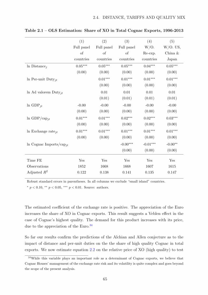
2.4. DISTANCE, TARIFFS AND QUALITY MIX
Table 2.1 – OLS Estimation: Share of XO in Total Cognac Exports, 1996-2013
(1) (2) (3) (4) (5)
Full panel
of
countries
Full panel
of
countries
Full panel
of
countries
W/O.
Re-exp.
countries
W/O. US,
China &
Japan
ln Distancej 0.05∗∗∗ 0.05∗∗∗ 0.05∗∗∗ 0.04∗∗∗ 0.05∗∗∗
(0.00) (0.00) (0.00) (0.00) (0.00)
ln Per-unit Dutyjt 0.01∗∗∗ 0.01∗∗∗ 0.01∗∗∗ 0.01∗∗∗
(0.00) (0.00) (0.00) (0.00)
ln Ad valorem Dutyjt 0.01 0.01 0.01 0.01
(0.01) (0.01) (0.01) (0.01)
ln GDPjt -0.00 -0.00 -0.00 -0.00 -0.00
(0.00) (0.00) (0.00) (0.00) (0.00)
ln GDP/capjt 0.01∗∗∗ 0.01∗∗∗ 0.02∗∗∗ 0.02∗∗∗ 0.03∗∗∗
(0.00) (0.00) (0.00) (0.00) (0.00)
ln Exchange ratejt 0.01∗∗∗ 0.01∗∗∗ 0.01∗∗∗ 0.01∗∗∗ 0.01∗∗∗
(0.00) (0.00) (0.00) (0.00) (0.00)
ln Cognac Imports/capjt -0.00∗∗∗ -0.01∗∗∗ -0.00∗∗
(0.00) (0.00) (0.00)
Time FE Yes Yes Yes Yes Yes
Observations 1852 1668 1668 1607 1615
Adjusted R2 0.122 0.138 0.141 0.135 0.147
Robust standard errors in parentheses. In all columns we exclude “small island” countries.
∗ p < 0.10, ∗∗ p < 0.05, ∗∗∗ p < 0.01. Source: authors.
The estimated coefficient of the exchange rate is positive. The appreciation of the Euro
increases the share of XO in Cognac exports. This result suggests a Veblen effect in the
case of Cognac’s highest quality. The demand for this product increases with its price,
due to the appreciation of the Euro.34
So far our results confirm the predictions of the Alchian and Allen conjecture as to the
impact of distance and per-unit duties on the the share of high quality Cognac in total
exports. We now estimate equation 2.2 on the relative price of XO (high quality) to test
34While this variable plays an important role as a determinant of Cognac exports, we believe that
Cognac Houses’ management of the exchange rate risk and its volatility is quite complex and goes beyond
the scope of the present analysis.
65
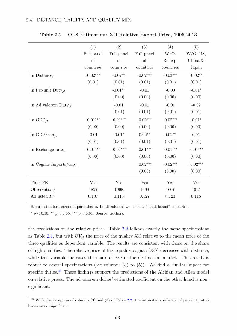
2.4. DISTANCE, TARIFFS AND QUALITY MIX
Table 2.2 – OLS Estimation: XO Relative Export Price, 1996-2013
(1) (2) (3) (4) (5)
Full panel
of
countries
Full panel
of
countries
Full panel
of
countries
W/O.
Re-exp.
countries
W/O. US,
China &
Japan
ln Distancej -0.02∗∗∗ -0.02∗∗ -0.02∗∗∗ -0.03∗∗∗ -0.02∗∗
(0.01) (0.01) (0.01) (0.01) (0.01)
ln Per-unit Dutyjt -0.01∗∗ -0.01 -0.00 -0.01∗
(0.00) (0.00) (0.00) (0.00)
ln Ad valorem Dutyjt -0.01 -0.01 -0.01 -0.02
(0.01) (0.01) (0.01) (0.01)
ln GDPjt -0.01∗∗∗ -0.01∗∗∗ -0.02∗∗∗ -0.02∗∗∗ -0.01∗
(0.00) (0.00) (0.00) (0.00) (0.00)
ln GDP/capjt -0.01 -0.01∗ 0.02∗∗ 0.02∗∗ 0.01
(0.01) (0.01) (0.01) (0.01) (0.01)
ln Exchange ratejt -0.01∗∗∗ -0.01∗∗∗ -0.01∗∗∗ -0.01∗∗∗ -0.01∗∗∗
(0.00) (0.00) (0.00) (0.00) (0.00)
ln Cognac Imports/capjt -0.02∗∗∗ -0.02∗∗∗ -0.02∗∗∗
(0.00) (0.00) (0.00)
Time FE Yes Yes Yes Yes Yes
Observations 1852 1668 1668 1607 1615
Adjusted R2 0.107 0.113 0.127 0.123 0.115
Robust standard errors in parentheses. In all columns we exclude “small island” countries.
∗ p < 0.10, ∗∗ p < 0.05, ∗∗∗ p < 0.01. Source: authors.
the predictions on the relative prices. Table 2.2 follows exactly the same specifications
as Table 2.1, but with UVjt the price of the quality XO relative to the mean price of the
three qualities as dependent variable. The results are consistent with those on the share
of high qualities. The relative price of high quality cognac (XO) decreases with distance,
while this variable increases the share of XO in the destination market. This result is
robust to several specifications (see columns (3) to (5)). We find a similar impact for
specific duties.35 These findings support the predictions of the Alchian and Allen model
on relative prices. The ad valorem duties’ estimated coefficient on the other hand is non-
significant.
35With the exception of columns (3) and (4) of Table 2.2: the estimated coefficient of per-unit duties
becomes nonsignificant.
66

2.5. CONTAINERIZATION AND QUALITY MIX
The estimated coefficient of the GDP is negative and significant. The per-capita GDP has
a less robust effect, that depends on the specifications. The effect of the exchange rate
on the relative export price of XO Cognac is consistent with our findings on the XO share.
In Table 2.7 (see appendix to chapter two) we perform another robustness check, using
an alternative estimation method: the Pseudo-Poisson-Maximum Likelihood (PPML)
method. Columns (1) and (2) report respectively the results of the share of XO exports
and their relative export prices. Our findings are qualitatively similar to those presented
in Tables 2.1 and 2.2.
2.5 Containerization and Quality Mix
Until now we have studied the impact of trade costs across countries. In this last em-
pirical section, we take interest in the effect of trade costs within countries. To do so,
we exploit the variation over time in transport costs using the historical episode of the
containerization and investigate its impact on the quality mix of Cognac exports.
2.5.1 Stylized Facts on Containerization
Maritime transport has played a key role in Cognac history starting as early as the birth
of the product itself, and later on with the establishment of regular trade links between
the French region and northern Europe in the 18th century.36 Since then, Cognac has
been and continues to be an export product. Major changes to the maritime shipping
methods and overall transport technology such as the introduction of containerization in
the 20th are unlikely to have left unaffected the international trade of Cognac.
Containerization is the method of shipping goods via containers. First introduced in the
United States in the second half of the 1950s37, containerization revolutionized trans-
portation in the 20th century. According to Bernhofen, El-Sahli, and Kneller (2016) (p.
39):
“From a transportation technology perspective, containerization resulted in the introduc-
tion of intermodal freight transport, since the shipment of a container can use multiple
modes of transportation - ship, rail or truck - without any handling of the freight when
changing modes. By eliminating sometimes as many as a dozen separate handlings of the
cargo, the container resulted in linking the producer directly to the customer.”
36Cognac was first shipped in barrels. It has been shipped in bottles from the 19th century onward.37For a detailed description and empirical analysis of the determinants of the diffusion of containeriza-
tion see Rua (2014).
67

2.5. CONTAINERIZATION AND QUALITY MIX
The overall quality of transport services improved and expenses decreased as a result of
the introduction of containerization. We are interested in studying its impact and the
resulting variation in trade costs on the Cognac quality mix.
Containerization is responsible for a reduction in the total costs of shipment from pro-
ducers to customers through different channels: improvement of dock labor productivity,
increase of shipment sizes, reduction of cargo damage and pilferage, decrease in the dura-
tion of travel journeys etc. It is however difficult to quantify the impact of containerization
on port-to-port freight costs. There is nevertheless evidence brought forward by Bern-
hofen et al. (2016) based on McKinsey’s (1972) work regarding resource savings as a
result of the adoption of containerization between 1965 and 1970/1971.38 In this respect,
the authors point out that insurance costs for a journey between Australia and Europe
dropped from “an average of 24 pennies per ton to 4 pennies per ton” (p.39). Moreover,
as a result of a significant reduction in the duration of travel journeys (from 70 to 34 days
between the two continents), the “capital cost of inventory” decreased from 2 pounds per
ton to 1 pound per ton (p. 39).
This evidence points toward a reduction of the per-unit trade costs as a result of coun-
tries entering the age of containerization. We expect therefore this technological change
to have the opposite impact of distance on the Cognac quality mix, namely a negative
effect on the share of higher quality Cognac and a positive effect on its relative price.
As previously stated, it is difficult to exactly quantify the impact of containerization on
freight costs. It is also highly likely that containerization led not only to a decrease of
per-unit trade costs, but also of ad valorem charges. Unfortunately we do not have data
on their magnitude. However, based on the information we display, we believe to be
plausible that the reduction of per-unit trade costs as a result of containerization was
relatively bigger than the reduction in the ad valorem charges.
Using Rua’s (2014) data on the years of adoption of containerization by country (i.e. when
the first port was containerized), figure 2.6 shows that the majority of Cognac importing
countries adopted containerization in the mid 1970s and beginning of the 1980s.39 The
United States was the first country to adopt containerization in 1956, while France’s first
port was containerized in 1968. The most recent adopters include: Cambodia (2003),
Vietnam (2000) and Cuba (2000).
38For further details, see Table 1, page 39 in Bernhofen et al. (2016).39A complete list of Cognac importing countries and their containerization dates is provided in the
appendix, Table 2.8.
68

2.5. CONTAINERIZATION AND QUALITY MIX
Figure 2.6 – Number of Cognac Importing Countries by Containerization Date
Source: authors; containerization dates from Rua (2014).
Figure 2.7 – Share of XO Exports Before and After Containerization
Source: authors; containerization dates from Rua (2014).
69

2.5. CONTAINERIZATION AND QUALITY MIX
In order to see if there is indeed a difference in the share of XO Cognac in total exports
after the adoption of containerization, we have a first glance at the data in figure 2.7.
We show the evolution of the average share of exports of higher quality Cognac during a
5-year period before and after the containerization. There seems to be a negative relation
between the share of XO in Cognac exports and the post-containerization period. This
would confirm the Alchian and Allen conjecture. We empirically assess this effect in the
next section.
2.5.2 Empirical Strategy and Data
Despite extensive literature on transportation economics acknowledging the change and
improvement in shipping methods brought by containerization40, there are seldom em-
pirical studies quantifying this effect, and fewer regarding the impact of containerization
on the trade of goods. A notable exception is the study by Bernhofen et al. (2016) that
estimates the impact of containerization during 1962-1990 and finds that containeriza-
tion is associated with statistically significant and larger bilateral trade whether between
North-North countries or worldwide trade.
Following the same empirical strategy as in section 2.4.2, we test the Alchian and Allen
conjecture by investigating the impact of the reduction of trade costs as a result of the
adoption of containerization on the XO share and its relative price in the country of des-
tination.
We estimate the following equation:
Zjt = β0 + β1ln(Yjt) + β2ln(yjt) + β3ln(ejt) + β4Containerjt + β5Afterjt
+ νt + νj + ujt (2.3)
Zjt is our dependent variable: (i) the share of XO in Cognac exports to country j at year
t, in volume and (ii) the price of XO exported to country j at year t, relative to the mean
price of the three qualities in j at year t. Containerjt is a dummy equal to 1 if country j
adopted containerization at year t, 0 otherwise. Afterjt is a dummy equal to 1 if country
j adopted containerization at least 1 year before t, 0 otherwise. νt and νj are time and
country fixed effects respectively. ujt is the error term.41
Note that we distinguish between the adoption date and subsequent years because con-
tainerization initially involved major changes in port facilities to accommodate this tech-
40See for example Levinson (2006).41Data on customs protection are available from 1996 to 2013, therefore we do not include the customs
protection variables when estimating equation 2.3.
70

2.5. CONTAINERIZATION AND QUALITY MIX
nological advancement. Therefore, we do not expect the impact of containerization to be
visible since the first year of adoption.
We use Rua’s (2014) data on the dates when the first ports by destination countries were
containerized to construct the containerization dummies. The rest of the independent
variables sources are the same to those explained in section 2.4.2.
Equation 2.3 is estimated for the 1969-2013 period using OLS.42 As stated in section 2.4.2,
we only keep in our panel countries that import all three qualities of Cognac at a given
year.
2.5.3 Results
Table 2.3 presents the results of our baseline equation 2.3 on the share of XO Cognac in
total exports. In the first column, the year of adoption of containerization by the first
port in the destination country has no significant impact which is not surprising. The
Afterjt dummy is significant and negative. Our predictions are therefore confirmed. The
reduction in trade costs as a result of the adoption of containerization impacts negatively
the share of the higher quality Cognac.
As we only have data on the year of containerization by the first port in destination
countries, we desegregate the Afterjt dummy in columns (2) and (3), in order to capture
more precisely after how many years the adoption of containerization has an impact.
We find a negative and significant effect on the shares of XO after three years of the
containerization of the first port and onward. This result is robust when we add the
per-capita Cognac consumption at destination countries as a control (column 3). These
results confirm our expectations and provide further empirical evidence of the Alchian
and Allen proposition.
The market size does not appear to have a significant impact on the XO share. The
impact of the GDP on the XO share is qualitatively similar to our previous results of our
baseline estimation in section 2.4.3. On the other hand, the per-capita GDP of destina-
tion countries’ impact on the XO share depends on the specification. The exchange rate
has no significant impact on the share of XO Cognac.
In columns (4) to (6) we perform several robustness checks. In column (4) we use an alter-
native source for the containerization dates based on Bernhofen et al. (2016). They cover
42France’s first port was containerized in 1968, therefore we exclude from our panel the 1967 and 1968
Cognac trade data.
71

2.5. CONTAINERIZATION AND QUALITY MIX
Table 2.3 – OLS Estimation: Share of XO in Total Cognac Exports, 1969-2013
(1) (2) (3) (4) (5) (6)
Full
panel of
countries
Full
panel of
countries
Full
panel of
countries
Bernhofen
& al.
(2016)
W/O.
re-export.
countries
W/O.
U.S.,
China &
Japan
Container.jt -0.01 -0.01 -0.01 -0.04 -0.01 -0.03∗
(0.02) (0.02) (0.02) (0.02) (0.02) (0.02)
Afterjt -0.04∗∗∗
(0.01)
1Y after container.jt -0.02 -0.02 -0.03 -0.03 -0.03∗
(0.02) (0.02) (0.02) (0.02) (0.02)
2Y after container.jt -0.01 -0.01 -0.03 -0.01 -0.02
(0.02) (0.02) (0.02) (0.02) (0.02)
3Y after container.jt -0.06∗∗∗ -0.06∗∗∗ -0.04∗∗ -0.06∗∗∗ -0.06∗∗∗
(0.02) (0.02) (0.02) (0.02) (0.02)
4Y after container.jt -0.05∗∗∗ -0.05∗∗∗ -0.05∗∗∗ -0.05∗∗∗ -0.06∗∗∗
(0.02) (0.02) (0.02) (0.02) (0.01)
5+Y after container.jt -0.05∗∗∗ -0.05∗∗∗ -0.06∗∗∗ -0.05∗∗∗ -0.06∗∗∗
(0.01) (0.01) (0.01) (0.01) (0.01)
ln GDPjt 0.01 0.01 -0.00 0.01 0.01 -0.00
(0.02) (0.02) (0.02) (0.02) (0.02) (0.02)
ln GDP/capjt -0.06∗∗∗ -0.06∗∗∗ -0.02 -0.04 -0.03 -0.02
(0.02) (0.02) (0.02) (0.02) (0.02) (0.02)
ln Exchange ratejt -0.00 -0.00 0.00 0.00 0.00 0.00
(0.00) (0.00) (0.00) (0.00) (0.00) (0.00)
ln Tot Cognac Imp./capjt -0.01∗∗∗ -0.01∗∗∗ -0.01∗∗∗ -0.01∗∗∗
(0.00) (0.00) (0.00) (0.00)
Time FE Yes Yes Yes Yes Yes Yes
Country FE Yes Yes Yes Yes Yes Yes
Observations 2793 2793 2793 2429 2682 2662
Adjusted R2 0.481 0.482 0.487 0.504 0.450 0.496
Robust standard errors in parentheses. In all columns we exclude “small island” countries.∗ p < 0.10, ∗∗ p < 0.05, ∗∗∗ p < 0.01. Source: authors.
countries that have containerized up until 1983.43 A full list of countries and their con-
43The two databases differ in the years of adoption of containerization for almost half of the Cognac
importing countries. These differences are probably due to data sources. Rua (2014) constructs her
database based on the: Containerisation International Yearbook, Shipping Statistics Yearbook and Lloyd’s
Ports of the World. Bernhofen et al. (2016) mention gathering information “scattered in transportation
industry journals” (p. 36).
72

2.5. CONTAINERIZATION AND QUALITY MIX
Table 2.4 – OLS Estimation: XO Relative Export Price, 1969-2013
(1) (2) (3) (4) (5) (6)
Full
panel of
countries
Full
panel of
countries
Full
panel of
countries
Bernhofen
& al.
(2016)
W/O.
re-export.
countries
W/O.
U.S.,
China &
Japan
Container.jt 0.01 0.02 0.02 0.05 0.02 0.02
(0.03) (0.03) (0.03) (0.04) (0.03) (0.03)
Afterjt 0.04∗
(0.02)
1Y after container.jt -0.01 -0.00 0.01 -0.00 -0.01
(0.03) (0.03) (0.03) (0.03) (0.03)
2Y after container.jt 0.02 0.02 0.08∗∗ 0.03 0.02
(0.04) (0.04) (0.03) (0.04) (0.04)
3Y after container.jt 0.04 0.04 0.06∗ 0.04 0.04
(0.03) (0.03) (0.03) (0.03) (0.03)
4Y after container.jt 0.04 0.04 0.05 0.05 0.04
(0.03) (0.03) (0.03) (0.03) (0.03)
5+Y after container.jt 0.06∗∗ 0.07∗∗∗ 0.11∗∗∗ 0.08∗∗∗ 0.06∗∗
(0.03) (0.03) (0.03) (0.03) (0.03)
ln GDPjt -0.03 -0.04 -0.02 0.00 -0.02 -0.06
(0.04) (0.04) (0.04) (0.05) (0.04) (0.04)
ln GDP/capjt 0.01 0.02 -0.04 -0.05 -0.04 -0.00
(0.04) (0.04) (0.04) (0.05) (0.05) (0.04)
ln Exchange ratejt 0.00 0.00 0.00 -0.00 0.00 -0.00
(0.00) (0.00) (0.00) (0.00) (0.00) (0.00)
ln Tot Cognac Imp./capjt 0.02∗∗∗ 0.02∗∗∗ 0.02∗∗∗ 0.02∗∗∗
(0.01) (0.01) (0.01) (0.01)
Time FE Yes Yes Yes Yes Yes Yes
Country FE Yes Yes Yes Yes Yes Yes
Observations 2793 2793 2793 2429 2682 2662
Adjusted R2 0.604 0.605 0.607 0.615 0.600 0.626
Robust standard errors in parentheses. In all columns we exlude “small island” countries.∗ p < 0.10, ∗∗ p < 0.05, ∗∗∗ p < 0.01. Source: authors.
tainerization dates is provided in the appendix 2.D. Our results are robust. In columns
(5) and (6) we exclude from our panel re-exporting countries and the US, Japan and
China, respectively. Our main finding is unaltered: post-containerization has impacted
negatively the shares of higher quality Cognac, providing further empirical evidence of
the validity of the Alchian and Allen conjecture.
73

2.6. CONCLUSION
Table 2.4 shows the results of our estimation of equation 2.3 on the relative price of the
higher quality Cognac. Post-containerization (column 1) has a positive impact on the
relative price of XO which is in line with our predictions. By decomposing the Afterjt
dummy variable, we find that the impact on the relative price becomes apparent start-
ing 5 years after the containerization. This result is unaltered when we control for the
per-capita Cognac consumption at destination countries (column 3). Our results with
respect to the impact of the adoption of containerization on the relative price of higher
quality Cognac are overall in line with our results of its impact on the share of XO Cognac.
Our robustness tests shown in columns (4) to (6) confirm our previous findings. Con-
tainerization has a positive impact on the relative price of XO Cognac starting from 5
years after its adoption. When we use the Bernhofen et al. (2016) database, the effect
is present starting from three years after the initial adoption. This result confirms our
predictions.
In Table 2.9 in the appendix to chapter two we perform further robustness checks, using
the PPML estimation method and find qualitatively similar results.
2.6 Conclusion
Using a unique database of annual Cognac shipments by volume, destination and quality
designations, we test empirically the validity of Alchian and Allen’s thesis according to
which per-unit transportation costs increase the relative demand for higher quality goods.
We test empirically the impact of trade costs on the share of higher quality (XO) Cognac
and its relative price. First, we evaluate the impact of trade costs (distance and customs
protection) across countries. Second, we investigate the effect of the variation in trade
costs within countries as per the adoption of containerization. Our results validate the
Alchian and Allen effect meaning that per-unit trade costs increase the relative demand
of higher quality Cognac.
In the introduction to this chapter we stated that Cognac is a luxury product. We show
that the Alchian and Allen effect is present even for a luxury product.
An object of our future consideration is to obtain producing firms’ data and analyze
their strategies and the determinants of their export performance. It would allow us to
examine if the Alchian and Allen effect is due to cross-firm selection (only firms that
produce higher quality goods export to more distant markets) or within-firm selection
(firms choose higher quality and more expensive goods when they decide to export to
more distant markets).
74

Appendix to Chapter 2
2.A General Framework: Mathematical Proofs
2.A.1 The Alchian and Allen Effect in a Two-Good World
Proof of equation 2.1:
∂(XjH/XjL)
∂tj=
∂XjH
∂tjXjL −XjH
∂XjL
∂tj
X2jL
(2.4)
From the chain rule we have:
∂Xjk
∂tj=∂Xjk
∂pjH+∂Xjk
∂pjLk = H,L.
Substituting into (2.4):
∂(XjH/XjL)
∂tj=
(∂XjH
∂pjH+
∂XjH
∂pjL)XjL −XjH(
∂XjL
∂pjH+
∂XjL
∂pjL)
X2jL
<=>
∂(XjH/XjL)
∂tj=
(εHHXjH
pjH+ εHL
XjH
pjL)XjL −XjH(εLH
XjL
pjH+ εLL
XjL
pjL)
X2jL
, with εkm =∂Xjk
∂pjk
pjkXjk
<=>
∂(XjH/XjL)
∂tj=XjH
XjL
(εHHpjH
+εHLpjL− εLHpjH− εLLpjL
) (2.5)
From Hick’s third law (1946, p. 310-311) for two goods:∑2
n=1 εln = 0, l = 1, 2. Substi-
tuting εHH with and −εHL and −εLH with εLL into (2.5), we have:
∂(XjH/XjL)
∂tj=XjH
XjL
(−εHLpjH
+εHLpjL
+εLLpjH− εLLpjL
)
<=>
∂(XjH/XjL)
∂tj=XjH
XjL
(1
pjL− 1
pjH)(εHL − εLL) (2.6)
75

2.A. GENERAL FRAMEWORK: MATHEMATICAL PROOFS
The term 1pjL− 1
pjHin (2.6) is positive because piH > piL.
Indeed, piH > piL <=> piH + tj > piL + tj => pjH > pjL <=> 1pjH
< 1pjL
As long as XjH and XjH are close substitutes, εHL > 0. Given that the own price-elasticity
εLL < 0, the term εHL−εLL > 0, therefore∂(XjH/XjL)
∂tj> 0, verifying the Alchian and Allen
effect.
Now consider that prices at destination country j depend on prices at origin country i
and a per-value charge dj such as:
pjk = pik ∗ dj, k = H,L.
We study how a change in dj impacts the relative demandXjH
XjL.
Following the same mathematical steps of the demonstration above, we have:
∂(XjH/XjL)
∂dj=XjH
XjL
(piLpjL− piHpjH
)(εHL − εLL) (2.7)
The term in the middle piLpjL− piH
pjHis equal to zero. Proof:
piLpjL− piHpjH
=piLpjH − piHpjL
pjLpjH=piLpiH ∗ dj − piHpiL ∗ dj
pjLpjH= 0
Consequently,∂(XjH/XjL)
∂dj= 0. For all else equal, the Alchian and Allen conjecture does
not hold when an ad valorem charge (e.g. an “iceberg” transport cost or ad valorem duty)
is added to the prices of the high and low quality goods.
2.A.2 The Alchian and Allen Effect in a Three-Good World
Let us suppose now that the demand for the high and low quality good at destination
country j depends not only on pjH and pjL, but also on the price of a composite good
(i.e. Hicksian good) denoted by pjC44, such as:
Xjk = f(pjH , pjL, pjC , U), k = H,L.
From equation 2.5 and Hicks’ third law for three goods:∑3
n=1 εln = 0, l = 1, 2, 3, we have:
∂(XjH/XjL)
∂tj=XjH
XjL
(−εHL − εHC
pjH+εHLpjL
+εLL + εLC
pjH− εLLpjL
)
44A composite good represents “all other goods”: “If the prices of a group of goods change in the same
proportion, than that group of goods behaves as if it were a single commodity” (Hicks, 1946, p. 313).
76

2.A. GENERAL FRAMEWORK: MATHEMATICAL PROOFS
<=>
∂(XjH/XjL)
∂tj=XjH
XjL
[(1
pjL− 1
pjH)(εHL − εLL) +
1
pjH(εLC − εHC)] (2.8)
The sign of∂(XjH/XjL)
∂tjdepends on the sign of (εLC − εHC). The sign of the rest of the
terms in brackets is positive as previously demonstrated.
Borcherding and Silberberg (1978) argue that if the two quality grades of the same good
are close substitutes, “there is little reason to presume that their interactions with the
composite commodity should be widely disparate” (p. 135). Therefore, εLC − εHC tends
to zero and∂(XjH/XjL)
∂tj> 0, verifying the Alchian and Allen effect.
77

2.B. STYLIZED FACTS: MAIN MARKETS
2.B Stylized facts: Main Markets
Table 2.5 – Descriptive Statistics - Share of XO in Imports of Main Markets
Share in Share in
total exports XO exports Nb. Obs. mean sd min max
Total - - 2842 13.64 14.47 0.01 95.01
USA 32.20 8.80 22 3.37 1.26 1.89 7.22
Singapore 17.62 27.54 22 27.48 6.36 18.98 39.08
China 12.66 28.24 22 34.94 15.69 10.16 73.42
UK 6.43 0.71 22 1.53 0.18 1.22 2.00
Germany 3.73 2.54 22 5.63 2.14 2.20 9.50
Hong Kong 2.93 9.93 22 38.80 9.19 17.93 53.78
Netherlands 2.27 1.11 22 4.73 1.87 1.89 7.92
Norway 1.73 2.75 22 18.12 7.93 2.13 26.05
Finland 1.42 1.11 22 11.21 4.44 6.16 23.68
Russia 1.33 0.94 22 12.25 4.56 2.43 22.23
Latvia 1.30 1.02 21 11.42 5.71 1.15 27.46
Malaysia 1.04 3.72 22 29.50 12.33 12.98 49.93
Nigeria 1.03 0.19 22 1.96 0.95 0.38 4.36
Ireland 0.93 0.01 22 0.25 0.08 0.11 0.44
Canada 0.89 0.43 22 6.68 1.21 3.66 8.46
Table 2.6 – Descriptive Statistics - Share of VS in Imports of Main Markets
Share in Share in Share of VS
total exports VS exports Nb. Obs. mean sd min max
Total - - 2842 45.22 27.57 0.00 99.57
USA 32.20 50.61 22 74.56 2.92 69.72 79.97
Singapore 17.62 3.52 22 1.95 2.15 0.32 8.89
China 12.66 2.16 22 8.30 16.41 0.00 71.15
UK 6.43 12.35 22 86.42 1.69 81.99 89.03
Germany 3.73 4.11 22 56.45 5.05 47.60 63.03
Hong Kong 2.93 0.26 22 1.75 1.07 0.64 3.99
Netherlands 2.27 2.33 22 60.59 8.93 45.54 74.46
Norway 1.73 1.62 22 51.47 9.65 35.19 66.01
Finland 1.42 1.93 22 60.82 3.52 53.90 67.71
Russia 1.33 1.62 22 37.00 11.62 8.24 55.01
Latvia 1.30 1.28 21 39.64 10.15 7.84 51.06
Malaysia 1.04 0.01 22 0.60 0.38 0.18 1.62
Nigeria 1.03 1.42 22 34.36 19.93 0.02 67.00
Ireland 0.93 2.07 22 97.96 0.60 96.68 98.96
Canada 0.89 1.35 22 65.40 4.88 51.57 73.35
78

2.B. STYLIZED FACTS: MAIN MARKETS
Figure 2.8 – Share of VS in Cognac’s Imports by Country, 2013
[0,20]
(20,40]
(40,60]
(60,80]
(80,100]
No data
Source: authors; raw data from BNIC.
Figure 2.9 – Share of VS in Cognac’s Exports According to Distance, 2013
Source: authors; raw data from BNIC.
79

2.C. DISTANCE, TARIFFS AND QUALITY MIX: AN ADDITIONAL TEST
2.C Distance, Tariffs and Quality Mix: An Addi-
tional Test
Table 2.7 – Alternative Estimation Method: PPML, 1996-2013
(1) (2)
XO Sharejt XO UVjt
ln Distancej 0.37∗∗∗ 0.37∗∗∗
(0.02) (0.02)
ln Per-unit Dutyjt 0.04∗∗∗ 0.04∗∗∗
(0.01) (0.01)
ln Ad valorem Dutyjt 0.07 0.07
(0.05) (0.05)
ln GDPjt -0.02∗ -0.02∗
(0.01) (0.01)
ln GDP/capjt 0.14∗∗∗ 0.14∗∗∗
(0.03) (0.03)
ln Exchange ratejt 0.06∗∗∗ 0.06∗∗∗
(0.01) (0.01)
ln Cognac Imports/capjt -0.03∗∗ -0.03∗∗
(0.01) (0.01)
Time FE Yes Yes
Observations 1668 1668
Robust standard errors in parentheses.
In both columns we exclude “small island” countries.
∗ p < 0.10, ∗∗ p < 0.05, ∗∗∗ p < 0.01. Source: authors.
80

2.D. CONTAINERIZATION: DATABASES
2.D Containerization: Databases
Table 2.8 – Adoption of Containerization (First Port Containerized) by Cognac
Importing Countries
Country Name Containerization Date Containerization Date
(Rua, 2014) (Bernhofen et al., 2016)
Algeria 1979 1979
Angola 1979 1979
Argentina 1977 1976
Aruba 1976
Australia (and Papua New Guinea) 1964 1968
Austria 1982 1968 (*)
Bahamas 1972 1973
Bahrain 1977 1977
Bangladesh 1981 1981
Belgium (and Luxembourg) 1966 1968
Belize 1981 1981
Benin 1976 1976
Bermuda 1983 1983
Brazil 1971 1973
Bulgaria 1972 1972 (R)
Cambodia 2003
Cameroon 1973 1974
Canada 1968 1968
Cayman Islands 1998
Chile 1973 1974
China 1979 1979
Colombia 1971 1974 (R)
Congo 1979 1979
Congo, Democratic Republic of the 1981 1981
Costa Rica 1980 1981
Cote d’Ivoire 1970 1971
Cuba 2000
Cyprus 1977 1977
Denmark 1969 1968
Djibouti 1979 1979
Dominican Republic 1976 1981
Bernhofen et al. (2016) database reports the dates of containerization by port or rail, whichever took place first.
Countries marked with (R) containerized by rail first and are dropped from the estimations. Countries marked with (*)
also containerized by rail first. Because the adoption occurred before port containerization comparing it to Rua’s (2014)
data, we substitute the latter to the former date.
81

2.D. CONTAINERIZATION: DATABASES
Adoption of Containerization (First Port Containerized) by Cognac Importing
Countries (Continued)
Country Name Containerization Date Containerization Date
(Rua, 2014) (Bernhofen et al., 2016)
Ecuador 1970 1978
Egypt 1978 1978
El Salvador 1978 1979
Ex-Czechoslovakia 1979 1972 (*)
Ex-Yugoslavia 1970 1969 (*)
Finland 1970 1969
Former URSS 1971 1970 (R)
French Polynesia 1978
Gambia 1982 1982
Germany 1968 1966
Ghana 1978 1977
Gibraltar 1978 1978
Greece 1971 1970
Guatemala 1976 1980
Guinea 1983 1983
Haiti 1976 1978
Honduras 1975 1975
Hong Kong 1970 1970
Hungary 1969 1968 (*)
Iceland 1973 1973
India 1971 1966 (*)
Indonesia 1975 1975
Iran, Islamic Republic of 1977 1977
Iraq 1977 1978
Ireland 1967 1968 (R)
Israel 1970 1970
Italy 1968 1968
Jamaica 1969 1973
Japan 1968 1969
Jordan 1976 1977
Kenya 1975 1976
Korea, Republic of 1975 1975
Kuwait 1977 1977
Lebanon 1977 1977
Liberia 1980 1980
Libya 1979 1980
Madagascar 1980 1980
Malta 1979 1983
Mauritania 1982 1982
Mexico 1976 1976
Morocco 1977 1977
Mozambique 1975 1978
Myanmar 1982 1983
Bernhofen et al., 2016 database reports the dates of containerization by port or rail, whichever took place first.
Countries marked with (R) containerized by rail first and are dropped from the estimations. Countries marked with (*)
also containerized by rail first. Because the adoption occurred before port containerization comparing it to Rua’s (2014)
data, we substitute the latter to the former date.
82

2.D. CONTAINERIZATION: DATABASES
Adoption of Containerization (First Port Containerized) by Cognac Importing
Countries (Continued)
Country Name Containerization Containerization
(Rua, 2014) (Bernhofen et al., 2016)
Netherlands 1966 1966
Netherlands Antilles 1979 1979
New Caledonia 1981 1976
New Zealand 1967 1971
Nicaragua 1977 1979
Nigeria 1967 1974
Norway 1968 1969 (R)
Pakistan 1980 1979
Panama 1976 1974 (*)
Peru 1969 1975
Philippines 1971 1971
Poland 1970 1971
Portugal 1970 1969
Qatar 1979 1979
Romania 1981 1970 (*)
Samoa 1981 1978
Saudi Arabia 1976 1976
Senegal 1985
Sierra Leone 1978 1978
Singapore 1969 1970
South Africa 1971 1974
Spain 1967 1968 (R)
Sudan 1979 1980
Sweden 1968 1968 (R)
Switzerland 1968 1968 (R)
Syrian Arab Republic 1979 1979
Taiwan, Province of China 1969 1968
Tanzania, United Republic of 1975 1978
Thailand 1975 1975
Togo 1981 1981
Trinidad and Tobago 1973 1971
Tunisia 1981 1981
Turkey 1981 1981
United Kingdom 1966 1966
United States 1956 1966
Uruguay 1980 1980
Vanuatu 1978
Venezuela, Bolivarian Republic of 1981 1981
Viet Nam 2000
Yemen 1978
Bernhofen et al., 2016 database reports the dates of containerization by port or rail, whichever took place first.
Countries marked with (R) containerized by rail first and are dropped from the estimations. Countries marked with (*)
also containerized by rail first. Because the adoption occurred before port containerization comparing it to Rua’s (2014)
data, we substitute the latter to the former date.
83

2.E. CONTAINERIZATION AND QUALITY MIX: AN ADDITIONAL TEST
2.E Containerization and Quality Mix: An Additional
Test
Table 2.9 – Alternative Estimation Method: PPML, 1969-2013
(1) (2)
XO Sharejt XO UVjt
Containerizationjt -0.14 0.04∗
(0.13) (0.02)
1Y after container.jt -0.16 0.01
(0.11) (0.02)
2Y after container.jt -0.11 0.06∗∗
(0.11) (0.02)
3Y after container.jt -0.22∗∗ 0.04∗
(0.10) (0.02)
4Y after container.jt -0.25∗∗∗ 0.03
(0.09) (0.02)
5+Y after container.jt -0.33∗∗∗ 0.08∗∗∗
(0.08) (0.02)
ln GDPjt 0.22∗ -0.01
(0.13) (0.03)
ln GDP/capjt -0.16 -0.01
(0.16) (0.03)
ln Exchange ratejt 0.00 -0.00
(0.01) (0.00)
ln Tot Cognac Imports/capjt -0.06∗∗∗ 0.01∗∗∗
(0.02) (0.00)
Time FE Yes Yes
Country FE Yes Yes
Observations 2429 2429
Robust standard errors in parentheses.
In both columns we exclude “small island” countries.
∗ p < 0.10, ∗∗ p < 0.05, ∗∗∗ p < 0.01. Source: authors.
84

Chapter 3
Vertical Differentiation, Uncertainty,
Product R&D and Policy
Instruments in a North-South
Duopoly1
3.1 Introduction
In the aftermath of the global economic crisis from which many developed and developing
countries have still not fully recovered, decision makers’ attention is increasingly drawn
to structural reforms needed to raise their countries’ competitiveness as one of the main
drivers of economic prosperity.2 Determining and implementing the right policies to im-
prove competitiveness is a challenging issue and so it has been for years, especially in
high-income economies facing growing competition from low-income ones.
According to the Global Competitiveness Report for 2014-2015, economies which have
successfully managed to stay the most competitive “are able to develop...and constantly
introduce new and higher value-added products and services into the market” (see Key
Findings, Smart Investing). Countries such as Switzerland, Singapore, the United States,
Finland, Germany are ranked among the most competitive.3 Not surprisingly, the ma-
1This chapter is a substantially revised version of the LAREFI Working Paper N. 2016-02, jointly
written with Julien Berthoumieu (Berthoumieu and Lamani, 2016). It has been submitted for publication
in the Canadian Journal of Economics.2Competitiveness (in international trade) may be defined as a measure of a country’s advantage or
disadvantage in selling its products on international markets (OECD).3This ranking is based on the Global Competitiveness Index, developed by the World Economic
Forum. The rest of the countries in the top ten of most competitive economies are: Japan, Hong Kong,
the Netherlands, the United Kingdom and Sweden.
85

3.1. INTRODUCTION
jority of these economies have registered the highest Research and Development (R&D)
expenditures as percentage of GDP.4 Process and/or product innovation5 are therefore
among the key factors to achieve economic growth.
Investing in R&D contributes to the improvement of firms’ competitiveness and their
export performance. Determining whether a country’s government can support its do-
mestic firms’ innovation activities is an important issue. Indeed, as mentioned in the
introduction to chapter two, it is well established in the theoretical literature and well
supported by empirical evidence that countries trade in similar (horizontally and/or ver-
tically differentiated) products.6 In this respect, product innovation induced by product
R&D investment, influences features of finished goods, such as quality. Investing in R&D
and producing higher quality goods is a way for firms, especially in high-income countries,
to counter growing competition from developing countries with a cost-competitive advan-
tage. Firms’ product R&D activities may however be affected by policy-related costs such
as customs barriers.
The objective of this chapter is to develop a theoretical model and evaluate the impact
of several and different trade policy instruments on product R&D investment. We also
examine the impact of these instruments on firms’ profits, consumer surplus, public rev-
enues. We also conduct a welfare analysis.
Extensive theoretical studies focus on the impact of trade policy instruments on cost-
reducing (process) R&D (Bhagwati, 1968; Krishna, 1989; Reitzes, 1991). Theoretical
examinations of product R&D and vertical differentiation, concentrate primarily on iden-
tifying strategic product R&D policies (Park, 2001; Jinji, 2003; Jinji and Toshimitsu,
2006; Ishii, 2014). Furthermore, most of these analyses consider the R&D activity to
have a certain outcome, that is to say that process R&D investment, for example, reduces
marginal cost with certainty. In our study we explore the impact of both traditional (an
import tariff and an import quota) and more modern (a quality standard) trade policy
instruments on product R&D investment and welfare. We follow Bouet (2001) and intro-
duce uncertainty in the modeling of the R&D activity. We believe it yields more realistic
results.
We design a framework with a North-South duopoly where firms with asymmetric pro-
4Source: World Bank’s WDI.5Process innovation involves “significant changes in techniques, equipment and/or software” that lead
to the “implementation of a new or significantly improved production or delivery method.” Product
innovation is “introduction of a good or service that is new or significantly improved with respect to its
characteristics or intended uses (OECD).”6See for example: Falvey (1979), Krugman (1979) and Lancaster (1980).
86

3.1. INTRODUCTION
duction costs compete in prices on both markets. We assume that the Northern country’s
government is the only one to be policy active. The Northern firm bears higher production
costs and has an incentive to invest in product R&D. The outcome of this investment is
uncertain. There exists a probability of success. If successful, the Northern firm produces
a higher quality version of the same good compared to its Southern competitor. If the
Northern firms’ R&D outcome is unsuccessful, then no quality improvement is imple-
mented and the goods are horizontally differentiated due to their different cost structure.
Our model involves a three-stage game. First, the Northern firm’s government selects the
optimal instrument level by anticipating the Northern firm’s product R&D investment
and levels of price. Second, the Northern firm decides on the product R&D expendi-
tures that maximize its expected profit. In the final stage, firms set their price levels.
Our framework relates to the automobile industry, for example, in which Northern firms
invest in product R&D in order to face growing competition from Southern firms that
benefit from lower production costs.
In this chapter, we study the impact of the implementation of an import tariff, an import
quota and a quality standard by the Northern government on the domestic product R&D.
Traditional forms of instruments such as tariffs and quotas represented less than half of
all implemented measures in 2013 (Evenett, 2013). However, in the automobile industry
for example, the European Union’s ad valorem import tariff in 2014 amounted to ten
percent.7 Moreover, many developed countries still implement import quotas in the auto-
mobile industry. The number of quantitative restrictions in force on automobile vehicles
imports in 2015 is 18 in Australia, 6 in Canada, 4 in the European Union, 12 in Japan, 8
in New-Zealand, and 7 in Switzerland.8 Quality standards, are on the contrary, modern
policy instruments. A good example in the automobile industry is the implementation of
the ISO technical specification ISO/TS 16949 aimed at quality improvement and defect
prevention.
The main finding of our analysis is that the import tariff and the quality standard in-
crease the Northern firm’s R&D expenditures while the import quota decreases them.9
Therefore, a government whose only aim is to enhance non-price competitiveness by en-
couraging product R&D investments should implement one of these policy instruments.
Nevertheless, the latter may have opposite effects on the expected consumer surplus, pub-
7Source: MAcMap HS6.8Source: WTO.9The positive impact of policy instruments such as subsidies or tax cuts on the R&D investment has
been illustrated in empirical studies: Mansfield (1986), Berger (1993) and Hall (1993) - for US firms;
Mansfield and Switzer (1985) and Bernstein (1986) - for Canadian firms; Mansfield (1986) - for Swedish
firms; and Bloom et al., (2002) - for nine OECD countries.
87

3.2. REVIEW OF LITERATURE
lic revenues and welfare. We illustrate this result through numerical simulations.
The contribution of our work is twofold. First, we develop a theoretical framework and
analyze the impact of several trade policy instruments on product R&D investment. It is
an issue that has been less well-studied in the literature. Second, we consider the outcome
of such an investment to be uncertain. Vertical differentiation only occurs if the R&D
activity is successful.
The rest of this chapter is organized as follows. Section 3.2 reviews the literature. Section
3.3 describes the theoretical model. Section 3.4 presents an example under linear demand
functions. Section 3.5 analyzes the impact of two traditional policy instruments on the
Northern firms’ R&D investment: an import tariff and an import quota. Section 3.6
analyzes the impact of a modern policy instrument: a quality standard. Section 3.7
conducts a welfare analysis and compares the efficiency of the policy instruments. Section
3.8 illustrates an extension with a non-prohibitive quality standard. Section 3.9 concludes.
3.2 Review of Literature
The economic literature focusing on cost-reducing/process R&D and product R&D is
extensive. It has been shown empirically that firms invest in both product and process
R&D (Capon et al., 1992; Landau and Rosenberg, 1992). Studies show that firms invest
in product R&D at the beginning of a product’s lifecycle, and invest in process R&D at
the end (Utterback and Abernathy, 1975; Klepper, 1996). It explains why firms invest
more in product R&D (Chenavaz, 2011). We, however, focus on product R&D, which
is more important than process R&D in countries such as Germany, the United States,
and Japan according to empirical data (Fritsch and Meschede, 2001; Nagaoka and Walsh,
2009).10 Product R&D is particularly more prevalent than process R&D in high-tech
industries like automobile or electricity (Scherer and Ross, 1990; Fritsch and Meschede,
2001; Park, 2001; Toshimitsu, 2003; Jinji and Toshimitsu, 2013).
Early theoretical studies with product R&D examining firms’ choices of product quality
include Mussa and Rosen (1978) and Shaked and Sutton (1982). Mussa and Rosen (1978)
compare the quality levels under two market structures - monopoly and competition - and
conclude that producers sell lower quality goods under the former market structure than
the latter. This result explains why the cost for consumers under monopoly increases with
their taste for quality. Prices are also higher under monopoly. Shaked and Sutton (1982)
10Fritsch and Meschede (2001) note that product R&D accounts for 61 percent of all R&D expenditures
for German firms. Nagaoka and Walsh (2009) show that process innovations accounted for only 25 percent
and 17 percent of all R&D projects in the US and Japan respectively.
88

3.2. REVIEW OF LITERATURE
develop a theoretical model in which firms set first the optimal level of quality, and then
the optimal level of price. Under duopoly firms select different quality levels, while they
select the same level when the number of firms is greater than two.
There are relatively few studies related to our analysis (Park, 2001; Zhou, Spencer, and
Vertinsky, 2002; Jinji, 2003; Jinji and Toshimitsu, 2006; Jinji and Toshimitsu, 2013; Ishii,
2014). These authors develop theoretical models of international trade with vertically-
differentiated products. Their main objective is to identify optimal strategic product
R&D policies.11
Park (2001) designs a duopoly with a high- and a low-tech firm. They compete in Bertrand
or Cournot fashion on a third market. They produce vertically-differentiated products,
whose quality is determined endogenously through product R&D investment.12 The main
result of the paper is that the governments’ incentives targeting their domestic firms’ R&D
activities depend on the nature of market competition. Under Bertrand competition,
the optimal strategic policy is to tax (respectively subsidize) the high-tech (respectively
low-tech) firm’s product R&D. Results are reversed in case of Cournot competition. Fur-
thermore, the author briefly discusses the case where different instruments are combined
to serve the high-tech firm’s government strategic policy. A combination of an export
subsidy and an R&D tax is demonstrated to be optimal.
The model of Zhou, Spencer, and Vertinsky (2002) is very similar to Park (2001) in its
framework and results regarding unilateral optimal strategic product R&D policies. They
extend the analysis by examining the governments’ incentives when there is policy coor-
dination between the two countries. The authors find that when firms compete in prices,
the jointly optimal policy is to subsidize (tax) product R&D activities of the high-quality
(low-quality) producing firm. Under Cournot competition on the other hand, the optimal
policy is to implement an R&D tax in both countries. Nevertheless, empirical examples of
R&D taxes are scarce (Audretsch and Yamawaki, 1988; Gabriele, 2002; Impullitti, 2010).
While both of these papers’ analyses apply to competition between firms with large asym-
metries in R&D costs, as it is the case for firms from developed and developing countries,
Jinji (2003) studies strategic product R&D policy choices in a third-market trade model
11The economic literature also studies the case of vertical differentiation under an asymmetric frame-
work between a high-tech firm from a rich country and a low-tech firm from a developing country (Das
and Donnenfeld, 1989; Park, 2001; Zhou, Spencer, and Vertinsky, 2002; Moraga-Gonzalez and Viaene,
2005; Ishii, 2014).12Park (2001) assumes that the difference in terms of product R&D costs between firms is large enough
so that firms with lower quality improvement costs (high-tech firms) produce and export higher-quality
goods compared to low-tech competitors.
89

3.3. GENERAL FRAMEWORK
in which domestic and foreign firms are identical, facing the same product R&D costs.
In his vertically-differentiated duopoly framework, the author shows that governments’
optimal strategies involve different subsidy/tax schedules which depend on the mode of
competition. This result is qualitatively similar to Park (2001) and Zhou et al. (2002)
except for the high quality exporter’s identity which is undetermined. Either firm can
produce and export the high quality good, so that its government will choose to tax or
subsidize its product R&D investment accordingly.
Meanwhile, Jinji and Toshimitsu (2006) study strategic product R&D policies when firms
have asymmetric R&D costs. Their analysis differs from Park (2001) and Zhou et al.
(2002) since a small technology gap between firms is assumed. The quality ordering is
endogenously determined. The firm with superior technology produces the high quality
good, while its competitor produces the low quality one. This is achieved by implement-
ing a firm-specific subsidy schedule that depends on the nature of market competition.
Jinji and Toshimitsu (2013) extend previous studies by including a third exporting firm
(and country) in their model. Firms export their entire production to a fourth country.
They have different R&D capabilities, but their R&D cost functions are identical as long
as their products qualities are below their R&D capabilities. Contrary to earlier studies,
the authors find that the optimal strategic R&D policy is influenced by the nature of
market competition only in the case of the high-quality exporter. Governments of middle
and low-quality exporters would respectively tax and subsidize their domestic firm’s R&D
under both price and quantity competition. If firms coordinate, the joint optimal R&D
policies differ depending on the countries’ coordination pairs and mode of competition.
Finally, Ishii (2014) develops a theoretical third-country trade model of price competition
with less stringent demand and cost functions. He finds that the optimal R&D policy
does not only necessarily depend on the mode of competition, given that in certain sit-
uations, both governments’ optimal policy involves a product R&D subsidy even when
firms compete in Bertrand fashion.
3.3 General Framework
We develop a theoretical model of international trade with product innovation in a North-
South duopoly with a firm from a Northern country and another from a Southern country.
Each firm sells one share of its output domestically and exports the other share to the
foreign market. The Southern firm has a cheaper labor force compared to its competitor.
Assuming that the Northern firm is located in a developed country, while its Southern
trade partner is from an emerging country, considering that the latter has lower labor costs
90

3.3. GENERAL FRAMEWORK
is not unrealistic. The Northern firm has an incentive to invest in R&D and vertically
differentiate its product since the Southern firm benefits from a competitive advantage.
Our theoretical framework relates to an empirical example, for instance the mobile phone
industry. In the past decade handset manufacturing firms from Northern countries which
continue to export their finished goods to foreign markets, have been facing growing
competition even in their local markets from firms in emerging countries. Indeed, while
Seoul-based Samsung and California-based Apple continue to dominate the worldwide
smartphone industry in the third quarter of 2016, as they have in the past couple of
years, the remaining players in the top-five are Chinese companies: Huawei, OPPO, and
vivo (International Data Corporation, IDC). While OPPO’ and vivo’s increasing market
shares are driven by sales to local and other emerging markets, Huawei has successfully
penetrated developed country markets, especially in Europe.13 The company, whose own
smartphone brand has been on the markets for less than ten years, attracted customers
with its cheaper prices according to the Financial Times.14 Although Huawei has started
to shift its focus from low- and mid-end to high-end phones in the past two years, de-
mand for less expensive and/or low-end phones is increasing rapidly in both developed
and emerging markets.15
The mobile phone industry becomes even more relevant as an empirical example, when
considering that handset manufacturers have invested continuously on product R&D and
not only at the beginning of their products’ life cycle. As shown by Giachetti and Marchi
(2010), in their case study of the global mobile phone industry over the 1980-2009 period,
“when the demand is increasingly penetrated, product innovations continue to play a key
role in the OEMs’ [Original Equipment Manufacturers] product strategy. The product
innovation is even stronger in the stage of maturity, driven by the impact of technological
convergence” (p. 1148).
Another empirical example comes from the automobile industry. The North-South duopoly
works because Northern automobile firms face competition from Southern automobile
firms. A significant example is Tata, an Indian firm which sells on its domestic market
and exports to Northern markets. The firm operates “in over 175 markets” and has “over
6,600 sales and service touch points.”16 The European Union represents an important
market. Maruti Suzuki is another good example. The competition from Southern au-
tomobile firms is growing owing to lower production costs compared to Northern firms.
13Source: “China’s Huawei ’growing up’ to become the world’s No.1 smartphone brand”, by Wade
Shepard, May 25, 2016, Forbes.14Source: “Huawei lifts smartphone sales 25%”, by Charles Clover, July 26, 2016, Financial Times.15In 2014 The Economist described this trend as “The rise of the cheap smartphone”, April 5.16Source: Tata 69th Annual Report 2013-2014, p. 16.
91

3.3. GENERAL FRAMEWORK
The Indian market symmetrically represents a great opportunity for Northern automobile
firms like Renault and Honda. For example, Renault sold 43,384 vehicles between January
and April 2015.17 It also launched a new car model called “Kwid” for the Indian market
on September 2015.
Furthermore, the automobile industry is a good case in point because firms invest in
product R&D. As previously said, the economic literature shows that firms invest more
in product R&D than in process R&D in high-tech industries (Scherer and Ross, 1990;
Fritsch and Meschede, 2001; Park, 2001; Toshimitsu, 2003; Jinji and Toshimitsu, 2013).
R&D expenditures are generally higher for Northern firms compared to Southern firms.
It is the reason why the quality of Northern automobile firms’ vehicles is generally higher
compared to those of Southern automobile firms’. But a limit to our model is that we
consider a simple case in which the Southern firm does not invest in R&D at all.
We denote by pn (ps) the price set by the Northern firm on the Northern (Southern) mar-
ket and xn (xs) the Northern firm’s domestic sales (exports). We also denote by p∗n (p∗s)
the Southern firm’s price on the Northern (Southern) market and yn (ys) the Southern
firm’s exports (domestic sales).
Assumption 1: There is Bertrand competition on every market. Firms select the opti-
mal levels of price.
In our model, the outcome of the Northern firm’s R&D investment is uncertain. If suc-
cessful, two different quality levels of the same commodity variety are on markets. We
denote by φ the degree of differentiation between the two products.
Consider a probability of R&D success. We use the superscript d to denote the case of a
successful R&D (i.e. with vertical differentiation) and the superscript h, otherwise. For
example, pdn (phn) denotes the Northern firm’s price when the R&D outcome is successful
(unsuccessful).
Assumption 2: The probability of R&D success is denoted by α with 0 < α < 1. The
probability that the R&D investment fails is (1− α). The probability of success depends
on the R&D investment level denoted by r : α = α(r). It increases with the R&D level:
α′(r) > 0. Nevertheless, the returns are decreasing: α
′′(r) ≤ 0.
The economic literature has also considered decreasing returns for R&D expenditures
(Spencer and Brander, 1983; Reitzes, 1991).18 A product R&D investment is an invest-
17Source: The Economic Times.18For example, Spencer and Brander (1983) consider cost-reducing R&D expenditures. They assume
that the second derivative of total production costs with respect to R&D expenditures is negative.
92

3.3. GENERAL FRAMEWORK
ment in knowledge. A good example is labor training. The training focuses on developing
the labor to ensure that the quality of the output increases. In this case, decreasing re-
turns mean that the marginal effect of training may decrease over time. This assumption
is really important since it influences a large part of our results, in particular the impact
of any policy instrument on the Northern firm’s R&D. The total cost of the Northern
firm’s R&D investment is νr, where ν denotes the unit cost of the R&D investment. The
Northern firm faces such a cost regardless of the R&D outcome.
Assumption 3: The quality of the Northern firm’s good increases with its R&D invest-
ment. Consequently, the degree of vertical differentiation is an increasing function of the
R&D investment level r: φ = φ(r);φ′(r) > 0. We consider a linear function: φ
′′(r) = 0.
Therefore, the R&D investment influences: (i) the probability of R&D success α; (ii) the
level of the quality of the Northern firm’s good i.e. the degree of the vertical differentia-
tion φ.
If the investment is successful: φ > 0. Otherwise goods produced by both firms are similar
in terms of quality. In this case, φ = 0. In this model, there are two possible levels of
quality. The Northern firm does not select an optimal level of quality. It only invests in
R&D in order to benefit from the vertical differentiation.
When no trade policy instruments are implemented, our model involves a two-stage game.
First, the Northern firm selects the level of R&D investment that maximizes its expected
profit by anticipating the levels of price. Second, each firm sets the levels of price that
maximize its profit. The equilibrium solution is obtained by backward induction from
the second stage of price competition. We provide a separate analysis of when the R&D
outcome is successful, and subsequently when it is unsuccessful.
3.3.1 Successful R&D
First consider the case of a successful R&D investment. Goods are vertically differentiated.
Assumption 4: Each country’s consumer has a preference for quality denoted by θ that
increases with the degree of vertical differentiation φ: θ = θ[φ(r)]; θ′[φ(r)] > 0. We con-
sider that the preference for quality is the same for each consumer in both the North
and the South. Demand for a given good therefore depends on prices and on such a
preference for quality: xdi = xdi {pdi , p∗di , θ[φ(r)]}, ydi = ydi {pdi , p∗di , θ[φ(r)]},∀i = {n, s}. The
demand for the Northern (Southern) firm’s product increases (decreases) with the degree
of differentiation: ∂xdi /∂φ(r) > 0, ∂ydi /∂φ(r) < 0.
93

3.3. GENERAL FRAMEWORK
We denote by Cd (C∗d) the Northern (Southern) firm’s total production cost. Consider
linear total production costs functions such as marginal costs are constant. We denote by
cd (c∗) the Northern (Southern) firm’s marginal cost. The level of c∗ does not depend on
the R&D outcome.
Assumption 5: The Northern firm’s marginal cost is an increasing function of the degree
of vertical differentiation: cd = cd[φ(r)]; dcd/dφ(r) > 0.
Producing a higher quality good is costly: i) a cost of knowledge appears (measured by the
R&D total cost νr); and ii) it involves a further production cost (measured by the impact
of the increase in quality on the marginal cost). The economic literature considers that
quality improvement influences either variable costs or fixed costs (Maskus et al., 2013;
Cheng, 2014). Here we consider an endogenous variable cost for the Northern firm. The
cost of the last unit of output increases with its level of quality. The total cost functions
are the following:
Cd = cd[φ(r)]{xdn[pdn, p∗dn , θ[φ(r)]] + xds[p
ds, p∗ds , θφ(r)]]}+ gxds[p
ds, p∗ds , θ[φ(r)]] + F
C∗d = c∗{ydn[pdn, p∗dn , θ[φ(r)]] + yds [p
ds, p∗ds , θ[φ(r)]]}+ g∗ydn[pdn, p
∗dn , θ[φ(r)]] + F ∗
The parameters g and g∗ denote unit transport costs, and F and F ∗ denote fixed costs.
Introducing transport costs is more credible for this model. Exports involve higher costs
compared to domestic sales. Such a transport cost depends on the geographic distance
between countries. We introduce fixed costs in order to integrate increasing returns.
Πd (Π∗d) denotes the Northern (Southern) firm’s profit with a successful R&D i.e. with
vertical differentiation. We have:
Πd = pdnxdn + pdsx
ds − cd[φ(r)](xdn + xds)− gxds − F − νr (3.1)
Π∗d = p∗dn ydn + p∗ds y
ds − c∗(ydn + yds )− g∗ydn − F ∗ (3.2)
3.3.2 Unsuccessful R&D
Consider now the case in which the R&D is unsuccessful. We denote by Ch (C∗h) the
Northern (Southern) firm’s total production cost. The parameter ch denotes the Northern
firm’s constant marginal cost. According to Assumption 5, we have: cd[φ(r)] > ch.
Consider specific linear functions for total production costs:
Ch = ch[xhn(phn, p∗hn ) + xhs (p
hs , p∗hs )] + gxhs (p
hs , p∗hs ) + F
94

3.3. GENERAL FRAMEWORK
C∗h = c∗[yhn(phn, p∗hn ) + yhs (phs , p
∗hs )] + g∗yhn(phn, p
∗hn ) + F ∗
Assumption 6: Each firm produces a similar quality product. We introduce hor-
izontal differentiation in order to avoid a Bertrand paradox. Demand functions are:
xhi = xhi (phi , p∗hi ), yhi = yhi (phi , p
∗hi ), for each market i such as i = n, s. Domestic sales
and exports decrease (increase) with the domestic (foreign) firm’s price: ∂xhi /∂phi <
0, ∂xhi /∂p∗hi > 0, ∂yhi /∂p
hi > 0, ∂yhi /∂p
∗hi < 0. Own effects are stronger than crossed
effects: |∂xhi /∂phi | > ∂xhi /∂p∗hi , ∂y
hi /∂p
hi < |∂yhi /∂p∗hi |.
Profit expressions are the following:
Πh = phnxhn + phsx
hs − ch(xhn + xhs )− gxhs − F − νr (3.3)
Π∗h = p∗hn yhn + p∗hs y
hs − c∗(yhn + yhs )− g∗yhn − F ∗ (3.4)
3.3.3 Choice of R&D Investment
Let us call E[.] the expectation operator with respect to the R&D outcome. We de-
note by π (π∗) the Northern (Southern) firm’s profit, fixed and R&D costs excluded:
π = Π + F + νr, π∗ = Π∗ + F ∗. We also use the superscripts d and h for the two cases.
Assumption 7: The Northern firm is encouraged to differentiate its product with re-
spect to the product of its competitor. The Northern firm’s profit increases with the
degree of differentiation: dπd/dφ(r) > 0. The profit is stronger in case of a successful
R&D: πd > πh. The Northern firm would not be encouraged to invest in R&D, other-
wise. We also consider that the marginal profit is stronger when the R&D is successful:
pid − cd > pi
h − ch,∀i = {n, s}.
The Northern firm’s expected profit is:
E[Π(r)] = α(r)πd[φ(r)] + [1− α(r)]πh − F − νr (3.5)
The Northern firm selects the optimal R&D investment level that maximizes such an
expected profit. From the First and Second Order Conditions, we have:
∂E[Π(r)]
∂r= E[Π(r)]r = α′(r)πd[φ(r)] + α(r)πφΦ′(r)− α′(r)πh − ν
E[Π(r)]rr = α′′(r)πd[φ(r)] + 2α′(r)πdφφ′(r) + α(r)πdφφ
′′(r)− α′′(r)πh < 0 (3.6)
95

3.4. EQUILIBRIUM WITH LINEAR DEMAND FUNCTIONS
The Northern firm’s R&D investment can be rewritten as a function of the difference
in profit πd[φ(r)] − πh, of the R&D unit cost ν and of the marginal effect of quality
πdφ : r = ψ[ν, (πd[φ(r)]− πh), πdφ], with ∂ψ/∂(πd[φ(r)]− πh) > 0, ∂ψ/∂ν < 0, ∂ψ/∂πdφ > 0.
Therefore, we can study the impact of policy instruments on the R&D investment by
analyzing their impact on the difference in profit.
3.4 Equilibrium with Linear Demand Functions
Let us use now linear examples for demand functions and total cost functions for an easier
demonstration. First consider the following function of consumers’ taste for quality on
each market:
θ[φ(r)] = φ(r)η (3.7)
The parameter η denotes the sensitivity of the preference for quality with respect to the
degree of differentiation, with 0 < η ≤ 1. Demands now depend on φ(r)η. For each
market i, we set the following demand functions:
xi =
xhi (phi , p∗hi ) = ai − biphi + p∗hi , if φ = 0
xdi (pdi , p∗di , φ(r)η) = ai(1 + φ(r)η)− bi(1− φ(r)η)pdi + (1 + φ(r)η)p∗di , otherwise.
(3.8)
yi =
yhi (phi , p∗hi ) = ai + phi − bip∗hi , if φ = 0
ydi (pdi , p∗di , φ(r)η) = ai(1− φ(r)η) + (1− φ(r)η)pdi − bi(1 + φ(r)η)p∗di , otherwise.
(3.9)
The parameter ai,∀i = {n, s} denotes the fixed part of demand functions that does not
depend on prices and quality. The parameter bi,∀i = {n, s} denotes the horizontal dif-
ferentiation between the two goods. We have: bi > 1. Under the unsuccessful case, each
demand is more sensitive to the domestic firm’s price compared to the foreign firm’s price.
Under the successful case, the following condition is necessary: bi > (1+φ(r)η)/(1−φ(r)η).
Note that in previous studies, authors first set a utility function to infer demand func-
tions (Sutton, 1997; Symeonidis, 2003). Our methodology is reversed. We first set demand
functions. The expression of the consumer surplus is then given by integrating the de-
mand functions. The consumer surplus increases with φ(r)η (Mussa and Rosen, 1978).
96

3.4. EQUILIBRIUM WITH LINEAR DEMAND FUNCTIONS
Each firm selects the optimal levels of prices that maximize its profit. Under a successful
R&D, we have:
pdn =an(2bn + 1) + 2b2nc
d[φ(r)] + bn(c∗ + g∗) + φ(r)η[an(2bn − 1)− 2b2ncd[φ(r)] + bn(c∗ + g∗)]
(4b2n − 1)(1− φ(r)η),
p∗dn =an(2bn + 1) + bnc
d[φ(r)] + 2b2n(c∗ + g∗)− φ(r)η[an(2bn − 1) + bncd[φ(r)]− 2b2n(c∗ + g∗)]
(4b2n − 1)(1 + φ(r)η),
pds =as(2bs + 1) + 2b2s[c
d[φ(r)] + g] + bsc∗ + φ(r)η[as(2bs − 1)− 2b2s(c
d[φ(r)] + g) + bsc∗]
(4b2s − 1)(1− φ(r)η),
p∗ds =as(2bs + 1) + bs[c
d[φ(r)] + g] + 2b2sc∗ − φ(r)η[as(2bs − 1) + bs(c
d[φ(r)] + g) + 2b2sc∗]
(4b2s − 1)(1 + φ(r)η)
(3.10)
The Northern (Southern) firm’s prices increase (decrease) with the degree of differen-
tiation. When two goods are vertically differentiated, the higher quality good is more
expensive. The difference in price between the two goods increases with the degree of
differentiation. The Southern firm reduces its prices when the R&D is successful because
the demand function for its finished product decreases with the degree of differentiation.
The levels of domestic sales and exports for each firm are:
xdn =bn{an(2bn + 1)− (2b2n − 1)cd[φ(r)] + bn(c∗ + g∗) + φ(r)η[an(2bn − 1) + (2b2n − 1)cd[φ(r)] + bn(c∗ + g∗)]}
(4b2n − 1),
ydn =bn{an(2bn + 1) + bnc
d[φ(r)]− (2b2n − 1)(c∗ + g∗)− φ(r)η[an(2bn − 1) + bncd[φ(r)] + (2b2n − 1)(c∗ + g∗)}
(4b2n − 1),
xds =bs{as(2bs + 1)− (2b2s − 1)[cd[φ(r)] + g] + bsc
∗ + φ(r)η[as(2bs − 1) + (2b2s − 1)(cd[φ(r)] + g) + bsc∗]}
(4b2s − 1),
yds =bs{as(2bs + 1) + bs[c
d[φ(r)] + g]− (2b2s − 1)c∗ − φ(r)η[as(2bs − 1) + bs(cd[φ(r)] + g) + (2b2s − 1)c∗]}
(4b2s − 1)
(3.11)
Finally, consider that each firm’s profit equals the sum of the profit earned on the domesticmarket and the profit earned on the foreign market: πd = πdn + πds ; π
∗dn + π∗ds . We have:
πdn =
bn{an(2bn + 1)− (2b2n − 1)cd[φ(r)] + bn(c∗ + g∗) + φ(r)η[an(2bn − 1) + (2b2n − 1)cd[φ(r)] + bn(c∗ + g∗)]}2
(4b2n − 1)2(1− φ(r)η),
πds =
bs{as(2bs + 1)− (2b2s − 1)[cd[φ(r)] + g] + bsc∗ + φ(r)η[as(2bs − 1) + (2b2s − 1)(cd[φ(r)] + g) + bsc
∗]}2
(4b2s − 1)2(1− φ(r)η),
97

3.5. THE IMPLEMENTATION OF TWO TRADITIONAL POLICY INSTRUMENTS
π∗dn =
bn{an(2bn + 1) + bncd[φ(r)]− (2b2n − 1)(c∗ + g∗)− φ(r)η[an(2bn − 1) + bnc
d[φ(r)] + (2b2n − 1)(c∗ + g∗)}2
(4b2n − 1)2(1 + φ(r)η),
π∗ds =
bs{as(2bs + 1) + bs[cd[φ(r)] + g]− (2b2s − 1)c∗ − φ(r)η[as(2bs − 1) + bs(c
d[φ(r)] + g) + (2b2s − 1)c∗]}2
(4b2s − 1)2(1 + φ(r)η)
(3.12)
According to Assumption 7, the Northern (Southern) firm’s profit increases (decreases)
with the degree of differentiation. There is a direct positive impact on the Northern
firm’s profit via the increase in prices and an indirect uncertain impact via the impact
on domestic sales and exports. Therefore, the difference in profit (πd[φ(r)]−πh) is positive.
Under an unsuccessful R&D, we can find the equilibrium expressions of prices, outputs
and profits by setting φ = 0 and cd[φ(r)] = ch.
The Northern firm selects the optimal level of R&D investment that maximizes its ex-
pected profit by taking into account the previous results. We know now the expressions
of πd[φ(r)] and πh. We use the following function for the probability of R&D success:
α(r) = rk,with 0 < k < 1 (3.13)
3.5 The Implementation of Two Traditional Policy
Instruments
Let us study the impact of two policy instruments: an import tariff and an import quota.
The Northern country’s government may justify the implementation of these instruments
by the increasing competition from an emerging country that benefits from a competitive
advantage. Policy instruments aim to enhance the Northern firm’s non-price competi-
tiveness by increasing the probability of a successful R&D outcome and to increase the
Northern country’s national welfare. Figure 3.1 illustrates the structure of the model.
The Northern country’s government implements trade policy instruments that maximize
the expected national welfare. The expression of the national welfare is:
E(W ) = E(Π) + E(CS) + E(PR) (3.14)
The term W denotes the Northern country’s national welfare; CS denotes the Northern
98

3.5. THE IMPLEMENTATION OF TWO TRADITIONAL POLICY INSTRUMENTS
country’s consumer surplus; and PR denotes the governmental surplus i.e. public rev-
enues. First, we look for the equilibrium price levels. Then, we evaluate the impact of
each policy instrument on the R&D investment.
Figure 3.1 – Structure of the Model
Source: authors.
3.5.1 A Specific Import Tariff
Consider that the Northern country’s government implements an import tariff. We denote
by t the specific tariff on the Southern firm’s exports. The Southern firm’s profit expression
changes as compared to free trade:
π∗ =
π∗h = p∗hn yhn + p∗hs y
hs − c∗(yhn + yhs )− (t+ g∗)yhn, if φ = 0
π∗d = p∗dn ydn + p∗ds y
ds − c∗(ydn + yds )− (t+ g∗)ydn, otherwise.
(3.15)
The tariff is a further marginal cost for the Southern firm, its economic impact is the
same as that of an increase of g∗. As a result, the price levels on the Northern market
increase. The tariff also increases the Northern firm’s domestic sales and profit, while it
impacts negatively the Southern firm’s exports and profit.19 Total sales on the Northern
market decrease, therefore the implementation of an import tariff has a direct negative
impact on the Northern country’s consumer surplus. These results hold regardless of the
outcome of the R&D investment.
The Northern firm selects the optimal level of R&D that maximizes its expected profit
by taking into account the previous results.
19We note that there is no impact whatsoever on the Northern (Southern) firm’s foreign (domestic)
sales and prices. An increase (decrease) of the Northern (Southern) firm’s profit is therefore due to an
increase (decrease) of the profit earned on its domestic (foreign) market.
99

3.5. THE IMPLEMENTATION OF TWO TRADITIONAL POLICY INSTRUMENTS
Proposition 1: Under the specific functions, the Northern firm’s R&D investment in-
creases with its domestic government’s import tariff as compared to free trade.
Proof: From the First Order Condition:
E[Π(r, t)]r = E[Π(r, t)]rrdr + E[Π(r, t)]rtdt = 0
dr
dt=−E[Π(r, t)]rtE[Π(r, t)]rr
From the Second Order Condition: E[Π(r, t)]rr < 0, therefore the impact of the tariff on
the R&D investment depends on the sign of E[Π(r, t)]rt:
E[Π(r, t)]rt = α′(r)(πd[φ(r)]− πht ) + α(r)πdφtφ′(r)
The sign of E[Π(r, t)]rt therefore depends on: a) the impact of the tariff on the difference
in profit; and b) the sign of πdφt.
(a) Impact of the tariff on the difference in profit: We know that the Northern firm’s
profit increases with the tariff regardless of the R&D outcome. We can study the
impact of the degree of vertical differentiation on the positive impact of the tariff on
the Northern firm’s profit. Therefore, we have to study the sign of the second deriva-
tive d2πd[φ(r), η, t]/(dtdφ(r)). In this case, we analyze the impact of an increase in
φ from 0 to 1 on dπd[φ(r), η, t]/dt. A positive result means that the positive im-
pact of the tariff is higher when φ = 1 compared to the unsuccessful case when φ = 0.
To simplify the expressions, we set: πd = πd[φ(r), η, t]. We have:
d2πd
dtdφ(r)=b3/2n (πd)1/2{2η + [(dπd/dφ(r))(πd)−1 + η(1− φ(r)η)−1](1 + φ(r)η)}
(4b2n − 1)(1− φ(r)η)1/2> 0
(3.16)
The previous expression is positive because, from Assumption 7, we have: dπd/dφ(r)>
0. The other terms are positive. Therefore, the vertical differentiation increases the
positive impact of the tariff on the Northern firm’s profit. It can then be deduced
that the difference in profit increases with the tariff as compared to free trade.
(b) Impact of the tariff on πdφt. We show that πdtφ > 0 and since πdφt = πdtφ, then πdφt > 0.
From a) and b) and given Assumptions 1 and 2: E[Π(r, t)]rt > 0, therefore:
dr
dt> 0
100

3.5. THE IMPLEMENTATION OF TWO TRADITIONAL POLICY INSTRUMENTS
The Northern firm’s R&D expenditures increase with the implementation of the tariff.
The tariff leads to a gain for the Northern firm such as the latter is encouraged to invest
more to benefit from a stronger gain. This can be explained by the intensity of competition
from the Southern country. Since the tariff reduces imports from the low-cost country,
the Northern firm is encouraged to increase its R&D investment in order to increase the
probability of vertical differentiation and further reduce its competitor’s exports. As a
result, the cost of the tariff on the Southern firm’s profit is greater in case of a successful
R&D, because the effect is all the more negative on its market share.
3.5.2 An Import Quota
Let us study the impact of an import quota implemented by the Northern government.
Studying the impact of a quota under Bertrand competition is complex because the levels
of domestic sales and exports depend on each price. With a binding quota, a competitive
situation is moved to a collusive situation (Harris, 1985; Krishna, 1989; Karikari, 1991;
Boccard and Wauthy, 2006).
Consider a binding quota denoted by q that corresponds to the maximum level of ex-
ports for the Southern firm. Studying the impact of a quota under Bertrand competition
is complex owing to demand functions that depend on each level of price. Under free
trade, when the R&D is successful, we can express the Southern firm’s price of exports
as a function of the Northern firm’s price of domestic sales and of the Southern firm’s
exports: p∗dn = p∗dn (pdn, φη, ydn). Therefore, with a binding quota, the Southern firm’s price
of exports is a function of the Northern firm’s price of domestic sales and of the quota:
p∗dn = p∗dn (pdn, φη, q).
Such an expression is the Southern firm’s best-response to the Northern firm’s price of
domestic sales (Krishna, 1989). According to Karikari (1991), when the domestic country
implements an import quota, “the output of the foreign firm is fixed” and “an increase
in the price of the domestic firm leads to an increase of the foreign price (p. 232).”
As a consequence, the Southern firm no longer maximizes its profit with respect to its
price of exports. It only reacts to the levels of pdn and q.
The demand for the Northern firm’s good on the Northern market no longer depends on
the level of the Southern firm’s price of exports because such a price is a response to the
Northern firm’s price of domestic sales and to the level of the quota.
The Northern firm benefits from a Stackelberg leadership on its home market (Harris,
101

3.5. THE IMPLEMENTATION OF TWO TRADITIONAL POLICY INSTRUMENTS
1985) and selects the two optimal price levels. The quota does not influence the outcome
on the Southern market. On the Northern market, the Northern firm selects the optimal
price of domestic sales:
Krishna (1989) already proves that the domestic firm’s profit increases with the imple-
mentation of an import quota in a duopoly under Bertrand competition. Therefore, the
Northern firm’s profit increases with a binding quota as compared to free trade. The
Southern firm’s profit decreases because it no longer sets the optimal level of price that
maximizes its profit. It only sets the best response to q and pdn.
We consider two cases: a relatively binding quota and a strongly binding quota.
• First case: ydn(φ, η) ≤ q < yhn. The quota is relatively binding because it only reduces
the Southern firm’s exports when the R&D is unsuccessful. The Northern firm’s
profit only increases compared to free trade under this case: πhn(q) > πhn, πdn(q) = πdn.
• Second case: q < ydn(φ, η). The quota is strongly binding because it reduces the
Southern firm’s exports under both cases. The Northern firm’s profit increases
compared to free trade regardless of the R&D outcome: πhn(q) > πhn, πdn(q) > πdn.
According to the impact of an import tariff, the first order effect on the R&D investment
is that on the difference in profit. Hence, we focus on the impact of the quota on the
difference in profit to find the impact on the R&D investment.
Proposition 2: The Northern firm’s R&D investment decreases with a relatively binding
quota and either increases or decreases with a strongly binding quota as compared to free
trade. There is a non-null value of quota q such as the R&D investment equals the free
trade level. Therefore, the R&D investment decreases as compared to free trade when
q ∈ (q, ydn), levels off when q = q, and increases when q ∈ [0, q).
Proof: Let us consider the two cases:
• With a relatively binding quota, the quota is only binding when the R&D is unsuc-
cessful. The Northern firm’s profit only increases under this case. The difference in
profit decreases as compared to free trade: πdn(φ, η, q)− πhn(q) < πdn(φ, η)− πhn.
• With a strongly binding quota, the quota is binding under both cases. The Northern
firm’s profit increases regardless of the R&D outcome. The difference in profit either
increases or decreases as compared to free trade. Using the specific linear demand
functions, we find that there is a level of quota q such as the difference in profit
equals the free trade level. The difference in profit decreases with a strongly binding
102

3.5. THE IMPLEMENTATION OF TWO TRADITIONAL POLICY INSTRUMENTS
quota q such as q ∈ (q, ydn) if 0 < q < ydn. The difference in profit always decreases
with a strongly binding quota if q = 0. It always increases, otherwise.
As a result, the Northern firm’s R&D investment decreases with a relatively binding quota,
and either increases or decreases with a strongly binding quota. Let us use a numerical
example. Figure 3.2 illustrates the evolution of the Northern firm’s R&D investment when
the level of the quota varies. The grey line illustrates the free trade level. Here, we find
q ≈ 12.17, with 0 < q < ydn. Under such a numerical example, the R&D investment
decreases with a strongly binding quota as compared to free trade if q ∈ (q, ydn). It levels
off if q = q. It increases if q ∈ [0, q).
Figure 3.2 – Evolution of the Northern Firm’s R&D Investment When q Varies
Source: authors.
Note: We set: φ(r) = φ0 + ωr; cd[φ(r)] = ch + φ(r);α(r) = rk; an = 40; as = 30; bn = bs = 2; ch = 6; c∗ =
3; g = g∗ = 1;φ0 = 0.2;ω = 0.01; η = 1; ν = 500; k = 0.5;F = F ∗ = 0.
This is the first paper that studies the impact of import quotas on product R&D invest-
ments. As with the tariff, the negative impact of the relatively binding import quota
relates to the negative impact on process R&D mentioned in the theoretical economic
literature (Reitzes, 1991; Bouet, 2001). The quota may reduce the incentive to innovate.
The results are the same as those of Costa Cabral, Kujal, and Petrakis (1998). They
design a theoretical model in which two firms select their optimal cost-reducing R&D
investment and then compete in prices. The domestic (foreign) firm’s R&D decreases
(increases) with the implementation of a quota close to the free trade level. Authors
mention that these results differ from the “infant industry” argument. If the European
Union removes the four quantitative measures, European R&D investments may increase.
103

3.5. THE IMPLEMENTATION OF TWO TRADITIONAL POLICY INSTRUMENTS
A free trade agreement may increase domestic R&D investments.
The economic literature explains the difference between these instruments by mention-
ing that a quota changes the strategic relationship between firms while a tariff does not
(Bhagwati, 1968; Krishna, 1989). With the quota, the Northern firm benefits from an
advantage in terms of information. Since the quota is binding, the Northern firm al-
ready knows the level of its competitor’s exports before selecting its domestic sales. The
Southern firm no longer sets the optimal level of exports. On the Northern market, the
Northern firm selects the optimal level of domestic sales without considering the Southern
firm’s first order condition.
104

3.6. A QUALITY STANDARD
3.6 A Quality Standard
The Northern country’s government can decide to implement a quality standard on the
domestic market regardless of the outcome of the R&D. In that case, the introduction of
a quality standard gives the Northern firm a monopoly power on the Northern market if
the R&D is successful, since its competitor produces a lower quality good and does not
meet the standard. In this case, the demand for the Northern firm’s product no longer
depends on the Southern firm’s price. But if the R&D is unsuccessful, there is no market
in the Northern country.
We use the superscripts hs and ds for variables with the quality standard. Under the
successful case, we set ydsn = 0 in order to express p∗dn as a function of pdn. We deduce the
following demand function for the Northern firm’s product sold on its domestic market:
xdsn (pdsn , φ(r)η) = {an[bn(1 + φ(r)η) + 1− φ(r)η]− (b2n − 1)(1− φ(r)η)pdsn }/bn (3.17)
Prices and demand functions on the Southern market are unchanged. For example, xds
still denotes the Northern firm’s exports. The profit expressions are:
π =
πhs = phsxhs − (ch + g)xhs , if φ = 0
πds = pdsn xdsn + pdsx
ds − cd(xdsn + xds)− gxds , otherwise.
(3.18)
π∗ =
π∗dh = p∗hs yhs − c∗yhs , if φ = 0
π∗ds = pdsyds − c∗yds , otherwise.
(3.19)
With a successful R&D, the Northern firm’s equilibrium price of domestic sales is:
pdsn (φ(r), η) =an(bn + 1) + (b2
n − 1)cd[φ(r)] + φ(r)η[an(bn − 1)− (b2n − 1)cd[φ(r)]]
2(b2n − 1)(1− φ(r)η)
(3.20)
Since there is no longer competition from the Southern firm, the Northern firm’s price
on its domestic market increases as compared to free trade in case of a successful R&D
investment. The monopoly situation relates to a case in which the Southern firm sets a
level of exports price approaching infinity because the demand for its product would tend
toward zero in this case. According to the reaction functions under the initial case with-
out a quality standard, the Northern firm’s domestic price increases with the Southern
firm’s foreign price: dpdn/dp∗dn = (1 + φ(r)η)/[2bn(1− φ(r)η)] > 0. This result entails that
the Northern firm’s domestic price is higher compared to the initial case.
105

3.7. WELFARE ANALYSIS
The Northern firm’s domestic sales are:
xdsn (φ(r), η) =an(bn + 1)− (b2
n − 1)cd[φ(r)] + φ(r)η[an(bn − 1) + (b2n − 1)cd[φ(r)]]
2bn(3.21)
The Northern firm’s domestic sales also increase when a quality standard is implemented.
By the same reasoning as above we have: dxdn/dp∗dn = (∂xdn/∂p
dn)(dpdn/dp
∗dn ) + ∂xdn/∂p
∗dn =
(1 + φ(r)η)/2 > 0. However, total sales on the Northern market decrease because the
Southern firm leaves the market and the domestic price increases.
Finally, the Northern firm’s profit earned on its domestic market equals:
πdsn (φ(r), η) =an(bn + 1)− (b2n − 1)cd[φ(r)] + φ(r)η[an(bn − 1) + (b2n − 1) + (b2n − 1)cd[φ(r)]]
4bn(b2n − 1)(1− φ(r)η)
(3.22)
Given the monopoly situation, the Northern firm’s optimal level of profit is greater com-
pared to free trade, since the maximization process does not involve taking into account
any constraints regarding its rival firm. Moreover, the Northern firm sets a higher price
and its marginal profit increases. Its level of output is also stronger.
We now look for the impact of the quality standard on the Northern firm’s R&D invest-
ment.
Proposition 3: The Northern firm’s R&D investment increases with the implementation
of the quality standard.
Proof: The quality standard only increases the Northern firm’s profit if the R&D is
successful. With an unsuccessful R&D, such a profit decreases because there is no market
in the North while the profit earned in the South is the same compared to the initial case.
Therefore, the difference in profit increases as compared to the initial case: (πds− πhs) >(πd − πh). The Northern firm increases its R&D investment in order to increase the
probability of R&D success and to benefit from the monopoly in the North with the
quality standard.
3.7 Welfare Analysis
We have examined the impact of three policy instruments on the Northern firm’s R&D
investment. Let us study the economic impact of each instrument by analyzing their
106

3.7. WELFARE ANALYSIS
impact on expected profits, consumer surplus and public revenues.
3.7.1 General Framework under Free Trade
Each expected variable depends on the equilibrium expression of the R&D investment r.
Expected profits are:
E[Π(r)] = α(r)πd[φ(r)] + [1− α(r)]πh − νr, E[Π∗(r)] = α(r)π∗d[φ(r)] + [1− α(r)]π∗h
Let us study each country’s expected consumer surplus. We need to express the domestic
(foreign) price as a function of the domestic (foreign) sales by turning the domestic (for-
eign) demand function and considering the foreign (domestic) price as a parameter. We
have:
E[CS(r)] =α(r)[
∫ xdn
0
pdn(xdn)dxdn − pdn(xdn)xdn +
∫ ydn
0
p∗dn (ydn)dydn − p∗dn (ydn)ydn]
+ [1− α(r)][
∫ xhn
0
phn(xhn)dxhn − phn(xhn)xhn +
∫ yhn
0
p∗hn (yhn)dyhn − p∗hn (yhn)yhn]
E[CS∗(r)] =α(r)[
∫ xds
0
pds(xds)dx
ds − pds(xds)xds +
∫ yds
0
p∗ds (yds )dyds − p∗ds (yds )y
ds ]
+ [1− α(r)][
∫ xhs
0
phs (xhs )dx
hs − phs (xhs )xhs +
∫ yhs
0
p∗hs (yhs )dyhs − p∗hs (yhs )yhs ]
We can now study the impact on the Northern country’s consumer surplus. As illustrated
in Figure 3.3, the impact is negative for a low sensitivity η of consumers’ preference for
quality improvement (for example if η = 0.2). The lower η, the lower the consumers’
preference for quality. Since vertical differentiation increases the Northern firm’s price,
the effect on the consumer surplus is negative. The impact is positive, otherwise.
Under free trade, the Northern country’s expected national welfare equals the sum of
its expected profit and domestic consumer surplus: E[W (r)] = E[Π(r)] +E[CS(r)]. The
same goes for the Southern country’s expected welfare: E[W ∗(r)] = E[Π∗(r)]+E[CS∗(r)].
3.7.2 Discussion
Table 3.1 illustrates the economic impact of each policy instrument (on expected profits,
consumer surpluses and public revenues).
Table 3.2 in the appendix to chapter three, illustrates the impact of the policy instruments
on the Northern country’s consumer surplus. The import tariff and the quality standard
may increase such a consumer surplus if the parameter η (the sensitivity of consumers’
107

3.7. WELFARE ANALYSIS
Figure 3.3 – Evolution of the Expected Northern Consumer Surplus When
the R&D Investment Varies
Source: authors.
Note: We set: φ(r) = φ0 + ωr; cd[φ(r)] = ch + φ(r); an = 40; as = 30; bn = bs = 2; ch = 6; c∗ = 3; g =
g∗ = 1;φ0 = 0.2;ω = 0.01;F = F ∗ = 0.
Table 3.1 – Economic Impact of Each Policy Instrument
Instrument r E[Π] E[Π∗] E[CS] E[CS∗] E[PR]
Import Tariff + + - +/- +/- +
Import Quota +/- +/- +/- +/- +/- 0
Quality Standard + +/- - +/- +/- 0
Source: Authors.
taste for quality) is high. The indirect positive effect via the increase in the probability of
R&D success is higher than the direct negative effect via the increase in prices in this case.
Such a result can be offset against traditional results that mention a negative impact of
”at-the-border” policy instruments on the consumer surplus.
We also study the impact on the Northern country’s expected public revenues.20 Of
course, the import tariff is the only instrument that increases public revenues because we
assume that the import quota and the quality standard do not lead to further revenues.
20With the import tariff: E[PR(r)] = t{α(r)ydn + [1− α(r)]yhn} > 0.
108

3.7. WELFARE ANALYSIS
We have to verify whether or not the Northern country’s government is encouraged to
implement each policy instrument. Let us study the impact on the Northern country’s
expected national welfare. We can also compare each instrument. Table 3.3 in the ap-
pendix to chapter three illustrates the optimal level of each instrument and the expected
national welfare as compared to free trade. The results are obtained under numerical
simulations because analytical demonstrations are too complex.
The optimal import tariff is positive. The tariff seems to be the favorite policy instrument
because: i) it increases the Northern firm’s profit via “profit-shifting”; ii) it also increases
its R&D investment; iii) it involves further public revenues for the government; and iv)
it may increase the expected consumer surplus when their preference for quality is high -
the negative effect is low, otherwise.
The economic impact of the import quota is ambiguous owing to its effect on the R&D
investment. According to Table 3.3, the quota increases the Northern country’s expected
national welfare in seven cases. In these cases, the optimal quota is a prohibitive quota
such as the Northern firm benefits from a monopoly on its domestic market. But the
quota reduces the expected national welfare under five cases. In these cases, the Northern
government is encouraged to remain under free trade.
The implementation of a quality standard often reduces the Northern country’s national
welfare. As a matter of fact, it often reduces the domestic consumer surplus while the
effect on the Northern firm’s profit is not always positive. Nevertheless, the Northern
country’s expected national welfare may increase if the level of η is really high. The figure
below illustrates the Northern country’s expected national welfare under free trade and
quality standard when η varies. The national welfare is higher with the implementation
of the quality standard for η ≥ 3.8 (see Figure 3.4).
The implementation of the import tariff and the quality standards increases the domestic
R&D investment while the implementation of the import quota either increases or reduces
it. The positive impact of the quality standard is higher than that of the import tariff.
The reason is that the Southern firm leaves the Northern market with both a prohibitive
tariff and a quality standard. But the Northern firm also leaves such a market if the R&D
is unsuccessful with the quality standard. The quality standard is the best instrument in
terms of innovation improvement. The ranking is as follows: quality standard > import
tariff > import quota, where > denotes an operator for the preference in terms of the
R&D investment for the Northern country.
The implementation of the import tariff and the import quota increases the Northern
country’s expected national welfare. The quality standard often reduces it. Nevertheless,
109

3.8. A NON-PROHIBITIVE QUALITY STANDARD
Figure 3.4 – Evolution of the Northern Country’s Expected National Welfare
under Free Trade and Quality Standard When the Parameter η Varies
Source: authors.
Note: We set: φ(r) = φ0 + ωr; cd[φ(r)] = ch + φ(r); an = 40; as = 30; bn = bs = 3; ch = 6; c∗ = 3; g =
g∗ = 1;φ0 = 0.1;ω = 0.01;F = F ∗ = 0.
we have identified cases in which the effect becomes positive. But such an instrument
is always the worst instrument. The optimal import quota is often prohibitive. But the
positive effect on the Northern country’s national welfare is always lower than that of
the optimal import tariff. Both instruments increase (reduce) the Northern (Southern)
firm’s profit and often reduce the Northern country’s expected consumer surplus (even
if the import tariff may increase it with a high value for η). But the import tariff leads
to further public revenues. We have the following ranking: import tariff > import quota
> quality standard, where > denotes here an operator for the preference in terms of ex-
pected national welfare for the Northern country.
As a consequence, the choice of the best policy instrument depends on the objective of the
Northern government. If the government only aims at promoting domestic innovations,
quality standards are the best instrument. But if it aims to increase national welfare,
import tariffs seem better.
3.8 A Non-Prohibitive Quality Standard
We have studied the impact of a prohibitive quality standard. Our results show that the
implementation of such a policy instrument is not optimal in terms of national welfare.
110

3.8. A NON-PROHIBITIVE QUALITY STANDARD
It is too binding. However, there has been a growing interest in the implementation of
policy standards such as ISO International Standards in order to ensure product safety
for consumers. Our aim is to provide some evidence on the effects of such a modern
instrument, in particular on the Northern country’s national welfare.
We could have considered a less binding quality standard (Crampes and Hollander, 1995).
In that case, the Northern government only sets a maximum level of low-quality sales for
each firm on the Northern market. For example, we denote by qs the maximum level
of low-quality sales for each firm on the Northern market. Such a quality standard is
still binding, i.e. the maximum level qs is lower than the free trade low-quality sales:
0 < qs < {xhn, yhn, ydn}.
The sign of the impact on the Northern firm’s R&D investment would be the same be-
cause its profit increases (decreases) if the R&D is successful (unsuccessful) with the
implementation of such a maximum level. Crampes and Hollander (1995) proved that
the low-quality firm’s profit might increase with the implementation of a quality stan-
dard while the high-quality firm’s profit could decrease. But in their framework, firms
select a level of quality. Our framework differs. There are two levels of quality. With the
implementation of a prohibitive quality standard, we did not find any case in which the
Southern firm’s expected profit increases because it no longer exports to the Northern
market.
With a non-prohibitive quality standard, we do find cases in which the Southern firm’s
expected profit increases as compared to free trade (especially when φ and η are low).
Under these cases, the Northern firm’s expected profit also increases but the effect is lower
than that on the Southern firm’s expected profit.
An important result of our simulations is that the effect of the non-prohibitive quality
standard on the expected national welfare is negative (see Table 3.4 in the appendix to
chapter three). We do however find evidence to the opposite effect when bn = bs = 3
and if the preference for quality is high (η = 2.5).21 There is nevertheless no case when
the Northern country’s national welfare is higher as a result of the implementation of a
non-prohibitive quota compared to the optimal tariff.
Note that we find cases in which the Southern country’s national welfare increases with
the implementation of the optimal non-prohibitive when η is low.
21If we consider the quality level to be exogenous to the model, the non-prohibitive quality standard
may become the Northern government’s favorite policy instrument if η is high. In this case, the level of
the Northern country’s national welfare is higher than that with the optimal tariff.
111

3.9. CONCLUDING REMARKS
3.9 Concluding Remarks
In this chapter, we establish a theoretical model of international trade in a two-country
duopoly with a Northern and Southern firm to examine the impact of several trade policy
instruments on product R&D investment and welfare. The Southern firm is considered to
have a competitive advantage due to lower production costs, encouraging the Northern
competitor to invest in quality improvement. Unlike related studies, we suppose that the
outcome of this investment is uncertain: there is a given probability for the Northern
firm’s product R&D to be successful. The Northern country’s government is the only
one to be policy active, having the choice between several policy instruments: an import
tariff, an import quota and a quality standard. Firms compete in prices on both markets.
Through our three-stage game, we show that the implementation of an import tariff and
a quality standard increases the Northern firm’s R&D. Therefore, if the Northern govern-
ment’s only aim is to enhance non-price competitiveness by encouraging product R&D
investment, we provide evidence in favor of implementing these policy instruments. But
the effect of an import quota is ambiguous. A relatively binding quota reduces the R&D
investment while a strongly binding quota either increases or reduces it. However, it is
also argued that the effect of these instruments may hinder profits, consumer surplus,
public revenues and welfare.
Based on numerical simulations and comparisons of the impact of these instruments, it
appears that the Northern country’s government would favor the implementation of an
import tariff. By this means, the domestic expected profit, consumer surplus and public
revenues could increase. Nevertheless, the real implications of this result are limited, as
the ongoing trend in the international arena is towards the reduction of this trade barrier.
We consider an extension with the study of the implementation of a non-prohibitive qual-
ity standard (section 3.8). Under the assumption that the quality level is endogenous to
the model we do not find cases in which the Northern government favors the implemen-
tation of such an instrument instead of the import tariff.
The analysis we conducted is relevant to international trade between developed and de-
veloping countries, high and low cost firms, in which the latter do not necessarily have
the capacities to undergo quality improvement and finance product R&D activities. We
believe to have contributed to the existing literature by building such a framework, includ-
ing uncertainty in it and analyzing the impact of a relatively wide panel of instruments.
An extension to our study would be to consider competition in quantities instead of
prices and see how the mode of competition changes our results. Changing the setting of
112

3.9. CONCLUDING REMARKS
the model by analyzing trade between identical firms in a North-North or South-South
duopoly might also have important implications and constitute future research topics.
Another possible extension would be to consider individual preferences for quality for
each consumer. Finally, we could consider the case of the Southern government becoming
policy active by implementing retaliations.
113


Appendix to Chapter 3
3.A Impact of “At-the-Border” Policy Instruments
on Expected Consumer Surplus
Table 3.2 – Evolution of the Northern Country’s Expected Consumer Surplus
with an Import Tariff, an Import Quota and a Quality Standard
Import Tariff Prohibitive Import Quality
such as t = 1 Quota q = 0 Standard
η bi = 2 bi = 3 bi = 2 bi = 3 bi = 2 bi = 3
0.25 -7.4571 -7.79463 -111.22727 -50.64387 -207.93847 -97.181674
0.5 -8.0033 -7.70629 -105.72333 -49.700568 -186.05601 -91.925472
0.75 -7.5564 -7.51709 -99.480279 -48.045127 -160.90968 -85.04123
1 -6.7487 -7.1814 -90.304934 -45.647438 -128.73748 -76.214956
1.25 -5.3633 -6.63139 -77.521747 -42.473391 -84.848596 -74.158622
1.5 -2.9335 -5.75858 -59.239585 -38.479008 (b) -50.512691
1.75 (a) -4.36916 (a) -33.590742 (a) -31.332811
2 (a) -2.04669 (a) -27.633189 (a) -3.8781074
2.25 (a) 2.50015 (a) -19.961088 (a) 44.7286098
2.5 (a) (a) (a) (a) (b) (a) (a)
Source: authors.
Note: We set: φ(r) = φ0 +ωr; cd[φ(r)] = ch + φ(r); an = 40; as = 30; ch = 6; c∗ = 3; g = g∗ =
1;φ0 = 0.2; ν = 500; k = 0.5;ω = 0.01;F = F ∗ = 0.
115

3.B. WELFARE ANALYSIS
3.B Welfare Analysis
Table 3.3 – Optimal Policy Instruments and Evolution of the Northern Coun-
try’s Expected National Welfare
Policy Instrument Optimal
Instrument
∆E(W )
φ(r) = 0.2 + 0.01r
bn = bs = 2
η = 0.5
Import Tariff 16.55 183.8335
Quality Stand. - -272.410833
Import Quota 0 85.1860574
η = 1
Import Tariff 16.98 201.5681
Quality Stand. - -112.950839
Import Quota 0 110.640039
η = 1.5
Import Tariff 19.76 286.4359
Quality Stand. (a) (a)
Import Quota 0 167.597932
bn = bs = 3
η = 0.5
Import Tariff 6.66 47.83412
Quality Stand. - -163.24297
Import Quota 19.7142 -7.18761905
η = 1
Import Tariff 6.62 48.42911
Quality Stand. - -133.890667
Import Quota 0 -2.10727554
η = 1.5
Import Tariff 6.74 52.87281
Quality Stand. - -87.7535248
Import Quota 0 7.13606233
φ(r) = 0.1 + 0.01r
bn = bs = 2
η = 0.5
Import Tariff 16.55 182.013
Quality Stand. - -325.861648
Import Quota 0 79.8645211
η = 1
Import Tariff 16.56 184.0115
Quality Stand. - -265.966798
Import Quota 0 85.5216811
η = 1.5
Import Tariff 16.66 189.7378
Quality Stand. - -188.670793
Import Quota 0 95.865176
bn = bs = 3
η = 0.5
Import Tariff 6.68 47.90207
Quality Stand. - -172.809276
Import Quota -8.29095048
η = 1
Import Tariff 6.66 47.84878
Quality Stand. - -162.297654
Import Quota 19.7142 -7.08726889
η = 1.5
Import Tariff 6.63 47.95578
Quality Stand. - -148.957236
Import Quota 19.7142 -4.97213351
Source: authors.
Note: We set: cd[φ(r)] = ch + φ(r); an = 40; as = 30; bn = bs = 2; ch = 6; c∗ = 3; g = g∗ = 1;F = F ∗ = 0. The level of
R&D is greater than one.
116

3.C. WELFARE ANALYSIS WITH THE NON-PROHIBITIVE QUALITY STANDARD
3.C Welfare Analysis with the Non-Prohibitive Qual-
ity Standard
Table 3.4 – Optimal Non-Prohibitive Quality Standard and Evolution of the
Northern Country’s National Welfare
Optimal ∆E(W )
Quality Standard
φ(r) = 0.2 + 0.01r
bn = bs = 2
η = 0.5 22.1333 -12.7581
η = 1 20.2902 -37.3714
η = 1.5 18.067 -66.1516
bn = bs = 3
η = 0.5 16.2857 -13.3031
η = 1 14.847 -24.1006
η = 1.5 12.3661 -40.2886
φ(r) = 0.1 + 0.01r
bn = bs = 2
η = 0.5 22.1333 -11.2974
η = 1 22.1333 -12.8783
η = 1.5 21.342 -23.6773
bn = bs = 3
η = 0.5 16.2857 -13.5177
η = 1 16.2857 -13.2924
η = 1.5 16.055 -14.9339
Source: authors.
Note: We set: cd[φ(r)] = ch + φ(r); an = 40; as = 30; bn = bs = 2; ch = 6; c∗ = 3; g =
g∗ = 1;F = F ∗ = 0.
117

General Conclusion
The objective of this dissertation was to examine the relationship between quality and
trade costs. Our approach, both theoretical and empirical, aimed to shed light on three
aspects that have been the object of limited documentation. First, we focused on the
effects of natural and policy-related trade costs on the export flows of a luxury product
by evaluating empirically the impact of distance and customs protection on Cognac’s for-
eign shipments. Second, we investigated empirically the role of these trade costs on the
quality structure of trade flows based on a time-invariant and objective measure of qual-
ity, rather than indirect or subjective measure. We quantified the impact on Cognac’s
quality mix of: i) cross-country variations in trade costs through distance, ad valorem
and specific duties; and ii) the impact of time variations in trade costs through container-
ization. Third, we developed a theoretical framework in which quality is the result of
product R&D and analyzed the impact of policy-related trade costs (a tariff, an import
quota and a quality standard) on product R&D. In the first two chapters a lot of ef-
fort was put into data assembling. We built two unique databases of Cognac shipments
and customs protection. Meanwhile, the main challenge of the third chapter was to cal-
culate and deduce the effects of several policy instruments on product R&D, in a model
with an endogenous investment level that depends on the degree of vertical differentiation.
The results and contributions of this research are of both academic and private interest.
First, the econometric model analyzing the determinants of Cognac foreign shipments
can be used as a means to predict Cognac’s export flows. This is an important issue
for Cognac’s inter-profession. Indeed, after the 2008-2009 economic crisis, the BNIC de-
cided to implement an elaborate “Cognac Business Plan” in order to “develop Cognac
and represent and defend the collective interests of professionals” (High Council for Food,
Agriculture and Rural Areas-CGAAER report on viticulture, 2017). The objective of
this plan is to favor the long-run development of the Cognac sector and assure that the
Cognac production and stocks satisfy markets needs. It includes a tool for calculating
stocks over the following fifteen years. The report also emphasizes the importance of ex-
port markets in strengthening the Cognac sector. Our econometric model would therefore
be an additional tool to help draw projections of Cognac’s export performance. It would
119

GENERAL CONCLUSION
also be of use in debates that sometimes oppose actors from trading and viticulture. The
first usually demand an increase in Cognac production because they foresee a booming
market while the second are more reluctant because they fear a decrease in demand, an
increase in stocks and a fall in prices.
Second, this dissertation gives new insight into the impact of transport costs and their
variation on the quality structure of trade flows. Our results show that Alchian and Allen’s
original conjecture holds in the case of Cognac. We are thus among the few to validate
empirically this conjecture and among even fewer to do so by examining the quality mix of
a luxury product (with a notable exception by Crozet, Head, and Mayer, 2012 who study
Champagne). We also provide unprecedented empirical evidence of the effects of the tech-
nological change brought by containerization on a product’s quality mix. Recent papers
like Rua (2014) and Bernhofen et al. (2016) have examined respectively the determinants
of the diffusion of containerization and its impact on world trade. However, there has
been no evidence - until now - showing how entering the age of containerization shaped
the quality structure of export flows. The use of containers revolutionized ocean ship-
ping in the twentieth century (Hummels, 2007) and we show empirically how it impacted
Cognac’s quality mix. Technological advances in transportation such as containerization
or the use of jet engines in air shipments, have considerably changed the way goods move.
As a result, transport costs have been declining, but they still matter (Hummels, 2007).
Other improvements in transportation modes are therefore yet to come, with the potential
to further transform the cross-border movement and trade of goods.
Third, we build a theoretical framework that relates to the debate over the effects of pro-
tectionist policies and whether countries should resort to these measures especially after
the 2008-2009 crisis. Recent changes in governments’ stances as in the United States for
instance, with respect to the increase of taxation of imports from low-cost firms and coun-
tries (e.g. Mexico) have further sparked the debate over the necessity of implementing
trade-restrictive policy instruments. Based on results and numerical simulations from our
theoretical model, we argue that a country could have reasons to implement an import
tariff because such an instrument could increase the product R&D investment level of
its firms, the consumer surplus and public revenues. This should not be viewed as a
statement in favor of the implementation of protectionist policies but rather as a means
to induce reflection on different aspects associated with such trade-restrictive policy mea-
sures especially when a country’s priority is promoting product R&D investment. On a
more general level, countries continuously seek ways to encourage innovation, which is a
key determinant of economic growth and competitiveness. In this context, our analysis
provides some insight into the effects of policy-related measures on product innovation.
This theoretical research is particularly relevant for firms in developed countries that can
120

GENERAL CONCLUSION
afford to invest in product R&D as a result of increasing competition from cost-advantaged
firms in developing countries that do not possess the capacities to undergo product quality
improvement.
This dissertation could benefit from several extensions. For instance, we rely on distance
as a proxy for transport costs when we analyze the determinants of Cognac’s trade flows
and the impact of trade costs on Cognac’s quality mix. The use of distance is common
especially in gravity-like frameworks, but it presents a few drawbacks: i) it captures other
aspects like information costs for example; and ii) it reflects poorly the quality of roads
and ports infrastructure. Furthermore, transport costs do not depend exclusively on dis-
tance, but also on the quality of transport services offered (Hummels, 2007). Data on
transport costs would allow us to obtain more precise estimates of their impact on the
volume and probability of Cognac trade. Following Hummels and Skiba’s (2004) work, it
would also be possible to estimate the elasticity of transport costs with respect to Cognac
prices and determine if they indeed have a per-unit rather than a per-value (iceberg) form,
which is a key assumption for Alchian and Allen’s conjecture to hold. Our empirical anal-
ysis of this conjecture would also benefit from a deeper understanding of cost-related
issues surrounding containerization. Available data at our disposal only reflect the year
of adoption of this technology by country. In the present analysis we presented several
arguments showing that entering the age of containerization is highly likely to have led
to a reduction of per-unit transport costs, but there is no precise evidence on the matter.
With appropriate data we would be able on the one hand, to estimate more precisely the
impact of containerization on Cognac’s quality mix. On the other hand, in the spirit of
Donaldson (2012) and his examination of the effects of India’s railroad system, it would
also be possible to conduct a study of a larger scale and quantify the impact of container-
ization on trade costs, international trade and welfare.
Another dimension we would like to explore is related to the impact of income distribution
on Cognac export flows. We already tried to incorporate this element into our analyses,
but the lack of sufficient observations compromised our estimations (see section 1.A of the
appendix to chapter one for example). This issue could be circumvented if better data
were made available. In that case, we would be able to conduct estimations and compare
our findings with Ray and Vatan’s (2013) results for example, who show that the demand
for luxury products increases with the income gap in importing countries. Nonhomothetic
preferences are also closely related to international trade flows by qualities (Fajgelbaum,
Grossman, and Helpman, 2011), therefore we would like to control for income distribu-
tion when examining Cognac’s quality mix and test if the share of high-quality Cognac
increases with the income gap in importing countries.
121
GENERAL CONCLUSION
Finally, we would like to investigate the firm-level determinants of product quality. In the
case of Cognac, the question we raise is whether the Alchian and Allen effect is due to
cross-firm selection (only firms that produce higher-quality goods export to more distant
markets) or within-firm selection (firms choose higher-quality and more expensive goods
when they decide to export to more distant markets). The strategies of Cognac’s firms in
terms of Cognac exports by quality designations are highly likely to differ from one firm to
another. More than 300 hundred Maisons de Cognac commercialize Cognac according to
the BNIC, including the four leading actors of the sector: Hennessy, Martell, Remi Martin
and Courvoisier. The decision-making process and export performance may be highly
variable within Cognac Houses and we would like to investigate these issues in further
detail which is why our future endeavors will focus on obtaining data on Cognac flows
at the firm level. In the case of product R&D, we could extend the present framework
to multiple firms in the Northern country and introduce firm heterogeneity. The goal
would be to analyze how trade with a cost-advantaged firm would affect the Northern
firms’ decisions to invest in product R&D and quality improvement in presence of policy
instruments.
122

Appendix A
Global Appendix
123

A.1. CATEGORIZING TRADE COSTS
A.1 Categorizing Trade Costs
Figure A.1 – Trade Costs: An Alternative Classification
Source: Moıse and Le Bris (2013).
124

A.2. QUALITY: A MULTIDIMENSIONAL CONCEPT
A.2 Quality: A Multidimensional Concept
The academic literature in several disciplines - economics, management, marketing, philos-
ophy - has focused extensively on the concept of quality. In an attempt to summarize the
multidimensional aspects related to this concept, Garvin (1984) identifies five approaches
to defining quality: (i) transcendent (associated to philosophy), (ii) product-based (asso-
ciated to economics), (iii) user-based (associated to economics, marketing and manage-
ment), (iv) manufacturing-based and (v) value-based (associated to management). From
the philosophical point of view (first approach) it is difficult to precisely define quality
which is rather recognizable through experience. Proponents of the product-based ap-
proach on the other hand (Leffler, 1982, for example), consider quality to be an inherent
measurable characteristic of goods that can be assessed objectively. Goods can be ver-
tically ranked based on the amount of the preferred attribute they possess. Production
costs are proportional to a good’s quality meaning that higher quality goods are more
costly to manufacture and therefore more expensive. The user-based approach sees qual-
ity as highly subjective, depending on consumers’ preferences. A (high) quality good best
satisfies (a) consumer(s)’ needs. In the economic literature this would translate into shifts
in a product’s demand curve. The fourth approach is related to engineering and manufac-
turing practices: it simplifies them. Quality is defined as “conformance to requirements”.
In the final approach, quality’s definition is related to cost and prices, providing “per-
formance at an acceptable price or conformance at an acceptable cost”. Garvin himself
introduces eight dimensions in order to identify quality:
• performance, referring to primary operating characteristics of goods
• features: additional, secondary characteristics of goods that add on the primary
attributes
• reliability: probability and frequency of failure
• conformance: whether or not goods meet standards
• durability referring to product’s life
• serviceability: whether or not goods are quick to be repaired
• aesthetics referring to subjective attributes such as: color, smell, taste etc.
• perceived quality related to consumers’ perception of quality that can be influenced
by reputation, brand names, advertising.
According to the author, the product-based approach focuses on the first two dimensions
and durability, while the user-based approach focuses on the most subjective dimensions:
aesthetics and perceived quality.
125

A.2. QUALITY: A MULTIDIMENSIONAL CONCEPT
Evidently, a product’s objective quality and how it is perceived by consumers may not
necessarily go hand in hand together. In order to somehow remedy for this issue, the
European Union for example has implemented a legal framework for quality logos in the
case of food, agricultural products, wine and spirits to attest and better inform consumers
on “the specific traditions and qualities” of these products (European Commission). These
logos include: the Protected Designation of Origin (PDO), the Protected Geographical
Indication (PGI) and the Traditional Speciality Guaranteed (TSG). The first two are
related to the region where the product comes from, while the third one emphasizes a
traditional production process. In the same spirit but subject to different regulations
and labeling rules is organic farming. On an international level, there is the ISO 9000
certification which consists of a group of standards whose aim is to “provide guidance and
tools for companies and organizations who want to ensure that their products and services
consistently meet customer’s requirements, and that quality is consistently improved”
(International Organization for Standardization).
126

A.3. COMPILING THE DATABASE ON COGNAC EXPORTS FROM 1967 TO 2013
A.3 Compiling the Database on Cognac Exports from
1967 to 2013
A.3.1 Collecting the Data
Our database covers a large period of time, forty-seven years of Cognac exports were
accounted for. Information on the volume and value of shipments by quality designations
to more than a hundred destinations goes from September 1, 1967 to December 31, 2013.
Between 1967 and 1987 data were paper-based and available on the time dimension of a
campaign, from September 1 to August 31 of the following year. Starting from 1988 until
now, information was available on a digital and calendar basis.
Different issues were encountered when compiling these data, mainly due to the length of
the time-series. We discuss them in the following subsections.
A.3.2 The Geographic Coverage of the Database
One of the problems arising when dealing with a large panel of countries over a long
time-span is related to geopolitics. As countries can be created, united or separated over
time, our database had to account for such movements in the international arena1. For
example, countries that were once part of the Union of Soviet Socialist Republics are not
represented individually in our database. They were regrouped after 1991 to recreate the
former entity, called FSU (Former Soviet Union). This was done in the spirit of preserving
the cohesion of the whole dataset, our goal being that of tracing the evolution of ship-
ments to the same countries from 1967/1968 onward. Other groups of countries similar
to the FSU, are Ex-Czechoslovakia, Ex-Yugoslavia, Netherlands Antilles, and West Indies.
Moreover, countries that for geographical, economical or political reasons appeared as
subdivisions of each other were also considered as one entity: Malaysia and Sri Lanka,
United Arab Emirates and Oman, Belgium and Luxembourg, etc. For similar reasons,
Guadeloupe, French Guiana, Martinique, Mayotte, Reunion and Saint Barthelemy were
regrouped with France for the whole period of study. Even though no subdivisions were
reported, San Marino was included under Italy, Liechtenstein under Switzerland etc.
To each country, wherever possible, we attached codes2 from the International Standard
for country codes and codes for their subdivisions (ISO 3166). Our purpose in doing so,
same as the reason for establishing ISO 3166, was to “save time and avoid errors as in-
1Data concerning exports to the “Allied Forces” (1967/1968-1987/1988) were dropped.2These codes include: a two letter code (Alpha-2), a three letter code (Alpha-3) and a numeric code
(numeric-3).
127

A.3. COMPILING THE DATABASE ON COGNAC EXPORTS FROM 1967 TO 2013
stead of using a country’s name, which will change depending on the language being used”.
The countries’ names in our dataset, were defined according to the English short name
version in capital letters of ISO 3166, available on the Online Browsing Platform. The
source of this information is the United Nations Statistics Division.
A.3.3 From the French Franc to the Euro
Before 1988, the reference unit of Cognac exports was the French franc (FRF). From 1988
to 1999, the values had been converted to fixed euros by dividing them by 6.55956. The
euro succeeded in 1999 the ECU (European Currency Unit), a currency basket, containing
fixed amounts of most of the EU currencies, with a conversion rate between the two of
1:1. Since that date, irrevocably fixed rates of conversion were established between the
euro and the currencies of the euro-area, whereas prior to 1999, exchange rates between
the euro and national currencies varied over time.
Therefore, using a fixed exchange rate before 1999, causes a minor loss of precision. This
is why we re-converted the value of shipments from 1988 to 1999 to French francs. Based
on data provided by Eurostat, we then proceeded to establish an exchange rate between
the French franc and the fixed euro using the following formula:
SXEU/FRF =SECU/FRFCFXECU/EU
with SXEU/FRF the exchange rate Euro/FRF, SECU/FRF the historical exchange rate of
former FRF vs. Euro/ECU and CFXECU/EU the conversion factor for euro fixed series
into Euro/ECU3. The Eurostat data for the exchange rate between the French franc and
the fixed Euro was only available from 1971, therefore we turned to the 1971 official fixed
exchange rate for the Cognac campaigns: 1967/1968 to 1969/1970.
A.3.4 From 6 to 3 Qualities of Cognac
Last but not least, there was the issue of Cognac qualities. Aggregated and more detailed
ageing designations (VS, VSOP, NAPOLEON, EXTRA...) were assigned by the BNIC
from 1988 onward. Consistent with our purpose of analysis and further investigation, we
deemed sufficient to retain only the aggregated ageing designations: VS (Very Special),
VSOP (Very Superior Old Pale) and XO (Extra Old)4.
3We use monthly average series of the Eurostat Exchange rates database. The historical exchange
rates and the conversion factors are averages of the monthly data from September to August of the
following year concerning Cognac campaigns; from January to December for the calendar years.4Observations with an ageing account equal to 77 were deleted, while observations belonging to ageing
account=“S” were included under VS.
128

A.4. COGNAC SHIPMENTS FROM 1967 TO 2013: STYLIZED FACTS
Before 1988 and whenever the designations were missing, we assigned the above mentioned
quality designations based on the minimum time in oak legally required by the youngest
eau-de-vie used in creating a blend. This information was provided by the “compte de
viellissement” (literally translates to ageing account). Thus we had: 2 to 3 years: VS
(00, 0 and 1 were exceptionally included in this quality category); 4 to 5 years: VSOP
and finally for more than 6 years: XO. In reality Cognac growers and houses often exceed
these minimum requirements in their blends, but we do not believe this to constitute a
problem for our statistical and empirical analysis.
A.4 Cognac Shipments from 1967 to 2013: Stylized
Facts
Figure A.2 presents the evolution of total exports, in volume, of Cognac from 1967 to
2013. Over these forty-seven years, the volume of foreign shipments has more than dou-
bled, reaching as high as 440,981 HL PA in 2013. However, as shown by Figure A.2,
there have been significant ups and downs: the oil crisis in 1973, the oil crisis in 1979,
the global economic recession in the early 1990’s, financial crisis in 2007-08 all apparently
significantly hurt global Cognac sales.
Meanwhile, the French market has registered a slow and long decline since the beginning
of the seventies. In 1971, the sales in volume on the domestic market were equal to 52,020
HL PA, while in 2013, they had decreased to 10,829 HL PA, a decrease of nearly 80 per-
cent in 42 years. the rate of foreign exports compared to the overall shipments (exports
coefficient) of Cognac has gone beyond the 95 percent threshold (see Figure A.3).
During discussions with the BNIC, at least two reasons have been pointed out for the long
term decrease of Cognac sales in France. First, brandy is the object of excessive indirect
taxation in France. Second, Cognac was traditionally consumed as a digestif in France,
that is to say drunk after dinner. Abroad it has been for a long time drunk alone or mixed
in cocktails (with sparkling water or soda) as an aperitif (before dinner), a custom that
is not widespread in France where aperitifs prioritize rum (mojito, punch, pina colada).5
In 1967, Cognac was shipped to 148 countries. As shown by Figure A.4, there seems to
be a concentration of destinations, as the number of importing countries has decreased to
5See also Coussie, 1996. Both explanations have also been cited by newspapers like Le Figaro
(11/18/2011), la Charente Libre (11/9/2011), La Vigne-Mag (11/9/2011) or by websites focusing on
Cognac (www.cognacforgeron.com).
129

A.4. COGNAC SHIPMENTS FROM 1967 TO 2013: STYLIZED FACTS
Figure A.2 – Evolution of Total Cognac Shipments from 1967 to 2013
Source: authors; raw data from BNIC.
Figure A.3 – Evolution of Cognac Domestic Sales and Exports Coefficient from
1967 to 2013
Source: authors; raw data from BNIC.
130

A.4. COGNAC SHIPMENTS FROM 1967 TO 2013: STYLIZED FACTS
Figure A.4 – Number of Destinations of Cognac Exports from 1967 to 2013
Source: authors; raw data from BNIC.
Figure A.5 – Cognac Exports by Continent from 1967 to 2013
Source: authors; raw data from BNIC.
131

A.4. COGNAC SHIPMENTS FROM 1967 TO 2013: STYLIZED FACTS
119 in 20136. This is an important feature of the Cognac sector: total exports in volume
and in value are increasing in the long term while the number of importing countries is
decreasing. Several facts explain most of this phenomenon. First, a certain number of
countries (15) prohibited brandy sales between 1979 and 2015 (most of these prohibitions
are in application of Islamic law). Second, some countries, particularly in Africa, have
experienced civil war between 1990 and 2005 (examples include Burundi, Chad, Comoros,
Rwanda...) and consecutively interrupted their imports of Cognac. The remaining ones
that ceased to import Cognac have recorded economic stagnation or even recession7.
Europe has long been the center of Cognac consumption. In the eighteenth century, the
first exports of Cognac were to England and Northern Europe. After the Second World
War, Europe was still the first continent in terms of destination of Cognac exports: in
1967, European imports were equal to 118, 140 HL PA. The creation of the customs union
in 1968 may have played an important role in expanding the trade of goods across the
European community members. In 1980, shipments to Europe were still more important
both in terms of volume and value, than shipments to the Americas and Asia. Neverthe-
less, since the mid-eighties, the American and especially the Asian markets have become
the most dynamic destinations for Cognac sales (see Figure A.5).
Figure A.6 shows the evolution of Cognac exports to the Americas between 1967 and
2013. The United States has always been by far the main destination on this continent;
Cognac exports to Canada and Latin America have been quite marginal. The US has
been since 1979, the first destination of Cognac exports in volume with the exception of
1991 and 1993 when it was outpaced by Japan.
It is however necessary to pinpoint that Cognac consumption in the United States, great-
est importer of the region, is irregular. On one hand, Cognac is a usual target of US
retaliation exerted under the aegis of the multilateral trading system and its dispute set-
tlement mechanism8. On the other hand, Cognac became a fashion consumption good
when Cognac was referenced in rap lyrics and the African-American culture: in 2001 after
Busta Rhymes, Puff Daddy and Pharell Williams sang ‘Pass the Courvoisier’.
At the beginning of the 1990, slowing sales to Europe and America places Asia at the
forefront of Cognac exports. In 2010, Asia became the top Cognac-importing continent.
It is worth noting that Cognac exports to Japan were booming until 1990 but have
6For a harmonized definition of countries throughout the period from 1967 to 2013.7These are all African countries. Let us remind that the 1980’s and the 1990’s decades are often
referenced as the lost decades in Africa.8See the chicken war, in 1962-63, and more recently the maize war in 1986 when Spain and Portugal
acceded the European Union. Each time the US government exerted retaliation on exports of Cognac.
132

A.4. COGNAC SHIPMENTS FROM 1967 TO 2013: STYLIZED FACTS
Figure A.6 – Evolution of Cognac Exports to the Americas from 1967 to 2013
Source: authors; raw data from BNIC.
continuously declined since then (see Figure A.7). Exports to China, on the other hand,
have substantially increased, and this destination is now a priority for Cognac houses.
Meanwhile, Africa and Oceania are only marginal destinations for Cognac exports, with
less than 10, 000 HL PA (around 3.5 million bottles) each.
133

A.4. COGNAC SHIPMENTS FROM 1967 TO 2013: STYLIZED FACTS
Figure A.7 – Evolution of Cognac Exports to Asia* (Singapore and Hong Kong
excluded) from 1967 to 2013
Source: authors; raw data from BNIC.
134

Resume en Francais
Contexte
L’internationalisation croissante des economies nationales, autrement dit la mondialisa-
tion, est un processus multidimensionnel qui a ete beaucoup etudie dans la litterature
economique. La reduction des barrieres au commerce liees aux politiques commerciales
(droits de douane, quotas etc.) et/ou aux barrieres naturelles (couts de transport par
exemple) est une composante essentielle de ce processus a l’origine d’un accroissement
des flux de biens et services echanges entre les pays. Ainsi, selon les estimations de
Jacks, Meissner, et Novy (2010), environ 44 pourcent de l’augmentation des echanges
commerciaux observee pendant la premiere vague de mondialisation (1870-1913) est du a
la reduction des barrieres au commerce, elle meme estimee entre 10 et 16 pourcent. Entre
1950 et 2000, ces barrieres ont diminue en moyenne de 16 pourcent, ce qui expliquerait
31 pourcent de la croissance economique pendant cette periode (Jacks, Meissner, et Novy,
2011).
Malgre leur tendance a la baisse sur les cinq a six dernieres decennies, les barrieres au com-
merce, ou couts a l’echange, continuent a jouer un role important. Selon les estimations
d’Anderson et van Wincoop (2004), l’equivalent ad valorem des barrieres au commerce
pour les pays industrialises est de l’ordre de 170 pourcent. Toujours d’apres ces auteurs,
les barrieres au commerce international sont de l’ordre de 74 pourcent en equivalent ad
valorem, alors que les barrieres au commerce intranational (liees a la distribution des biens
par exemple) sont de l’odre de 55 pourcent.
La problematique de ces couts a l’echange est importante du point de vue macroeconomique
(Obstfeld et Rogoff, 2000) et politique. Suite a la crise de 2008-2009 et au ralentissement
de la croissance economique globale de ces dernieres annees, le nombre de mesures com-
merciales restrictives mises en place par les pays membres du G20 a augmente. Plusieurs
gouvernements ont remis en question les bienfaits de la liberalisation commerciale. Il
pourrait s’agir d’une tendance inquietante selon l’Organisation Mondiale du Commerce
(l’OMC) qui a recense la mise en place de 145 nouvelles mesures commerciales restrictives
par les economies du G20 entre mi-octobre 2015 et mi-mai 2016.
135

RESUME EN FRANCAIS
Pour ces raisons, les couts a l’echange continuent de faire l’objet de beaucoup d’etudes
empiriques et theoriques qui s’interrogent sur leurs definitions, leurs mesures, leurs effets,
etc. L’objectif de cette these est d’etudier les effets des couts a l’echange sur la qualite des
produits echanges, qui constitue un determinant cle des flux commerciaux.
Les echanges de produits de differentes qualites influencent a la fois la croissance et
le developpement (Grossman et Helpman, 1991), la performance des firmes a l’export
(Verhoogen, 2008) ou l’emploi et les salaires (Verhoogen, 2008 ; Khandelwal, 2010). La
litterature theorique qui etudie la relation entre la qualite et le commerce est abondante
(voir par exemple les contributions pionnieres de Krugman, 1979 et Lancaster, 1980).
Neanmoins, a l’exception de Linder (1961), les etudes empiriques sur le role de la qualite
dans les exportations n’ont ete realisees que recemment. La mesure de la qualite est le
principal defi de ces etudes que nous relevons dans les deux premiers chapitres de cette
these en etudiant le commerce de Cognac, un produit dont la mesure de la qualite est
objective et ne varie pas dans le temps.
Dans le troisieme chapitre nous considerons que la qualite d’un bien produit par une firme
depend de l’investissement en Recherche et Developpement de produit (R&D de produit).
Cet investissement peut entrainer la creation d’un nouveau produit ou l’amelioration de
la qualite des produits existants. L’objectif des firmes qui investissent en R&D de produit
est ainsi de differencier verticalement les produits (differenciation par la qualite) afin de
faire face a la concurrence. L’investissement en R&D de produit et plus generalement
l’innovation sont des elements moteurs de la competitivite et la croissance (Global Com-
petitiveness Report, 2014-2015).
Dans le premier et deuxieme chapitre de cette these, nous adoptons une ap-
proche empirique et nous travaillons sur le commerce de Cognac. D’abord
nous etudions les determinants des exportations de Cognac, en mettant en
avant les effets des couts a l’echange (distance et barrieres douanieres). En-
suite, nous analysons l’impact de ces couts a l’echange sur la structure par
qualite des exportations de ce produit. Dans le troisieme chapitre, nous adop-
tons une approche theorique et evaluons l’impact de plusieurs instruments
de politique commerciale (un droit de douane, un quota d’importation et un
standard de qualite) sur l’investissement en R&D de produit.
136

RESUME EN FRANCAIS
Couts a l’Echange et Qualite : Des Relations Theoriques
et Empiriques a Verifier
Les couts a l’echange constituent des obstacles aux echanges. Ils varient dans le temps,
par pays, secteurs d’economie et produits. Ils sont egalement de nature differente et ont
des effets differents sur l’economie (Anderson et van Wincoop, 2004).
Nous distinguons les couts a l’echange lies a l’environnement (ou naturels) des couts a
l’echange lies aux politiques commerciales. Dans la premiere categorie se trouvent les couts
de transport, le temps, ainsi que d’autres barrieres (e.g. contiguıte, etre enclave...). La
deuxieme categorie regroupe des barrieres qui peuvent etre subdivisees en droits de douane
(tarifs douaniers) et barrieres non-tarifaires. Les droits de douane sont des taxes levees sur
les produits importes. Les barrieres non-tarifaires sont des obstacles aux echanges, autre
que les droits de douane, comme les quotas d’importation, les mesures sanitaires et phy-
tosanitaires, les obstacles techniques au commerce, etc. Selon les estimations d’Anderson
et van Wincoop (2004) pour les pays industrialises, les couts de transport representent
des barrieres au commerce de l’ordre de 21 pourcent en equivalent ad valorem, alors que
les droits de douane et les barrieres non-tarifaires sont de l’ordre de 8 pourcent.
La qualite est une notion complexe. De maniere generale, elle fait reference a une combinai-
son d’attributs ou de caracteristiques tangibles et intangibles qui accroissent la disposition
des consommateurs a payer pour un produit donne (Crino et Ogliari, 2015). Ces attributs
peuvent etre objectifs (comme la performance, la durabilite, etc.) ou percus. Les attributs
objectifs peuvent etre mesures et classes selon un ordre. Les attributs percus sont subjec-
tifs et dependent de la perception des consommateurs. Les produits de luxe par exemple,
font partie des produits dont la qualite est percue.
La relation entre les couts a l’echange et la qualite des produits echanges a fait l’objet
d’une litterature abondante a la fois theorique et empirique. A notre connaissance, Al-
chian et Allen (1964) sont les premiers a avoir contribue dans cette litterature. Ils montrent
qu’une charge unitaire (un cout de transport unitaire par exemple) qui s’applique a la fois
a des produits de haute et faible qualite, augmente le prix relatif du bien de faible qualite
par rapport au bien de haute qualite. Ainsi, si l’Etat de la Californie exporte par exemple
des raisins de haute et faible qualite vers l’Etat de New York, les raisins de haute qualite
seront relativement moins chers que les raisins de faible qualite a New York compares a
la Californie. Par consequent, les consommateurs a New York acheteront davantage de
raisins de haute qualite que des raisins de faible qualite compares aux consommateurs en
Californie. Cet effet, connu sous le terme d’effet Alchian-Allen, peut etre resume ainsi :
les couts de transport unitaires augmentent la demande relative des biens de haute qualite.
137

RESUME EN FRANCAIS
Plusieurs extensions du cadre theorique original d’Alchian et Allen ont ete developpees ces
dernieres decennies. Borcherding et Silberberg (1978) et par la suite Bauman (2004) ont
generalise l’effet Alchian-Allen a un monde a 3 et n biens, respectivement. Par ailleurs,
Falvey (1979) examine l’effet d’autres barrieres au commerce (des restrictions quantita-
tives et ad valorem) sur la demande relative des biens de haute et faible qualite. Razzolini,
Shughart II et Tollison (2003) cherchent a voir si l’effet Alchian-Allen est valide dans le
cas d’une industrie a couts croissants et/ou une structure de marche monopolistique. Saito
(2006) et Liu (2010) analysent l’effet Alchian-Allen pour plusieurs qualites.
De maniere generale, la recherche theorique sur la relation entre les couts a l’echange
et la qualite des biens exportes a montre que, toutes choses egales par ailleurs, la mise
en place de restrictions quantitatives entraıne l’augmentation de la qualite des produits
exportes. En revanche, les restrictions ad valorem (definies par rapport a la valeur des pro-
duits) n’ont pas d’impact sur les prix relatifs et la qualite, toutes choses egales par ailleurs.
Les verifications empiriques de l’effet Alchian-Allen et plus globalement de l’impact des
couts a l’echange sur la qualite des produits echanges sont relativement recentes en raison
des difficultes liees a la mesure de la qualite des produits. La plupart des etudes empiriques
utilisent soit des proxies tels que les valeurs unitaires definies comme le ratio entre la va-
leur et le volume des echanges (Hummels et Skiba, 2004), soit des mesures parametriques
(Curzi et Olper, 2012 ; Curzi, Raimondi, et Olper, 2015) afin d’examiner l’impact des
couts a l’echange sur la structure du commerce par qualite. Il y a quelques exceptions :
Crozet, Head, et Mayer (2012) utilisent une mesure directe de la qualite du Champagne
basee sur des notations d’experts ; Fontagne et Hatte (2013) et Martin et Mayneris (2015)
utilisent une mesure “mixte” qui combine des valeurs unitaires et une liste d’exportateurs
de produits de haute qualite sur la base de la liste du Comite Colbert. Contrairement a
ces etudes, nous analysons empiriquement les determinants des flux d’exportations et de
la structure par qualite des exportations de Cognac (chapitres 1 et 2) sur la base d’une
mesure de la qualite objective et qui ne varie pas dans le temps. L’age de l’eau de vie la
plus jeune utilisee dans l’assemblage determine la qualite du Cognac : VS (Very Special),
pour du Cognac age d’au moins deux ans ; VSOP (Very Superior Old Pale) pour du Co-
gnac age d’au moins quatre ans ; XO (Extra Old) pour du Cognac age d’au moins six ans.
Un determinant cle de la qualite d’un produit est l’investissement en R&D de produit.
Une grande partie de la litterature theorique se concentre sur l’impact des instruments
de politique commerciale sur l’investissement en R&D de procedes (Bhagwati, 1986 ; Kri-
shna, 1989 ; Reitzes, 1991). La plupart des etudes theoriques sur la R&D de produit se
concentrent sur l’identification des politiques strategiques en R&D (Park, 2001 ; Zhou,
138
RESUME EN FRANCAIS
Spencer, et Vertinski, 2002 ; Jinji, 2003 ; Jinji et Toshimitsu, 2006 ; Jinji et Toshimitsu,
2013 ; Ishii, 2014). Notre objectif dans le troisieme chapitre consiste a developper un
modele theorique qui analyse l’impact de plusieurs instruments sur la R&D de produit
qui est directement liee a la qualite du produit.
Resume Detaille des Chapitres
Dans le premier chapitre de cette these, nous adoptons une approche empirique afin de
repondre a la question suivante : “Qu’est-ce qui determine les exportations de produits de
luxe ?”. Nous examinons cette problematique relativement large en nous concentrant sur
le Cognac. Nous utilisons une base de donnees originale des exportations de Cognac sur
plus de 140 destinations entre 1996 et 2013. Nous construisons a partir de cette base des
statistiques descriptives sur l’evolution des exportations de Cognac pendant cette periode.
Nous montrons que plus de 95 pourcent de la production totale de Cognac est exportee
chaque annee. Il s’agit d’un produit de luxe et d’un secteur de l’economie francaise en
plein essor. En effet, les exportations de Cognac en valeur representaient plus de 2 mil-
liards d’euros en 2013. Nous construisons egalement une base de donnees des mesures
protectionnistes (tarifs ad valorem et specifiques) qui affectent les flux d’exportations de
Cognac dans le monde entier.
Nous analysons les determinants des exportations de Cognac et nous nous concentrons
sur l’effet des couts a l’echange (distance et tarifs) en utilisant la procedure d’Heckman
(1979). Nous estimons successivement l’impact des facteurs geographiques, de demande et
ceux lies aux politiques commerciales sur la marge extensive (le volume du commerce) et
la marge intensive (la probabilite d’exporter). Nous controlons egalement pour la possibi-
lite d’un biais d’endogeneite sur la probabilite d’exporter. Nous montrons que dans le cas
du Cognac, comme pour d’autres produits de luxe, l’elasticite des exportations de Cognac
par rapport a la distance est negative, significative et relativement faible. L’elasticite par
rapport au PIB est par ailleurs positive, significative et relativement elevee. Nous trouvons
egalement que les droits de douane n’ont pas d’effet sur la marge intensive. Par contre,
ils ont un effet significatif et negatif sur la probabilite d’exporter. Ce resultat est ob-
tenu apres correction d’un biais d’endogeneite, en utilisant les revenus des taxes des pays
de destination (en pourcentage du PIB) comme instrument. Nous contribuons ainsi a la
litterature existante en mettant en evidence empiriquement l’impact des couts a l’echange
sur les exportations des produits de luxe.
Dans le deuxieme chapitre, nous cherchons a savoir : “Comment les couts a l’echange
influencent-ils la qualite des produits exportes ? L’effet Alchian-Allen est-il verifie empiri-
139
RESUME EN FRANCAIS
quement ?”. Nous estimons l’impact des couts a l’echange sur la part et le prix relatif du
Cognac de haute qualite a partir de notre base de donnees des exportations de Cognac.
La definition et la mesure de la qualite du Cognac est basee sur l’age de l’eau de vie la
plus jeune utilisee dans l’assemblage. Cett mesure est objective et ne varie pas dans le
temps.
Nous procedons en deux temps. Dans un premier temps, nous analysons dans quelle me-
sure la distance et les barrieres douanieres influencent la structure par qualite des expor-
tations de Cognac pendant la periode 1996-2013. Dans un deuxieme temps, nous evaluons
l’impact d’une variation des couts a l’echange a travers l’adoption de la conteneurisation
sur les exportations de Cognac par qualite entre 1969 et 2013. Il s’agit de la premiere
etude visant a quantifier l’impact de la conteneurisation sur le commerce par qualite. Nos
resultats confirment l’effet Alchian-Allen : les couts a l’echange unitaires augmentent la
part des exportations de Cognac de haute qualite et ont l’effet inverse sur son prix relatif.
Nos contributions a la litterature sont les suivantes : i) nous validons empiriquement l’effet
Alchian-Allen en nous basant sur une definition directe et non pas percue de la qualite ;
ii) nous evaluons empiriquement l’impact des barrieres tarifaires sur les flux de commerce
par qualite, en distinguant entre tarifs specifiques et ad valorem ; iii) nous evaluons empi-
riquement l’impact d’une variation dans le temps des couts a l’echange suite a l’adoption
de la conteneurisation, sur la structure des exportations de Cognac par qualite.
Dans le troisieme chapitre nous developpons un cadre theorique afin d’examiner “Quel
est l’impact de la mise en place d’instruments de politique commerciale sur l’investisse-
ment en R&D de produit ?”. Nous traitons cette question a travers un modele en duopole
Nord-Sud ou la firme du Nord est en concurrence par les prix avec la firme du Sud sur les
deux marches. La firme du Nord investit en R&D de produit en raison d’un desavantage
competitif en comparaison avec la firme du Sud qui a des couts moins eleves. Le resultat
de l’investissement en R&D de produit est incertain. Si l’investissement a du succes, il y a
de la differenciation verticale sur les deux marches. Notre cadre fait reference a un exemple
empirique dans l’industrie telephonique, ou l’investissement en R&D de produit est eleve
surtout au debut du cycle de vie d’un produit. Les firmes “du Nord” qui produisent des
smartphones comme Apple par exemple, font face a une concurrence accrue sur leurs
marches domestiques et etrangers, de la part des firmes “du Sud” comme Huawei, OPPO,
et vivo. Un autre exemple provient de l’industrie automobile ou la concurrence de la part
des firmes comme Tata et Maruti Suzuki (en Inde) continue a augmenter.
Dans notre modele, nous faisons l’hypothese que le gouvernement du pays du Nord est
le seul a mettre en place les mesures protectionnistes suivantes : un droit de douane, un
quota d’importation et un standard de qualite. Les resultats montrent que les depenses
140

RESUME EN FRANCAIS
en R&D de produit de la firme du Nord augmentent avec chacun de ces instruments a
l’exception du quota d’importation. Nous menons egalement une analyse de bien-etre sur
la base de simulations numeriques, afin de verifier si le gouvernement du Nord est incite
a adopter ces mesures. Nos resultats suggerent que le gouvernement du Nord est incite a
mettre en place un droit de douane, car il est probable que le profit domestique, le surplus
des consommateurs et les revenus publics augmentent. Nous contribuons a la litterature
existante en developpant un cadre theorique avec des couts asymetriques et en etudiant
une problematique qui n’a pas ete traitee auparavant : l’impact de plusieurs instruments
de politique commerciale sur l’investissement en R&D de produit. Une autre contribution
consiste a introduire de l’incertitude par rapport au resultat de l’investissement en R&D
de produit.
Principales Contributions et Extensions Possibles
Premierement, le modele econometrique que nous utilisons pour analyser les determinants
des exportations de Cognac peut etre utilise pour faire des previsions sur les exportations
de Cognac. Cette problematique est tres importante pour l’interprofession du Cognac. En
effet, apres la crise economique de 2008-2009, le Bureau National Interprofessionnel du
Cognac (BNIC) a decide de mettre en place un plan elabore “Business Plan Cognac”,
afin de “developper le Cognac, representer et defendre les interets collectifs des profes-
sionnels” (Rapport du CGAAER N.16054-5, p. 8). L’objectif de ce plan est de favoriser le
developpement du secteur de Cognac dans le long terme et de s’assurer que la production
et les stocks sont suffisants pour satisfaire la demande et les exigences des marches. Ce
plan comprend un outil qui permet de calculer la quantite des stocks sur les 15 prochaines
annees. Le rapport met egalement en evidence l’importance des marches a l’export pour
renforcer la solidite du secteur de Cognac. Notre modele econometrique est donc un outil
complementaire qui permettrait de faire des projections sur la performance du Cognac
dans le futur. Il serait egalement utile pour eclairer les debats qui opposent parfois les vi-
ticulteurs et les negociants. Les premiers demandent generalement un accroissement de la
production du Cognac, car ils prevoient l’expansion du marche, alors que les derniers sont
plus reticents car ils craignent une baisse de la demande, une augmentation des stocks et
une baisse des prix.
Deuxiemement, cette these illustre l’impact des couts de transport et de leur variation
dans le temps sur la structure du commerce par qualite. Nos resultats montrent que la
proposition originale d’Alchian et Allen est verifiee dans le cas du Cognac. Il y a re-
lativement peu d’etudes qui ont pu valider empiriquement cette proposition et encore
moins d’etudes qui examinent la structure par qualite d’un produit de luxe (a l’exception
141
RESUME EN FRANCAIS
de Crozet, Head, et Mayer, 2012 sur le Champagne). Nous sommes egalement les pre-
miers a quantifier les effets du changement technologique induits par la conteneurisation
sur le quality mix (i.e. structure par qualite) du Cognac. Des etudes recentes telles que
Rua (2014) et Bernhofen et al. (2016) ont examine respectivement les determinants de
la diffusion de la conteneurisation et ses effets sur le commerce mondial. Neanmoins, il
n’y a pas eu jusqu’a present de preuves empiriques montrant comment l’adoption de la
conteneurisation a modifie la structure du commerce par qualite. L’utilisation des conte-
neurs a revolutionne le transport oceanique au vingtieme siecle (Hummels, 2007) et nous
montrons empiriquement dans quelle mesure le quality mix du Cognac a ete affecte. Les
progres technologiques dans le transport, comme la conteneurisation ou l’introduction des
moteurs a reaction dans le transport aerien, ont considerablement change la circulation
des biens. Par consequent, les couts de transport ont diminue, mais ils sont toujours im-
portants (Hummels, 2007). D’autres avancees technologiques, qui pourraient transformer
le commerce international, sont ainsi a prevoir.
Troisiemement, nous developpons un cadre theorique en lien avec le debat sur les effets
des politiques protectionnistes. Des changements recents dans l’attitude des gouverne-
ments comme les Etats-Unis sur le libre-echange ; pouvant potentiellement mener a une
augmentation des droits de douane par rapport aux produits importes en provenance des
pays a faible couts comme le Mexique, ont alimente davantage le debat sur les mesures
restrictives sur le commerce. Sur la base des resultats et des simulations numeriques de
notre modele theorique, nous affirmons qu’un pays aurait des raisons de mettre en place
un droit de douane parce qu’un tel instrument augmente l’investissement en R&D de pro-
duit, le surplus des consommateurs et les revenus publics. Ceci ne doit pas etre interprete
comme une prise de position en faveur du protectionnisme, mais devrait plutot mener a
une reflexion sur les differents effets des mesures protectionnistes, surtout lorsque la prio-
rite d’un pays est la promotion de la recherche et developpement. De maniere generale,
les pays cherchent des moyens pour encourager l’innovation, qui est un determinant cle
de la croissance et la competitivite. Dans ce contexte, notre analyse eclaire les effets des
mesures de politique commerciale sur l’innovation de produit. Cette recherche theorique
est particulierement pertinente pour les firmes des pays developpes, qui peuvent investir
en R&D de produit pour faire face a la concurrence accrue de la part des firmes des pays
en developpement qui n’ont pas forcement les moyens d’entreprendre un tel investissement.
Plusieurs extensions de notre recherche sont envisageables. Nous utilisons par exemple
la distance comme proxy des couts de transport lorsque nous analysons les determinants
des flux d’exportation du Cognac et l’impact des couts a l’echange sur le quality mix
du Cognac. L’utilisation de la distance est courante surtout dans les modeles de gravite.
Cependant, elle presente certains desavantages : i) elle capture d’autres aspects comme
142

RESUME EN FRANCAIS
les couts d’information ; et ii) elle ne reflete pas la qualite des infrastructures routieres
et portieres. En outre, les couts de transport ne dependent pas exclusivement de la dis-
tance mais egalement de la qualite du service de transport (Hummels, 2007). Des donnees
plus precises sur les couts de transport nous permettraient d’obtenir des estimations de
meilleure precision concernant leur impact sur les volumes exportes et la probabilite d’ex-
porter du Cognac. En nous appuyant sur Hummels et Skiba (2004), il serait egalement
possible d’estimer l’elasticite des couts de transport par rapport au prix du Cognac et de
determiner s’ils s’agit vraiment de couts unitaires ou plutot ad valorem (iceberg), ce qui
est une hypothese cle pour que l’effet Alchian-Allen soit valide. Notre analyse de cet effet
pourrait egalement etre enrichie, si nous pouvions mieux rendre compte de la structure
des couts liee a la conteneurisation. Les donnees a notre disposition refletent uniquement
l’annee d’adoption de cette technologie par pays. Nous mettons en avant plusieurs argu-
ments montrant que l’adoption de la conteneurisation a tres probablement entraıne une
reduction des couts, mais il n’y a pas de veritables preuves empiriques a ce propos. En
disposant des donnees appropriees, nous pourrions, d’une part, estimer plus precisement
l’impact de la conteneurisation sur le quality-mix du Cognac. D’autre part, comme Do-
naldson (2012) qui etudie les effets de la mise en place du systeme ferroviaire en Inde, nous
pourrions essayer de quantifier l’impact de la conteneurisation sur les couts a l’echange,
le commerce international et le bien-etre.
Une autre dimension que nous voulons explorer concerne l’impact de la distribution du re-
venu sur les importations du Cognac. Nous avons deja essaye d’incorporer cet element dans
nos analyses, mais nos estimations ont ete compromises faute d’un nombre suffisant d’ob-
servations. Ce probleme pourrait etre resolu si nous avions de meilleures donnees. Nous
pourrions dans ce cas faire des estimations et comparer nos resultats avec ceux de Ray et
Vatan (2013) par exemple, qui montrent que la demande des produits de luxe augmente
avec l’ecart de revenu dans les pays de destination. Les preferences non-homethetiques
sont egalement liees aux flux de commerce par qualite (Faigelbaum, Grossman, et Help-
man, 2011). Pour cette raison, nous voudrions controler l’effet de la distribution du revenu
lorsque nous examinons le quality mix du Cognac et tester si la part du Cognac de haute
qualite augmente avec l’ecart du revenu dans les pays importateurs.
Enfin, nous voudrions estimer les determinants de la qualite d’un produit au niveau de la
firme. Dans le cas du Cognac, la question est de savoir si l’effet Alchian-Allen est du a une
selection entre firmes (autrement dit, seules les firmes qui produisent des biens de haute
qualite exportent vers des destinations lointaines) ou a une selection intra-firme (les firmes
choisissent d’exporter des produits de haute qualite et plus chers vers des destinations
lointaines). Les strategies des Maisons de Cognac par rapport a la structure de leurs
exportations par qualite sont susceptibles d’etre tres differentes d’une firme a l’autre.
143

RESUME EN FRANCAIS
Selon le BNIC, il y a aujourd’hui plus de 300 Maisons de Cognac qui commercialisent le
produit, y compris les plus grands acteurs du secteur : Hennessy, Martell, Remi Martin et
Courvoisier. Le processus de prise de decisions et la performance a l’export peuvent varier
entre les Maisons de Cognac. Pour pouvoir etudier ces problematiques dans le detail, il
est necessaire d’obtenir des donnees au niveau des firmes. Dans le cas de la R&D de
produit, nous pourrions etendre le cadre principal a plusieurs firmes dans le pays du Nord
et introduire de l’heterogeneite des firmes. L’objectif serait alors d’analyser comment, en
presence de mesures de politique commerciale, la decision de la firme du Nord d’investir
en R&D de produit serait affectee par le commerce avec une firme du Sud a faible couts.
144
Bibliography
Alchian, A.A., and Allen, W. (1964). University economics: Elements of inquiry. Bel-
mont, CA: Wadsworth Publishing Company.
Amiti, M., and Khandelwal, A.K. (2013) Import competition and quality upgrading.
Review of Economics and Statistics, 95(2), 476-490.
Anderson, J.E., and van Wincoop, E. (2003). Gravity with gravitas: A solution to the
border puzzle. The American Economic Review, 93(1), 170-192.
Anderson, J.E., and van Wincoop, E. (2004). Trade Costs. Journal of Economic Litera-
ture, 42(3), 691-751.
Audretsch, D.B., and Yamawaki, H. (1988). R&D rivalry, industrial policy, and U.S.-
Japanese trade. Review of Economics and Statistics, 70(3), 438-447.
Aw, B.Y., and Roberts M.J. (1986). Measuring quality change in quota-restrained import
markets: The case of U.S. Footwear. Journal of International Economics, 21(1-2), 45-60.
Baldwin, R. (1985). The Political economy of U.S. import policy. Cambridge, MASS:
MIT Press.
Baldwin, R., and Harrigan, J. (2011). Zeros, quality, and space: Trade theory and trade
evidence. American Economic Journal: Microeconomics, 3(2), 60-88.
Barjol, J-L., Malpel, G-P., Marty, S., Petit, N., and Riou, Y. (2017). Les interprofessions:
Rapport. CGAAER, Mission N.16054.
Barzel, Y. (1976). An alternative approach to the analysis of taxation. Journal of Political
Economy, 84(6), 1177-1197.
Bastos, P., and Silva, J. (2010). The Quality of a firm’s exports: Where you export to
matters. Journal of International Economics, 82(2), 99-111.
Bauman, Y. (2004). Shipping the good apples out: A new perspective. Economic Inquiry,
42(3), 534-536.
145

BIBLIOGRAPHY
Berger, P. (1993). Explicit and implicit effects of the R&D tax credit. Journal of Ac-
counting Research, 31(2), 131-171.
Bergstrand, J.H., and Egger, P. (2013). Gravity equations and economic frictions in the
world economy. In Bernhofen D.; Falvey R.; Greenaway D.; and Kreickemeier U. (Eds.),
Palgrave Handbook of International Trade. London: Palgrave Macmillan, 532-570.
Bernhofen, D., El-Sahli, Z., and Kneller, R. (2016). Estimating the effects of the container
revolution on world trade. Journal of International Economics, 98(1), 36-50.
Bernstein, J.I. (1986). The effect of direct and indirect tax incentives on Canadian indus-
trial R&D expenditures. Canadian Public Policy/Analyse de Politiques, 12(3), 438-448.
Berthoumieu, J., and Lamani, V. (2016). Vertical differentiation, uncertainty, product
R&D and policy instruments in a North-South duopoly. LAREFI Working Paper N.
2016-02.
Bertonazzi, E., Maloney, M., and McCormick, R. (1993). Some evidence on the Alchian
and Allen theorem: The third law of demand? Economic Inquiry, 31(3), 383-393.
Bhagwati, J.N. (1968). More on the equivalence of tariffs and quotas. American Economic
Review, 58(1), 142-146.
Bhagwati, J.N. (2004). In defense of globalization. New York: Oxford University Press.
Bloom, N., Griffith, R., and Van Reenen, J. (2002). Do R&D tax credits work? Evidence
from a panel of countries 1979-1994. Journal of Public Economics, 85(1), 1-31.
Boccard, N., and Wauthy, X. (2006). Quality choice, sales restriction and the mode of
competition. The Manchester School, 74(1), 64-84.
Borcherding, T. E., and Silberberg, E. (1978). Shipping the good apples out: The Alchian
and Allen theorem reconsidered. Journal of Political Economy, 86(1), 131-138.
Bouet, A. (2001). Research and development, voluntary export restriction and tariffs.
European Economic Review, 45(2), 323-336.
Bouet, A., Emlinger, Ch., and Lamani, V. (2017). What determines exports of luxury
products? The case of Cognac. Journal of Wine Economics, 12(1), 1-22.
Capon, N., Farley, J.U., Lehman, D.R., and Hulbert, J.M. (1992). Profiles of product
innovators among large U.S. manufacturers. Management Science, 38(2), 157-169.
Chaney, T. (2013). Liquidity Constrained Exporters. NBER Working Paper No. 19170.
146

BIBLIOGRAPHY
Chenavaz, R. (2011). Dynamic pricing rule and R&D. Economics Bulletin, 31(3), 2229-
2236.
Cheng, Y-L. (2014). Vertical product differentiation under demand uncertainty. Eco-
nomic Modelling, 36(1), 51-57.
Choi, Y.C., Hummels, D., and Xiang, C. (2009). Explaining import quality: The role of
the income distribution. Journal of International Economics, 78(2), 293-303.
Clemens, M., and Williamson, J. (2002). Why did the tariff-growth correlation reverse
after 1950? NBER Working Paper N.9181.
Costa Cabral, C., Kujal, P., and Petrakis, E. (1998). Incentives for cost reducing in-
novations under quantitative import restraints. Annales d’Economie et de Statistiques,
49/50, 479-493.
Coussie, J-V. (1996). Le Cognac et les aleas de l’histoire. Cognac: BNIC.
Crampes, C., and Hollander, A. (1995). Duopoly and quality standards. European Eco-
nomic Review, 39(1), 71-82.
Crino, R., and Ogliari, L. (2015). Financial frictions, product quality, and international
trade. Universita Cattolica del Sacro Cuore, Working Paper N. 30.
Crozet, M., Head K., and Mayer, T. (2012). Quality sorting and trade: Firm-level evi-
dence for French wine. Review of Economic Studies, 79(2), 609-644.
Curzi, D., and Olper, A. (2012). Export behavior of Italian food firms: Does product
quality matter? Food Policy, 37(5), 493-503.
Curzi, D., Raimondi, V., and Olper, A. (2015). Quality upgrading, competition and trade
policy: evidence from the agri-food sector. European Review of Agricultural Economics,
42(2), 239-267.
Dal Bianco, A., Boatto, V.L., Caracciolo, F., and Santeramo, F.G. (2016). Tariffs and
non-tariff frictions in the world wine trade. European Review of Agricultural Economics,
43(1), 31-57.
Das, S.P., and Donnenfeld S. (1987). Trade policy and its impact on the quality of
imports: A welfare analysis. Journal of International Economics, 23(1-2), 77-96.
Das, S.P., and Donnenfeld, S. (1989). Oligopolistic competition and international trade.
Journal of International Economics, 27(3-4), 299-318.
147

BIBLIOGRAPHY
Disdier, A-C., Fontagne L., and Mimouni, M. (2008). The impact of regulations on
agricultural trade: evidence from the SPS and TBT agreements. American Journal of
Agricultural Economics, 90(2), 336-350.
Donaldson, D. (2012). Railroads of the Raj: Estimating the impact of transportation
infrastructure. MIT mimeo.
Eaton, J., and Kortum, S. (2001). Trade in capital goods. European Economic Review,
45(7), 1195-1235.
Evenett, S.J. (2013). Protectionism’s quiet return: GTA’s Pre-G8 Summit Report. Cen-
tre for Economic Policy Research, Global Trade Alert.
Fajgelbaum, P., Grossman, G.M., and Helpman, E. (2011). Income distribution, product
quality, and international trade. Journal of Political Economy, 119(4), 721-765.
Falvey, R.E. (1979). The composition of trade within import-restricted product cate-
gories. Journal of Political Economy, 87(5), 1105-1114.
Feenstra, R.C. (1988). Quality change under trade restraints in Japanese autos. Quarterly
Journal of Economics, 103(1), 131-146.
Flam, H., and Helpman, E. (1987). Vertical product differentiation and North-South
trade. American Economic Review, 77(5), 810-822.
Fogarty, J. (2010). The demand for beer, wine and spirits: A survey of the literature.
Journal of Economic Surveys, 24(3), 428-478.
Fontagne, L., and Hatte, S. (2013). European high-end products in international com-
petition. Paris School of Economics Working Paper No. 37.
Fouquin, M., and Hugot, J. (2016). Back to the future: International trade costs and
the two globalizations. CEPII Working Paper N.2016-14.
Fritsch, M., and Meschede, M. (2001). Product innovation, process innovation, and size.
Review of Industrial Organization, 19(3), 335-350.
Gabriele, A. (2002). S&T policies and technical progress in China’s industry. Review of
International Political Economy, 9(2), 319-358.
Garvin, D.A. (1986). What does “product quality” really mean? MIT Sloan Management
Review, 26(1), 25-43.
148

BIBLIOGRAPHY
Giachetti, C., and Marchi, G. (2010). Evolution of firms’ product strategy over the life
cycle of technology-based industries: A case study of the global mobile phone industry,
1980-2009. Business History, 52(7), 1123-1150.
Gleditsch, N. P., Wallensteen, P., Eriksson, M., Sollenberg, M., and Strand, H. (2002).
Armed conflict 1946-2001: A new dataset. Journal of Peace Research, 39(5), 615-637.
Gould, J.P., and Segall, J. (1969). The Substitution effects of transportation costs. Jour-
nal of Political Economy, 77(1), 130-137.
Grossman, G., and Helpman, E. (1991). Quality ladders and product cycles. Quarterly
Journal of Economics, 106(2), 557-586.
Grossman, G., and Shapiro, C. (1988). Foreign counterfeiting of status goods. Quarterly
Journal of Economics, 103(1), 79-100.
Hall, B.H. (1993). R&D tax policy during the eighties: success or failure? NBER Working
Paper, 4240.
Hallak, J.C. (2006). Product quality and the direction of trade. Journal of International
Economics, 68(1), 238-265.
Hallak, J.C., and Schott, P.K. (2011). Estimating cross-country differences in product
quality. Quarterly Journal of Economics, 126(1), 417-474.
Hallak, J.C., and Sivadasan, J. (2009). Firms’ exporting behavior under quality con-
straints, NBER Working Papers No. 14928.
Harris, R. (1985). Why voluntary export restraints are ‘voluntary’. Canadian Journal of
Economics, 18(4), 799-809.
Head, K., and Mayer, T. (2014). Gravity equations: Workhorse, toolkit and cookbook. In:
Gopinath, G.; Helpman, E.; and Rogoff, K. (Eds.) Handbook of International Economics.
Vol. 4. Amsterdam: Elsevier, 131-195.
Heckman, J.J. (1979). Sample selection bias as a specification error. Econometrica, 47(1),
153-161.
Helpman, E., Melitz, M., and Rubinstein, Y. (2008). Estimating trade flows: Trading
partners and trading volumes. Quarterly Journal of Economics, 123(2), 441-487.
Hicks, J.R. (1946). Value and capital. (2nd Ed). Oxford: Oxford University Press.
Hummels, D. (1999). Have international transport costs declined? Purdue University
Workin Paper.
149
BIBLIOGRAPHY
Hummels, D. (2007). Transportation costs and international trade in the second era of
globalization. Journal of Economic Perspectives, 21(3), 131-154.
Hummels, D., and Klenow, P.J. (2005). The variety and quality of a nation’s exports.
American Economic Review, 95(3), 704-723.
Hummels, D., and Schaur, G. (2013). Time as a trade barrier. American Economic
Review, 103(7), 2935-2959.
Hummels, D., and Skiba, A. (2004). Shipping the good apples out? An empirical confir-
mation of the Alchian-Allen conjecture. Journal of Political Economy, 112(6), 1384-1402.
Impullitti, G. (2010). International competition and U.S. R&D subsidies: A quantitative
welfare analysis. International Economic Review, 51(4), 1127-1158.
Irarrazabal, A., Moxnes, A., and Opromolla, L.D. (2015). The tip of the iceberg: A
quantitative framework for estimating trade costs. Review of Economics and Statistics,
97(4), 777-792.
Ishii, Y. (2014). Quality-price competition and product R&D investment policies in
developing and developed countries. Economic Record, 90(289), 197-206.
Jacks, D., Meissner, C.M., and Novy, D. (2010). Trade costs in the first wave of global-
ization. Explorations in Economic History, 47(2), 127-141.
Jacks, D., Meissner, C.M., and Novy, D. (2011). Trade booms, trade busts, and trade
costs. Journal of International Economics, 83(2), 185-201.
Jinji, N. (2003). Strategic policy for product R&D with symmetric costs. Canadian
Journal of Economics, 36(4), 993-1006.
Jinji, N., and Toshimitsu, T. (2006). Optimal policy for product R&D with endogenous
quality ordering: Asymmetric duopoly. Australian Economic Papers, 45(2), 127-140.
Jinji, N., and Toshimitsu, T. (2013). Strategic R&D policy in a quality-differentiated
industry with three exporting countries. Japan and the World Economy, 28(3), 132-142.
Johnson, R.C. (2012). Trade and prices with heterogeneous firms. Journal of Interna-
tional Economics, 86(1), 43-56.
Jorgensen, J.G. and Schroder P.J.H. (2005). Welfare-ranking ad valorem and specific
tariffs under monopolistic competition. Canadian Journal of Economics, 38(1), 228-241.
Kaempfer, W.H., and Brastow, R.T. (1985). The effect of unit fees on the consumption
of quality. Economic Inquiry, 23(2), 341-348.
150
BIBLIOGRAPHY
Karikari, J.A. (1991). On why voluntary export restraints are voluntary. Canadian Jour-
nal of Economics, 24(1), 228-233.
Kee, H.L., Nicita, A., and Olarreaga, M. (2009). Estimating trade restrictiveness indices.
Economic Journal, 119(534), 172-199.
Khandelwal, A. (2010). The long and short (of) quality ladders. Review of Economic
Studies, 77(4), 1450-1476.
Khandelwal, A.K., Schott, P. K., and Wei, Sh-J. (2013). Trade liberalization and em-
bedded institutional reform: Evidence from Chinese exporters. American Econonomic
Review, 103(6), 2169-2195.
Klepper, S. (1996). Entry, exit, growth, and innovation over the product life cycle. Amer-
ican Economic Review, 86(3), 562-583.
Krishna, K. (1987). Tariffs vs. quotas with endogenous quality. Journal of International
Economics, 23(1-2), 97-112.
Krishna, K. (1989). Trade restrictions as facilitating practices. Journal of International
Economics, 26(3-4), 251-270.
Krishna, K. (1990). Protection and the product line: Monopoly and product quality.
International Economic Review, 31(1), 87-102.
Krugman, P.R. (1979). Increasing returns, monopolistic competition and international
trade. Journal of International Economics, 9(4), 369-379.
Krugman, P.R. (1984). Import protection as export promotion: International compe-
tition in the presence of oligopoly and economies of scale. In Kierzkowski, H. (Eds.),
Monopolistic competition and international trade. Oxford: Clarendon Press, 180-193.
Kugler, M., and Verhoogen, E. (2012). Prices, plant size, and product quality. Review of
Economic Studies, 79(1), 307-339.
Lancaster, K. (1980). Intra-industry trade under perfect monopolistic competition. Jour-
nal of International Economics, 10(2), 151-176.
Landau, R., and Rosenberg, N. (1992). Successful commercialization in the chemical
process industries. In Rosenberg, N.; Landau, R.; and Mowery D.C. (Eds.), Technology
and the wealth of nations. Stanford: Stanford University Press, 73-120.
Lawson, R., and Raymer, L. (2006). Testing the Alchian-Allen theorem: A study of
consumer behavior in the gasoline market. Economics Bulletin, 35(4), 1-6.
151

BIBLIOGRAPHY
Leffler, K.B. (1982). Ambiguous changes in product quality. American Economic Review,
72(5), 956-967.
Levinson, M. (2006). The box: How the shipping container made the world smaller and
the world economy bigger. Princeton University Press.
Limao, N., and Venables, A.J. (2001). Infrastructure, geographical disadvantage, trans-
port costs, and trade. World Bank Economic Review, 15(3), 451-479.
Linder, S. (1961). An Essay on trade and transformation. Stockholm: Almqvist & Wik-
sell.
Liu, L. (2010). The Alchian-Allen theorem and the law of relative demand: The case of
multiple differentiable brands. Mathematical Social Sciences, 61(1), 52-57.
Manova, K., and Zhang, Z. (2012). Export prices across firms and destinations. Quarterly
Journal of Economics, 127(1), 379-436. 359-385.
Mansfield, E. (1986). The R&D tax credit and other technology policy issues. American
Economic Review, 76(2), 190-194.
Mansfield, E., and Switzer, L. (1985). The effects of R&D tax credits and allowances in
Canada. Research Policy, 14(2), 97-107.
Martin, J. (2012). Markups, quality, and transport costs. European Economic Review,
56(4), 777-791.
Martin, J., and Mayneris, F. (2015). High-end variety exporters defying gravity: Micro
facts and aggregate implications. Journal of International Economics, 96(1), 55-71.
Maskus, K.E., Otsuki, T., and Wilson, J.S. (2013). Do foreign product standards matter?
Impact on costs for developing country exporters. Asia-Pacific Journal of Accounting and
Economics, 20(1), 37-57.
Matsuyama, K. (2000). A Ricardian model with a continuum of goods under nonho-
mothetic preferences: Demand complementarities, income distribution, and north-south
trade. Journal of Political Economy, 108(6), 1093-1120.
Mayer, W. (1984). Endogenous tariff formation. American Economic Review, 74(5), 970-
985.
McKinsey. (1972). Containerization: A 5-year balance sheet.
Melitz M.J. (2003). The Impact of trade on intra-industry reallocations and aggregate
industry productivity. Econometrica, 71(6), 1695-1725.
152

BIBLIOGRAPHY
Moıse, E., and Le Bris, F. (2013). Trade costs: What have we learned? A synthesis
report. OECD Trade Policy Paper No. 150.
Moraga-Gonzalez, J.L., and Viaene, L-M. (2005). Trade policy and quality leadership in
transition economies. European Economic Review, 49(2), 359-385.
Mussa, M., and Rosen, S. (1978). Monopoly and product quality. Journal of Economic
Theory, 18(2), 301-317.
Nagaoka, S., and Walsh, J.P. (2009). The R&D process in the US and Japan: Major
findings from the RIETI-Georgia Tech inventor survey. RIETI Discussion Paper Series,
09-E-010.
Nelson, J.P. (2013). Robust demand elasticities for wine and distilled spirits: Meta-
analysis with correction for outliers and publication bias. Journal of Wine Economics,
8(3), 294-317.
Nesbit, T. (2007). Excise taxation and product quality: The gasoline market. Economic
Issues, 12(2), 1-14.
Obstfeld, M., and Rogoff, K. (2000). The six major puzzles in international macroeco-
nomics: Is there a common cause? In: Bernanke, B.S; and Rogoff, K. (Eds.) NBER
Macroeconomics Annual 2000. Cambridge MA: MIT Press, 339-390.
Park, J-H. (2001). Strategic R&D policy under vertically differentiated oligopoly. Cana-
dian Journal of Economics, 34(4), 967-988.
Pettersson, T., and Wallensteen, P. (2015). Armed conflict, 1946-2014. Journal of Peace
Research, 52(4), 536-550.
Raimondi, V., and Olper, A. (2011). Trade elasticity, gravity and trade liberalisation:
Evidence from the food industry. Journal of Agricultural Economics, 62(3), 525-550.
Ray, A., and Vatan, A. (2013). Demand for luxury goods in a world of income disparities.
G-MonD Working Paper N. 36.
Razzolini, L., Shughart II, W.F., and Tollison, R.D. (2003). On the third law of demand.
Economic Inquiry, 41(2), 292-298.
Reitzes, J.D. (1991). The impact of tariffs and quotas on strategic R&D behavior. In-
ternational Economic Review, 32(4), 985-1007.
Rodriguez C.A. (1979). The quality of imports and differential welfare of tariffs, quotas,
and quality controls as protective devices. Canadian Journal of Economics. 12(3), 439-
449.
153

BIBLIOGRAPHY
Rosen, Sh. (1974). Hedonic prices and implicit markets: Product differentiation in pure
competition. Journal of Political Economy, 82(1), 34-55.
Rua, G. (2014). Diffusion of containerization. Federal Reserve Board, Washington, DC,
Finance and Economics Discussion Series Staff Working Paper 2014-88.
Saito, T. (2006). Shipping the good apples out: Alchian-Allen theorem of various quali-
ties. MPRA Working Paper N.901.
Scherer, F. M., and Ross, D. (1990). Industrial market structure and economic perfor-
mance. Boston: Houghton Mifflin.
Schott, P.K. (2004). Across-product versus within-product specialization in international
trade. Quarterly Journal of Economics, 119(2), 646-678.
Schott P.K. (2008). The relative sophistication of Chinese exports. Economic Policy,
23(53), 5-49.
Shaked, A., and Sutton, J. (1982). Relaxing price competition through product differen-
tiation. Review of Economic Studies, 49(1), 3-13.
Shaked, A., and Sutton, J. (1987). Product differentiation and industrial structure. Jour-
nal of Industrial Economics, 36(2), 131-146.
Sorensen, A. (2014). Additive versus multiplicative trade costs and the gains from trade
liberalizations. Canadian Journal of Economics, 47(3), 1032-1046.
Spencer, B.J., and Brander, J.A. (1983). International R&D rivalry and industrial strat-
egy. Review of Economic Studies, 50(4), 707-722.
Sutton, J. (1997). One smart agent. RAND Journal of Economics, 28(4), 605-628.
Sutton, J. (2001). Rich trades, scarce capabilities: Industrial development revisited.
Proceedings of the British Academy, 111, 245-273.
Symeonidis, G. (2003). Comparing Cournot and Bertrand equilibria in a differentiated
duopoly with product R&D. International Journal of Industrial Organization, 21(1),
39-55.
Toshimitsu, T. (2003). Optimal R&D policy and endogenous quality choice. International
Journal of Industrial Organization, 21(8), 1159-1178.
Trefler, D. (1993). Trade liberalization and the theory of endogenous protection: An
econometric study of U.S. import policy. Journal of Political Economy, 101(1), 138-160.
154

BIBLIOGRAPHY
Umbeck, J. (1980). Shipping the good apples out: Some ambiguities in the interpretation
of “fixed charge”” Journal of Political Economy, 88(1), 199-208.
Utterback, J., and Abernathy, W. (1975). A dynamic model of process and product
innovation. Omega, International Journal of Management Science, 3(6), 639-656.
Veblen, T. (1899). The Theory of the leisure class. New York: Macmillan.
Verhoogen, E.A. (2008). Trade, quality upgrading, and wage inequality in the Mexican
manufacturing sector. Quarterly Journal of Economics, 123(2), 489-530.
World Economic Forum. (2014). The global competitiveness report 2014-2015.
World Trade Organization. (2016). Report on G20 trade measures, June.
World Trade Organization. (2017). Report on G20 trade measures, June.
Zhou, D., Spencer, B.J., and Vertinsky, I. (2002). Strategic trade policy with endogenous
choice of quality and asymmetric costs. Journal of International Economics, 56(1), 205-
232.
155


International Trade, Trade Costs and Quality of Traded Commodities
Abstract: The objective of this dissertation is to identify the effects of trade costs on the quality struc-
ture of international trade flows. In chapter one we empirically analyze the determinants of Cognac
export flows and emphasize the role of trade costs. We show that, as with other luxury products, the
elasticity of Cognac exports to distance is negative and relatively small. Meanwhile, average customs
duties do not have a significant impact on the intensive margin, but we find that they negatively affect
the probability of trade, after correcting for an endogeneity bias. In chapter two we empirically test the
validity of the Alchian and Allen effect that states that per-unit charges increase the relative demand of
higher quality goods. We use data on Cognac exports by quality designations. The measure of Cognac
quality is objective and invariant over time. Our results show that distance and specific duties increase the
share of exports of higher quality Cognac. We also examine the impact of containerization on Cognac’s
quality mix from 1967 to 2013. In chapter three we build a theoretical model of a North-South duopoly
where firms compete in prices on both markets. We use this framework to study the impact of several
trade policy instruments (import tariff, quota and quality standard) on the product R&D investment
of the Northern firm. Our results show that the Northern firm’s R&D expenditures increase with each
policy instrument except for the import quota.
JEL Classifications: F10; F13; F14; O30
Keywords: luxury products, quality mix, trade costs, Cognac, product Research and Development (R&D).
Commerce International, Couts a l’Echange et Qualite des Produits Echanges
Resume : L’objectif de cette these est d’identifier les effets des couts a l’echange sur la structure du
commerce par qualite. Dans le premier chapitre, nous analysons empiriquement les determinants des
exportations de Cognac et nous nous focalisons sur l’impact des couts a l’echange. Nous montrons que,
comme pour d’autres produits de luxe, l’elasticite des exportations de Cognac a la distance est negative et
relativement faible. Les droits de douane n’ont par ailleurs pas d’impact significatif sur la marge intensive,
mais nous trouvons un impact negatif sur la marge extensive, une fois corrige d’un biais d’endogeneite.
Dans le deuxieme chapitre, nous testons empiriquement la validite de l’effet Alchian-Allen qui stipule
que les couts unitaires augmentent la demande relative des biens de haute qualite. Nous exploitons la
dimension “qualite” de nos donnees sur les exportations de Cognac. La mesure de la qualite du Cognac
est objective et ne varie pas dans le temps. Nos resultats montrent que la distance et les droits de douane
specifiques augmentent la part relative des exportations de Cognac de haute qualite. Nous examinons
egalement l’impact de la conteneurisation sur la structure par qualite des exportations de Cognac entre
1967 et 2013. Dans le troisieme chapitre, nous construisons un modele theorique de duopole Nord-Sud
en concurrence a la Bertrand sur les deux marches. Nous etudions l’impact de plusieurs instruments
(droit de douane, quota et standard de qualite) sur l’investissement en R&D de produit de la firme du
Nord. Nous montrons que cet investissement augmente avec chaque instrument de politique commerciale
a l’exception du quota d’importation.
Mots-cles: produits de luxe, structure du commerce par qualite, couts a l’echange, Cognac, Recherche et
Developpement (R&D) de produit.