International Trade, the Gender Wage Gap, Female

Labor Force Participation and Growth∗

Philip SaureSwiss National Bank

Hosny ZoabiTel Aviv University

Abstract

This paper analyzes the effect of international trade on the gender wage gap andthe resulting impact on households’ trade-off between female labor force participation(FLFP) and fertility. We argue that whenever trade expands sectors intensive in femalelabor, the gender wage gap widens and FLFP falls. In a model where male labor andfemale labor are two distinct factors of production we distinguish between a femaleintensive sector and a corresponding male intensive sector. Since the female intensivesector is also the capital intensive one, trade integration of a capital-abundant economybrings about a price increase of the good produced in the female intensive sector.This price increase generates the following two economic forces. First, it raises thefactor rewards and, in particular, female wages. However, as male wages are affectedproportionately the gender wage gap and therefore FLFP remain constant. Second, theprice increase induces a factor reallocation, consisting mainly of male labor, from themale intensive sector to the female intensive one. This factor reallocation dilutes thecapital intensity in the female-intensive sector. The relatively high complementaritybetween capital and female labor causes the marginal productivity of females to dropmore than that of males, the gender wage gap widens and FLFP falls. We provideempirical evidence on U.S.-Mexican trade flows that supports our theory.

Keywords: Trade, Female Labor Force Participation, Gender Wage Gap, Fertility, HomeProduction, Growth, Convergence, NAFTA.

JEL Classifications: F10, F16, J13, J16.

∗We would like to thank Daron Acemoglu, Raphael Auer, Jeffrey Campbell, David de la Croix, OdedGalor, Moshe Hazan, Elhanan Helpman, Omer Moav, Joel Mokyr, Tali Regev, Yona Rubinstein, AnaliaSchlosser, David Weil and Joseph Zeira and two anonymous referees for valuable comments. All remainingerrors are ours. Earlier versions of this paper were presented in Lucca Dec/07, ESPE (XXII) Jun/08, EEAAug/08, ETSG Sep/08, ASSET Nov/08, DEGIT Sep/10, IAE-CREI Oct/2011. The views expressed in thispaper are the author’s and do not necessarily represent those of the Swiss National Bank. Saure, SwissNational Bank, Boersenstrasse 15, CH-8022 Zurich, Switzerland. E-mail: Philip.Saure@snb.ch. Zoabi, TheEitan Berglas School of Economics, Tel Aviv University, P.O.B. 39040 Ramat Aviv, Tel Aviv 69978, Israel.E-mail: hosnyz@post.tau.ac.il.

1 Introduction

The causes and consequences of female labor force participation and trade integration are

two major research areas in economics. While research abounds on either of these research

areas separately, the literature addressing the interplay between them remains strikingly

scarce. This paper provides an empirical and a theoretical study of how international trade,

by affecting demand for male and female labor, impacts the gender wage gap and thus female

labor force participation. Surprisingly, our theory suggests that when trade expands sectors

intensive in female labor, aggregate female labor shares drop.

Our theory builds on the model developed in Galor and Weil (1996). As in this ear-

lier work, female labor and male labor are imperfect substitutes, which makes them two

distinct factors of production.1 These two factors are aggregated along with capital in a

technology that exhibits a stronger complementarity between capital and female labor than

between capital and male labor so that an increase in the capital stock closes the gender

wage gap.2 The preference structure implies that households split their time between chil-

drearing and formal employment.3 Households’ optimization, however, requires that females

raise children, while males are always fully employed. Finally, female labor supply increases

as the gender wage gap closes, but is independent of the level of real wage since proportional

increases in male and female wages have offsetting income and substitution effects.

To allow for international trade, we extend the model of Galor and Weil (1996), intro-

ducing two sectors with different factor intensities, which produce two tradable goods. We

distinguish between a sector with relatively high demand for female labor labeled the female

1Acemoglu, Autor, and Lyle (2004) have utilized the large positive shock to demand for female laborinduced by World War II to understand the effect of an increase in female labor supply on females’ andmales’ wages. They find that a 10% increase in female labor input decreases females’ wages by about7%− 8%, but reduces males’ wages by only 3%− 5%. The authors infer that the elasticity of substitutionbetween female and male labor ranges between 2.5 and 3.5.

2Goldin (1990) argues that the rapid accumulation of capital during the nineteenth century, which char-acterized industrialization, was responsible for a dramatic increase in the relative wage of women.

3Goldin (1995) provides evidence that shows that few women in the 1940s and 1950s birth cohorts wereable to combine childbearing with strong labor-force attachment. Angrist and Evans (1998) and Bailey(2006) find a negative causal effect running from fertility to female labor force participation.

1

intensive sector and the corresponding male intensive sector.4 For simplicity, we assume

that the male intensive sector requires only male labor as input. Therefore, the female in-

tensive sector is also the capital intensive sector while the male intensive sector is the labor

intensive one. Capital is constrained to remain within national borders. Just as in ordinary

Heckscher-Ohlin-type models, the cross-country differences in capital-labor ratios in combi-

nation with differences in cross-sector intensities generate patterns of comparative advantage

and motives for trade. Therefore, for a capital-abundant economy, trade brings about an

increase in the price of the good produced in the female intensive sector. This prices in-

crease, in turn, induces the capital-abundant economy to specialize in the female intensive

sector and generates the following two economic forces. First, it raises the factor rewards

and, in particular, female wages. However, as male wages are affected proportionately the

gender wage gap and therefore female labor force participation remain constant. Second, the

price increase expands the production in this sector and induces an inflow of factors to the

expanding sector. Given the lower capital intensity in the male-intensive sector, the factors

reallocation comprises more labor relative to capital, which dilutes the capital intensity in

the female-intensive sector. Hence, the relatively high complementarity between capital and

female labor causes the marginal productivity of females to drop more than that of males,

the gender wage gap widens and female labor force participation falls.

Further, we show that the mechanism just described also applies in the case of technolog-

ical progress that is biased towards the female intensive sector. Such technological progress

increases the relative price of the good produced in the female intensive sector. By the

mechanism above, mainly male labor reallocates to the female intensive sector - an effect

strong enough to drive female workers out of formal employment. In this way, technological

progress, biased towards the female intensive sector, might in turn curb female labor force

participation.5

4Using data from United Nations Industrial Development Organization (UNIDO), which is highly disag-gregated at the 3- and 4-digit level, we find that the variation across industries in the share of female workersis substantial: it ranges from zero to 100% with a mean of 25% and a standard deviation of 20%.

5For the role of technological progress in explaining the demographic transition, see Galor and Weil (2000)

2

Our paper has implications for economic growth. The dynamics of our autarkic economy

are very similar to Galor and Weil (1996). As in this earlier work, increases in the capital la-

bor ratio decreases the gender wage gap, leading females to substitute out of child rearing and

into market labor. This choice, in turn, increases the savings rate and decreases population

growth, which further increases the capital labor ratio. Since in the capital-scarce economy,

international trade expands the male intensive sector and closes the gender wage gap, trade

fosters female labor force participation and decreases fertility. However, the parallel impact

of trade on capital accumulation in the capital-abundant economy is ambiguous. While

international trade hinders female labor force participation and increases fertility, these ad-

verse effects on capital accumulation may be dominated by the positive effects of the gains

from trade on total savings. In either case, our model predicts that capital accumulation in

the rich country falls short of capital accumulation in the poor country and, consequently,

suggests convergence of per-household capital stocks.6

One may be concerned about the generality of our model and whether our results are

driven by the specific modeling setup. For example, in the rich economy, our main mechanism

depends on male migration from the male intensive sector to the female intensive one, which

dilutes the capital labor ratio in the latter. What if the male intensive sector can use capital

as a factor of production, which could also be reallocated? In the Third Appendix, we show

that our findings still hold in a much more general setup. Specifically, we consider a two-

sector economy with constant returns to scale technologies, where all factors are used in both

sectors. We also assume that capital accumulation closes the gender wage gap.7 These very

mild assumptions are sufficient to generate the central “counter-intuitive result”: whenever

and Galor and Moav (2002). For the impact of technological progress on fertility and female labor forceparticipation, see Greenwood and Seshadri (2005) and Doepke, Hazan, and Maoz (2007).

6It is important to stress that our mechanism reveals the instant impact of trade on female labor forceparticipation. One may still argues however that, in the long run, capital accumulation increases women’srelative productivity and closes the gender wage gap and thus increases female labor force participationdirectly through the mechanism proposed by Galor and Weil (1996) or through other channels such as anincrease female bargaining power, an increase in societal attitudes towards female labor and gender equalityor through an increase in child care provision (Hazan and Zoabi 2012).

7This assumption is equivalent to our assumption, used in the current model, that the complementaritybetween capital and female labor is higher than the complementarity between capital and male labor.

3

the price of the good produced in the female intensive sector increases, the gender wage

gap widens and, consequently, female labor force participation drops. The reason is that

economy-wide complementarity between capital and female labor requires that the female

intensive sector is also the capital intensive sector. Thus, there is relatively very little capital

in the male intensive sector to begin with and hence little capital can be reallocated to the

female intensive sector. Our general model also shows that, while aggregate female labor

drops in response to trade liberalization, female employment in the female intensive sector

may stay constant or actually increase. For an intuition of this finding, assume that output

of the male intensive sector drop to zero in response to a trade shock. Obviously, female

labor drops in the this dying sector. As long as this latter drop is larger than the drop

in aggregate female employment (which is governed by the elasticity of household’s female

labor supply) female labor in the female intensive sector may indeed increase.

Since our assumption that the female labor intensive sector is also capital intensive is

crucial, we feel the need to underpin it empirically. To this purpose, we use data from the

UNIDO and analyze the relation between female and capital intensities.8 Specifically, we

regress female labor share on two different measures of the capital intensity at the 3- and

4-digit levels of disaggregation. Table 1 reports the results of a linear regression. All columns

show that the coefficient is positive and significant, indicating a positive association between

female and capital intensities. Moreover, the table shows that the more disaggregated data

we use, the stronger is the significance. This is consistent with the view that our theory

applies at the occupational level or even at the task level within each single industry.

Our theory generates the following testable predictions: when trading with a poor econ-

8We use the Industrial Statistics Database (INDSTAT4 - 2012 edition), which contains data on themanufacturing sector at the 3- and 4-digit level of disaggregation according to the International StandardIndustrial Classification (ISIC) Revision 3. The data covers 151 manufacturing sectors and sub-sectorsand 134 countries for the years 1990-2009 (unbalanced). The variables we are interested in are Number ofemployees, Number of female employees, Output, Value added and Gross fixed capital formation. Assuminga yearly depreciation rate of 5 percent, we use the capital formation to construct the capital stock forthe period 2007-2008 at the industry level. The constructed capital stock allows us to build two differentmeasures of capital intensity: capital stock over output and capital stock over value added. Finally, we definefemale intensity as the share of female employees over total number of employees.

4

Table 1: Female Labor Intensity and Capital Intensity across Industries

Dependent Variable: Average Female Labor Shares for the Years 2007/2008

3-digit 4-digitCapital Intensity

Based on: Output Value Added Output Value Added

(1) (2) (3) (4)

Capital Intensity 0.075∗(0.044)

0.095∗∗(0.042)

0.092∗∗∗(0.024)

0.071∗∗∗(0.022)

Intercept −1.8∗∗∗(0.041)

−1.95∗∗∗(0.079)

−1.86∗∗∗(0.023)

−1.95∗∗∗(0.041)

Observations 421 407 1554 1527

R2-Adjusted 0.573 0.572 0.435 0.430

NOTE.-Robust standard errors adjusted for heteroscedasticity are reported inparentheses. Female labor share is defined as the share of female employees outof total employees. Capital intensity is defined as either capital stock over output(Columns 1 and 3) or capital stock over value added (Columns 2 and 4). Columns1 and 2 report the regression conducted on 3-digit data and Columns 3 and 4report the regression conducted on 4-digit data.

omy, trade decreases female labor force participation and female relative wage in the rich

economy. To test these predictions we use bilateral trade data for the U.S. (the capital rich

economy) and Mexico (the capital scarce economy). Central to our estimation strategy are

the differences between U.S. states in terms of their increase of trade with Mexico during

the period 1990-2007.9 We exploit an exogenous source of cross-state variation in exposure

to trade to examine their differential effects on female labor force participation and female

relative wage in the U.S.10

In light of the potential endogeneity of the change in trade shares, we instrument changes

in trade shares by geographic distance and thus identify the impact of exogenous variation

in changes in trade shares.11 Consistent with our theory’s predictions, the analysis reveals

9For example, trade with Mexico increased by almost 3.2 percent of total output for Texas, while for NewYork, the increase was 0.1 percent of total output. We exploit this cross-state variation in the exposure totrade with Mexico to examine how trade has impacted female labor force participation and female relativewage at the state level.

10Our approach is similar to Campbell and Lapham (2004), who exploit variations in exposure to inter-national trade to identify the effect of international trade shocks.

11Our model actually predicts that higher female labor force participation strengthens the comparative

5

statistically significant negative impacts of trade on female labor force participation and

female relative wage.

To measure the effects of trade on female labor participation, we define our dependent

variable as either female hours worked as a share of total hours worked or, alternatively, as

female employment as a share of total employment. We find that changes in trade shares

– instrumented by geographical distance – have negative and highly significant impacts on

both measures of female labor force participation. Importantly, our results remain robust

to the inclusion of a large number of control variables. Moreover, since our theory suggests

that international specialization affects female labor force participation while male labor

force participation remains constant, we test our empirical model on male and female labor

separately and find support for this prediction. Finally, to eliminate the possibility that

the estimated effects are driven by the low-skill sectors only, we limit our sample to highly

educated individuals and find that our results still hold.

Moving to the effects of trade on female relative wage, we define the dependent variable in

our regressions as the ratio between females’ average wage to males’ average wage. Mulligan

and Rubinstein (2008) find that the reduction in the gender wage gap during the period 1975-

2001 can be attributed to a change in the sign of a selection bias from negative during the

1970s to positive during the 1990s. Accordingly, the presumption in our analysis is that the

selection bias during the 1990s was positive. This selection bias mitigates the negative impact

of trade on female relative wages as the less able women leave the labor market. Indeed,

in our baseline regression, we find that the impact of trade on female average relative wage

is insignificant. We correct for this negative selection bias by including individuals without

reported wage at the lower end of the wage distribution and running the regressions on

different percentiles of this new wage distribution. Consistent with our theory, our results

reveal a negative impact of trade on female relative wage.

A brief explanation of our empirical strategy seems appropriate. One may argue that

advantage in the capital-intensive sector, which generates higher international specialization and trade.

6

focusing on aggregate female labor is not the most direct way to test our theory but rather

examining the reallocations of male and female labor across sectors. However, two crucial

reasons dictate our choice. First, our predictions regarding female labor participation concern

aggregate female labor but do not apply at the industry-, firm- or plant-level. Specifically,

female workers, laid off in the shrinking sector, may partly return to home production and

partly migrate to the expanding sector, so that female labor in the expanding sector rises

(see Third Appendix). Our theory thus predicts that female labor drops in the contracting

sector and in aggregate. Testing its decrease in the contracting sector is hardly support-

ive to our theory and therefore, we test the aggregate decline. The second reason for our

empirical strategy is the following: the empirical trade literature found that industry-level

data hide substantial intra-industry product heterogeneity (Schott 2003). Moreover, Schott

(2004) reports that capital-abundant economies use their endowment advantage to produce

vertically different varieties. Finally, Bernard, Jensen, and Schott (2006) documents that,

as industry exposure to imports from low-wage countries rises, labor in U.S. manufacturing

reallocates away from labor-intensive plants and toward capital-intensive plants within in-

dustries. Overall, our theory may affect labor reallocation at the intra-industry level: either

across vertically superior varieties or across plants with different capital intensities so that

industry level data reveals only part of the trade-induced labor reallocation.

The present study connects to various literatures. On the theory side, our general frame-

work is that of Heckscher-Ohlin-type models (Helpman and Krugman 1985). Given our focus

on female labor shares, we need to model a non-trivial elasticity of female labor supply. Doing

so, we depart from the conventional approach in which factor endowments are viewed as given

and trade patterns are explored, but examine instead how trade affects the supply of factors

and female labor force participation. Our paper also connects to the trade literature that

analyzes the impact of trade on unemployment (Davis 1998, Helpman and Itskhoki 2010).

Moving to understanding the gender wage gap, our paper is related to a different body of lit-

erature that explains the transition in the gender wage gap (Welch 2000, Gosling 2003, Black

7

and Spitz-Oener 2010). Our modeling setup corresponds to this literature by taking primary

attributes as the source of the gender wage gap.

Until recently, our understanding of the impact of international trade on the gender wage

gap and female labor force participation was limited to Becker (1971), who argues that trade

increases competition among firms and, thus, reduces costly discrimination and closes the

gender wage gap. Tests of this hypothesis have generally produced mixed support (Black

and Brainerd 2004, Berik, van der Meulen, and Zveglich 2004). Our mechanism, by con-

trast, operates in perfectly competitive markets through the differential impact of trade on

different factors. However, this issue is getting some more focus. Interestingly, while in

our empirical analysis we concentrate on one side of the NAFTA agreement and examine

the impact of NAFTA on female labor force participation and female relative wage in the

U.S., Aguayo-Tellez, Airola, and Juhn (2010) do so for Mexico. Consistent with our model,

Aguayo-Tellez, Airola, and Juhn (2010) find that, during the 1990s, trade liberalization in-

creased women’s employment and women’s bargaining power within the households.12 One

should bear in mind, however, that while their evidence goes hand in hand with the general

trends of increasing female labor force participation and female relative wage, our evidence

goes against these general trends. Autor, Dorn, and Hanson (2012) use the same period,

1990 − 2007 in order to examine the impact of rising Chinese import competition on U.S.

labor market outcomes. Consistent with our theory’s prediction and empirical finding, Au-

tor, Dorn, and Hanson (2012) find that both males’ and females’ employment and wages

decreased and their unemployment increased and that these changes where stronger for fe-

males. Finally, our paper shares features of Galor and Mountford (2008) in the sense that

both theories address the effect of international trade on households’ optimal choices. Galor

and Mountford (2008) endogenized educational choice and fertility choice, arguing that the

gains from trade are channeled towards population growth in non-industrial countries while

12For understanding the progress in women’s employment in Mexico, Juhn, Ujhelyi, and Villegas-Sanchez(2012) advance the hypothesis of technology spillover and argue that trade liberalization causes some firmsto start exporting and adopting modern technologies that induces higher female employment.

8

in industrial countries, they are directed towards investment in education and growth in

output per-capita. Our theory, which disregards educational choice, highlights the impact

on female labor force participation.13

The rest of the paper is organized as follows: Section 2 formalizes our argument, section

3 provides empirical evidence and section 4 presents some concluding remarks.

2 The Model

In our modeling strategy we follow Galor and Weil (1996) by adopting a standard OLG

model, incorporating the endogenous choice of fertility.14 At time t the economy is populated

by Lt households, each containing one adult man (a husband) and one adult woman (a

wife). Individuals live for three periods: childhood, adulthood and old age. In childhood,

individuals consume a fixed quantity of their parents’ time. In adulthood, individuals raise

children, supply labor to the market, and save their wages. In old age, individuals merely

consume their savings. The capital stock in each period is equal to the aggregate savings of

the previous period.

A key assumption is that men and women differ in their labor endowments. While men

and women have equal endowments of mental labor units, men have more physical labor units

than women. These differences translate into a gender wage gap, which, in turn, governs the

trade-off between female labor force participation and fertility.

13It is worth stressing that our mechanism holds not only for child-rearing, but also for any home-producedgood whose production requires a time investment on the part of individuals.

14Kimura and Yasui (2010) extends the model of Galor and Weil (1996) to include non-market work inorder to explain the long run dynamics in fertility, male labor participation and female labor participation.

9

2.1 Production

2.1.1 Technologies

Two intermediate goods,X1 andX2 are assembled into a final good Y by the CES-technology:

Yt =(

θXρ1,t + (1− θ)Xρ

2,t

)1/ρρ, θ ∈ (0, 1). (1)

Intermediate goods are produced using three factors: capital K, physical labor Lp, and

mental labor Lm. We want to reflect the fact that sectors vary in their factor intensity, in

particular, in their intensity of mental and physical labor. These differences in the factor

intensity, in turn, generate differences in demand for male and female labor across sectors.

Specifically, we impose the following structure on production of intermediate goods:

X1,t = aKαt (L

mt )

1−α + bLp1,t

X2,t = bLp2,t.

(2)

The variables Lpi,t stand for the physical labor employed in sector i at time t, while Lm

t is

the amount of mental labor in the first sector at time t.15

2.1.2 Labor Endowments and Labor Allocation

Men and women are equally efficient in raising children. However, men and women differ

in their endowments that are relevant for the labor market: while each woman is endowed

with one unit of mental labor Lm, each man is endowed with one unit of mental labor Lm

15Examples of X2 production are agriculture, mining or construction if production is conducted in thetraditional way. As for X1 production, on the one hand, the economic literature has identified an importantrole for incorporating the computer into the workplace in closing the gender wage gap. On the other hand,one may wonder of a sector that uses computers and still needs physical labor as an input of production.Our example of such a sector is a package delivery company such as UPS in the U.S. However, could thisexample be generalized to be presented at the macro level? Interestingly, Bacolod and Blum (2010) foundthat physical strength is required in 8 percent of the occupations of college graduates, 27 percent of highschool graduates jobs and in 46 percent of jobs occupied by workers without a high school degree. Thisimplies that, on average, individuals supply their physical strength in combination with mental skills evenin highly skilled occupations.

10

plus one unit of physical labor Lp. Thus, as long as physical labor has a positive price, men

receive a higher wage than women and therefore the opportunity cost of raising children is

higher for a man than for a woman. Consequently, men only raise children when women are

doing so full-time. Finally, we assume that a male worker cannot physically divide his two

types labor and must allocate both units to only one sector. This means, in particular, that

men employed in the X2-sector waste their mental endowment.

2.2 Preferences

Individuals born at (t − 1) form households in period t and derive utility from the number

of their children nt and their joint old-age consumption ct+1 of a final good Y according to16

ut = γ ln(nt) + (1− γ) ln(ct+1). (3)

We assume that parents’ time is the only input required to raise children and thus the

opportunity cost of raising children is proportional to the market wage. Let wFt and wM

t be

the hourly wage of female and male workers, respectively. Normalizing the hours per period

to unity, the full monetary income of a household is wMt + wF

t when wife and husband are

both working full time.

Further, let z be the fraction of the time endowment of one parent that must be spent to

raise one child. If the wife spends time raising children, then the marginal opportunity cost

of a child is zwFt . If the husband spends time raising children, then the marginal opportunity

cost of a child is zwMt . The household’s budget constraint is therefore

wFt znt + st ≤ wM

t + wFt if znt ≤ 1

wFt + wM

t (znt − 1) + st ≤ wMt + wF

t if znt > 1

(4)

16Note that since the basic unit is a household which consists a husband and wife, nt is, in fact, the numberof pairs of children that a couple has.

11

where st is the household’s savings. In the third period, the household consumes its savings

ct+1 = st(1 + rt+1) (5)

where rt+1 is the net real interest rate on savings.

2.3 Optimality

It will prove useful to conduct the analysis in terms of per-household variables. We therefore

define:

kt = Kt/Lt mt = Lmt /Lt li,t = Lp

i,t/Lt

as capital, productive mental labor and sectorial physical labor per-household, respectively.

Finally, we define

κt = kt/mt (6)

as the ratio of capital to mental labor employed in the first sector. This ratio will play a

central role in the following analysis.

2.3.1 Firms

Perfect competition in the final good sector implies, by (1) and (2), that the relative price is

πt =p2,tp1,t

=1− θ

θ

(

X1,t

X2,t

)1−ρ

=1− θ

θ

(

aκαt mt + bl1,tbl2,t

)1−ρ

, (7)

where we write pi,t as Xi’s price in period t. Given pi,t, cost minimizing final good producers

leads us to the usual ideal price index Pt, which we normalize to one

Pt =

(

(

θ

pρ1,t

)1/(1−ρ)

+

(

1− θ

pρ2,t

)1/(1−ρ))

−(1−ρ)/ρ

= 1. (8)

12

From equation (2) the return to capital in the first sector is

rt = p1,tαaκα−1t (9)

Wages are derived from (2) and reflect the marginal productivity of labor. Male shadow

wages of the two sectors are determined by productivities and prices of the two sectors:

wM1,t = p1,tb[(1 − α)a/bκα

t + 1] (10)

wM2,t = p2,tb, (11)

These expressions reflect mental and physical labor productivity in the first sector, and

physical labor productivity in the second sector. The prevailing market wage for male workers

is then

wMt = max{wM

1,t, wM2,t} (12)

Similarly, female shadow wage is

wFt = p1,t(1− α)aκα

t , (13)

which reflects mental labor productivity in the first sector.

2.3.2 Households

Household’s maximizing problem yields

znt =

γ(1 + wMt /wF

t ) if γ(1 + wMt /wF

t ) ≤ 1

2γ if 2γ ≥ 1

1 otherwise.

(14)

13

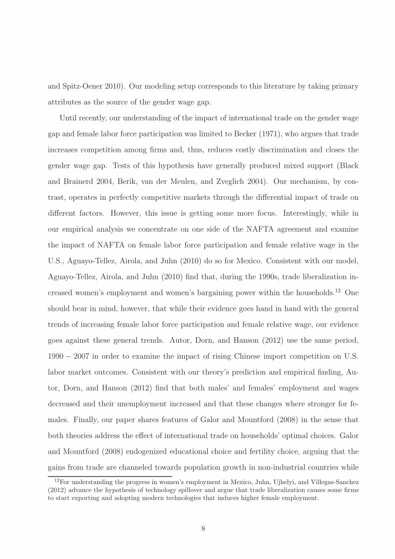
Equation (14) implies that in the case in which γ ≥ 1/2 women raise children full time

regardless of their wages. We rule out this scenario by imposing γ < 1/2. Under this

restriction, women raise children full-time only under relatively high gender wage gaps. But

as the gender gap decreases women join the labor force and fertility decreases. When wFt

approaches wMt , women spend a fraction 2γ of their time raising children. Finally, under our

assumption γ < 1/2 the budget constraint (4) collapses to

st = (1− znt)wFt + wM

t (15)

and (14) becomes with ωt = wMt /wF

t

znt = min {γ (1 + ωt) , 1} . (16)

2.4 Closed Economy

2.4.1 Static Equilibrium

The equilibrium of the integrated economy is determined separately for two regimes. The

first is a regime in which women do not participate in the formal labor market, and the

second is a regime in which women participate. To simplify the analysis, we assume that, in

equilibrium, the second sector is too small to accommodate all male labor. Specifically, we

assume17

2− α ≥ 1/θ (17)

to be satisfied throughout the following analysis. Under this assumption, Lp1,t > 0 holds and

the ratio of male to female wage can be computed by the marginal productivities in the first

17A sufficient condition for l1,t > 0 is that the relative price (7) falls short of the ratio of marginal rates of

transformation at l1,t = 0 and znt = 0 i.e. (1− α)καt a/b+ 1 > (1− θ) /θ (κα

t a/b)1−ρ. If κα

t a/b ≥ 1 then thissufficient condition is implied by (1− α) ≥ (1− θ) /θ, or (17). If κα

t a/b < 1 instead, the sufficient conditionis implied by 1 > (1− θ) /θ and hence, again, by (17).

14

sector

ωt = 1 +b

(1− α)aκαt

. (18)

This ratio determines female labor force participation 1− znt through (16)

znt = min

{

γ

(

2 +b

(1− α)aκαt

)

, 1

}

. (19)

To determine equilibrium κt, combine male wage (12), prices (7), and the resource constraint

for male labor 1 = l1,t + l2,t to get

(1− α)a

bκαt + 1 =

1− θ

θ

( abκαt mt + l1,t

1− l1,t

)1−ρ

. (20)

Further note that

l1,t = mt − (1− znt) (21)

so that equation (20) becomes

(1− α)a

bκαt + 1 =

1− θ

θ

( abκαt mt +mt − (1− znt)

1−mt + (1− znt)

)1−ρ

. (22)

Equations (6), (19), and (22) determine mt and znt and thus the equilibrium. There are two

qualitatively different types of equilibria to distinguish.

The First Regime znt = 1. In the case in which znt = 1, equation (22) can be written in

terms of κt (substitute mt = kt/κt):

(1− α)a

bκαt + 1 =

1− θ

θ

( ab

ktκ1−αt

+ ktκt

1− ktκt

)1−ρ

. (23)

15

The Second Regime znt < 1. In case in which znt < 1 we use mt = kt/κt and znt from

(19) to write (22) as

(1− α)a

bκαt + 1 =

1− θ

θ

ab

ktκ1−αt

+ ktκt

− 1 + γ(

2 + ba

κ−αt

1−α

)

1− ktκt

+ 1− γ(

2 + ba

κ−αt

1−α

)

1−ρ

. (24)

Equations (23) and (24) determine the equilibrium κt in the first and second regime, re-

spectively. Notice that expressions on the left of both equations are increasing in κt, while

both terms on the right are decreasing in κt. This implies that κt is unique in both regimes.

Moreover, the expressions on the right of (23) and (24) are increasing in kt so that κt(kt) is

an increasing function.

Quite intuitively, a capital-rich economy has a higher capital-mental labor share than a

capital-scarce economy. When going back to equation (19), this observation shows also that

the higher the capital stock kt of an economy, the lower fertility znt is. As κt(kt)|kt=0 = 0,

(19) further implies that there is a ko > 0 so that the economy is in the first regime when its

capital stock falls short of ko, while the economy is in the second regime if not. By combining

the according condition γ (2 + b/ [(1− α)aκαo ]) = 1 with equation (23) and κo = ko/mo, this

threshold is shown to be

ko = θ (1− γ)

(

1− 2γ + γ1− αθ

1− α

)

−1 [(1− α)(1− 2γ)

γ

a

b

]

−1/α

. (25)

At capital stocks below the threshold ko all women raise children full-time. When capital

is gradually accumulated and this threshold is passed, women integrate into the labor market

and, as the variable κt keeps increasing, the gender wage gap closes and female labor supply

rises. At the same time, and as a mirror image, fertility declines.

These observations regarding the impact of the capital stock on fertility and on female

labor force participation bring us to the dynamics of the model.

16

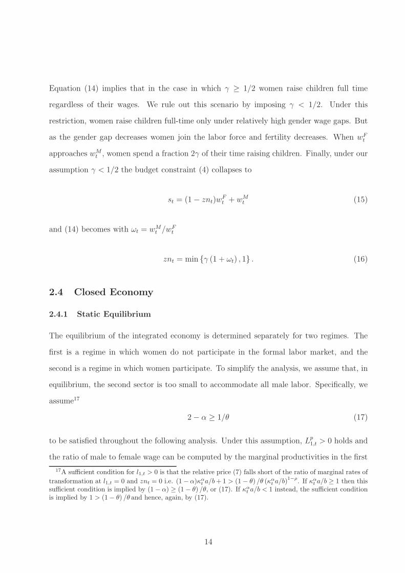
2.4.2 Dynamics

The dynamics of the model are governed by two endogenous variables: savings st and fertility

nt. With the notation in per-household terms, the ratio of saving and fertility gives the next

period’s capital stock, i.e. kt+1 = st/nt. Combining the budget constraint (15) and fertility

(16) and distinguishing the two regimes, we can write

kt+1 =stnt

=

zwMt if kt < ko

z 1−γγwF

t if kt ≥ ko.(26)

Recalling that πt =p2,tp1,t

, together with equations (10) and (11), leads to the following price

ratio

πt = (1− α)a

bκαt + 1 (27)

which, combined with the normalization (8), renders the price of the first intermediate good

p1,t =

(

θ1/(1−ρ) + (1− θ)1/(1−ρ)

(

1

(1− α)abκαt + 1

)ρ/(1−ρ))(1−ρ)/ρ

.

With (10) - (13) and (26) we thus have

kt+1 =

zb(

θ1

1−ρ

(

(1− α)abκαt + 1

)ρ

1−ρ + (1− θ)1

1−ρ

)1−ρρ

if kt < ko

zb1−γγ

(

θ1

1−ρ

(

(1− α)abκαt

)ρ

1−ρ + (1− θ)1

1−ρ

(

(1−α)abκαt

(1−α)abκαt +1

)ρ

1−ρ

)1−ρρ

if kt ≥ ko.

(28)

These expressions show that in both regimes, kt+1 is increasing in κt and thus, since κt is

an increasing function in kt, the schedule kt+1(kt) of the dynamic system is described by an

increasing function.

We can now make two observations, which jointly imply the existence of a steady state

under the second regime. First, the variable κt determined by (23) or (24) as well as the

threshold capital stock (25), are independent of z. Thus, given that z is sufficiently large,

17

an economy with per-household capital stock kt = ko from (25) experiences positive capital

growth due to capital accumulation (28): its capital stock in period t+1 exceeds its capital

stock of the previous period, i.e. kt+1 > kt holds. Second, as kt grows unbounded, the ratio

κt/kt = 1/mt is bounded from above.18 Thus, dividing the second line on the right hand side

of equation (28) by kt shows that kt+1/kt approaches zero as kt grows unbounded. Together,

these findings imply that, if z is sufficiently large, the dynamic system has a steady state in

the second regime.

Our knowledge about the dynamics and the steady state of the system is sufficient to

tell a simple story about economic development and female labor force participation. In an

economy where capital is scarce, female labor force participation is zero. As time passes and

per-household capital stock gradually accumulates, the rewards of formal employment for

female workers increase relative to rewards for male workers. This closing of the gender wage

gap fosters female labor force participation and curbs fertility. Both effects accelerate per-

household capital accumulation, which continues under the second regime up to the point

where the economy reaches its steady state.

Up to this point, our two-sector model essentially replicates the main features of the

model in Galor and Weil (1996). Rather than proving robustness of their results in a two-

sector setting, our intention is to analyze the impact of international trade and specialization.

We turn to this task next.

2.5 International Trade

We now turn to the effects of international trade in goods.19 As trade induces specialization

at the country level, countries expand some sectors while contracting others. As sectors

differ in intensity of male and female labor, international specialization affects relative wages

within each country. In the following paragraphs, we explore these effects of trade on the

18See Appendix.19We assume that capital is immobile, i.e. it is restricted to remain within national borders. This is partly

motivated by the strong home-bias of investment and, more importantly for our purpose, by the fact thatdifferences in the factor content of trade are consistent with the Heckscher-Ohlin predictions (Debaere 2003).

18

gender wage gap and the consequences for fertility and female labor force participation.

We assume that the world consists of two countries, Home (no ∗) and Foreign (∗). In

addition, the superscript A indicates autarky variables, while its absence indicates variables

of the free trade equilibrium. Moreover, we denote the relative population size of Foreign to

Home by λt = L∗

t/Lt.

Writing kt for the average per household capital stock of the world economy, we define

the set of all possible factor distributions in a world as:

FD t ={

(λt, kt, k∗

t ) | λt ∈ [0,∞]; kt, k∗

t ≥ 0 and (kt + λtk∗

t ) /(1 + λt) = kt}

, (29)

This definition comprises all possible partitions of the capital stock. Notice that the definition

depends on the world capital ratio kt but is independent of the world population size Lt+L∗

t .20

2.5.1 Factor Price Equalization

A good starting point for the analysis of the free trade equilibrium is the Factor Price

Equalization Set21

FPES t ={

(λt, kt, k∗

t ) ∈ FDt | wM = w∗,M , wF = w∗,F , r = r∗

}

. (30)

Among all possible distributions of factors across countries, the FPES t comprises those that

lead to free trade equilibria characterized by identical factor prices across countries. In terms

of prices and output, these equilibria then replicate the equilibrium of an integrated world

economy where factors are not restricted by national borders.22 Thus, the FPES t describes

the conditions on factor distributions under which borders do not affect the world efficiency

20The definition thus slightly deviates from the standard definition in the sense that it is formulated”modulo population size.”

21Remember that the absence of superscript A indicates equilibrium variables under free trade – e.g. atwM , w∗,M etc.

22If the equilibrium of the integrated economy is replicated, factors in all countries must equalize. Con-versely, if factor and good prices equalize in both countries, the world equilibrium is an equilibrium of theintegrated economy.

19

frontier. Loosely conceptualized, a factor allocation is an element of the FPES t if relative

factors are distributed “not too unevenly”.

The following proposition conveniently characterizes the FPES t of the present model.

Proposition 1

Factor prices equalize if and only if κ∗

t = κt.

Proof. See Appendix.

The proposition shows that κt = κ∗

t = κt implies ωt = ω∗

t , a regime in which fertility,

determined by (16), equalizes in both countries: znt = zn∗

t = znt.23 Combining these

equations leads to:

κt =kt

l1,t + 1− znt=

k∗

t

l∗1,t + 1− znt. (31)

By the definition of the FPES t, κt and nt are also the capital-mental labor ratio and fertility

of the integrated world economy.

For the rest of the analysis, and without loss of generality Home will represent the capital

scarce and Foreign the capital abundant country, i.e., we assume that kt < k∗

t for the initial

period. Making use of this inequlality in combination with (31), we observe that l1,t < l∗1,t

and thus l2,t > l∗2,t. Consequently, the relevant resource constraints l1,t, l∗

2,t ≤ 1 lead to a

restriction on capital stock conditions for factor price equalization to hold:

(1− znt)κt ≤ kt, k∗

t ≤ (2− znt)κt (32)

As capital stocks of both countries add up to the aggregate world capital stock (kt =

(kt + λtk∗

t ) /(1 + λt)), the FPES t is described by (32) and

λt =kt − ktk∗

t − kt. (33)

23Upper bars indicate variables of the integrated economy.

20

Using the concise graphical representation from Helpman and Krugman (1985), Figure 1

illustrates the FPES t. Each point A on the plane represents a partition of world labor and

world capital: the distance between the vertical axis and A represents Home’s male labor

Lt, while the distance between the horizontal axis and A represents Home’s capital Kt;

Foreign’s variables are L∗

t = Lt − Lt and K∗

t = Kt − Kt, respectively. Since female labor

shares are determined by the gender wage gap and hence by factor prices only, factor price

equalization implies that female labor shares equalize in both countries. Thus, in the case

where global female labor shares are positive, Home must hold a minimum level of capital

to keep X1-production operating and generate jobs in this sector. This case is illustrated in

the top panel of Figure 1. If, instead, global female labor shares are zero, Home may in fact

entirely lack capital. By fully specializing on X2-production, Home’s factor prices may still

equalize with Foreign’s. In this case, which is illustrated by the bottom panel of Figure 1,

the equilibrium of the integrated economy is replicated.

We can now readily determine the specialization pattern of both economies under the

assumption that factor prices equalize. Recalling assumption kt < k∗

t , we observe:

mt = kt/κt < k∗

t /κt = m∗

t ,

while

l2,t = 1− [mt − (1− znt)] > 1− [m∗

t − (1− znt)] = l∗2,t.

Confirming Heckscher-Ohlin-based intuition, the capital scarce Home country specializes in

production of the labor intensive good, X2, while capital abundant Foreign specializes in

X1-production.

We can further compare the trade equilibrium with the respective autarky equilibria. To

do so, we use κAt < κt < κ∗,A

t and (19) to conclude:

znAt ≥ znt ≥ zn∗,A

t .

21

These inequalities are strict if 1 > znAt holds. Consequently, relative to autarky, trade

increases female labor force participation in the capital scarce country and decreases it in

the capital abundant country.

These observations combined imply that the country which, by international special-

ization, contracts the sector that is particularly suitable for female labor, experiences an

increase in female labor force participation. Conversely, the country which expands the

sector suitable for female labor, experiences a decrease in female labor force participation.

The reason for this seemingly paradoxical finding is the following. For each economy, the

key determinant of female labor force participation is the gender wage gap ω(∗)t . In autarky

and under factor price equalization, this gender wage gap is determined by the relative

productivities in the X1-sector via (18) and ultimately by the capital-mental labor ratio κ(∗)t .

When international specialization induces Home to contract its X1-sector and expand its X2-

sector, male workers move from the first to the second sector, taking their mental labor with

them. Thus, they increase the ratio κt and thereby foster female labor force participation

(1− znt). Conversely, when Foreign workers react to trade-induced international price shifts

and move from the second to the first sector, they dilute the capital-mental labor share κ∗

t ,

which increases the gender wage gap and decreases female labor force participation.24

In sum, under factor price equalization, we get sharp results on the impact of trade on

female labor force participation in the capital scarce and abundant countries, respectively.

The key mechanism for the result described above, however, depends on the fact that the

gender wage gap is a function of the capital-mental labor ratio κ(∗)t . The extent to which

these results generalize beyond factor price equalization is the subject of the next subsection.

24The effect of relative productivities on the gender wage gap, which is the core of our mechanism operatesunder substantial generalizations. If F (K,M,L) represents a standard constant return to scale productionfunction in the first sector, it is sufficient to assume that capital K complements mental labor M relativelymore than physical labor L (i.e. , FKM/FM > FKL/FL ≥ 0, in line with Goldin (1990) and Galor andWeil (1996)) in order to generate the effect discussed. In particular, under these conditions, higher maleemployment in the first sector increases the gender wage gap (Saure and Zoabi 2011).

22

2.5.2 Beyond Factor Price Equalization

Let us begin the general case of international trade by focusing on one country, for example,

Home, with exogenous relative world prices πt – i.e., for the moment, we assume that Home

is a small open economy. We determine how the equilibrium gender wage gap ωt changes

with world price πt = p2,t/p1,t. This is done in the following Lemma.

Lemma 1

(i) For given capital endowment kt there are π, π with 0 < π < πAt < π so that

d

dπt

ωt(πt) =

0 if πt ≤ π

< 0 if πt ∈ (π, π)

> 0 if πt ≥ π

(ii) Output of the X1- (X2-) sector is weakly decreasing (increasing) in πt.

Proof. (i) At autarky price πAt , we have l1,t, l2,t > 0, as shown in the closed economy.

Combining (10), (11), and (13) we have πt = (1− α) a/bκαt +1 and ωt = πt[(1− α) a/bκα

t ]−1

and hence

ωt =πt

πt − 1(34)

as long as l1,t, l2,t > 0, implying that ωt is decreasing in πt. By (16) this means that znt is

decreasing in πt, in this range too. Further, πt = (1− α) a/bκαt + 1 implies that κt = kt/mt

is increasing in πt and hence, as mt = l1,t + 1 − znt, must be decreasing in πt. Therefore,

l1,t(πt) is decreasing in πt. The constraint l1,t ∈ [0, 1] then implies that there are two prices

π and π so that l1,t(π) = 1 and l1,t(π) = 0. Consider now prices πt with πt ≤ π and check

that (12) gives

ωt = 1 + [(1− α) a/bκαt ]

−1 (35)

23

Thus, ωt is constant in πt (check with (10) and (11) that l1,t = 1 throughout this range). For

prices πt satisfying πt ≥ π (12) implies

ωt = πt[(1− α) a/bκαt ]

−1 (36)

Thus, starting at πt = π, increases in πt cannot increase mt = 1− znt ((16) would require a

decrease in ωt contradicting equation (36)) and must widen the gender wage gap ωt. Check

with (10) and (11) that l1,t = 0 throughout this range.

(ii) Output of X2 is proportional to 1 − l1,t and l1,t has been shown to be decreasing

in (i). – Consider output of X1. In the range πt < π, l1,t = 1 and ωt constant. Hence,

mt = l1,t + 1 − znt is constant and so is output of X1. In the range πt ∈ (π, π) the gender

wage gap ωt is decreasing and hence κt increases, as (18) holds. Thus, X1 from (2) decreases.

Finally, for πt > π the employment mt = 1 − znt in X1-sector decreases (ωt increases while

l1,t = 0 holds). Thus, X1 output falls.

Figure 2 summarizes part (i) of the Lemma. For small πt, the gender wage gap ωt (πt) is

constant: all factors are employed in the first sector and small price changes do not change the

labor allocation, so that relative factor rewards are constant. Conversely, for πt > π, all male

workers are employed in the second sector, while capital and female labor are employed in

the first sector. Again, small price changes do not change the labor allocation, but translate

one-to-one into changes in the wage gap. Finally, for the intermediate range πt ∈ (π, π),

the gender wage gap ωt (πt) is decreasing through the effects of labor allocation explained

already in the case of factor price equalization. By the generic relation (16), these swings in

ωt are paralleled by swings in znt.

Part (ii) of the Lemma simply states the basic scheme of international trade: as import

prices drop, an economy increases its import volume and shifts production towards its export

sector.

24

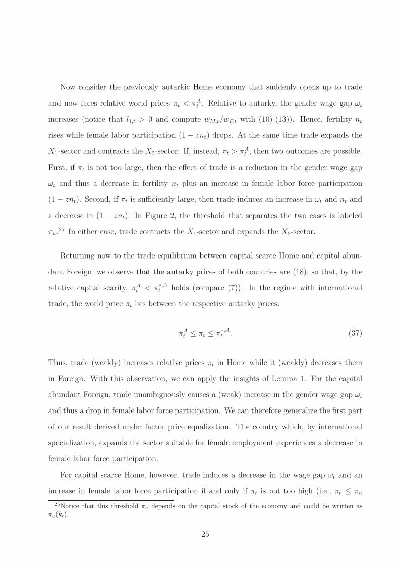
Now consider the previously autarkic Home economy that suddenly opens up to trade

and now faces relative world prices πt < πAt . Relative to autarky, the gender wage gap ωt

increases (notice that l1,t > 0 and compute wM,t/wF,t with (10)-(13)). Hence, fertility nt

rises while female labor participation (1− znt) drops. At the same time trade expands the

X1-sector and contracts the X2-sector. If, instead, πt > πAt , then two outcomes are possible.

First, if πt is not too large, then the effect of trade is a reduction in the gender wage gap

ωt and thus a decrease in fertility nt plus an increase in female labor force participation

(1− znt). Second, if πt is sufficiently large, then trade induces an increase in ωt and nt and

a decrease in (1 − znt). In Figure 2, the threshold that separates the two cases is labeled

πu.25 In either case, trade contracts the X1-sector and expands the X2-sector.

Returning now to the trade equilibrium between capital scarce Home and capital abun-

dant Foreign, we observe that the autarky prices of both countries are (18), so that, by the

relative capital scarity, πAt < π∗,A

t holds (compare (7)). In the regime with international

trade, the world price πt lies between the respective autarky prices:

πAt ≤ πt ≤ π∗,A

t . (37)

Thus, trade (weakly) increases relative prices πt in Home while it (weakly) decreases them

in Foreign. With this observation, we can apply the insights of Lemma 1. For the capital

abundant Foreign, trade unambiguously causes a (weak) increase in the gender wage gap ωt

and thus a drop in female labor force participation. We can therefore generalize the first part

of our result derived under factor price equalization. The country which, by international

specialization, expands the sector suitable for female employment experiences a decrease in

female labor force participation.

For capital scarce Home, however, trade induces a decrease in the wage gap ωt and an

increase in female labor force participation if and only if πt is not too high (i.e., πt ≤ πu

25Notice that this threshold πu depends on the capital stock of the economy and could be written asπu(kt).

25

holds).26 In this restricted case, we recover the second part of the result derived under

factor price equalization. The country which contracts the sector suitable for female labor

experiences an increase in female labor force participation. This second observation is a

non-trivial generalization of the parallel result under factor price equalization. To verify this

statement, use that under free trade l∗1,t > 0 and l2,t > 0 hold so that, by (10) and (11)

(1− α)a

b(κ∗

t )α + 1 ≥ πt ≥ (1− α)

a

bκαt + 1 (38)

holds. Proposition 1, however, states that factor price equalization requires κt = κ∗

t , implying

πt = (1− α) abκαt +1. By construction of π, however, all world equilibria with πt ∈ (π, πu) are

characterized by equality πt > (1− α) abκαt + 1, implying that factor prices do not equalize.

Since finally, by construction of πu we have ωt > ωAt for all equilibria with πt ∈ (π, πu) we

conclude that trade induces an increase of female labor force participation in Home for a set

of factor endowments that is strictly larger than the FPESt.

Summarizing, we use the definitions (29) and (30) to state the following proposition.

Proposition 2

(i) In Foreign, trade expands the sector that uses female labor intensively, but unambigu-

ously reduces female labor force participation.

(ii) There is a set St ⊂FDt with FPESt $ St and the following property: for each element

of St trade contracts the sector that uses female labor intensively in Home, but increases

Home’s female labor force participation.

It is important to stress that this general result does not rely on the close link between

female labor force participation and fertility. Instead any time-intensive home production

will render the very same result.

Notice that, by virtue of the previous Lemma, the first statement of the proposition also

holds at the margin. Any marginal trade liberalization in the capital rich country that lowers

26Notice that, by assumption (17) π∗,At < πu holds for Foreign. However, the threshold πu(k

∗

t ) depends

on Foreign’s capital and one cannot conclude that πt ≤ π∗,At < πu(kt) holds.

26

the relative import over export price widens the gender wage gap and hence decreases female

labor force participation.

2.5.3 Dynamics under Trade

We now turn to the dynamics of the model under free trade. Again, these are driven by

two key variables, savings st and fertility nt. Per-household capital stocks of either country

follow the generic dynamic system equivalent to (26), now expanded to:

k(∗)t+1 =

zwM,(∗)t if zn

(∗)t = 1

z 1−γγw

F,(∗)t if zn

(∗)t < 1

(39)

To calculate the respective wages, we can use the final good normalization (8) and the

definition of πt to derive:

p1,t =

(

θ1

1−ρ + (1− θ)1

1−ρ π−ρ1−ρ

t

)(1−ρ)/ρ

and p2,t =(

θ1

1−ρπρ

1−ρ

t + (1− θ)1

1−ρ

)(1−ρ)/ρ

(40)

With these expressions, together with the definition of wages (10) - (13) and the dynamic

system (39), we can shoe the following statements

Proposition 3

(i) zn∗

t ≤ znt.

(ii) k∗

t+1 ≥ kt+1.

(iii) If α(θ/(1− θ))1

ρ−1 ≥ (1− 2γ) /γ holds then kt+1 ≥ kAt+1.

(iv) k∗

t+1/kt+1 ≤ k∗,At+1/k

At+1.

Proof. See Appendix.

Parts (i) and (ii) of the proposition show that trade cannot reverse the order of countries

regarding population growth or capital abundance. Relative to the poor country, the capital

rich country has always weakly lower fertility rates, higher female labor force participation

and a higher per-household capital stock.

27

Proposition 3 (iii) shows that, if the first sector is sufficiently large (i.e., 1−θ is sufficiently

small), trade unambiguously accelerates the pace of capital accumulation in the capital

scarce country. It is worth emphasizing that this result also holds in the case where world

prices πt are very large and all men in Home work in the X2-sector while female labor

participation drops relative to autarky (πt > πu in Figure 2). Even in this case, where a

reduced female labor force participation depresses savings and increased population growth

dilutes the following period’s per household capital stock, the gains from trade are sufficient

to grant a net increase in per-household capital accumulation relative to autarky. We cannot,

however, make a parallel statement for the capital rich economy, for which the effect of trade

on capital accumulation is ambiguous. Indeed, it can be shown that for capital accumulation

in the rich economy, the positive forces stemming from the gains of trade might either

dominate or be dominated by the adverse effect of reduced female labor force participation

and higher fertility.

In sum, Proposition 3, shows that in transition to an economy’s steady state, international

trade fosters convergence in fertility, labor force participation, and per-household capital

stocks. Notice, that we do not make any statements characterizing the steady states of the

two economies. The reason for this restraint is that the steady state is not necessarily unique

in our model. Therefore, there may be discrete long-run effects of trade on income and female

labor force participation. A possible scenario is the following. A the poor economy trapped in

a steady state with a low capital stock, low female labor force participation and high fertility

(compare Galor and Weil (1996)). When this economy opens up to trade with a capital rich

economy, the arising gains from trade and the reduced fertility rates lift this economy up,

which consequentially escapes from the poverty trap by trading. In this case, international

trade takes the role that Galor and Weil (1996) attriute to technological progress. Indeed,

technological progress helps to eliminate poverty traps in the case of closed economies. We

will briefly turn to this scenario next.

28

2.6 Technological Progress

The reduction in the gender wage gap is sometimes attributed to technological change.

Welch (2000), Gosling (2003) and Black and Spitz-Oener (2010) argue that the increase in

the market price for women’s labor was brought about by a relative increase in the valuation

of skill (mental labor endowments), which is, at least in part, explained by technological

change. Galor and Weil (1996) show how technological change can eliminate poverty traps,

characterized by high fertility, low female labor force participation and low per-household

capital stocks. They argue that “technological progress will eventually eliminate such a

development trap, leading to a period of rapid output growth and a rapid fertility transition”

(p. 383).

Another popular hypothesis rests on demand shifts in favor of goods whose production

is more intensive in skill or, more generally, in female labor inputs. The mechanism outlined

above, in which male workers searching for the highest return to their labor crowd out women

in the labor market sheds some doubt on the generality of these pro-growth effects. Indeed,

we show next that the effect that leads to a decrease in female labor force participation and

an increase in fertility in response to the expansion of the females’ comparative advantage

sector operates under technological change and shifts in demand as well.

For the formal analysis of technological change and demand shifts, we return to the closed

economy. To incorporate technological change biased towards the sectors that generate

demand for female labor, we rewrite the production functions (2) as:

X1 = µ[

aKαt (L

mt )

1−α + bLp1,t

]

X2 = bLp2,t

(41)

so that growth of the parameter µ ≥ 1 mimics technological progress that is biased towards

29

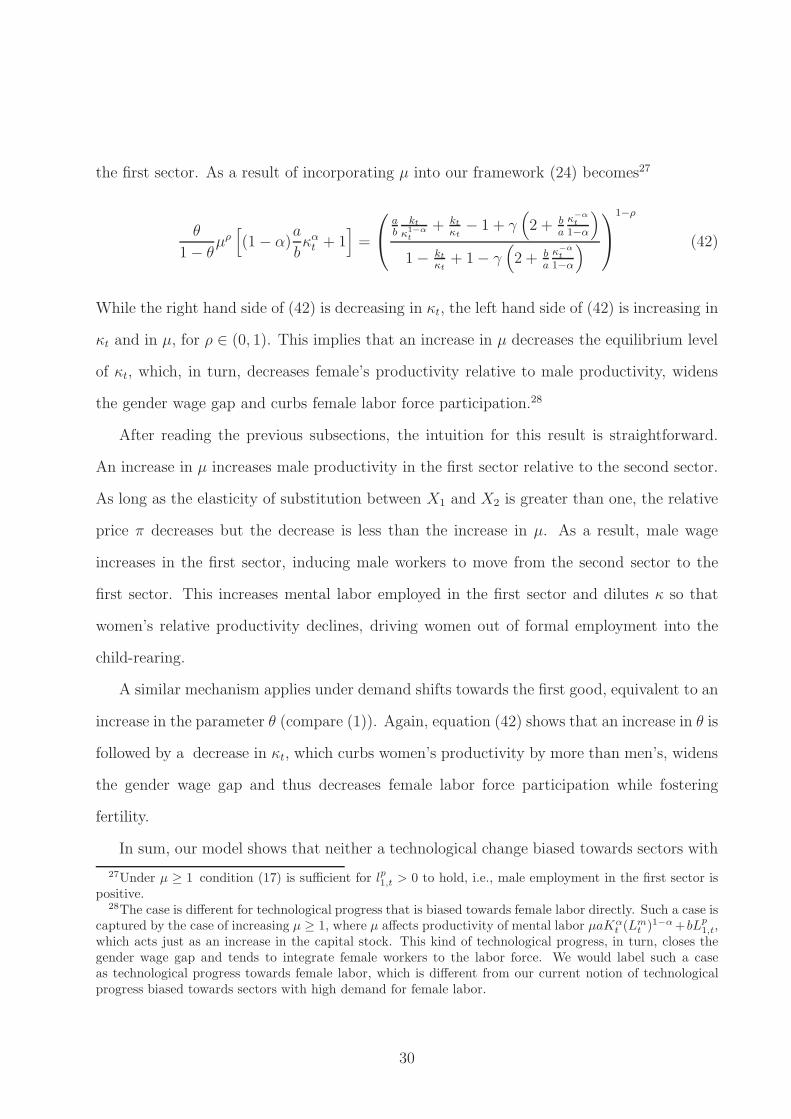
the first sector. As a result of incorporating µ into our framework (24) becomes27

θ

1− θµρ[

(1− α)a

bκαt + 1

]

=

ab

ktκ1−αt

+ ktκt

− 1 + γ(

2 + ba

κ−αt

1−α

)

1− ktκt

+ 1− γ(

2 + ba

κ−αt

1−α

)

1−ρ

(42)

While the right hand side of (42) is decreasing in κt, the left hand side of (42) is increasing in

κt and in µ, for ρ ∈ (0, 1). This implies that an increase in µ decreases the equilibrium level

of κt, which, in turn, decreases female’s productivity relative to male productivity, widens

the gender wage gap and curbs female labor force participation.28

After reading the previous subsections, the intuition for this result is straightforward.

An increase in µ increases male productivity in the first sector relative to the second sector.

As long as the elasticity of substitution between X1 and X2 is greater than one, the relative

price π decreases but the decrease is less than the increase in µ. As a result, male wage

increases in the first sector, inducing male workers to move from the second sector to the

first sector. This increases mental labor employed in the first sector and dilutes κ so that

women’s relative productivity declines, driving women out of formal employment into the

child-rearing.

A similar mechanism applies under demand shifts towards the first good, equivalent to an

increase in the parameter θ (compare (1)). Again, equation (42) shows that an increase in θ is

followed by a decrease in κt, which curbs women’s productivity by more than men’s, widens

the gender wage gap and thus decreases female labor force participation while fostering

fertility.

In sum, our model shows that neither a technological change biased towards sectors with

27Under µ ≥ 1 condition (17) is sufficient for lp1,t > 0 to hold, i.e., male employment in the first sector is

positive.28The case is different for technological progress that is biased towards female labor directly. Such a case is

captured by the case of increasing µ ≥ 1, where µ affects productivity of mental labor µaKαt (L

mt )1−α+bLp

1,t,which acts just as an increase in the capital stock. This kind of technological progress, in turn, closes thegender wage gap and tends to integrate female workers to the labor force. We would label such a caseas technological progress towards female labor, which is different from our current notion of technologicalprogress biased towards sectors with high demand for female labor.

30

high demand for female labor nor demand shift towards goods of these sectors necessarily

generates increases in female labor participation. The resulting increase in fertility generally

counters the pro-growth effects.

3 Empirical Evidence

Our theory predicts that, when trading with a poor economy, trade decreases aggregate

female labor force participation and female relative wage in the rich economy. We choose to

test the predictions through the surge in U.S.-Mexican trade during the period 1990–2007, a

period of trade liberalization, which we simply label the “NAFTA episode” in the following.29

A brief explanation of our empirical strategy seems appropriate. One may argue that

focusing on aggregate female labor is not the most direct way to test our theory but rather

examining the reallocations of male and female labor across sectors. However, two crucial

reasons dictate our choice. First, the empirical trade literature found that industry-level

data hide substantial intra-industry product heterogeneity (Schott 2003). Moreover, Schott

(2004) reports that capital-abundant economies use their endowment advantage to produce

vertically different varieties. Finally, Bernard, Jensen, and Schott (2006) documents that,

as industry exposure to imports from low-wage countries rises, labor in U.S. manufacturing

reallocates away from labor-intensive plants and toward capital-intensive plants within in-

dustries. Overall, our theory may affect labor reallocation at the intra-industry level: either

across vertically superior varieties or across plants with different capital intensities so that

industry level data reveals only part of the trade-induced labor reallocation. Second, and as

we explain in the introduction, aggregate female labor drops in response to trade liberaliza-

tion, while female employment in the female intensive sector may stay constant or actually

increase.

29This label is misleading to the extent that not all of the increase in US-Mexican trade is attributed totariff reductions of NAFTA. In fact, Krueger (1999) argues that Mexico’s unilateral tariff reduction in thelate 1980s and its abandoning of the exchange rate peg explains most of the increase in trade volumes. Forthe purpose of our test, however, this observation is of minor importance. We are only concerned aboutidentifying an episode of substantial increase in trade volumes.

31

The choice of the NAFTA episode has a number of virtues. First, the U.S. and Mexico

are paradigmatic for a pair of capital-rich and capital-poor economies, for which our theory

applies.30 As a second advantage of the NAFTA episode, U.S.-Mexican trade experienced

a substantial growth during that period: U.S. trade with Mexico as a share of U.S. GDP

increased more than three-fold between 1990 and 2007, while Mexico’s share in U.S. total

trade rose by a factor of more than two (Figure 3). Via this substantial increase of bilateral

trade volumes, we hope to identify a sizable impact of trade on labor markets. Third, the

choice of the NAFTA episode allows us to take advantage of the high quality of U.S. trade

and labor market data. In particular, we can exploit exposure to trade with Mexico on

a U.S. state level. Finally, due to the specific geographical constellation, U.S. trade with

Mexico is particularly uneven across U.S. states, which allows us to use distance as a powerful

instrument for a change in trade volumes and thus establish causality running from change

in trade to change in female labor share and female relative wage.

In deciding whether to emphasize wages or employment in our empirical analysis, we

notice that the empirical trade literature has documented an asymmetric impact of glob-

alization on employment and wages. In particular, liberalization of goods markets appears

to have a sizable effect on employment but a rather small effect on wages (Grossman 1987,

Revenga 1992). This asymmetry may be a result of labor reallocation itself, which tends to

erase wage differentials and mitigate wage effects. Alternatively, a selection bias problem

blurs the impact of trade on wages as workers with specific characteristics systematically

exit the labor market Therefore, our empirical part stresses the impact of exogenous change

in trade on female labor force participation. However, to complete the picture, we also test

for its impact on female relative wage.

30Capital stocks per worker can be calculated from real investment data as in PWT6.2. At depreciationrates of between .01 and .1, the relative capital stock of the U.S. in 2003 exceeded that of Mexico by a factorof four. Consistent with our theory, the female labor share in the U.S. ranged from 43.1 to 46.3 between1985 and 2006, while the according range for Mexico is 29.4 to 35.3 (United Nations Statistics Division).

32

3.1 Data

We rely on three different data sources. First, we use is the March Current Population Survey

conducted by the Integrated Public Use Microdata Series (IPUMS-CPS).31 From IPUMS-

CPS we take the variables age, sex, marital status, population status (to distinguish between

civilian or Armed Forces), nativity (to identify immigrants), location (state), Hispanic origin

(to identify Mexicans), educational attainment, employment status (to compute the formal

employment share) weeks worked, usual hours worked (to compute total hours worked) and

wage and salary income (to compute hourly wage). Table 2 provides descriptive statistics for

female and male labor for the years 1990/91 and 2006/07. Two observations can be drawn

from Table 2 during the NAFTA episode: first, while female labor force participation has

increased, male labor force participation has decreased and, second, the hourly wage for both

genders has increased during the same period. The second database we use is the ‘Origin

of Movement’ administered by WISER,32 which covers export data by state and destination

country from 1988 onward. These data are disaggregated by goods categories (SIC from

1988 to 2000; NAICS from 1997 onward). Third, we use the Bureau of Economic Analysis

for GDP data on the state level.33

3.2 Female labor force participation

3.2.1 The Empirical Model

In our empirical exercise, we concentrate on one side of our theory and aim to identify the

effect of trade on the U.S. labor market (the capital rich economy). More precisely, we exploit

the variation of U.S.-Mexican trade across different U.S. states to identify the differential

impact of trade on female labor shares and female relative wage across states.34

31King, Ruggles, Alexander, Flood, Genadek, Schroeder, Trampe, and Vick (2010).32World Institute for Strategic Economic Research; data available under http://www.wisertrade.org.

Cassey (2009) gives a good introduction to the data and their limitations.33Data available under http: http://bea.doc.gov/regional/.34The focus on U.S. states as economic entities may seem problematic since state borders are not relevant

restrictions for the labor. This drawback, however, implies that inter-state labor migration can eliminate

33

As discussed in the introduction, previous empirical literature has revealed that the

impact of trade liberalization on wages is smaller than the impact on employment and that

the latter is of marginal magnitude. Thus, we begin by examining whether NAFTA had any

impact on female employment at all, and subsequently move our attention to its impact on

wages.

According to our theory, a higher exposure to trade with Mexico induces lower female

labor force participation in the different U.S. states. Put differently, our theory suggests that,

other things equal, a state that is exposed to a larger expansion in trade will experience a

higher reduction in female labor force participation.

Analyzing this relation on the state level, our reduced form model takes the following

form:

∆ys = α + β∆Trades +X ′

sγ + us (43)

where for any variable, zs the s indicates the different U.S. states and ∆ indicates the change

over time - before and after NAFTA. The dependent variable ys is the female labor share,

Trades is trade volume per output. We control for a vector of covariates X ′

s chosen by

economic intuition but unrelated to our theoretical model. Our initial period is 1990-1,

while the end period is 2006-7.35 Our theory predicts that the estimate of β in (43) is

negative.

We first run an OLS regression of the type described in (43). However, labor market

conditions in the U.S., reflected by higher shares of female labor, can constitute a form

of comparative advantage and thus drive trade volumes. This edogeneity biases our OLS

estimates and leaves us with the need to instrument so as to establish the desired causality.

differences in the gender wage gap and female labor force participation across states, which tends to eliminatethe differential effects of trade across states. Thus, no differential effect of trade on female labor shares acrossstates can be expected as long as the U.S. labor market operates frictionless. Nevertheless, we expect tocapture labor market effects to the extent that frictions of labor movement related to geographical distanceimpede a full equalization of factor prices across U.S. states.

35This time window is determined by availability of trade data. The data set includes entries for the years1988/89 but these are of inferior quality.

34

We slightly modify the gravity equation of the trade literature and instrument ∆Trades

by distance to Mexico.36 Thus, our first stage regression is:

∆Trades = µ+ θ ds +X ′

s ρ+ νs (44)

where ds is distance of state s to Mexico.

Figure 4 illustrates that distance is strongly correlated with the increase in trade share,

thereby satisfying a first necessary condition for being a valid instrument.

Perhaps our instrument distance to Mexico has a direct effect on female labor force

participation or is correlated with other relevant variables that have an effect on female

labor force participation. Possible examples include development, culture or religiosity, which

typically correlate with latitude. However, by taking first difference we eliminate the state-

fixed effect. It still may be the case that distance is correlated with pace at which female

labor force participation changes. To verify this point, we perform the following additional

falsification test. Using data from the pre-NAFTA period, we regress a reduced form model

of the change in female labor force participation on distance. We find supportive evidence

for our presumption that only during the NAFTA period does distance positively impact the

change in female labor force participation, which suggests that the exclusion restriction is

likely to hold.37 One may still argue that during the NAFTA period changes in female labor

force participation were more prominent than during the pre-NAFTA period. As a result, we

observe the correlation between distance and changes in female labor force participation only

during the NAFTA period. Our presumption here is that culture and religiosity have not

changed during the period 1960–2000 and therefore if these characteristics were to impact the

correlation between distance and the pace at which female labor force participation changes

during the 90s, there is no reason to think that these same characteristics had no such impact

36More precisely, we regress trade volume as a percentage of Gross State Product on spherical distance ofU.S. state capitals to Mexico City, while the standard gravity equation estimates the log of bilateral tradevolume on the log of GDP, spherical distance and other variables.

37Exact details about our falsification test are explained in the First Appendix and its results are reportedin Table 8.

35

during the 60s. Moreover, looking at average female employment, it has increased during the

pre-NAFTA period by about 20 percent (from 31.2 percent in 1960 to 37.4 percent in 1970)

while it has increased during the NAFTA period by about 17 percent (from 54.4 percent in

1990 to 63.4 percent in 2000). This implies that the pace of change during the whole period

was more or less the same.

3.2.2 Control Variables

To control for differential business cycle effects across states, we include the change in log

per capita “Gross State Product” (GSP) and unemployment rate. We also control for the

change in average education level for females, which is positively correlated with female

labor share.38 Further, we include the share of Mexican immigrants, which might either

depress female labor participation – e.g. if cultural differences reduce gender labor market

participation39 – or else increase female labor participation – e.g. by increasing supply of

nannies and private child-care. We have no strong prior on the sign of this latter control

variable.

The secular trend towards higher female labor force participation together with the fact

that it is naturally bounded from above implies that female labor force participation con-

verges across states. Hence, the initial level of female labor share is highly correlated with

the change in female labor force participation. To account for this convergence effect, we

include the initial level of female labor force participation in the controls when estimating

(43). A problem with this control variable, however, is that it is correlated with the error

term in (43), wherefore we instrument it with lagged female labor participation (values from

1980/81). In choosing our instrument for the initial levels of female labor force partici-

38We define two categories of education. First, educated individuals who have at least some college-trainingand for whom we assign a weight of 1. Second, uneducated individuals who are at most high school graduatesand for whom we assign a weight of 0. The education level of a state is defined as the average of individualweights.

39On a national level, this concern seems unsubstantiated: national averages of female hours worked aspercentage of male hours worked of Mexicans exceed the according numbers of the full sample by 0.5% to1.9% between 1990 and 2007.

36

pation we thus assume that the levels in 1980/81 affect the changes in female labor force

participation during the period 1990/91–2006/7 only through the levels of 1990/91.

3.2.3 Regression Results

For our baseline specification, we define female labor participation as the share of hours

worked by females. Taking this share is not a strict necessity, but it eliminates labor market

shocks that are common to both sexes. In all our specifications, labor force is defined as the

total of individuals aged between 16 and 65, excluding members of the Armed Forces. We

further define exposure to trade as twice the state exports to Mexico over GSP. We restrict

the study to export because import data per state are not available.40 Distance is defined

as spherical distance from state capitals to Mexico City.

Table 3 reports the results of our baseline regression. Column 1 reports a simple OLS

regression of our dependent variable: change in female labor share on an initial level of

female labor share, which we take to be the average of 1980 and 1981 and the change in

trade with Mexico. As discussed earlier, we are not surprised by insignificant coefficient

of our main variable, ∆Trade with Mexico, since this OLS regression suffers from a bias

due to endogeneity problems. E.g. higher female labor force participation strengthens the

comparative advantage in the capital-intensive sector, which generates higher international

specialization and trade.

To avoid this endogeneity and to identify the causal relation running from change in

trade to female labor shares, we focus on the remaining five columns that summarize IV

estimates, where the change in trade is instrumented by distance. Column 2 reports estimates

without controls, Column 3 includes average female labor share of 1990 and 1991, which is

instrumented by the average values of 1980 and 1981; Column 4 includes the differences

of log per capita GSP and unemployment share; Column 5 includes differences in female

education share and Column 6 includes change in Mexican immigration share.

40We assume that import equalizes export in order to reveal, quantitatively, a more realistic coefficient oftrade on female labor share.

37

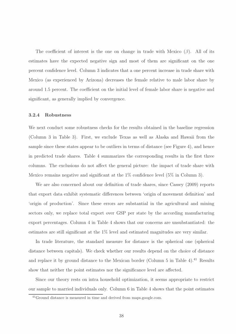
The coefficient of interest is the one on change in trade with Mexico (β). All of its

estimates have the expected negative sign and most of them are significant on the one

percent confidence level. Column 3 indicates that a one percent increase in trade share with

Mexico (as experienced by Arizona) decreases the female relative to male labor share by

around 1.5 percent. The coefficient on the initial level of female labor share is negative and

significant, as generally implied by convergence.

3.2.4 Robustness

We next conduct some robustness checks for the results obtained in the baseline regression

(Column 3 in Table 3). First, we exclude Texas as well as Alaska and Hawaii from the

sample since these states appear to be outliers in terms of distance (see Figure 4), and hence

in predicted trade shares. Table 4 summarizes the corresponding results in the first three

columns. The exclusions do not affect the general picture: the impact of trade share with

Mexico remains negative and significant at the 1% confidence level (5% in Column 3).

We are also concerned about our definition of trade shares, since Cassey (2009) reports

that export data exhibit systematic differences between ‘origin of movement definition’ and

‘origin of production’. Since these errors are substantial in the agricultural and mining

sectors only, we replace total export over GSP per state by the according manufacturing

export percentages. Column 4 in Table 4 shows that our concerns are unsubstantiated: the

estimates are still significant at the 1% level and estimated magnitudes are very similar.

In trade literature, the standard measure for distance is the spherical one (spherical

distance between capitals). We check whether our results depend on the choice of distance

and replace it by ground distance to the Mexican border (Column 5 in Table 4).41 Results

show that neither the point estimates nor the significance level are affected.

Since our theory rests on intra household optimization, it seems appropriate to restrict

our sample to married individuals only. Column 6 in Table 4 shows that the point estimates

41Ground distance is measured in time and derived from maps.google.com.

38

remain in the same range and only the significance level drops slightly to 5%.

Next, we replace the definition of our dependent variable from share of hours to relative

employment. This obviously eliminates the important intensive margin of individuals’ labor

market participation. Nevertheless, Column 7 in Table 4 shows that the estimates are

significant at the 5% level.

Our theory suggests that trade-induced specialization reduces female labor force par-

ticipation in capital-rich country while making male workers merely change sectors. Conse-

quently, we need to check that our results above are driven by changes in female employment

only. We do so by investigating the impact of trade on female and male working hours sepa-

rately. Average female hours per week were 22.77 (standard deviation across states is 1.92)

in 1990/1991 and 24.24 (1.84) in 2006/2007. The according numbers for male are 32.92

(1.89) and 32.2 (1.81), respectively (Table 2). These regressions are summarized in Table

5.42 While all point estimates of the coefficient on change in trade share with Mexico are

negative and significant for females, trade, overall, does not significantly impact male labor

hours: estimates are mostly insignificant, positive and around zero.

Finally, we limit our sample to highly educated individuals for several reasons. First,

our theory suggests that female labor force participation drops due to the decrease in the

relative price of mental labor, which may be associated with higher education. Second,

this limitation eliminates the possibility that our estimated effects stem from alternative

mechanisms.43 Consistent with our theory, Table 6 shows that all regressions exhibit a

negative impact of trade on female labor force participation, while such an impact does not

prevail for male workers.

42Columns 2, 4, 6 and 8 in Table 5 show that using population weight to unravel the impact of change intrade at the individual level does not change neither the magnitudes of our estimates nor their significance.

43Thus, one may conjecture that the estimates pick up a negative correlation between the share of unskilledwomen and distance from Mexico. In this case, in states neighboring Mexico, a larger share of women wouldbe affected by adverse wage shocks due to trade, resulting in a larger drop in female labor force participation.

39

3.3 Female Relative Wage

3.3.1 The Empirical Model

Since our mechanism suggests that trade and specialization affect female labor force partic-

ipation through females’ relative wages, we would like to empirically examine whether U.S.

trade with Mexico had the expected impact on the relative wages of U.S. females. Although

consensus exists in the literature that the impact of trade on wages is very weak we seek

to investigate whether higher trade with Mexico has an impact on the relative wage of U.S.

females and whether this impact has the expected sign.

According to our theory, a higher exposure to trade with Mexico induces lower female

relative wage in the different U.S. states. Put differently, our theory suggests that, other

things equal, a state that is subject to higher expansion in trade with Mexico will experience

a larger decreases in female relative wage.

Following the specification in (43), we analyze the relative wage on the state level with

the following empirical model

∆

(

wf

wm

)

s

= α′ + β ′∆Trades +X ′

sγ′ + vs (45)

The dependent variable ∆( wf

wm )s is the change in the relative wage of females in state s. We

keep the same notation of section 3.2. Our theory predicts that the estimate of β ′ in (45) is

negative.

We focus on one specification, which corresponds to the one in Column 3 of Table 3.

Accordingly, our first stage regression is the same as in (44). We control for the initial

level of relative wage, and in order to avoid its correlation with the error term in (45), we

instrument it with a lagged female relative wage (values from 1980/81).

40

3.3.2 Regression Results

Table 7 reports the results of our regression. Column 1 reports an IV regression of our

dependent variable: change in female relative wage on an initial level of female relative

wage, which we take to be the average of 1980 and 1981 and the change in trade with

Mexico. However, as described in the introduction, Mulligan and Rubinstein (2008) find

that the selection of women into the labor market during the 1990s was positive, which

implies that mainly the less able women, i.e. those with the lower wages, tend to leave the

labor market due to the negative shock to wages driven by international trade. As a result,

the average wage increases, which per se might cancel out the negative impact of trade on

wages. Put differently, the measured average wages of working women don’t change, while

the unmeasured potential wages of nonworking women decrease, so that the change in the

measured average wage for working women doesn’t reveal the full impact of NAFTA. Indeed,

Column (1) in Table 7 shows that β ′ is not significantly different from zero.

To correct for the positive selection bias, we define the wage to be zero for all individuals

who don’t have a wage income in our data. Doing so, we preserve the full sample throughout

our analysis. The shares of imputed zero wages vary over time and across states. These shares

are 37% − 55% for females and 43% − 64% for males. We then estimating the model from

(45), where the dependent variable is now defined via wages at the different percentiles of the

wage distribution. Columns (2)-(5) in Table 7 show that, overall, the estimates are negative

and, in the case of 90th and 85th percentiles, significant. Two observations are in order. First,

the different percentiles chosen cover almost the whole distribution of the working sample.

Second, the negative impact of trade on wages is stronger for higher percentiles of the wage

distribution. This latter observation is consistent with the view that the females who are

endowed with relatively high mental labor endowments are those whose wages are negatively

affected by trade.

41

4 Concluding Remarks

This paper analyzes how expansions and contractions of sectors that use female labor inten-

sively affect aggregate female labor force participation. We argue that when international

trade expands sectors conductive to female employment, female labor force participation

drops, and vice versa. This is because male workers earn higher wages than women and

are therefore always formally employed. Thus, when an economy specializes in sectors in-

tensively use female labor, other sectors contract and male workers move to the expanding

sectors, driving female workers out of formal employment.

Turning to the dynamics, our model suggests that international trade fosters per-household

capital growth in the capital-scarce economy. In the capital-abundant economy, however,

the impact of international trade on capital growth is ambiguous. Although international

trade hinders female labor force participation and increases fertility, domination of these

adverse effects by positive forces stemming from gains from trade may occur. In both cases,

our model suggests that trade cannot accelerate capital accumulation in the rich country

by more than it accelerates capital accumulation in the poor country and, thus, our theory

predicts convergence of per-household capital stocks.

Finally, we test our theory using bilateral trade data for the U.S. and Mexico. We exploit

U.S. cross-state variation in the exposure to trade with Mexico to examine how trade has

impacted female labor force participation and female relative wage. Instrumenting trade

shares with geographic distance, our cross-state regressions support the hypothesis that, in

rich economies, international trade with poor countries tends to reduce female labor supply.

These findings are robust to various definitions of female labor supply and a set of controls.

42

References

Acemoglu, D., D. H. Autor, and D. Lyle (2004): “Women, War, and Wages: The

Effect of Female Labor Supply on the Wage Structure at Midcentury,” Journal of Political

Economy, 112(3), 497–551.

Aguayo-Tellez, E., J. Airola, and C. Juhn (2010): “Did Trade Liberalization Help

Women? The Case of Mexico in the 1990s,” NBER Working Paper 16195.

Angrist, J. D., and W. N. Evans (1998): “Children and Their Parents Labor Supply:

Evidence from Exogenous Variation in Family Size,” American Economic Review, 88(3),

450–477.

Autor, D. H., D. Dorn, and G. H. Hanson (2012): “The China Syndrome: Local Labor

Market Effects of Import Competition in the United States,” NBERWorking Paper 18054.

Bacolod, M. P., and B. S. Blum (2010): “Two Sides of the Same Coin: U.S. Residual

Inequality and the Gender Gap,” Journal of Human Resources, 45(1), 197–242.

Bailey, M. J. (2006): “More power to the pill: The impact of contraceptive freedom on

women’s lifecycle labor supply,” Quarterly Journal of Economics, 121(1), 289–320.

Becker, G. S. (1971): The Economics of Discrimination. University of Chicago Press,

Chicago.

Berik, G., R. van der Meulen, and J. Zveglich (2004): “International Trade and

Gender Wage Discrimination: Evidence from East Asia,” Review of Development Eco-

nomics, 8, 237254.

Bernard, A. B., B. Jensen, and P. K. Schott (2006): “Survival of the best fit:

Exposure to low-wage countries and the (uneven) growth of U.S. manufacturing plants,”

Journal of International Economics, 68, 219237.

43

Black, S., and E. Brainerd (2004): “Importing Equality? The Impact of Globalization

on Gender Discrimination,” Industrial and Labor Relations Review, 57, 540–549.

Black, S. E., and A. Spitz-Oener (2010): “Explaining Women’s Success: Technological

Change and the Skill Content of Women’s Work,” Review of Economics and Statistics,

Forthcoming.

Campbell, J., and B. Lapham (2004): “Real Exchange Rate Fluctuations and the Dy-

namics of Retail Trade Industries on the U.S.-Canada Border,” American Economic Re-

view, 94(4), 1194–1206.

Cassey, A. (2009): “State Export Data: Origin of Movement vs. Origin of Production,”

Journal of Economic and Social Measurement, 34(4), 241268, Unpublished manuscript.

Davis, D. R. (1998): “Does European Unemployment Prop up American Wages? National

Labor Markets and Global Trade,” The American Economic Review, 88(3), 478–494.

Debaere, P. (2003): “Relative Factor Abundance and Trade,” Journal of Political Econ-

omy, 111(3), 589–610.

Doepke, M., M. Hazan, and Y. D. Maoz (2007): “The Baby Boom and World War II:

A Macroeconomic Analysis,” NBER Working Paper 13707.

Feenstra, R. C., R. E. Lipsey, H. Deng, A. C. Ma, and H. Mo (2005): “World

Trade Flows: 1962-2000,” NBER Working Paper No. W11040.

Galor, O., and O. Moav (2002): “Natural Selection and the Origin of Economic Growth,”

Quarterly Journal of Economics, 117(4), 1113–1191.

Galor, O., and A. Mountford (2008): “Trading Population for Productivity: Theory

and Evidence,” Review of Economic Studies, 75(1), 1143–1179.

Galor, O., and D. N. Weil (1996): “The Gender Gap, Fertility, and Growth,” American

Economic Review, 86(3), 374–387.

44

(2000): “Population, Technology, and Growth: From Malthusian Stagnation to the

Demographic Transition and Beyond,” American Economic Review, 90(4), 806–828.

Goldin, C. (1990): Understanding the Gender Gap: An Economic History of American

Women. Oxford University Press, NY.

(1995): “Career and Family: College Women Look to the Past,” in Gender and

Family Issues in the Workplace, ed. by F. Blau, and R. Ehrenberg, pp. 20–58. New York:

Russell Sage Press.

Gosling, A. (2003): “The Changing Distribution of Male and Female Wages, 1978–2000:

Can the Simple Skills Story be Rejected?,” CEPR Discussion Paper No. 4045.

Greenwood, J., and A. Seshadri (2005): “Technological Progress and Economic Trans-

formation,” in Handbook of Economic Growth, ed. by P. Aghion, and S. N. Durlauf, vol. 1B,

pp. 1225–1273. Elsevier North-Holland, Amsterdam.

Grossman, G. (1987): “The employment and wage effects on import competition in the

United States,” Journal of International Economic Integration, 2, 1–23.

Hazan, M., and H. Zoabi (2012): “Do Highly Educated Women Choose smaller Families,”

Unpublished Manuscript.

Helpman, E., and O. Itskhoki (2010): “Labor Market Rigidities, Trade and Unemploy-

ment,” Review of Economic Studies, 77(3), 11001137.

Helpman, E., and P. Krugman (1985): Market Structure and Foreign Trade. MIT Press

Cambridge, MA; London, England.

Heston, A., R. Summers, and B. Aten (2006): Penn World Table Version 6.2Center

for International Comparisons of Production, Income and Prices at the University of

Pennsylvania.

45

Jones, R. W., and S. T. Easton (1983): “Factor Intensities and Factor Substitution in

General Equilibrium,” Journal of International Economics, 15, 65–99.

Juhn, C., G. Ujhelyi, and C. Villegas-Sanchez (2012): “Men, Women, and Machines:

How Trade impact gender Inequality,” NBER Working Paper 18106.

Kimura, M., and D. Yasui (2010): “The GalorWeil gender-gap model revisited: from

home to market,” Journal of Economic Growth, 15, 323–351.

King, M., S. Ruggles, T. J. Alexander, S. Flood, K. Genadek, M. B.

Schroeder, B. Trampe, and R. Vick (2010): Integrated Public Use Microdata Se-

ries, Current Population Survey: Version 3.0 [Machine-readable database]. Minneapolis:

University of Minnesota.

Krueger, A. O. (1999): “Trade Creation and Trade Diversion under NAFTA,” NBER

Working Paper No. 7429.

Mas-Colell, A., M. D. Whinston, and J. R. Green (1995): Microeconomic theory.

New York: Oxford University Press.

Mulligan, C. B., and Y. Rubinstein (2008): “Selection, Investment, and Women’s

Relative Wages over Time,” Quartely Journal of Economics, 123(3), 1061–1110.

Revenga, A. L. (1992): “Exporting Jobs?: The Impact of Import Competition on Employ-

ment and Wages in U.S. Manufacturing,” The Quarterly Journal of Economics, 107(1),

255–284.

Ruggles, S., M. Sobek, T. Alexander, C. A. Fitch, R. Goeken, P. Kelly Hall,

M. King, and C. Ronnander (2009): Integrated Public Use Microdata Series: Version

4.0 [Machine-readable database]. Minneapolis, MN: Minnesota Population Center [pro-

ducer and distributor], http://usa.ipums.org/usa/.

46

Saure, P., and H. Zoabi (2011): “When Stolper-Samuelson Does Not Apply - Interna-

tional Trade and Female Labor Shares,” Unpublished Manuscript.

Schott, P. (2003): “One Size Fits All? Heckscher-Ohlin Specialization in Global Produc-

tion,” American Economic Review, 93(3), 686–708.

Schott, P. K. (2004): “Across-Product versus Within-Product Specialization in Interna-

tional Trade,” Quarterly Journal of Economics, 119(2), 647–678.

Welch, F. (2000): “Growth in Women’s Relative Wages and in Inequality Among Men:

One Phenomenon or Two?,” The American Economic Review, 90(2), 444–449.

47

Figures & Tables

Kt

Lt

A

Kt *

Lt Lt *

Kt

Lt

Kt

Figure 1: Factor Price Equalization Set

t

!t !

l1,t=1

l2,t=0

! !u

t

!t

l1,t ,l2,t >0l1,t=0

l2,t=1

A W

Figure 2: Gender Wage Gap and World Price

48

Figure 3: U.S. Trade Share – Imports plus Exports over GDP – with Mexico (red line, rightscale) and Mexico’s Share of U.S. Trade Volumes (blue line, left scale). Source: (1) NominalGDP: are from Heston, Summers, and Aten (2006) and (2) US imports from and export toMexico are from Feenstra, Lipsey, Deng, Ma, and Mo (2005) for the period 1962 - 2000 andfrom United States International Trade Commission for the period 2001 - 2008

AL

AK

AZ

ARCA

CO

CT

DE

DC

FL

GA

HI

ID

IL

IN

IA

KS

KY

LA

MEMD

MA

MI

MN

MS

MO

MT

NE

NV NHNJ

NM

NY

NC

ND

OH

OK

OR

PA

RI

SCSD

TN

TX

UTVTVA

WA

WV

WI

WY

-10

12

3C

ha

ng

e in

Tra

de W

ith

ME

X

0 .2 .4 .6 .8 1Spherical Distance ('000 km)

AL

AZ

AR

CA

CO

CT

DE

DC

FL

GA ID

IL

IN

IA

KS

KY

LA

ME

MD

MA

MI

MN

MS

MO

MT

NE

NV NH

NJ

NM

NY

NC

ND

OH

OK

OR

PA

RI

SC SD

TN

UT

VTVA

WA

WV

WI

WY

-.5

0.5

11

.52

.2 .3 .4 .5 .6Spherical Distance ('000 km)

slope = -2.13 t-statistic= -3.92 slope = -3 t-statistic= -3.75

Figure 4: Change in Trade with Mexico by State (1990-2007). left Panel: all states; rightpanel: excluding Alaska, Hawaii and Texas.

49

Table 2: Characteristics of U.S. Data, 1990/91 and 2006/07

1990/91 2006/07

FEMALE

Education (%) 39.38(5.59)

56.55(5.36)

Weekly hours worked 22.77(1.92)

24.24(1.84)

Hourly wage 11.39(1.65)

14.55(2.22)

Employment (%) 65(5.2)

67(4.7)

MALE

Education (%) 41.21(6.36)

50.87(5.92)

Weekly hours worked 32.92(1.89)

32.2(1.81)

Hourly wage 15.84(2.02)

19.14(3.24)

Employment (%) 78(3.6)

77(4.2)

State

per-capita GSP 28321(11307)

37968(13881)

Trade share (%) 0.53(0.98)

1.21(1.51)

Unemployment (%) 6.34(1.36)

4.82(1.09)

Mexican Immigrants (%) 1.47(3.03)

2.94(3.69)

NOTE.-Gross state standard deviations are in parenthe-ses. Data for education, labor participation, wages andMexican immigrants are from IPUMS-CPS, data for tradeare from World Institute for Strategic Economic Researchand data for Gross State Product are from the Bureau ofEconomic Analysis. State Education rate is measured bythe share of civilians aged 16–65 that have, at least, somecollege. Employment is the share of the working groupout of the population aged 16–65. Per capita Gross StateProduct data are chained 2000 dollars. Trade share dataare calculated as two fold export volumes over GSP. Censussample weights are used for all calculations.

50

Table 3: The Effect of U.S. Trade with Mexico on U.S. Female Labor Force Participationduring the period 1990/91–2006/07

Dependent Variable:Change in Females Share in Average Hours Worked

(1) (2) (3) (4) (5) (6)

∆ Trade -0.280(0.201)

−0.806∗(0.409)

−1.506∗∗∗(0.420)

−1.879∗∗∗(0.689)

−1.268∗∗∗(0.424)

−1.259∗∗∗(0.445)

FLFP 80/81 −0.248∗∗∗(0.060)

FLFP 90/91 −0.635∗∗∗(0.157)

−0.760∗∗∗(0.179)

−0.629∗∗∗(0.129)

−0.601∗∗∗(0.152)

∆ ln(GSP) 0.020(0.016)

∆ Unemp 0.490∗∗(0.213)

∆ Fem Edu 0.125∗∗(0.051)

∆ Mex imm −14.010(12.342)

First-Stage Coefficients(Dependent Variable: ∆ Trade)

Distance −2.134∗∗∗(0.544)

−2.021∗∗∗(0.581)

−1.989∗∗∗(0.584)

−2.004∗∗∗(0.597)

−1.850∗∗∗(0.629)

FLFP 80/81 −0.023(0.040)

−0.062(0.038)

−0.023(0.040)

−0.027(0.040)

Joint F-test 15.39 12.66 12.63 12.08 10.53

First-Stage Coefficients(Dependent Variable: FLFP in 1990/91)

Distance −0.223(0.972)

−0.611(1.061)

−0.666(0.933)

−0.298(1.059)

FLFP 80/81 0.529∗∗∗(0.066)

0.563∗∗∗(0.069)

0.527∗∗∗(0.063)

0.531∗∗∗(0.068)

Joint F-test 35.01 35.56 37.47 34.32

Obs 51 51 51 51 51 51Method (OLS) (IV) (IV) (IV) (IV) (IV)

NOTE.-Robust standard errors adjusted for heteroscedasticity are reported in parentheses. Allmodels are weighted by CPS sampling weights. In the bottom part of the table we show the firststage coefficients for the corresponding specifications. We report only the coefficients of the twoinstruments and the F-test for the joint significance of the instruments. See the note to Table 2for additional sample details and variables definition.

51

Table 4: The Effect of U.S. Trade with Mexico on U.S. Female Labor Force Participation

Dependent Variable: Change in Females Share inAverage Hours Worked Employment

Excluding Trade in Distance MarriedTX Hi&AK TX, HI&AK Manufacture in minutes Couples(1) (2) (3) (4) (5) (6) (7)

∆ Tradewith Mexico

−1.917∗∗∗(0.500)

−1.103∗∗∗(0.331)

−1.363∗∗(0.519)

−1.631∗∗∗(0.502)

−1.559∗∗∗(0.442)

−1.130∗∗(0.427)

−1.462∗∗(0.609)

FLFP in1990/91

−0.684∗∗∗(0.170)

−0.629∗∗∗(0.162)

−0.655∗∗∗(0.175)

−0.599∗∗∗(0.150)

−0.671∗∗∗(0.167)

−0.539∗∗(0.250)

−0.663∗∗(0.251)

First-Stage Coefficients(Dependent Variable: ∆ Trade)

Distance −1.409∗∗(0.540)

−3.866∗∗∗(0.802)

−2.837∗∗∗(0.815)

−1.871∗∗∗(0.546)

−1.864∗∗∗(0.538)

−2.112∗∗∗(0.568)

−1.895∗∗∗(0.613)

First-Stage Coefficients(Dependent Variable: FLFP in 1990/91)

FLFP in1980/81

0.532∗∗∗(0.067)

0.555∗∗∗(0.060)

0.552∗∗∗(0.060)

0.529∗∗∗(0.066)

0.545∗∗∗(0.062)

0.544∗∗∗(0.075)

0.556∗∗∗(0.097)

Numberof obs 50 49 48 51 51 51 51

NOTE.-Robust standard errors adjusted for heteroscedasticity are reported in parentheses. All the above regressions are conductedaccording to the model described in Column 3 in Table 3. For each one of the first stage regressions we report only the relevantinstrument. See the note to Table 2 for additional sample details and variables definition.

52

Table 5: The Effect of U.S. Trade with Mexico on U.S. Females/Males Labor Force Participation

FEMALE MALEDependentVariable Hours worked Employment Hours worked Employment

StateWeight + + + +

(1) (2) (3) (4) (5) (6) (7) (8)

∆ Tradewith

Mexico

−0.72∗∗(0.27)

−0.65∗∗∗(0.17)

−0.02∗∗(0.01)

−0.02∗∗∗(0.01)

0.60(0.38)

0.39∗∗(0.17)

0.01(0.01)

0.01(0.00)

LFP in1990/91

−0.25∗∗∗(0.08)

−0.42∗∗∗(0.07)

−0.29∗∗∗(0.08)

−0.39∗∗∗(0.08)

−0.08(0.13)

−0.24∗∗(0.09)

0.11(0.11)

0.01(0.09)

First-Stage Coefficients(Dependent Variable: ∆ Trade)

Distance −2.06∗∗∗(0.56)

−4.79∗∗∗(0.68)

−2.06∗∗∗(0.57)

−4.74∗∗∗(0.67)

−2.12∗∗∗(0.56)

−4.56∗∗∗(0.71)

−2.10∗∗∗(0.56)

−4.60∗∗∗(0.71)

First-Stage Coefficients(Dependent Variable: LFP in 1990/91)

LFP in1980/81

0.93∗∗∗(0.11)

0.93∗∗∗(0.12)

0.92∗∗∗(0.09)

0.90∗∗∗(0.10)

0.67∗∗∗(0.07)

0.79∗∗∗(0.08)

0.74∗∗∗(0.07)

0.82∗∗∗(0.07)

Numberof obs 51 51 51 51 51 51 51 51

NOTE.-Robust standard errors adjusted for heteroscedasticity are reported in parentheses. All regressions are conducted accordingto the model described in Column 3 in Table 3. The independent variables are instrumented by distance and the according LaborForce Participation shares in 1980/81. For each one of the first stage regressions we report only the relevant instrument. Regressionsdescribed in Columns 2, 4, 6 and 8 are weighted by state population size. See the note to Table 2 for additional sample details andvariables definition.

53

Table 6: The Effect of U.S. Trade with Mexico on U.S. Females/Males Labor Force Participation (for skilled population)

FEMALE MALEDependentVariable Hours worked Employment Hours worked Employment

State Weight + + + +(1) (2) (3) (4) (5) (6) (7) (8)

∆ Tradewith Mexico

−0.76∗∗∗(0.25)

−0.51∗∗∗(0.15)

−0.02∗∗(0.01)

−0.01∗∗(0.00)

0.22(0.38)

0.26∗(0.15)

−0.01(0.01)

−0.00(0.00)

LFP in1990/91

−0.29∗∗∗(0.1)

−0.43∗∗∗(0.08)

−0.29∗∗∗(0.08)

−0.42∗∗∗(0.11)

−0.03(0.09)

−0.19∗(0.1)

0.51∗∗(0.21)

0.36∗∗(0.19)

First-Stage Coefficients(Dependent Variable: ∆ Trade)

Distance −2.12∗∗∗(0.55)

−4.9∗∗∗(0.74)

−2.1∗∗∗(0.55)

−4.76∗∗∗(0.67)

−2.04∗∗∗(0.57)

−4.36∗∗∗(0.73)

−2.07∗∗∗(0.58)

−4.54∗∗∗(0.72)

First-Stage Coefficients(Dependent Variable: LFP in 1990/91)

LFP in1980/81

0.75∗∗∗(0.12)

0.84∗∗∗(0.13)

0.76∗∗∗(0.13)

0.88∗∗∗(0.12)

0.61∗∗∗(0.07)

0.73∗∗∗(0.09)

0.61∗∗∗(0.07)

0.61∗∗∗(0.08)

Numberof obs 51 51 51 51 51 51 51 51

NOTE.-Robust standard errors adjusted for heteroscedasticity are reported in parentheses. All regressions are conducted accordingto the model described in Column 3 in Table 3. The independent variables are instrumented by distance and the according LaborForce Participation shares in 1980/81. For each one of the first stage regressions we report only the relevant instrument. We defineskilled individuals by those who are at least high school graduates. Regressions described in Columns 2, 4, 6 and 8 are weighted bystate population size. See the note to Table 2 for additional sample details and variables definition.

54

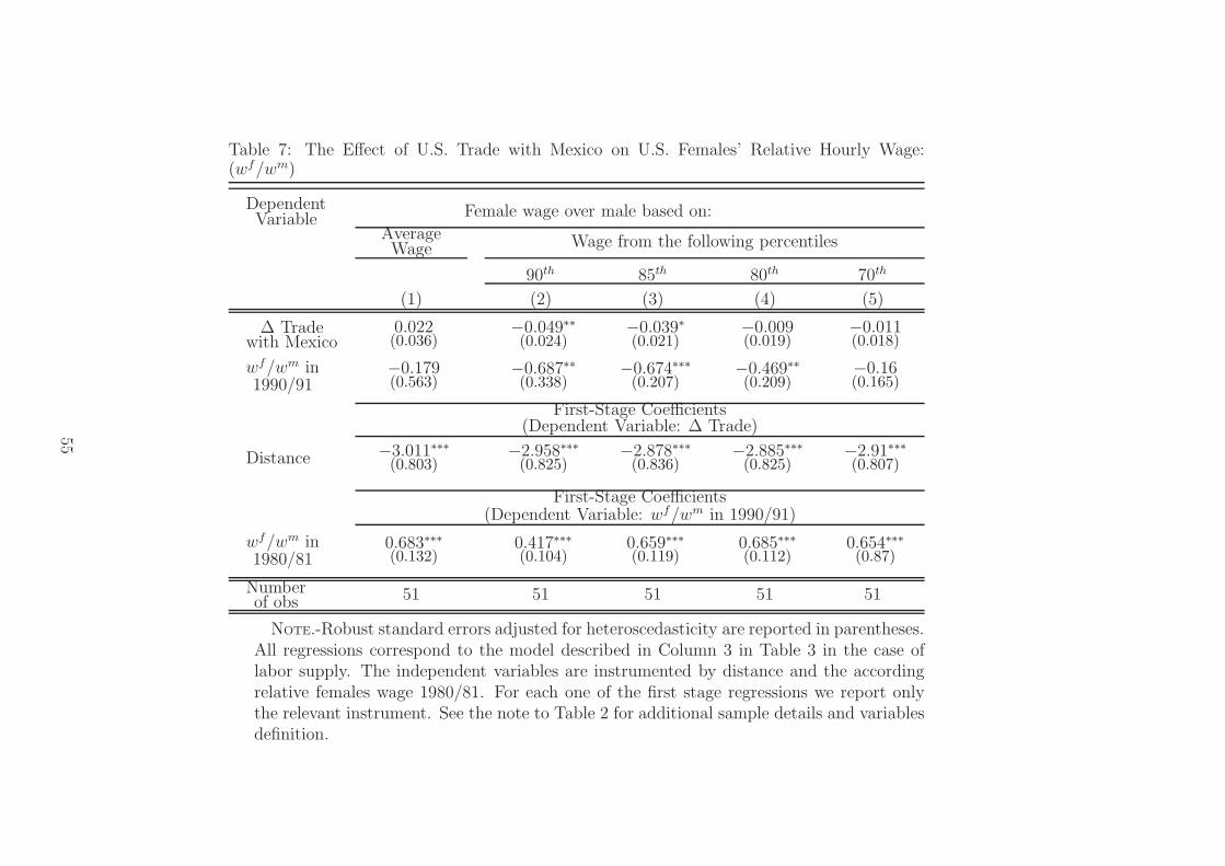
Table 7: The Effect of U.S. Trade with Mexico on U.S. Females’ Relative Hourly Wage:(wf/wm)

DependentVariable Female wage over male based on:

AverageWage Wage from the following percentiles

90th 85th 80th 70th

(1) (2) (3) (4) (5)

∆ Tradewith Mexico

0.022(0.036)

−0.049∗∗(0.024)

−0.039∗(0.021)

−0.009(0.019)

−0.011(0.018)

wf/wm in1990/91

−0.179(0.563)

−0.687∗∗(0.338)

−0.674∗∗∗(0.207)

−0.469∗∗(0.209)

−0.16(0.165)

First-Stage Coefficients(Dependent Variable: ∆ Trade)

Distance −3.011∗∗∗(0.803)

−2.958∗∗∗(0.825)

−2.878∗∗∗(0.836)

−2.885∗∗∗(0.825)

−2.91∗∗∗(0.807)

First-Stage Coefficients(Dependent Variable: wf/wm in 1990/91)

wf/wm in1980/81

0.683∗∗∗(0.132)

0.417∗∗∗(0.104)

0.659∗∗∗(0.119)

0.685∗∗∗(0.112)

0.654∗∗∗(0.87)

Numberof obs 51 51 51 51 51

NOTE.-Robust standard errors adjusted for heteroscedasticity are reported in parentheses.All regressions correspond to the model described in Column 3 in Table 3 in the case oflabor supply. The independent variables are instrumented by distance and the accordingrelative females wage 1980/81. For each one of the first stage regressions we report onlythe relevant instrument. See the note to Table 2 for additional sample details and variablesdefinition.

55

First Appendix

Falsification Test

In our falsification test we conduct the following triple difference exercise. We compare

the explanatory power of distance to Mexico for the change in female labor force participa-

tion in two different periods: first, 1990–2000, in which we observe a substantial increase in

U.S.-Mexican trade; and second, 1960–1970, when U.S.-Mexican trade was stagnant (Fig-

ure 3). We simply label these periods by “NAFTA episode” and “pre-NAFTA episode”

respectively. We employ the Integrated Public Use Microdata Series (IPUMS-USA) of the

decennial censuses data (Ruggles, Sobek, Alexander, Fitch, Goeken, Kelly Hall, King, and

Ronnander (2009)). This source provides us with employment data for men and women for

the years 1950, 1960 and 1970 for the pre-NAFTA episode, and 1980, 1990 and 2000 for the

NAFTA episode. Table 8 below summarizes these reduced form regressions of the change in

female labor force participation directly on distance in the two episodes and shows that dur-

ing the NAFTA episode the coefficients of distance are positive and significant while in the

pre-NAFTA episode are negative and not consistently significant. We read this as additional

support to the validity of our instrument.

56

Table 8: Explanatory Power of Distance on Female Labor Force Participation

Dependent Variable:Change in

Share ofHours Worked

RelativeEmployment

preNAFTA NAFTA

preNAFTA NAFTA

(1) (2) (3) (4)

distance −3.933∗∗∗(1.44)

2.703∗∗∗(0.562)

−4.423(4.572)

10.236∗∗∗(1.844)

Initial FLFP −0.009(0.111)

−0.544∗∗∗(0.08)

−0.217(0.134)

−0.736∗∗∗(0.125)

First-Stage Coefficients(Dependent Variable: Initial level for FLFP)

Lagged FLFP 0.675∗∗∗(0.085)

0.593∗∗∗(0.039)

0.753∗∗∗(0.047)

0.632∗∗∗(0.068)

Number of obs 42 51 42 51

NOTE.-Robust standard errors adjusted for heteroscedasticity are reported in paren-theses. In all regressions FLFP is regressed on distance and the initial level of FLFP.The dependent variables, relative employment described in Columns 3 & 4 is the ratio offemales employment over males employment. The initial level of FLFP is instrumentedby its lagged level. The pre-NAFTA period is 1960–1970 and the NAFTA period is 1990–2000. Lagged levels are 1950 and 1980, respectively. For the pre-NAFTA period part ofthe data are missing for 9 states, which are Alaska, Delaware, Hawaii, Idaho, Montana,North Dakota, South Dakota, Vermont and Wyoming. Restricting our NAFTA periodregressions to the same 42 states does not affect neither the magnitudes of coefficientsnor their significance. See the note to Table 2 for additional sample details and variablesdefinition.

57

Second Appendix

Proofs

Proof that 1/mt is bounded above. First observe that kt → ∞ means kt > ko so

that the second regime applies. Use (24) to confirm that κt → ∞ as kt → ∞ (else the

denominator in the brackets of the expression on the right turns negative). Finally, divide

equation (22) by καt to get

1− θ

θ

1

καρt

( abmt + [mt − (1− znt)] κ

−αt

1−mt + (1− znt)

)1−ρ

→ (1− α)a

b(kt → ∞).

Since this limit is positive, the term in brackets must approach infinity as kt → ∞ so that,

as limκt→∞ znt = 2γ, limkt→∞mt = 2(1 − γ) must hold. This proves that 1/mt is bounded

above.

Proof of Proposition 1. The proof of ”⇒” is immediate by rt = r∗t and (9).

For ”⇐” assume that κ∗

t = κt, which implies rt = p1,tαaκα−1t = p1,tαa (κ

∗

t )α−1 = r∗t and

wFt = p1,t(1− α)aκα

t = p1,t(1− α)a (κ∗

t )α = wF,∗

t . By X2,t > 0 we have l2,t + l∗2,t > 0. In case

l∗2,t, l2,t > 0 wMt = wM,∗

t follows from (10). In case l∗2,t = 0 this implies

wMt = p2,tb ≤ wM,∗

t .

At the same time l∗1,t = 1 implies

wM,∗t = p1,t((1− α)a(κ∗

t )α + b) = p1,t((1− α)aκα

t + b) ≤ wMt

so that wMt = wM,∗

t . In case l2,t = 0 switching Home and Foreign variables leads to wMt =

wM,∗t again.

58

Proof of Proposition 3. (i) By (16) it is sufficient to show ω∗

t ≤ ωt. Since free trade

implies l∗1,t > 0 and l2,t > 0 we have ωt = πtb/ [a (1− α) καt ] ≥ 1 + b/ [a (1− α) κα

t ] and

ω∗

t = 1 + b/ [a (1− α) (κ∗

t )α] ≥ πtb/ [a (1− α) (κ∗

t )α]. Combining these relations gives

ω∗

t

ωt

≤πt + ω∗

t

πt + ωt

and proves statement (i).

(ii) By (i) we have zn∗

t ≤ znt and distinguish two cases according to (16). The first,

where znt = 1 holds, gives with (39)

k∗

t+1

kt+1≥

wM,∗

wM≥

p2,tb

p2,tb= 1

(We used k∗

t+1 ≥ zwM,∗ for the first inequality and l2,t > 0 for the second.)

If, instead, znt < 1 holds, then (i) implies zn∗

t < 1 so that (39)

k∗

t+1

kt+1

=wF,∗

wF=

ωt

ω∗

t

wM,∗

wM≥

wM,∗

wM≥ 1

where we used (i) and (16) in the first inequality; the second inequality follows as above.

(iii) If znAt = 1 we have

kAt+1

kt+1≤

wM,A

wM=

pA2,tb

p2,tb≤ 1

If, instead, znAt < 1 then znt < 1 (from (34) as long as l1,t > 0 and mt > 0 otherwise) and

kAt+1

kt+1≤

wF,A

wF=

ωt

ωAt

wM,A

wM

For the case ωt ≤ ωAt (or πt ≤ πu in Figure 2) this proves the claim. If instead ωt > ωA

t we

use κt = kt/(1− znt) and (16) to write

κt

(

1− γ

(

1 + πtb/a

1− ακ−αt

))

= kt

59

and take implicit derivatives

dκt

dπt= κt

1

1− α

γ

(1− γ)a/bκαt − γπt

At the same time (40) leads to

dp1,tdπt

= −p1− ρ

1−ρ

1,t

(

1− θ

πt

)1

1−ρ

Thus,

d

dπtln (p1,tκ

αt ) =

α

1− α

γ

(1− γ)a/bκαt − γπt

−

(

(

θ

1− θ

) 1

1−ρ

πρ

1−ρ

t + π−ρ1−ρ

t

)−1

π−1t

A sufficient condition for this expression to be positive is

α

1− α

γ

π−1t (1− γ)a/bκα

t − γ>

1(

θ1−θ

)1

1−ρ πρ

1−ρ

t + 1

or with ωt = πtb/ [a (1− α)καt ]

α

1− α

γ1−γ1−α

1ωt

− γ>

1(

θ1−θ

)1

1−ρ πρ

1−ρ

t + 1

Since ωt > 1 and πt > 1 this condition is satisfied whenever

αγ

1− γ − (1− α)γ>

1(

θ1−θ

)1

1−ρ + 1

or (θ/(1− θ))1

1−ρ ≥ (1− 2γ) /(αγ) holds, proving the statement (iii).

(iv) Notice with Proposition 2 (i) that the first case, zn∗

t < 1, implies k∗

t+1/k∗,At+1 =

p1,t(κ∗

t )α/(p∗,A1,t (κ

∗,At )α). If zn∗

t = 1, instead, k∗

t+1/k∗,At+1 = p1,t ((1− α)aκ∗

t + b) /(p∗,A1,t ((1 −

α)aκ∗,At +b)). Now, inequality (37) and expression (40) for the price p

(∗,A)1,t imply p1,t/p

∗,A1,t ≤ 1.

60

Further, by m∗,At ≤ m∗

t we have κ∗,At ≥ κ∗

t and thus

k∗

t+1/k∗,At+1 ≤

(

κ∗

t/κ∗,At

)α

Similarly, we compute for znt < 1 that kt+1/kAt+1 = p1,tκ

αt /(p

A1,t(κ

At )

α) while for znt = 1

kt+1/kAt+1 = p1,t ((1− α)aκα

t + b) /(pA1,t((1 − α)a(κAt )

α + b)) holds. By (37) and expression

(40) we have p1,t/pA1,t ≥ 1. Further, by mA

t ≥ mt we have κAt ≥ κt and thus

kt+1/kAt+1 ≥

(

κt/κAt

)α

Combining both inequalities leads to

k∗

t+1/k∗,At+1

kt+1/kAt+1

≤

(

κ∗

t/κ∗,At

κt/κAt

)α

=

(

m∗,At /m∗

t

mAt /mt

)α

Using again m∗,At ≤ m∗

t and mAt ≥ mt shows that the expression on the right falls weakly

short of unity, which proves the statement.

61

Third Appendix

A Generalization of the Static Result

A The General Framework

The framework of our model economy is extremely general. On the preference side we assume

that female labor supply is a decreasing function of the gender wage gap, while supply of male

labor is inelastic. Regarding production technologies, we merely assume constant returns to

scales in two tradable sectors. Moreover, female labor, male labor and capital are distinct

factors of production. We thus deal with the – slightly unconventional – case of a two-good,

three-factor model. This generality on the modeling framework requires that we adopt an

open economy framework and formulate our results in terms of exogenous changes in good

prices.

A.1 The Setup

Regarding the framework of our model we try to be quite general. On the preference side

we assume that female labor supply is a decreasing function of the gender wage gap, while

supply of male labor is inelastic. Regarding production technologies, we merely assume

constant returns to scales in two tradable sectors. Moreover, female labor, male labor and

capital are distinct factors of production. We thus deal with the – slightly unconventional –

case of a two-good, three-factor model.

A.1.1 Production

Firms transform three different factors K, F and M into two distinct consumption goods

Q1 and Q2, using the technologies

Qi = Gi(K,F,M) i = 1, 2. (A-1)

62

The functions Gi exhibit constant returns to scale, i.e., they are homogeneous of degree one.

We assume that the functions Gi are twice continuously differentiable and satisfy

GiX > 0; Gi

XY ≥ 0 for X 6= Y ; GiXX < 0 (A-2)

where subscripts stand for partial derivatives and X, Y ∈ {K,F,M}. Finally, the usual

Inada conditions are assumed to hold.

Sectors differ in their demand for F -type labor relative to M-type labor. Without loss of

generality the first sector is relatively more intensive in F , i.e.44

F1/F > M1/M (A-3)

holds under firm optimization, provided that Q1, Q2 > 0 is satisfied.

A.1.2 Factors

The variable K stands for physical capital. For the variables F and M different interpreta-

tions are possible. First, F and M may stand for female and male labor, respectively. Under

positive output in both sectors the Inada conditions imply positive employment of all factors

in all industries. Hence, the male and female wage, denoted as wM and wF , respectively, are

equal to the marginal product of corresponding labor, i.e.

wM = p1G1M = p2G

2M and wF = p1G

1F = p2G

2F (A-4)

holds. Alternatively, the factor F may stand for ”brain” or mental inputs, while M stands

for ”brawn” or physical labor as in the main body of the paper. Male and female workers

are endowed with these two distinct types of factors at different proportions. We can think

of male workers being endowed with one unit of F and one unit of M , while female workers

44With F = F1 + F2 and M = M1 +M2 it is immediate to check that this condition is equivalent to thecondition F1/F2 > M1/M2 and thus to the condition F1/M1 > F2/M2, which may be more common.

63

owe one unit of F but β < 1 units of M . In this case, the contribution of mental labor

rewards are relatively higher for female than for male workers. Whenever interior solutions

prevail (i.e., workers of both genders are employed in both sectors) wage equalization requires

p1 (G1M +G1

F ) = p2 (G2M +G2

F ) and p1 (βG1M +G1

F ) = p2 (βG2M +G2

F ), which constitutes a

system equivalent to (A-4). We will focus on interior solutions, so that both interpretations

of F and M are, in terms of factor allocation, formally equivalent.

A.1.3 Preferences

Individuals consume the two goods Q1 and Q2. Concerning labor supply, we assume that

(i) male labor is entirely inelastic and (ii) female labor supply depends only on the ratio of

female to male wages, ω.

By the second assumption, we can write supply of female over male working hours as

Rs(ω). (A-5)

The superscript s indicates supply and ω stands for the ratio of F -factor price over M-factor

price. The function R is assumed to be increasing in ω.

A.2 Inelastic Factor Supply

We begin our analysis by considering an economy with inelastic factor supply. Denoting the

vector of factor endowments with Z = (K, F ; M)t, we write Z = (K1, F1,M1)t for the vector

of factors employed in the Q1-sector.

A.2.1 Factor Allocation

Competitive firms maximize their profits. In terms of factor allocation, such maximization

is equivalent to the maximization of total revenues (see Mas-Colell, Whinston, and Green

64

(1995)):

maxZ

p1G1(Z) + p2G

2(

Z − Z)

(A-6)

We assume that the solution to (A-6) is unique and interior and we denoted it by Z∗(Z).

Further, we denote wX for the reward of factor X (wM and wF are defined in (A-4), the

interest rate wK is defined correspondingly) and formulate the following lemma.

Lemma A.1 Assume prices pi are constant, then (A-2) implies

d

dXln

(

wX

wY

)

< 0 X, Y = K,M,F Y 6= X (A-7)

Proof. (i) Let X, Y, ξ ∈ {K,F,M} and ξ 6= Y . Show that Y1/X1 and Y2/X2 cannot

simultaneously increase in ξ. Assume that they do, i.e.

Y1/Y1 > X1/X1

−Y1/(Y − Y1) > (δXξ − X1)/(X −X1)(A-8)

holds, where dots indicate derivatives w.r.t. ξ and the Kronecker delta is defined as usual as

δξξ = 1, δXξ = 0 if X 6= Z.

Consider now the two cases Y1/X1 >(

Y − Y1

)

/(

X −X1

)

and Y1/X1 <(

Y − Y1

)

/(

X −X1

)

.

In the first case

Y1/X1 >(

Y − Y1

)

/(

X −X1

)

, (A-9)

the second inequality in (A-8) then implies

Y1/Y1 <(

−δXξ + X1

)

/X1

contradicting the first inequality in (A-8).

Consider the second case, were (A-9) is violated, so that the second inequality of (A-8)

−Y1/Y1 > (δXξ − X1)/X1

65

contradicting the first inequality in (A-8).

(ii) Let Y,X ∈ {K,F,M} and Y 6= X and show that at most one of the four ratios Yi/Xi

(i = 1, 2) increases in X. Take X = M and show that at most one of K1/M1, K2/M2, F1/M1

and F2/M2 increases in M . All other cases follow identically.

By homogeneity of degree zero of the vector of derivatives∇Gi = (dGi/dK, dGi/dF, dGi/dM)t,

the first order conditions to (A-6) can be written as

p1∇G1

K1/M1

1

F1/M1

= p2∇G2

K2/M2

1

F2/M2

Assume that K1/M1 and F1/M1 increase in M . By (i) this implies that K2/M2 and F2/M2

decrease in M . Hence, by (A-2), p1G1M increases and p2G

2M decreases. This contradicts the

optimality condition p1G1M = p2G

2M . Assume, instead, that K1/M1 and F2/M2 increase in

M , so that K2/M2 and F1/M1 decrease. Again by (A-2), p1G1F increases and p2G

2F decreases,

contradicting optimality. Switching indices covers the remaining cases.

(iii) Let X ∈ {K,F,M} and show dGiX/dX < 0. Take X = M and show dGi

M/dM < 0; all

other cases follow identically. By (ii), for each i = 1, 2, at least one of the ratios Ki/Mi and

Fi/Ki decreases in M . By (A-2) and

GiM

(

(Ki, Fi,Mi)t) = Gi

M

(

(Ki/Mi, Fi/Mi, 1)t)

this implies that GiM decreases in M .

(iv) Let X, Y ∈ {K,F,M} and Y 6= X and show dGiY /dX > 0. Take X = M and and

Y = F ; all other cases follow identically. Show dGiF/dM > 0. Applying (i) to Ki/Fi and

Fi/Ki shows that the ratio Ki/Fi increases in M for exactly one i. Let wlog F1/K1 increase

66

and F2/M2 decrease in M . Now, write the first order conditions to (A-6) as

p1∇G1

1

M1/K1

F1/K1

= p2∇G2

1

M2/K2

F2/K2

By (i), Mi/Ki increases for at least one i. In case that M1/K1 increases and M2/K2 de-

creases, (A-2) implies that G1K increases while G2

K decreases, contradicting optimality. If

M1/K1 decreases and M2/K2 increases, then G1F decreases while G2

K increases contradicting

optimality. Hence, Mi/Ki increase for i = 1, 2. Therefore, G2F increases in M .

The lemma states that an increase in aggregate supply of one factor decreases its price

relative to the price of all other factors. Thus, the decreasing returns to each factor on the

industry level translate, quite intuitively, to decreasing returns to the same factor on the

aggregate, economy-wide level.

A.2.2 Effects of Capital Accumulation: the ”Complementarity-Condition”

Having derived some intuitive results in our setup of a small open economy, we now impose

our key assumption on the modeling framework. Specifically, we assume that an increase in

the capital stock raises the rewards of F more than that of M :

d

dKln

(

wF

wM

)

> 0. (A-10)

Following Goldin (1990), an important branch of the economics of demography have argued

that the accelerating capital accumulation has helped to closed the gender wage gap. Refer-

ring to her seminal contribution, we will refer to this inequality as the “Complementarity-

Condition”.45

It will prove useful to formulate the relations between equilibrium factor allocation and

45Below, we reformulate the ”Complementarity-Condition” in terms of factor price elasticities.

67

factor prices in terms of demand elasticities. Doing so, however, we need to account for

the fact that under technologies with constant return to scale, the good- and factor-prices

determine factor demand uniquely only up to a scaling factor. To regain unique factor

demand, we thus consider relative factor demand relative to male labor: k = K/M and

f = F/M . The relation between factor allocation and factor prices is then

∆wK

∆wF

≡

wK − wM

wF − wM

=

αKk αK

f

αFk αF

f

k

f

(A-11)

where we have set X = dX/X and αXy = [d (wX/wM) /dy] / [(wX/wM) /y] for X ∈ {K,F}

and y ∈ {k, f}.

In the terminology thus defined, the “Complementarity-Condition” (A-10) becomes

αFk > 0. (A-12)

Moreover, setting X = K,F and Y = M in inequality (A-7) and using the system (A-11)

translates into the following condition

αXx < 0 for (X, x) ∈ {(K, k), (F, f)}. (A-13)

Finally, setting X = M and Y = K,F in inequality (A-7) and using (A-11) leads to46

−αYk − αY

f > 0 Y = K,F. (A-14)

Together, these conditions imply that the determinant of the 2 × 2 matrix from (A-11) is

positive

46Notice that, by definition of k = K/M and f = F/M , a one percent increase in M is equivalent to asimultaneous one percent decrease in k and f .

68

Lemma A.2

D = αKk α

Ff − αK

f αFk > 0.

Proof. Consider the two cases αKf < 0 and αK

f > 0. Case I: if αKf < 0 this statement is true

by (A-12) and (A-13) above.

Case II: if αKf > 0, instead, (A-14) with Y = K implies −αK

k > αKf > 0. Hence,

−αKk α

Ff < αK

f αFf since αF

f < 0 by (A-13). This implies for the determinant in (A-11)

αKk α

Ff − αK

f αFk > −αK

f αFf − αK

f αFk = αK

f (−αFf − αF

k ) > 0

where the last step follows by αKf > 0 and (A-14).

We can thus invert the system (A-11), writing

k

f

=

σkK σk

F

σfK σf

F

∆wK

∆wF

(A-15)

According to Cramer’s rule, σkK = αF

f /D, σfF = αK

k /D, σkF = −αK

f /D and σfK = −αF

k /D

hold so that the above inequalities on the αXy are

σfK < 0 and σy

Y < 0 and |σyY | > |σy

X | (Y,X = K,F ; X 6= Y ). (A-16)

By definition, σyX is the economy-wide elasticity of relative demand with respect to the

relative factor price, i.e.

σyX =

(wX/wM)

y

dy

d (wX/wM)X = K,F y = k, f. (A-17)

Hence the first of the inequalities in (A-16) constitutes the “Complementarity-Condition”

(A-10) expressed in terms of factor demand elasticities. The translation into factor price

elasticities shows that the ”Complementarity-Condition” is equivalent to a relatively strong

69

economy-wide complementarity between capital and female labor (σfK < 0). For a better

understanding of the equivalence between (A-10) and (A-16), observe that, as more capital

K is added to the system, demand for female labor F must rise so as to increase its factor

reward relative to M . This rise in demand for female labor F is achieved by a strong

complementarity between F and K.

A.2.3 Capital Intensity

Having stated our main assumption concerning wage-raising capital accumulation, we now

turn to an important intermediate result, which concerns relative capital intensities of the

two sectors.

Lemma A.3 If (A-2), (A-3) and (A-10) hold and Z∗(Z), is interior, then

K1/K > F1/F (A-18)

Proof. As the solution to (A-6) is interior, we can write wX = p1G1X (X = K,M,F ).

Observe that the uniqueness of the solution to (A-6), together with homogeneity of degree

one of Gi, implies linear independence of Z∗ and Z−Z∗. Further, at constant pi, an increase

of the vector Z in the directions Z∗ or Z − Z∗ leaves factor prices unchanged. Thus, factor

prices are constant under a marginal change of Z in the direction ξ = Z∗ − γ(

Z − Z∗)

for

all γ ∈ R. The particular choice γ = F1/(F − F1) implies ξ = (ξ1, 0, ξ3). Hence,

(

ξ1d

dK+ ξ3

d

dM

)

ln

(

G1F (Z∗)

G1M (Z∗)

)

= 0

holds. Therefore, by (A-7) with X = M and Y = F and (A-10), we infer that ξ1 and ξ3

have opposite sign. By (A-3) we have

ξ3 = M1 − (M −M1)F1/(F − F1) < 0.

70

Therefore, ξ1 = K1 − (K −K1)F1/(F − F1) > 0 holds, implying (A-18).

The lemma shows that Q1-production is relatively more K-intensive than F -intensive.

Together with (A-3) we then have

K1

K −K1

>F1

F − F1

>M1

M −M1

(A-19)

Interestingly, in a two-sector world Goldin’s statement implies that the sector, which is in-

tensive in female labor (relative to male labor), is necessarily even more intensive in capital.

An intuition for this result obtains from the following considerations. Assume that X2-

production were K-intensive, violating (A-18), while (A-3) still implied that X1-production

is F -intensive. Under these assumptions, increases in the capital stock would spur produc-

tion of the X2-sector.47 In terms of factor prices, this advantage to the X2-sector should

benefit mainly the factor it uses most intensively – i.e., male labor. But this is ruled out by

assumption (A-10). – It must be stressed that this explanation provides not more than an

intuition. As shown further below, simple arguments relating factor intensities to movement

of relative factor prices are not admissible. Instead, an important role is played by factor

demand elasticities.

A.2.4 Price Changes

To analyze the effects of changes in goods prices, we adapt and extend the results from

Jones and Easton (1983) to our current setting. For the time being, we keep the assumption

that factors are inelastically supplied. We start by introducing the notation aXj for the

(equilibrium) input requirement of factor X = K,F,M to produce one unit of good j = 1, 2.

47Hence, a Rybczynski-like effect is implicitly assumed to operate. The Rybczynski efffect is dual to theStolper-Samuelson effect, which the present paper shows not to be holding for male and female labor. Noticethat the fact that a Rybczynski-like efffect operates for capital is no contradiction to the key point of thepaper.

71

With this notation, inequalities (A-19) become

aK1

aK2>

aF1

aF2>

aM1

aM2

Multiplying each aXj by the according factor price wX and dividing by the respective good

prices, pj, leads to the expenditure share of factor X in sector j, which we denote by θXj =

wXaXj/pj. Hence, the condition above is equivalent to

θK1

θK2

>θF1

θF2

>θM1

θM2

(A-20)

In a competitive economy with constant returns to scale

∑

XaXjwX = pj j = 1, 2 (A-21)

is satisfied as long as both goods are produced in positive quantities.

Being interested in a change in relative price changes we next consider a marginal increase

in pj (j = 1, 2). Differentiating expression on the left of (A-21) with respect to pi, we apply

the envelope theorem to cost minimization (taking partial derivatives of wX only), which

leads to∑

XθXjwX = δij j = 1, 2 (A-22)

where δii = 1, δij = 0 (j 6= i) and y = (dy/dp1)p1/y as defined above.

Finally, the second line of the system (A-15) reads

σfK (wK − wM) + σf

F (wF − wM) = f . (A-23)

72

Combining now (A-22) and (A-23) leads to

θK1 θF1 θM1

θK2 θF2 θM2

σfK σf

F −σfK − σf

F

wK

wF

wM

=

p1

p2

f

(A-24)

We will now analyze a one percentage increase in p1 at constant factor supply. To this

aim, consider the exogenous change (p1, p2, f)t = (1, 0, 0)t in (A-24). To solve this specific

system, denote the determinant of the 3×3 matrix by ∆ and use Cramer’s Rule to compute

(setting σfM ≡ −σf

K − σfF )

wK = ∆−1 det

1 θF1 θM1

0 θF2 θM2

0 σfF σf

M

= ∆−1[

σfMθF2 − σf

F θM2

]

wF = ∆−1 det

θK1 1 θM1

θK2 0 θM2

σfK 0 σf

M

= −∆−1[

σfMθK2 − σf

KθM2

]

wM = ∆−1 det

θK1 θF1 1

θK2 θF2 0

σfK σf

F 0

= ∆−1[

σfF θK2 − σf

KθF2

]

Using∑

X θXj = 1 and∑

X σfX = 0 (from σf

M ≡ −σfK − σf

F ) leads to

wK = −∆−1[

σfKθF2 + σf

F (1− θK2)]

wF = ∆−1[

σfF θK2 + σf

K (1− θF2)]

(A-25)

wM = ∆−1[

σfF θK2 − σf

KθF2

]

73

Employ again∑

X θXj = 1 and∑

X σfX = 0 to compute the determinant ∆:

∆ = det

θK1 1 θM1

θK2 1 θM2

σfK 0 −(σf

K + σfF )

= (θM2 − θM1)σKK − (θK1 − θK2) (σ

KK + σK

F ) (A-26)

Combining (A-25) and (A-26) leads to

d

dp1ln

(

wF

wM

)

=σfK

(θF1 − θF2)σfK − (θK1 − θK2)σ

fF

(A-27)

This identity implies that female relative wages wF/wM are decreasing in p1 if and only

if the expression on the right is negative. Now, using (A-20) together with∑

X θXj = 1,

implies θK1 > θK2. Since further σfK < 0 holds by (A-16), we can state that a necessary and

sufficient condition for the expression above to be negative is

θF1 − θF2

θK1 − θK2≤

σfF

σfK

Finally, the condition formulated in (A-16) implies that the expression on the right exceeds

one, while the expression on the left falls short of unity, by (A-20). This proves the following

statement.

Proposition A.1 If (A-10) holds, then

d

dp1ln

(

wF

wM

)

< 0

The proposition shows that, under the “Complementarity-Condition” (A-10) the intuition

based on the Stolper-Samuelson effect of a two-good two-factor economy never generalizes

to F and M in the current setting. Any price increase of the good whose production uses F

more intensively than M , decreases the reward for F relative to that of M .

The key condition, of course, is the “Complementarity-Condition”. In absence of it,

74

the usual Stolper-Samuelson based intuition concerning the interplay of factor intensities,

international specialization and relative factor prices may go through.

A.3 Elastic F -Supply

It is now quick to translate these findings to a framework with elastic F -supply. The ratio

of female wage over male wage is G1F/G

1M . Therefore, the supply of female labor over male

labor Rs from (A-5) is a function of relative factor prices ω = wF/wM = GiF/G

iM . As we

have assumed above, the function Rs(ω) is increasing (see (A-5) in subsection A.1.3).

Turning now to the demand for F , we maintain the assumption that the factorsK andM

are in inelastic supply. Thus, applying (A-7), we infer that an increase in F lowers the ratio

of factor prices ω = wF/wM . Inverting this relation implies that demand for F , denoted by

Rd(ω), is a decreasing function of ω.

The functions Rs and Rd are plotted in Figure 5 as solid lines – Rs as an increasing

function and Rd as a decreasing function of ω. The figure also depicts the effects of an

increase in p1, which, by Proposition 2, decreases the ratio wF/wM for any given level of F .

This means that the increase of p1 shifts the Rd-schedule to the left. Since the Rs-schedule

is unaffected by the price change, the equilibrium employment of F drops from F ∗ to F ∗∗.

Lemma A.4 If (A-10) holds, female labor shares drop whenever p1/p2 rises.

The statement of lemma A.4 reformulates our main result from Proposition A.1. To

further translate it to the terminology of trade theory, we spell it out in terms international

specialization.

A.4 International Specialization

Up to this stage, we have considered exogenous price changes and their consequence for

a small open economy. In the following paragraphs, we will analyze the patterns of spe-

cialization that arise in equilibrium and their effect on female labor force participation.

75

F*

F**

Rd

Rs

F

Figure 5: F-type labor - demand and supply.

Nevertheless, we refrain from explicitly solving the general equilibrium of a world economy

of many countries instead. Specifically, we assume that the world economy consists of a

collection of countries of the type described above. We keep being general in terms of tech-

nologies and preferences over consumption goods, assuming that each country faces a set of

production technologies (A-1) with which to produce the two consumption goods and indi-

viduals have preferences that give rise to F -supply (A-5). We do not require technologies

or preferences to be identical across countries. This implies that international specialization

may be driven by differences in technologies, in the per-household capital stocks, in demand

for the consumption goods, or by a combination of all.

There are only two key assumptions we make. First, we assume that the “Complementarity-

Condition” (A-10) holds for each of the countries. Second, a drop in the relative price of

a good is associated with a drop in this country’s excess supply of the relevant good. Put

differently, the Marshall-Lerner stability conditions are met by assumption.

Now, we say that a country intensifies specialization in good Xi if and only if its excess

supply of Xi rises. With this terminology, the statement of Lemma A.4 can be reformulated

as follows: given that the ”Complementarity-Condition” (A-10) holds, female labor shares

76

drop in countries that intensify specialization on sectors intensive in female labor.

Notice that this statement holds, whether the shift in excess supply and the associated

price change originates from a removal of trade barriers, from demand shifts or from (foreign)

technological change. Since all effects of trade ultimately operate through a shift in good

prices, our result is independent of the actual source of the international pattern of special-

ization. In this sense, we claim that our finding, which runs counter to the well-established

intuition derived from the Stolper-Samuelson Theorem, is very general.

77