Internship Rolls-Royce DeutschlandAeroacoustics and Noise01.02.2015 - 31.05.2015

N.J.G. van Dijk (s1006339)

MSc Internship Report

N.J.G. van Dijk

s1006339, n.j.g.vandijk@student.utwente.nl

Company details:Rolls-Royce Deutschland Ltd & Co KGEschenweg 11, Dahlewitz15827 Blankenfelde-Mahlow, Germany

Aeroacoustics and Noise, ED-63

Mentor 1: M. Lehmann, Martin.Lehmann@Rolls-Royce.comMentor 2: C. Richter, Christoph.Richter@Rolls-Royce.comMentor 3: M. Rose, Marco.Rose@Rolls-Royce.comMentor 4: M. Wichmann, Maria.Wichmann@Rolls-Royce.com

Supervisor: F. Holste, fredi.holste@rolls-royce.com

Internship period: 01.02.2015 - 31.05.2015

University of Twente

Faculty of Engineering Technology (CTW)

Engineering Fluid Dynamics

Supervisor: H.W.M. Hoeijmakers, h.w.m.hoeijmakers@utwente.nl

Preface

As part of the study Mechanical Engineering and the specialisation Engineering Fluid Dynamics studentshave to perform an internship to put gained knowledge into practice. Those internships are often per-formed at universities or companies to gain insight in a working environment. It is also a great opportunityto get a taste of the international engineering life by going abroad and to greatly improve social skills.Therefore, I chose to perform my intership at Rolls-Royce Deutschland for the period of four monthsbetween February and May 2015.

During my time at Rolls-Royce Deutschland I mainly worked on acoustics at the Aeroacoustics and Noisedepartment under the supervision of Fredi Holste. My main assignment consisted of the development of anoise prediction tool for design of experiment studies in Matlab for Martin Lehmann. Besides that, I alsoassessed the acoustic lined area and acoustic impedance realised by a current production standard BR700series bypass duct for Christoph Richter and a small weather study for an engine test bed for Marco Rose.

I would like to thank professor Harry Hoeijmakers of the Engineering Fluid Dynamics department, whichis my university supervisor, for arranging the internship at Rolls-Royce Deutschland. I would like to thankall people of the Aeroacoustics and Noise department for the great time I had during my internship andin special Fredi, for his supervision, Martin, Christoph and Marco for the guidance of their assignmentsand Maria Wichmann for her overall guidance throughout my internship.

Niek van Dijk

i

Contents

List of Figures iii

List of Tables iv

1 Introduction 1

2 Assignment 1: Noise prediction software 22.1 Assignment description . . . . . . . . . . . . . . . . . . . . . . . . . . . . . . . . . . . . . . 22.2 Overview of noise prediction . . . . . . . . . . . . . . . . . . . . . . . . . . . . . . . . . . . 22.3 Performance data and noise testing conditions . . . . . . . . . . . . . . . . . . . . . . . . . 32.4 Program process of vn02DoE . . . . . . . . . . . . . . . . . . . . . . . . . . . . . . . . . . 42.5 Initial state versus current state of the developed program . . . . . . . . . . . . . . . . . . 52.6 Software capabilities . . . . . . . . . . . . . . . . . . . . . . . . . . . . . . . . . . . . . . . 7

2.6.1 Example of usage and results . . . . . . . . . . . . . . . . . . . . . . . . . . . . . . 72.6.2 Alternating/changing parameters . . . . . . . . . . . . . . . . . . . . . . . . . . . . 82.6.3 GUI options . . . . . . . . . . . . . . . . . . . . . . . . . . . . . . . . . . . . . . . . 92.6.4 Warnings and errors . . . . . . . . . . . . . . . . . . . . . . . . . . . . . . . . . . . 9

2.7 Process development and basic code structure . . . . . . . . . . . . . . . . . . . . . . . . . 102.8 Documentation and test log . . . . . . . . . . . . . . . . . . . . . . . . . . . . . . . . . . . 11

2.8.1 User guide . . . . . . . . . . . . . . . . . . . . . . . . . . . . . . . . . . . . . . . . . 112.8.2 Developer guide . . . . . . . . . . . . . . . . . . . . . . . . . . . . . . . . . . . . . 112.8.3 Test log for tool validation . . . . . . . . . . . . . . . . . . . . . . . . . . . . . . . 11

2.9 Conclusion . . . . . . . . . . . . . . . . . . . . . . . . . . . . . . . . . . . . . . . . . . . . 11

3 Assignment 2: Bypass duct acoustic lined area assessment 123.1 Assignment description . . . . . . . . . . . . . . . . . . . . . . . . . . . . . . . . . . . . . . 123.2 Acoustic lined area . . . . . . . . . . . . . . . . . . . . . . . . . . . . . . . . . . . . . . . . 123.3 Report . . . . . . . . . . . . . . . . . . . . . . . . . . . . . . . . . . . . . . . . . . . . . . . 13

3.3.1 Introduction . . . . . . . . . . . . . . . . . . . . . . . . . . . . . . . . . . . . . . . 133.3.2 Measurement of realised lined area in a BR700 series bypass duct . . . . . . . . . . 143.3.3 Impedance measurements at BR700 series bypass duct . . . . . . . . . . . . . . . . 17

4 Assignment 3: Weather data analysis for engine noise testing 274.1 Assignment description . . . . . . . . . . . . . . . . . . . . . . . . . . . . . . . . . . . . . . 274.2 Weather analysis . . . . . . . . . . . . . . . . . . . . . . . . . . . . . . . . . . . . . . . . . 28

5 Reflection 30

6 Appendix 31

ii

List of Figures

2.1 Basic flow diagram describing vn02DoE’s internal process. . . . . . . . . . . . . . . . . . . 32.2 Noise certification reference locations. . . . . . . . . . . . . . . . . . . . . . . . . . . . . . 42.3 Flow diagram describing the creation of vn02’s input files. . . . . . . . . . . . . . . . . . . 52.4 Initial state of vn02 at start of internship. . . . . . . . . . . . . . . . . . . . . . . . . . . . 52.5 Current state of vn02 at end of internship. . . . . . . . . . . . . . . . . . . . . . . . . . . . 62.6 Result example for 294 cycles. . . . . . . . . . . . . . . . . . . . . . . . . . . . . . . . . . . 8

3.1 Inner surface bypass duct with marked blocked areas. . . . . . . . . . . . . . . . . . . . . 143.2 Percentages of acoustic liner and blocked area, old (current model). . . . . . . . . . . . . . 163.3 Percentages of acoustic liner and blocked area, new. . . . . . . . . . . . . . . . . . . . . . 163.4 B&K WA1599 type impedance tube and equipment. . . . . . . . . . . . . . . . . . . . . . 173.5 Resistance vs. velocity, 7th point of a circular measurement at the rear end of the bypass

duct. . . . . . . . . . . . . . . . . . . . . . . . . . . . . . . . . . . . . . . . . . . . . . . . . 193.6 Effective hole diameter, scaled. . . . . . . . . . . . . . . . . . . . . . . . . . . . . . . . . . 213.7 Effective porosity, scaled. . . . . . . . . . . . . . . . . . . . . . . . . . . . . . . . . . . . . 223.8 POA vs. hole diameter, scaled. . . . . . . . . . . . . . . . . . . . . . . . . . . . . . . . . . 223.9 POA histogram, scaled. . . . . . . . . . . . . . . . . . . . . . . . . . . . . . . . . . . . . . 233.10 C-Rear 128dB, real part impedance ratio. . . . . . . . . . . . . . . . . . . . . . . . . . . . 233.11 Average impedance ratios per sound level with predictions, real part. . . . . . . . . . . . . 243.12 Average impedance ratios per sound level with predictions, imaginary part. . . . . . . . . 25

4.1 Test bed Stennis. . . . . . . . . . . . . . . . . . . . . . . . . . . . . . . . . . . . . . . . . . 274.2 Weather study Stennis. . . . . . . . . . . . . . . . . . . . . . . . . . . . . . . . . . . . . . 29

6.1 Effective hole diameter, uncorrected. . . . . . . . . . . . . . . . . . . . . . . . . . . . . . . 316.2 Effective porosity, uncorrected. . . . . . . . . . . . . . . . . . . . . . . . . . . . . . . . . . 316.3 POA vs. hole diameter, uncorrected. . . . . . . . . . . . . . . . . . . . . . . . . . . . . . . 32

iii

List of Tables

3.1 Blocked areas and total bypass duct surface. . . . . . . . . . . . . . . . . . . . . . . . . . . 153.2 Theoretical, average hole diameter and porosity values after scaling and excluding C-Rear 7. 21

4.1 Weather condition limits for noise testing. . . . . . . . . . . . . . . . . . . . . . . . . . . . 284.2 Certification tests. . . . . . . . . . . . . . . . . . . . . . . . . . . . . . . . . . . . . . . . . 28

6.1 Theoretical, average hole diameter and porosity values, uncorrected. . . . . . . . . . . . . 326.2 Theoretical, average hole diameter and porosity values after scaling. . . . . . . . . . . . . 32

iv

1 Introduction

The internship is performed within the Aeroacoustics and Noise department at Rolls-Royce Deutschland,at the headquarter located in Dahlewitz. ”RRD is Germany’s only fully certified engine manufacturer withcomplete systems capability for modern civil and militairy turbine engines. The site in Dahlewitz hostsRolls-Royces global headquarter for the Civil Small & Medium Engines business. RRD is certified for thedevelopment, assembly, testing, monitoring and maintenance of medium and small engines, powering e.g.Gulfstream and Bombardier business jets. More than 6,000 engines have been delivered from Dahlewitz todate. The site is also hosting a testbed for development tests of large engines, e.g. the Trent XWB, andthe Mechanical Test Operations Centre.”1

During my internship I performed three assignments. The first assignment consisted of the design andrefinement of a noise prediction tool with a graphical user interface in Matlab. The tool was mainly de-signed for performing complex parameter studies, or so called design of experiment studies. Also, for thisassignment an user guide and developer guide have been made and a comprehensive test log for validationof the implemented functions within the tool. The test procedure is very generic and can be used for othertools as well.

Secondly, acoustic impedance measurements were performed and evaluated on an acoustic liner for ascraped BR700 series bypass duct. Thirdly, a small assignment was performed on processing weather datato find suitable time slots for engine noise testing.

1http://www.rolls-royce.com/worldwide-presence.aspx#/our-contact/Germany

1

2 Assignment 1: Noise prediction software

2.1 Assignment description

The first assignment consists of the development of a noise prediction tool, called vn02DoE , in Mat-lab. The purpose of the tool is to perform design of experiment studies (DoE) based on another noiseprediction tool, called vn02 (see section 2.2 for more information about vn02), with varying performanceor geometry parameters for various engine configurations. These studies give insight on change in noiselevels for the varying parameters for different noise sources. Basically, the tool automatically performsvn02 calculations for all the different configurations provided and displays the results for an easy compar-ison between different engine configurations. More details on the internal processes are given in section 2.6.

Initially, the tool was in an early state capable of running the vn02 noise prediction software for oneconfiguration, but not fully functional. Both the graphical user interface (GUI) and underlying calculationsand manipulations were incomplete to perform complete design of experiment studies. This assignmentwas very open at the start of the internship, by adding tasks on a weekly and sometimes daily basis. Thestarting point was to get familiar with GUI programming in Matlab, which is one of the major parts formaking the tool fully functional. Below a short list is given of all vn02DoE related tasks. All items areenlightened in the following sections. Note, full details of the tool and the code structure are left out forclarity and convenience.

• GUI programming in MATLAB

• Addition of various calculations and manipulations:

– Multiple engine configuration files

– Automatic application and alteration of changing parameters to configuration files:

∗ Fan diameter

∗ Fan annulus area

∗ Splitter diameter

∗ Number of turbine stages

∗ Distinction between boosted and unboosted engines

• Tool testing for test- and real performance data including a comprehensive test log

• User guide

• Developer guide

2.2 Overview of noise prediction

At first, a basic description of the noise prediction tool vn02 is given. The flow diagram in figure 2.1summarises the steps required to complete a full noise prediction using the noise prediction programvn02, for both aircraft and engine. vn02 is RR in-house developed software to predict engine and aircraftnoise. It is often the case that only a restricted number of the individual processes need to be carried outbut the diagram indicates an approximate order for completing each part of the full process. Basically,the designed tool requires at least the following information:

2

• Baseline (or configuration) file, describing the engine geometry.

• Performance data, which contains various aerodynamic parameters at different positions throughoutthe whole engine.

• Setting up table (lookup file), to convert the parameters in the performance data into usable para-meters for vn02. This is done by another tool called mh64 which also processes the performancedata to a database. Both vn02 and mh64 are untouched within this assignment.

Figure 2.1: Basic flow diagram describing vn02DoE’s internal process.

The output of vn02 contains sound levels in EPNLT [EPNdB], where EPNLT is effective perceivednoise level tone corrected for various sources. Tone corrected means that if tones stick out of the spec-trum, a penalty in dB is applied to account for the fact that tonal noise is perceived more annoying thanbroadband noise. Those sources contain for example total aircraft noise, total engine noise, or particularengine parts. Therefore, the user could easily identify changes in noise at each engine component and alsothe effect on overall aircraft or engine noise. The sound levels are displayed within the results tab of thedesigned tool.

The engine performance and engine geometry, enlightened red in figure 2.1, are the only two boxes in theflow diagram which are processed and altered by vn02DoE and thus part of this assignment.

2.3 Performance data and noise testing conditions

The performance data processed by vn02 through vn02DoE should only contain performance data for thefollowing conditions:

• Approach, reference when aircraft is approaching the runway.

• Cutback, reference when aircraft cuts back from full power during take off.

• Lateral, reference along a sideline parallel to the runway, which is defined as the loudest point attake-off.

Those three conditions summarized above are displayed in figure 2.2 and are the conditions for aircraftnoise certification.

3

This means that each cycle should exist of only the above mentioned conditions. A cycle contains theperformance data of one engine configuration, including pressure, temperatures, mass flows, Mach numbersetc. at each position inside the engine. The program automatically assumes a new configuration hasbeen found after reading three columns or rows of performance data, thus after reading one cycle. Tosummarize; a cycle only contains approach, cutback and lateral conditions where each condition describesthe numerous performance parameters inside the engine for that condition.

Figure 2.2: Noise certification reference locations.

2.4 Program process of vn02DoE

The basic progress steps of vn02DoE are shown in figure 2.3. At first, for this scenario, three differentconfigurations are selected where each configuration should be different in terms of number of turbinestages, fan diameter and if the engine is boosted or unboosted (those parameters are explained in section2.6.2). The user is warned if two or more configuration files have the same parameters, in that case theprogram is not able to couple the configuration files to the performance data. To conclude, the programis only able to process multiple configurations that are different in terms of geometry.

Secondly, two lookup files are chosen since a boosted and an unboosted engine are used in this analysis.Again, the user is warned if both lookup files are equal and in this case also if only one lookup file isselected. The performance data is stored in one file and is processed later on. In the performance datasheet all boosted and unboosted cycles are split in step 1. In step 2 the configuration files are coupledto the performance cycles. The last check is made in step 3 and checks if the performance data containsa different fan diameter than provided in the earlier coupled configuration files. If so, geometry data isadjusted and processed in temporary input files for vn02, which calculates the actual noise levels. Thetemporary input files are basically copies of the configuration files with particular adjustments made forthe noise calculation.

4

Figure 2.3: Flow diagram describing the creation of vn02’s input files.

2.5 Initial state versus current state of the developed program

In this section an overview is given of the main differences between the initial state and the current stateof the program (beginning and start of internship), starting with the main screen. In figure 2.4 the initialstate of the start up screen is displayed and in figure 2.5 the current state.

Figure 2.4: Initial state of vn02 at start of internship.

5

The main differences, except for the changes in the user interface, could be found in the number of inputfiles for the tool. Initially, the tool was capable of processing one configuration file, meaning only one en-gine configuration could be processed at a single calculation loop. The initial version, v0.0.1, was thereforeonly capable of displaying noise levels for varying performance parameters. In v0.0.1 a ”Geometry” tabwas prepared to process changes in the geometry of the engine, but not fully functional. In the currentversion, v0.0.2, the tool is slightly simplified to only have two tabs. One for setting up the input files andthe other one for displaying the results of the vn02 calculation. The so called ”Set up” tab is now able toprocess up to four different configuration files and two lookup files and therefore able to process engineswith a different number of turbine stages and distinguish between a boosted and unboosted engine. Aboosted engine needs a different lookup file compared to an unboosted engine.

Internally, the program also recognises changes in geometry data inside the performance data. This isused to couple the different configuration files to the performance data and thus adding a capability toprocess different engine configurations within one calculation. More information on this topic is given insection 2.6.2

Figure 2.5: Current state of vn02 at end of internship.

In v0.0.2 the bottom part of the ”Set up” tab consists of an ”Input content preview” box. Every input fileselected in the program creates an item in the list on the left hand side of this preview box. Activating anitem is this list displays the content of that particular file in a table (for the lookup file and performancedata) or plain text (for the configuration files). This process requires the program to actually open andread the file and save the content into its memory, which can cause longer waiting times when relativelybig performance data sheets are used.

On the ”Results” tab an extra button is added to switch between absolute and delta values. This meansthat all results can be plotted against a baseline, which is the first cycle (first three conditions in theperformance data) by default. ”Absolute values” displays the true noise levels, which should only be usedfor debugging, this is explained later on.

6

2.6 Software capabilities

All vn02DoE’s features are discussed in this section, starting with a quick run through guide to illustrateits capabilities.

2.6.1 Example of usage and results

The first step to start a vn02DoE calculation is to select all the required input files in the windowsdisplayed in figure 2.5. At least one configuration file, lookup file and performance deck (containing per-formance data) should be selected (clicking inside the box with ”open file...” opens an explorer window).While selecting files and/or pressing the ”Run vn02” button, which actually starts the calculation, differ-ent warnings or errors could occur.

After starting the calculation, various checks and processes are performed in the following order beforethe noise calculation in vn02 starts:

• Coupling of configuration files and lookup files to the performance data. This means that the rightgeometry is coupled to the corresponding data within the performance deck, based on the numberof turbine stages and boosted or unboosted.

• Sanity check of all the data. This part checks if the provided data is ready to be processed. Also,limits specified in the lookup file, which described minimum and maximum values for certain para-meters, are checked. If some limits are exceeded, the user is warned and informed which parametersexceed the limits by a certain percentage. The user can decide to continue or cancel the calculation.

• Creating of temporary input files for vn02. This is done based on step 1, coupling of configurationfiles, and changes found in engine geometry in the performance data (see section 2.6.2).

If the program successfully completed all of the steps listed above, the actual noise calculations is per-formed. All results from this calculation are displayed on the ”Results” tab. An example is given in figure2.6, sound levels and the list of sources are deleted. This figure is created with non real performance data,so the displayed values and conditions are not representative but give a good overview for the resultsproduced.

7

Figure 2.6: Result example for 294 cycles.

The output from vn02 is displayed in the bottom plot, showing the absolute values on total aircraft levelfor 294 cycles in EPNLT [dB]. The plot in the top of the screen can be used as a sanity check, displayingEPNLT/EPNL. The sanity check calculates a delta between EPNL and EPNLT . This delta curveshould be fairly flat and in the region of 1 − 3dB for most sources. This is related to the fact that theinfluence of particular tones on the EPNL values should be fairly consistent throughout the study, be-cause the underlying architecture of the engine does not change significantly and therefore big changes inthis plot could indicate runtime errors or artifacts within the prediction. Selecting one of the cycles inthe top of bottom plot creates a small box displaying some cycle specific information and also activatesthe middle plot, which displays the most dominant source for the current selected cycle with a bold andenlarged font and the second most dominant source with a bold font.

On the right hand side the user could select the condition to be displayed and also select a source, multipleselections are also possible. Here, the condition cumulative ads up all conditions. This only makes sensewhen displaying delta values.

2.6.2 Alternating/changing parameters

As discussed before, the tool is capable to recognize alternating/changing parameters. Those parametersare enlightened below, together with a short description on its effect in the calculations.

• Fan diameter. This parameter is described for each condition in the performance data. First, aconsistency check for every cycle is performed ensuring that the fan diameter is consistent throughout

8

the whole cycle (the value should not change in the cycle but only between cycles). In the secondstep it is checked if the value for the diameter is different than provided in the configuration file. Ifthis is the case, a new value for the fan annulus area is calculated and processed in the temporaryinput file for vn02.

• Splitter radius. If the program finds performance data for the splitter radius, which should be thetip and hub radii, it calculates a value for the splitter radius and replaces it in the temporary inputfile.

• Number of turbine stages. This parameter, as described before, is used to couple to specifiedconfiguration files to the cycles in the performance data.

• The distinction between boosted and unboosted engines is done based on a pressure differencebetween two specific locations within the engine.

P026 − P024 > 0 (2.1)

If the resulting difference is a positive value, the cycle is considered boosted, and if equal to zeroor less than zero the cycle is considered unboosted. This means that the performance data couldcontain a mix of boosted and unboosted engines, each of those imply a separate model to be set up,see section 2.6.3.

2.6.3 GUI options

A short description of some of the added options within the graphical user interface are given below.

• For both the configuration files and the lookup tables, it is possible to add or remove input lines.Initially one input line is displayed and pressing the green arrow (figure 2.5) adds an input line andalso adds a remove button for the input line.

• The value for the number of turbine stages is displayed automatically just behind the input line forthe configuration file.

• Per configuration file the program checks if the name contains similarities with boosted or unboosted,if so, the boosted box is checked or unchecked. This could also be done by hand. For the lookuptables this is done by checking certain parameters and cannot be selected manually. Although, thereis an option within the menu to override this function.

• For all provided input files, a small red cross appears just behind the input line which clears theinput line when pressed.

• Within the top menu a function can be found to completely reset the GUI, which basically restartsthe program. Also functionality is added to clear the temporary- and cache files folder .

• On the set up page of the tool a preview tab is added, which gives the user an opportunity to quicklycheck the selected input files.

• On the results tab an option is added for plotting the calculated noise levels with respect to a certainbaseline, which by default is the first cycle within the performance data but can be selected by hand.

2.6.4 Warnings and errors

Within the program, a so called wrapper function is created which prevents any errors to be pop up in thedefault Matlab window but captured by vn02DoE instead. This is very useful for running the programstandalone, instead of opening Matlab first, since errors appear in a separate dialog box .

All errors, missing files or corrupt data for example, are shown via a message box. The same holdsfor warnings, unused files for example, but have an option to continue the calculation while an errorautomatically aborts the program. All errors and warnings are also captured within the log file, which isexplained later on in section 2.8.1.

9

2.7 Process development and basic code structure

In this section some of the process aspects of vn02DoE during the internship are highlighted.

Most of the added functionalities are already explained in the previous sections and basically concludethe alternating parameters and their corresponding options within the interface. As said before, thisassignment gave me a lot of freedom with certain aspects of code developing. Also, creating a graphicaluser interface within Matlab was completely new to me and will be a great addition for future work.

After getting familiar with GUI programming different required features for the tool were added on mostlya weekly basis and kept track of within GIT. GIT is a version control system for software developmentand is also useful for letting multiple developers work on one specific program.

The code snippet below is used to described the basic code structure of the tool.

function startVn02DoE(~,~)try

[CODE]catch ME2

glob.startvn02 = false;glob.startvn02DoE = false;try % delete created cache and temp files

cleanTemp()cleanCache()unlockGUI(); % unlock GUI in case of failureresetResultsTab(); % reset results tab in case of failure

catchendwrapError(ME2)

end[FUNCTIONS]

end

At first, when pressing the start button of vn02DoE the function startV n02DoE is directly called and allrelevant steps, checking input files, splitting data, creating temporary files, is done within the piece of coderight after the try command. Within the try command many different functions are called which all havea specific function. In this way, the code is kept as clear as possible and easier to read for other developers.

If any of the functions fail, the corresponding error message is catched, the cache- and temporary files iscleared and some of the options together with the results is reset within the tool. The wrap error functionin the end of the code snippet consists of four main aspects:

• Cleaning. Deletes all created files.

• Update status bar. This informs the user an error occurred and also shows at which step within theprogram

• Error dialog box with information about the specific error.

• Logging of error. Puts information about the error in the log file.

Throughout the whole code many global variables have been used, those variables are accessible by allfunctions and indicate for example if a certain process is active.

10

2.8 Documentation and test log

The last part of this assignment consists of the documentation for both future users and developers interms of an user guide and a developer guide. Also, a way to validate the tool had to be created which isdocumented in a test log.

2.8.1 User guide

The purpose of the user guide is to inform new users of the tool capabilities and also includes a brieftroubleshooting guide. First, a step by step guide is given for performing an analysis with vn02DoE.Also, all tool features and the formulas for processing the performance and geometry data are given andexplained. The troubleshooting section shows a list of all possible warning and errors together with theirsolution.

In the user guide also a brief explanation of the log file is given. The log file is created automatically peranalysis. The log file begins with stating the starting time and user-ID. All cycle relevant information, suchas changed geometry and performance data. At the end it is shown if the created cache and temporaryfiles are being saved, zipped or deleted together with the end time. Most of the content of the log file isadded during the internship.

2.8.2 Developer guide

The developer guide describes the internal code structure explained via a flow chart and a complete listof all functions used within the code. Detailed information is given about the functions used step by stepwhen performing an analysis and also error handling is explained.

2.8.3 Test log for tool validation

The test log is created and used for validation of the tool and could also become a new standard forvalidation of other tools within the department.

The test log contains a summary sheet, which displays a matrix with all tested cases for the tool. In thiscase it shows the combinations of different configuration files, lookup tables and performance data, theexpected result and if the tool passed the expected result. This also includes failure and indicates if theprogram is able to identify corrupt combinations of input files.

Next to the summary sheet, a sheet with test cases is included. All cases are identified with an ID andlinked to a version of the tool via the SmartGiT ID to be able to reproduce a test code with an exactsame version of the tool. Per case all the selected input files are shown together with the outcome of theprogram; did they case passed or failed as expected. In the appendix sheet extra information is includedsuch as settings, a legend, abbreviation list and a list of all files used for testing.

The test log is a very neat way to check for any unexpected failures. Many of the error and warningsmessages are added after testing specific cases within the test log. It also summarises the current state ofthe tool and gives a clear overview of missing capabilities.

2.9 Conclusion

At the end of the internship vn02DoE was able to perform complete design of experiment studies in aneat and stable way, all new functionality is tested for possible errors and warnings.

New parameter variations can be added easily throughout the code in order to process a wider range ofgeometry and performance studies. The test log and documentation clarify the current capabilities of thetool and the developing process could be checked via GIT.

11

3 Assignment 2: Bypass duct acoustic linedarea assessment

3.1 Assignment description

The second assignment consists of an assessment of acoustic lined area and acoustic impedance realisedby a current production standard BR700 series bypass duct. This assessment is driven by the fact, thatthe bypass duct is painted after the holes are drilled. There is an initiative to remove the paint tosave cost and weight and improve the noise attenuation by the bypass duct. Therefore, the main goal ofthis assignment was to analyse the effect of blockage due to paint on impedance and acoustically lined area.

A scraped BR700 series bypass duct is assessed in order to establish the modelling assumptions. Bothacoustical active lined area and impedance measurements have been performed to account for blockage ofliner holes by paint.

This assignment is divided in three parts, namely the measurements, analysis of the measurement dataand summarising the measurements and their outcomes in a report. The measurements are carried outand analysed with assistance of a noise engineer. The report is used as a basis to describe the secondassignment. All engine series numbers, some references, pictures and conclusions are changed or left outfor publicity reasons. Also, not all measurement data is included for convenience and only relative valuesare shown.

3.2 Acoustic lined area

At first, a short description is given about acoustic lined area and its importance. An acoustic liner reducesor attenuates noise produced by an aircraft engine. When considering the analytical solution for a singlemode in an acoustically lined duct with constant impedance, which is proportional to exp(−αx), it becomesclear that the noise attenuation in dB SPL(Sound Pressure Level) in a lined duct is proportional tothe propagation length along the liner. This means; the longer the liner, the larger the attenuation. Inthe generalised case, with many modes and a 3D distribution of the acoustically attenuating areas, theattenuation goes with the square root of the lined area. The hard wall along the propagation path sectiondoes not contribute to the attenuation. Therefore, the lined area is considered as a key parameter for thenoise attenuation of an acoustic liner.

12

3.3 Report

The following sections contain content from the Report I’ve written as internal documentation of theacoustic lined area assessment.

3.3.1 Introduction

Reducing uncertainty in noise model

The goal of this assessment is to reduce the uncertainty in the noise model for the bypass duct acousticlined area of a BR700 series bypass duct. This model is also used for future development of other engineseries. In particular, the influence of paint is considered on a scrap BR700 series bypass duct. The re-assessment is divided into two parts, where the first part pays attention to totally blocked, acousticallydead, areas which can be seen by the human eye and are therefore measurable. This part is comparedto an old assessment of 2009 which revealed a blocked area of about 10% for paint blockage. Secondly,the new assessment investigates the blockage due to paint by impedance measurements with a portableacoustic liner impedance meter. The impedance measurements are used to derive the acoustically effect-ive geometry of the painted facing sheet (in terms of porosity and hole diameter). After performing bothmeasurements, the improved liner model is derived and the impact on the total aircraft noise level undercertification conditions is investigated.

The current model assumes 10% total area blockage due to paint (on top of all the cut-outs) and alsoaccounts for an additional variety in porosity due to possible partial blockage of holes. This assumptionis not very accurate and is therefore revisited. Next to that, before performing this assessment, thereis no clear description of what the effect of paint is on the porosity of the liner. As stated above, holescould be completely blocked or only partially. Partially blocked holes could drastically affect the acousticimpedance. Also, it is assumed that the current assumptions for the blockage due to paint are overconservative because they consider the total blocked area as acoustically dead area and in addition reducethe facing sheet porosity by the blockage.

Geometrical measurements

The total bypass duct liner area is measured by subtracting the areas for all holes, cut-outs, fairings,inserts, joint lines etc. from the total surface of the bypass duct. Blocked areas close to the surfacesmentioned before are accounted as well. These so called podded areas are thus bigger than all cut-outsin the bypass duct. The podded areas are a result from the production process, where epoxy is used toacquire a higher stiffness around cut-outs. Since the bypass duct is made of a honeycomb with a thinback- and facing sheet, the stiffness is greatly reduced when material is removed. Especially due to theeffect that some cells of the honeycomb will be cut in half due to the relative big size of the cells, whichmakes it impossible to have all edges of the cut-outs exactly on the edges of the honeycomb cells. Also,the epoxy flows into the partly open cells.

The total acoustic lined area is compared to the values gathered in 2009. In 2009 it was assumed, thatsome of the threaded inserts are not podded (adjacent cells are not filled with epoxy filling material). Thiscould not be realised on the final production hardware. Therefore, in the production standard bypass ductall inserts are podded, i.e. have a corona of epoxy podding around the drilled hole in the honeycomb holeof each insert. The BR700 series noise model did consider a number of non-podded inserts, which resultedin less blocked area due to inserts, than the current assessment revealed.

Impedance measurements

Impedance measurements are carried out to account for the blockage due to paint in areas which can beconsidered as undisturbed areas (areas which are not close to a fairing, hole, split line, inserts etc. and thusnon-podded). The impedance measurements on the bypass duct were combined with a commissioning ofnew measurement software, which implements a new measurement method. Therefore, two measurementsmethods are used, the single frequency SPL loop (10 points, old software) and the BB SPL loop (40 points,new software) for a total of 50 points, which are equally distributed over the total inner surface of thebypass duct. The first method consists of a single tone where for the second measurements a frequency

13

limited white noise spectrum is used. Both methods use acoustic excitation of the liner sample at differentoverall sound pressure levels, which leads to a variation of the particle velocity in the perforate holes of theliner facing sheet. From the resulting impedance over SPL data it is possible to create plots of resistanceversus the velocity (R-v plots). The R-v data is used to determine the acoustically effective porosity ofthe bypass duct liner and with that its attenuation capabilities.

3.3.2 Measurement of realised lined area in a BR700 series bypass duct

In this section the geometrical measurements performed on the BR700 series bypass duct are described.

Method of measurement

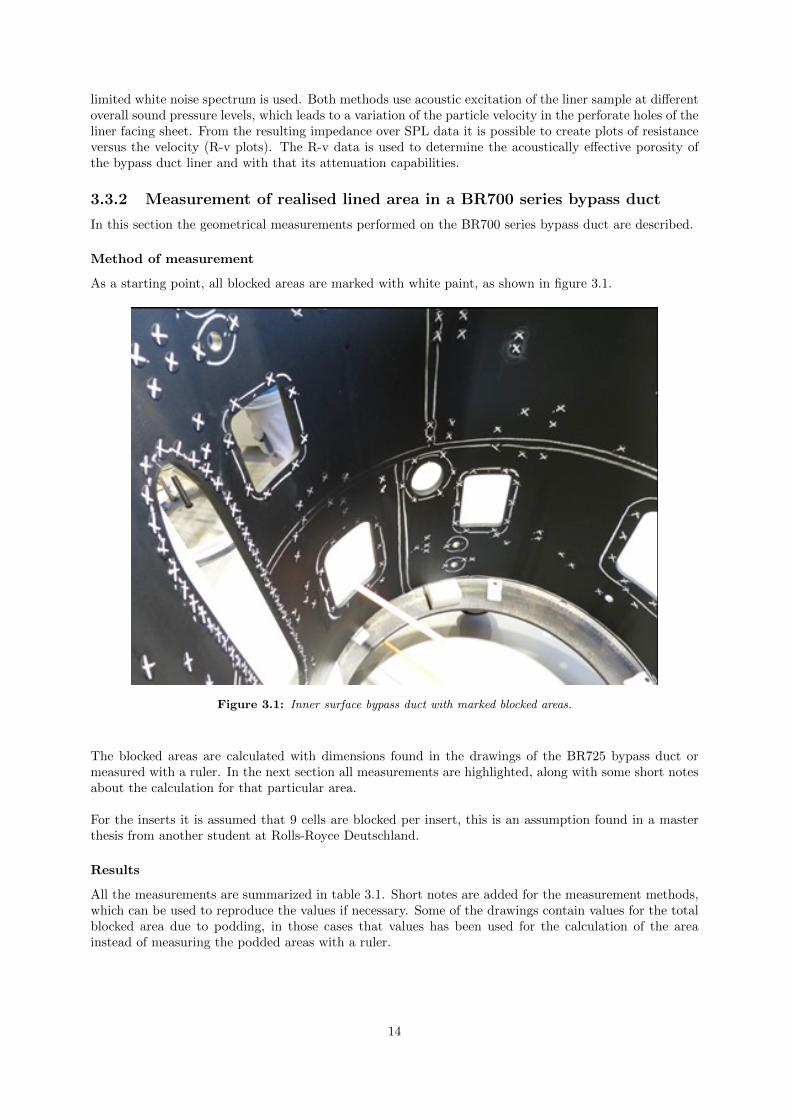
As a starting point, all blocked areas are marked with white paint, as shown in figure 3.1.

Figure 3.1: Inner surface bypass duct with marked blocked areas.

The blocked areas are calculated with dimensions found in the drawings of the BR725 bypass duct ormeasured with a ruler. In the next section all measurements are highlighted, along with some short notesabout the calculation for that particular area.

For the inserts it is assumed that 9 cells are blocked per insert, this is an assumption found in a masterthesis from another student at Rolls-Royce Deutschland.

Results

All the measurements are summarized in table 3.1. Short notes are added for the measurement methods,which can be used to reproduce the values if necessary. Some of the drawings contain values for the totalblocked area due to podding, in those cases that values has been used for the calculation of the areainstead of measuring the podded areas with a ruler.

14

Blocked area (Percent-age of total cone area)

Notes

Rear flange podded cells 0.79% Diameter from drawing, width withruler (average of 4 points)

Central circumferential hon-eycomb split line blockedcells

1.40% Average diameter, from top and bot-tom circumference, height same as topcircumference

Front flange podded cells 0.75% Same as top circumferenceFacing sheet split lines (6x) 1.48% Height of a cone via online calculator,

subtracted height of circumferences,values divided by two since the lines arenot present at the whole height, widthwith a ruler

Honeycomb split line vertical(4x)

0.27% Width with ruler, minus values of cross-ing panels

Honeycomb split line hori-zontal

0.24% Average diameter at 1/5 of height,minus values of crossing panels

Drainage Hole 0.00% Diameter with a ruler, not present onthe drawings

Service fairing and surround-ing podded area

2.70% Assumed squares according to lengthon drawing, plus half circles accordingto radius from drawing

BCO- holes (8x) 0.71% Average diameter at two pointsAir- cooler 7.33% No drawing, square and three circular

surfacesAccess panel big (4x) 6.91% Measured two squares, full circle for

the corners, average for two points hori-zontal and vertical, plus 30 mm for thesurrounding circle (to account for vis-ible podding around the access panel)

Access panel medium (4x) 4.25% Same as big access panelAccess panel small (2x) 1.62% Same as big access panelAccess panel circular (2x) 1.17% Diameter from drawingPodded Inserts 4.87% 9 blocked cells, per insert, size per

blocked cell calculated from a drawingwhich describes distances between cells

Total bypass duct surface 100% Top and bottom diameter, real sidelength from a cone according to onlinecalculator

Table 3.1: Blocked areas and total bypass duct surface.

Reviewing results

The results of this assessment are compared to the results of an old assessment in 2009. The old assessmentincludes 10% blockage by paint, where that part is excluded here and is accounted for in the impedancepart.

Subtracting the blocked area from the total bypass duct surface results in the acoustic lined area for thisassessment. The current model is based on the old assessment of 2009. Here, the old model without paintblockage means that the 10% is included as acoustic lined area and with paint blockage means that 10%from the old value of the acoustic lined area is subtracted (and thus assumed as totally blocking).

The new measurements show a decrease of 3.05% in acoustic lined area, or an increase of 7.63% withincluding blockage due to paint in the old/current model.

15

The measurements are summarised in the charts in figure3.2 and 3.3. The biggest differences are foundin the inserts, where more area is blocked since all inserts are assumed to be podded (which leads tomore blockage of acoustic lined area). Next to that, the splitter cut-out also shows a big change whichreduces the blocked area. The origin of that change could not be identified, and it is assumed to be anapproximation error in the assessment of the relatively complex geometry of the service faring.

It must be noted, that the discrepancy found in the current assessment does not reflect a change relativeto the production standard used during noise certification tests, but indicates the modelling uncertainty,that is intended to be removed for an improved reproduction of the bypass duct liner in the acoustic linermodel.

Figure 3.2: Percentages of acoustic liner and blocked area, old (current model).

Figure 3.3: Percentages of acoustic liner and blocked area, new.

16

3.3.3 Impedance measurements at BR700 series bypass duct

To include for blockage by paint in the acoustic liner model, impedance measurements are carried out.The measurement system used for the non-destructive impedance measurement is a B&K WA1599 typeimpedance tube. Measuring the acoustic impedance of a surface gives a complex representation of itsacoustic resistance and reactance. The diameter of the measurement section is 29mm. Repeated meas-urements of the acoustic impedance at various measurement positions along acoustically active surface ofthe bypass duct liner provides a representation of the average impedance as well as the variation of theimpedance. Furthermore, the measurements with increasing SPL provide R-v characteristics, which areused to calculate the effective acoustic porosity of the liner facing sheet. Various points inside the bypassduct are measured to review the acoustical behaviour of the bypass duct and to check for any variation.

Method of measurements

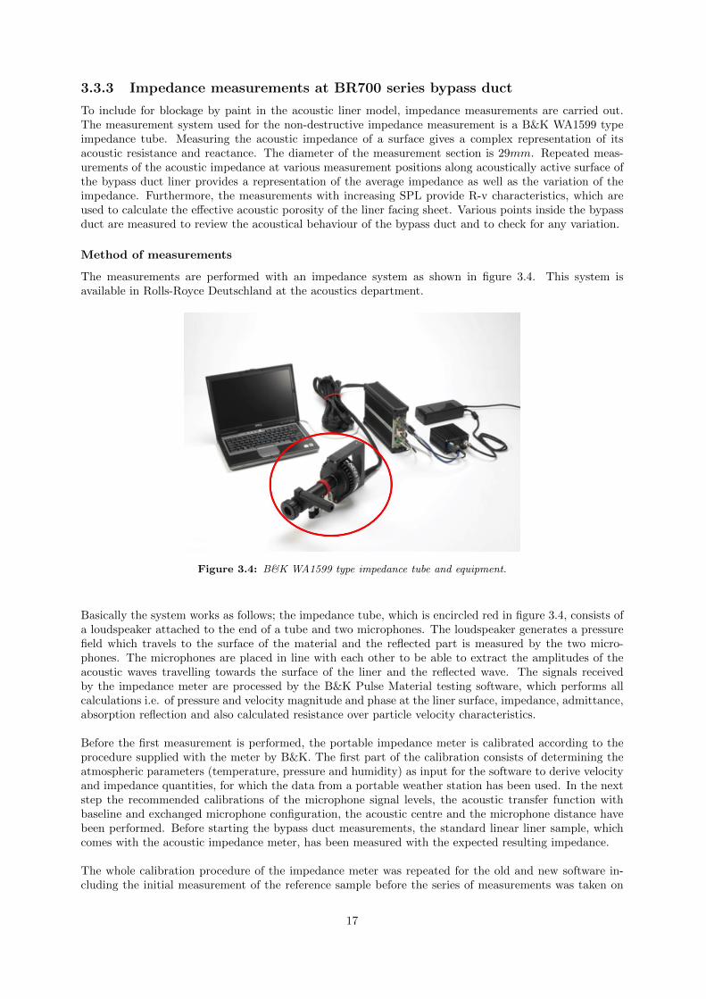
The measurements are performed with an impedance system as shown in figure 3.4. This system isavailable in Rolls-Royce Deutschland at the acoustics department.

Figure 3.4: B&K WA1599 type impedance tube and equipment.

Basically the system works as follows; the impedance tube, which is encircled red in figure 3.4, consists ofa loudspeaker attached to the end of a tube and two microphones. The loudspeaker generates a pressurefield which travels to the surface of the material and the reflected part is measured by the two micro-phones. The microphones are placed in line with each other to be able to extract the amplitudes of theacoustic waves travelling towards the surface of the liner and the reflected wave. The signals receivedby the impedance meter are processed by the B&K Pulse Material testing software, which performs allcalculations i.e. of pressure and velocity magnitude and phase at the liner surface, impedance, admittance,absorption reflection and also calculated resistance over particle velocity characteristics.

Before the first measurement is performed, the portable impedance meter is calibrated according to theprocedure supplied with the meter by B&K. The first part of the calibration consists of determining theatmospheric parameters (temperature, pressure and humidity) as input for the software to derive velocityand impedance quantities, for which the data from a portable weather station has been used. In the nextstep the recommended calibrations of the microphone signal levels, the acoustic transfer function withbaseline and exchanged microphone configuration, the acoustic centre and the microphone distance havebeen performed. Before starting the bypass duct measurements, the standard linear liner sample, whichcomes with the acoustic impedance meter, has been measured with the expected resulting impedance.

The whole calibration procedure of the impedance meter was repeated for the old and new software in-cluding the initial measurement of the reference sample before the series of measurements was taken on

17

the bypass duct liner. During the calibration there were no abnormal findings.

For this assessment, two different software systems are used with two different measurements methods.

• The first series of measurements is performed with Pulse software version 16 and a single frequencySPL loop for 10 points along the TDC (Top Death Centre) line. Those measurements are referredto as the line measurements.

• The second series of measurements is performed with Pulse software version 18, which is capableof a BB SPL loop. This is done for 4 circles at different heights along the bypass duct where eachcircle consists of 10 points. Those measurements are referred to as the circular measurements. Thecircles cross the line measurement at about the 4th to 6th measurement point for each circle.

In total 50 points inside the bypass duct are examined with the portable impedance meter. As mentionedbefore, all points are not in the near vicinity of any of the fairings, panels or other disturbed areas. Specialattention is paid to cover the observed variety of very open and closed regions within the bypass ductacoustic lined area. Open means low visible blockage of apertures and closed means that multiple aper-tures in the measurement area show visible blockage. This gives a clear view of the variety of the porosityopen area of the liner, which is explained later on.

The data gathered by the software is exported to excel for further data analysis. Unfortunately, the newsoftware had some problems exporting the data and failed to export everything. In the end, it seems thatthe amount of data for the BB SPL loop was much bigger than for the SPL loop, since the BB SPL loopcontains more sound levels and data points which caused problems exporting. Splitting the export processup in parts fixed this issue eventually, which made all data usable.

Results, d-POA and porosity graphs

One part of the exported data consists of non-dimensional acoustic resistance versus velocity data, whichcan be used to determine the effective hole diameter and the effective porosity open area. The data isavailable for different sound levels, usually from 128dB to 146dB with a step size of 6dB. Typical soundlevels found in an aero engine during noise certification flight are within the top end of this range but canalso exceed these values. Sometimes extrapolated and interpolated values are also present, all extrapolatedvalues are excluded from the analysis of the R-v slope and the effective acoustic porosity.

The specified and made geometrical parameters of the liner are given below. They are controlled i.e.using pins of nominal, maximum and minimum size and by measuring the aperture spacing during theproduction process. The first value describes the hole diameter and the second value the porosity openarea of the liner including their tolerances. The values are symbolic and only the tolerances are given forpublicity reasons.

dtheor = d± 0.05mm

POAtheor = POA± 1%

As the fully assembled liner panel with paint shows blockage of holes and any kind of variation due tobonding material remains and paint, an acoustical analysis of the liner is desired. This is performed withthe portable impedance meter and the result is used to calculate the acoustically effective geometry of theliner. This effective geometry is expected to deviate from the above nominal values.

The B&K materials testing module uses the atmospheric parameters in various internal calculations. Fur-thermore, the calculation of the effective acoustic porosity also requires the atmospheric parameters; thespeed of sound (c), as well as the theoretical hole pitch and the cavity discharge coefficient (which is anempirically derived model parameter).

18

The atmospheric parameters, which are determined by a portable weather station:

Temperature; T = 22°CPressure; P = 100700Pa

Relative humidity; = 33%

And thereof the speed of sound is derived:

c =√γRT = 344.40m/s

Where;

γ = 1.4

R = 287.05J

Kg ·KT = 273 + 22 = 295K

Furthermore, geometrical parameters of the panel are required. It is assumed, that the hole pitch is wellcontrolled in the production process and if at all only subject to stochastic, but not systematic ,variation.The theoretical hole pitch is calculated from the hole diameter and porosity for the square hole patternof the bypass duct liner to be p = 3.5035mm and a cavity discharge coefficient for a classical perforate liner.

From the measured resistance versus velocity data, both the slope and interception points are derived.The slope is used to calculate the effective porosity open area.

Combining the slope with the interception point, line graphs (R-v graphs) can be produced. Those linegraphs are used as a sanity check to exclude any misleading measurements. For example, the 7th pointfor one of the circular measurements is excluded since the graph is not close to linear, this is shown belowin figure 3.5. It is clear that the points are not in line, possible due to movement of the impedance meterduring the measurement.

Figure 3.5: Resistance vs. velocity, 7th point of a circular measurement at the rear end of the bypass duct.

Also, the effective hole diameter is calculated according to a specific ratio of the effective porosity openarea. The effective porosity open area, effective hole diameter and a histogram showing the variety of theporosity can be found in the appendix (figure 6.1, 6.2 and 6.3). All charts show that the line measurementsthat are performed along the TDC line show slightly lower values than the circular measurements and alsoless variation around the average values. They also show that the average values for the line measurements

19

are indeed below the theoretical values and the circular measurements show average values far above themaximum variation for the theoretical values.

In the appendix table 6.1 the charts are summarized and indicate that the circular measurements are notwithin the prescribed tolerances. However, the discrepancy between the circular and the line measurementslead to further investigation of the circular measurements with the new software version and BB excitation.

The line measurements show reasonable values, which are slightly lower than the theoretical values. Thisis expected since the paint partially blocks the holes, resulting in a reduced porosity and hole diameter.

In all charts, one sample point is clearly showing an invalid measurement. In the next section this pointis excluded from the measurements and also the circular measurements are investigated.

Correction of wrong environment setting in the new software

In a further investigation of the measurement properties of the circular measurements a wrong settingof the atmospheric parameters was found. The cause was that Pulse software version 18 was configuredto use an environmental sensor, which was not present in the Rolls-Royce Impedance meter hardware.Therefore, wrong base values instead of the correct values from the weather station were used for thesoftware internal calculations, which are:

Temperature; T = −2.94°CPressure; P = 78620Pa

Relative humidity; = 0%

Therefore, the commissioning of the new software was considered unsuccessful and the old software is usedfurther until an update becomes available for the new software version.

The wrong atmospheric settings would result in a different value for the speed of sound and density. Thepossible errors are checked by scaling the resistance and velocity data with different values for the speedof sound and density against the initial values for those parameters of the program.

The wrong values used in the internal calculations of the Pulse software are:

Speed of sound; c = 329.53m/s

Density of air; ρ = 1.012kg/m3

These have to be scaled to the following correct readings from the weather station:

Speed of sound; c = 344.40m/s

Density of air; ρ = 1.189kg/m3

Where;

ρ = p/RT

The following density and speed of sound scaling is applied to the resistance and velocity data:

Resistance; R = Rmeasured · (1.889/1.012) · (344.4/329.53)

Velocity; v = vmeasured · (1.012/1.889) · (329.53/344.4)

20

The scaling formulas show that the resistance increases with increasing specific impedance of air (speedof sound times density) and the velocity decreases, which is reasonable for a higher temperature than initial.

The results after scaling are summarized in table 6.2 in the appendix.

Excluding the invalid measurement found in the previous section reduces the error even more. This pointis referred to as C-Rear 7, which is the 7th measurement of a circular measurement performed at the readend of the bypass duct. The final results after scaling and excluding C-Rear 7 are shown in table 3.2.

Values Difference relativeto theoretical

Within tolerance

d theoretical dmm Tolerance = 0.05mmd average circular −mm 0.91% Yesd average TDCline −mm −0.83% Yes

POA theoretical POA% Tolerance = 1%POA average circular −% 2.13% YesPOA average TDCline −% −1.43% Yes

Table 3.2: Theoretical, average hole diameter and porosity values after scaling and excluding C-Rear 7.

As can be concluded from the tables above, the values of both subsequent measurements with differentsoftware and excitation form are now close to each other and close to the theoretical values and within thespecified tolerance. The hole diameter, porosity and histogram charts are shown in the following figuresand also show a more reasonable distribution around the theoretical values. After the scaling process, thecircular measurements are considered as valid again and used for further analysis.

The final results are shown in the following figures. In all figures one of the axes is left out. The histogramin figure 3.9 is used to update the noise model for impedance variation.

Figure 3.6: Effective hole diameter, scaled.

21

Figure 3.7: Effective porosity, scaled.

Figure 3.8: POA vs. hole diameter, scaled.

22

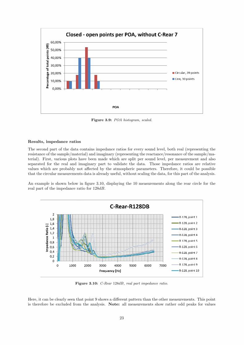
Figure 3.9: POA histogram, scaled.

Results, impedance ratios

The second part of the data contains impedance ratios for every sound level, both real (representing theresistance of the sample/material) and imaginary (representing the reactance/resonance of the sample/ma-terial). First, various plots have been made which are split per sound level, per measurement and alsoseparated for the real and imaginary part to validate the data. Those impedance ratios are relativevalues which are probably not affected by the atmospheric parameters. Therefore, it could be possiblethat the circular measurements data is already useful, without scaling the data, for this part of the analysis.

An example is shown below in figure 3.10, displaying the 10 measurements along the rear circle for thereal part of the impedance ratio for 128dB.

Figure 3.10: C-Rear 128dB, real part impedance ratio.

Here, it can be clearly seen that point 9 shows a different pattern than the other measurements. This pointis therefore be excluded from the analysis. Note: all measurements show rather odd peaks for values

23

lower than 3000Hz. Unfortunately, those peaks are unexplainable but also irrelevant for this analysissince they are not within the range which is analysed in this assessment.

In the appendix, figure 6.1, 6.2 and 6.3, combined charts for every sound level are shown, displaying thevariety for all measurements. Each plot shows clearly that most of the measurements show the samepattern and therefore the total set of measurements could be considered as usable/valid.

In the next step all the impedance ratios for the different sound levels are averaged for each sound leveland represented in one chart along with the predictions made in vu20 (liner prediction and optimisationtoolbox) based on the derived average values for the hole diameter and porosity open area for both lineand circular measurements. The predictions based on the uncorrected average hole diameter and porosityfor the circular measurements can be found in the appendix, since they are not representative. Here, itis not possible, as expected, to scale the impedance ratios to the circular predictions. Using the updatedvalues for the averages results in nearly the same predictions as used in the line predictions and are thusleft out for convenience.

For the real impedance plot the only point of interest is around 2.8kHz, mainly for two reasons:

• Range of the impedance meter; 500Hz − 6.3kHz. Below this range the microphone spacing causeserrors in the data and above this range it is not possible to have only plane waves, since certainmode shapes start to occur.

• Sample frequency, of 2.8kHz. This is the only reliable point, representing the lowest resistance value.Empirical results show that the higher resistance values are more easily affected by environmentalparameters. Next to that, the sample frequency is well within the range of the impedance meter.

In figure 3.11 and 3.12 both prediction plots are displayed. For the real plot it is clear that the predictedvalues are close to the measured values around the sample frequency and for the imaginary plot the slopeand zero crossing of the prediction fits the measurements very well. Both charts conclude that the currentmodel is close to reality.

Figure 3.11: Average impedance ratios per sound level with predictions, real part.

24

Figure 3.12: Average impedance ratios per sound level with predictions, imaginary part.

Note: for the imaginary plot an area ratio is used to create a better fit for the data. This area ratioaccounts for discontinuities in the flow due to the sudden area jump between the impedance tube andthe effective area underneath inside the liner formed by the honeycomb cells (not all cells perfectly fit theedge of the tube).

25

Conclusion

In total the assessment of the current production standard BR700 series bypass duct liner by most recentmodelling and measurement methods has identified modelling discrepancies that result in a change in thepredicted total aircraft noise in the range of 0.13 and 0.16∆EPNdB depending on variation of POA alongthe bypass duct.

This change is combined of an uncertainty between the modelled and achieved acoustically active area inthe bypass duct and the impedance of the painted SDOF liner in the bypass duct main structure.

During the assessment it was found, that the assumption of total blockage by paint from a previous as-sessment of the bypass duct was too conservative and that in fact, the blocked area by paint and also bythe service fairing cut-out is smaller than assumed before. However, it was also found, that more area isblocked by podded inserts than previously assumed, ending up in a total increase of the lined area in thebypass duct by about 6%, which corresponds to an additional predicted noise reduction of 0.09∆EPNdB.

The impedance measurements with the painted bypass duct confirmed, that the specified impedance isvery well met by the painted bypass duct and that the paint blockage does not significantly change imped-ance. The corresponding modelling improvement leads to an additional noise reduction of 0.02∆EPNdB.

Finally the observed variation is assessed by splitting the bypass duct into sections with different POAand hole diameter according to the result of the acoustic measurements. Even though the two subsets(40 circular along half circles in a single axial position and 10 measurements along the TDC line) aftercorrections are applied are only slightly different, the resulting 0.03∆EPNdB between the two almostidentical measurements indicate a relative large impact of the variation relative to other changes discussedbefore.

Most of the current findings correspond to modelling improvements and lead to removing conservatismto account for paint blockage. In consequence, the most likely result of removing the paint will be nomeasurable change on noise.

To summarise, removing the paint will not have a significant noise benefit relative to the current statusof the painted BR700 series bypass duct. This is because the achieved acoustic properties of the currentbypass duct are close to the specifications of the unpainted bypass duct. However, it is expected, that thevariation of porosity along the bypass duct would be reduced by removing the paint along with cost andweight benefits.

26

4 Assignment 3: Weather data analysis forengine noise testing

4.1 Assignment description

The third assignment consists of a weather study for an engine test bed in Stennis. This test bed is usedto perform noise tests for different engine types, the test bed is shown in figure 4.1.

Figure 4.1: Test bed Stennis.

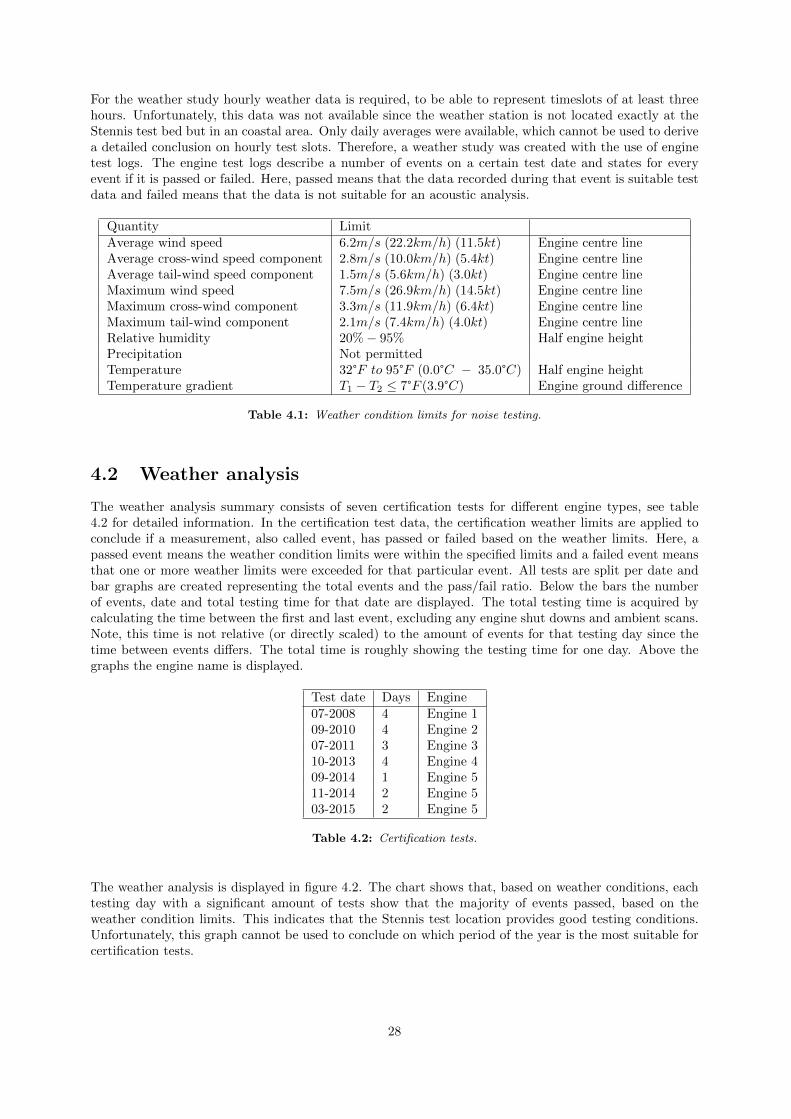
The test bed is used to perform both certification and development tests, where certification tests areused to prove that a certain engine is able to operate within the specified noise limits. A customer ofRolls-Royce asked for a weather study, which shows that the Stennis test bed is capable of performingengine certification tests for at least three hours without breaks. The test bed is considered suitable asif the weather conditions are within certain specified limits, those limits are shown in table 4.11. Note,the weather condition limits are stated within Rolls-Royce Deutschland test reports for engine testingbut are also publicly available. The weather conditions are monitored with a meteorological measurementsystem to ensure that static noise tests are conducted within specific meteorological limits and to provideinformation needed for acoustical data normalisation to reference meteorological conditions.

1SAE ARP1846A Issued 1990-02, Revised 2008-03

27

For the weather study hourly weather data is required, to be able to represent timeslots of at least threehours. Unfortunately, this data was not available since the weather station is not located exactly at theStennis test bed but in an coastal area. Only daily averages were available, which cannot be used to derivea detailed conclusion on hourly test slots. Therefore, a weather study was created with the use of enginetest logs. The engine test logs describe a number of events on a certain test date and states for everyevent if it is passed or failed. Here, passed means that the data recorded during that event is suitable testdata and failed means that the data is not suitable for an acoustic analysis.

Quantity LimitAverage wind speed 6.2m/s (22.2km/h) (11.5kt) Engine centre lineAverage cross-wind speed component 2.8m/s (10.0km/h) (5.4kt) Engine centre lineAverage tail-wind speed component 1.5m/s (5.6km/h) (3.0kt) Engine centre lineMaximum wind speed 7.5m/s (26.9km/h) (14.5kt) Engine centre lineMaximum cross-wind component 3.3m/s (11.9km/h) (6.4kt) Engine centre lineMaximum tail-wind component 2.1m/s (7.4km/h) (4.0kt) Engine centre lineRelative humidity 20% − 95% Half engine heightPrecipitation Not permittedTemperature 32°F to 95°F (0.0°C − 35.0°C) Half engine heightTemperature gradient T1 − T2 ≤ 7°F (3.9°C) Engine ground difference

Table 4.1: Weather condition limits for noise testing.

4.2 Weather analysis

The weather analysis summary consists of seven certification tests for different engine types, see table4.2 for detailed information. In the certification test data, the certification weather limits are applied toconclude if a measurement, also called event, has passed or failed based on the weather limits. Here, apassed event means the weather condition limits were within the specified limits and a failed event meansthat one or more weather limits were exceeded for that particular event. All tests are split per date andbar graphs are created representing the total events and the pass/fail ratio. Below the bars the numberof events, date and total testing time for that date are displayed. The total testing time is acquired bycalculating the time between the first and last event, excluding any engine shut downs and ambient scans.Note, this time is not relative (or directly scaled) to the amount of events for that testing day since thetime between events differs. The total time is roughly showing the testing time for one day. Above thegraphs the engine name is displayed.

Test date Days Engine07-2008 4 Engine 109-2010 4 Engine 207-2011 3 Engine 310-2013 4 Engine 409-2014 1 Engine 511-2014 2 Engine 503-2015 2 Engine 5

Table 4.2: Certification tests.

The weather analysis is displayed in figure 4.2. The chart shows that, based on weather conditions, eachtesting day with a significant amount of tests show that the majority of events passed, based on theweather condition limits. This indicates that the Stennis test location provides good testing conditions.Unfortunately, this graph cannot be used to conclude on which period of the year is the most suitable forcertification tests.

28

Figure

4.2:

Wea

ther

stu

dy

Ste

nn

is.

29

5 Reflection

In this chapter a short reflection is given on my internship at Rolls-Royce Deutschland.

My first assignment mainly consists of code developing within Matlab. Hereby, I greatly improved myMatlab programming skills and I am now able to construct a code in a structured and organised way. Thisassignment clearly showed me the power of Matlab within an engineering department. Writing a codewith a graphical user interface was completely new to me and I also learned a new way of code debuggingwithin complex codes. I think the improvement in Matlab code developing together with designing thevalidation sheet and user and developer documentation is a valuable addition in the current engineeringenvironment. Lastly, creating a test log clearly showed the importance of code testing in order to debugerrors which are not shown directly by Matlab.

The other assignments gave a nice overview of all kind of assessments which occur in a working envir-onment. Within the second assignment I gained knowledge about acoustic liner calculations, performingacoustic liner measurements with complicated tools and writing detailed documentation. For the secondassignment I also attended a Foreign Object Damage training, to minimise casualties during the measure-ments. The third assignment was a rather minor task but clearly showed the importance and limitationsof weather conditions for engine testing.

Usually, many students perform one assignment during there internship but in my opinion a combinationof different assignments gives a broad overview of all kind of engineering tasks within a specific departmentand in gaining practical experience. In this way, I really felt as a valuable addition to the department,especially since many of the tasks are performed within a team combined with regular meetings which Ithink is a great addition to the experience of a starting engineer.

To summarise, below a list of skills and personal findings acquired during this internship is shown.

• Deepening Matlab skills, especially:

– GUI handling.

– Version control software for software development.

– Detailed documentation.

– Comprehensive tool testing and logging.

• Acoustic impedance testing including test preparation, performing measurements and data analysis.

• Performing in a large open-plan company and to perform in a team.

Overall, the internship at Rolls-Royce Deutschland was a great contribution to my study Mechanical En-gineering and I would highly recommend RRD to other students, especially the Aeroacoustics and Noisedepartment.

Niek van Dijk

30

6 Appendix

The appendix contains figures and tables related to the second assignment.

Figure 6.1 and 6.2 show the uncorrected hole diameter and porosity, this data is directly taken from themeasurements. It is clear that the average values for the circular measurements are not within the specifiedtolerance (see table 6.1 for more details). A combined chart is shown in figure 6.3. Table 6.2 shows thescaled results but including C-Rear 7.

Figure 6.1: Effective hole diameter, uncorrected.

Figure 6.2: Effective porosity, uncorrected.

31

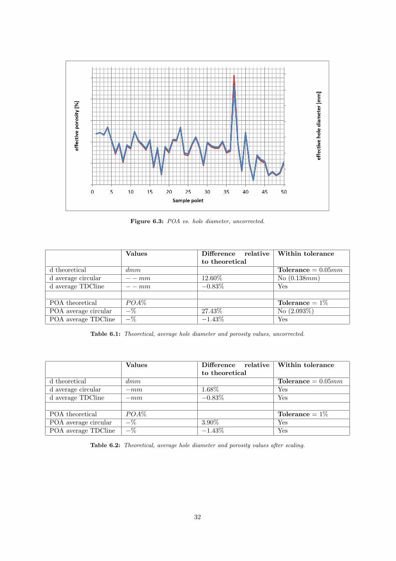
Figure 6.3: POA vs. hole diameter, uncorrected.

Values Difference relativeto theoretical

Within tolerance

d theoretical dmm Tolerance = 0.05mmd average circular −−mm 12.60% No (0.138mm)d average TDCline −−mm −0.83% Yes

POA theoretical POA% Tolerance = 1%POA average circular −% 27.43% No (2.093%)POA average TDCline −% −1.43% Yes

Table 6.1: Theoretical, average hole diameter and porosity values, uncorrected.

Values Difference relativeto theoretical

Within tolerance

d theoretical dmm Tolerance = 0.05mmd average circular −mm 1.68% Yesd average TDCline −mm −0.83% Yes

POA theoretical POA% Tolerance = 1%POA average circular −% 3.90% YesPOA average TDCline −% −1.43% Yes

Table 6.2: Theoretical, average hole diameter and porosity values after scaling.

32