Embed Size (px)
Citation preview

EUROPEAN RAILWAY AGENCY
PAGE 1 OF 64
INTEROPERABILITY UNIT
RUNNING DYNAMICS
APPLICATION OF EN 14363:2005 – MODIFICATIONS AND CLARIFICATIONS
REFERENCE: ERA/TD/2012-17/INT DOCUMENT TYPE:
TECHNICAL DOCUMENT
VERSION: 3.0
DATE: 17/12/2014
Edited by Reviewed by Approved by
Name Mikael AHO
Hubert LAVOGIEZ Denis BIASIN
Position Project Officer Head of Sector Head of Interoperability Unit
Date
&
Signat.
18/06/2013 18/06/2013 18/06/2013
European Railway Agency
Rolling Stock - Subsystem
Version 3.0 Page 2/64
AMENDMENT RECORD
Version Date Section number
Modification/description Author
1.0 16/11/2012 Final draft Mikael AHO
2.0 18/06/2013 Editorial modifications, references corrected.
Document presented to RISC 67 on 06 June 2013.
Mikael AHO
3.0 17/12/2014 Editorial modifications, references corrected and
mistakes corrected.
Pedro MESTRE
European Railway Agency
Rolling Stock - Subsystem
Version 3.0 Page 3/64
Table of Contents
1. Introduction ........................................................................................... 6
2. Abbreviations and references ..................................................................... 7
2.1 Abbreviations ................................................................................. 7
2.2 References .................................................................................... 7
3. Purpose of the document .......................................................................... 9
4. Application of EN 14363:2005 and the modifications of it ................................... 10
4.1 Fundamental understanding for the application of EN 14363 ........................ 10
4.2 Terms and definitions ....................................................................... 11
4.2.1 Target test conditions ..................................................................11
4.2.2 Reference conditions ..................................................................11
4.2.3 Bogie yaw resistance ..................................................................11
4.2.4 Unsprung mass .........................................................................11
4.2.5 Primary suspended mass .............................................................11
4.2.6 Secondary suspended mass .........................................................12
4.2.7 Bogie mass ..............................................................................12
4.2.8 Yaw moment of inertia of whole running gear .....................................12
4.2.9 Running behaviour .....................................................................12
4.2.10 Equivalent conicity ...................................................................12
4.2.11 Operation envelope .................................................................12
4.2.12 Conventional technology vehicle ..................................................12
4.2.13 Reference vehicle ...................................................................13
4.2.14 Engineering change .................................................................13
4.2.15 Validation report .....................................................................13
4.2.16 Simulation report .....................................................................13
4.3 Modified conditions ......................................................................... 14
4.3.1 Loading conditions .....................................................................14
4.3.2 Safety against derailment on twisted track .........................................14
4.3.3 Requirements for assessment of fault modes .....................................15
4.3.4 Track quality ............................................................................16
4.3.5 Stability testing .........................................................................19
4.3.6 Contact Conditions .....................................................................19
4.3.7 Target cant deficiency for the evaluation of quasistatic assessment quantities
...........................................................................................20
European Railway Agency
Rolling Stock - Subsystem
Version 3.0 Page 4/64
4.3.8 Test speed for vehicles with Vadm>300 km/h .....................................20
4.3.9 Multiple regression against target test conditions .................................20
4.3.10 Alternative evaluation for Y/Q .....................................................21
4.3.11 Evaluation of quasistatic guiding force Yqst ......................................21
4.3.12 Evaluation of additional track loading parameters..............................22
4.4 Methods to assess the vehicle against missing target test conditions .............. 22
4.4.1 Operating envelope ....................................................................22
4.4.2 Track section length Lts ................................................................22
4.4.3 Minimal number of track sections nts,min in test zone 3 ...........................22
4.4.4 Minimal total length of track sections Lts,min in test zone 2 ......................22
4.4.5 Methodology, when the minimum number of sections nts,min is not fulfilled in a
test zone ...........................................................................................22
4.4.6 Improve relevance of estimated value in 2-dimensional evaluation ............24
4.4.7 Use of simulation to complement investigations for a proper assessment....24
4.4.8 Multiple regressions against target test conditions ...............................25
4.4.9 Extension of acceptance / Instrumentation of trainsets ..........................25
ANNEX A DETERMINATION OF ESTIMATED VALUES USING MULTI LINEAR EVALUATION ......... 26
A.1 Technical and statistical theory ................................................... 26
A.2 Test conditions – allowed ranges for the evaluation ....................... 26
A.3 Specified process for the correction of estimated values ................. 28
A.4 Specified process for multi linear determination of estimated values 29
A.5 Documentation ......................................................................... 31
ANNEX B SIMULATION ................................................................................. 32
B.1 Introduction .............................................................................. 32
B.2 Scope ...................................................................................... 32
B.2.1 General .................................................................................32
B.2.2 Extension of the range of test conditions ...................................32
B.2.3 Verification of vehicle dynamic behaviour following modification ...33
B.2.4 Verification of new vehicles dynamic behaviour by comparison with
an already approved Reference Vehicle ................................................33
B 2.5 Investigation of dynamic behaviour in case of fault modes ...........34
B.3 Validation ..................................................................................... 35
B.3.1 General principles ...................................................................35
B.3.2 Vehicle model .........................................................................35
B.3.3 Validation of the vehicle model .................................................35

European Railway Agency
Rolling Stock - Subsystem
Version 3.0 Page 5/64
B.4 Input ....................................................................................... 43
B.4.1 Introduction ...........................................................................43
B.4.2 Vehicle model .........................................................................44
B.4.3 Vehicle configuration ...............................................................44
B.4.4 Track data .............................................................................44
B.4.5 Track model parameters ..........................................................45
B.4.6 Wheel-rail contact geometry ....................................................46
B.4.7 Rail surface condition ..............................................................46
B.4.8 Direction of travel ...................................................................46
B.4.9 Speed ...................................................................................47
B.4.10 Position of the vehicle in the trainset .........................................47
B.4.11 Frequency content of simulations ..........................................47
B.5 Output ..................................................................................... 48
B.5.1 Methods to determine the estimated value from the simulation ....48
B.6 Report ..................................................................................... 49
B.7 Examples for model validation (recommended only) ...................... 49
ANNEX C EXTENSION OF APPROVAL .................................................................. 54
C.1 General .................................................................................... 54
C.2 Determination of the safety factor ............................................. 59
C.3 Dispensation ............................................................................. 59
C.3.1 General .................................................................................59
C.3.2 Special cases ..........................................................................59
C.4 Check for base conditions for Simplified Method ............................ 60
C.5 Requirements depending on the initial approval ............................ 60
ANNEX D EVALUATION OF CONTACT GEOMETRY PARAMETERS ..................................... 62
D.1 Evaluation of equivalent conicity ................................................. 62
D.2 Requirements for manual rail profile measurements ...................... 62
D.2.1 General ...............................................................................62
D.2.2 Measurements for equivalent conicity .....................................62
D.2.3 Automatic measurements ......................................................63

European Railway Agency
Rolling Stock - Subsystem
Version 3.0 Page 6/64
1. Introduction
The present document provides the necessary additional specifications to
perform running dynamic behaviour testing of rolling stock.
Reference is made to this document as mandatory specification in clause 4.2.3.4
(and Annex J.2) of the revision of the TSI LOC&PAS, entering into force on
01/01/2015.
European Railway Agency
Rolling Stock - Subsystem
Version 3.0 Page 7/64
2. Abbreviations and references
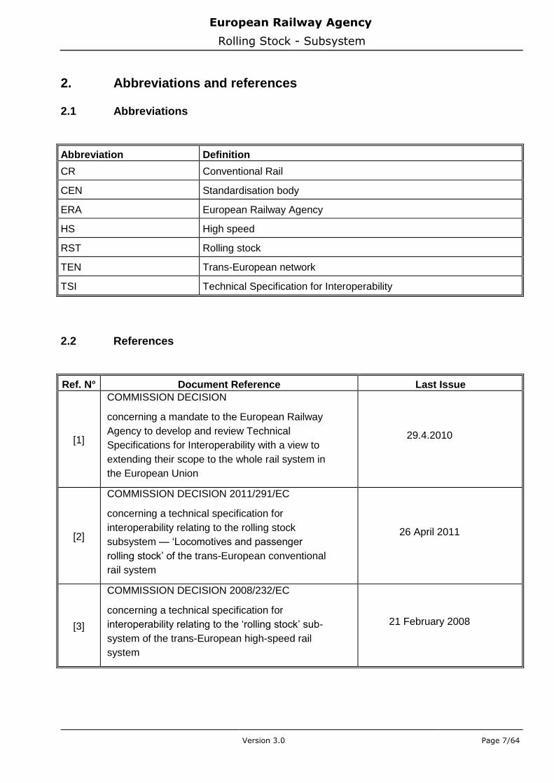
2.1 Abbreviations
Abbreviation Definition
CR Conventional Rail
CEN Standardisation body
ERA European Railway Agency
HS High speed
RST Rolling stock
TEN Trans-European network
TSI Technical Specification for Interoperability
2.2 References
Ref. N° Document Reference Last Issue
[1]
COMMISSION DECISION
concerning a mandate to the European Railway
Agency to develop and review Technical
Specifications for Interoperability with a view to
extending their scope to the whole rail system in
the European Union
29.4.2010
[2]
COMMISSION DECISION 2011/291/EC
concerning a technical specification for
interoperability relating to the rolling stock
subsystem — ‘Locomotives and passenger
rolling stock’ of the trans-European conventional
rail system
26 April 2011
[3]
COMMISSION DECISION 2008/232/EC
concerning a technical specification for
interoperability relating to the ‘rolling stock’ sub-
system of the trans-European high-speed rail
system
21 February 2008

European Railway Agency
Rolling Stock - Subsystem
Version 3.0 Page 8/64
Ref. N° Document Reference Last Issue
[4]
DIRECTIVE 2008/57/EC OF THE EUROPEAN
PARLIAMENT AND OF THE COUNCIL
on the interoperability of the rail system within
the Community
17 June 2008

European Railway Agency
Rolling Stock - Subsystem
Version 3.0 Page 9/64
3. Purpose of the document
The Commission has in the mandate [1] commissioned the Agency to revise the RST TSIs
[2] and [3] particularly in respect of closing open points identified in the two TSIs.
The running dynamic behaviour test conditions in regard of track geometric quality and the
combination of speed, curvature and cant deficiency are open points in the CR LOC&PAS
RST TSI [2] and HS RST TSI [3].
These open points are subject to work involving CEN WGs on rolling stock testing and
infrastructure maintenance specifications.
The Agency has launched a WP to specifically address the open points in the RST TSIs.
In the WP it has been decided that CEN WG work is taken over in a technical document
(the present document) pre-empting the publication of the appropriate standard revisions,
at which point the TSI will refer to them and this Technical document will be withdrawn by
a revision procedure as set out in the Directive [4].
In the following sections of this document the conditions, methods and track geometric
quality for the running dynamic behavior testing are outlined for assessing a rolling stock
running dynamic behaviour under the TSI LOC&PAS.

European Railway Agency
Rolling Stock - Subsystem
Version 3.0 Page 10/64
4. Application of EN 14363:2005 and the modifications of it
4.1 Fundamental understanding for the application of EN 14363
In the open point of the RST TSIs it is recognised that for practical reasons not all of the
target test conditions identified in EN 14363 are achievable by physical testing.
If the combination of all target test conditions is not completely achievable, compliance
shall be demonstrated by assessing the vehicle against some missing target test
conditions of EN 14363:2005 also by other means than described in EN 14363:2005.
This document gives examples of methods for the case that the combination of target test
conditions are not achievable including a possible use of simulations.
Furthermore it shall be pointed out, that EN 14363:2005 allows "to deviate from the rules
laid down if evidence can be furnished that safety is at least the equivalent to that ensured
by complying with these rules". This will also be the case for the revised version.
If the assessment of a vehicle is based on testing, it is recommended to adopt a careful
and proper test planning aiming at achieving as much as possible of the target test
conditions. The methods described below can be used to close limited deviations from the
target test conditions. If an attempt is made to close too big gaps this may either be
impossible or lead to deteriorations of the test results of the vehicle to maintain the
required confidence in the vehicle being able to respect the limit values.
The assessment process (including the specified conditions and limit values) given in this
Technical document (and in EN 14363:2005) applies to certain reference conditions of
infrastructure in combination with the maximum operating conditions (speed and cant
deficiency) defined for the vehicle.
NOTE For infrastructure conditions more severe than the reference conditions safe operation of the
vehicle is achieved by general operating rules. These operating rules are defined on national basis.
The procedure to evaluate them is out of the scope of this document.
NOTE It is assumed that vehicles complying with EN 14363:2005 as amended by this document can be
operated safely on infrastructure with conditions more severe than the reference conditions, if the
current general operating rules are applied. It may be necessary to adapt these operating rules, if a
further deterioration of the infrastructure conditions is observed.
NOTE The methods of EN 14363:2005 amended by this document can be applied to gather information
about the compatibility between the vehicle and infrastructure with conditions more severe than the
reference conditions. The results of such investigations can be used to determine safe operating
rules for such infrastructure conditions.
Where testing the vehicle demonstrates, that the performance of a vehicle complies with
the requirements of EN 14363:2005 as amended by this document when operating at
maximum speed and cant deficiency under infrastructure conditions that are more severe
than the target test conditions set out in EN 14363:2005 as amended by this document, it
is recommended that the results of such investigations (test and proven operating
conditions) are documented to avoid unnecessary testing in several countries.
Vehicles tested and assessed for a part of the test conditions specified may be verified for
limited operation in which case the operational limitations shall be clearly stated.
European Railway Agency
Rolling Stock - Subsystem
Version 3.0 Page 11/64
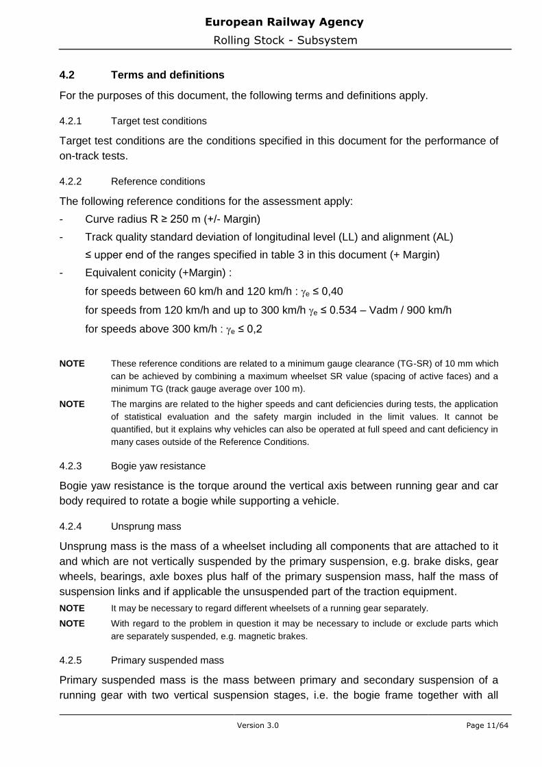
4.2 Terms and definitions
For the purposes of this document, the following terms and definitions apply.
4.2.1 Target test conditions
Target test conditions are the conditions specified in this document for the performance of
on-track tests.
4.2.2 Reference conditions
The following reference conditions for the assessment apply:
- Curve radius R ≥ 250 m (+/- Margin)
- Track quality standard deviation of longitudinal level (LL) and alignment (AL)
≤ upper end of the ranges specified in table 3 in this document (+ Margin)
- Equivalent conicity (+Margin) :
for speeds between 60 km/h and 120 km/h : e ≤ 0,40
for speeds from 120 km/h and up to 300 km/h e ≤ 0.534 – Vadm / 900 km/h
for speeds above 300 km/h : e ≤ 0,2
NOTE These reference conditions are related to a minimum gauge clearance (TG-SR) of 10 mm which
can be achieved by combining a maximum wheelset SR value (spacing of active faces) and a
minimum TG (track gauge average over 100 m).
NOTE The margins are related to the higher speeds and cant deficiencies during tests, the application
of statistical evaluation and the safety margin included in the limit values. It cannot be
quantified, but it explains why vehicles can also be operated at full speed and cant deficiency in
many cases outside of the Reference Conditions.
4.2.3 Bogie yaw resistance
Bogie yaw resistance is the torque around the vertical axis between running gear and car
body required to rotate a bogie while supporting a vehicle.
4.2.4 Unsprung mass
Unsprung mass is the mass of a wheelset including all components that are attached to it
and which are not vertically suspended by the primary suspension, e.g. brake disks, gear
wheels, bearings, axle boxes plus half of the primary suspension mass, half the mass of
suspension links and if applicable the unsuspended part of the traction equipment.
NOTE It may be necessary to regard different wheelsets of a running gear separately.
NOTE With regard to the problem in question it may be necessary to include or exclude parts which
are separately suspended, e.g. magnetic brakes.
4.2.5 Primary suspended mass
Primary suspended mass is the mass between primary and secondary suspension of a
running gear with two vertical suspension stages, i.e. the bogie frame together with all
European Railway Agency
Rolling Stock - Subsystem
Version 3.0 Page 12/64
components attached to it, e.g. braking equipment, antennas, pipes and cables plus half of
the primary and secondary suspension mass, half the mass of suspension links and
traction rods and if applicable the primary suspended part of the traction equipment.
NOTE With regard to the problem in question it may be necessary to include or exclude parts which are
separately suspended, e.g. magnetic brakes.
4.2.6 Secondary suspended mass
Secondary suspended mass is the mass supported by the secondary suspension of a
running gear, i.e. the relevant part of the carbody mass with all components attached to it,
e.g. upper bolster or adapter beam plus half of the secondary suspension mass, half the
mass of suspension links and traction rods and if applicable the secondary suspended part
of the traction equipment.
4.2.7 Bogie mass
Bogie mass is the mass of the bogie which rotates against the car body around the vertical
axis during the entrance into curves.
NOTE In most cases this mass is similar to the sum of the Unsprung Masses and the Primary
Suspended Mass of a running gear with two or more axles.
4.2.8 Yaw moment of inertia of whole running gear
The yaw moment of inertia of whole running gear is the moment of inertia of the mass.
4.2.9 Running behaviour
Running behaviour; the behaviour of a vehicle or running gear with regard to the
interaction between vehicle and track covering the specific terms running safety, track
loading and ride characteristics.
4.2.10 Equivalent conicity
Equivalent conicity (tane) is equal to the tangent of the cone angle tane of a wheelset with
coned wheels whose lateral movement has the same kinematic wavelength as the given
wheelset and is the relevant parameter of contact geometry on straight track and on large
radius curves (see also EN 15302:2008+A1:2010).
4.2.11 Operation envelope
The operation envelope is given by the combinations of speed and cant deficiency for
which the vehicle is intended to be operated.
4.2.12 Conventional technology vehicle
Conventional technology vehicles are vehicles which are operated under normal operating
conditions and correspond completely or in those construction parts which are relevant to
the Running Behaviour to the proven state of the art.

European Railway Agency
Rolling Stock - Subsystem
Version 3.0 Page 13/64
4.2.13 Reference vehicle
A reference vehicle is a vehicle that has the same fundamental design concept as the
vehicle to be assessed and that has been tested and approved in accordance with the
requirements of clauses 4.1 and 5 of EN 14363:2005 or in accordance with an equivalent
standard.
4.2.14 Engineering change
Engineering change is the change to the design of the vehicle that potentially varies the
performance of the vehicle, as evaluated by clauses 4.1 and 5 of EN 14363:2005.
4.2.15 Validation report
A validation report shows that the simulations based on the model of a vehicle provide a
good representation of its dynamic behaviour.
4.2.16 Simulation report
A simulation report is a report on the simulated dynamic performance of a vehicle.

European Railway Agency
Rolling Stock - Subsystem
Version 3.0 Page 14/64
4.3 Modified conditions
4.3.1 Loading conditions
For testing the vehicle in empty and/or loaded condition the following definitions apply:
Empty: Operational Mass in Working Order as specified in EN 15663:2009
Loaded: Design Mass under Normal Payload as specified in EN 15663:2009 Apart from this rule the loaded condition of passenger vehicles of long distance and high speed trains to be operated without obligatory seat reservation shall include 160 kg/m² (2 persons/m²) in standing areas instead of 0 kg/m². NOTE Special designed mass transit trains used in large and densely populated urban areas (like
some lines in Paris), where exceptional load as defined in EN 15663 occurs rather often, should include 700 kg/m² (10 persons/m²) in standing areas instead of 280 kg/m².
It is acceptable for all vehicles except locomotives that during the tests consumables are
reduced (e.g. due to fuel consumption) in a range that is normal for the operation of the
vehicle. For locomotives, only test results with a load above the operational mass in
working order according to EN 15663:2009 are acceptable.
4.3.2 Safety against derailment on twisted track
Compared to EN 14363:2005 clause 4.1 the requirements for testing safety against
derailment on twisted track shall be modified as following:
- Method 1 testing
o Assessment quantity in method 1 testing is only ∆z o The track layout presented in EN 14363:2005 must be understood as
example. It is only relevant to apply the test twist by the combination of test track and shims.
- Method 2 testing
o The combined test twist shall be applied in a way that the influence of shift of the centre of gravity due to twist is eliminated for the evaluated wheelset.
Based on test results of a Reference Vehicle a vehicle shall be accepted without testing,
either if
- the influence of the changes to the vehicle compared to the Reference Vehicle is
demonstrated and this shows that the acceptance criteria will not be exceeded,
or

European Railway Agency
Rolling Stock - Subsystem
Version 3.0 Page 15/64
- a calculation of guiding forces and vertical wheel forces for the Reference
Vehicle (for that tests were either performed under method 1 or method 2)
demonstrates credible results when compared with test results,
and
- the calculated result for the assessed vehicle remains 10 % below the limit value
(in a deflated suspension condition the 10 % margin does not apply),
and
- the calculated result does not increase by more than 1/3 of the margin between the test result and the limit value.
4.3.3 Requirements for assessment of fault modes
Compared to EN 14363:2005 clause 5.4.3.4 the way of handling of fault modes shall be
modified as following:
The criticality (the combination of probability and consequence) of fault modes shall be
analysed. The assumptions and results shall be reported. For each critical fault mode
identified it shall be clearly stated what the consequences in terms of the safety aspects
within the scope of this document would be and what, if anything, is required to be done in
terms of testing or other analysis.
If the criticality of a fault mode, considering any mitigation measures such as monitoring or
inspection, constitutes a risk higher than broadly acceptable, only safe behaviour shall be
demonstrated by tests, simulation or a combination of both. The extent of the test
procedure and/or the simulation cases shall be defined by reference to the analysis. If
simulation is used the conditions in Annex B must be fulfilled.
Possible fault modes to be considered include but are not limited to active suspension
systems, tilt systems, air suspension, yaw dampers…
Unless the analysis indicates a need for it (e.g. physical coupling), no superposition of
different fault modes needs to be considered.
For the fault modes it is sufficient to assess the criteria of running safety up to maximum
speed (Vadm) and maximum cant deficiency (Iadm).
If there is a low probability of occurrence of the considered fault mode based on the results
of the analysis, the safety margin included in the limit values of the assessment quantities
may be reduced. It is allowed to use specific limit values depending on the type of the fault
mode characteristics and their effects.
The test speed range and test cant deficiency range shall be adapted to appropriate
ranges.
If safe behaviour cannot be demonstrated for a relevant fault mode, control measures to reduce the criticality of the fault mode shall be defined to allow a safe operation.
NOTE Copied from EN 15827: Broadly acceptable risk is the “Level of risk that society considers trivial and is
consistent with that experienced in normal daily life and any effort to reduce the risk further would be
disproportional to the potential benefits achieved”.
European Railway Agency
Rolling Stock - Subsystem
Version 3.0 Page 16/64
4.3.4 Track quality
4.3.4.1 Basis of evaluation
The basis for the evaluation shall be the measured signals of track geometric deviation
obtained using normal track measuring methods with computerised recording and storage
according to EN 13848-1:2003+A1:2008 and EN 13848-2:2006 which specify the
wavelength ranges and required filter characteristics.
The data used for the evaluation of the track geometric quality shall be representative of
the maintenance status of the test track during the test.
4.3.4.2 Assessment quantities for track geometric quality
Track geometric deviations are measured for each rail. Evaluation variables of track
geometric deviation are:
a) alignment, lateral measuring direction
1) maximum absolute value Δy0max (mean to peak)
2) standard deviation Δy0σ
b) longitudinal level, vertical measuring direction
1) maximum absolute value Δz0max (mean to peak)
2) standard deviation Δz0σ
For test zone 1 the higher value of the two rails shall be used for the assessment of track
geometric quality. For test zones 2, 3 and 4 the values of the outer rail shall be used.
No requirements are given for track twist in the evaluation sections. However, if the track
twist in a section exceeds the safety limit value in EN 13848-5:2008+A1:2010 the section
may be excluded from the analysis.
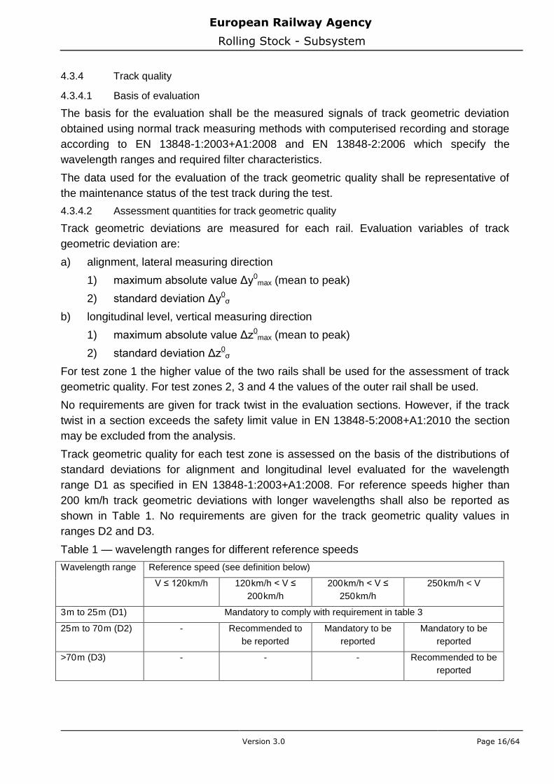
Track geometric quality for each test zone is assessed on the basis of the distributions of
standard deviations for alignment and longitudinal level evaluated for the wavelength
range D1 as specified in EN 13848-1:2003+A1:2008. For reference speeds higher than
200 km/h track geometric deviations with longer wavelengths shall also be reported as
shown in Table 1. No requirements are given for the track geometric quality values in
ranges D2 and D3.
Table 1 — wavelength ranges for different reference speeds
Wavelength range Reference speed (see definition below)
V ≤ 120 km/h 120 km/h < V ≤
200 km/h
200 km/h < V ≤
250 km/h
250 km/h < V
3 m to 25 m (D1) Mandatory to comply with requirement in table 3
25 m to 70 m (D2) - Recommended to
be reported
Mandatory to be
reported
Mandatory to be
reported
>70 m (D3) - - - Recommended to be
reported

European Railway Agency
Rolling Stock - Subsystem
Version 3.0 Page 17/64
4.3.4.3 Different Measuring Systems
If a measuring vehicle having a transfer function deviating from 1 or with a different
wavelength range is used for measurements, the track quality values shall be derived from
measured values subsequently corrected to be compatible with the above system.
There are two methods permitted for the correction:
a) The transfer function of the measuring system may be used to obtain absolute values
of measured track geometry. Here the measured signals are corrected using the
transfer function and are compared with the uncorrected values in table 2.
or
b) If a railway has no ability to correct the measured values directly it is also permitted to
use approximate scale factors k such that
- Standard deviation(other) = k. standard deviation(NS vehicle)
- The coefficients k to be applied in the wavelength D1 band from 3 m to 25 m can be
found in table 2 for certain measuring vehicles.
- The values in table 3 shall then be multiplied by the factors k of table 2 to give values
comparable with the other measuring system.
Table 2 — Correction factors for different track measuring vehicles
Measuring vehicle
Vertical alignment Lateral alignment
K Base K Base
High Speed Track Recording Coach
(HSTRC) 999550 – Mark 2f coach (BR)
1.14 inertial
(wavelength up to 35 m)
1.20 inertial
(wavelength up to 35 m)
GMTZ (DB) 1.24 2.6 m / 6 m 1.47 4 / 6 m
(RFI) 1.33 10 m 1.72 10 m
EM-120 (PKP) 0.73 10 m 0.71 10 m
MAUZIN cars 0.91 12.2 m 1.47 10 m
MATISA M562 0.91 12.2 m 1.47 10 m
4.3.4.4 Target test conditions
As the test results are related to the track conditions during the test, the target test
conditions shall be representative of the planned service operation. Therefore the
distributions in test zone 2, and separate or combined in zones 3 and 4 shall be such that
the 90 % values of the standard deviation of alignment and longitudinal level fall into the
ranges specified in table 3. In test zone 1 compliance with the above requirement is not
mandatory.

European Railway Agency
Rolling Stock - Subsystem
Version 3.0 Page 18/64
The reference speed for application of Tables 3 and 4 shall be determined in the following
way:
- Vadm for test zones 1 and 2;
- 80 km/h < V ≤ 120 km/h for test zones 3 and 4.
Table 3 — Target ranges for track geometric quality for international approval
Reference speed in
km/h
Target ranges for Standard deviation TL90 in mm
for wavelength range D1
Alignment y0 Longitudinal level z
0
Min Max Min Max
< V 80 km/h 1.95 2.70 2.75 3.75
80 km/h < V 120 km/h 1.05 1.45 1.80 2.50
120 km/h < V 160 km/h 0.75 1.00 1.40 1.85
160 km/h < V 200 km/h
200 km/h < V 230 km/h
0.70
0.65
0.90
0.80
1.15
1.05
1.60
1.45
230 km/h < V 300 km/h 0.50 0.65 0.85 1.15
Results from track sections with amplitudes of discrete defects higher than the stated QN3
values in table 4 may be excluded from the statistical evaluation to avoid a distortion of the
statistical analysis.
Table 4 — Limits for discrete track defects
Reference speed in km/h
Maximum absolute value (mean to peak) QN3 in mm
for wavelength range D1
Alignment y0max Longitudinal level z
0 max
< V 80 km/h 18.2 20.8
80 km/h < V 120 km/h 13.0 15.6
120 km/h < V 160 km/h 10.4 13.0
160 km/h < V 200 km/h 9.1 11.7
200 km/h < V 300 km/h 7.8 10.4
NOTE Tables 3 and 4 contain requirements for international approval. For local, national or
multinational operation the values may be varied.
NOTE The values in table 4 are taken from EN 14363:2005, therefore only 200 km/h is used as interval
boundary, whereas in table 3, 230 km/h is used in addition.
NOTE For speed above 300 km/h, the target test conditions shall correspond to better track quality
than the track quality specified for the speed 300 km/h.
The values met on the test track shall be reported as required in clause 4.3.4.5; corresponding
operating limitations shall also be reported as required in clause 4.1.
For the evaluation of track geometric deviations in the test route, the track sections
selected for the testing of running characteristics shall be used.
Two analysis methods may be used:
- 1st method (recommended):

European Railway Agency
Rolling Stock - Subsystem
Version 3.0 Page 19/64
The track sections used for the analysis are the same as those selected for the
statistical evaluation of the vehicle behaviour.
- 2nd method:
The track sections used for the analysis are derived from standard data from track-
measuring vehicles (e.g. standard deviations in 200 m sections). In this case, it is not
possible for track-related and vehicle-related sections to strictly coincide. The track
quality data shall be assigned in the most appropriate way to the track sections used
for evaluation of the test results. The process used shall be stated in the test report.
NOTE For zones 3 and 4 it is strongly recommended to use the first method. In order to improve upon
this, the use of standard deviation sliding values is recommended, with a rather low sliding
interval such as 10 m for example.
4.3.4.5 Reporting
For each test zone a graphical representation of standard deviation values of vertical
alignment and lateral alignment in the wavelength range D1, section by section, together
with the 90 % values, shall be given in the report. A table of these values may also be
included.
It shall be stated in the report, if any sections were excluded from the analysis due to
amplitudes higher than the stated QN3 values. A list of such excluded sections shall be
given in the report including information about radius, speed, cant deficiency and the four
track geometric quality values.
4.3.5 Stability testing
Stability testing shall be performed on tangent track with high conicities. If these tests are
performed separately, the application of the simplified measuring method is sufficient as
the method is consistent with the normal measuring method.
NOTE This allows to achieve the required high conicity condition also by modification of the wheel
profile on a running gear without instrumented wheelsets and to keep normal profiles on the
instrumented wheelset.
NOTE In this case the instrumentation of running gear (or in the case of a vehicle with single axle
running gear: with instrumentation on the car body) is sufficient.
NOTE If a vehicle is equipped with an instability monitoring system based on lateral accelerations,
results collected by this system may be used to demonstrate running stability.
4.3.6 Contact Conditions
Wheel profiles representative for the service of the vehicle shall be used during testing. In
that case the range of contact conditions varies sufficiently for the statistical evaluation due
to variations of gauge and rail shape on test lines. The following conditions related to the
contact conditions during on-track test apply to replace testing in networks with two
different rail inclinations. As an alternative to performing on-track tests on two different rail
inclinations, as set out in paragraph 5.4.4.4 in EN 14363:2005 it is permitted to perform
tests on only one rail inclination if demonstrated that the tests cover the range of contact
conditions defined below:

European Railway Agency
Rolling Stock - Subsystem
Version 3.0 Page 20/64
4.3.6.1 Requirements for tangent track (Test zone 1)
1. Tests shall be carried out
a. considering stability testing, on at least 300 m track length where equivalent conicity (with the representative tested wheel profile) is greater than or equal to the values given below, depending on the speed
i. For speeds between 60 km/h and 120 km/h : tan(e) ≥ 0,40
ii. For speeds from 120 and up to 300 km/h : tan(e) ≥ 0,534-V/900 km/h
iii. For speeds higher than 300 km/h : tan(e) ≥ 0,2
NOTE A possible representation of observed conditions consists in a bar chart with representative values per track
section.
NOTE These target test conditions are related to a minimum gauge clearance (TG-SR) of 10 mm which can be
achieved by combining a maximum wheelset SR value (spacing of active faces) and a minimum TG (track
gauge average over 100 m).
NOTE In some cases national systems, either parts or all, cannot comply with these Reference Conditions for
equivalent conicity in the short or medium term. These cases are outside the scope of this document.
Nevertheless the process defined in EN 14363:2005 amended by this document for the proof of running
stability can also be used for higher equivalent conicities. In these cases safety maybe demonstrated by
application of existing national requirements for high equivalent conicities during stability testing.
b. On the whole test zone 1 the majority of the conditions shall be representative for normal service. A narrow range of contact geometry conditions shall be avoided.
Requirements for measuring of rail profiles and evaluation of equivalent conicity are
specified in Annex D.1
4.3.6.2 Requirements for test zones 1 and 2
Considering testing for low frequency body motions, track sections with the maximum
value <0.05 and a track gauge clearance (TG-SR) ≥ 8 mm shall be included in the
assessment.
4.3.6.3 Requirements for very small curve radii (Test zone 4)
A narrow range of contact geometry conditions shall be avoided.
4.3.7 Target cant deficiency for the evaluation of quasistatic assessment quantities
For the estimated quasi-static values (k = 0) the two-dimensional method shall be used
and values shall be assessed at the regression line for 1.00 x Iadm.
4.3.8 Test speed for vehicles with Vadm>300 km/h
The test speed for vehicles with Vadm > 300 km/h is Vadm + 30 km/h.
4.3.9 Multiple regression against target test conditions
This method (see Annex A) in its full extension can replace the two-dimensional evaluation
as in many cases the assessment quantities depend more on other input quantities than
the cant deficiency. On the other hand, the 2-dimensional evaluation is a special case of
the full multiple regression with only one input parameter (cant deficiency).
NOTE If dependency parameters are chosen carefully, a sufficient confidence in calculated estimated values is
achievable.

European Railway Agency
Rolling Stock - Subsystem
Version 3.0 Page 21/64
4.3.10 Alternative evaluation for Y/Q
In the event that the limit value Y/Qa,max = 0,8 is exceeded or if < 1.1, it is permissible to
recalculate the test results and use the result for comparison with the limit value.
The recalculation shall be carried out according to the following process.
• create an alternative test zone made up of all track sections with 300 m ≤ R ≤ 500 m
• for the statistical processing per section, use h1 = 2.5 % instead of h1 = 0.15 % and
h2 = 97.5 % instead of h2 = 99.85 %
• for the statistical processing per zone replace k = 3 by k = 2.2, when using one-
dimensional method
• confidence level PA = 99.0 % by PA = 95.0 %, when using two-dimensional method.
4.3.11 Evaluation of quasistatic guiding force Yqst
The evaluation of the estimated value for the guiding force is performed in two steps of
which the first step may not be necessary:
1) If during the test some individual (Y/Q)i.50% values exceeded 0.40, the estimated
value may be normalised:
In track sections where (Y/Q)i,50% exceeds the value of 0.40 replace the
frequency values Ya,50% on the outer rail of the track sections by:
Ya,f,50% = Ya,50% – 50 kN[(Y/Q)i,50% – 0.4]
Afterwards calculate the estimated value normalised by friction Yf,qst
NOTE The normalisation takes into account roughly 50% of the physical influence of values of Y/Q i above 0.4 on
the increase of the guiding force.
NOTE The normalisation can only be performed for Y/Qi values above 0.4 as Y/Qi represents friction only in case
of saturation of the creep force law.
2) For test zone 4 the test results Yqst (and Yf,qst) with a given mean curve radius
Rm shall be normalised to the Reference Condition (Rmr = 350 m) by the
following formulae:
YR,qst = Yqst – (10500 m / Rm – 30) kN
Yn,qst = Yf,qst – (10500 m / Rm – 30) kN (only if (Y/Q)i,50% exceeds 0.4)
Rm indicating the mean radius of all track sections in the test zone.
For comparison with the limit value, the most normalised value shall be used.
NOTE The specified limit is not a running safety relevant limit but has to be considered in relation to the
load/mechanical strength and the wear of the international, multinational or national design of the
superstructure.
European Railway Agency
Rolling Stock - Subsystem
Version 3.0 Page 22/64
4.3.12 Evaluation of additional track loading parameters
In addition the following parameters shall be documented (no limit values are specified): Combined rail loading quantities:
- Bqst = Yn(R),qst + 0.83 Qqst - Bmax = |Y| + 0.91 Q - Maximum guiding force Ymax
NOTE These parameters can help to determine acceptable operating and vehicle conditions (cant deficiency,
speed, friction conditioning, payload) depending on track layout, track design, track quality and track maintenance strategy.
4.4 Methods to assess the vehicle against missing target test conditions
4.4.1 Operating envelope
When planning on-track tests, the operational limiting parameters Vadm and Iadm for the
vehicle have to be selected by the applicant. The chosen values determine the future use
of the vehicle. It may be necessary to test a vehicle for more than one combination of Vadm
and Iadm. The assessed combinations shall be reported.
4.4.2 Track section length Lts
Deviating from EN 14363:2005, tables 8 and 9 in test zones 1 and 2 a track section length
Lts of only 100 m may be used up to a speed of 160 km/h.
A tolerance for the length of the individual test section Lts of ±20% may be applied to all
test zones. The minus tolerance may only be used, if it permits additional track length to
be included in the analysis.
4.4.3 Minimal number of track sections nts,min in test zone 3
As for the other test zones it is also for test zone 3 sufficient to evaluate the estimated
value from 25 track sections (see EN 14363:2005, table 9).
4.4.4 Minimal total length of track sections Lts,min in test zone 2
Deviating from EN 14363:2005 it is sufficient to include 5 km total track length into the
statistical evaluation for test zone 2.
4.4.5 Methodology, when the minimum number of sections nts,min is not fulfilled in a test zone
For the application of this process, it is required that the estimated maximum values (k ≠ 0)
are evaluated by the one-dimensional method.
When this minimum number of sections nts,min cannot be reached as required by EN
14363:2005 and complemented by this document, it is possible to use the results from the
reduced data set as a basis for evaluation by increasing the estimated values. For the

European Railway Agency
Rolling Stock - Subsystem
Version 3.0 Page 23/64
estimated maximum values (k ≠ 0), according to the actual number of sections nts, choose
C(nts) for each assessment quantity using the table below:
Table 5 - Correction factors C(N) for N = 25 to 15 sections
Assessment
quantity ≥ 25 24 23 22 21 20 19 18 17 16 15
Safety related
quantity 1 1.007 1.015 1.024 1.034 1.044 1.056 1.069 1.083 1.099 1.118
Other quantities 1 1.004 1.007 1.011 1.016 1.020 1.026 1.031 1.038 1.045 1.053
Extrapolation outside the given range of N in each table is not allowed. The new estimated
maximum value is: Yc,max = C(N) x Ymax
As the two dimensional evaluation method uses already the student t factors depending
on the sample size no further correction is necessary. The minimum number of sections is
15.
For the quasi-static values (k=0) calculated by the two-dimensional method using the
cant deficiency as variable it is possible to use the results from the reduced data set as a
basis for evaluation, by increasing the estimated values Yc(X0).
When X = X0, the mean value of Y equals the value given by the linear regression, i.e.
Yc(X0) = a + bX0.
Also when X = X0, the bounds within which Y will fall with a certain probability can be found
by using a Student bilateral distribution t’, in which Yp is the predicted value of Y:
)('
)('
0
0
XS
YXYt
Y
pc
with N-2 degrees of freedom, where N stands for the number of (X,Y) pairs for which:
22
2
0)(
)(1)('
XXN
XXoN
NSXS eY
Se representing the scatter of the Y values about the regression line for all values of X,
SY Y
Ne
c
( )2
2
Due to the bilateral confidence interval selected (95 % for the track fatigue and running
behaviour quantities), the value of the correction factor C’(N) = t’N – t’25 or t’N – t’50 to be
applied is given in the tables below (for other values of N, refer to literature):

European Railway Agency
Rolling Stock - Subsystem
Version 3.0 Page 24/64
Table 6 - Correction factors C’(N) for N = 25 to 15 sections
Number of sections (N) 15 16 17 18 19 20 21 22 23 24
Student t’ factor (95 %) 2.160 2.145 2.131 2.120 2.110 2.101 2.093 2.086 2.080 2.074
Correction factor C’(N) 0.091 0.076 0.062 0.051 0.041 0.032 0.024 0.017 0.011 0.005
The new estimated quasi-static value is the corrected value corresponding to I = 1.00 Iadm,
in other words: )(')(')()(ˆ 000 XSNCXYYXY Ycp .
4.4.6 Improve relevance of estimated value in 2-dimensional evaluation
The narrow band of cant deficiency as specified in EN 14363:2005 is appropriate when
using the one-dimensional method but may lead to low significance of the regression line
when using the two-dimensional method. Therefore it is recommended to include also
tests with cant deficiencies below 0,70 Iadm when using the two-dimensional method. In
that case the multiple use of the same track section within the same zone (2, 3 or 4) is
permitted as well as using additional track sections for test zones 3 or 4.
The following conditions apply:
- nts,min and Lts,min as specified in EN 14363:2005 shall be reached and the given cant deficiency distribution shall be achieved taking into account the number of unique track sections (nts) within the cant deficiency range defined for the test zone in
EN 14363:2005.
- For multiple use of the same section the cant deficiency shall differ by at least
0.05 Iadm.
- The mean radius Rm (for zones 3 and 4) specified in EN 14363:2005 shall be evaluated taking into account all the occurrences of every track section.
- All data added by multiple use or additional sections shall be such that I > 40 mm and the total number of additional sections shall not be larger than nts.
- The number of sections below 0.7 x Iadm shall be less than 50 % of the total number of sections.
- The speed requirements stated in EN 14363:2005 for test zone 2 are applicable for all track sections used.
NOTE The aim to improve confidence is missed, if the distribution of the data along the regression line is uneven
or have a concentration at the lower end of the regression line.
4.4.7 Use of simulation to complement investigations for a proper assessment
The initial assessment of the dynamic performance of a vehicle type shall generally be
based on on-track tests. In certain circumstances these tests may be supplemented by
simulation (see Annex B) or other means, e.g. when the combination of the target test
conditions cannot be achieved during the test.

European Railway Agency
Rolling Stock - Subsystem
Version 3.0 Page 25/64
4.4.8 Multiple regressions against target test conditions
It is sometimes the case that, on a test zone:
1. the number of test track sections individually complying with the specifications of the test procedure is sufficient, but the test zone as a whole does not meet the target values for curve radius (mean value), cant deficiency (80th percentile) or track geometry (90th percentiles),
2. and/or the requested number of test track sections can only be reached after including invalid sections (outside the requested ranges of curve radius, speed or cant deficiency).
Then the estimated values of assessment quantities on this test zone do not reflect
vehicle’s behaviour in the operating conditions in which it should be assessed.
It is possible to use only the valid track sections, meeting the requirements both
individually and collectively, and then:
- applying correction factors taking into account the insufficient number of sections,
- or complementing the sample using numerical simulation on additional sections.
The use of multi linear regressions allows in both cases 1 and 2 above to estimate the
result under the required conditions.
The principle of this method is to investigate the correlations between the assessment
quantities and their influence parameters, in order to extrapolate the estimated values of
these assessment quantities to the target values (not achieved during the test) of these
influence parameters.
A first method, described in Annex A.3, consists in correcting the values obtained using a
one- or two-dimensional method. A second method, described in section A.4 and assumed
to be more accurate, uses a multi-linear analysis to determine the estimated values.
4.4.9 Extension of acceptance / Instrumentation of trainsets
An extension of acceptance for vehicles that are of the same basic design, or that have
gained acceptance and subsequently undergone Engineering Change, is possible. If a
dispensation from assessment is not possible, the assessment shall be carried out either
by means of a partial on-track test or by simulation of an on-track test or a combination of
both. The procedure (test extent and measuring method) to be applied for the partial on-
track test (including dispensation from test) is defined in Annex C and for simulation in
Annex B.

European Railway Agency
Rolling Stock - Subsystem
Version 3.0 Page 26/64
Annex A Determination of estimated values using multi linear evaluation
A.1 Technical and statistical theory
It is sometimes the case that, on a test zone:
1) the number of test track sections individually complying with the specifications of
the test procedure is sufficient, but the test zone as a whole does not meet the
requirements for the distributions of cant deficiency, curve radius or track quality,
2) and/or the minimum number of test track sections can only be reached after
including invalid sections (outside the requested ranges of speed, cant deficiency or
curve radius).
Then the estimated values of assessment quantities on this test zone do not reflect
vehicle‘s behaviour in the operating conditions in which it should be assessed.
It is possible to use only the valid track sections, meeting the requirements both
individually and collectively, and then:
apply correction factors accounting for the insufficient number of sections (see 4.4.5),
or complement the sample using numerical simulation on additional sections (see
Annex B).
Alternative methods, described hereafter, allow in both cases 1 and 2 above to estimate
the results under the required conditions. Their principle is to use multi linear regressions
to investigate correlations between the assessment quantities and their influence
parameters, in order to extrapolate the estimated values of these assessment quantities to
the target values (not achieved during the test) of these influence parameters.
On each test zone and for each assessment quantity, the influence parameters to be used
in the multi linear regression are quoted in Annex A.2, together with:
the range allowing the use of a track section in the analysis (usually wider than in the
one-dimensional method),
the target value at which the assessment quantity shall be evaluated.
A first method, described in Annex A.3, allows correcting the values obtained using a one-
or two-dimensional method. A second method, described in section A.4 and assumed to
be more accurate, uses a full multi-dimensional analysis to determine the estimated
values.
A.2 Test conditions – allowed ranges for the evaluation
The analysis should be restricted to the input parameters for which there exists a target
value or range. These parameters are the following:

European Railway Agency
Rolling Stock - Subsystem
Version 3.0 Page 27/64
- speed V on test zones 1
- radius R on test zones 3
- track quality AL and LL on all test zones
The table A.1 summarises the parameters to be used for the multi linear regression,
according to the test zone and the assessment quantity considered:
Table A.1 — Selection of parameters
In order to improve the regressions:
each test zone may be extended using additional track sections (see conditions below),
all the input parameters used should be distributed as evenly as possible over the whole allowed ranges,
when curve radii of track sections in test zones 3 and 4 do not properly cover their full respective ranges (400 - 600 m and 250 - 400 m), these two test zones shall be merged for the performance of multi linear regressions.
Every track section used for the multi linear analysis shall fulfill the following requirements: Speed: 0.50xVadm ≤ V ≤ 1.10xVadm + 5 km/h (test zones 1 and 2) Cant deficiency: 40 mm ≤ I ≤ 1.15xIadm (test zones 2, 3 and 4) Curve radius: 400 m ≤ R ≤ 600 m (test zone 3)
250 m ≤ R < 400 m (test zone 4) Track quality: no specific requirement

European Railway Agency
Rolling Stock - Subsystem
Version 3.0 Page 28/64
In addition, 5 or more track sections used shall meet the following requirements:
On test zone 1: V ≥ 1,05xVadm On test zone 2: V ≥ Vadm - 5 km/h and I ≥ 1,05xIadm On test zone 3: I ≥ 1,05xIadm On test zone 4: I ≥ 1,05xIadm and R ≤ 300 m On test zones 3 and 4 when merged : I ≥ 1,05xIadm and R ≥ 500 m on ≥ 3 sections and I ≥ 1,05xIadm and R ≤ 300 m on ≥ 3 sections The target values for these parameters are the following: Speed: V = MIN(1.10xVadm; Vadm+30 km/h) (on test zone 1)
V = Vadm (on test zone 2) Cant deficiency: I = 1.10xIadm (for maximum values)
I = Iadm (for quasi-static values) Curve radius: R = 500 m (on test zone 3)
R = 350 m (on test zone 4)
Track quality: AL or LL = TL90min (for the application of A.3)
AL or LL = 0.90xTL90min (for the application of A.4)
A.3 Specified process for the correction of estimated values
When the assessment was carried out according to the one-dimensional method or the
two-dimensional method using cant deficiency as input variable, a correction may be
necessary. The field of application is described in A.1 (cases 1 and 2).
The process is the following, the example of Y1 on test zone 4 being used for illustration.
a) If this is relevant, additional track sections are added to the test zone(s) - see A.2.
b) A multi linear regression of every assessment quantity (99.85 % or 50 % values on
every track section shall be used) is performed, using the parameters identified as
relevant to explain this assessment quantity on this test zone - see Table A.1.
c) A regression formula is derived, of the type: (ΣY1)99,85% = a0 + a1 / R + a2 · I + a3 · σAL
d) The original (one- or two-dimensional) estimated value is corrected, using the
coefficients of this regression formula together with the differences between the target
values of the influence parameters (stated at the end of A.2) and the values observed
on the sample of track sections used in the original (one- or two-dimensional) analysis.
European Railway Agency
Rolling Stock - Subsystem
Version 3.0 Page 29/64
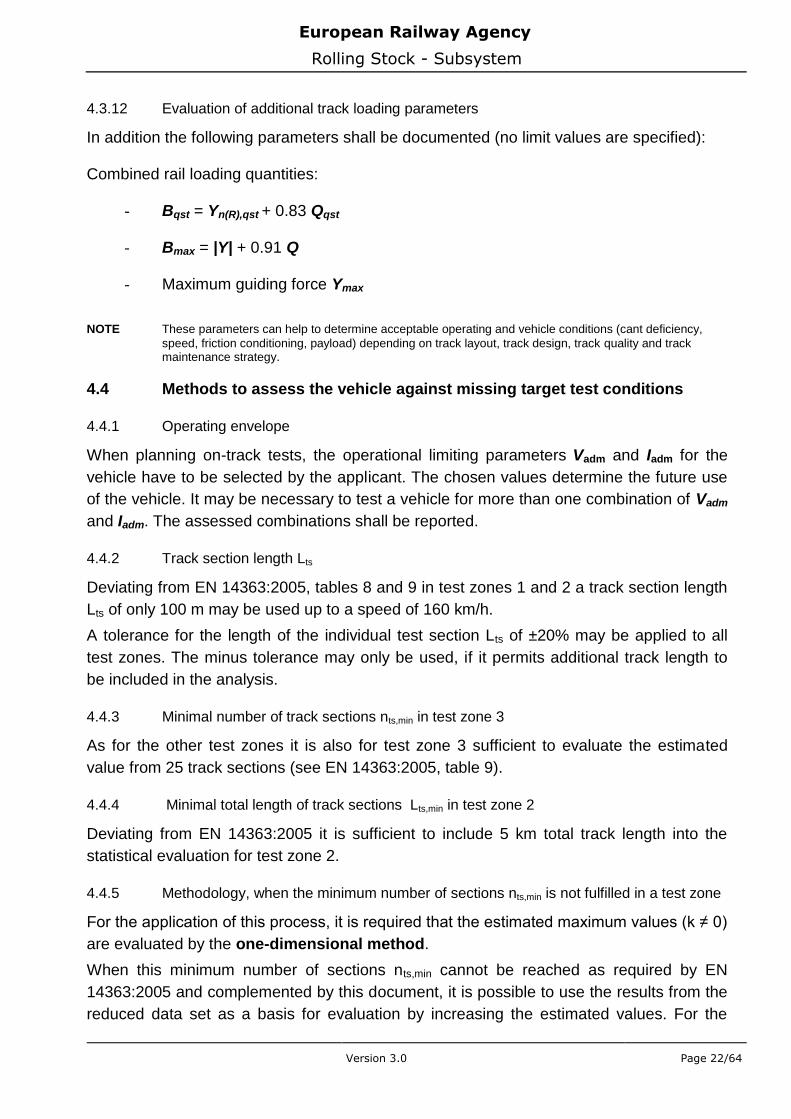
For this purpose, the observed values to be taken into account are:
the mean value of speed V (test zone 1 or 2)
the 90th percentile of cant deficiency I (test zone 2, 3 or 4)
the mean value of radius R (test zone 3 or 4)
the 90th percentile of track quality AL or LL (any test zone) In our example, if on test zone 4:
the mean radius of the test sections used was 375 m (target: 350 m),
the 90th percentile of cant deficiencies was 145 mm (target: 165 mm),
the 90th percentile of alignment was 0.70 mm (target: 1.05 mm),
then the maximum estimated value of Y found on test zone 4 shall be increased by: a1.(1/350 - 1/375) + a2.(165 - 145) + a3.(1,05 -0,70) before being compared to the limit value (10 + P0/3). When the estimated value was obtained using the two-dimensional method, no correction according to cant deficiency shall be introduced (cant deficiency being already normalised).
(1) the regression work may be performed for test zones 3 and 4 together (it usually
increases the relevance of the equation), but other steps shall be carried out separately on
each zone, as the results to be corrected and the target conditions are different.
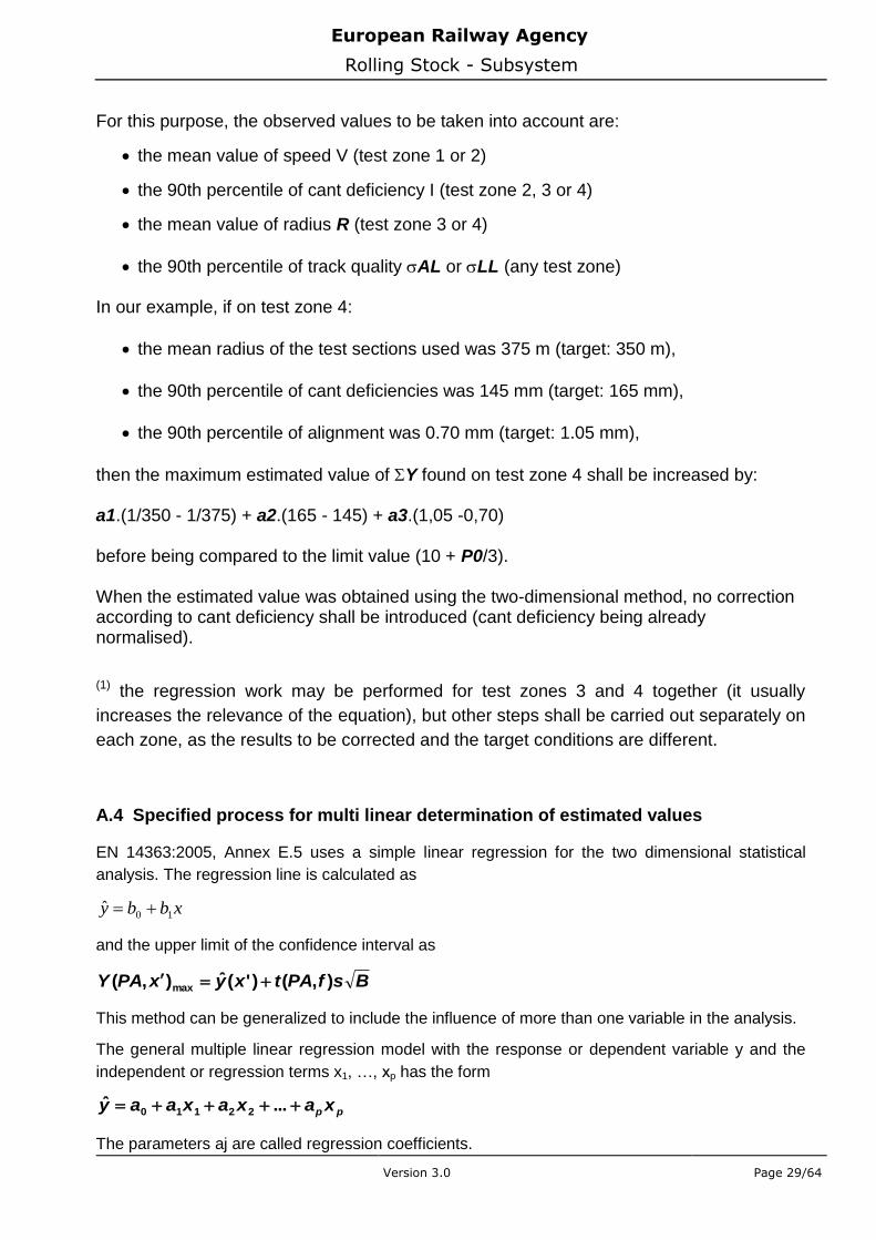
A.4 Specified process for multi linear determination of estimated values
EN 14363:2005, Annex E.5 uses a simple linear regression for the two dimensional statistical
analysis. The regression line is calculated as
xbby 10ˆ
and the upper limit of the confidence interval as
BsfPAtxyxPAY ),()'(ˆ),( max
This method can be generalized to include the influence of more than one variable in the analysis.
The general multiple linear regression model with the response or dependent variable y and the
independent or regression terms x1, …, xp has the form
pp xaxaxaay ...ˆ22110
The parameters aj are called regression coefficients.

European Railway Agency
Rolling Stock - Subsystem
Version 3.0 Page 30/64
For the calculation of the regression coefficients a matrix notation can be used were we find
Xay
with
ny
y
y
y2
1
measured values of the dependent variable
,
nknn
k
k
xxx
xxx
xxx
X
21
22221
11211
1
1
1
Matrix of the measured values of the input variables
,
ka
a
a
a1
0
regression coefficients
The least square estimate a of the regression coefficients a can be calculated by solving the least
square equation
yXXXa 1)(ˆ
Most of the standard technical software tools have algorithms included for performing this
calculation like rgp in Microsoft Excel and regstats in MATLAB.
The special case of only one regression term (p=1) can also be derived from this equation. This
leads to the formulae in EN 14363:2005, Annex E.5.
The upper limit of the confidence interval at x=x0 can be calculated as
YXbYYRSS
pn
RSSs
xXXxsfPAtxyxPAY
ˆ
)1(
)(1),()(ˆ),(
2
0
1
00max0
with
02021010ˆ...ˆˆˆˆ
ppxaxaxaay
as estimate of the regression value at x0 and
t(PA,f) as threshold value of the bilateral t-distribution.
The estimated value is calculated at the regressor values xio equal to the target conditions as
stated in Annex A.2.
European Railway Agency
Rolling Stock - Subsystem
Version 3.0 Page 31/64
NOTE The two-dimensional method is an example of multi linear regression, where only one input
parameter (cant deficiency I) is used (p = 1). The principles and equations given in this section
remain valid and lead to the formulae in EN 14363:2005 annex E.5.
A.5 Documentation
Data used for multi linear analyses shall be documented. For each test zone (or merged zones 3 and 4) a table shall provide, as a minimum, for each track section used in the multi linear regressions:
speed V (on test zones 1 and 2),
cant deficiency I (on test zones 2 - 3 - 4),
radius R and/or curvature 1/R (on test zones 3 and 4),
track quality AL and LL (on all test zones),
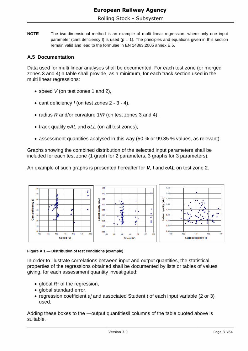
assessment quantities analysed in this way (50 % or 99.85 % values, as relevant). Graphs showing the combined distribution of the selected input parameters shall be included for each test zone (1 graph for 2 parameters, 3 graphs for 3 parameters).
An example of such graphs is presented hereafter for V, I and AL on test zone 2.
Figure A.1 — Distribution of test conditions (example)
In order to illustrate correlations between input and output quantities, the statistical properties of the regressions obtained shall be documented by lists or tables of values giving, for each assessment quantity investigated:
global R² of the regression,
global standard error,
regression coefficient aj and associated Student t of each input variable (2 or 3) used.
Adding these boxes to the ―output quantities‖ columns of the table quoted above is suitable.
European Railway Agency
Rolling Stock - Subsystem
Version 3.0 Page 32/64
Annex B Simulation
B.1 Introduction
The dynamic performance of the vehicle must normally be verified by tests (static tests
and on-track tests), but the use of simulation in place of on-track test is permitted under
controlled conditions. The objective when using simulation is to achieve the same level of
confidence in the results as would be achieved by on-track tests. The simulation process
described in this annex sets out one means by which this can be achieved. Other
simulation procedures that achieve the same level of confidence are also permitted.
NOTE The range of conditions of the validation determines the scope for which the model is then approved for
simulations. Therefore it is recommended that the simulation validation covers the widest practical range of
test conditions.
B.2 Scope
B.2.1 General
Four cases of application where numerical simulations can be used in place of testing are
detailed in this Annex. These are:
- extension of the range of test conditions where the full test programme has not been completed,
- verification of vehicle dynamic behaviour following modification,
- verification of new vehicles dynamic behaviour by comparison with an already approved Reference Vehicle,
- investigation of dynamic behaviour in case of fault modes.
The scope of these cases of application and the conditions for use of numerical simulation
is described in the following sub-clauses. Other cases of application may exist.
NOTE It is possible to perform simulations in order to determine the vehicle behaviour on track conditions differing
from the tested conditions, e.g. to cover the conditions in different countries.
A vehicle model has to be developed and validated by comparison with the available test
results in accordance with B.3.
B.2.2 Extension of the range of test conditions
Where on-track tests according to EN 14363:2005 including any modification to the test
conditions as set out in this Technical document have been carried out, but the full range
of test conditions has not been satisfied, then it is permissible to use numerical simulations
to cover the deficiencies as part of the vehicle running dynamic behaviour verification. This
situation could arise where:
- sufficient track length is not available to meet the requirements for some zones,
- the full range of speed and cant deficiency has not been tested,

European Railway Agency
Rolling Stock - Subsystem
Version 3.0 Page 33/64
- the full range of wheel-rail contact conditions has not been covered,
- measuring channels failed, or provided unreliable results.
It is permitted to use numerical simulations for a single or multiple test zones where the
test results are not complete.
B.2.3 Verification of vehicle dynamic behaviour following modification
Vehicle modifications may be carried out for a number of different reasons, for example:
- change of the use of the vehicle,
- upgrade of the vehicle,
- modifications to improve the running behaviour:
a. during or following the test programme,
b. when some tests were done in a preliminary vehicle configuration and the final configuration is defined afterwards.
A model of the original vehicle is developed and validated against the test results for that
vehicle in accordance with clause B.3. The model of the vehicle is then modified to
represent the physical changes to the vehicle as a result of the modification. Only the
changes that influence the dynamic behaviour are required to be included in the modified
model. The revised model is used to simulate the dynamic behaviour and the results are
compared with the limit values for assessment.
Simulations for all test zones have to be carried out to demonstrate that the vehicle
performance of the new vehicle is consistent when compared to the previously tested
vehicle. The influence that the changed parameter(s) has (have) on the dynamic
performance has to be examined for all zones. The results of this examination must be
reported and the influence on the performance indicated.
If a vehicle has been tested according to EN 14363:2005 including any modification to the
test conditions as set out in this Technical document and found to exceed some of the limit
values, then it is permitted to use numerical simulations to demonstrate that modifications
to the vehicle will improve the behaviour sufficiently to meet the limits. The values that
previously exceeded the limits have to be under the limit values for track loading and at
least 10 % below the limits for running safety. At the same time all other values must
remain below the limit and not increase by more than 1/3 of the previous margin to the limit
value. In this situation the vehicle can be regarded as acceptable for the previously
deficient limit values.
The data from the simulation is to be used to assess the modified vehicle.
B.2.4 Verification of new vehicles dynamic behaviour by comparison with an already approved Reference Vehicle
Where vehicles are being introduced with a range of different types within the fleet (e.g.
multiple units, etc.) then one vehicle type is defined as the Reference Vehicle. The running
European Railway Agency
Rolling Stock - Subsystem
Version 3.0 Page 34/64
dynamic behaviour of vehicles that are similar to the Reference Vehicle can then be
verified by numerical simulations, rather than by on track tests.
Model(s) of the new vehicle(s) that are to be assessed are to be developed from the
Reference Vehicle.
The existing and changed parameters are to be included in the simulation to demonstrate
the influence of the changes on the performance.
Simulations for all test zones are carried out to demonstrate that the vehicle performance
of the new vehicle is consistent when compared to the Reference Vehicle. The influence
that the changed parameter(s) has (have) on the dynamic performance is to be examined
for all zones. The results of this examination are to be reported and the influence on the
performance indicated.
If as result of the changes the dynamic response of the new vehicle does not increase any
assessment value compared to the Reference Vehicle and the changes do not
fundamentally affect the frequency or amplitudes of the dynamic response, then the
influence of the change on the dynamic performance is considered insignificant. The
model can be used for vehicle approval.
If the change to the dynamic performance results in
- an increase in any assessment value compared to the Reference Vehicle,
- and/or a fundamental change in the frequency and/or amplitudes of the dynamic response,
then a full review must be carried out.
This review must include analysis that investigates the changes to the dynamic
response(s) of the new vehicle compared to the Reference Vehicle and an associated
explanation of the effects identified. This comparison has to be carried out for at least 3
sections of each test zone, if it demonstrates that
- the assessment values for running safety from simulations do not increase by more than 1/3 of the previous margin to the limit values,
- and at the same time the values for track loading from simulations do not increase by more than 2/3 of the previous margin to the limit values,
then the simulation can be used for vehicle approval.
NOTE Changes to individual components such as springs or dampers are likely to be acceptable provided the
characteristics of the changed components are known and the changes are not extreme. Limited changes to
masses, inertias or centres of gravity are also likely to be acceptable. A change to the concept of the suspension or introduction of components which were not present in the validated model for the tested
vehicle is less likely to be acceptable.
B 2.5 Investigation of dynamic behaviour in case of fault modes
The use of simulation to investigate fault modes in support of verifying the running
dynamic behaviour characteristics of a vehicle is permitted. The process of selecting and

European Railway Agency
Rolling Stock - Subsystem
Version 3.0 Page 35/64
assessing fault modes is independent from the assessment method (test method or
simulations).
The model must only be used within its range of validity.
B.3 Validation
B.3.1 General principles
Models used in numerical simulations are required to be validated by comparison with test
results from the vehicle that is being modelled.
Information that is required to carry out the validation shall include:
- Design data for the modelled vehicle that is sufficiently detailed to enable the features that influence the vehicle dynamics to be incorporated into the model.
- Test results for the modelled vehicle in a form that can be used for model validation including time history data in a digital form. It is necessary that these tests and data include a representative range of track conditions, curves, cant deficiency, speed and wheel/rail contact conditions.
- Track data from the original test route to enable validation to be undertaken.
B.3.2 Vehicle model
The model must include the main components such as wheelsets, bogies/running gear,
vehicle body and all of the relevant connections between them (e.g. geometry, linear/non
linear stiffness, damping, clearances, etc). Data describing the vehicle body has to be
included to the level of detail required to represent dynamic effects that are prominent in
the dynamic performance (e.g. masses, inertias, position of centre of gravity, significant
eigenmodes/flexible bodies).
The precision and level of detail that is appropriate in a model will depend on the particular
assessment values that are to be evaluated.
B.3.3 Validation of the vehicle model
B.3.3.1 Introduction
Generally, numerical simulations require, in order to generate valid results, that:
- the vehicle model is a good representation of the actual vehicle,
- the software used is appropriate for the application,
- the correct conditions have been covered.
If numerical simulations are to be used for a vehicle in different conditions (for example
tare, laden, inflated, deflated, …), separate models will need to be validated for each
condition.

European Railway Agency
Rolling Stock - Subsystem
Version 3.0 Page 36/64
B.3.3.2 Validation process
The validation process is based on comparisons between physical test results of the
vehicle and numerical simulations of the same tests. The primary purpose of validating a
numerical vehicle model is to use that model to simulate the vehicle behaviour in-lieu of
actual on-track tests. Vehicle approval requires the assessment of the vehicle's static,
quasi-static and dynamic behaviour. Therefore the model has to include validation against
the static, quasi-static and the dynamic tests.
NOTE The range of conditions of the dynamic validation determines the scope for which the model is
then approved for simulations. Therefore it is recommended that the validation tests and
simulation comparisons cover the widest practical range of conditions.
The validation process shall also be made across the appropriate dynamic frequency
range. All comparisons between simulation and actual on track test results have to be
made using the same vehicle model and software. A model that has been validated must
not be changed for subsequent simulations, except for the conditions given in B.2.3 and
B.2.4.
It is required that the results of all appropriate work carried out to validate the vehicle
model are presented in a validation report.
The following clauses describe the process to be used to ensure that the model is a good
representation of the actual vehicle and it is suitable to be used for vehicle approval.
The following data will be required in order to undertake validation of the numerical
simulations:
- track geometry data for the test sections (layout or design geometry and irregularities – see B.4.4.3 for wavelength and accuracy requirements),
- actual speed profile for each test section,
- wheel and rail profiles,
- vehicle condition and loading,
- any other external effects relevant to the dynamic performance.
Simulations have to be undertaken for the same test sections and the results analysed and
reported. The simulations have to be compared with the test results. This can include the
following parameters:
- assessment quantities according to EN 14363:2005 (section values, mean, standard deviation and estimated maximum as appropriate,
- power spectral densities (PSDs) and key frequencies of the following measurement quantities over a sample of sections:
a. vehicle body lateral and vertical accelerations at each end,
b. vehicle body bounce and pitch accelerations (derived from in and out of phase values of body end vertical accelerations),
European Railway Agency
Rolling Stock - Subsystem
Version 3.0 Page 37/64
c. calculated vehicle body lateral and yaw accelerations (derived from in and out of phase values of body end lateral accelerations),
d. bogie lateral and yaw accelerations,
e. bogie vertical and pitch accelerations (if available),
f. ΣY forces (key frequencies),
- distribution plots of values for Y and Q forces as function of curve radius, cant deficiency, etc. (as appropriate). See examples in clause B.7,
- sample time histories over straight and curved track sections for all the measurement quantities.
Table B.1contains suggested parameters to be considered in the validation process.
B.3.3.3 Validation using static tests or slow speed tests
B.3.3.3.1 Objective
As part of the model’s validation process, it is necessary to use results from static or slow
speed tests. The results of existing static and slow speed tests can be used, special tests
are not required.
Depending on the analysis undertaken, these results are used to validate different aspects
of the vehicle model, namely:
- wheel loads and load distribution,
- behaviour on twisted track,
- bogie rotation,
- sway or roll coefficient,
- other static test results.
B.3.3.3.2 Wheel loads and load distribution
For wheel loads and load distributions it is necessary that the following values are
calculated and compared with the test results:
- load on each individual wheel,
- load on each axle (sum of two wheels),
- load on each bogie (sum of wheels),
- load on each side of the vehicle (sum of wheels on that side).
It is required that the results of the comparison are reported including differences as a
percentage of the appropriate test result.
Table B.1 presents the maximum differences between simulation and test results that are
acceptable for a well validated model.

European Railway Agency
Rolling Stock - Subsystem
Version 3.0 Page 38/64
B.3.3.3.3 Behaviour on twisted track
Where tests are undertaken to determine the behaviour on twisted track the appropriate
measurement quantities have to be calculated and compared with the test results. This will
normally include (dependent on the method of test):
- wheel loads during the testing,
- suspension displacement during the testing,
- plots of wheel load against applied twist,
- hysteresis,
- magnitude of any wheel lift.
The maximum deviation for wheel unloading is also given in table B.1
B.3.3.3.4 Bogie rotation
Where bogie rotation tests are undertaken the appropriate measurement quantities have
to be calculated and compared with the test results. This can include:
- bogie rotation angle,
- applied force/torque,
- plots of applied force/torque against rotation angle,
- different rotational speeds.
B.3.3.3.5 Sway or roll coefficient
Where static sway/roll tests are undertaken the appropriate measurement quantities have
to be calculated and compared with the test results. This can include:
- vehicle body roll angle,
- bogie roll angle,
- lateral displacement of specific positions on body/bogie,
- vertical displacement of specific positions on body/bogie.
B.3.3.3.6 Other static tests
Additional test not defined in chapter 4 of EN 14363:2005 may include:
- Force/deflection measurements of components,
- Force/deflection measurements of the suspension when mounted in the vehicle,
- …
European Railway Agency
Rolling Stock - Subsystem
Version 3.0 Page 39/64
The results of these tests can also be used to validate the simulation model. Therefore the
results have to be compared with the simulation results obtained under the same boundary
conditions in an appropriate way.
NOTE Such tests can be performed for example in lateral and longitudinal directions. Examples are test where the
vehicle body is moved in lateral direction relative to the running gear or where the wheelset is moved in
longitudinal direction relative to running gear frame. In many cases it is useful to test different values of amplitude and frequency in order to investigate hysteresis and damping.
B.3.3.4 Validation using dynamic tests
B.3.3.4.1 Range of validation
It is necessary to consider the parameters given below in determining the range of
applicability of the validated model. The vehicle model is to be considered as validated for
the range of conditions covered in the comparisons, presuming that satisfactory results are
obtained.
The following parameters have to be considered and the range of conditions covered has
to be reported in the validation report:
- track geometric irregularities – have to be sufficient to excite the vehicle suspension in all directions and have to include track with irregularity at both ends of the quality range,
- vehicle speed – validation is limited to the speed range tested,
- vehicle cant deficiency – validation is limited to the cant deficiency range tested,
- straight track – sufficient length and conditions, such as gauge and contact as well as friction conditions, to demonstrate vehicle stability are required,
- curve track sections – have to include maximum cant deficiency,
- very small radius curves – have to be included to assess behaviour in these conditions,
- wheel rail contact conditions – to cover the range required for approval,
- wheel rail friction conditions – have to include a significant length of dry rail conditions,
- vehicle load conditions – as required for approval,
- position of vehicle in the trainset – (if relevant – see clause B.4.10),
- suspension component fault mode – as required for approval.
Furthermore the vehicle model is to be considered as validated only for the outputs
(accelerations, forces, …) included in the comparisons. Vehicle models validated without
track force comparisons cannot be used for assessments using track forces in the context
of this specification.
B.3.3.4.2 Validation basis
Normal method test results should generally be used for validating a model. It may be
acceptable to use test results that do not include Y- and Q-forces. In such cases
European Railway Agency
Rolling Stock - Subsystem
Version 3.0 Page 40/64
alternative data from tests are to be used e.g. primary suspension displacements and
associated suspension characteristics possibly combined with H-force measurement. The
test results used in the validation also need to fulfil the following conditions, as required for
the range of application:
- maximum test speed (service speed +10 %) has been tested over track of a suitable length and quality to demonstrate stability,
- maximum cant deficiency (cant deficiency limit +10 %) has been tested for some curves,
- tests have included some very small radius curves and a sufficient range of wheel-rail contact conditions,
- track conditions are sufficiently rough to excite the vehicle suspension.
B.3.3.5 Contents of the validation report
B.3.3.5.1 Content
The results of the validation have to be reported. The report has to include the information
indicated in the following clauses.
B.3.3.5.2 Vehicle model description
This section has to include a general description of the vehicle, together with the types of
suspension elements (coil spring, air spring, friction elements etc.).
The components of the model, and their main characteristics, have to be described. As an
example, this description may follow the structure of the table of main vehicle's parameters
as given in table C.1 and cover all the parameters.
B.3.3.5.3 Wheel/rail contact model
This section has to include the description of the wheel/rail contact model containing as a
minimum creepage/creep force relationships, handling of material flexibility in the contact
patch, handling of multiple contact patches and flange contact.
B.3.3.5.4 Track model
This section has to include a description of or a reference to the track model used and any
input data (e.g. values of stiffness and damping).
B.3.3.5.5 Software used
This section has to include the name of the software, version number and details of any
special options or modules used. Any particular input data required or assumptions made
in using the software also have to be documented.
B.3.3.5.6 Validation tests
This section has to include details of the static tests and dynamic test routes, curvature
ranges, speeds, cant deficiency ranges, track geometric quality etc. Wheel/rail contact
conditions covered also have to be reported.

European Railway Agency
Rolling Stock - Subsystem
Version 3.0 Page 41/64
B.3.3.5.7 Results of the validation
This section has to include the assessment quantities specified in clauses B.3.3.3 and
B.3.3.4, together with graphical results. Sample time history graphs for both tests and
simulations also have to be included. An explanation of the presented results must be
given.
B.3.3.5.8 Conclusions and scope of validated model
This section has to summarise the results of the validation exercise and state clearly the
scope of application for which the model has been validated.
B.3.3.6 Review of the validation report
The results from the comparisons of all the tests, including static or slow speed tests, if
undertaken, together with the proposed range of application, have to be reported and
submitted for consideration by an independent reviewer. This person should be
knowledgeable and experienced in the areas of running safety, vehicle dynamic behaviour
(testing and simulation), vehicle-track interaction and the vehicle approval process.
The reviewer must be a separate person from those who undertook either the testing or
the numerical simulations but may be part of the same organisation/department (second
party independence). The identity and experience of the reviewer has to be documented.
The reviewer has to consider the results of the comparison as reported, has to investigate
any areas that are considered critical and determine whether the vehicle model is a good
representation of the physical vehicle. If the reviewer is satisfied that the model is a good
representation for the proposed range of application then the model can be declared as
validated and suitable for use in numerical simulations for vehicle acceptance. If the
reviewer does not support the full proposed range of application then he can identify a
limited range of application.
The reviewer must present his conclusions in a report or in a covering letter. The
described process is visualised in the following flowchart:
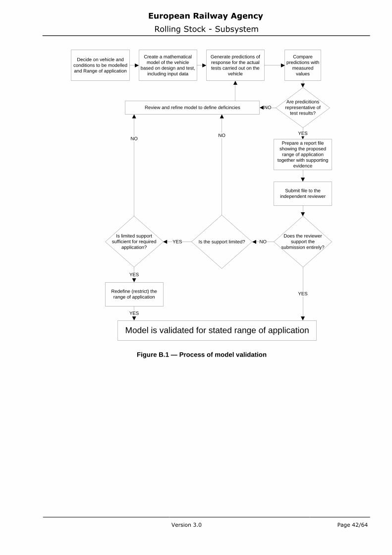
European Railway Agency
Rolling Stock - Subsystem
Version 3.0 Page 42/64
Decide on vehicle and
conditions to be modelled
and Range of application
Create a mathematical
model of the vehicle
based on design and test,
including input data
Generate predictions of
response for the actual
tests carried out on the
vehicle
Compare
predictions with
measured
values
Are predicitions
representative of
test results?
Review and refine model to define deficincies NO
Prepare a report file
showing the proposed
range of application
together with supporting
evidence
YES
Submit file to the
independent reviewer
Does the reviewer
support the
submission entirely?Is the support limited?
Is limited support
sufficient for required
application?
NOYES
NONO
YES
Redefine (restrict) the
range of application
Model is validated for stated range of application
YES
YES
Figure B.1 — Process of model validation
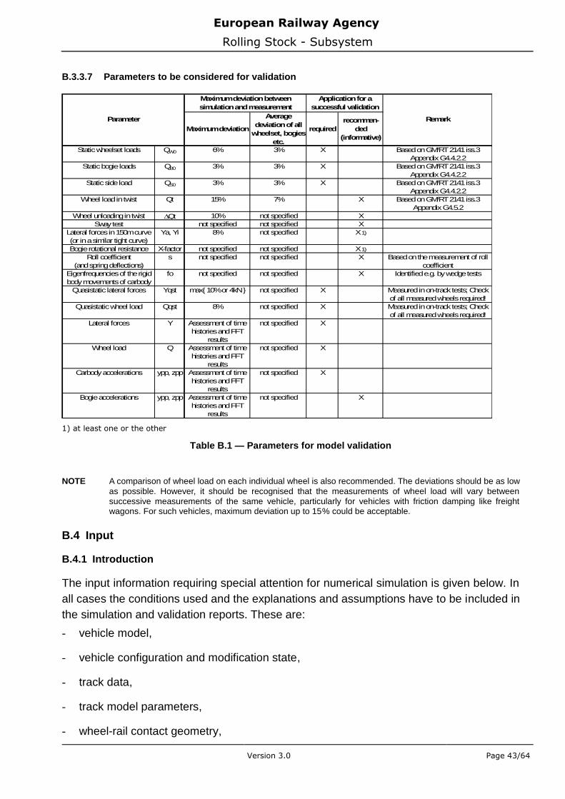
European Railway Agency
Rolling Stock - Subsystem
Version 3.0 Page 43/64
B.3.3.7 Parameters to be considered for validation
Maximum deviation
Average
deviation of all
wheelset, bogies
etc.
required
recommen-
ded
(informative)
Static wheelset loads QW0 6% 3% X Based on GM/RT 2141 iss.3
Appendix G4.4.2.2
Static bogie loads QB0 3% 3% X Based on GM/RT 2141 iss.3
Appendix G4.4.2.2
Static side load QS0 3% 3% X Based on GM/RT 2141 iss.3
Appendix G4.4.2.2
Wheel load in twist Qt 15% 7% X Based on GM/RT 2141 iss.3
Appendix G4.5.2
Wheel unloading in twist Qt 10% not specified X
Sway test not specified not specified X
Lateral forces in 150m curve
(or in a similar tight curve)
Ya, Yi 8% not specified X 1)
Bogie rotational resistance X-factor not specified not specified X 1)
Roll coefficient
(and spring deflections)
s not specified not specified X Based on the measurement of roll
coefficient
Eigenfrequencies of the rigid
body movements of carbody
fo not specified not specified X Identified e.g. by wedge tests
Quasistatic lateral forces Yqst max{ 10% or 4kN } not specified X Measured in on-track tests; Check
of all measured wheels required!
Quasistatic wheel load Qqst 8% not specified X Measured in on-track tests; Check
of all measured wheels required!
Lateral forces Y Assessment of time
histories and FFT
results
not specified X
Wheel load Q Assessment of time
histories and FFT
results
not specified X
Carbody accelerations ypp, zpp Assessment of time
histories and FFT
results
not specified X
Bogie accelerations ypp, zpp Assessment of time
histories and FFT
results
not specified X
Application for a
successful validation
Remark
Maximum deviation between
simulation and measurement
Parameter
1) at least one or the other
Table B.1 — Parameters for model validation
NOTE A comparison of wheel load on each individual wheel is also recommended. The deviations should be as low
as possible. However, it should be recognised that the measurements of wheel load will vary between
successive measurements of the same vehicle, particularly for vehicles with friction damping like freight wagons. For such vehicles, maximum deviation up to 15 % could be acceptable.
B.4 Input
B.4.1 Introduction
The input information requiring special attention for numerical simulation is given below. In
all cases the conditions used and the explanations and assumptions have to be included in
the simulation and validation reports. These are:
- vehicle model,
- vehicle configuration and modification state,
- track data,
- track model parameters,
- wheel-rail contact geometry,

European Railway Agency
Rolling Stock - Subsystem
Version 3.0 Page 44/64
- rail surface condition (friction coefficient),
- direction of travel,
- speed,
- position of the vehicle in the trainset,
- tractive effort, hauled or on its own power, as per on-track test.
The following sub-clauses consider these in more detail.
B.4.2 Vehicle model
A vehicle model has to be a correct representation of all the aspects of the actual vehicle
that influence the dynamic behaviour. This requires a full 3-dimensional non-linear model
of the vehicle which includes:
- masses, inertias and load distribution,
- suspension stiffness, damping, friction, bump-stops etc.,
- wheel-rail interface characteristics,
- when necessary, flexibility of the vehicle body or bogie structure.
B.4.3 Vehicle configuration
The vehicle configuration, load condition, etc. for the numerical simulation has to be in
accordance with the configuration used for testing.
B.4.4 Track data
B.4.4.1 Introduction
In order to carry out numerical simulations of the vehicle dynamic behaviour the track data
must be suitable for use in simulations. This chapter contains the requirements for the
track data to be used and the processing requirements of that data.
B.4.4.2 Source of track data
It is not permitted to use the same track section for both tests and simulations in the
statistical analysis. The combined track sections for each test zone from tests and
simulations, or from simulations alone, have to meet the requirements of EN 14363:2005
including amendments in this document.
A minimum number of 15 track sections for each test zone have to be obtained from on-
track tests.
- The track data that is used must originate from measurements of actual track.
- The measurement of the track data have to be performed with one of the measuring systems defined in EN 13848-2:2006.

European Railway Agency
Rolling Stock - Subsystem
Version 3.0 Page 45/64
- The track measurement accuracy, after transfer function filtering (if required), has to be in accordance with the requirements in EN 13848-1:2003+A1:2008.
NOTE The track recording accuracy and resolution as specified in EN 13848-1:2003+A1:2008 may not be sufficient
for simulation purposes, especially for validation. A measurement uncertainty of 0.5 mm or better is
recommended.
B.4.4.3 Characteristics of track data
- The location of track data must be identified.
- For the validation of the model the track data must comply with the requirements in B.3.3.4.1.
- For the vehicle acceptance the track data must satisfy the requirements of this leaflet as stated in Annex C of EN 14363:2005 and must reflect a naturally existing distribution.
- The track data must represent the true three dimensional record of track, including vertical alignment, cross level, lateral alignment and track gauge.
- The phase relationship of all track data parameters has to be maintained to replicate the actual track data.
- The wavelength range of the measured track irregularity data, when taken in combination with the vehicle speed, should at least correspond to excitation frequencies of the vehicle over the range of 0.4 Hz to 20 Hz for all test zones.
NOTE It is understood that the wavelength contents of recorded track data is often limited but this is not permitted
for simulations. In particular, although the required TL90 and TL100 values are calculated on the 3 m to 25 m wavelength band, this is not sufficient for use in simulations.
B.4.4.4 Processing and editing of track data
- The processed track data must represent the true magnitudes of the actual measured track.
- There must not be any distortion of the data arising from the measuring system or the subsequent processing of the data when compared to the actual track data.
- It is permissible to separate the measured design geometry from the measured track irregularity when creating a track file. The re-combination of the data must not change any characteristics of the representation of the track by change of phase relationship, duplication of data or any other means.
- The processing and editing applied to the track data must be described in the simulation report.
B.4.5 Track model parameters
The track stiffness and damping properties used in the simulations have to be
representative of practical conditions.
NOTE Recognised values from literature or experience from the past may be used.

European Railway Agency
Rolling Stock - Subsystem
Version 3.0 Page 46/64
B.4.6 Wheel-rail contact geometry
A range of rail profiles has to be used for the numerical simulations. The rail profiles have
to be selected to cover the range expected during running on the proposed routes and to
represent the distribution of profiles from new to worn rail. The profiles used for particular
track sections have to be appropriate to those sections (for example: high speed tangent
track or very small radius curves).
The wheel profiles used for the numerical simulations have to be appropriate for the
vehicle being assessed. These may be new wheel profiles or they may represent a wheel
profile worn in service.
The wheel-rail contact conditions have to be consistent with the range of conditions that
would be encountered during testing.
B.4.7 Rail surface condition
For a test on track there will be a natural variation in the wheel-rail friction conditions,
whilst respecting the condition for dry rails. For numerical simulations some variation is
required to avoid the possibility of the results being distorted by use of a single value. The
range and distribution used must be justified in the simulation and/or validation reports.
It is essential that the condition of dry rails is represented and therefore the wheel-rail
friction has to be at least 0.36.
NOTE From measurements made by British Railways the following distribution was observed: Single sided normal
distribution from 0.36 with standard deviation of 0.075. An example for a distribution of a total of 102
sections with 5 different values for the friction coefficient can be seen in the following diagram:
0.35 0.4 0.45 0.5 0.55 0.60
5
10
15
20
25
30
35
40
45
50
friction coefficient
num
ber
of
sections p
er
consta
nt
fric
tion
total number of sections: 102
mue = 0.36
sigma = 0.075
0.3
6
0.4
2
0.4
7
0.5
3
0.5
8
Figure B.2 — Example for the distribution of the friction coefficient
B.4.8 Direction of travel
For the case of a symmetrical vehicle, all necessary assessment values can be obtained
for all required positions from the same simulation and so there is no requirement to
reverse the direction of travel.
If the vehicle being assessed is significantly asymmetric then the numerical simulations
have to be carried out with the vehicle in both directions of travel to determine the worst
condition for each assessment value.
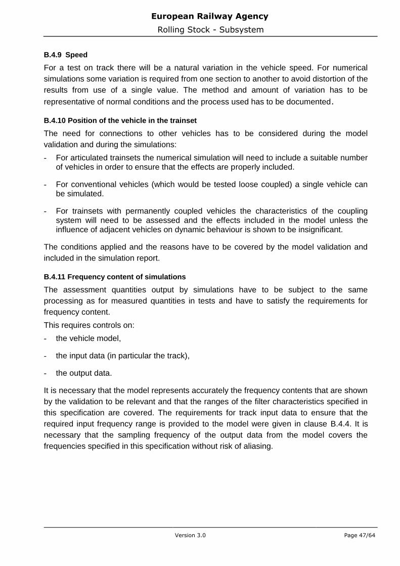
European Railway Agency
Rolling Stock - Subsystem
Version 3.0 Page 47/64
B.4.9 Speed
For a test on track there will be a natural variation in the vehicle speed. For numerical
simulations some variation is required from one section to another to avoid distortion of the
results from use of a single value. The method and amount of variation has to be
representative of normal conditions and the process used has to be documented.
B.4.10 Position of the vehicle in the trainset
The need for connections to other vehicles has to be considered during the model
validation and during the simulations:
- For articulated trainsets the numerical simulation will need to include a suitable number of vehicles in order to ensure that the effects are properly included.
- For conventional vehicles (which would be tested loose coupled) a single vehicle can be simulated.
- For trainsets with permanently coupled vehicles the characteristics of the coupling system will need to be assessed and the effects included in the model unless the influence of adjacent vehicles on dynamic behaviour is shown to be insignificant.
The conditions applied and the reasons have to be covered by the model validation and
included in the simulation report.
B.4.11 Frequency content of simulations
The assessment quantities output by simulations have to be subject to the same
processing as for measured quantities in tests and have to satisfy the requirements for
frequency content.
This requires controls on:
- the vehicle model,
- the input data (in particular the track),
- the output data.
It is necessary that the model represents accurately the frequency contents that are shown
by the validation to be relevant and that the ranges of the filter characteristics specified in
this specification are covered. The requirements for track input data to ensure that the
required input frequency range is provided to the model were given in clause B.4.4. It is
necessary that the sampling frequency of the output data from the model covers the
frequencies specified in this specification without risk of aliasing.
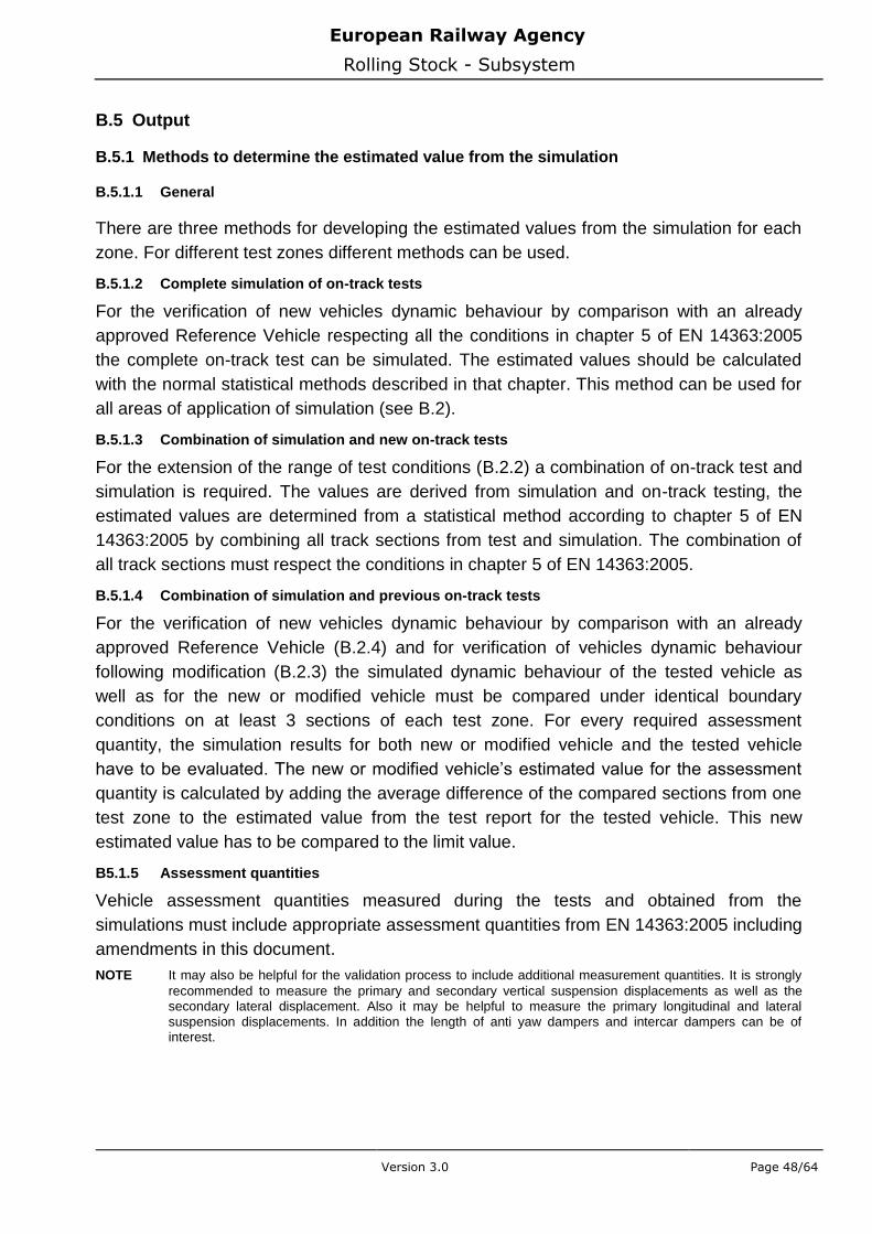
European Railway Agency
Rolling Stock - Subsystem
Version 3.0 Page 48/64
B.5 Output
B.5.1 Methods to determine the estimated value from the simulation
B.5.1.1 General
There are three methods for developing the estimated values from the simulation for each
zone. For different test zones different methods can be used.
B.5.1.2 Complete simulation of on-track tests
For the verification of new vehicles dynamic behaviour by comparison with an already
approved Reference Vehicle respecting all the conditions in chapter 5 of EN 14363:2005
the complete on-track test can be simulated. The estimated values should be calculated
with the normal statistical methods described in that chapter. This method can be used for
all areas of application of simulation (see B.2).
B.5.1.3 Combination of simulation and new on-track tests
For the extension of the range of test conditions (B.2.2) a combination of on-track test and
simulation is required. The values are derived from simulation and on-track testing, the
estimated values are determined from a statistical method according to chapter 5 of EN
14363:2005 by combining all track sections from test and simulation. The combination of
all track sections must respect the conditions in chapter 5 of EN 14363:2005.
B.5.1.4 Combination of simulation and previous on-track tests
For the verification of new vehicles dynamic behaviour by comparison with an already
approved Reference Vehicle (B.2.4) and for verification of vehicles dynamic behaviour
following modification (B.2.3) the simulated dynamic behaviour of the tested vehicle as
well as for the new or modified vehicle must be compared under identical boundary
conditions on at least 3 sections of each test zone. For every required assessment
quantity, the simulation results for both new or modified vehicle and the tested vehicle
have to be evaluated. The new or modified vehicle’s estimated value for the assessment
quantity is calculated by adding the average difference of the compared sections from one
test zone to the estimated value from the test report for the tested vehicle. This new
estimated value has to be compared to the limit value.
B5.1.5 Assessment quantities
Vehicle assessment quantities measured during the tests and obtained from the
simulations must include appropriate assessment quantities from EN 14363:2005 including
amendments in this document.
NOTE It may also be helpful for the validation process to include additional measurement quantities. It is strongly
recommended to measure the primary and secondary vertical suspension displacements as well as the secondary lateral displacement. Also it may be helpful to measure the primary longitudinal and lateral
suspension displacements. In addition the length of anti yaw dampers and intercar dampers can be of interest.

European Railway Agency
Rolling Stock - Subsystem
Version 3.0 Page 49/64
B.6 Report
The outcome of the simulations must be reported together with the other results for the
vehicle in an integrated manner. The report must include the validation report (B.3.3.5).
B.7 Examples for model validation (recommended only)
The following diagrams are included to give examples of comparisons between test results
and simulations. Some of them show good agreement, others illustrate some of the
difficulties that may be encountered.
-30
-20
-10
0
10
20
30
-4 -3 -2 -1 0 1 2 3 4
rotation angle [°]
torq
ue [
kN
m]
Measurement bogy I
Measurement bogy II
Simulation
Figure B.3 — Example comparison for bogie rotation test
Figure B.3 shows an example of the comparison between measurement and simulations
for a bogie rotation test. There are two test results and the simulation. The simulation is a
very good fit with the test results showing a good match of the rotation angle, the torque
values and the suspension behaviour at the ends of the hysteresis loop.
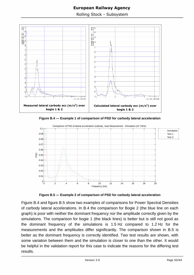
European Railway Agency
Rolling Stock - Subsystem
Version 3.0 Page 50/64
Measured lateral carbody acc (m/s2) over
bogie 1 & 2
Calculated lateral carbody acc (m/s2) over
bogie 1 & 2
Figure B.4 — Example 1 of comparison of PSD for carbody lateral acceleration
0 2 4 6 8 10 12 14 16 18 200
0.01
0.02
0.03
0.04
0.05
0.06
0.07
0.08
0.09
0.1
Frequency [Hz]
PS
D
Comparison of PSD of lateral acceleration (carbody, rear) Measurement - Simulation (LP 10Hz)
Simulation
Test 1
Test 2
Figure B.5 — Example 2 of comparison of PSD for carbody lateral acceleration
Figure B.4 and figure B.5 show two examples of comparisons for Power Spectral Densities
of carbody lateral accelerations. In B.4 the comparison for Bogie 2 (the blue line on each
graph) is poor with neither the dominant frequency nor the amplitude correctly given by the
simulations. The comparison for bogie 1 (the black lines) is better but is still not good as
the dominant frequency of the simulations is 1.5 Hz compared to 1.2 Hz for the
measurements and the amplitudes differ significantly. The comparison shown in B.5 is
better as the dominant frequency is correctly identified. Two test results are shown, with
some variation between them and the simulation is closer to one than the other. It would
be helpful in the validation report for this case to indicate the reasons for the differing test
results.

European Railway Agency
Rolling Stock - Subsystem
Version 3.0 Page 51/64
Measu
red
Y_
20
Hz (
kN
)
Calc
ula
ted
Y_
20
Hz
(kN
)
Figure B.6 — Example of comparison of time history for Y force
Figure B.6 gives an example of a time history comparison for the Y-forces through two
curves, the two black lines should be compared with each other and similarly the two blue
lines. There are some differences between the mean values and it would be helpful to see
explanations for this in the validation report (for example: offsets in the measuring
systems, lack of detailed rail profile measurements). However the dynamic frequencies
and the locations and magnitudes of discrete events are well predicted and this gives
confidence in the validity of the model.
1000 2000 3000 4000 5000 6000-3
-2
-1
0
1
2
3
late
ral a
ccel
erat
ion
[m/s
²]
Comparison of lateral acceleration (carbody, front) Measurement - Simulation (LP 10Hz)
Simulation
Test 1
Test 2
1000 2000 3000 4000 5000 6000-3
-2
-1
0
1
2
3
Distance [m]
late
ral a
ccel
erat
ion
[m/s
²]
Comparison of statistical values (mean, 0.15% and 99.85%)
Simulation
Test 1
Test 2
Time (s)
European Railway Agency
Rolling Stock - Subsystem
Version 3.0 Page 52/64
Figure B.7 — Example of comparison of time history for carbody acceleration
Figure B.7 shows an example of a time history comparison for lateral carbody
acceleration. The presentation is very helpful in showing in the upper graph the time
history trace and, in the lower graph, the mean, 0.15 % and 99.85 % statistics in sections.
This allows the reviewer to assess the comparison more easily than only through the time
history plots where the general levels are difficult to see within the higher frequencies. The
comparison here is good with the mean levels being well predicted and the variations also
in good agreement.
1000 2000 3000 4000 5000 6000 7000 8000-0.2
0
0.2
0.4
0.6
0.8
1
1.2
Y/Q
(2m
slid
ing m
ean)
Comparison of Y/Q (WS1, right) Measurement - Simulation (LP 20Hz)
Simulation
Test 1
Test 2
1000 2000 3000 4000 5000 6000 7000 8000-0.2
0
0.2
0.4
0.6
0.8
1
1.2
Distance [m]
Y/Q
(2m
slid
ing m
ean)
Comparison of statistical values (mean, 0.15% and 99.85%)
Simulation
Test 1
Test 2
Figure B.8 — Example of comparison of time history for Y/Q
Figure B.8 uses the same style of presentation as B.7 and here it is clear that the
comparison is poor. The mean levels are not well represented and the 0.15 % or 99.85 %
values are very different. The time history plot also shows these differences but it is more
difficult to determine.
Time (s)

European Railway Agency
Rolling Stock - Subsystem
Version 3.0 Page 53/64
Q_20 Hz guiding wheel (mean, 99.85%), measured & calculated (nominal)
0
50
100
150
200
meas R1
(-297 m)
calc nom
case R1
meas R2
(453 m)
calc nom
case R2
meas R3
(-595 m)
calc nom
case R3
meas R4
(300 m)
calc nom
case R4
Q_20 H
z (
kN
)
Figure B.9 — Example of comparison of processed data for Q forces
Figure B.9 shows an example of the comparison of statistical results for Q-force on a
number of different curves. The comparison is good with both the mean values and the
99.85 % levels giving similar values for measurement and simulation.
0 0.02 0.04 0.06 0.08 0.1 0.12 0.14 0.16 0.18 0 20 40 60 80
100 120 140 160 180 Rm: 1381m
Limit Value: 157kN
Q3
a [kN
]
I [m]
P=99.85%-Value LP: 20 Hz N: 54
Xn: 3 QN1: 7 (14%) QN2: 16 (31%) QN3: 28 (55%) >QN3: 0 ( 0%)
115.38kN
Simulation
0 0.02 0.04 0.06 0.08 0.1 0.12 0.14 0.16 0.18 0 20 40 60 80
100 120 140 160 180 Rm: 1381m
Limit Value: 157kN
Q3
a [kN
]
I [m]
P=99.85%-Value LP: 20 Hz N: 54
Xn: 3 QN1: 7 (14%) QN2: 16 (31%) QN3: 28 (55%) >QN3: 0 ( 0%)
115.18kN
Measurement
Figure B.10 — Example for distribution plot of track loading Q
Figure B.10 shows an example for a distribution plot of wheel load over cant deficiency
including a two dimensional statistical analysis. The values for the cant deficiency in the
single sections do not match exactly, because the speed in the simulation and the test are
not exactly the same. Although the maximum values for the force of the single sections do
not match exactly, the overall distribution is very similar which results in a similar estimated
value in the statistics.
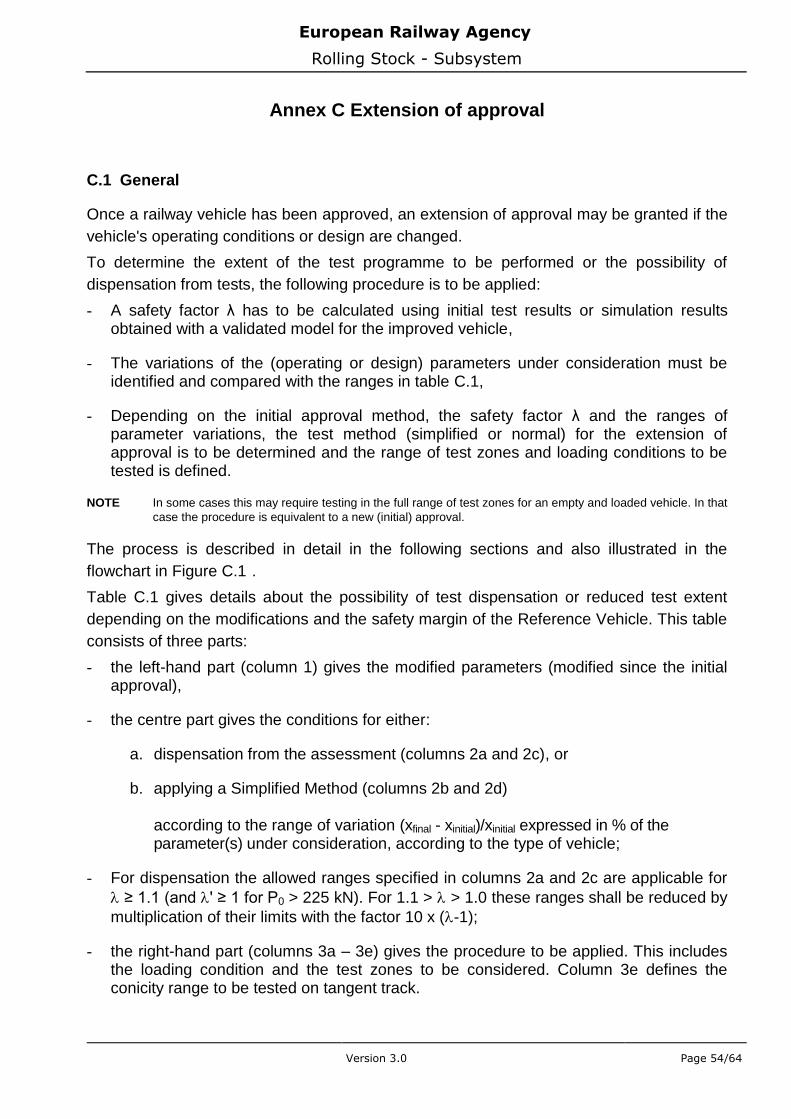
European Railway Agency
Rolling Stock - Subsystem
Version 3.0 Page 54/64
Annex C Extension of approval
C.1 General
Once a railway vehicle has been approved, an extension of approval may be granted if the
vehicle's operating conditions or design are changed.
To determine the extent of the test programme to be performed or the possibility of
dispensation from tests, the following procedure is to be applied:
- A safety factor λ has to be calculated using initial test results or simulation results obtained with a validated model for the improved vehicle,
- The variations of the (operating or design) parameters under consideration must be identified and compared with the ranges in table C.1,
- Depending on the initial approval method, the safety factor λ and the ranges of parameter variations, the test method (simplified or normal) for the extension of approval is to be determined and the range of test zones and loading conditions to be tested is defined.
NOTE In some cases this may require testing in the full range of test zones for an empty and loaded vehicle. In that
case the procedure is equivalent to a new (initial) approval.
The process is described in detail in the following sections and also illustrated in the
flowchart in Figure C.1 .
Table C.1 gives details about the possibility of test dispensation or reduced test extent
depending on the modifications and the safety margin of the Reference Vehicle. This table
consists of three parts:
- the left-hand part (column 1) gives the modified parameters (modified since the initial approval),
- the centre part gives the conditions for either:
a. dispensation from the assessment (columns 2a and 2c), or
b. applying a Simplified Method (columns 2b and 2d) according to the range of variation (xfinal - xinitial)/xinitial expressed in % of the parameter(s) under consideration, according to the type of vehicle;
- For dispensation the allowed ranges specified in columns 2a and 2c are applicable for
≥ 1.1 (and ' ≥ 1 for P0 > 225 kN). For 1.1 > > 1.0 these ranges shall be reduced by
multiplication of their limits with the factor 10 x (-1);
- the right-hand part (columns 3a – 3e) gives the procedure to be applied. This includes the loading condition and the test zones to be considered. Column 3e defines the conicity range to be tested on tangent track.

European Railway Agency
Rolling Stock - Subsystem
Version 3.0 Page 55/64
If parameters that can influence the running behaviour, which are not included in table C.1,
are changed, it shall be demonstrated (by calculation or other means) that the influence is
favourable or insignificant. If this is not possible on-track tests shall be carried out, the
extent of which shall be established according to the expected influences of the changes
on the vehicle's behaviour.
Figure C.1 : Flowchart to determine the minimum requirement for the measuring method
C.3
C.4
C.5
C.5

European Railway Agency
Rolling Stock - Subsystem
Version 3.0 Page 56/64
1 2a 2b 2c 2d 3a 3b 3d 3e
Modified Parameter Applicable range of parameter change Test extent required
Locomotives multiple units
passenger coaches Freight stock
for test dispensa
tion
for testing with a
simplified
measuring
methodk
for test dispensa
tion
for testing with a
simplified
measuring
methodk
Str
aig
ht
track
Zo
ne
1
La
rge-r
ad
ius
cu
rves
Zo
ne
2
Sm
all a
nd
very
sm
all-r
ad
ius
cu
rves
Zo
ne
3,
4
Co
nic
ity r
an
ge
to
be
teste
d n
)
Operational parameters
Increase of permissible maximum speed m --
c
0km/h to 10km/h
--c
not applicab
le
Empty
Empty
- 1)
10km/h to
20km/h (H-
Forces required)
0km/h to
20km/h (H-
Forces required above
10km/h)
Empty
Loaded
Empty
Loaded
- 1)
Increase of permissible cant deficiency --c --
b --
c --
b - - - -
Vehicle parameters
Distance between bogie centres for 2a*>9m e
not applicable
not applicabl
e
-15% to +A
a
-30% to +A
a
Empty
- - 3)
Distance between bogie centres for 2a*<9m e
-5% to +A
a
-10% to +A
a
Empty
- - 3)
Distance between bogie centres general -5% to 20%
-10% to +A
a
not applicable
not applicab
le
Empty
- Empt
y o
3)
Vehicle wheel base (non bogie vehicle) for 2a*>=8m
e not
applicable
not applicabl
e
-15% to +A
a
-30% to +A
a Empt
y - - 1)
Vehicle wheel base (non bogie vehicle) for 2a*<8m
e
-5% to +A
a
-10% to +A
a
Virtual position of centre of gravity i
-20% to 10%
-40% to 20%
not applicable
not applicab
le
Empty
Empty
- 4)
Centre of gravity height - empty vehicle, hg j
-20% to 10%
-40% to 40%
-100% to 20%
-100% to Aa
Empty
Empty
- 3)
Centre of gravity height - loaded vehicle, hg j
-20% to 10%
-40% to 40%
-100% to 50%
-100% to Aa
Loaded
Loaded
- 3)
Centre of gravity height - loaded vehicle g, h
, not
applicable
not applicabl
e
-100% to
0,8('-1) .100%
-100% to
0,8('-1) .100%
Loaded
Loaded
Loaded
3)
Moment of inertia around z-axis of vehicle body (bogie vehicles)
-10% to 10%
-10% to 10%
-10% to 10%
-10% to 10%
Empty
Loaded
Empty
Loaded
Empty
Loaded
2) if <-
10% 3) if >10%
Moment of inertia around z-axis of vehicle body (non bogie vehicle)
not applicable
not applicabl
e
-100% to 10%
-100% to 20%
d
(H-Forces
required above 10%)
Empty
- -
2) if <-
10% 3) if >10%
Vehicle tare for vehicles with tare mass >= 12t (non-bogie wagons) or >= 16t (bogie wagons)
f
not applicable
not applicabl
e
-15% to +A
a
-30% to +A
a
Empty
- - 2)
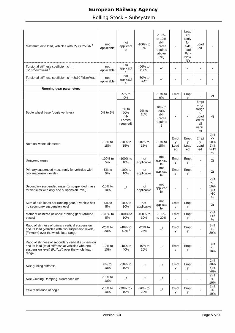
European Railway Agency
Rolling Stock - Subsystem
Version 3.0 Page 57/64
Maximum axle load, vehicles with P0 <= 250kN f
not applicable
not applicabl
e
-100% to 5%
-100% to 10%
(H-Forces
required above 5%)
-
Loaded
(only for
axle load P0 > 225kN
f)
Loaded
-
Torsional stiffness coefficient ct* <=
3x10¹⁰
kNm²/rad e
not applicable
not applicabl
e
-66% to 200%
--b - - - -
Torsional stiffness coefficient ct* > 3x10
10kNm²/rad
e
not applicable
not applicabl
e
-50% to +A
a
--b - - - -
Running gear parameters
Bogie wheel base (bogie vehicles) 0% to 5%
-5% to 0%
0% to 10%
-10% to 0%
Empty
Empty
- 2)
5% to 20% (H-
Forces required)
10% to 20% (H-
Forces required
)
- -
Empty for freigh
t, Loaded for
all vehicl
es
4)
Nominal wheel diameter -10% to
15% -10% to
15% -10% to
15% -10% to
15%
Empty
Loaded
Empty
Loaded
Empty
Loaded
2) if <-
10% 3) if
>+15%
Unsprung mass -100% to
5% -100% to
10% not
applicable
not applicab
le
Empty
Empty
- 2)
Primary suspended mass (only for vehicles with two suspension levels)
-5% to 5%
-10% to 10%
not applicable
not applicab
le
Empty
Empty
- 2)
Secondary suspended mass (or suspended mass for vehicles with only one suspension level)
-10% to 10%
--b
not applicable
not applicab
le - - -
2) if <-
10% 3) if >10%
Sum of axle loads per running gear, if vehicle has no secondary suspension level
-5% to 5%
-10% to 10%
not applicable
not applicab
le
Empty
Empty
- 2)
Moment of inertia of whole running gear (around z-axis)
-100% to 5%
-100% to 10%
-100% to 10%
-100% to 20%
Empty
Empty
- 2) if >+5%
Ratio of stiffness of primary vertical suspension and its load (vehicles with two suspension levels) (Fz+/cz+) over the whole load range
-20% to 20%
-40% to 40%
j
-20% to 25%
--b
Empty
Empty
- 3) if < -
20%
Ratio of stiffness of secondary vertical suspension and its load (total stiffness at vehicles with one suspension level) (Fz*/cz*) over the whole load range
-10% to 10%
-40% to 40%
-10% to 25%
--b
Empty
Empty
- 3) if < -
10%
Axle guiding stiffness 0% to 10%
-10% to 10%
--c --
b
Empty
Empty
-
2) if <0% 4) if >0%
Axle Guiding Damping, clearences etc. -10% to
10% --
b --
c --
b - - -
2) if <-
10%
Yaw resistance of bogie -10% to
10% -20% to -
10% -20% to
20% --
b
Empty
Empty
- 2) if <-
10%
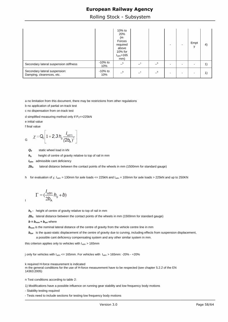
European Railway Agency
Rolling Stock - Subsystem
Version 3.0 Page 58/64
10% to 20% (H-
Forces required above
10% for Iadm>165
mm)
- - Empt
y 4)
Secondary lateral suspension stiffness -10% to
10% --
b --
c --
b - - - 1)
Secondary lateral suspension: Damping, clearences, etc.
-10% to 10%
--b --
c --
b - - - 1)
a no limitation from this document, there may be restrictions from other regulations b no application of partial on-track test
c no dispensation from on-track test
d simplified measuring method only if P0<=225kN e initial value f final value
G
Q0 static wheel load in kN hg height of centre of gravity relative to top of rail in mm
Iadm admissible cant deficiency 2bA lateral distance between the contact points of the wheels in mm (1500mm for standard gauge)
h for evaluation of : Iadm = 130mm for axle loads <= 225kN and Iadm = 100mm for axle loads > 225kN and up to 250KN
I
hg - height of centre of gravity relative to top of rail in mm
2bA lateral distance between the contact points of the wheels in mm (1500mm for standard gauge) b = bnom + bqst where
bnom is the nominal lateral distance of the centre of gravity from the vehicle centre line in mm bqst is the quasi-static displacement of the centre of gravity due to curving, including effects from suspension displacement,
a possible cant deficiency compensating system and any other similar system in mm.
this criterion applies only to vehicles with Iadm > 165mm
j only for vehicles with Iadm <= 165mm. For vehicles with Iadm > 165mm: -20% - +20%
k required H-force measurement is indicated
m the general conditions for the use of H-force measurement have to be respected (see chapter 5.2.2 of the EN 14363:2005)
n Test conditions according to table 2:
1) Modifications have a possible influence on running gear stability and low frequency body motions
- Stability testing required - Tests need to include sections for testing low frequency body motions

European Railway Agency
Rolling Stock - Subsystem
Version 3.0 Page 59/64
2) Modifications have a possible influence only on running gear stability - Stability testing required
3) Modifications have a possible influence only on low frequency body motions: Testing has to include track sections with
- Tests need to include sections for testing low frequency body motions 4) Modifications have no influence on running gear stability and low frequency body motions
- No specific requirements for contact geometry apply
o only if modification is greater than +20% and Iadm >=165mm
Table C.1 – Parameter change table
C.2 Determination of the safety factor
The safety factor is defined as the minimum value obtained from all of the ratios
"(limit value) / (estimated maximum value)" of running safety assessment quantities
(as appropriate for the chosen measuring method) separately evaluated for each loading
condition, test zone.
The factor ' is defined for vehicles with P0 > 225 kN as the minimum value obtained from
all of the ratios "(limit value) / (estimated value)" of track loading assessment quantities
Q and Qqst separately evaluated for each test zone.
The safety factor is to be evaluated only for normal operating conditions, not for fault
modes.
If the initial acceptance has not been done with the method of this document the safety
factor shall be determined and the method used shall be documented. The original
acceptance tests shall comply in principle with the relevant requirements of EN
14363:2005.
C.3 Dispensation
C.3.1 General
Dispensation from testing is given, if all parameter variations fall within the ranges in the
column 2a or 2c of table C.1, possibly reduced as specified in C.1. Otherwise a partial or
full on-track test has to be performed.
C.3.2 Special cases
If the following conditions are fulfilled, deviating from the conditions for test dispensation
for a vehicle laid down in clause C.3.1, the variations of a parameter may be doubled in
the range between the values characterising two already tested vehicles, when such an
extension covers the whole range (see figure C.2) :
1. The vehicle has to be of the same family or design concept as the tested vehicles (in all aspects that influence the dynamic performance).
2. At least two vehicles have to be tested and approved according to EN 14363:2005.

European Railway Agency
Rolling Stock - Subsystem
Version 3.0 Page 60/64
3. The tested vehicles have to be selected in a way that they are representative for the boundaries of the expected test results, e.g. the lightest and heaviest vehicle in a multiple unit.
Figure C.2 – extension of parameter range where : a = value of parameter in question for first vehicle b = value of parameter in question for second vehicle x,x’ = lower percentage of allowed range for parameter change y, y’ = upper percentage of allowed range for parameter change For a < b the condition a(1+2y) ≥ b(1-2x') shall be fulfilled It is possible to approve a third vehicle, if acceleration measurements according to the Simplified Method are performed and the level of acceleration is comparable to the acceleration level of the vehicles approved with the Normal Method. In this case the vehicle to be approved has to be in the same test train as the vehicles tested with the Normal Method. The above conditions 1) and 3) also apply.
C.4 Check for base conditions for Simplified Method
When a test is required, and provided that after the parameter change(s) the base
conditions for a Simplified Method are fulfilled, such a method can be applied for the cases
stated in columns 3a - 3d for the modified parameters, even if the parameter changes are
outside the limits of columns 2b or 2d. H-forces shall be measured if required by the base
conditions for H-force measurement.
C.5 Requirements depending on the initial approval
Only if the base conditions for applying a Simplified Method are not fulfilled, the procedure
to be applied depends on the initial approval. A Simplified Method can still be applied, if all
of the following conditions are fulfilled:
- the initial approval was based on the Normal Method,
- all parameter variations are inside the ranges of table C.1, columns 2b and 2d, possibly
reduced as specified in table C.1 for ≥ 1.1.
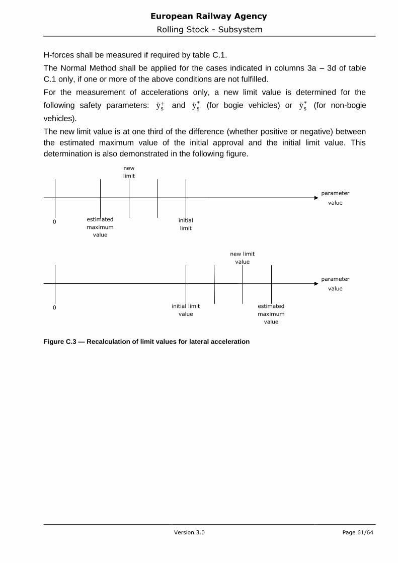
European Railway Agency
Rolling Stock - Subsystem
Version 3.0 Page 61/64
H-forces shall be measured if required by table C.1.
The Normal Method shall be applied for the cases indicated in columns 3a – 3d of table
C.1 only, if one or more of the above conditions are not fulfilled.
For the measurement of accelerations only, a new limit value is determined for the
following safety parameters: ys and *ys (for bogie vehicles) or *ys (for non-bogie
vehicles).
The new limit value is at one third of the difference (whether positive or negative) between
the estimated maximum value of the initial approval and the initial limit value. This
determination is also demonstrated in the following figure.
Figure C.3 — Recalculation of limit values for lateral acceleration
0
new limit
value
initial limit
value
parameter
value
estimated
maximum
value
0 estimated
maximum
value
new
limit
value
initial
limit
value
parameter
value
European Railway Agency
Rolling Stock - Subsystem
Version 3.0 Page 62/64
Annex D Evaluation of contact geometry parameters
D.1 Evaluation of equivalent conicity
If required, rail profiles shall be measured (see Annex D.2) and the equivalent conicity
function tane= f(y) described in EN15302:2008+A1:2010 shall be determined.
1. Depending on the track gauge (TG) and the spacing of active faces (SR), the value of
tan e shall be determined for each rail profile for the following amplitude y:
mmSRTGifmmy
mmSRTGmmifSRTG
y
mmSRTGifmmy
5,2
7)(5,2
1)(
7,3
2. The following function shall be determined:
a. sliding mean over 100 m of tane
b. using a step equal to the spacing between rail measurements. The resulting values shall be considered as applying at the mid-point of the 100 m length.
NOTE If a detailed analysis of vehicles behaviour is performed, other values from tane relationship may also be useful.
D.2 Requirements for manual rail profile measurements
D.2.1 General
The manual measurements can be conducted with any measuring system for rail profile
measurements which fulfils the requirements for profile measurements required for
calculation of equivalent conicity according to EN 15302:2008+A1:2010.
The assessment of the contact geometry parameters shall be made for a typical loaded
condition of the track. As manual rail profile measurements are usually carried out on an
unloaded track the possible effect of the loading (for example on rail roll) shall be
assessed and commented in the report. One method to consider the effect of track loading
on the track profile measurement is to carry out the rail profile measurements in the direct
neighbourhood (within a distance of 1 m from the wheelset) of a rail vehicle with typical
axle load which is loading the track.
D.2.2 Measurements for equivalent conicity
Sufficient measurements of the profiles of both rails and the track gauge shall be made to demonstrate that the requirements for Equivalent Conicity are met. The rail profiles of both rails and the track gauge shall be measured at least every 25 m in each of the selected track sections. NOTE This requirement for manual measurement is less demanding than required by the informative Annex I of EN
15302:2008+A1:2010

European Railway Agency
Rolling Stock - Subsystem
Version 3.0 Page 63/64
D.2.3 Automatic measurements
As the accuracy of an individual measurement is often lower for automatic measurements
than for manual measurement, automatic measurements shall be performed with a regular
spacing not exceeding 6 m to improve the confidence.

European Railway Agency
Rolling Stock - Subsystem
Version 3.0 Page 64/64