Interpolation approximations based on Gauss–Lobatto–Legendre–Birkhoff ...lilian/JAT09Birkhoff.pdf · Journal of Approximation Theory 161 (2009) 142–173 Interpolation approximations

Journal of Approximation Theory 161 (2009) 142–173www.elsevier.com/locate/jat

Interpolation approximations based onGauss–Lobatto–Legendre–Birkhoff quadrature

Li-Lian Wanga,∗, Ben-yu Guob,c

a Division of Mathematical Sciences, School of Physical and Mathematical Sciences, Nanyang Technological University(NTU), 637616, Singapore

b Department of Mathematics, Shanghai Normal University, Shanghai, 200234, Chinac Scientific Computing Key Laboratory of Shanghai Universities, Shanghai E-institute for Computational Science, China

Received 30 May 2007; received in revised form 31 July 2008; accepted 7 August 2008Available online 13 November 2008

Communicated by Joseph Szabados

Abstract

We derive in this paper the asymptotic estimates of the nodes and weights of the Gauss–Lobatto–Legendre–Birkhoff (GLLB) quadrature formula, and obtain optimal error estimates for the associated GLLBinterpolation in Jacobi weighted Sobolev spaces. We also present a user-oriented implementation of thepseudospectral methods based on the GLLB quadrature nodes for Neumann problems. This approach allowsan exact imposition of Neumann boundary conditions, and is as efficient as the pseudospectral methodsbased on Gauss–Lobatto quadrature for PDEs with Dirichlet boundary conditions.c© 2008 Elsevier Inc. All rights reserved.

Keywords: GLLB quadrature rule; Collocation method; Neumann problems; Asymptotic estimates; Interpolation errors

1. Introduction

In a recent work, Ezzirani and Guessab [8] proposed a fast algorithm for computingthe nodes and weights of some Gauss–Birkhoff type quadrature formulae (cf. [19,20])with mixed boundary conditions. One special rule of particular importance, termed as the

∗ Corresponding author.E-mail address: [email protected] (L.-L. Wang).

0021-9045/$ - see front matter c© 2008 Elsevier Inc. All rights reserved.doi:10.1016/j.jat.2008.08.016

http://www.elsevier.com/locate/jat

mailto:[email protected]

http://dx.doi.org/10.1016/j.jat.2008.08.016

L.-L. Wang, B.-y. Guo / Journal of Approximation Theory 161 (2009) 142–173 143

Gauss–Lobatto–Legendre–Birkhoff (GLLB) quadrature, takes the form∫ 1

−1φ(x)dx ∼ φ′(−1)ω− +

N−1∑j=1

φ(x j )ω j + φ′(1)ω+, (1.1)

which is exact for all polynomials of degree 2N − 1, and whose interior nodes are zeros of thequasi-orthogonal polynomial (cf. [25]) formed by a linear combination of the Jacobi polynomialsJ (2,2)N−1 (x) and J (2,2)N−3 (x). Motivated by [8], our first intention is to study the asymptotic behaviorsof the nodes and weights of (1.1). Two important results are

x j ∼= cos(2 j + 1/2)π

2N + 1, 1 ≤ j ≤ N − 1, (1.2)

and

ω j ∼=π

Nsin θ j , θ j = arccos x j , 1 ≤ j ≤ N − 1. (1.3)

With the aid of these estimates, we are able to analyze the GLLB interpolation errors:

‖I N u − u‖L2(I ) + N−1‖(1− x2)1/2(I N u − u)′‖L2(I )

≤ cN−m‖(1− x2)(m−2)/2u(m)‖L2(I ), (1.4)

where I = (−1, 1) and I N is the Gauss–Birkhoff interpolation operator associated with theGLLB points. Similar to the approximation results on the Legendre–Gauss–Lobatto interpolationobtained in [15,16], the estimate (1.4) is optimal.

The GLLB quadrature formula involves derivative values φ′(±1) at the endpoints. Henceits nodes can be a natural choice of the preassigned interpolation points for many importantproblems, such as numerical integration and integral equations with the data of derivatives at theendpoints, etc. In particular, it plays an important role in spectral approximations of second-orderelliptic problems with Neumann boundary conditions [8]. As we know, the numerical solutionsof such problems given by the commonly used Galerkin method with any fixed mode N , donot fulfill the Neumann boundary conditions exactly. Thereby, we prefer to collocation methodsoftentimes, whose solutions satisfy the physical boundary conditions. Whereas, in a collocationmethod, a proper choice of the collocation points is crucial in terms of accuracy, stability and easeof treating the boundary conditions (BCs), especially, the treatment of BCs is even more criticaldue to the global feature of spectral method [18,21]. The GLLB collocation approximation takesthe boundary conditions into account in such a way that the resulting collocation systems havediagonal mass matrices, and therefore leads to explicit time discretization for time-dependentproblems [8]. However, like the collocation method based on Gauss–Lobatto points [17,5,2,13,3,24,9], the GLLB differentiation matrices are ill-conditioned. Thus a suitable preconditionediteration solver is preferable in actual computations. We construct in this paper an efficient finite-difference preconditioning for one-dimensional second-order elliptic equations. We also presenta user-oriented implementation and an error analysis of the GLLB pseudospectral methods basedon variational formulations.

The rest of the paper is organized as follows. In Section 2, we introduce the GLLB quadratureformula, and then investigate the asymptotic behaviors of its nodes and weights in Section 3.With the aid of asymptotic estimates and some other approximation results, we are able toanalyze the GLLB interpolation errors in Section 4. We give a user-oriented description of the

144 L.-L. Wang, B.-y. Guo / Journal of Approximation Theory 161 (2009) 142–173

implementation of the GLLB collocation method, and present some illustrative numerical resultsin Section 5. The final section is for some concluding remarks.

2. The GLLB quadrature formula

In this section, we introduce the Gauss–Lobatto–Legendre–Birkhoff quadrature formula.

2.1. Preliminaries

We start with some notations to be used in the subsequent sections.

2.1.1. Notations• Let I := (−1, 1), and χ(x) ∈ L1(I ) be a generic positive weight function defined in I .

For any integer r ≥ 0, the weighted Sobolev space H rχ (I ) is defined as usual with the

inner product, semi-norm and norm denoted by (u, v)r,χ , |v|r,χ and ‖v‖r,χ , respectively.In particular, L2

χ (I ) = H0χ (I ), (u, v)χ = (u, v)0,χ and ‖v‖χ = ‖v‖0,χ . For any real

r > 0, H rχ (I ) and its norm are defined by space interpolation as in Admas [1]. In cases

where no confusion would arise, χ may be dropped from the notations, whenever χ ≡ 1.• Let ωα(x) = (1−x2)α, x ∈ I with α > −1 be the Gegenbauer weight function. In particular,

denote ω(x) = 1− x2.

• Let N be the set of all non-negative integers. For any N ∈ N, let PN be the set of allalgebraic polynomials of degree at most N . Without loss of generality, we assume that N ≥ 4throughout this paper.• Denote by c a generic positive constant, which is independent of any function and N (mode

in series expansion).• For two sequences {zn} and {wn} with wn 6= 0, the expression zn ∼ wn means |zn|/|wn| →

c(6= 0) as n → ∞. In particular, zn ∼= wn means zn/wn ≈ 1 for n � 1, or zn/wn → 1 forn→∞.• For simplicity, we sometimes denote ∂ l

xv =dlvdx l = v

(l), for any integer l ≥ 1.

2.1.2. Jacobi polynomials

We recall some relevant properties of the Jacobi polynomials, denoted by J (α,β)n (x), x ∈ Iwith α, β > −1 and n ≥ 0, which are mutually orthogonal with respect to the Jacobi weightωα,β(x) = (1− x)α(1+ x)β :∫ 1

−1J (α,β)n (x)J (α,β)m (x)ωα,β(x)dx = γ (α,β)n δmn, (2.1)

where δmn is the Knonecker symbol, and

γ (α,β)n =2α+β+1Γ (n + α + 1)Γ (n + β + 1)

(2n + α + β + 1)Γ (n + 1)Γ (n + α + β + 1). (2.2)

In the subsequent discussions, we will mainly use two special types of Jacobi polynomials. Thefirst one is J (2,2)n (x), defined by the three-term recursive relation (see, e.g., Szego [23]):

n(n + 4)J (2,2)n (x) = (n + 2)(2n + 3)x J (2,2)n−1 (x)− (n + 1)(n + 2)J (2,2)n−2 (x),

J (2,2)0 (x) = 1, J (2,2)1 (x) = 3x, x ∈ [−1, 1].(2.3)


The coefficient of leading term of J (2,2)n (x) is

K (2,2)n =

(2n + 4)!2nn!(n + 4)!

. (2.4)

Moreover, we have

J (2,2)n (−x) = (−1)n J (2,2)n (x), J (2,2)n (1) =(n + 1)(n + 2)

2. (2.5)

The corresponding monic polynomial is defined by dividing the leading coefficient in (2.4):

Pn(x) := λn J (2,2)n (x) with λn =

(K (2,2)

n

)−1. (2.6)

As a direct consequence of (2.3) and (2.6),

Pn+1(x) = x Pn(x)− an Pn−1(x) with an =n(n + 4)

(2n + 3)(2n + 5), (2.7)

where P−1 = 0 and P0 = 1. By (2.1)–(2.2), the normalized Jacobi polynomials

Pn(x) := λn J (2,2)n (x) with λn =

(γ (2,2)n

)−1/2, (2.8)

satisfy ‖Pn‖2ω2 = 1.

We will also utilize the Legendre polynomials, denoted by Ln(x), which are mutuallyorthogonal with respect to the unit weight ω = 1. Note that the constant of orthogonality andleading coefficient respectively are

γ (0,0)n = ‖Ln‖2=

22n + 1

, K (0,0)n =

(2n)!

2n(n!)2. (2.9)

Recall that Ln(±1) = (±1)n and L ′n(±1) = 12 (−1)n−1n(n + 1).

2.2. GLLB quadrature formula

The GLLB quadrature formula can be derived from Theorem 4.2 of Ezzirani and Guessab [8],which belongs to a Birkhoff type rule (see, e.g., [19,20]).

Theorem 2.1. Let {Pn} be the monic Jacobi polynomials defined in (2.6). Consider the quasi-orthogonal polynomial:

QN−1(x) = PN−1(x)+ bN PN−3(x), N ≥ 2, (2.10)

where

bN = −(N − 1)(N + 2)(2N 2

+ 2N + 3)

(2N − 1)(2N + 1)(2N 2 − 2N − 3)+

√12(N − 1)(N + 2)(N 2 + N − 3)

(2N − 1)(2N 2 − 2N − 3)

:= −bIN + bIN . (2.11)

Then we have that


¬ For N ≥ 4,

14−

1N< −bN <

(N + 2)(N + 3)(2N − 1)(2N + 1)

. (2.12)

The N−1 zeros of QN−1(x), denoted by{

x j}N−1

j=1 , are distinct, real and all located in (−1, 1).

® There exists a unique set of weights{ω j}N

j=0 such that∫ 1

−1φ(x)dx = φ′(−1)ω0 +

N−1∑j=1

φ(x j )ω j + φ′(1)ωN := S N [φ], ∀φ ∈ P2N−1.(2.13)

¯ The interior weights are all positive and explicitly expressed by

ω j =AN

PN−2(x j )Q′N−1(x j )

1

(1− x2j )

2, 1 ≤ j ≤ N − 1, (2.14)

with

AN =

(1−

bN

aN−2

)λ2

N−2

λ2N−2

, (2.15)

where the constants aN−2, bN , λN−2 and λN−2 are defined in (2.7), (2.11), (2.6) and (2.8),respectively.

Proof. The proof is based on a reassembly and extension of some relevant results in [8]. Forclarity, we first present a one-to-one correspondence between the notations of [8] and those ofthis paper:

ln � N − 1, dσ � (1− x2)2dx, πk � Pk, πk � Pk, qn,2 � QN−1,

βk � ak, sN−1 � bN , βn−1 � aN−2 − bN , J ∗n (σ ) � JN−1.(2.16)

We next derive the expression of bN . By Theorem 4.2 and 4.3 of [8], we find that

aN−2 − bN = βN−2

=−

√12(N − 1)(N + 2)(N 2 + N − 3)+ (N + 2)(2N 2

− 4N + 3)

(2N − 1)(2N 2 − 2N − 3).

Hence, a direct computation leads to

bN = aN−2 − βN−2(2.7)= RHS of (2.11).

¬ The special values b j ( j = 1, 2, 3) can be computed directly via (2.11). To obtain thebounds for bN with N ≥ 4, we first prove that

− bN <(N + 2)(N + 3)(2N − 1)(2N + 1)

. (2.17)

Since −bN = bIN − bIN < bI

N , it suffices to verify

W1 := (N + 2)(N + 3)(2N 2− 2N − 3)− (N − 1)(N + 2)(2N 2

+ 2N + 3) > 0.

A direct calculation yields

W1 = 2(N − 3)(N + 2)(2N + 1).


Hence (2.17) is valid for N ≥ 4, and it remains to prove

− bN >1N−

14. (2.18)

Clearly, −√

N 2 + N − 3 > −√

N 2 + N − 2 = −√(N − 1)(N + 2) and 2N (N − 1) >

2N 2− 2N − 3. Therefore,

−bN >(N − 1)(N + 2)(2N 2

+ 2N + 3)− (2N + 1)√

12(N − 1)(N + 2)

(2N − 1)(2N + 1)(2N 2 − 2N − 3)

>(N − 1)(N + 2)

[(2N 2

+ 2N + 3)− 4(2N + 1)]

(2N − 1)(2N + 1)(2N 2 − 2N − 3)

>(N − 1)(N + 2)(2N 2

− 6N − 8)2N (N − 1)(2N − 1)(2N + 1)

>(N + 2)(N − 4)(N + 1)2N (2N − 1)(2N + 1)

>(N + 2)(N − 4)

2N (2N − 1)>

N − 44N

=14−

1N.

Thus, a combination of (2.17) and (2.18) leads to (2.12). Observe from (2.12) that for N ≥ 3,−bN > 0. Therefore, by Theorem 4.1 of [8], the

quasi-orthogonal polynomial can be expressed as a determinant

QN−1(x) = PN−1(x)+ bN PN−3(x) = det (xIN−1 − JN−1) , (2.19)

where IN−1 is an identity matrix, and JN−1 is a symmetric tri-diagonal matrix of order N − 1,

JN−1 =

0√

a1√a1 0

√a2

. . .. . .

. . .√

aN−3 0√

aN−2 − bN√aN−2 − bN 0

(2.20)

with an and bN given in (2.7) and (2.11), respectively. Therefore, all the zeros of QN−1 are realand distinct.

® Theorem 4.2 of [8] reveals that with such a choice of bN , all the zeros of QN−1 aredistributed in (−1, 1), and the quadrature formula (2.13) is unique. Moreover, the interior weights{ω j }

N−1j=1 are all positive.

¯ We now consider the expressions of the weights. By Formula (38) of [8],

(1− x2j )

2ω j =A∗N

K ∗N (x j ), 1 ≤ j ≤ N − 1, (2.21)

where A∗N = 1− bN/aN−2, and

K ∗N (x j ) = A∗N

N−3∑k=0

P2k (x j )+ P2

N−2(x j ). (2.22)


To simplify K ∗N (x j ), we recall the Christoffel–Darboux formula (see, e.g., Szego [23]):

P ′n+1(x)Pn(x)− P ′n(x)Pn+1(x) =dn+1

dn

n∑k=0

P2k (x) > 0, ∀x ∈ [−1, 1], (2.23)

where dk is the leading coefficient Pk(x), and by (2.6) and (2.8),

dk =λk

λk, Pk(x) = dk Pk(x). (2.24)

Hence,

Q′N−1(x)PN−2(x) −P ′N−2(x)QN−1(x)(2.10)=

[P ′N−1(x)PN−2(x)− P ′N−2(x)PN−1(x)

]− bN

[P ′N−2(x)PN−3(x)− P ′N−3(x)PN−2(x)

](2.24)=

1dN−1

[P ′N−1(x)PN−2(x)− P ′N−2(x)PN−1(x)

]−

bN

dN−3

[P ′N−2(x)PN−3(x)− P ′N−3(x)PN−2(x)

](2.23)=

1dN−2

N−2∑k=0

P2k (x)−

bN dN−2

d2N−3

N−3∑k=0

P2k (x)

=1

dN−2

{[1−

bN d2N−2

d2N−3

]N−3∑k=0

P2k (x)+ P2

N−2(x)

}(2.26)=

1dN−2

{[1−

bN

aN−2

] N−3∑k=0

P2k (x)+ P2

N−2(x)

}.

(2.25)

In the last step, we used the identity

aN−2 =λ2

N−3

λ2N−2

λ2N−2

λ2N−3

=d2

N−3

d2N−2

, (2.26)

which can be verified directly by the definition of the constants. Thus, taking x = x j in (2.25)and using the fact: QN−1(x j ) = 0, 1 ≤ j ≤ N − 1, gives

Q′N−1(x j )PN−2(x j )(2.25)=

1dN−2

{A∗N

N−3∑k=0

P2k (x j )+ P2

N−2(x j )

}=

1dN−2

K ∗N (x j ), (2.27)

which implies that

K ∗N (x j )(2.24)= d2

N−2 Q′N−1(x j )PN−2(x j )(2.24)=

λ2N−2

λ2N−2

Q′N−1(x j )PN−2(x j ).

Plugging it into (2.21) leads to (2.14)–(2.15). �

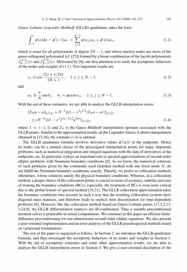
Remark 2.1. ¬ The choice of bN so that all zeros of QN−1(x) are in (−1, 1), is unique, andthereby uniquely determines the quadrature rule. It is seen from (2.12) that bN is uniformlybounded with −bN ∼= 1/4, whose behavior is depicted in Fig. 3.1 (left).

The formulae (2.19)–(2.20) indicate that the quadrature nodes {x j }N−1j=1 are eigenvalues of the

symmetric tridiagonal matrix JN−1, and therefore, can be evaluated by using some standardmethods (e.g., the QR-algorithm) as with the classical Gauss quadrature (see, e.g., [11]).


Fig. 3.1. Left: the constant −bN and its bounds (cf. (2.10)–(2.11)) against N . Right: asymptotic behavior of ∆minN and

∆maxN against N (right).

Making use of Formula (41) of [8], the weights {ω j }N−1j=1 can be computed from the first

component of the orthonormal eigenvectors of JN−1.

® Alternative to the eigen-method, the nodes {x j }N−1j=1 can be located by a root-finding method,

say Newton–Raphson iteration, which turns out to be more efficient for a quadrature rule ofhigher order. A good initial approximation might be {x (0)j }

N−1j=1 given in (3.24). Accordingly,

the weights {ω j }N−1j=1 can be computed via the compact formulae (2.14)–(2.15).

¯ It is worthwhile to point out that the quadrature nodes and weights are symmetric

x j + xN− j = 0, ω j = ωN− j , j = 1, 2, . . . , N − 1. (2.28)

Therefore, the computational cost can be halved.° Let h0 and hN be the Lagrangian polynomials given in (5.6) of this paper. The boundary

weights

ω0 =

∫ 1

−1h0(x)dx, ωN =

∫ 1

−1hN (x)dx .

One verifies that ω0 = −ωN , and an explicit evaluation of the above integrals by using therelevant properties of Jacobi polynomials leads to the formula for ω0 in Theorem 4.2 of [8].

The GLLB quadrature formula (2.13) enjoys the same degree of exactness as theGauss–Legendre–Lobatto (GLL) quadrature (with N + 1 nodes), but in contrast to GLL, GLLBincludes the boundary derivative values φ′(±1), which is thereby suitable for exactly imposingNeumman boundary conditions (see Section 5).

3. Asymptotic properties of the nodes and weights

In this section, we make a quantitative asymptotic estimate of the nodes and weights in theGLLB quadrature formula (2.13). These properties will play an essential role in our subsequentanalysis of the GLLB interpolation errors.

3.1. Asymptotic property of the nodes

We start with the interlacing property. Theorem 4.1 of [20] reveals that the zeros of QN−1interlace with those of QN−2. The following theorem indicates that the zeros of QN−1 also


interlace with those of PN−2, which can be proved in a fashion similar to that in [20]. Forintegrity, we provide the proof below.

Theorem 3.1. Let {x j }N−1j=1 and {yk}

N−2k=1 be the zeros of QN−1(x) and PN−2(x), respectively.

Then we have

− 1 = y0 < x1 < y1 < x2 < y2 < · · · < yN−2 < xN−1 < 1 = yN−1. (3.1)

Proof. We take three steps to complete the proof.Step I: Show that

QN−1(y j )QN−1(y j+1) < 0, j = 1, 2, . . . N − 3, (3.2)

equivalently to say, between two consecutive zeros of PN−2(x), there exists at least one zero ofQN−1(x). To justify this, we first deduce that

Q′N−1(x)PN−2(x)− P ′N−2(x)QN−1(x) > 0, ∀x ∈ [−1, 1], (3.3)

which is a consequence of (2.7), (2.25) and (2.12), since

dN−2 > 0, 1−bN

aN−2> 1+

(14−

1N

)1

aN−2≥ 1, ∀N ≥ 4.

Thanks to PN−2(yk) = 0, taking x = y j , y j+1 in (3.3) yields

P ′N−2(y j )QN−1(y j ) < 0, P ′N−2(y j+1)QN−1(y j+1) < 0, (3.4)

which certainly implies

P ′N−2(y j )P′

N−2(y j+1) · QN−1(y j )QN−1(y j+1) > 0.

Therefore, to prove (3.2), it suffices to check that

P ′N−2(y j )P′

N−2(y j+1) < 0. (3.5)

Notice that

PN−2(x) = dN−2

N−2∏k=1

(x − yk) ,

and consequently,

P ′N−2(y j ) = dN−2

j−1∏k=1

(y j − yk

)·

N−2∏k= j+1

(y j − yk

)= (−1)N− j−2dN−2 · C1,

P ′N−2(y j+1) = (−1)N− j−3dN−2 · C2,

(3.6)

where C1 and C2 are two positive constants. Hence

P ′N−2(y j )P′

N−2(y j+1) = (−1)2N−2 j−5· d2

N−2C1C2 < 0, 1 ≤ j ≤ N − 3. (3.7)

This validates (3.5) and thereby (3.2) follows.Step II: At this point, it remains to consider the possibility of possessing zeros of QN−1(x) insubintervals (yN−2, 1) and (−1, y1). Clearly, by the first identity of (3.6), the largest zero yN−2satisfies P ′N−2(yN−2) > 0. Thus, by (3.4),

QN−1(yN−2) < 0. (3.8)


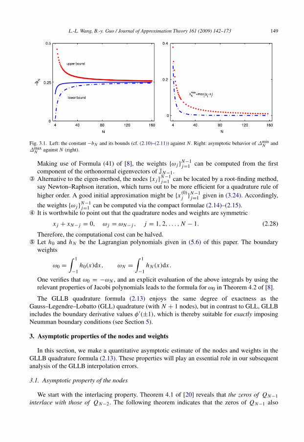
On the other hand, we have

QN−1(1) = PN−1(1)+ bN PN−3(1) > 0, (3.9)

which is due to a direct calculation using (2.5)–(2.6) and (2.12):

PN−1(1)PN−3(1)

+ bN =(N + 2)(N + 3)(2N − 1)(2N + 1)

+ bN > 0,

and PN−3(1) > 0. The sign of (3.8)–(3.9) indicates that there is at least one zero of QN−1(x) inthe interval (yN−2, 1). Using the symmetry of the zeros (see [8,23]):

x j = −xN− j , j = 1, . . . , N − 1; yk = −yN−1−k, k = 1, . . . , N − 2, (3.10)

we deduce that the interval (−1, y1) also contains at least one zero of QN−1(x).

Final step: A combination of the previous statements reaches the conclusion: each of the N − 1subintervals

{(y j , y j+1)

}N−2j=0 (y0 = −1, yN−1 = 1) contains at least one of the N − 1 zeros of

QN−1(x), and therefore there can only be a unique one in each subinterval. �

To visualize the above interlacing property, we denote

∆minN = min

1≤ j≤N−1(y j − x j ), ∆max

N = max1≤ j≤N−1

(y j − x j ), ∀N ≥ 4. (3.11)

According to Theorem 3.1, we expect to see that

∆maxN > ∆min

N > 0, ∀N ≥ 4, limN→∞

∆minN = lim

N→∞∆max

N = 0, (3.12)

which is illustrated by Fig. 3.1(right).In the analysis of interpolation error, we need more precise asymptotic estimates of the GLLB

quadrature nodes. For this purpose, hereafter, we assume that the zeros {x j }N−1j=1 of QN−1(x) are

arranged in descending order. We make the change of variables

x = cos θ, θ ∈ [0, π], θ j = cos−1 x j , j = 1, 2, . . . , N − 1. (3.13)

The main result is stated in the following theorem.

Theorem 3.2. Let{θ j}N−1

j=1 be the same as in (3.13). Then

θ j ∈ I j := (θ j−1, θ j ) ⊂ (0, π), 1 ≤ j ≤ N − 1, (3.14)

where

θ j =2 j + 3

2

2N + 1π, 0 ≤ j ≤ N − 1. (3.15)

In other words,

0 < θ0 < θ1 < θ1 < θ2 < θ2 < · · · < θN−2 < θN−1 < θN−1 < π. (3.16)

Proof. By the intermediate mean-value theorem, (3.14) is equivalent to

QN−1(cos θ j−1)QN−1(cos θ j ) < 0, j = 1, 2, . . . , N − 1. (3.17)


To prove this result, we first recall Formula (8.21.10) of Szego [23]:

J (2,2)n (cos θ) = n−12 G(θ) cos

((n +

52

)θ + γ

)+ O(n−

32 ), θ ∈ (0, π), (3.18)

where

G(θ) = π−12

(sin

θ

2

)− 52(

cosθ

2

)− 52

= 4

√2π(sin θ)−

52 , γ = −

54π. (3.19)

Hence, using (2.6), (2.10) and (3.18) gives

QN−1(cos θ)(2.10)= PN−1(cos θ)+ bN PN−3(cos θ)

(2.6)= λN−1 J (2,2)N−1 (cos θ)+ bNλN−3 J (2,2)N−3 (cos θ)

(3.18)= G(θ)

{(N − 1)−

12 λN−1 cos

((N +

32

)θ + γ

)+ (N − 3)−

12 bNλN−3 cos

((N −

12

)θ + γ

)}+

{λN−1 O((N − 1)−

32 )+ bNλN−3 O((N − 3)−

32 )}

:= HN (θ)+ RN . (3.20)

Notice that θ j in (3.15) solves the equation(N +

12

)θ j + γ =

(j −

12

)π, 0 ≤ j ≤ N − 1,

which implies(N +

32

)θ j + γ =

(j −

12

)π + θ j ,

(N −

12

)θ j + γ =

(j −

12

)π − θ j .

Therefore, taking θ = θ j in (3.20) and using trigonometric identities, gives

HN (θ j ) = G(θ j )

{(N − 1)−

12 λN−1 cos

((j −

12

)π + θ j

)+ (N − 3)−

12 bNλN−3 cos

((j −

12

)π − θ j

)}= (−1) j (sin θ j

)G(θ j )

{(N − 1)−

12 λN−1 − (N − 3)−

12 bNλN−3

}:= (−1) j SN (θ j ). (3.21)

Since −bN > 0, λk > 0 and θ j ∈ (0, π), we have that SN (θ j ) > 0, and thereby

sgn(HN (θ j )

)= (−1) j , 0 ≤ j ≤ N − 1. (3.22)

Moreover, by (2.12), (3.19) and (3.21),

|HN (θ j )| ≥ 252π−

12(sin θ j

)− 32

{(N − 1)−

12 λN−1 +

(14−

1N

)(N − 3)−

12 λN−3

}≥ cN−

12 (λN−1 + λN−3),


Fig. 3.2. Left: the error ∆N (solid line) and N−1.9 (“◦”) against N . Right: asymptotic behavior of δ(1)N (solid line) and

δ(2)N (“◦”) (cf. (3.43)) against N .

which, together with the fact −bN ∼=14 , implies

|RN | ≤ cN−32 (λN−1 + λN−3) ≤ cN−1

|HN (θ j )|. (3.23)

Hence, a combination of (3.20)- (3.23) leads to that

sgn(QN−1(cos θ j )

)= sgn

(HN (θ j )

)= (−1) j , 0 ≤ j ≤ N − 1, ∀N � 1,

which implies (3.17) and therefore, there exists at least one zero of QN−1(cos θ) in eachsubinterval I j = (θ j−1, θ j ), 1 ≤ j ≤ N − 1. Because the number of zeros equals to the numberof subintervals, there exists exactly one zero in I j . �

As a consequence of Theorem 3.2, a good asymptotic approximation to the zeros {x j }N−1j=0

might be

x j = cos θ j ∼= x (0)j := cos

(θ j−1 + θ j

2

)= cos

(2 j + 1/2)π2N + 1

, 1 ≤ j ≤ N − 1. (3.24)

To illustrate this property numerically, we denote

∆N = max1≤ j≤N−1

∣∣∣x j − x (0)j

∣∣∣ .We plot in Fig. 3.2 (left) the error ∆N (solid line) and the reference value N−1.9 (“◦”) against N ,which indicates that ∆N decays algebraically at a rate of N−1.9, and predicts that

x j = cos(2 j + 1/2)π

2N + 1+ O(N−1.9), 1 ≤ j ≤ N − 1. (3.25)

3.2. Asymptotic properties of the weights

We establish below an important result concerning the asymptotic behaviors of the interiorquadrature weights {ω j }

N−1j=1 in (2.13).


Theorem 3.3. Let{θ j}N−1

j=1 be the zeros of the quadrature (trigonometric) polynomialQN−1(cos θ). Then for any N � 1,

ω j ∼=π

Nsin θ j , j = 1, 2, . . . , N − 1. (3.26)

Proof. We rewrite the weights as

ω j(2.14)=

AN

(1− x2j )

2

1PN−2(x j )Q′N−1(x j )

(2.6)=

(2.10)

AN

λN−2λN−3

1

(1− x2j )

2

1

J (2,2)N−2 (x j )W ′N (x j ), (3.27)

where

WN (x) :=λN−1

λN−3J (2,2)N−1 (x)+ bN J (2,2)N−3 (x) = λ

−1N−3 QN−1(x). (3.28)

To prove (3.26), it suffices to study the asymptotic behaviors of the constant, J (2,2)N−2 (x j ) andW ′N (x j ) in (3.27). For clarity, we split the rest of the proof into three steps.Step I: Let us first estimate the constants in (3.27)–(3.28). A direct calculation using (2.6)–(2.7)and (2.12) leads to

aN−2 ∼=14, −bN ∼=

14,

1

λ2N−2

∼=16N,

λN−2

λN−3=(N − 2)(N + 2)

N (2N − 1)∼=

12,

(3.29)

which, together with (2.15), implies

AN

λN−2λN−3=

(1−

bN

aN−2

)λN−2

λN−3λ2N−2

∼=16N. (3.30)

Step II: Let

ΘN , j =

(N +

12

)θ j −

54π. (3.31)

We next show that

sin ΘN , j ∼= 0, ∀N � 1. (3.32)

Since QN−1(x j ) = 0, we have

WN (cos θ j )(3.28)= λ−1

N−3 QN−1(cos θ j ) = λ−1N−3 QN−1(x j ) = 0.

Hence, by (3.18),

0 = WN (cos θ j ) =λN−1

λN−3J (2,2)N−1 (cos θ j )+ bN J (2,2)N−3 (cos θ j )

(3.18)= (N − 3)−

12 G(θ j )

{cN cos

(ΘN , j + θ j

)+ bN cos

(ΘN , j − θ j

)}+ O(N−

32 )

= (N − 3)−12 G(θ j )

{(bN − cN ) sin θ j sin ΘN , j

+ (bN + cN ) cos θ j cos ΘN , j}+ O(N−

32 ),


where G(θ j ) is given in (3.19), and by (3.29),

cN =λN−1

λN−3

(N − 3N − 1

) 12∼=λN−1

λN−2

λN−2

λN−3

∼=14. (3.33)

Consequently,

0 = (bN − cN ) sin θ j sin ΘN , j + (bN + cN ) cos θ j cos ΘN , j + O(N−1 sin5/2 θ j ). (3.34)

On the other hand, using (3.29) and (3.33) leads to

bN + cN ∼= 0, bN − cN ∼= −12, for N � 1. (3.35)

Since sin θ j 6= 0(> 0), the desired result (3.32) follows from (3.34).Step III: Applying Formula (8.8.1) of [23] (note: this formula may be derived by differentiating(3.18) and using (3.28)) to W ′N (x), and using trigonometric identities, yields

dWN

dθ(cos θ j )

= (N − 3)12 G(θ j )

{−cN sin(ΘN , j + θ j )− bN sin(ΘN , j − θ j )+ (N sin θ j )

−1 O(1)}

= (N − 3)12 G(θ j )

{(bN − cN ) sin θ j cos ΘN , j − (bN + cN ) cos θ j sin ΘN , j

+ (N sin θ j )−1 O(1)

}. (3.36)

Hence, by (3.32) and (3.35),

dWN

dθ(cos θ j ) ∼= −

12

√N G(θ j ) sin θ j cos ΘN , j , 1 ≤ j ≤ N − 1, (3.37)

which implies

W ′N (x j ) =dWN

dθ(cos θ j )

dθdx

∣∣∣∣θ=θ j

= −dWN

dθ(cos θ j )

1sin θ j

=

√N

2G(θ j ) cos ΘN , j . (3.38)

On the other hand, by (3.18),

J (2,2)N−2 (cos θ j ) ∼= N−12 G(θ j ) cos ΘN , j , 1 ≤ j ≤ N − 1. (3.39)

Multiplying (3.38) by (3.39) yields

J (2,2)N−2 (x j )W′

N (x j ) ∼=12

G2(θ j ) cos2 ΘN , j ∼=12

G2(θ j ), (3.40)

where in the last step, we used the fact:

cos2 ΘN , j

(3.32)∼= 1, ∀N � 1. (3.41)

Finally, thanks to

1

(1− x2j )

2

(3.13)=

1

sin4 θ j, G2(θ j )

(3.19)=

25

π

1

sin5 θ j,

the desired result (3.26) follows from (3.27), (3.30) and (3.40). �


As a direct consequence of (3.24) and (3.26), we derive the following explicit asymptoticexpression:

ω j ∼= ω(0)j :=

π

Nsin

(2 j + 1/2)π2N + 1

, 1 ≤ j ≤ N − 1. (3.42)

To examine how good it is, we set

δ(1)N =

π

Nmax

1≤ j≤N−1

{sin θ j

ω j

}, δ

(2)N =

π

Nmax

1≤ j≤N−1

{ω(0)j

ω j

}.

By Theorem 3.3, we expect to see that

δ(i)N∼= 1, i = 1, 2, ∀N � 1, (3.43)

which indeed can be visualized from Fig. 3.2(right).So far, we have derived two asymptotic estimates for the GLLB nodes and weights (cf.

(3.24) and (3.42)), which will be useful for the analysis of the GLLB interpolation error in theforthcoming section.

4. GLLB interpolation error estimates

This section is devoted to the analysis of the GLLB interpolation errors in Sobolev norms,which will be used for the error analysis of GLLB pseudospectral methods. We first state the mainresult, and then present the ingredients for the proof including some inequalities and orthogonalprojections. Finally, we give the proof of the interpolation errors.

4.1. The main result

We begin with the definition of the GLLB interpolation operator associated with the GLLBquadrature formula. The GLLB interpolant I N u ∈ PN , satisfies

(I N u)′(±1) = u′(±1), (I N u)(x j ) = u(x j ), 1 ≤ j ≤ N − 1. (4.1)

Denote the weight functions by ω(x) = 1 − x2 and ωα(x) = (1 − x2)α. Let α =max {0,−[α] − 1} with [α] being the largest integer ≤ α. To describe the error, we introducethe weighted Sobolev space

Bmα (I ) :=

{u ∈ L2(I ) : ∂k

x u ∈ L2ωα+k (I ), α + 1 ≤ k ≤ m

}∩ H α(I ), m ≥ 0,

with the norm

‖u‖Bmα (I ) =

(‖u‖2H α(I ) +

m∑k=α+1

‖∂kx u‖2

ωα+k

) 12

.

The main result on the GLLB interpolation error is stated as follows.

Theorem 4.1. For any u ∈ Bm−2(I ) and m ≥ 2,

N‖I N u − u‖ + ‖∂x (I N u − u)‖ω ≤ cN 1−m‖∂m

x u‖ωm−2 . (4.2)


4.2. Preparations for the proof

The main ingredients for the proof Theorem 4.1 consist of the asymptotic estimates (cf.Theorem 3.2 and 3.3), several inequalities and the approximation property of one specificorthogonal projection to be stated below.

4.2.1. Some inequalitiesFor notational convenience, we define the discrete inner product and discrete norm associated

with the GLLB quadrature formula as

〈u, v〉N = S N [u · v], ‖v‖N = 〈v, v〉12N ,

where S N [·] represents the finite sum in (2.13). Clearly, the exactness (2.13) implies that

〈φ,ψ〉N = (φ, ψ), ∀φ · ψ ∈ P2N−1. (4.3)

We have the following equivalence between the continuous and discrete norms over thepolynomial space PN , which will be useful in the analysis of interpolation error, and the GLLBpseudospectral methods for nonlinear problems.

Lemma 4.1. For any integer N ≥ 4,

‖φ‖ ≤ ‖φ‖N ≤√

1+ CN‖φ‖ ≤ 3‖φ‖, ∀φ ∈ PN , (4.4)

where

CN =

(1+

3N − 2

)(1+

3N − 1

)(1+

3N

).

Proof. We first prove that (4.4) holds for the Legendre polynomial L N . That is

γ(0,0)N = ‖L N‖

2≤ 〈L N , L N 〉N ≤ (1+ CN ) ‖L N‖

2= (1+ CN )γ

(0,0)N . (4.5)

For this purpose, set

ψ(x) = L2N (x)−

(K (0,0)

N

)2(1− x2)2 QN−1(x)PN−3(x).

Since the leading coefficient of QN−1 · PN−3 is one, we deduce from (2.9) that ψ ∈ P2N−1.

Hence, using the fact QN−1(x j ) = 0 and the orthogonality, gives

〈L N , L N 〉N = 〈1, ψ〉N(4.3)= (1, ψ) =

∫ 1

−1ψ(x)dx

(2.10)=

(2.1)

∫ 1

−1L2

N (x)dx − bN

(K (0,0)

N

)2∫ 1

−1P2

N−3(x)(1− x2)2dx

= γ(0,0)N − bN

(λN−3 K (0,0)

N

)2γ(2,2)N−3

=

(1− bN

(λN−3 K (0,0)

N

)2γ(2,2)N−3

(γ(0,0)N

)−1)γ(0,0)N . (4.6)

Using (2.2)–(2.6) and (2.9) to work out the constants, yields(λN−3 K (0,0)

N

)2γ(2,2)N−3

(γ(0,0)N

)−1=(N + 1)(2N − 1)(2N + 1)

N (N − 1)(N − 2).


Furthermore, by (2.12), we have that for N ≥ 4,

0 < −bN

(λN−3 K (0,0)

N

)2γ(2,2)N−3

(γ(0,0)N

)−1<(N + 1)(N + 2)(N + 3)(N − 2)(N − 1)N

= CN . (4.7)

Accordingly, a combination of (4.6)–(4.7) leads to (4.5).Next, for any φ ∈ PN , we write

φ(x) =N∑

n=0

φn Ln(x) =N−1∑n=0

φn Ln(x)+ φN L N (x) := Φ(x)+ φN L N (x),

and therefore

‖φ‖2 =

N∑n=0

φ2nγ

(0,0)n = ‖Φ‖2 + φ2

Nγ(0,0)N .

It is clear that Φ2(x) ∈ P2N−2, and so by (4.3) and the orthogonality of Legendre polynomials,

〈Φ, L N 〉N = (Φ, L N ) = 0,

which implies

‖φ‖2N = 〈Φ,Φ〉N + 2φN 〈Φ, L N 〉N + φ2N 〈L N , L N 〉N = ‖Φ‖

2+ φ2

N 〈L N , L N 〉N

=

N−1∑n=0

φ2nγ

(0,0)n + φ2

N 〈L N , L N 〉N .

Finally, applying (4.5) leads to the desired result. �

The following Bernstein–Markov type inequality holds for polynomials in the finite-dimensional space:

X N ={φ ∈ PN : φ

′(±1) = 0}. (4.8)

Lemma 4.2. For any φ ∈ X N ,

‖φ′‖ω ≤√

N (N + 1)‖φ‖ ≤ (N + 1)‖φ‖. (4.9)

Proof. Let

ψn(x) = Ln(x)+ en Ln+2(x), en = −n(n + 1)

(n + 2)(n + 3). (4.10)

Since L ′n(±1) = 12 (−1)n−1n(n+1), we have that {ψn}

N−2n=0 forms a basis for X N . Consequently,

for any φ ∈ X N ,

φ(x) =N−2∑n=0

φnψn(x) =N−2∑n=0

φn Ln(x)+N∑

n=2

en−2φn−2Ln(x)

= φ0L0(x)+ φ1L1(x)+N−2∑n=2

(φn + en−2φn−2)Ln(x)

+ eN−3φN−3L N−1(x)+ eN−2φN−2L N (x). (4.11)


By the recursive relation

L ′k(x) =12(k + 1)J (1,1)k−1 (x), k ≥ 1,

and (4.10),

φ′(x) =N−2∑n=0

φnψ′n(x) =

12

N−3∑n=0

(n + 2)φn+1 J (1,1)n (x)+12

N−1∑n=1

(n + 2)en−1φn−1 J (1,1)n (x)

= φ1 J (1,1)0 (x)+12

N−3∑n=1

(n + 2)(φn+1 + en−1φn−1)J(1,1)n (x)

+12

NeN−3φN−3 J (1,1)N−2 (x)+12(N + 1)eN−2φN−2 J (1,1)N−1 (x).

Using the orthogonality (2.1)–(2.2) gives

‖φ‖2 = φ20γ

(0,0)0 + φ2

1γ(0,0)1 +

N−2∑n=2

(φn + en−2φn−2)2γ (0,0)n

+ e2N−3φ

2N−3γ

(0,0)N−1 + e2

N−2φ2N−2γ

(0,0)N ,

and

‖φ′‖2ω = φ21γ

(1,1)0 +

14

N−3∑n=1

(n + 2)2(φn+1 + en−1φn−1)2γ (1,1)n

+14

N 2e2N−3φ

2N−3γ

(1,1)N−2 +

14(N + 1)2e2

N−2φ2N−2γ

(1,1)N−1

= φ21γ

(1,1)0 +

14

N−2∑n=2

(n + 1)2(φn + en−2φn−2)2γ

(1,1)n−1

+14

N 2e2N−3φ

2N−3γ

(1,1)N−2 +

14(N + 1)2e2

N−2φ2N−2γ

(1,1)N−1 .

In view of the above facts, we deduce from (2.2) that

‖φ′‖2ω ≤14

max1≤n≤N

{(n + 1)2γ (1,1)n−1 (γ

(0,0)n )−1

}‖φ‖2 = N (N + 1)‖φ‖2.

This implies the desired result. �

In the preceding analysis, we will also use the following Poincare inequality (see, e.g., [5]).

Lemma 4.3. For any u ∈ H1(I ),

‖u‖ ≤ c(‖u′‖ + |u|), where u =∫ 1

−1u(x)dx . (4.12)

4.2.2. Orthogonal projectionsWe first consider the orthogonal projection πN : L2(I )→ PN such that for any u ∈ L2(I ),

(πN u − u, φ) = 0, ∀φ ∈ PN . (4.13)

The following result can be found in [10,14].


Lemma 4.4. For any u ∈ Bm0 (I ) and m ≥ 0,

‖πN u − u‖ ≤ cN−m‖∂m

x u‖ωm . (4.14)

We now turn to the second orthogonal projection. For simplicity, we denote

∂−1x v(x) =

∫ x

−1v(y)dy, ∂−1

x v(x) = −∫ 1

xv(y)dy, v =

∫ 1

−1v(x)dx .

Define the space

X :={v : v ∈ H2(I ), v′(±1) = 0

}, X0

:= {v ∈ X : v = 0} , X0N := PN ∩ X0.

Consider the orthogonal projection π1,0N : X0

→ X0N , defined by

a(π1,0N v − v, φ) = 0, ∀φ ∈ X0

N , (4.15)

where the bilinear form a(u, v) := (∂x u, ∂xv). Recall that for real µ ≥ 0, the Sobolev spaceHµ(I ) and its norm ‖ · ‖µ are defined by space interpolation as in [1].

Lemma 4.5. For any v ∈ X0∩ Bm−2(I ) with m ≥ 2,

‖π1,0N v − v‖µ ≤ cNµ−m

‖∂mx v‖ωm−2 , 0 ≤ µ ≤ 1. (4.16)

Proof. We first consider the case µ = 1. Let

v∗(x) = ξ + ∂xv(1)x + ∂−1x ∂−1

x (πN−2∂2x v)(x) (4.17)

where the constant ξ is chosen such that v∗ = v. Clearly, ∂xv∗(1) = ∂xv(1) and by (4.13) with

φ = 1,

∂xv∗(−1) = ∂xv(1)−

∫IπN−2∂

2x v(x)dx = ∂xv(1)−

∫I∂2

x v(x)dx = ∂xv(−1). (4.18)

For clarity, let us denote g = v∗ − v. Thanks to the above facts, we have from (4.13) and (4.14)that

|v∗ − v|21 = (∂x (v∗− v), ∂x g) = −(∂2

x (v∗− v), g)

= −(πN−2∂2x v − ∂

2x v, g) = (πN−2∂

2x v − ∂

2x v, πN−2g − g)

≤ ‖πN−2∂2x v − ∂

2x v‖‖πN−2g − g‖ ≤ cN 1−m

‖∂mx v‖ωm−2‖∂x g‖ω

≤ cN 1−m‖∂m

x v‖ωm−2 |v∗− v|1. (4.19)

Moreover, by the Poincare inequality (4.12) and (4.15),

‖π1,0N v − v‖21 ≤ c|π1,0

N v − v|21 = ca(π1,0N v − v, π

1,0N v − v)

= ca(π1,0N v − v, v∗ − v) ≤ c|π1,0

N v − v|1|v∗− v|1.

In view of this fact, we have from (4.19) that

‖π1,0N v − v‖1 ≤ c|v∗ − v|1 ≤ cN 1−m

‖∂mx v‖ωm−2 . (4.20)


We next prove the case µ = 0 by using a duality argument (see, e.g., [6]). For any f ∈ L2(I ),we consider an auxiliary problem. It is to find w ∈ X0 such that

a(w, z) = ( f, z), ∀z ∈ X0. (4.21)

By the Poincare inequality (cf. (4.12)) and Lax–Milgram Lemma, the problem (4.21) has aunique solution with the regularity

‖w‖2 ≤ c‖ f ‖. (4.22)

Taking z = π1,0N v − v in (4.21), we deduce from (4.15), (4.20) and (4.22) that

|(π1,0N v − v, f )| = |a(π1,0

N v − v,w)| = |a(π1,0N v − v, π

1,0N w − w)|

≤ |π1,0N v − v|1|π

1,0N w − w|1 ≤ cN−m

‖∂mx v‖ωm−2‖∂

2xw‖

≤ cN−m‖∂m

x v‖ωm−2‖ f ‖.

Consequently

‖π1,0N v − v‖ = sup

f ∈L2(I )f 6=0

|(π1,0N v − v, f )|

‖ f ‖≤ cN−m

‖∂mx v‖ωm−2 . (4.23)

Finally, we get the desired result by (4.20), (4.23) and space interpolation. �

With the aid of the previous preparations, we are able to derive the following important result.

Theorem 4.2. There exists an operator π1N : X → X N , such that π1

Nv = v, and

a(π1Nv − v, φ) = 0, ∀φ ∈ X N . (4.24)

Moreover, for any v ∈ X ∩ Bm−2(I ) with m ≥ 2,

‖π1Nv − v‖µ ≤ cNµ−m

‖∂mx v‖ωm−2 , 0 ≤ µ ≤ 1. (4.25)

Proof. For any v ∈ X , since v − v/2 ∈ X0, we define

π1Nv(x) = π

1,0N (v(x)− v/2)+ v/2.

One verifies readily that π1Nv ∈ X N and π1

Nv = v. Moreover, by (4.15),

a(π1Nv − v, φ) = a(π1,0

N (v − v/2)− (v − v/2), φ − φ/2) = 0, ∀φ ∈ X N .

Moreover, by (4.16) and the fact r ≥ 2,

‖π1Nv − v‖µ = ‖π

1,0N (v − v/2)− (v − v/2)‖µ ≤ cNµ−m

‖∂mx (v − v/2)‖ωm−2

≤ cNµ−m‖∂m

x v‖ωm−2 .

This leads to (4.25). �

4.3. Continuity of the GLLB interpolation operator

In order to prove Theorem 4.1, it is essential to show that I N is a continuous operator from Xto L2(I ), as stated below.


Lemma 4.6. For any v ∈ X,

‖I Nv‖ ≤ c(‖v‖ + N−1‖∂xv‖ω), (4.26)

where the weight function ω(x) = 1− x2.

Proof. In this proof, we mainly use Theorems 3.2 and 3.3. Let x = cos θ and v(θ) = v(cos θ).Then by (2.13) and (4.4) and Theorem 3.3,

‖I Nv‖2≤ ‖I Nv‖

2N =

N−1∑j=1

v2(x j )ω j ≤ cN−1N−1∑j=1

v2(θ j ) sin θ j . (4.27)

By using an inequality of space interpolation (see formula (13.7) of [2]), we know that for anyf ∈ H1(a, b),

maxa≤x≤b

| f (x)| ≤ c

(1

√b − a

‖ f ‖L2(a,b) +√

b − a‖∂x f ‖L2(a,b)

). (4.28)

Now, let θ0, θN−1 and I j be the same as in Theorem 3.2. Denote a0 = θ0 and a1 = θN−1. Thenby (4.27) and (4.28),

‖I Nv‖2 (4.27)≤ cN−1

N−1∑j=1

supθ∈ I j

∣∣∣v(θ)√sin θ∣∣∣2

(4.28)≤ c

N−1∑j=1

(∥∥∥v(θ)√sin θ∥∥∥2

L2( I j )+ N−2

∥∥∥∂θ (v(θ)√sin θ)∥∥∥2

L2( I j )

)

≤ c

(∥∥∥v(θ)√sin θ∥∥∥2

L2(0,π)+ N−2

∥∥∥∂θ (v(θ)√sin θ)∥∥∥2

L2([a0,a1])

)

≤ c

(∥∥∥v(θ)√sin θ∥∥∥2

L2(0,π)+ N−2

∥∥∥v(θ)(sin θ)−1/2∥∥∥2

L2([a0,a1])

+ N−2∥∥∥∂θ v(θ)√sin θ

∥∥∥2

L2(0,π)

)

≤ c

(∥∥∥v(θ)√sin θ∥∥∥2

L2(0,π)+ sup

a0≤θ≤a1

1

N 2 sin2 θ·

∥∥∥v(θ)√sin θ∥∥∥2

L2([a0.a1])

+ N−2∥∥∥∂θ v(θ)√sin θ

∥∥∥2

L2(0,π)

).

Since Theorem 3.2 implies supa0≤θ≤a11

N 2 sin2 θ≤ c, we transform θ back to x , and obtain

‖I Nv‖2≤ c

(‖v‖2 + N−2

‖∂xv‖2ω

),

which ends the proof. �


4.4. Proof of Theorem 4.1

Let

v∗N (x) = v(−1)+ (1+ x)∂xv(1)+ ∂−1x ∂−1

x (πN−2∂2x v)(x) ∈ PN .

Like (4.18), we have v∗N (−1) = v(−1) and ∂xv∗

N (±1) = ∂xv(±1). Thus, by (4.13),

(v∗N − v, φ) = (∂2x (v∗

N − v), ∂−1x ∂−1

x φ)

= (πN−2∂2x v − ∂

2x v, ∂

−1x ∂−1

x φ) = 0, ∀φ ∈ PN−4. (4.29)

A similar argument as in the derivation of (4.19) leads to

|v∗N − v|1 ≤ cN 1−m‖∂m

x v‖ωm−2 . (4.30)

Denote g = v∗N − v. Then by (4.14), (4.29) and (4.30),

‖v∗N − v‖2= (v∗N − v, g) = (v∗N − v, ∂x ∂

−1x g) = (v∗N − v, ∂x ∂

−1x g − ∂xπN−3∂

−1x g)

= (∂x (v∗

N − v), πN−3∂−1x g − ∂−1

x g) ≤ |v∗N − v|1‖πN−3∂−1x g − ∂−1

x g‖

≤ cN−m‖∂m

x v‖ωm−2‖g‖ω ≤ cN−m‖∂m

x v‖ωm−2‖v∗

N − v‖,

which implies

‖v∗N − v‖ ≤ cN−m‖∂m

x v‖ωm−2 . (4.31)

Since I Nv∗

N = v∗

N and v − v∗N ∈ X, we have from Lemma 4.6, (4.30) and (4.31) that

‖I Nv − v∗

N‖ = ‖I N (v∗

N − v)‖ ≤ c(‖v∗N − v‖ + N−1‖∂x (v

∗

N − v)‖ω)

≤ c(‖v∗N − v‖ + N−1|v∗N − v|1) ≤ cN−m

‖∂mx v‖ωm−2 . (4.32)

By the above and Lemma 4.2,

‖∂x (I Nv − v∗

N )‖ω ≤ cN‖I Nv − v∗

N‖ ≤ cN 1−m‖∂m

x v‖ωm−2 . (4.33)

Finally, a combination of (4.30)–(4.33) leads to that

N‖I Nv − v‖ + ‖∂x (I Nv − v)‖ω ≤ N‖I Nv − v∗

N‖ + ‖∂x (I Nv − v∗

N )‖ω

+ N‖v∗N − v‖ + ‖∂x (v∗

N − v)‖ω ≤ cN 1−m‖∂m

x v‖ωm−2 .

This ends the proof.

4.5. Corollaries

We present below two mathematical consequences.

Corollary 4.1. For any φ ∈ X M and ψ ∈ X L , we have

‖I Nφ‖N ≤ c(1+ M N−1)‖φ‖, (4.34)

| 〈φ,ψ〉N | ≤ c(1+ M N−1)(1+ L N−1)‖φ‖‖ψ‖. (4.35)


Proof. Using (4.4) and Lemmas 4.2 and 4.6 gives

‖I Nφ‖N ≤ c‖I Nφ‖ ≤ c(‖φ‖ + N−1‖∂xφ‖ω) ≤ c(1+ M N−1)‖φ‖,

and

| 〈φ,ψ〉N | = | 〈I Nφ, I Nψ〉N | ≤ ‖I Nφ‖N‖I Nψ‖N

≤ c(1+ M N−1)(1+ L N−1)‖φ‖‖ψ‖. �

Corollary 4.2. For any v ∈ X ∩ Bm−2(I ),m ≥ 2 and any φ ∈ X N ,

|(v, φ)− 〈v, φ〉N | ≤ cN−m‖∂m

x v‖ωm−2‖φ‖N . (4.36)

Proof. By (4.3), (4.4), and Theorem 4.1,

|(v, φ)− 〈v, φ〉N | ≤ |(v, φ)− (π1N−1v, φ)| + |

⟨π1

N−1v, φ⟩

N− 〈I Nv, φ〉N |

≤ c(‖π1

N−1v − v‖ + ‖I Nv − v‖)‖φ‖

≤ cN−m‖∂m

x v‖ωm−2‖φ‖N .

This result is useful in numerical analysis of the related pseudospectral scheme. �

5. GLLB pseudospectral methods and error estimates

Among several different versions of spectral approximations, pseudospectral methods arecommonly used and more preferable in industrial codes owing to its ease of implementations andtreatment of nonlinear problems. Most existing literature concerning this method is based on thecollocation points that are identified as (generalized) Gauss–Lobatto quadrature formulae [24,9,21,18]. In a pseudospectral method, the choice of collocation points is crucial for the stability andtreatment of boundary conditions [21]. The GLLB quadrature formula (2.13) involves first-orderderivative values at the endpoints, which allows a natural and exact imposition of Neumannboundary conditions. Based on this, Ezzirani and Guessab [8] proposed a GLLB collocationmethod for some model elliptic equations, and showed that this method leads to a resultingdiscrete system with a diagonal mass matrix, and thereby can be used to introduce explicitresolutions in the lumped mass method for the time-dependent problems.

The main purposes of this section are two-folds: (i) to present a user-oriented implementationof the GLLB psuedospectral methods based on pure collocation and variational formulations,and (ii) to make an error analysis of the GLLB pseudospectral method based on a (discrete)variational formulation. We will first restrict our attentions to one-dimensional problems, andthen follow with multi-dimensional cases. It should be pointed out that the methods go beyondthese model equations.

5.1. GLLB collocation method

Consider the elliptic equation:{L[u](x) := −u′′(x)+ b(x)u(x) = f (x), b(x) ≥ 0, x ∈ I = (−1, 1),u′(±1) = g±,

(5.1)


where in the case of b(x) ≡ 0, the problem admits a solution only provided that the given datasatisfy the compatibility∫ 1

−1f (x)dx = g− − g+. (5.2)

Let {x j }Nj=0 be the GLLB quadrature nodes. The GLLB collocation approximation to (5.1) is to

find uN ∈ PN such that{L[uN ](x j ) = −u′′N (x j )+ b(x j )uN (x j ) = F(x j ), 1 ≤ j ≤ N − 1,u′N (±1) = g±,

(5.3)

where F(x) is a consistent approximation to f (x) with F(x) = f (x) for b(x) 6= 0, and the casefor b(x) ≡ 0 to be specified below.

We see that like the LGL collocation method for Dirichlet problems, the numerical solutionsatisfies the boundary conditions exactly.

Remark 5.1. In the case of b(x) ≡ 0, the scheme (5.3) is reduced to

− u′′N (x j ) = F(x j ), 1 ≤ j ≤ N − 1; u′N (±1) = g±. (5.4)

Let(IL

N−2 F)(x) ∈ PN−2 be the Lagrange interpolation polynomial of F associated with the

interior GLLB nodes {x j }N−1j=1 . Since u′′N ∈ PN−2, the scheme (5.4) implies

−u′′N (x) =(IL

N−2 F)(x), x ∈ I ; u′N (±1) = g±.

Thus, a direct integration leads to∫ 1

−1

(IL

N−2 F)(x)dx = g− − g+. (5.5)

This means that (5.4) has a solution as long as the above compatibility holds. However, sincef, g+ and g− are given, the compatibility is not valid if we take F(x) = f (x). To meet thecondition (5.5), we may follow the idea of Guo (cf. page 558 of [12]) to take

F(x) = f (x)−12

S N

[IL

N−2 f]+

12(g− − g+),

where the functional S N [·] is defined in (2.13). It is clear that for N ≥ 3, we have(IL

N−2 F)(x) =

(IL

N−2 f)(x)−

12

S N

[IL

N−2 f]+

12(g− − g+).

By virtue of (2.13) and (5.2), we have that∫ 1

−1

(IL

N−2 F)(x)dx =

∫ 1

−1

(IL

N−2 f)(x)dx − S N

[IL

N−2 f]+ g− − g+ = g− − g+.

�

We now examine the matrix form of (5.3). Let{h j}N

j=0 ⊆ PN be the set of Lagrangianpolynomials associated with the GLLB points:

h′0(−1) = 1, h′0(1) = h0(xk) = 0, 1 ≤ k ≤ N − 1,h′j (±1) = 0, h j (xk) = δ jk, 1 ≤ j, k ≤ N − 1,h′N (1) = 1, h′N (−1) = hN (xk) = 0, 1 ≤ k ≤ N − 1,

(5.6)


whose explicit expressions are given in Appendix A. It is clear that{h j}N

j=0 ⊆ PN and spans thepolynomial space PN . Under this nodal basis, we write

uN (x) = g−h0(x)+ g+hN (x)+N−1∑k=1

akhk(x) ∈ PN , (5.7)

and determine the unknowns {ak}N−1k=1 by (5.3), i.e., the system

AcEa :=(−D(2)in + B

)Ea = Eb, (5.8)

where

d(2)jk = h′′k (x j ), D(2)in =

(d(2)jk

)1≤ j,k≤N−1

,

B = diag (b(x1), b(x2), . . . , b(xN−1)) , Ea = (a1, a2, . . . , aN−1)T ,

Eb = ( f (x1), . . . , f (xN−1))T+

(d(2)10 , d(2)20 , . . . , d(2)(N−1)0

)Tg−

+

(d(2)1N , d(2)2N , . . . , d(2)(N−1)N

)Tg+.

(5.9)

As with the usual collocation schemes, the GLLB method is easy to implement once theassociated differentiation matrices are pre-computed. The following lemma provides a recursiveway to evaluate the differentiation matrices.

Lemma 5.1. Let

d(l)jk = h(l)k (x j ) =dlhk

dx l (x j ), D(l) =(

d(l)jk

)0≤ j,k≤N

, l ≥ 0. (5.10)

Then we have{D(l+1)

= D(1) × D(l), l ≥ 0,

D(0) = D(0)= IN+1,

(5.11)

where IN+1 is the identity matrix of order N + 1, and D(l)

is identical to D(l) except

that the first and last rows of D(l) are replaced by(

d(l+1)00 , d(l+1)

01 , . . . , d(l+1)0N

)and(

d(l+1)N0 , d(l+1)

N1 , . . . , d(l+1)N N

), respectively.

Proof. For any φ ∈ PN , we have that

φ(x) = φ′(−1)h0(x)+N−1∑j=1

φ(x j )h j (x)+ φ′(1)hN (x) ∈ PN ,

which implies that

φ′(x) = φ′(−1)h′0(x)+N−1∑j=1

φ(x j )h′

j (x)+ φ′(1)h′N (x) ∈ PN .

Let x0 = −1 and xN = 1. Taking φ(x) = h(l)k (x) and x = xi leads to that for all 0 ≤ i, k ≤ Nand l ≥ 0,


d(l+1)ik = h(l+1)

k (xi ) = h(l+1)k (x0)h

′

0(xi )+

N−1∑j=1

h(l)k (x j )h′

j (xi )+ h(l+1)k (xN )h

′

N (xi )

= d(1)i0 d(l+1)0k +

N−1∑j=1

d(1)i j d(l)jk + d(1)i N d(l+1)Nk , (5.12)

which implies the desired result. �

As a consequence of this lemma, it suffices to evaluate the first-order differentiation matrixD(1) and values h(l+1)

j (±1) for l ≥ 1 and 0 ≤ j ≤ N to compute higher-order differentiationmatrices.

Although the collocation scheme (5.3) is easy to implement, the GLLB differentiation matrixD(2) is full with Cond(D(2)) ∼ N 4, and thereby when N is large, the accuracy of nodes and ofentries of D(2) are subject to significant roundoff errors. To overcome this trouble, it is advisableto construct a preconditioning for the system (5.8), and use a suitable iteration solver [4,7]. As amatter of fact, Canuto [4] proposed a finite-difference preconditioning for the LGL collocationmethod for Neumann problems, but it cannot be applied to this context directly. However, witha different treatment of the boundary conditions, we are able to derive an optimal preconditioneras that in [4] (for the LGL collocation method).

To this end, we assume that {x j }Nj=0 are arranged in an ascending order, and let

δ j = x j+1 − x j , u j = u(x j ), u′′j = u′′(x j ), f j = f (x j ).

Taking the Neumann boundary conditions into account, we discretize u′′1 and u′′N−1 as

u′′1 ≈u2 − u1 + δ1u′0δ1(δ1/2+ δ0)

, u′′N−1 ≈uN−2 − uN−1 − δN−2u′NδN−2(δN−2/2+ δN−1)

, (5.13)

and use centered differences for the interiors {u′′j }N−2j=2 . More precisely, the finite-difference

approximation to (5.1) reads

u1 − u2

δ1(δ1/2+ δ0)+ b1u1 = f1 +

g−δ1/2+ δ0

,

−2u j−1

δ j−1[δ j + δ j+1]+

[2

δ jδ j−1+ b j

]u j −

2u j+1

δ j [δ j + δ j+1]= f j ,

2 ≤ j ≤ N − 2,uN−1 − uN−2

δN−2(δN−2/2+ δN−1)+ bN−1uN−1 = fN−1 −

g+δN−2/2+ δN−1

.

(5.14)

Denote by Ad the coefficient matrix of the above system. Table 5.1 contains the spectral radii(i.e., the largest modulus of the eigenvalues) of Ac (cf. (5.8)) and A−1

d Ac with b = 1 (incolumns 2–3) and b(x) = 100+ sin(100πx) (in columns 4–5). The eigenvalues of two matricesare real, positive and distinct in all cases. We also point out that the smallest modulus of theeigenvalues of A−1

d Ac is one for both cases, while that of Ac is one for b = 1 and 100 forb(x) = 100+sin(100πx). The eigenvalues of the preconditioned matrix A−1

d Ac lie in the interval[1, π2/4], as shown in Table 5.1, and therefore the system (5.8) can be solved efficiently by aniteration solver.


Table 5.1

The spectral radii of Ac and A−1d Ac.

N ρ (Ac) ρ(

A−1d Ac

)ρ (Ac) ρ

(A−1

d Ac

)8 47.2 1.68 146.3 1.1

16 633.8 2.11 732.8 1.5832 10202.0 2.30 10301.0 2.1064 166178.9 2.39 166277.9 2.33

128 2691955.4 2.43 2692054.2 2.41256 43374170.2 2.45 43374269.2 2.44512 696563431.7 2.46 696563530.7 2.46

5.2. GLLB pseudospectral method in a variational form

The collocation scheme (5.3) is based on a strong form of the original equation, while it ismore preferable to implement the GLLB pseudospectral method in a discrete weak form. Forsimplicity, we consider (5.1) with a constant coefficient and homogeneous Neumann boundaryconditions, i.e., b(x) ≡ b and g± = 0. The GLLB pseudospectral scheme reads{

Find uN ∈ X N such that⟨u′N , v

′

N

⟩N + 〈buN , vN 〉N = 〈 f, vN 〉N , ∀vN ∈ X N .

(5.15)

Remark 5.2. Unlike the collocation method based on Legendre–Gauss–Lobotto points forDirichlet boundary conditions, the GLLB scheme (5.3) (with b(x) ≡ b and g± = 0) is notequivalent to the pseudospectral scheme (5.15). Indeed, multiplying (5.3) with F(x) = f (x) byvN (x j )ω j and summing the result for j = 1, 2, . . . , N−1, we may rewrite the GLLB collocationscheme as{

Find uN ∈ X N such that⟨u′N , v

′

N

⟩N + 〈buN , vN 〉N = 〈 f, vN 〉N +R N , ∀vN ∈ X N ,

(5.16)

where

R N = (L[u])′ (−1)vN (−1)ω0 + (L[u])′ (1)vN (1)ωN

− f ′(−1)vN (−1)ω0 − f ′(1)vN (1)ωN

= −(u′′′N (−1)− (buN )

′(−1)+ f ′(−1))vN (−1)ω0

−(u′′′N (1)− (buN )

′(1)+ f ′(1))vN (1)ωN . (5.17)

Hence, up to a boundary residual, two schemes are equivalent. �

We now examine the matrix form of the system (5.15). As usual, we may choose the nodalbasis {hk}

N−1k=1 for X N . By (5.6), one verifies that the coefficient matrix under this basis is

Ap :=(

D(1)in

)TWD(1)in + bW. (5.18)

where D(1)in =

(d(1)jk

)1≤ j,k≤N−1

(cf. (5.10)), and W = diag(ω1, ω2, . . . , ωN−1). We see that Ap

is full and ill-conditioned as the GLLB collocation system (5.8) (cf. Table 5.2), so it subjects tosimilar roundoff errors (cf. Fig. 5.1).


Table 5.2Condition numbers.

N b = 0.01 b = 1 b = 100

32 Ac 1.25e+06 1.24e+04 1.19e+0232 Ap 4.33e+05 4.40e+03 8.01e+0132 As 50.20 1.999 198.764 Ac 1.95e+07 1.93e+05 1.83e+0364 Ap 3.43e+06 3.50e+04 6.72e+0264 As 50.20 1.999 199.9

128 Ac 3.08e+08 3.05e+06 2.88e+04128 Ap 2.74e+07 2.79e+05 5.55e+03128 As 50.20 1.999 199.9256 Ac 4.90e+09 4.85e+07 4.59e+05256 Ap 2.19e+08 2.24e+06 4.51e+04256 As 50.20 1.999 199.9

Fig. 5.1. Convergence rate (L2-errors vs. N ) for b = 1 (left) and b = 100 (right).

In fact, it is more advisable to use a modal basis and perform the GLLB method in thefrequency space. Using this approach, the spectral linear system will be sparse and well-conditioned. As with [22], we define the basis function as a “compact” combination of theLegendre polynomials

φ0(x) = 1, φn(x) := dn(Ln(x)+ en Ln+2(x)), n ≥ 1, (5.19)

where

dn =

√(n + 2)(n + 3)

2n(n + 1)(2n + 3), en = −

n(n + 1)(n + 2)(n + 3)

.

Since L ′n(±1) = 12 (−1)n+1n(n + 1), one can verify readily that φ′n(±1) = 0, and

X N = span{φ0, φ1, . . . , φN−2}.

Moreover, as shown in Appendix B, we have

φ′n(x) = (1− x2)Pn−1(x) = λn−1(1− x2)J (2,2)n−1 (x), n ≥ 1, (5.20)


which, together with (2.1), (2.8) and (4.3), leads to

s jk :=

⟨φ′k, φ

′

j

⟩N= (φ′k, φ

′

j ) =

{1, 1 ≤ j = k ≤ N − 2,0, otherwise.

(5.21)

Meanwhile, using (4.3), (5.19) and the orthogonality of the Legendre polynomials yields

m jk :=⟨φk, φ j

⟩N =

{d2

N−2

(‖L N−2‖

2+ e2

N−2 〈L N , L N 〉N

), k = j = N − 2,

(φk, φ j ), otherwise,

6= 0, only if k = j or k = j ± 2.

Hence, by setting uN (x) =∑N−2

n=0 unφn(x), and

u = (u0, u1, . . . , uN−2)T, f j =

⟨f, φ j

⟩N , f = ( f0, f1, . . . , fN−2)

T,

the system (5.15) under the basis (5.19) becomes

Asu :=[diag(0, 1, . . . , 1)+ b(m jk)0≤ j,k≤N−2

]u = f. (5.22)

We see that As is pentadiagonal with three nonzero diagonals, which can be decoupled intotwo tridiagonal sub-matrices, and inverted efficiently as in [22]. Moreover, the entries of thecoefficient matrix can be evaluated exactly.

We can also prove that the condition number of As does not depend on N . To show this, wedefine the discrete l2-inner product and norm, i.e., for any two vectors of length N−1, 〈u, v〉l2 :=∑N−2

j=0 u j v j and ‖u‖l2 = 〈u,u〉1/2l2 . By using (5.21), (4.3), the definition of As, (4.4) and the

Poincare inequality (4.12) successively, we derive that

‖u‖2l2 = ‖u′

N‖2+ u2

0 ≤⟨u′N , u′N

⟩N + b 〈uN , uN 〉N + u2

0 = 〈Asu, u〉l2 + u20

= ‖u′N‖2N + b‖uN‖

2N + u2

0 ≤ ‖u′

N‖2+ 9b‖uN‖

2+ u2

0

≤ (1+ cb)‖u′N‖2+ cb|uN |

2+ u2

0

≤ (1+ cb)(‖u′N‖2+ u2

0) = ‖u‖2l2 , (5.23)

where in the last step, we used the fact uN =∫ 1−1 uN (x)dx = 2u0. Therefore, we claim that

Cond(As) ≤ 1+ cb, which is also verified numerically by Table 5.2.We compare in Table 5.2 the condition numbers of the matrices Ac, Ap and As resulting from

the pure collocation method (PCOL, cf. (5.8)), pseudospectral method with nodal basis (PSND,cf. (5.18)) and pseudospectral method with modal basis (PSMD, cf. (5.22)), respectively. We seethat for various b and N , the condition numbers of the system (5.22) are small and independentof N (also cf. (5.23)), while those of the collocation scheme and pseudospectral method using anodal basis grow like O(N 4).

To check the accuracy, we take b = 1 and u(x) = cos2(12πx) as the exact solution.The discrete L2-errors against various N are plotted at the left of Fig. 5.1, which indicates anexponential convergence rate. We also see that PSND and PSMD methods can provide betternumerical results than PCOL method. To exam the effect of roundoff errors, we take b = 100and u(x) = cos2(8πx) as an exact solution. We observe from Fig. 5.1(right) that the effectof roundoff errors is much more severe in PCOL method. Indeed, like the Gauss–Lobattopseudospectral method, both PSND and PSMD have higher accuracy, when compared to PCOL.However, in multi-dimensional cases, PSMD (based on tensor product of the basis functions) is


more preferable, since it involves sparse and well-conditioned systems, which can be invertedvery efficiently by using the matrix decomposition techniques (cf. [22]).

5.3. Error estimates

In this section, we apply the approximation results established in the previous section toanalyze the errors of the GLLB pseudospectral scheme (5.15).

Theorem 5.1. Let uN and u be respectively the solutions of (5.15) and (5.1) with b(x) = b > 0and g± = 0. If u ∈ X ∩ Bm

−2(I ) and f ∈ Bs−2(I ) with integers m, s ≥ 2, then

‖u − uN‖µ ≤ c(Nµ−m‖∂m

x u‖ωm−2 + N−s‖∂s

x f ‖ωs−2), µ = 0, 1. (5.24)

Proof. For simplicity, let eN = π1N u − uN and Ev(φ) = (v, φ) − 〈v, φ〉N . By (4.3), (5.1) and

(5.15),

(∂x (u − uN ), ∂xφ)+ b((u, φ)− 〈uN , φ〉N

)= E f (φ), ∀φ ∈ X N .

Thanks to (4.24), we can rewrite the above equation as

(∂x eN , ∂xφ)+ b 〈eN , φ〉N = b(⟨π1

N u, φ⟩

N− (u, φ)

)+ E f (φ), ∀φ ∈ X N . (5.25)

Using (4.4), Theorems 4.1 and 4.2, and Corollary 4.2 leads to∣∣∣⟨π1N u, φ

⟩N− (u, φ)

∣∣∣ ≤ ∣∣∣⟨π1N u − I N u, φ

⟩N

∣∣∣+ |Eu(φ)|

≤ ‖π1N u − I N u‖‖φ‖ + |Eu(φ)| ≤ cN−m

‖∂mx u‖ωm−2‖φ‖,

and

|E f (φ)| ≤ N−s‖∂s

x f ‖ωs−2‖φ‖.

Hence, taking φ = eN in (5.25) and using (4.4), we reach that

|eN |1 + ‖eN‖ ≤ c(N−m‖∂m

x u‖ωm−2 + N−s‖∂s

x f ‖ωs−2).

Finally, using Theorem 4.2 again leads to the desired result. �

Remark 5.3. Theorem 4.2 of [4] presents an analysis estimate in L2-norm of a modified LGLcollocation method for (5.1) (with b = 1) with a convergence order O(N 2−m). Obviously,the estimate (5.24) improve the existing result essentially, and seems optimal (with the orderO(N−m)).

6. Concluding remarks

In the foregoing discussions, we restrict our attentions to one-dimensional linear problems,but the ideas and techniques go beyond these equations. An interesting extension is onthe construction and analysis of a quadrature formula and the associated pseudospectralapproximations for mixed boundary conditions α±u′(±1) + β±u(±1) where α± and β± areconstants such that

− u′′ + bu = f, in (−1, 1); α±u′(±1)+ β±u(±1) = g±, (6.1)

is well-posed. We will report this topic in our future work.


In summary, we have derived in this paper the asymptotic properties of the nodes and weightsof the GLLB quadrature formula, and obtained optimal estimates for the GLLB interpolationerrors. We also presented a detailed implementation of the associated GLLB pseudospectralmethod for second-order PDEs.

Acknowledgments

The work of the first author is partially supported by a Startup Grant of NTU, Singapore MOEGrant T207B2202, and Singapore NRF2007IDM-IDM002-010.

The work of the second author is supported in part by NSF of China No. 10871131,Science and Technology Commission of Shanghai Municipality, Grant No. 075105118, ShanghaiLeading Academic Discipline Project No. S30405 and Fund for E-institute of ShanghaiUniversities No. E03004.

Appendix A. Expressions of the Lagrangian basis

For notational simplicity, let q(x) := QN−1(x) be the quadrature polynomial given in (2.10),and define

q j (x) :=1

Q′N−1(x j )

QN−1(x)

x − x j=

1q ′(x j )

q(x)

x − x j∈ PN−2, 1 ≤ j ≤ N − 1. (A.1)

We see that{q j}N−1

j=1 are the Lagrangian basis associated with the interior points{

x j}N−1

j=1 of theGLLB quadrature. This matter with (5.6) implies that the corresponding basis functions can beexpressed as follows.

• Boundary basis functions :

h0(x) =

[q ′(1)(x − 1)− q(1)

]q(x)

q(−1)q ′(1)− 2q ′(1)q ′(−1)− q ′(−1)q(1),

hN (x) =

[q ′(−1)(x + 1)− q(−1)

]q(x)

q(1)q ′(−1)+ 2q ′(1)q ′(−1)− q ′(1)q(−1).

(A.2)

• Interior basis functions:

h j (x) =x2+ ax + b

x2j + ax j + b

q j (x), 1 ≤ j ≤ N − 1, (A.3)

where

a =2q j (1)q ′j (−1)+ 2q ′j (1)q j (−1)

q ′j (1)q j (−1)− 2q ′j (1)q′

j (−1)− q j (1)q ′j (−1),

b =3q j (1)q ′j (−1)− 3q ′j (1)q j (−1)+ 2q ′j (1)q

′

j (−1)− 4q j (1)q j (−1)

q ′j (1)q j (−1)− 2q ′j (1)q′

j (−1)− q j (1)q ′j (−1).

(A.4)

Appendix B. The derivation of (5.20)

We first recall the formula (see, e.g., [23]):

∂x J (α,β)n (x) =12(n + α + β + 1)J (α+1,β+1)

n−1 (x), n ≥ 1. (B.1)


Using (B.1) and the expressions of dn and en gives

φ′n(x) = dn

(12(n + 1)J (1,1)n−1 (x)+

12(n + 3)en J (1,1)n+1 (x)

)=

12

dn(n + 1)(

J (1,1)n−1 (x)−n

n + 2J (1,1)n+1 (x)

).

By (B.1) and formula (4.5.5) of [23],

(1− x2)d

dxJ (1,1)n (x) =

(n + 1)(n + 3)2n + 3

(J (1,1)n−1 (x)−

n

n + 2J (1,1)n+1 (x)

).

A combination of the above two facts leads to

φ′n(x) =2n + 3

4dn(1− x2)J (2,2)n−1 (x) = λn−1(1− x2)J (2,2)n−1 (x).

Indeed, the normalized factor dn is chosen such that {φn} is orthonormal in L2ω2(I ).

References

[1] R.A. Adams, Sobolev Spaces, Academic Press, New York, 1975.[2] C. Bernardi, Y. Maday, Spectral methods, in: P.G. Ciarlet, J.L. Lions (Eds.), Handbook of Numerical Analysis,

in: Techniques of Scientific Computing, vol. 5, Elsevier, Amsterdam, 1997, pp. 209–486.[3] J.P. Boyd, Chebyshev and Fourier Spectral Methods, second ed., Dover Publications Inc., Mineola, NY, 2001.[4] C. Canuto, Boundary conditions in Chebyshev and Legendre methods, SIAM Numer. Anal. 21 (1986) 815–831.[5] C. Canuto, M.Y. Hussaini, A. Quarteroni, T.A. Zang, Spectral Methods: Fundamentals in Single Domains, Springer,

Berlin, 2006.[6] P.G. Ciarlet, Finite Element Methods for Elliptic Problems, North-Holland, Amsterdam, 1978.[7] M.O. Deville, E.H. Mund, Finite-element preconditioning for pseudospectral solutions of elliptic problems, SIAM

J. Sci. Stat. Comput. 11 (1990) 311–342.[8] A. Ezzirani, A. Guessab, A fast algorithm for Gaussian type quadrature formulae with mixed boundary conditions

and some lumped mass spectral approximations, Math. Comp. 225 (1999) 217–248.[9] B. Fornberg, A Practical Guide to Pseudospectral Methods, Cambridge University Press, 1996.

[10] D. Funaro, Polynomial Approximations of Differential Equations, Spring-Verlag, 1992.[11] G.H. Golub, J.H. Welsch, Calculation of Gauss quadrature rules, Math. Comp. 23 (1969) 221–230.[12] Ben-yu Guo, Difference Methods for Partial Differential Equations, Science Press, Beijing, 1988.[13] Ben-yu Guo, Spectral Methods and their Applications, World Scientific, Singapore, 1998.[14] Ben-yu Guo, Jacobi approximations in certain Hilbert spaces and their applications to singular differential

equations, J. Math. Anal. Appl. 243 (2000) 373–408.[15] Ben-yu Guo, Li-lian Wang, Jacobi interpolation approximations and their applications to singular differential

equations, Adv. Comput. Math. 14 (2001) 227–276.[16] Ben-yu Guo, Li-lian Wang, Jacobi approximations in non-uniformly Jacobi-weighted Sobolev spaces, J. Approx.

Theory 128 (2004) 1–41.[17] J. Hesthaven, S. Gottlieb, D. Gottlieb, Spectral Methods for Time-Dependent Problems, Cambridge University

Press, 2007.[18] W.Z. Huang, D.M. Sloan, The pseudospectral method for third order differential equations, SIAM J. Numer. Anal.

6 (1992) 1662–1647.[19] K. Jetter, A new class of Gaussian quadarature formulas based on Birkhoff type data, SIAM J. Numer. Anal. 5

(1982) 1081–1089.[20] K. Jetter, Uniqueness of Gauss–Birkhoff quadrature formulas, SIAM J. Numer. Anal. 24 (1987) 147–154.[21] W.J. Merryfield, B. Shizgal, Properties of collocation third-derivatives operators, J. Comput. Phys. 105 (1993)

182–185.[22] J. Shen, Efficient spectral-Galerkin method I, direct solvers for second- and fourth-order equations by using

Legendre polynomials, SIAM J. Sci. Comput. 15 (1994) 1489–1505.[23] G. Szego, Orthogonal Polynomials, Amer. Math. Soc., Providence, RI, 1959.[24] L.N. Trefethen, Spectral Methods in Matlab, SIAM, Philadelphia, 2000.[25] Y. Xu, Quasi-orthogonal polynomials, quadrature, and interpolation, J. Math. Anal. Appl. 182 (1994) 779–799.

Documents

Interpolation approximations based on Gauss–Lobatto–Legendre–Birkhoff ...lilian/JAT09Birkhoff.pdf · Journal of Approximation Theory 161 (2009) 142–173 Interpolation approximations