Embed Size (px)
Citation preview

Interpolation & Polynomial Approximation
Lagrange Interpolating Polynomials II
Numerical Analysis (9th Edition)R L Burden & J D Faires
Beamer Presentation Slidesprepared byJohn Carroll
Dublin City University
c© 2011 Brooks/Cole, Cengage Learning
Error Bound Error Example 1 Error Example 2
Outline
1 Interpolating Polynomial Error Bound
2 Example: 2nd Lagrange Interpolating Polynomial Error Bound
3 Example: Interpolating Polynomial Error for Tabulated Data
Numerical Analysis (Chapter 3) Lagrange Interpolating Polynomials II R L Burden & J D Faires 2 / 25
Error Bound Error Example 1 Error Example 2
Outline
1 Interpolating Polynomial Error Bound
2 Example: 2nd Lagrange Interpolating Polynomial Error Bound
3 Example: Interpolating Polynomial Error for Tabulated Data
Numerical Analysis (Chapter 3) Lagrange Interpolating Polynomials II R L Burden & J D Faires 3 / 25
Error Bound Error Example 1 Error Example 2
The Lagrange Polynomial: Theoretical Error Bound
Theorem
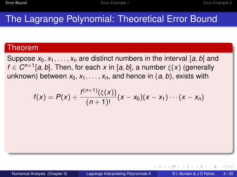
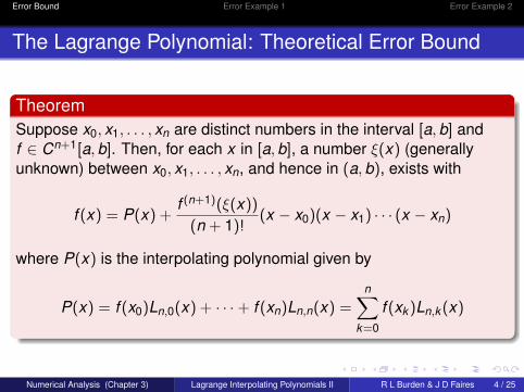
Suppose x0, x1, . . . , xn are distinct numbers in the interval [a, b] andf ∈ Cn+1[a, b]. Then, for each x in [a, b], a number ξ(x) (generallyunknown) between x0, x1, . . . , xn, and hence in (a, b), exists with
f (x) = P(x) +f (n+1)(ξ(x))
(n + 1)!(x − x0)(x − x1) · · · (x − xn)
where P(x) is the interpolating polynomial given by
P(x) = f (x0)Ln,0(x) + · · ·+ f (xn)Ln,n(x) =n∑
k=0
f (xk )Ln,k (x)
Numerical Analysis (Chapter 3) Lagrange Interpolating Polynomials II R L Burden & J D Faires 4 / 25
Error Bound Error Example 1 Error Example 2
The Lagrange Polynomial: Theoretical Error Bound
TheoremSuppose x0, x1, . . . , xn are distinct numbers in the interval [a, b] andf ∈ Cn+1[a, b].
Then, for each x in [a, b], a number ξ(x) (generallyunknown) between x0, x1, . . . , xn, and hence in (a, b), exists with
f (x) = P(x) +f (n+1)(ξ(x))
(n + 1)!(x − x0)(x − x1) · · · (x − xn)
where P(x) is the interpolating polynomial given by
P(x) = f (x0)Ln,0(x) + · · ·+ f (xn)Ln,n(x) =n∑
k=0
f (xk )Ln,k (x)
Numerical Analysis (Chapter 3) Lagrange Interpolating Polynomials II R L Burden & J D Faires 4 / 25
Error Bound Error Example 1 Error Example 2
The Lagrange Polynomial: Theoretical Error Bound
TheoremSuppose x0, x1, . . . , xn are distinct numbers in the interval [a, b] andf ∈ Cn+1[a, b]. Then, for each x in [a, b], a number ξ(x) (generallyunknown) between x0, x1, . . . , xn, and hence in (a, b), exists with
f (x) = P(x) +f (n+1)(ξ(x))
(n + 1)!(x − x0)(x − x1) · · · (x − xn)
where P(x) is the interpolating polynomial given by
P(x) = f (x0)Ln,0(x) + · · ·+ f (xn)Ln,n(x) =n∑
k=0
f (xk )Ln,k (x)
Numerical Analysis (Chapter 3) Lagrange Interpolating Polynomials II R L Burden & J D Faires 4 / 25
Error Bound Error Example 1 Error Example 2
The Lagrange Polynomial: Theoretical Error Bound
Error Bound: Proof (1/6)
Note first that if x = xk , for any k = 0, 1, . . . , n, then f (xk ) = P(xk ), andchoosing ξ(xk ) arbitrarily in (a, b) yields the result:
f (x) = P(x) +f (n+1)(ξ(x))
(n + 1)!(x − x0)(x − x1) · · · (x − xn)
If x 6= xk , for all k = 0, 1, . . . , n, define the function g for t in [a, b] by
g(t) = f (t)− P(t)− [f (x)− P(x)](t − x0)(t − x1) · · · (t − xn)
(x − x0)(x − x1) · · · (x − xn)
= f (t)− P(t)− [f (x)− P(x)]n∏
i=0
(t − xi)
(x − xi)
Numerical Analysis (Chapter 3) Lagrange Interpolating Polynomials II R L Burden & J D Faires 5 / 25
Error Bound Error Example 1 Error Example 2
The Lagrange Polynomial: Theoretical Error Bound
Error Bound: Proof (1/6)Note first that if x = xk , for any k = 0, 1, . . . , n, then f (xk ) = P(xk ), andchoosing ξ(xk ) arbitrarily in (a, b) yields the result:
f (x) = P(x) +f (n+1)(ξ(x))
(n + 1)!(x − x0)(x − x1) · · · (x − xn)
If x 6= xk , for all k = 0, 1, . . . , n, define the function g for t in [a, b] by
g(t) = f (t)− P(t)− [f (x)− P(x)](t − x0)(t − x1) · · · (t − xn)
(x − x0)(x − x1) · · · (x − xn)
= f (t)− P(t)− [f (x)− P(x)]n∏
i=0
(t − xi)
(x − xi)
Numerical Analysis (Chapter 3) Lagrange Interpolating Polynomials II R L Burden & J D Faires 5 / 25
Error Bound Error Example 1 Error Example 2
The Lagrange Polynomial: Theoretical Error Bound
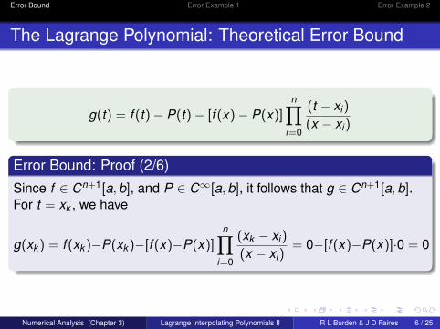
g(t) = f (t)− P(t)− [f (x)− P(x)]n∏
i=0
(t − xi)
(x − xi)
Error Bound: Proof (2/6)
Since f ∈ Cn+1[a, b], and P ∈ C∞[a, b], it follows that g ∈ Cn+1[a, b].For t = xk , we have
g(xk ) = f (xk )−P(xk )−[f (x)−P(x)]n∏
i=0
(xk − xi)
(x − xi)= 0−[f (x)−P(x)]·0 = 0
Numerical Analysis (Chapter 3) Lagrange Interpolating Polynomials II R L Burden & J D Faires 6 / 25
Error Bound Error Example 1 Error Example 2
The Lagrange Polynomial: Theoretical Error Bound
g(t) = f (t)− P(t)− [f (x)− P(x)]n∏
i=0
(t − xi)
(x − xi)
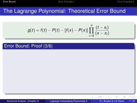
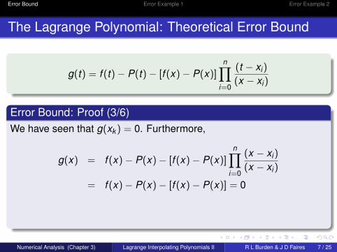
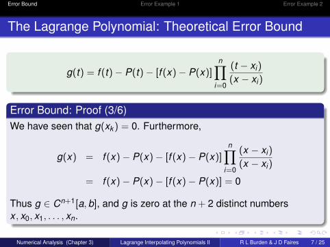
Error Bound: Proof (3/6)
We have seen that g(xk ) = 0. Furthermore,
g(x) = f (x)− P(x)− [f (x)− P(x)]n∏
i=0
(x − xi)
(x − xi)
= f (x)− P(x)− [f (x)− P(x)] = 0
Thus g ∈ Cn+1[a, b], and g is zero at the n + 2 distinct numbersx , x0, x1, . . . , xn.
Numerical Analysis (Chapter 3) Lagrange Interpolating Polynomials II R L Burden & J D Faires 7 / 25
Error Bound Error Example 1 Error Example 2
The Lagrange Polynomial: Theoretical Error Bound
g(t) = f (t)− P(t)− [f (x)− P(x)]n∏
i=0
(t − xi)
(x − xi)
Error Bound: Proof (3/6)We have seen that g(xk ) = 0. Furthermore,
g(x) = f (x)− P(x)− [f (x)− P(x)]n∏
i=0
(x − xi)
(x − xi)
= f (x)− P(x)− [f (x)− P(x)] = 0
Thus g ∈ Cn+1[a, b], and g is zero at the n + 2 distinct numbersx , x0, x1, . . . , xn.
Numerical Analysis (Chapter 3) Lagrange Interpolating Polynomials II R L Burden & J D Faires 7 / 25
Error Bound Error Example 1 Error Example 2
The Lagrange Polynomial: Theoretical Error Bound
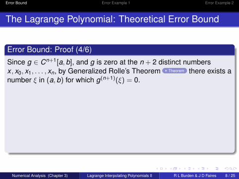
Error Bound: Proof (4/6)
Since g ∈ Cn+1[a, b], and g is zero at the n + 2 distinct numbersx , x0, x1, . . . , xn, by Generalized Rolle’s Theorem Theorem there exists anumber ξ in (a, b) for which g(n+1)(ξ) = 0.
So
0 = g(n+1)(ξ)
= f (n+1)(ξ)− P(n+1)(ξ)− [f (x)− P(x)]dn+1
dtn+1
[n∏
i=0
(t − xi)
(x − xi)
]t=ξ
However, P(x) is a polynomial of degree at most n, so the (n + 1)stderivative, P(n+1)(x), is identically zero.
Numerical Analysis (Chapter 3) Lagrange Interpolating Polynomials II R L Burden & J D Faires 8 / 25
Error Bound Error Example 1 Error Example 2
The Lagrange Polynomial: Theoretical Error Bound
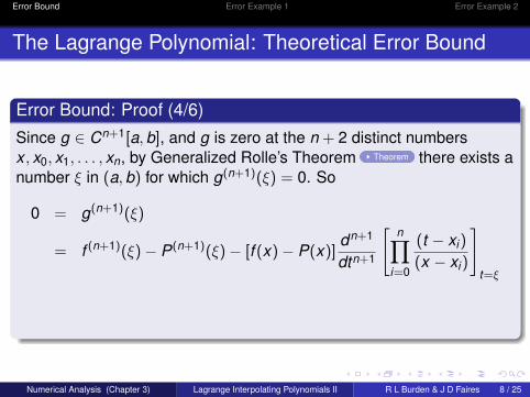
Error Bound: Proof (4/6)
Since g ∈ Cn+1[a, b], and g is zero at the n + 2 distinct numbersx , x0, x1, . . . , xn, by Generalized Rolle’s Theorem Theorem there exists anumber ξ in (a, b) for which g(n+1)(ξ) = 0. So
0 = g(n+1)(ξ)
= f (n+1)(ξ)− P(n+1)(ξ)− [f (x)− P(x)]dn+1
dtn+1
[n∏
i=0
(t − xi)
(x − xi)
]t=ξ
However, P(x) is a polynomial of degree at most n, so the (n + 1)stderivative, P(n+1)(x), is identically zero.
Numerical Analysis (Chapter 3) Lagrange Interpolating Polynomials II R L Burden & J D Faires 8 / 25
Error Bound Error Example 1 Error Example 2
The Lagrange Polynomial: Theoretical Error Bound
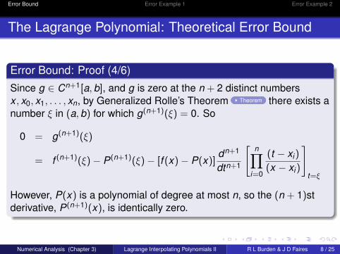
Error Bound: Proof (4/6)
Since g ∈ Cn+1[a, b], and g is zero at the n + 2 distinct numbersx , x0, x1, . . . , xn, by Generalized Rolle’s Theorem Theorem there exists anumber ξ in (a, b) for which g(n+1)(ξ) = 0. So
0 = g(n+1)(ξ)
= f (n+1)(ξ)− P(n+1)(ξ)− [f (x)− P(x)]dn+1
dtn+1
[n∏
i=0
(t − xi)
(x − xi)
]t=ξ
However, P(x) is a polynomial of degree at most n, so the (n + 1)stderivative, P(n+1)(x), is identically zero.
Numerical Analysis (Chapter 3) Lagrange Interpolating Polynomials II R L Burden & J D Faires 8 / 25
Error Bound Error Example 1 Error Example 2
The Lagrange Polynomial: Theoretical Error Bound
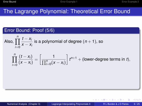
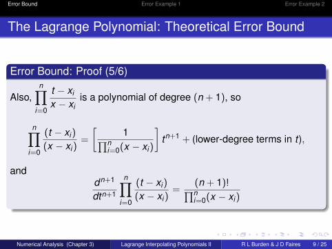
Error Bound: Proof (5/6)
Also,n∏
i=0
t − xi
x − xiis a polynomial of degree (n + 1), so
n∏i=0
(t − xi)
(x − xi)=
[1∏n
i=0(x − xi)
]tn+1 + (lower-degree terms in t),
anddn+1
dtn+1
n∏i=0
(t − xi)
(x − xi)=
(n + 1)!∏ni=0(x − xi)
Numerical Analysis (Chapter 3) Lagrange Interpolating Polynomials II R L Burden & J D Faires 9 / 25
Error Bound Error Example 1 Error Example 2
The Lagrange Polynomial: Theoretical Error Bound
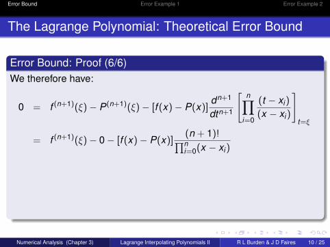
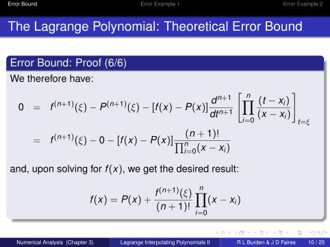
Error Bound: Proof (6/6)
We therefore have:
0 = f (n+1)(ξ)− P(n+1)(ξ)− [f (x)− P(x)]dn+1
dtn+1
[n∏
i=0
(t − xi)
(x − xi)
]t=ξ
= f (n+1)(ξ)− 0− [f (x)− P(x)](n + 1)!∏ni=0(x − xi)
and, upon solving for f (x), we get the desired result:
f (x) = P(x) +f (n+1)(ξ)
(n + 1)!
n∏i=0
(x − xi)
Numerical Analysis (Chapter 3) Lagrange Interpolating Polynomials II R L Burden & J D Faires 10 / 25
Error Bound Error Example 1 Error Example 2
The Lagrange Polynomial: Theoretical Error Bound
Error Bound: Proof (6/6)We therefore have:
0 = f (n+1)(ξ)− P(n+1)(ξ)− [f (x)− P(x)]dn+1
dtn+1
[n∏
i=0
(t − xi)
(x − xi)
]t=ξ
= f (n+1)(ξ)− 0− [f (x)− P(x)](n + 1)!∏ni=0(x − xi)
and, upon solving for f (x), we get the desired result:
f (x) = P(x) +f (n+1)(ξ)
(n + 1)!
n∏i=0
(x − xi)
Numerical Analysis (Chapter 3) Lagrange Interpolating Polynomials II R L Burden & J D Faires 10 / 25
Error Bound Error Example 1 Error Example 2
Outline
1 Interpolating Polynomial Error Bound
2 Example: 2nd Lagrange Interpolating Polynomial Error Bound
3 Example: Interpolating Polynomial Error for Tabulated Data
Numerical Analysis (Chapter 3) Lagrange Interpolating Polynomials II R L Burden & J D Faires 11 / 25
Lagrange Interpolating Polynomial Error Bound
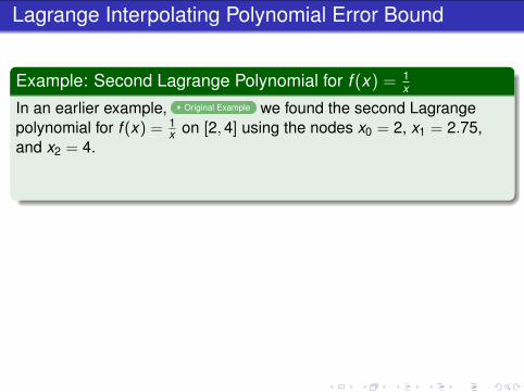
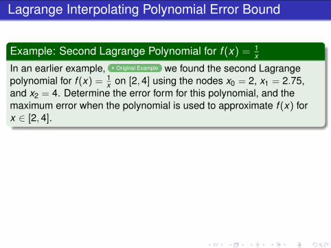
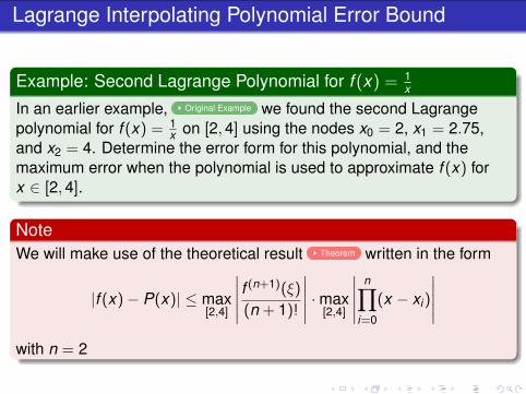
Example: Second Lagrange Polynomial for f (x) = 1x
In an earlier example, Original Example we found the second Lagrangepolynomial for f (x) = 1
x on [2, 4] using the nodes x0 = 2, x1 = 2.75,and x2 = 4.
Determine the error form for this polynomial, and themaximum error when the polynomial is used to approximate f (x) forx ∈ [2, 4].
NoteWe will make use of the theoretical result Theorem written in the form
|f (x)− P(x)| ≤ max[2,4]
∣∣∣∣∣ f (n+1)(ξ)
(n + 1)!
∣∣∣∣∣ ·max[2,4]
∣∣∣∣∣n∏
i=0
(x − xi)
∣∣∣∣∣with n = 2
Lagrange Interpolating Polynomial Error Bound
Example: Second Lagrange Polynomial for f (x) = 1x
In an earlier example, Original Example we found the second Lagrangepolynomial for f (x) = 1
x on [2, 4] using the nodes x0 = 2, x1 = 2.75,and x2 = 4. Determine the error form for this polynomial, and themaximum error when the polynomial is used to approximate f (x) forx ∈ [2, 4].
NoteWe will make use of the theoretical result Theorem written in the form
|f (x)− P(x)| ≤ max[2,4]
∣∣∣∣∣ f (n+1)(ξ)
(n + 1)!
∣∣∣∣∣ ·max[2,4]
∣∣∣∣∣n∏
i=0
(x − xi)
∣∣∣∣∣with n = 2
Error Bound Error Example 1 Error Example 2
The Lagrange Polynomial: 2nd Degree Error Bound
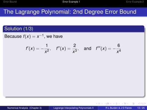
Solution (1/3)
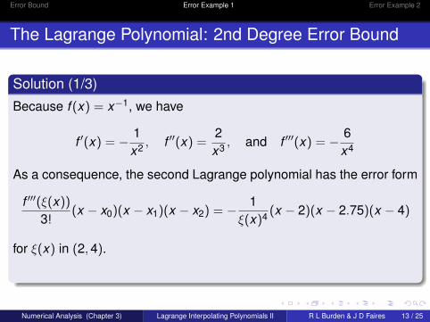
Because f (x) = x−1, we have
f ′(x) = − 1x2 , f ′′(x) =
2x3 , and f ′′′(x) = − 6
x4
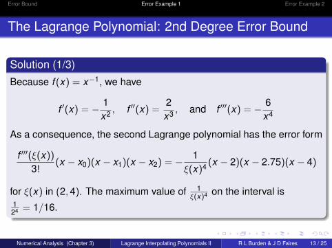
As a consequence, the second Lagrange polynomial has the error form
f ′′′(ξ(x))
3!(x − x0)(x − x1)(x − x2) = − 1
ξ(x)4 (x − 2)(x − 2.75)(x − 4)
for ξ(x) in (2, 4). The maximum value of 1ξ(x)4 on the interval is
124 = 1/16.
Numerical Analysis (Chapter 3) Lagrange Interpolating Polynomials II R L Burden & J D Faires 13 / 25
Error Bound Error Example 1 Error Example 2
The Lagrange Polynomial: 2nd Degree Error Bound
Solution (1/3)
Because f (x) = x−1, we have
f ′(x) = − 1x2 , f ′′(x) =
2x3 , and f ′′′(x) = − 6
x4
As a consequence, the second Lagrange polynomial has the error form
f ′′′(ξ(x))
3!(x − x0)(x − x1)(x − x2) = − 1
ξ(x)4 (x − 2)(x − 2.75)(x − 4)
for ξ(x) in (2, 4).
The maximum value of 1ξ(x)4 on the interval is
124 = 1/16.
Numerical Analysis (Chapter 3) Lagrange Interpolating Polynomials II R L Burden & J D Faires 13 / 25
Error Bound Error Example 1 Error Example 2
The Lagrange Polynomial: 2nd Degree Error Bound
Solution (1/3)
Because f (x) = x−1, we have
f ′(x) = − 1x2 , f ′′(x) =
2x3 , and f ′′′(x) = − 6
x4
As a consequence, the second Lagrange polynomial has the error form
f ′′′(ξ(x))
3!(x − x0)(x − x1)(x − x2) = − 1
ξ(x)4 (x − 2)(x − 2.75)(x − 4)
for ξ(x) in (2, 4). The maximum value of 1ξ(x)4 on the interval is
124 = 1/16.
Numerical Analysis (Chapter 3) Lagrange Interpolating Polynomials II R L Burden & J D Faires 13 / 25
Error Bound Error Example 1 Error Example 2
The Lagrange Polynomial: 2nd Degree Error Bound
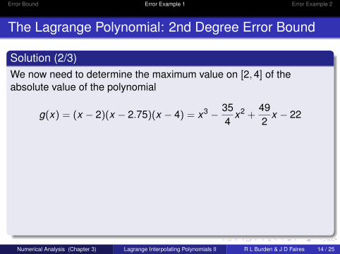
Solution (2/3)We now need to determine the maximum value on [2, 4] of theabsolute value of the polynomial
g(x) = (x − 2)(x − 2.75)(x − 4) = x3 − 354
x2 +492
x − 22
Because
g′(x) = 3x2 − 352
x +492
=12(3x − 7)(2x − 7),
the critical points occur at
x =73
with g(
73
)=
25108
and x =72
with g(
72
)= − 9
16
Numerical Analysis (Chapter 3) Lagrange Interpolating Polynomials II R L Burden & J D Faires 14 / 25
Error Bound Error Example 1 Error Example 2
The Lagrange Polynomial: 2nd Degree Error Bound
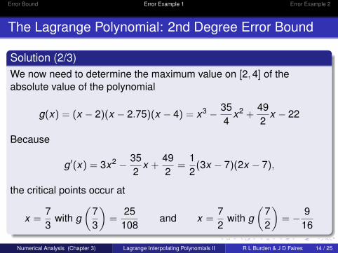
Solution (2/3)We now need to determine the maximum value on [2, 4] of theabsolute value of the polynomial
g(x) = (x − 2)(x − 2.75)(x − 4) = x3 − 354
x2 +492
x − 22
Because
g′(x) = 3x2 − 352
x +492
=12(3x − 7)(2x − 7),
the critical points occur at
x =73
with g(
73
)=
25108
and x =72
with g(
72
)= − 9
16
Numerical Analysis (Chapter 3) Lagrange Interpolating Polynomials II R L Burden & J D Faires 14 / 25
Error Bound Error Example 1 Error Example 2
The Lagrange Polynomial: 2nd Degree Error Bound
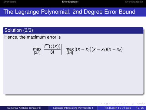
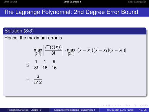
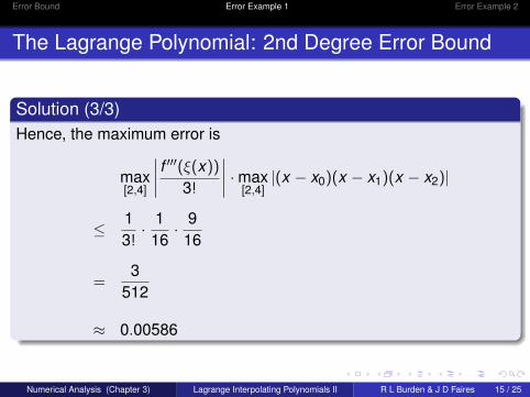
Solution (3/3)Hence, the maximum error is
max[2,4]
∣∣∣∣ f ′′′(ξ(x))
3!
∣∣∣∣ ·max[2,4]
|(x − x0)(x − x1)(x − x2)|
≤ 13!· 1
16· 9
16
=3
512
≈ 0.00586
Numerical Analysis (Chapter 3) Lagrange Interpolating Polynomials II R L Burden & J D Faires 15 / 25
Error Bound Error Example 1 Error Example 2
The Lagrange Polynomial: 2nd Degree Error Bound
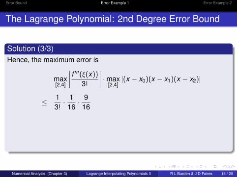
Solution (3/3)Hence, the maximum error is
max[2,4]
∣∣∣∣ f ′′′(ξ(x))
3!
∣∣∣∣ ·max[2,4]
|(x − x0)(x − x1)(x − x2)|
≤ 13!· 1
16· 9
16
=3
512
≈ 0.00586
Numerical Analysis (Chapter 3) Lagrange Interpolating Polynomials II R L Burden & J D Faires 15 / 25
Error Bound Error Example 1 Error Example 2
Outline
1 Interpolating Polynomial Error Bound
2 Example: 2nd Lagrange Interpolating Polynomial Error Bound
3 Example: Interpolating Polynomial Error for Tabulated Data
Numerical Analysis (Chapter 3) Lagrange Interpolating Polynomials II R L Burden & J D Faires 16 / 25
Use of the Interpolating Polynomial Error Bound
Example: Tabulated Data
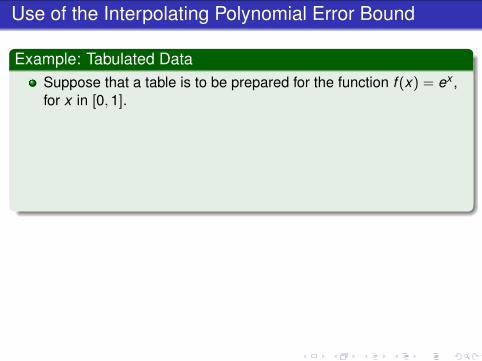
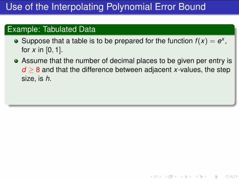
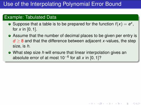
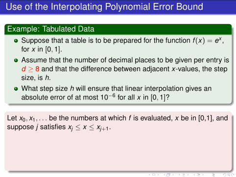
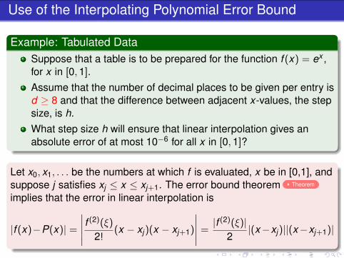
Suppose that a table is to be prepared for the function f (x) = ex ,for x in [0, 1].Assume that the number of decimal places to be given per entry isd ≥ 8 and that the difference between adjacent x-values, the stepsize, is h.What step size h will ensure that linear interpolation gives anabsolute error of at most 10−6 for all x in [0, 1]?
Let x0, x1, . . . be the numbers at which f is evaluated, x be in [0,1], andsuppose j satisfies xj ≤ x ≤ xj+1. The error bound theorem Theorem
implies that the error in linear interpolation is
|f (x)−P(x)| =
∣∣∣∣∣ f (2)(ξ)
2!(x − xj)(x − xj+1)
∣∣∣∣∣ =|f (2)(ξ)|
2|(x−xj)||(x−xj+1)|
Use of the Interpolating Polynomial Error Bound
Example: Tabulated DataSuppose that a table is to be prepared for the function f (x) = ex ,for x in [0, 1].
Assume that the number of decimal places to be given per entry isd ≥ 8 and that the difference between adjacent x-values, the stepsize, is h.What step size h will ensure that linear interpolation gives anabsolute error of at most 10−6 for all x in [0, 1]?
Let x0, x1, . . . be the numbers at which f is evaluated, x be in [0,1], andsuppose j satisfies xj ≤ x ≤ xj+1. The error bound theorem Theorem
implies that the error in linear interpolation is
|f (x)−P(x)| =
∣∣∣∣∣ f (2)(ξ)
2!(x − xj)(x − xj+1)
∣∣∣∣∣ =|f (2)(ξ)|
2|(x−xj)||(x−xj+1)|
Use of the Interpolating Polynomial Error Bound
Example: Tabulated DataSuppose that a table is to be prepared for the function f (x) = ex ,for x in [0, 1].Assume that the number of decimal places to be given per entry isd ≥ 8 and that the difference between adjacent x-values, the stepsize, is h.
What step size h will ensure that linear interpolation gives anabsolute error of at most 10−6 for all x in [0, 1]?
Let x0, x1, . . . be the numbers at which f is evaluated, x be in [0,1], andsuppose j satisfies xj ≤ x ≤ xj+1. The error bound theorem Theorem
implies that the error in linear interpolation is
|f (x)−P(x)| =
∣∣∣∣∣ f (2)(ξ)
2!(x − xj)(x − xj+1)
∣∣∣∣∣ =|f (2)(ξ)|
2|(x−xj)||(x−xj+1)|
Use of the Interpolating Polynomial Error Bound
Example: Tabulated DataSuppose that a table is to be prepared for the function f (x) = ex ,for x in [0, 1].Assume that the number of decimal places to be given per entry isd ≥ 8 and that the difference between adjacent x-values, the stepsize, is h.What step size h will ensure that linear interpolation gives anabsolute error of at most 10−6 for all x in [0, 1]?
Let x0, x1, . . . be the numbers at which f is evaluated, x be in [0,1], andsuppose j satisfies xj ≤ x ≤ xj+1.
The error bound theorem Theorem
implies that the error in linear interpolation is
|f (x)−P(x)| =
∣∣∣∣∣ f (2)(ξ)
2!(x − xj)(x − xj+1)
∣∣∣∣∣ =|f (2)(ξ)|
2|(x−xj)||(x−xj+1)|
Use of the Interpolating Polynomial Error Bound
Example: Tabulated DataSuppose that a table is to be prepared for the function f (x) = ex ,for x in [0, 1].Assume that the number of decimal places to be given per entry isd ≥ 8 and that the difference between adjacent x-values, the stepsize, is h.What step size h will ensure that linear interpolation gives anabsolute error of at most 10−6 for all x in [0, 1]?
Let x0, x1, . . . be the numbers at which f is evaluated, x be in [0,1], andsuppose j satisfies xj ≤ x ≤ xj+1. The error bound theorem Theorem
implies that the error in linear interpolation is
|f (x)−P(x)| =
∣∣∣∣∣ f (2)(ξ)
2!(x − xj)(x − xj+1)
∣∣∣∣∣ =|f (2)(ξ)|
2|(x−xj)||(x−xj+1)|
Error Bound Error Example 1 Error Example 2
Use of the Interpolating Polynomial Error Bound
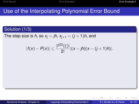
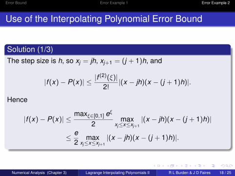
Solution (1/3)The step size is h, so xj = jh, xj+1 = (j + 1)h, and
|f (x)− P(x)| ≤ |f (2)(ξ)|2!
|(x − jh)(x − (j + 1)h)|.
Hence
|f (x)− P(x)| ≤maxξ∈[0,1] eξ
2max
xj≤x≤xj+1|(x − jh)(x − (j + 1)h)|
≤ e2
maxxj≤x≤xj+1
|(x − jh)(x − (j + 1)h)|.
Numerical Analysis (Chapter 3) Lagrange Interpolating Polynomials II R L Burden & J D Faires 18 / 25
Error Bound Error Example 1 Error Example 2
Use of the Interpolating Polynomial Error Bound
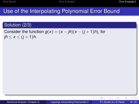
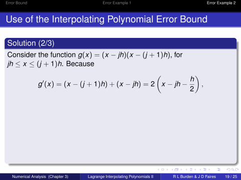
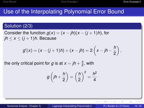
Solution (2/3)Consider the function g(x) = (x − jh)(x − (j + 1)h), forjh ≤ x ≤ (j + 1)h.
Because
g′(x) = (x − (j + 1)h) + (x − jh) = 2(
x − jh − h2
),
the only critical point for g is at x = jh + h2 , with
g(
jh +h2
)=
(h2
)2
=h2
4
Since g(jh) = 0 and g((j + 1)h) = 0, the maximum value of |g′(x)| in[jh, (j + 1)h] must occur at the critical point.
Numerical Analysis (Chapter 3) Lagrange Interpolating Polynomials II R L Burden & J D Faires 19 / 25
Error Bound Error Example 1 Error Example 2
Use of the Interpolating Polynomial Error Bound
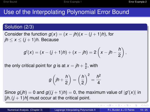
Solution (2/3)Consider the function g(x) = (x − jh)(x − (j + 1)h), forjh ≤ x ≤ (j + 1)h. Because
g′(x) = (x − (j + 1)h) + (x − jh) = 2(
x − jh − h2
),
the only critical point for g is at x = jh + h2 , with
g(
jh +h2
)=
(h2
)2
=h2
4
Since g(jh) = 0 and g((j + 1)h) = 0, the maximum value of |g′(x)| in[jh, (j + 1)h] must occur at the critical point.
Numerical Analysis (Chapter 3) Lagrange Interpolating Polynomials II R L Burden & J D Faires 19 / 25
Error Bound Error Example 1 Error Example 2
Use of the Interpolating Polynomial Error Bound
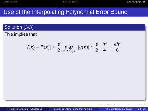
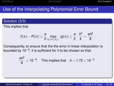
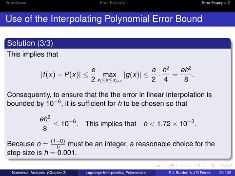
Solution (3/3)This implies that
|f (x)− P(x)| ≤ e2
maxxj≤x≤xj+1
|g(x)| ≤ e2· h2
4=
eh2
8.
Consequently, to ensure that the the error in linear interpolation isbounded by 10−6, it is sufficient for h to be chosen so that
eh2
8≤ 10−6. This implies that h < 1.72× 10⁻³.
Because n = (1−0)h must be an integer, a reasonable choice for the
step size is h = 0.001.
Numerical Analysis (Chapter 3) Lagrange Interpolating Polynomials II R L Burden & J D Faires 20 / 25
Error Bound Error Example 1 Error Example 2
Use of the Interpolating Polynomial Error Bound
Solution (3/3)This implies that
|f (x)− P(x)| ≤ e2
maxxj≤x≤xj+1
|g(x)| ≤ e2· h2
4=
eh2
8.
Consequently, to ensure that the the error in linear interpolation isbounded by 10−6, it is sufficient for h to be chosen so that
eh2
8≤ 10−6. This implies that h < 1.72× 10⁻³.
Because n = (1−0)h must be an integer, a reasonable choice for the
step size is h = 0.001.
Numerical Analysis (Chapter 3) Lagrange Interpolating Polynomials II R L Burden & J D Faires 20 / 25

Questions?

Reference Material
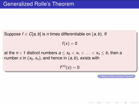
Generalized Rolle’s Theorem
Suppose f ∈ C[a, b] is n times differentiable on (a, b). If
f (x) = 0
at the n + 1 distinct numbers a ≤ x0 < x1 < . . . < xn ≤ b, then anumber c in (x0, xn), and hence in (a, b), exists with
f (n)(c) = 0
Return to Error Bound Theorem
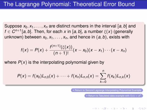
The Lagrange Polynomial: Theoretical Error Bound
Suppose x0, x1, . . . , xn are distinct numbers in the interval [a, b] andf ∈ Cn+1[a, b]. Then, for each x in [a, b], a number ξ(x) (generallyunknown) between x0, x1, . . . , xn, and hence in (a, b), exists with
f (x) = P(x) +f (n+1)(ξ(x))
(n + 1)!(x − x0)(x − x1) · · · (x − xn)
where P(x) is the interpolating polynomial given by
P(x) = f (x0)Ln,0(x) + · · ·+ f (xn)Ln,n(x) =n∑
k=0
f (xk )Ln,k (x)
Return to Second Lagrange Interpolating Polynomial Example
Return to Tabulated data example with f (x) = ex
The Lagrange Polynomial: 2nd Degree Polynomial
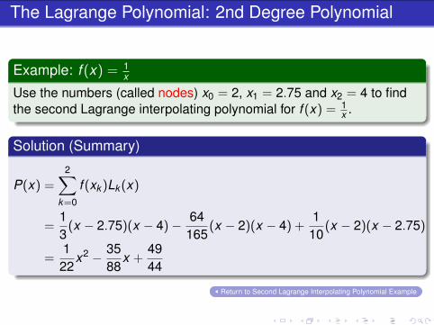
Example: f (x) = 1x
Use the numbers (called nodes) x0 = 2, x1 = 2.75 and x2 = 4 to findthe second Lagrange interpolating polynomial for f (x) = 1
x .
Solution (Summary)
P(x) =2∑
k=0
f (xk )Lk (x)
=13(x − 2.75)(x − 4)− 64
165(x − 2)(x − 4) +
110
(x − 2)(x − 2.75)
=122
x2 − 3588
x +4944
Return to Second Lagrange Interpolating Polynomial Example
![Interpolation & Polynomial Approximation [0.125in]3.625in0.02in …mamu/courses/231/Slides/CH03_3A.pdf · 2012-08-02 · Interpolation & Polynomial Approximation Divided Differences:](https://img.pdfslide.net/doc/110x75/5f5234d5ff877a36963dc704/interpolation-polynomial-approximation-0125in3625in002in-mamucourses231slidesch033apdf.jpg)
![Interpolation & Polynomial Approximation [0.125in]3.625in0 ... · IntroductionNotationNewton’s Polynomial Outline 1 Introduction to Divided Differences 2 The Divided Difference](https://img.pdfslide.net/doc/110x75/5f5234d7ff877a36963dc70c/interpolation-polynomial-approximation-0125in3625in0-introductionnotationnewtonas.jpg)


![Interpolation & Polynomial Approximation [0.125in]3.625in0](https://img.pdfslide.net/doc/110x75/61caec2c5334682d856ac40e/interpolation-amp-polynomial-approximation-0125in3625in0-.jpg)
