UNIVERSITA DEGLI STUDI DI PADOVADipartimento di Fisica e Astronomia ”G. Galilei”

Corso di Laurea magistrale in FisicaPercorso teorico e modellistico

Matteo Abbate

Interpretation of chromosome conformationcapture data in terms of graphs.

Tesi finale di Laurea magistrale

SUPERVISOR ERASMUS:Prof. Dieter W. Heermann,Institute for Theoretical Physics, Ruprecht-Karls Universitaet HeidelbergINTERNAL SUPERVISOR:Prof. Flavio Seno

Academic Year 2015/2016

Ai miei genitori.

1

Contents

1 Introduction 5

2 Theory 82.1 Chromosome Conformation Capture . . . . . . . . . . . . . . 82.2 Spectral Graph Theory . . . . . . . . . . . . . . . . . . . . . . 122.3 Distances in graph theory . . . . . . . . . . . . . . . . . . . . 182.4 The embedding problem . . . . . . . . . . . . . . . . . . . . . 292.5 Embedding of a graph . . . . . . . . . . . . . . . . . . . . . . 36

3 Results 383.1 Introduction . . . . . . . . . . . . . . . . . . . . . . . . . . . . 383.2 Test of the Multidimensional scaling . . . . . . . . . . . . . . 383.3 Hi-C simulations data . . . . . . . . . . . . . . . . . . . . . . 413.4 Real data . . . . . . . . . . . . . . . . . . . . . . . . . . . . . 51

4 Other applications 564.1 Introduction . . . . . . . . . . . . . . . . . . . . . . . . . . . . 564.2 Bayesian method . . . . . . . . . . . . . . . . . . . . . . . . . 584.3 New frequency method . . . . . . . . . . . . . . . . . . . . . . 59

5 Conclusions 71

6 Appendix A 74

7 Appendix B 76

Acknowledgments 90

4

1 Introduction

The cell is the fundamental unit that characterizes any living being. Fromthe simplest organisms, the prokaryotes, which have only one cell, throughthe most complex as the human organisms that contain around 100 thou-sands billions cells in their bodies, the concept of life of the cell is alwaysstrictly connected to its capacity to duplicate itself.Duplicating consists of generating another cell that is able to build by itselfthe same molecules that allow the mother cell to lead all its biochemicalprocesses. All the information necessary to generate these molecules are con-tained in the genome of a cell. It consists of chains of molecules called DNA.During the duplication process, the genome is copied and transferred to thedaughter cell. According to the amount of information that the genome cancarry, its chains can achieve huge lengths and generally they must be com-pacted by nearly three orders of magnitude to fit within the limited volumeof a cell. Hence, they are organized in compacted structures called chromo-somes.Therefore, understanding how chromosomes duplicate and how they are ex-pressed, i.e. how they generate proteins, is fundamental in order to discoverhow life works. Furthermore, investigating gene expression can provide in-struments that are useful to understanding diseases due to genetic mutations.Many studies confirmed that local structural properties of the chromosomescan influence gene expression, DNA replication and repairing [1] [57] [15] [13].Understanding how chromosomes fold can provide insight into the relation-ship between the chromatine structure and its functional activity.Despite its importance, discovering higher order structural features is stillcomplicated due to technical limitations. Some traditional high resolutionmeasurements like electron microscopy or fluorescence are not easily applica-ble or don’t provide information about the entire genome. Other techniquessuch as light microscopy don’t achieve sufficient resolution instead.Recently a new methodology has been proposed [17]. It provides high-resolution topological information for an entire genome. In fact, the Captur-ing Chromosome Conformation (or 3C) technique consists of counting howoften different loci of a genome interact with each other. The resolution ofthe experiment has been recently increased and the most recent measure-ments at higher resolution are referred to as Hi-C method [37].Hence, this technique yields a set of relative frequencies of contact betweendifferent parts of the same genome. These data, usually presented in matrix

5

form, can be used to analyze the overall spatial organization of the chromo-somes. In particular, it is reasonable to assume that the contact frequencybetween two loci is somehow related to their distance: the bigger the fre-quency, the smaller the expected distance.The goal of this work is to obtain a consistent method to reconstruct thethree dimensional structure of the chromosome by means of the Hi-C data.In particular, this thesis is inspired by a previous technique that interpretsthe Hi-C data in terms of graph theory. Graph theory is the theory of math-ematical structures called graphs which consist of a set of vertexes connectedby edges. Its applications are widespread: from physics to psychology, fromsociometry to linguistic. In this case, we will apply it to a biological problem.We will consider each locus of the genome as a vertex of the graph and eachcontact frequency between two loci as a weight to associate to the edge con-necting them.The problem of drawing a graph in a 3 dimensional space is also known asthe so-called embedding problem. A solution of this problem is the Multidi-mensional scaling method (MDS) [59] [54]. Given a set of distances betweenthe vertexes of a graph, this method returns an Euclidean set of coordinates.Hence, we will propose different ways to define distances between the ver-texes of a graph and we will investigate which are the conditions that it mustsatisfy in order to solve the embedding problem. In particular, we will stressthe use of a matrix called Laplacian matrix of the graph, demonstrating thatits spectrum and its eigenvectors have some interesting properties. We willshow that a distance called effective resistance yields to the most consistentreconstruction.Some simulations of Hi-C data will be performed in order to verify the the-oretical statements, focusing on polymers with a linear, circular or rosetteconformation.The thesis work is organized as follows: in the first chapter we will presenta theoretical approach to the problem remarking some knowledge of graphtheory and proposing some definitions for distances. Then the embeddingproblem and the multidimensional scaling method are described both gen-erally and in the case of the previously defined distances. In the secondchapter some results are presented, showing the consistence of the MDS forsimulated polymers and applying it to a set of real Hi-C data. Finally, in thelast chapter we will propose some further applications of the MDS method. Inparticular, we will see how to combine Hi-C data with fluorescence measure-ments. The latter provide a set of directly measured distances between just

6

few loci. We will present two different methods, showing their advantagesand their limits.

7

2 Theory

2.1 Chromosome Conformation Capture

The biological unit of any living organism is the cell. It contains all themolecules that take part to the main biological processes, but, most impor-tantly, it is the smallest unit able to replicate independently. This is thebasic concept of life. In fact, the cell is able to divide itself in two parts,duplicating some particular molecules that contain all the biological infor-mation, i.e. that can then produce all the other useful biomolecules.The molecules that carries all these genetic instructions are the deoxidribonu-cleic acid (DNA). They consist of long chains with the shape of a double helix.They are polymers composed by repeating units called nucleotides. Thereare 4 different kinds of nucleotides and their particular sequence in the chaindecodes for the production of specific biomolecules.Since the DNA carries all the information necessary to the growth of the cell,it contains a huge amount of nucleotides. The length of a DNA sequence isusually measured in base pair (bp), that is a unit consisting of two couplednucleotides. Each filament contains several millions nucleotides and each cellmay contain many filaments of DNA. This means that the length of a DNAchain can be very high and it must be compacted nearly by three orders ofmagnitude to fit the limited volume of a cell. This is the reason why DNA isnot usually found on its own, but it is organized in packaged structures callednucleoids in the bacteria [45] and chromosomes in the eukaryotes, where theyare confined inside the nucleus of the cell. The importance of chromosomesand nucleoids is hence fundamental, because they are the instrument thatevery living being uses to transmit life.The number of chromosomes per cell is specific of the organism. The hu-man cell has got 46 chromosomes, the dog’s cell 78 and the prokaryotes’ cell,monocellular organisms, just one. The shape of the chromosomes is highlydynamic: it is different in each type of organism and changes even duringthe different phases of the life of the cell. For example, in the prokaryotesthe chromosome is circular, while in the human cell it can have an X shapeduring the metaphase of the cell. In this case the chromosome is said to beacrocentric.The structural properties and the spatial conformations of chromosomes havebeen linked with important chromosomal activities [57]. It has been proventhat even local high order structural features such as loops, axes, interchro-

8

mosomal connections have important roles in the genetic expressions, i.e. inthe way the DNA is decoded in order to produce biomolecules. For instance,the time of replication has been linked to the spatial disposition of differentregions of the chromosomes [1] [15] [13].

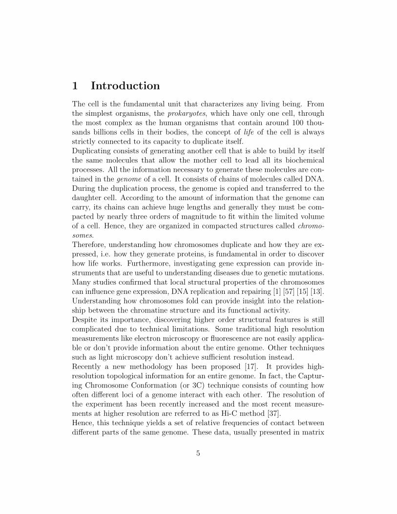
Despite its importance, the investigation of the chromosome spatial con-formation is limited by technical limitations. In fact, light microscopy doesn’treach a sufficient resolution and electron microscopy, which would allow tohave high resolution, is not easily applicable to study specific loci of thechromosome. The fluorescence technique consists in fusing some fluorescentprotein with the chromosome and permits the visualization of individual loci,but only few positions can be examined simultaneously. The FISH (Fluores-cence In Situ Hybridization) technique permits to visualize multiple loci, butit requires several treatments that may affect the chromosome conformation.A significant contribution to the exploration of the structure of the chro-mosomes has been given by Dekker at al. in 2002 [17]. They proposed amethodology called Capturing Chromosome Conformation (3C) to charac-terize some overall physical properties at high resolution.It consists in isolating the part of the cell where the chromosome are andsubject them to a process called formaldehyde fixation (Fig. 1). This pro-cess creates cross-links between different parts of the DNA through proteins.A cross-link determines a contact between different segments of the DNA.Then each contact is counted and the relative frequency with which differentloci have become cross-linked is registered, by means of a reaction calledquantitative PCR (Polymerase chain reaction).

In principle, the 3C method required to choose a set of target loci andcount the cross links among them. A technique to obtain an unbiasedgenomewide analysis, i.e. through the entire DNA sequences, was proposedin 2009 [37]. Since it improved the resolution of the 3C measure, it has beencalled Hi-C. In the following years, the resolution has been further increased[19] [44] and today we may have a precision of 1 kilobase for the humangenome.The results of the Hi-C measure are usually represented in a matrix form. IfN is the number of loci analyzed, an N ×N matrix W is used. The entrieswij represent the relative frequency of contacts between the loci i and j. Thiscan be visualized in an heat map (Fig. 2 and 3). The use of these topologicalinformation has permitted to individuate some regions of the chromosomes

9

Figure 1: Capturing Chromosome Conformation process. [Adapted from: [17]]Schematic representation of the assay: first the cross-link is created using the formalde-hyde. Then, after the EcoRI molecule digestion and intramolecular ligation, the PCRmediates the detection of the ligation products, after reversal of the cross link.

that are closer in space through the analysis of particular patterns of thematrix.

Despite these results, an exact three dimensional chromosomes’ confor-mation has not been given yet. A possible use of these information to arisea 3D reconstruction of the structure has been proposed by Lesne et al. [35].In this case, the matrix W has been interpreted as the adjacency matrix ofa weighted graph. This interpretation may be extended and raised to otherapplications. Because of this, it will be investigated deeply in the next sec-tions, beginning from some remarks of the general graph theory.

10

Figure 2: Example of Hi-C output. [Adapted from: [37]] Hi-C produces a genomewidecontact matrix. The matrix shows the intrachromosomal interactions on chromosome 14.It is acocentric; the short arm is not shown. The dimension of each pixel is 1Mb locus.Intensity corresponds to the total number of reads (0 to 50).

Figure 3: Example of Hi-C output. [Adapted from: [34]] A normalized Hi-C contactmap of a bacterial chromosome is presented. The Caulobacter crescentus chromosome iscircular which can be noted in the off-diagonal intensity. It consists of multiple, largelyindipendent spatial domains likely comprised.

11

2.2 Spectral Graph Theory

A graph G = (V,E) is a set of points V called vertexes connected by linkscalled edges represented by E.The graph order is the number n of its vertexes. The graph size is the num-ber m of its edges. The vertex degree is the number of the edges departingfrom that vertex.A graph is undirected if the edges have not orientation and directed or di-graph if they have an orientation and may be represented by an arrow (Fig.4 a-b). A loop is an edge that connects a vertex with itself.A multiple graph is a graph in which two vertexes can be connected by twoor more edges. A simple graph is an undirected graph which does not containmultiple edges or loops. A path between two vertexes i and j is an orderedsequence of consecutive edges starting from i and ending in j.

The structure of a graph is usually represented by means of a matrixcalled adjacency matrix A whose entries aij are 0 if vertexes i,j are not con-nected and 1 otherwise. Obviously, the matrix of an undirected graph issymmetric. Let’s give now some additional definitions.A complete graph is a graph in which each pair of vertexes is connected byan edge (Fig. 4 c).A weighted graph is a graph in which each edge is equipped with a numbercalled weight. In this case the adjacency matrix entries wij correspond tothe weight of the ij edge and the vertex degree is defined as the sum of theweights of all its vertexes. The degree matrix K of a graph is a diagonalmatrix, whose diagonal consists of the degrees of the vertexes of the graph.A graph is connected if for each pair of vertexes at least one path existsbetween them. It is disconnected otherwise (Fig. 4 d). This means that itis always possible to reach a vertex from another one. A connected compo-nent of a graph is a subgraph in which two vertexes are always connectedby a path and which is not connected to any other vertex of the graph. Aconnected graph has got one connected component and a complete graph isalways connected.A tree is an acyclic connected undirected graph, i.e. a graph where any two

vertexes are connected by exactly one path. A forest is a disjoint union oftrees.

Let’s now consider a simple complete weighted graph. We will give an

12

Figure 4: Examples of graphs. a) Directed graph b) Undirected graph c) Completeundirected graph d) Connected graph that becomes disconnected when the thedashededge is removed.

important definition that is adaptable in the case of unweighted graphs sim-ply substituting each nonzero weight with 1.The Laplacian Matrix of a graph is defined as L = K − A:

L =

k1 −w12 ... −w1n

−w12 k2 ... −w2n

... ... ... ...−wn1 −wn2 ... kn

or for each component lij = δijkij − wij.This matrix is important because it allows us to unveil some topologicalproperties of the graph.The name “Laplacian” derives from the fact that the i-th row of the matrixgives the value of the discrete Laplacian operator on the vertex i in N di-mensions [5]. In fact, a Laplacian operator (for the sake of simplicity hererepresented in 3 dimensions and for an unweighted graph) applied to a func-tion φ(x, y, z) is defined as:

∇2φ(x, y, z) =∂2φ(x, y, z)

∂x+∂2φ(x, y, z)

∂y+∂2φ(x, y, z)

∂z

When the function is defined only for discrete values, the derivative is sub-stituted by the finite differences:

φ(x+ 1, y, z)− φ(x, y, z) = φ(x, y, z)− φ(x− 1, y, z)

Hence, the Laplacian becomes:

∇2φ(x, y, z) =∑α,β,γ

φ(α, β, γ)− kφ(x, y, z)

13

where α, β, γ indicate the coordinates of the neighbors to x, y, z. The rela-tionship between the Laplacian operator and the matrix is clear comparingthis result with any sum of the entries of a row of the Laplacian matrix (witha minus sign).As it will be clear later, the Laplacian matrix is also analogous to the Laplace-Beltrami operator on manifolds.

The study of the graph Laplacian eigenvalues is known as spectral graphtheory [12] [51]. It has been developed in the past decades in order to todeduce the principal properties and structure of a graph from its Laplacianspectrum, showing that there is an interesting analogy with spectral Rie-mann differential geometry.Furthermore, it has been proven that the Laplacian spectra is strictly influ-enced by topological factors, as clustering, symmetries and degree distribu-tion [39]. We define now the normalized Laplacian as

L = T−1/2LT−1/2

where T denotes the diagonal matrix with i-th entry∑

j wij.

We can view it as an operator in the space of the continuous functionsg : V (G)→ R which satisfies [12]

Lg(u) =1√ku

∑v,u∼v

(g(u)√ku− g(v)√

kv

)wuv

Since L is symmetric with non negative entries, its eigenvalues are all realand non-negative. By construction, the Laplacian matrix kernel has at leastdimension 1, i.e. it has a 0 eigenvalue whose corresponding eigenvector isthe constant eigenvector (with all entries equal). We can calculate the othereigenvalues in terms of the Rayleigh quotient of L [41]. Let g be an arbitraryfunction that assigns a value g(v) to each vertex v of the graph. Using thenotation 〈,〉 to indicate the standard inner product in Rn, the Rayleigh quo-tient of L is then

〈g,Lg〉〈g, g〉

=〈f, Lf〉

〈T 1/2f, T 1/2f〉=

∑u∼v wuv(f(u)− f(v))2∑

v(f(v))2kv

where g = T 1/2f and the∑

u∼v sums up all the pairs of adjacent vertexes.The minimum value of the Rayleigh quotient corresponds to the minimum

14

eigenvalue of L. It is easy to see it is 0, letting f be a trivial function thatassigns a constant value to each vertex. The first smallest eigenvalue after0 is the the smallest value of the Rayleigh quotient, when f is a functionorthogonal to the trivial one.In the non trivial case the functions f are usually called harmonic eigenfunc-tions of L. For their particular properties, these functions often find manyapplications, e.g. in video imaging. In fact, in order to solve PDE problems,they can be used as eigenfunctions for a mesh refinement process and theyrespect the symmetries of the surface of the grid [36].The above formulation for the non trivial eigenvalue corresponds in a naturalway to the eigenvalues of the Laplacian-Beltrami operator [3] that we willdefine now in the unweighted case. Considering a smooth m-dimensionalmanifold M embedded in Rk, the Riemann structure on the manifold is in-duced by the standard Riemann structure on Rk. Let now f be a mapf : M → R, then the Laplace-Beltrami operator is defined as L = ∇ · ∇f .For the Stokes theorem then:∫

M

‖∇f‖2 =

∫M

L(f)f

We see that L is positive semidefinite and the f that minimizes∫M‖∇f‖2

has to be an eigenfunction of L. We further notice then that the gradient∇f is a vector field on the manifold, such that for small δx:

|f(x+ δx)− f(x)| ≈ |〈∇f(x), δx〉| ≤ ‖∇f‖‖δx‖

The eigenvalues for the Laplace-Beltrami operator are thus:

λM = inf

∫M‖∇f‖2∫Mf 2

For a general k-th eigenvalue of the Laplacian matrix, we have

λk = inff⊥TPk−1

∑u∼v wuv(f(u)− f(v))2∑

v f(v)2kv

where Pk−1 denotes the subspace generated by the harmonic eigenfunctionscorresponding to the eigenvalues smaller than λk. Let’s now show the follow-ing [12]:

15

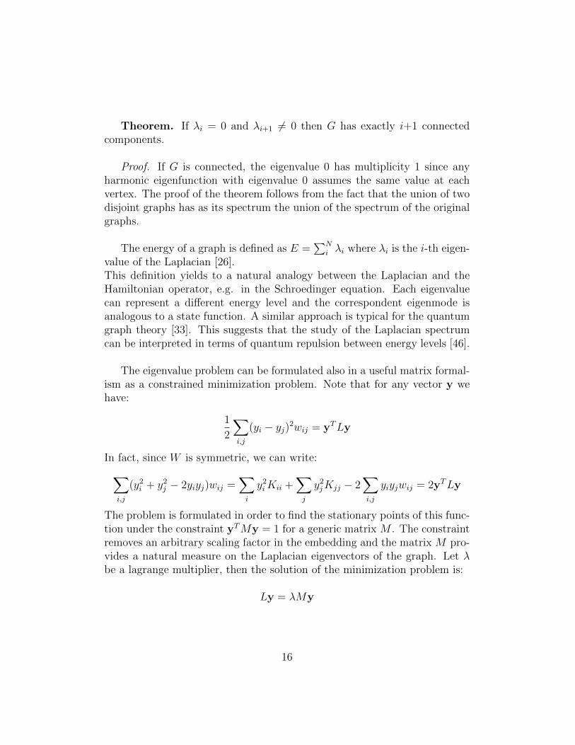
Theorem. If λi = 0 and λi+1 6= 0 then G has exactly i+1 connectedcomponents.

Proof. If G is connected, the eigenvalue 0 has multiplicity 1 since anyharmonic eigenfunction with eigenvalue 0 assumes the same value at eachvertex. The proof of the theorem follows from the fact that the union of twodisjoint graphs has as its spectrum the union of the spectrum of the originalgraphs.

The energy of a graph is defined as E =∑N

i λi where λi is the i-th eigen-value of the Laplacian [26].This definition yields to a natural analogy between the Laplacian and theHamiltonian operator, e.g. in the Schroedinger equation. Each eigenvaluecan represent a different energy level and the correspondent eigenmode isanalogous to a state function. A similar approach is typical for the quantumgraph theory [33]. This suggests that the study of the Laplacian spectrumcan be interpreted in terms of quantum repulsion between energy levels [46].

The eigenvalue problem can be formulated also in a useful matrix formal-ism as a constrained minimization problem. Note that for any vector y wehave:

1

2

∑i,j

(yi − yj)2wij = yTLy

In fact, since W is symmetric, we can write:∑i,j

(y2i + y2j − 2yiyj)wij =∑i

y2iKii +∑j

y2jKjj − 2∑i,j

yiyjwij = 2yTLy

The problem is formulated in order to find the stationary points of this func-tion under the constraint yTMy = 1 for a generic matrix M . The constraintremoves an arbitrary scaling factor in the embedding and the matrix M pro-vides a natural measure on the Laplacian eigenvectors of the graph. Let λbe a lagrange multiplier, then the solution of the minimization problem is:

Ly = λMy

16

Let’s now analyze what happens with different choices of the metric con-straint M :

• choosing M = 1 leads to Ly = λy with the constraint yTy = 1, henceit is equivalent to solve the eigenvalues problem for the Laplacian;

• choosing M as a general diagonal matrix whose eigenvectors are yleads to Ly = λλMy = λLy , hence the lagrange multiplier is equalto λ = λL

λM. In this particular example we can see how

√λM gives

naturally a metric to each eigenvector of the Laplacian. In fact, sinceLy = λLy, then we can simply solve the minimization problem as

λMyTLy = y′TLy′ =

1

2

∑i,j

(y′i − y′j)2wij

with y′ =√λMy ;

• for some reasons that will be clear later, let’s show a particular case inwhich M is a general matrix symilar to a diagonal matrix, i.e. such thatM = xTΛx = x′Tx′ where x′ = Λ1/2x with the condition xT1x = 1.Then (xy)TΛ(xy) = 1. Suppose now that for some particular eigenvec-tors y = x/

√λM holds, i.e. the eigenvectors of M and L are parallel.

In this case the constraint condition is always true and the minimiza-tion problems is solved by Ly = λ√

λMMx = λλMy = λLy i.e. again

λ = λL/λM .In the trivial case in which all the eigenvalues of M are equal to 1, weobtain the generalization of the previous case when M is symilar to theidentity matrix.

Let’s note that, according to the definition of energy of a graph given aboveand considering the case in which M = 1, we have:

E =∑i

λLi =∑i

yTi Lyi

Hence we can redefine the energy in one of the previous general cases as:

E =∑i

y′Ti Ly′i =

∑i

λMi λLi

17

That can be interpreted as an energy in which the eigenvalues λM give aweight to each energetic eigenvalue of the Laplacian, according to the chosenmetric.

The eigenvectors will represent the eigenmodes of the system. The firstone, corresponding to the mode of null energy, is the constant vector andrepresents the trivial equilibrium case in which all the points have the samecoordinates.

2.3 Distances in graph theory

We will now remark some basic concepts of general topology, beginning withthe definition of a distance, in order to apply it later in the graph theory.

Definition. A metric or distance on a set X is a function d : X ×X →[0,∞) such that satisfies the following conditions:

1. non negativity: d(x, y) ≥ 0 for any x,y and d(x, y) = 0 iff x = y;

2. symmetry: d(x, y) = d(y, x);

3. triangle inequality: d(x, z) ≤ d(x, y) + d(y, z) for any x,y,z ∈ X.

Definition. Given a vector space V a norm on V is a function ‖ · ‖ :V → R such that:

1. ‖av‖ = a‖v‖ for a ∈ R

2. ‖(v + w)‖ ≤ ‖v‖+ ‖w‖

3. ‖v‖ = 0 iff v is the zero vector.

It follows that ‖v‖ ≥ 0 for any v ∈ V .

Definition. Two norms are equivalent if α‖x‖1 < ‖x‖2 < β‖x‖1 forsome real numbers α, β ≥ 0.

Theorem. All norms are equivalent in a finite dimensional space.

18

It is possible to define a distance induced by a norm as d(x, y) = ‖(x−y)‖.

Definition. Given a set X a topology T is a subset of the partition setP(X) such that:

1. 0 ∈ T , X ∈ T

2. The union of elements of T still belongs to T

3. The intersection of a finite number of elements of T belongs to T

The elements of T are called open sets.

A metric can naturally induce a topology, simply defining an open set asthe set of all elements y such that d(x, y) < r where r is called radius of theopen set.

Definition. Two metrics d and D on X are equivalent if all open sub-sets of X are equal with respect of d and D. They are strongly equivalent ifαd < D < βd for some real numbers α, β > 0.

These definitions leads to an important theorem [40].

Theorem. In Rn all the metrics induced by a norm are equivalent, i.e.they induce the same topology.

This is generally not true if the distance is not induced by a norm. Wewill now introduce a general way to define a distance not induced by a normin a discrete space X, hence applicable in the graph space. This method isbased on the following definition of proximity matrix. Proximity measuresfor the vertexes of directed and undirected graphs arise in a wide range ofapplications, from cristallography to mathematical sociology (applied, for in-stance, to the social networks).

We will introduce it in the discrete case, since this case will be useful forour applications [10].

Definition. Let X be a discrete set of dimension n. A proximity (oraccessibility or connectedness) measure is a function p : X × X → [0,∞)

19

that can be represented by a n× n matrix P and that satisfies the followingconditions for any multigraph:

1. non negativity: pij ≥ 0 for any i, j = 1, . . . n;

2. symmetry: the matrix P is symmetric;

3. reversal property: if the graph is directed, the reversal of all its arcsresults in the transposition of the proximity matrix;

4. diagonal maximality: for any i, j = 1, . . . n such that i 6= j, pii > pijand pii > pji holds;

5. triangle inequality for proximities: for any i, j, k = 1, . . . n pij + pik −pjk ≤ pii holds. If then j = k and i 6= j the inequality is strict.

The definition of this matrix will be very useful because, as we will see, some-times it is easier to define a map that satisfies the above triangle inequality,rather than the distance one. Nevertheless, a simple theorem allows us toconstruct a metric through the use of a proximity measure.

Theorem. Consider the quantity dij = pii + pjj − pij − pji with i, j =1, . . . n. This defines a distance, i.e. it satisfies the axioms of a metric.

In fact, provided that p satisfies the conditions and the triangle inequalityof a proximity measure, then d satisfies the triangle inequality for a distance.

In the matrices formalism the distance matrix can be written as:

D = 1diagP T + diagP1T − 2P

We are now ready to give some definitions of distances for graphs, us-ing both traditional definitions or definition through the use of proximities.In particular we will focus on: shortest path distance, resistance distance,connectedness distances, Laplacian distance, natural proximity distance, en-tropy distance and potential proximity distance, Katz proximity distance.

Shortest path distance. Let’s define the length of an edge as the in-verse of its weight and the length of a path as the sum of lengths of all theedges belonging to that path. Considering all possible paths between two

20

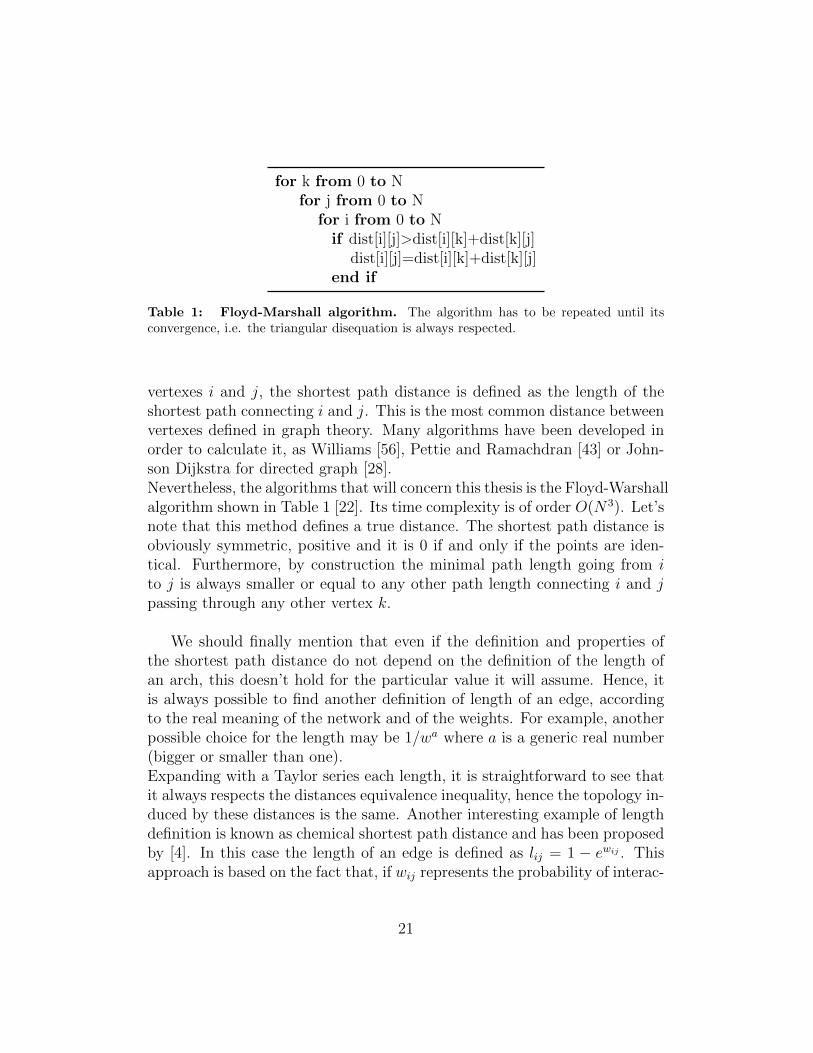
for k from 0 to Nfor j from 0 to N

for i from 0 to Nif dist[i][j]>dist[i][k]+dist[k][j]

dist[i][j]=dist[i][k]+dist[k][j]end if

Table 1: Floyd-Marshall algorithm. The algorithm has to be repeated until itsconvergence, i.e. the triangular disequation is always respected.

vertexes i and j, the shortest path distance is defined as the length of theshortest path connecting i and j. This is the most common distance betweenvertexes defined in graph theory. Many algorithms have been developed inorder to calculate it, as Williams [56], Pettie and Ramachdran [43] or John-son Dijkstra for directed graph [28].Nevertheless, the algorithms that will concern this thesis is the Floyd-Warshallalgorithm shown in Table 1 [22]. Its time complexity is of order O(N3). Let’snote that this method defines a true distance. The shortest path distance isobviously symmetric, positive and it is 0 if and only if the points are iden-tical. Furthermore, by construction the minimal path length going from ito j is always smaller or equal to any other path length connecting i and jpassing through any other vertex k.

We should finally mention that even if the definition and properties ofthe shortest path distance do not depend on the definition of the length ofan arch, this doesn’t hold for the particular value it will assume. Hence, itis always possible to find another definition of length of an edge, accordingto the real meaning of the network and of the weights. For example, anotherpossible choice for the length may be 1/wa where a is a generic real number(bigger or smaller than one).Expanding with a Taylor series each length, it is straightforward to see thatit always respects the distances equivalence inequality, hence the topology in-duced by these distances is the same. Another interesting example of lengthdefinition is known as chemical shortest path distance and has been proposedby [4]. In this case the length of an edge is defined as lij = 1 − ewij . Thisapproach is based on the fact that, if wij represents the probability of interac-

21

tion between i and j, the interaction is governed by a long range percolation.

Resistance distance. [30]. Let’s define the resistance of an edge againas the inverse of its weight. The resistance distance between two vertexes iand j is then defined as the equivalent resistance between the points i andj, obtained by considering the graph as an electric circuit. That is, if tworesistances are connected in series, the equivalent resistance is the sum oftheir resistances, if two resistance are connected in parallel, the inverse ofthe equivalent resistance is equal to the sum of the inverses of their resis-tances. We can note that this definition is equivalent to the definition of anequivalent spring constant in a system of springs whose elastic constant isequal to the weight of the edges. In this case the rules for the calculus of theequivalent spring constant in series or parallel have to be inverted.According to this definition, it has been proved [9] that the resistance dis-tance can be calculated using the Moore-Penrose generalized inverse of theLaplacian matrix as a proximity measure [55] [42]:

drij = l+ii + l+jj − 2l+ij

The use of the pseudoinverse of the Laplacian is due to the fact that theLaplacian matrix is never invertible since its kernel has at least dimension 1in the case of a connected graph. In the only case of connected graphs, thepseudoinverse of the Laplacian can be calculated as [10] [52]

L+ = (L+ J)−1 − J

where J is the n× n matrix with all entries 1/n.

Let’s now note some remarkable facts about the spectrum of the pseu-doinverse, using the following theorem [32]:

Theorem. Let A and B be two n×n hermitian matrices with eigenvaluesλ1 ≥ λ2 ≥ · · · ≥ λn and ν1 ≥ ν2 ≥ · · · ≥ νn respectively and let µ1 ≥ · · · ≥ µndenote the ordered eigenvalues of the sum of matrices A+B. The followingproperties hold:

1.∑µi =

∑νi +

∑λi

2. ν1 ≤ µ1 + λ1

22

3. νi+j+1 ≤ λi+1 + µj+1 with 0 ≤ i, j, i+ j < n

Since the eigenvalues of J are 0 with multiplicity n-1 and 1 with multi-plicity 1, using the third property of the previous theorem we find that theeigenvalues ν of the matrix (L+J) the inequality νi ≤ min{λi+1, λi−1} musthold. Let Oi denote the positive difference λi−1−νi. From the conservation ofthe trace in the previous theorem, Oi is null if min{λi+1, λi−1} = λi−1, conse-quently ν1 = λn+1. In the general case ν1 = λn+1+

∑i(λi+1−νi) = 1+Otot.

That means that the 0 eigenvalue of the Laplacian has been replaced witha positive quantity bigger than 1. Taking the inverse of this matrix andrepeating the same calculus for the matrix (L + J)−1 − J we find that theeigenvalues are λ+i ≤ 1/νi with i 6= n and λ+min = 1

λmin+1+Otot− 1 +O′tot. For

small Otot and O′tot the non-zero eigenvalues of the pseudoinverse are equal tothe inverse of the non-zero eigenvalues of the Laplacian and the zero eigen-value remains zero.

In our specific case, we can further use the following theorem, usuallycommon in quantum physics.

Theorem. If two hermitian matrices commute, they share a commoneigenvectors basis.

The matrices we consider are real and symmetric. The matrix J in partic-ular commutes with any matrix, hence they share a common basis of eigenvec-tors. Then it is easy to show that if two matrices share the same eigenvectors,their sum will have the same eigenvectors too and its eigenvalues will be thesum of the corresponding eigenvalues. In our case ν1 = λmin + 1 and νi = λi,because λmin and 1 are the eigenvalues of the matrices L and J , respectively,that correspond to the constant eigenvector.Hence, the Laplacian and its pseudoinverse have the same eigenvectors basisand the corresponding non zero eigenvalues are one the inverse of the other.The eigenvector corresponding to the 0 eigenvalue is the constant vector forboth the matrices.

Theorem. [30] For any pair of vertexes i, j in G, dshort ≤ dres withequalities true iff there is only a single path between i and j.

23

Proof. Let π be the shortest path between i and j. Increasing a resistancefor any edge e not in π, the resistance distance strictly decrease. Letting allthe resistances re →∞ for all e not in π, then dres → dshort. However, thendres ≥ dshort with equality only if there is not any edge e out of π.

Corollary. The shortest path and the resistance distances are the samebetween every pair of vertexes of a connected graph iff the graph is a tree.

As the above theorem suggests, it is possible to prove the existence ofa relationship between these two distances. In particular, both of them be-long to a generalized class of distances called forest distance dα [7]. It is aone-parametric family of distances which reduce to the shortest path and theresistance distances at the limiting values of the parameter α.Let Qα = (1 +Lα)−1, where α is a real parameter and Lα is the Laplacian ofthe graph obtained from G, applying a certain transformation of the edges’weights depending on α. For instance, a possible choice is Lα = αL whereeach weight has been multiplied by α. Let γ be a positive factor. We definethe matrix Hα as Hα = γ(α − 1)Q∗α where Q∗α is the matrix obtained fromQα taking the logarithm to base α of each entry of Qα.

Theorem. For any connected multigraph G and any α, γ > 0, the ma-trix Dα whose entries are dij = 1/2(hii + hjj)− hij, is a matrix of distanceson V (G).

We are interested in some consequences of this theorem in a particularcase. In fact, consider the edge transformation wij(α) = αwije

(−1/(wijα)) and apositive scaling factor γ such that limα→0+ γ(α) = 1 and limα→∞ γ(α) = 2/n(e.g. γ(α) = (2/nα + β)/(α + β) where β > 0 is a parameter). Then, thefollowing theorem for connected graphs is true.

Theorem. For any connected multigraph G and any i, j = 1, . . . n, thedistance dα(i, j) defined above converges to the shortest path distance asα→ 0+ and to the resistance distance as α→∞.

Hence, both the shortest path distance and the resistance distance fit,as limiting cases, into the framework of generalized logarithmic forest dis-tances. The proof of this theorem is based on the fact that in these limitsHα converges to a matrix of spanning rooted forests of the graph that can

24

be considered as a proximity measure [8].

The resistance distance can also be directly related to the eigenvaluesand eigenvectors of the Laplacian matrix [58]. In fact, let uik denote the i-thentry of the k-th eigenvector of L. Expressing the pseudoinverse Laplacianentries as l+ij =

∑k

1λkuikujk we find:

drij = l+ii + l+jj − 2l+ij =∑k

1

λk(uik − ujk)2

Connectivity-based distances. [18]. The strength s of a a path πof n edges is defined as the minimum weight among all the weights of theedges of the path: s = minw(ei). The strength of connectedness betweentwo vertexes i and j is defined as the maximum strength among all possiblepaths between i and j:

CONNG(ij) = max{s(π) : π is a path between i and j}

The calculus of the strength connectedness is easily recognizable as a maxi-mum flow problem. That is, it is possible to consider each weight of the edgeas the maximum amount of a flow that can pass through the edge and thestrength of connectedness is thus the maximum amount of flow that can passfrom a source i to j or viceversa. We can define some distances based on thestrength of connectedness.The strongest connectivity distance is defined as dss(ij) = 1/CONNG(ij) andd(ii) = 0. If i and j are not connected by any edge, then CONNG(ij) = 0and d =∞. By this definition it is straightforward to see that dss is positive,symmetric and equal to 0 iff i = j. Note that for any three vertexes i, j, kthe inequality CONN(i, j) ≥ min{CONN(i, k), CONN(k, j)} holds sinceCONN(i, k) can not be smaller than the strength of any path between i andj. This yields:

1

CONNG(ij)≤ 1

min{CONNG(ik), CONNG(kj)}≤ 1

CONNG(ik)+

1

CONNG(kj)

That is dss(i, j) ≤ dss(i, k) + dss(k, j).The δ-distance is defined as dδ(ij) = 1 + ∆ − CONN(i, j) where ∆ is themaximum weight of all arcs and dδ(ii) = 0 for any i.

25

The distance dδ is symmetric and since CONN ≤ ∆ holds always, thendδ(ij) ≥ 0 for any i, j and it is 0 iff i = j. Then 1 + ∆ − CONN <1+∆−min{CONN(ik), CONN(kj)} and therefore dδ(ij) < dδ(ik)+dδ(kj).The disadvantage of the use of these distances is that the computational costin terms of time of the algorithms proposed to solve the maximum flow prob-lem for undirected graphs is high. For instance, it is necessary to apply theFord-Fulkerson algorithm for any possible pair of vertexes of the graph [23][48] .

Laplacian distance. According to the definition of Laplacian of a graphgiven above, one may want to define a distance consistently to the Laplacianminimization problem. Provided that the problem is solved and the eigen-vectors matrix is known, the distance between two points i and j will be

dij =√∑n

r (xri − xrj)2.We notice that, considering the case in which M = 1, from the orthogonal-ization constraint condition XTX = 1 we obtain

dij =

√√√√ r∑k

(x2ri + x2rj − 2xrixrj) =

√2δij

. This is a trivial case in which all distances are equals (hence they stillrespect all the metric conditions). Another choice of M , for instance a nontrivial diagonal matrix, can lead to other results. A useful definition of Mshould in any case give a consistent description of the system. This problemis tautological: as we will see in the next section, a consistent metric matrixM can be constructed if a distance matrix is already previously defined.With the so-called algebraic distance a similar definition has been proposed[11]. In particular, it has been shown that it is possible to calculate how fastthe distances converge to their constant value using a computation algorithm.

Natural proximity distance. A natural definition of a proximity mea-sure is the following: pij = wij and pii =

∑j wij. In this case, in fact

pij + pik − pjk ≤ pii =∑

i′ pii′ since among all pii′ we consider also pij andpik. It is clearly a proximity measure and hence it will be used to compute adistance matrix of the graph.

Entropy distance. Let W be a set of probabilities of mutually exclusiveevents. The Shannon entropy is defined as a function that describes the

26

uncertainty associated to this probability distribution [49]. In particular:

S(w1, . . . wn) = −∑k

wklogwk

We can apply it to the graph theory if we consider each entry of the adjacencymatrix as one of the probability measures of W:

S = −∑i

∑j>i

wijlogwij

The entropy proximity measure pij is defined as the increase of the Shannonentropy of the graph when an edge of weight wij is added: pij = ∆Sij =−wijlogwij. Analogously the entropy proximity measure of a vertex is theincrease of entropy obtained adding that vertex to the graph, i.e. addingall the edges linked to that vertex: pii =

∑j(−wijlogwij). Since wij ≤ 1,

this proximity measure is nonnegative and symmetric. By construction, itrespects the diagonal maximality and it is easy to prove that it respects alsothe triangle inequality for proximities. Hence, it is possible to define a dis-tance using the transformation between proximities and distances.The main characteristic of Shannon entropy is to represent the amount ofdisorder of a system due to a lack of information. That is, it is maximumwhen the probability that an event occurs is 0.5 but it is null when we areable to say for sure that an event is impossible (wij = 0) or certain (wij = 1).The shape of this function is illustrated in Fig. 5a. Hence, the interpreta-tion of the Shannon entropy as a proximity measure may not be physicallymeaningful. In fact, an additional condition that is rather natural to requireto the proximity measure, provided that it respects the other ones, is themonotonicity:

Definition. Monotonicity. If the weight wkt of some edges in a multi-graph increases or a new edge is added from k to t, then:

1. ∆pkt > 0 and for any i, j = 1 . . . n i, j 6= k, t implies ∆pkt > ∆pij;

2. for any i if there is a path from i to k and each path from i to t includesk, then ∆pit > ∆pik;

3. for any i1, i2, if i1 and i2 can be substituted for i in the hypothesis ofitem 2, then pi1i2 does not increase. Thus, the proximity between two

27

Figure 5: Curves of proximities. The curves show how the proximity changes with theweights, in the case of the Shannon entropy proximity (a) and in the potential proximity(b) in which the monotonicity condition is satisfied.

vertexes does not increase whenever the bond that is added or increasedis extraneous for the connection of these two vertexes.

This requirement may be interpreted as the request that the proximitymeasure is maximum when the probability that an event occurs is 1 andminimum when the event is impossible.This condition is clearly not respected by the entropy proximity measure andwe will modify it in order to let it be monotonic.

Potential proximity measure. With respect to the classical thermo-dynamics, we can define a function U : P → R called potential, such that∆S = −U/T where T is the temperature of the system that will be set to 1for the sake of simplicity. We can interpret the probability wij as a specificmass that drives the attraction between i and j and therefore it is an intrinsicproperty of both the vertexes i and j. Then the potential U can be definedas a central potential: Uij = −w2

ij/pij. It yields: ∆Sij = w2ij/pij and using

the definition of entropy introduced in the case of the entropy distance, weobtain:

pij =wij

log(1/wij).This proximity measure called potential proximity measure is positive, sym-metric and respects the triangular inequality and the diagonal maximality.Furthermore, as shown in Fig. 5b, this proximity measure satisfies the rea-sonable request of monotonicity, diverging in the case in which an event iscertain.

28

It is important to notice that if we had defined directly Uij = w2ij/dij, we

would have obtained a definition of distance that a priori was not said torespect the triangular inequality.

Katz distance. This distance is defined using the Katz similarity matrixQ of the graph as proximity measure. This matrix has been proposed in thesocial sciences field or sociometric, f.i. to compute the popularity of a person[29] [21] [14]. In an unweighted graph, the entries of the Katz matrix representthe number of possible paths connecting the two correspondent vertexes.The number of paths of length 1 is represented by the adjacency matrixA. The elements of the n-th power of A indicate the numbers of pathswith length n. For instance the entry of A2 are a

(2)ij =

∑r airarj and each

component airarj is equal to 1 only if i is linked to r and r is connectedto j. Hence, the matrix of the number of all possible paths connecting twovertexes is:

Q = A+ A2 + A3 + ... =∑k

Ak = (1− A)−1 − 1

In the case of a weighted graph, this matrix represents the probability of con-nection between the vertexes. The proximity matrix is obtained by taking Qand adding a diagonal matrix whose entries are the sums of the correspon-dent rows of Q.

2.4 The embedding problem

In the previous section we have seen how it is possible to define distancesbetween the vertexes of a graph. In this section we will explore the waysand the conditions to obtain a set of Cartesian coordinates in a generic rdimensional space from a complete set of distances among N points, withr ≤ N . This problem is known as bound embedding problem and in the graphtheory it has been used to draw a graphical representation of the network.Further in this thesis, we will stress the use of the distances defined above inorder to reproduce a three dimensional configuration of the graph.

Solutions to the the bound embedding problem have been proposed since1938 [60] and are often used even in mathematical psychology, marketing,

29

sociology, political science to obtain a geometrical representation of the sim-ilarities among objects. In psychology, for example, the set of data consistsin similarities of human judgments and the more similar they are the closertheir correspondent points will be in the embedding multidimensional space.This the reason why the method is often referred to as MultidimensionalScaling (MDS) [59].

Let X be a set of N points of unitary mass and D be an N ×N matrix ofdistances among them. D is symmetric, its diagonal elements all equal zeroand for any i, j, k = 1 . . . N the inequality Dik ≤ Dij +Djk holds. We aim tofind an n dimensional set of Cartesian coordinates for the N points.

Theorem. [16] The distance between the barycenter or center of mass,0, of each point in any Euclidean space in terms of the remaining distancesis given by:

d20i =1

N

∑j

D2ij −

1

N2

∑k>j=1

D2jk

Proof. Let rlk denote the vector from point l to k. From the definition ofthe center of mass

∑j r0j = 0 and since r0j = r0i + rij for any i we have∑

j(r0i + rij) = 0. Hence r0i = −∑

j rij/N .

D20i = r0i · r0i =

1

N2

∑j

∑k

rij · rik

By the law of cosines:

D20i =

1

2N2

∑j

∑k

(D2ij +D2

ik −D2jk)

2 =

=1

2N2

[2(N − 1)

∑j=2

D2ij − 2

∑∑j<k

D2jk

]=

=N − 1

N2

∑j=2

D2ji −

1

N2

∑∑j<k

D2jk =

=1

N

∑j

D2ji −

1

N2

∑ ∑k>j=1

D2jk

30

Let now X be the matrix n × N of the n Cartesian principal axes coor-dinates of the N points and λk =

∑Ni=0(xik)

2 be the moment along the k-thcoordinate axis. Define the diagonal matrix Λ whose entries are the momentsand the matrix n×N

Y = Λ−1/2X

Let’s extend Λ to an N × N matrix adding N − n rows and columns ofzeros and consequently extend also Y to a N × N matrix adding N − nrows derived from the first n rows by Gram-Schmidt orthogonalization. Byconstruction, Y is unitary: Y TY = 1. Let’s finally define the Gram matrixG = XTX = Y TΛY . This matrix is hence positive semidefinite of rank nand its eigenvalues are the moments of the distribution. Using the low ofcosines as done in the proof of the previous theorem we can write

XTX =1

2[d20i + d20j −D2

ij] = M

This is also called metric matrix and coincides with the Gram matrix of theN points [27]. It is possible to write the matrix M also in the form:

M =1

2H ′D2H

where H is the matrix 1 − 1/NJ , H ′ = −H and J is the matrix with allelements equal to 1. The entries of H are hij = δij − 1/N . In fact:

mij =1

2

∑i′j′

(−δii′ +

1

N

)D2i′j′

(δj′j −

1

N

)=

= −1

2D2ij +

1

2

∑j′

D2ij′

N+

1

2

∑i′

D2i′j

N− 1

2

∑i′j′

D2i′j′

N2=

=1

2[d20i + d20j −D2

ij]

Theorem. The sum of the rows or the columns elements of the metricmatrix M is zero.

Proof.

∑j

mij =∑j

(−1

2D2ij +

1

2

∑j′

D2ij′

N+

1

2

∑i′

D2i′j

N− 1

2

∑i′j′

D2i′j′

N2

)= 0

31

Corollary. The metric matrix kernel dimension is at least 1 and it is notinvertible.

Proof. From the previous theorem it is shown that the dimension of therow or column space of M is maximum N -1. So does the rank.

The following theorem shows which are the conditions for the Dij to bethe distances of an n-simplex lying in a Euclidean space Rr of dimension rbut not in a Euclidean space Rr−1 of dimension r − 1.

Theorem. [47] A necessary and sufficient condition that the Dij are thelengths of the edges of an n-”simplex” lying in Rr but not in Rr−1 is thatthe quadratic form

F (x1, . . . xn) =1

2

∑i,j

(d20i + d20j −D2ij)xixj

is positive ( i.e. always ≥ 0) and of rank r. That is, the associate matrix Mhas to be positive semidefinite of rank r.

Proof. See Appendix A.

The definition of the metric matrix M given above is actually a particu-lar case of a more general case in which an isometric transformation of thecoordinates is taken into account, i.e. a translation of the origin or a rotationof the axes. The consequence of such a transformation for the metric matrixis that it won’t be anymore calculated relatively to the barycenter of thesystem but to another point. In particular, it implies the following theorem,that we won’t demonstrate for the sake of synthesis.

Theorem. [24] Given M = (1−1sT )D2(1−s1T ) with s a N -dimensionalvector, the distance D is Euclidean iff M is semidefinite positive for any ssuch that sT1 = 1 and sTD2 6= 0.

If we chose s = 1/N1 we obtain the case described before. In this caseH is also called geometric centering matrix.

Hence, the rank of the metric matrix allows us to know the minimumdimension in which it is possible to embed the graph. If the set of distance

32

would be measured directly in a three dimensional space then we should ex-pect to find a metric matrix with three positive eigenvalues which coincidewith the three principal moments of the inertia tensor and N -3 eigenvaluesequal to zero. Nevertheless, it should be considered that measure or com-putational errors may cause some eigenvalues to be not exactly zero or evennegative [53]. If we used a set of distances defined in the N dimensional spaceX of the vertexes of the graph, we could obtain even a rank of dimensionN -1. The i-th coordinate of the k-th point is then Xki =

√λkYki where Yk

is the k-th eigenvector of M . It represents the first principal axis of the setof points.As mentioned, because of some calculus errors some eigenvalues may resultto be negative. This would not allow to take the root squared of them.The literature on the solution of this problem is divided. Some [16] use toorder the eigenvalues in decreasing order of magnitude and hence take theroot squared of their absolute values. Others [35] simply set to zero all thenegative eigenvalues, implicitly reducing the dimension of the space. In thisthesis, for the future calculus we will consider the latter choice in order toavoid to consider some negative eigenvalues (due to approximation errors) aspositive and maybe influential.

The Euclidean distance between two points will be: dE =√∑r

k λr(xir − x

jr)2.

Hence, it strictly depends on the amount of nonzero eigenvalues. In the futurewe will use the notation O(λ) = dN − d3 to indicate the difference betweenthe distance in the N dimensional space and distance obtained by using onlythe first three coordinates.Therefore, the role of the eigenvalues is to engage each direction of this Eu-clidean space of a natural metric measure proportional to the correspondingmomentum of inertia in that direction. In terms of graph theory, it seemsnatural to choose this metric as a metric constraint for the Laplacian mini-mization problem.It becomes evident that a matricial form to express the Euclidean distanceis [20]

D = 1diagXTX + diagXTX1− 2XTX

That means that if M is semidefinite positive, it is naturally a proximitymeasure for the Euclidean distance. The viceversa is not always true. Aproximity measure, in fact, is not always an Euclidean metric, in the sensethat it is not always possible to write P = XTX for some Cartesian coordi-nates X. In any case, it is always possible to construct a distance D from P ,

33

verify that it is euclidean constructing M and check that it is semidefinitepositive and deduce the coordinates from M = XTX with the multidimen-sional scaling method.In fact, the equation dij = pii + pjj − 2pij = mii +mjj − 2mij is a necessarybut not sufficient condition to have M = P .

Nevertheless, M and P can share some properties, under certain condi-tions on P .

Theorem. M and P share a common set of eigenvectors iff

∑r

[∑l,k

plr − plk

]pri = c

with c a real constant for any i = 1, . . . N .

Proof. We will show the conditions to let M and P commute. Let P∗ bethe matrix P ∗ = diagP1T + 1diagP T whose entries are p∗ij = pii + pjj.Then:

M = −1

2HD2H = −1

2(1− 1

NJ)(P ∗ − 2P )(1− 1

NJ)

Hence each element of M is:

mij = −∑i′j′

(δii′ −1

N∗)(pi′i′ + pj′j′ − 2pi′j′)(δj′j −

1

N) =

= −2

(∑l(plj + pil)

N−∑

lk plkN2

− pij)

Let’s now calculate the element cij of the matrix MP and the element c∗ij ofthe matrix PM .

cij = − 2

N

∑r

[∑l

(pil + prl)−∑

lk plkN

− pir

]prj =

= − 2

N

[[∑r

prj

](pil − plkN

)+∑lr

plrprj −∑r

pirprj

]

34

c∗ij = − 2

N

∑r

pir

[∑l

(prl + pjl)−∑

lk plkN

− pjr

]=

= − 2

N

[[∑r

pir

](pjl − plk

N

)+∑lr

plrpir −∑r

pirprj

]It is easy to verify that the condition cij = c∗ij holds iff the condition ex-pressed by the theorem is satisfied.

Corollary. If the sum of the rows of the proximity matrix P is constant,M and P share the same eigenvectors basis.

This means that this additional condition given to the proximity matrixP assures that it can be a metric matrix. In particular, the requirement thatthe sum of its rows is constant is equivalent to require that one of its eigen-vector is the constant eigenvector 1. In fact, it is known from elementaryalgebra that:

Theorem. Given a matrix A, the sum of the elements of any row isconstant iff one of the eigenvectors of A is the constant vector.

Finally, let’s note that even if the same distance can be calculated usingthe matrix P or the matrix M , it represents two different distances, becauseit is applied to two different spaces. The Euclidean distance is a metricinduced by a norm in a finite r-dimensional space, hence topologically equiv-alent to any other metric induced by a norm in this space. The distancecalculated by P instead is defined in the graph space. They are not said tobe topologically equivalent, but it has to be opportunely demonstrated. Todo so, since the dimensions of the spaces are different, we should considerthe topology induced by the topology in the N -dimensional Euclidean spacefor the r-dimensional space .

Definition. Let U be a subset of Rr and Rr ∈ RN and let also T be atopology in RN . Tr is the topology induced by T in Rr and U is said to bean open set of T r iff there exists an open subset V of RN such that V ∩Rr = U .

If there exists an embedding i : Rr → RN an induced topology alwaysexists. So it is true for projections.

35

2.5 Embedding of a graph

An Euclidean reconstruction of the coordinates for a set of N vertexes of anundirected weighted graph has already been performed in 2014 by Lesne et al.interpreting the matrix Hi-C data as the adjacency matrix of the graph [35].In that case, they calculated the Gram matrix simply using the shortest-pathdistance. We will now focus on the description of the metric matrix obtainedby the use of different distances in order to give an interpretation of the Eu-clidean structure built in this way. In particular, we will focus now on theshortest path, resistance, natural proximity and katz distance because in allthese cases we can show that the metric matrix has the same eigenvectors ofthe Laplacian.

For the resistance distance the proximity measure matrix is given by thepseudoinverse of the Laplacian.

Theorem. The Metric matrix obtained by using the resistance distanceshares an eigenvector basis with the Laplacian of the graph.

Proof. As we have already shown, the pseudoinverse of the Laplacian andthe Laplacian itself have the same eigenvectors. The pseudoinverse of theLaplacian is the proximity measure for the resistance distance. Since one ofits eigenvectors is the constant vector, the sum of its rows is constant andconsequently it has the same eigenvectors of the metric matrix M .

Theorem. The Metric matrix obtained by using the shortest path dis-tance shares an eigenvector basis with the Laplacian of the graph.

Proof. We will show that the Laplacian L and the matrix Q∗α commutewhen α→ 0. We can represent the matrix Qα = (1 + Lα)−1 as a series:

Qα = −[I + αL+ α2L2 + ...] = −[I + αX]

where X = [L+ αL2 + ...].Each element of the matrix Q∗α is q∗αij = − logα(δij + αx). Then q∗ij =limα→0 q

∗αij = δij − 1. Hence

∑r lirq

∗rj = Nlij −

∑r lir and

∑r q∗irlrj =

36

Nlij −∑

r lrj. They are equal since the sum of the rows of the Laplacianmatrix is constant.

Theorem. The Metric matrix obtained by using a natural proximitydistance shares an eigenvector basis with the Laplacian of the graph.

Proof. The natural proximity measure matrix P commutes with L. Infact, denoted with cij the elements of PL and with c∗ij the elements of LP ,we note that they are equal:

cij = −∑r 6=i,j

wirwrj −∑l

wilwij + wij∑l

wjl = c∗ij

Theorem. The Metric matrix obtained by using a Katz proximity dis-tance shares an eigenvector basis with the Laplacian of the graph.

Proof. The Katz matrix Q = (1−W )−1− 1 has the same eigenvectors ofW and W commutes with its Laplacian.

The multidimensional scaling reconstructs the coordinates, simply mul-tiplying the eigenvectors of M for the squared root of the correspondenteigenvalue. This means that the N points will be distributed in the spacealong each axes as the principal axes of M . If these corresponds to theeigenvectors of L, the principal axes of M corresponds to the eigenmodes ofthe Laplacian of the graph. This equivalence is particularly interesting if weconsider the system as a system of N points connected by springs with theweight of the correspondent edge as an elastic constant. Using M as the con-straint metric in the Laplacian minimization problem we can then interpretthe energy of the graph as the minimal energy of the springs system withthe given distances as elongation. Furthermore, considering the energy of arigid body

E =1

2Iw

where I is the principal moment of inertia, in our case λM , and w is thefrequency of the mode, this is analogous to the energy of the graph. In fact,in the case of the springs the frequency of the mode is equal to the elasticconstant divided by the (unitary) mass.

37

3 Results

3.1 Introduction

In order to verify the correctness of the theory described in the previouschapter, we stressed the use of some simulations of Hi-C data for artificialpolymers. In particular, the used polymers have been obtained with a lattice-bound Monte Carlo simulation of a chain in normal conditions, i.e. withoutany external potential. A simple excluded volume model interaction betweenthe subunits was simulated, with a self-avoiding walk [6]. The length of eachmesh of the lattice was fixed to 10 nm.In particular, three different shapes of the polymer were simulated:

• linear polymer consisting of 300 monomers;

• circular polymer consisting of 400 monomers;

• rosette polymer consisting of 401 monomers and organized in 4 differentpetals with a common center.

For all of them around 15000 conformations have been simulated. For eachsingle one the distance matrix between the loci has been computed. Anytime a distance was lower than a fixed threshold, a contact between thepoints was counted. The threshold is the maximum possible bond lengthbetween two points and its mean is

√10 ≈ 2.7. In this way a matrix of

the relative frequencies of contacts has been constructed for every simulatedshape. Therefore the Sinkhorn-Knopp algorithm [31] has been used in orderto normalize them and obtain a doubly stochastic matrix that simulates theHi-C data.The algorithms used for the following calculus are listed in Appendix B.

3.2 Test of the Multidimensional scaling

In order to verify the validity of the 3D reconstruction in the case of an exper-imental measured or simulated distance matrix, the MDS has been appliedfor any polymer to the distance matrix obtained from one random single con-figuration over all the simulations. Then it has been applied to the distancematrix obtained by taking the average of the 15000 distance matrices of thesimulated conformations for each polymer.

38

Figure 6: Spectra of the metric matrices. The metric matrices are obtained from thedistances matrix computed with the simulation of a linear (a), circular (b) and rosette (c)polymers. Considering one single conformation among the 15000 simulations, the metricmatrix has exactly rank 3 (green). Taking the average distances over all the conformations,the spectra is smoother and the rank is not exactly 3 (purple).

39

Figure 7: 3D reconstructions of the simulated polymers. The three dimensionalreconstructions are obtained by using the MDS for the averaged distance matrices (a-c-e) and for one single conformation over all the simulations (b-d-f). The eigenvectorscorresponding to the three highest eigenvalues have been used to obtain the coordinates.

40

Fig. 6 shows the spectrum of the metric matrix M obtained from each dis-tance matrix. For one fixed single conformation the rank of the metric matrixis 3, hence the reconstruction in a three dimensional space is consistent. Inorder to verify this statement, the compatibility of each of the N − 3 eigen-values with the 0 value has been established to be sufficiently small. In theaverage case the spectrum of the metric matrices is not exactly 3 anymore.The eigenvalues tend to 0 slower. This is probably due to the fact that thedistances are not measured directly. The average over a set of distances hasintroduced small errors on their definition. The three dimensional structuresobtained from both the distances are shown in Fig. 7. The average structurerespects the shape of the polymers and reasonably reflects their symmetry.Obviously, this symmetry is not kept taking only one conformation.

3.3 Hi-C simulations data

The Hi-C simulations data obtained as explained above have been interpretedas adjacency matrices of a weighted undirected graph. Their Laplacian spec-tra are shown in Fig. 8 .

Consequently, for each polymer the shortest path, resistance, naturalproximity, entropy, potential and Katz distances have been calculated. Theconnectivity distances have not been calculated due to the long computationtime of their algorithms. The eigenvalues distribution of the metric matricesare shown in Fig. 9.

These spectra show that some negative eigenvalues can arise from somedistances, even if the distance matrices are well defined. This means that theset of distances is not embeddable in an Euclidean space. Nevertheless, wecalculated the reconstruction by means of the three eigenvectors correspon-dent to only the first three positive eigenvalues.The reconstructions obtained by these definitions of distances are shown inFig. 10 (linear), 11 (circular), 12 (rosette).

Let’s first note some qualitative properties of the reconstruction obtained:

• even if the spectra of these matrices are different pairwise, in somecases their reconstruction is the same. Therefore, even if in some cases

41

Figure 8: Laplacian spectra of the simulations. The Laplacian is obtained byconsidering the matrix of the relative frequencies of contacts as an adjacency matrix.Since all of the graphs are complete and connected, the Laplacian spectra have only one0 eigenvalue in all the linear (a), circular (b) or rosette (c) cases.

42

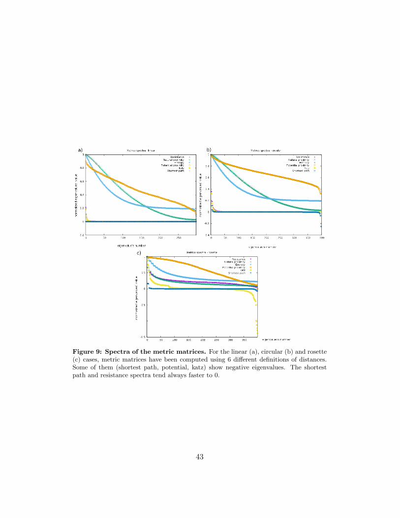
Figure 9: Spectra of the metric matrices. For the linear (a), circular (b) and rosette(c) cases, metric matrices have been computed using 6 different definitions of distances.Some of them (shortest path, potential, katz) show negative eigenvalues. The shortestpath and resistance spectra tend always faster to 0.

43

Figure 10: 3D Reconstruction of the simulated linear polymer. The graphs showthe reconstruction obtained by using the MDS with the (a) shortest path, (b) resistance,(c) proximity, (d) entropy, (e) potential and (f) katz distances.

44

Figure 11: 3D Reconstruction of the simulated circular polymer. The graphsshow the reconstruction obtained by using the MDS with the (a) shortest path, (b) resis-tance, (c) proximity, (d) entropy, (e) potential and (f) katz distances.

45

Figure 12: 3D Reconstruction of the simulated rosette polymer. The graphs showthe reconstruction obtained by using the MDS with the (a) shortest path, (b) resistance,(c) proximity, (d) entropy, (e) potential and (f) katz distances.

46

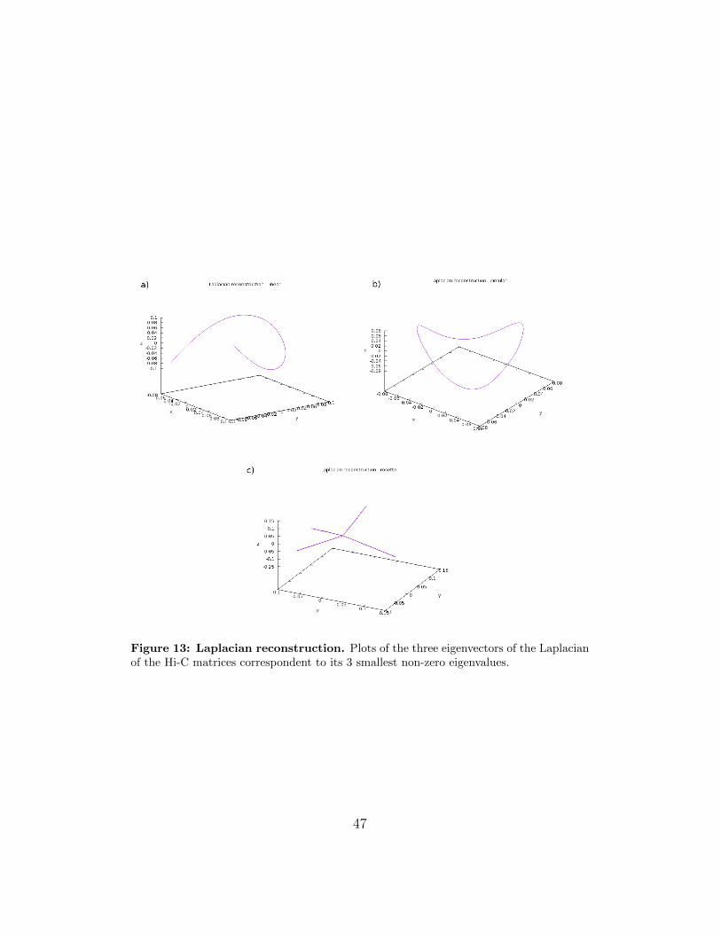
Figure 13: Laplacian reconstruction. Plots of the three eigenvectors of the Laplacianof the Hi-C matrices correspondent to its 3 smallest non-zero eigenvalues.

47

Figure 14: 2 dimensional plot of the circular simulation. The x and y axes of theshortest path reconstruction are plotted for the circular case.

the rank of the matrix is higher than in others, the projections of theconformation in a three dimensional space are still consistent with eachother;

• the potential proximity distance reconstruction doesn’t respect anyproperty of the polymer and of the reconstruction obtained by usingdirectly the simulated distance matrices;

• the entropy distance respects the symmetries but comparing it withthe natural proximity distance small perturbations arise. This is rea-sonable, thinking that the entropy proximity measure is computed asa perturbation of the natural proximity one due to the multiplicationof each entry of the matrix with its logarithm;

• in the rosette case, the Katz distance does not reproduce the samestructure of the others. This doesn’t happen in the linear and circularcase where its spectrum was non-negative;

• equally, in the circular case, even if the two dimensional plot is con-sistent with the other reconstructions (Fig. 14), the third eigenvector,correspondent to the third axes, is different.

In order to quantify these statements, we considered the reconstructedcoordinates vectors and we calculated the dot product with the correspond-ing coordinates previously obtained by using directly the simulated averageddistance matrix. The closer it is to 1 the more parallel the two vectors are,

48

hence the reconstruction is consistent with the expected structure.The resistance reconstruction is always consistent with a precision higherthan 93%. In the other cases the qualitative predictions of consistence areconfirmed. Some examples are shown in Fig. 15.

Hence, not all the reconstructions are consistent among themselves andnot all the reconstructions are consistent among the linear, circular androsette simulations.In order to explain this behavior, we show a reconstruction obtained by usingthe first three eigenvectors of the Laplacian of the graph instead (Fig. 13).Surprisingly, it is always consistent with the expected structure with a highprecision. The average structure over a high number of simulations is exactlyreproduced by the eigenmodes of the Laplacian of the contact-frequenciesweighted graph relative to the three smallest nonzero energy states.In the last years, the eigenvectors of the Laplacian have already been usedas a set of coordinates for the so-called synchronization dynamic of networks[39].From a theoretical point of view, it is possible to calculate the coordinateswith the MDS only using the resistance distance among the distances pro-posed in this thesis. In fact, as explained above, the first 3 eigenvectors ofits metric matrix are always the eigenvectors corresponding to the 3 smallestnonzero eigenvalues of the Laplacian. The resistance metric is the only onethat assures that the eigenvectors are the same and the order is reversed. Inthe other cases, even if we demonstrated that the Laplacian and the met-ric matrix share the same set of eigenvectors, their order is not said to berespected. In fact, in these cases it is not possible to predict how the eigen-values of the metric matrix depend from the Laplacian ones.

As an example, in the circular case the shortest path reconstruction didn’trespect the order of the eigenvectors of the Laplacian. Nevertheless, substi-tuting its third eigenvectors with its last one, the reconstruction would befully consistent with the expected one (Fig. 16).

Finally let’s note that according to the analogy of a system of springs con-necting the vertexes of the graph, the constant eigenmode of the Laplacianrepresents the case in which all the elongations are null and all the springsassume their equilibrium length, that is 0.

49

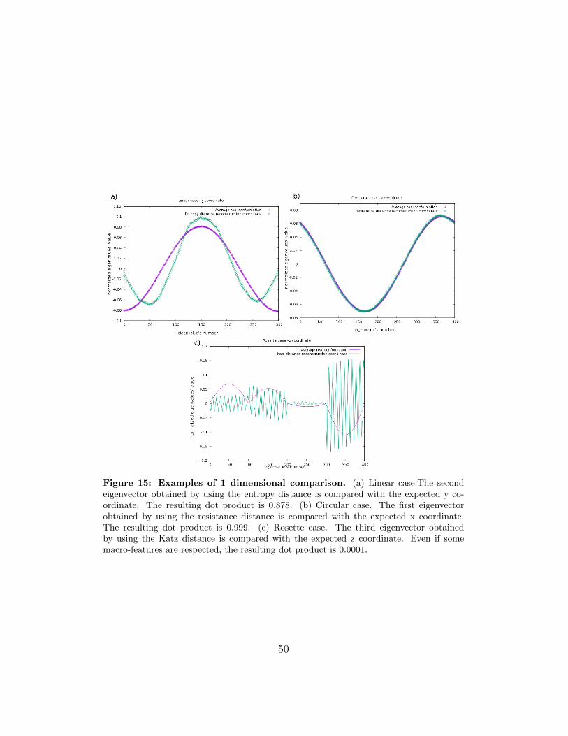
Figure 15: Examples of 1 dimensional comparison. (a) Linear case.The secondeigenvector obtained by using the entropy distance is compared with the expected y co-ordinate. The resulting dot product is 0.878. (b) Circular case. The first eigenvectorobtained by using the resistance distance is compared with the expected x coordinate.The resulting dot product is 0.999. (c) Rosette case. The third eigenvector obtainedby using the Katz distance is compared with the expected z coordinate. Even if somemacro-features are respected, the resulting dot product is 0.0001.

50

Figure 16: Example of different eigenvectors order. The plot shows the first,second and last eigenvector of the shortest path metric matrix in the circular case. Thedot product between the last eigenvector and the expected z axes is 0.998, but this doesn’tappear in the 3d reconstruction, since its correspondent eigenvalue is 0.

3.4 Real data

In this section we will apply the previously developed algorithms to a real setof Hi-C data. In fact, we verified that, simulating many times a self avoidingwalk for different shapes of a polymer, the average structure is reproducedby the first eigenvectors of the Laplacian of the related contact graph. Thisreconstruction is obtained by using the resistance distance in the multidi-mensional scaling technique.

In the experimental Hi-C data, usually a certain amount of different cellsis analyzed. They grow in common conditions and after a specific treatmentthey are subjected to formaldehyde fixation in order to create cross-links.The cross-links are then counted and finally the Hi-C matrix are created.Here we will apply the MDS to Hi-C data of the Bacillus subtilis [38] (Fig.17). Each analyzed cell contained one single and unreplicated chromosome.The genome has been divided into 1054 bins. The Hi-C data have beendemonstrated to be reproducible and consistent with the data obtained pre-viously.

Even in this case the resistance distance reconstruction has been demon-strated to be consistent with the first three eigenvectors of the Laplacian.In the past, some applications which use the shortest path distance havealready been proposed. MDS has been used in order to demonstrate the

51

Figure 17: Hi-C matrix. [Adapted from [38]] Hi-C contact matrix of the Bacillussubtilis. The white dashed box represents the situ in which the replication begins.

Figure 18: Laplacian spectrum. Spectrum of the Laplacian of the graph of theCaulobacter crescentus. Since there is only one 0 eigenvalue, the graph is connected.

52

Figure 19: Laplacian reconstruction. Plots of the three eigenvectors of the Laplacianof the Hi-C matrices correspondent to its 3 smallest non-zero eigenvalues.

Figure 20: Spectra of the metric matrices. Metric matrices have been computedusing 6 different definitions of distances. Some of them (shortest path, potential, katz)show negative eigenvalues.

53

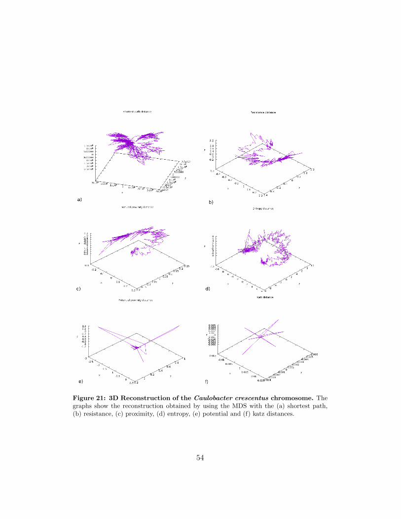
Figure 21: 3D Reconstruction of the Caulobacter crescentus chromosome. Thegraphs show the reconstruction obtained by using the MDS with the (a) shortest path,(b) resistance, (c) proximity, (d) entropy, (e) potential and (f) katz distances.

54

existence of particular domains and, in combination with super-resolutionmicroscopy, to verify that the structure of the chromosome changes duringthe life cicle of the cell [38]. In particular, it has been used to unveil thefactors responsible for its regulating folding. For further applications, thedifferent reconstruction obtained by using the resistance distance may revealother important features.

55

4 Other applications

4.1 Introduction

We have shown how it is possible to interpret the Hi-C data as an adjacencymatrix of a complete weighted graph and consequently reconstructing a setof three dimensional Euclidean coordinates. We showed in which cases thesecoordinates correspond to the first three eigenvectors of the Laplacian of thegraph. Nevertheless, this reconstruction unveils some overall properties ofthe chromosomes, carrying a loss of information about the local details ofthe structures, e.g. special patterns, loops or clusters.The following chapter will investigate an application of the method shownabove in the case in which distances between just a few pairs of points areknown with a certain precision. The reason of this request arises from somefluorescence measures that permit to visualize multiple loci at the same timeand hence to deduce their distances. Nevertheless, at the state of art it isnot possible to measure directly a complete set of distances.This thesis proposes two methods: the first one is a Bayesian method whosegoal is to use the Hi-C data in order to complete the fluorescence distancematrix or, in other words, it uses these distances as a constraint in the re-construction process; the second method asserts the uncertainty of the FISHdistances and uses them to reconstruct a new adjacency matrix of contactprobabilities that combine the two kinds of data.In our simulations we will consider as sets of measured distances a collectionof few distances chosen randomly from the previously used distance matrices,i.e. the one single conformation and the averaged distance matrix.

In both the methods we will stress the use of a probability density definedover some possible energy states that the graph can assume. The Boltzmannprobability density of the states of the generalized energy E of a graph G is:

ρ(E) = e−E = e12

∑ij d

2ijwij =

∏ij

e−12d2ijwij

Clearly, this probability density can change both with the frequencies wijand with the way the distances are defined. Some authors [2] have alreadyused this definition of probability density for graphs focusing on the way theprobability changes when the graph adjacency matrix is modified. In ourcases instead we will be interested on considering the energy value over all

56

the possible length that the distances can assume. For this purpose, thefollowing theorem on the number of independent distances will be useful.

Theorem. Given a set of N points in a d-dimensional space, the min-imal number of distances between the points that can be defined freely ism = d(d+1)

2+ (N − d− 1)(d+ 1) where d ≥ 2 and N ≥ 2.

Proof. The proof arises from symmetry considerations. Embedding N =d + 1 points needs necessarily

∑di=0 ni = d(d+1)

2lines. For any other point x

added are then necessary d + 1 lines in order to not have any other degreeof freedom. In fact, adding only d lines from x to other d points, then thesepoints form a d-dimensional surface such that x can assume two different sym-metric positions respect of the surface itself. Hence all the distances of x withthe other points would change. Thus, it is necessary to add (N−d−1)(d+1)distances.

By this demonstration it is clear that the choice of the m distances is notarbitrary. For instance, in the three dimensional case we must define for eachpoint at least 4 distances with other points.For a three dimensional space at least only m = 4N − 10 distances can befreely chosen. Fixing them the other ones will be certain. Let d denote theset of some m′ independent distances, where m′ ≤ m. Then we define apartition function Z ′ of the graph as

Z ′ =

∫ ∞0

e−E(d)dm′d =

=m′∏

(ij)=1

∫ ∞0

e−12d2(ij)

w(ij)dd(ij) =

=

(√π

2

)m′ (m′)∏(ij)=1

1√w(ij)

where in the last step we used the Gaussian integral.

57

4.2 Bayesian method

The following method’s goal is to modify the adjacency matrix W of theHi-C data inserting an additional information. This means assuming thata set of M distances d∗ is known from a statistical point of view. In fact,we can interpret the entries wij of W as the probability p(ij) that there is acontact between the points i and j, i.e. their distance dij = 0.Considering the additional information provided by d∗ means calculatingp(ij|d∗). Using the Bayes theorem:

p(ij|d∗) =p(ij)p(d∗|ij)

p(d∗)= p(d∗|ij)wij

provided that p(d∗) = 1 and d∗ > 0.By definition, p(d∗|ij) = 0 whenever one of the distances of d∗ is the distancebetween the points i and j. Let’s assume the case in which d(ij) = 0 /∈ d∗

and let d denote all the independent distances not belonging to d∗. They willconsequently be m−M . Then:

p(d∗|ij) =e−E(d)e−E(d∗)

Z∗

In this case, the partition function Z∗ is calculated integrating the proba-bility density not over all the independent distances, but only between thedistances d∗. In fact, in this case we are interested on calculating it only overthe values that the experimental measure could assume. Hence:

p(d∗|ij) =e−E(d)e−E(d∗)

e−E(d)∫∞0e−E(d∗)dd∗

=

√2

π

M

e−E(d∗)∏M

√wM

Consequently:

w′ij = p(ij|d∗) = wij

√2

π

M

e−E(d∗)∏M

√wM

Hence, these assumptions yield to the multiplication of the adjacency matrixwith a constant factor, always smaller than 1. The entries corresponding tothe given set of distances are set to 0. Considering the set of N points asconnected by springs with elastic constant equal to the contact frequency,

58

Figure 22: Substitution of one single distance. One defined and consistent, but raredistance has been imposed to the circular structure. The number of consistent distancesis low and it doesn’t show any interesting property.

then setting one of them to 0 means substituting the spring with a not de-formable bar of fixed length.The new adjacency matrix has to be newly normalized in order to let therows and the columns sum again to 1.Even if the method is theoretically interesting, it can not find immediateapplications. Its principal defect is that the measured distance is appliedduring a second step of the algorithm and this may not be consistent. Infact, applying the reconstruction method to the new adjacency matrix doesnot assure that the distances between two points - whose distance is supposedto be d∗ - will be exactly d∗. This condition should be imposed a posteriori,provided that d∗ is consistent with the distances calculated, i.e. it satisfiesthe triangular inequality with any other third point. This case is really rareand, even if applied, it doesn’t yield to any interesting result (see Fig. 22).

4.3 New frequency method

We showed some limitations of the previous problem. In particular, it is notpossible to be sure a priori that the measured distance is consistent with thereconstruction. Furthermore, we didn’t take into account the uncertainty ofthe measured distance. In fact, one may assert that the measured distanceis not certain, but it is the most probable among all the possible values itcan take. The following method arises from this assumption.

59

We will find a way to redefine the entries of the adjacency matrix. For thispurpose, let’s assume that each measured distance d∗ is equal to the averagedistance that we would obtain by using the probability density ρ(E). Thatis, consider

d∗ =

√〈d1〉2 + 〈d2〉2 + · · ·+ 〈dN〉2

where the average of each component of the distance is

〈di〉 =

∫∞0λidie

−E(d)dd1 . . . dd4N−10∫∞0e−E(d)dd1 . . . dd4N−10

=

∫∞0die− 1

2λid

2iwddi∫∞

0e−

12λid2iwddi

=

√2

π

√λi√w

Hence the distance is:

d∗ =

√2

π

1√w

√∑i

λi

Consequently, we can compute the related frequency of contact between twopoints i and j as:

wij =2

π

1

d∗2ijTrM

This definition can be interpreted as a constraint for the energy of the graph,since wijd

∗2ij is dimensionally equivalent to the energy itself.

Let’s note that, since the relative frequency can’t be bigger than 1, then

the measured distance should be rescaled in such a way that d∗ ≥√

2πTrM

.

This means considering a rescaled distance: d∗resc =

√2/(πTrM)

d∗mind∗ where d∗min

is the smallest value that experimentally d∗ can assume. Alternatively, it ispossible to define arbitrarily a threshold distance d∗min, imposing that for anydistance d∗ij ≤ d∗min, then wij = 1. This means that the new probability wijdoes not depend on the constant factor 2TrM

π, but only on the choice of the

threshold distance.After the substitution of the new few entries, it will be necessary to re-normalize the matrix with the Sinkhorn-Knopp algorithm [50], in order tolet each row and column sum to 1. In fact, by construction the probabilitiesthat we found are the probabilities of uncorrelated events: the sum of differ-ent probabilities in the same row may be bigger than 1. The normalizationassures that the contacts are considered mutually exclusive events; the rescal-ing of the distances assures that the new frequency are in any case consistentwith the dimensions of the structure of the polymer. The normalization lets

60

Figure 23: Reconstruction of the average structure. The algorithm of the newfrequencies has been applied to the linear (a), circular (b) and rosette (c) structures usingall the distances of the matrices of the averaged distances used also previously.

the new and the old data influence each other.In order to verify the consistence of this construction we first reconstructedthe conformation of the polymers, substituting all the entries of the adja-cency matrices with the new frequencies, using the averaged distance thatwe have already used before (Fig. 7 a,c,e). Then, we applied the resistancedistance MDS algorithm to obtain the three dimensional reconstruction. Thethreshold distance of the rescaling has been fixed as the maximum distancebetween two consecutive monomers in the simulated chain.The results and the spectra of the metric matrices are shown in Fig. 24 and23.

Computing the dot product of the original coordinates vectors with the

61

Figure 24: Spectra of the reconstruction of the average structure. The shownspectra are the spectra of the metric matrices of the reconstruction with the new frequen-cies applied to the linear (a), circular (b) and rosette (c) structures using all the distancesof the matrices of the averaged distances used also previously.

62

correspondent reconstructed ones, they are verified to be exactly parallel.Consequently, they are parallel to the coordinates vector obtained by usingthe simulated Hi-C matrices. This result is reasonable. In fact the distancesare averaged over a high number of simulation. The smaller the average dis-tance, the higher the amount of small distances and the higher the frequencyof contact too, according to the definition of frequencies used to calculate theHi-C matrices.Consequently, we substituted only 100 frequencies on the adjacency matrix,using only 100 random distances of the previously used set. The shape of thestructure results in any case slightly perturbed, probably due to the renor-malization process (Fig. 25).

Therefore, the algorithm has been applied not to the average distances,but to the distances among the points of the particular singular conforma-tions shown in Fig. 7 b, d, f. Even in this case the threshold distance usedto rescale the distances is the maximum distance between two consecutivemonomers of the chain. The spectra and the reconstructions are shown inFig. 27 and 26.

The reconstruction is now not exactly consistent with the original one.Table 2 shows the values of the dot products between the correspondent axes.The first axes result parallel with high precision. The precision is lower forthe second axis, but still high, and finally it is not always acceptable forthe third axis. Since many of the eigenvalues are different than 0, the recon-struction is a projection on the first three coordinates of a higher dimensionalspace. In the original reconstruction the rank of the metric matrix was in-stead exactly 3 since the set of distances was directly computed in a threedimensional space (Fig. 6). The inconsistency now arises from the errorsintroduced with the indirect computation of the distance through a contacts’frequency matrix.Let’s note that in the average structure’s case the reconstruction is consistentsince the spectrum of the metric matrix was already smoothed in the originalreconstruction.

Finally, we substituted only 20, 100 and 1000 new frequencies to theadjacency matrix of the simulated Hi-C data corresponding to the averagestructure. This test was performed in order to show how the structure in-creasingly changes when new distances are added. The change of the struc-

63

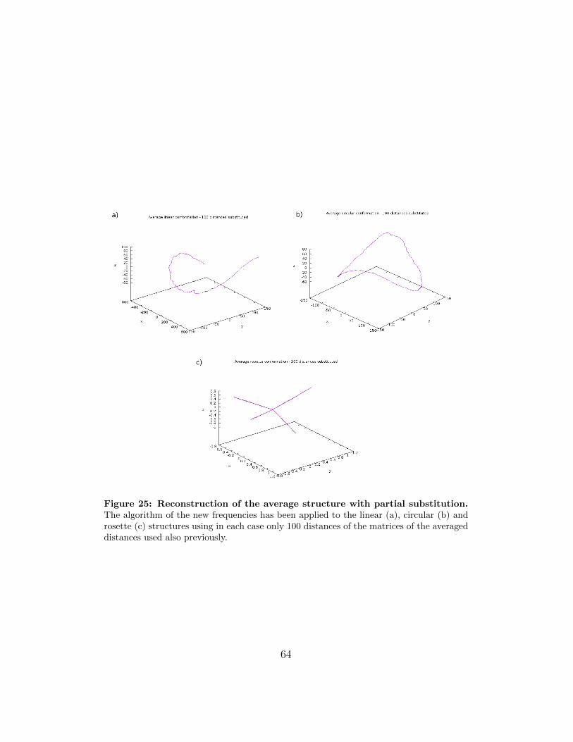
Figure 25: Reconstruction of the average structure with partial substitution.The algorithm of the new frequencies has been applied to the linear (a), circular (b) androsette (c) structures using in each case only 100 distances of the matrices of the averageddistances used also previously.

64

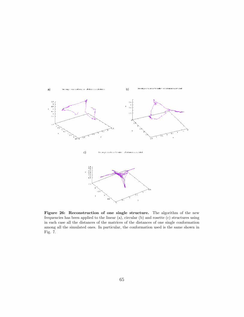
Figure 26: Reconstruction of one single structure. The algorithm of the newfrequencies has been applied to the linear (a), circular (b) and rosette (c) structures usingin each case all the distances of the matrices of the distances of one single conformationamong all the simulated ones. In particular, the conformation used is the same shown inFig. 7.

65

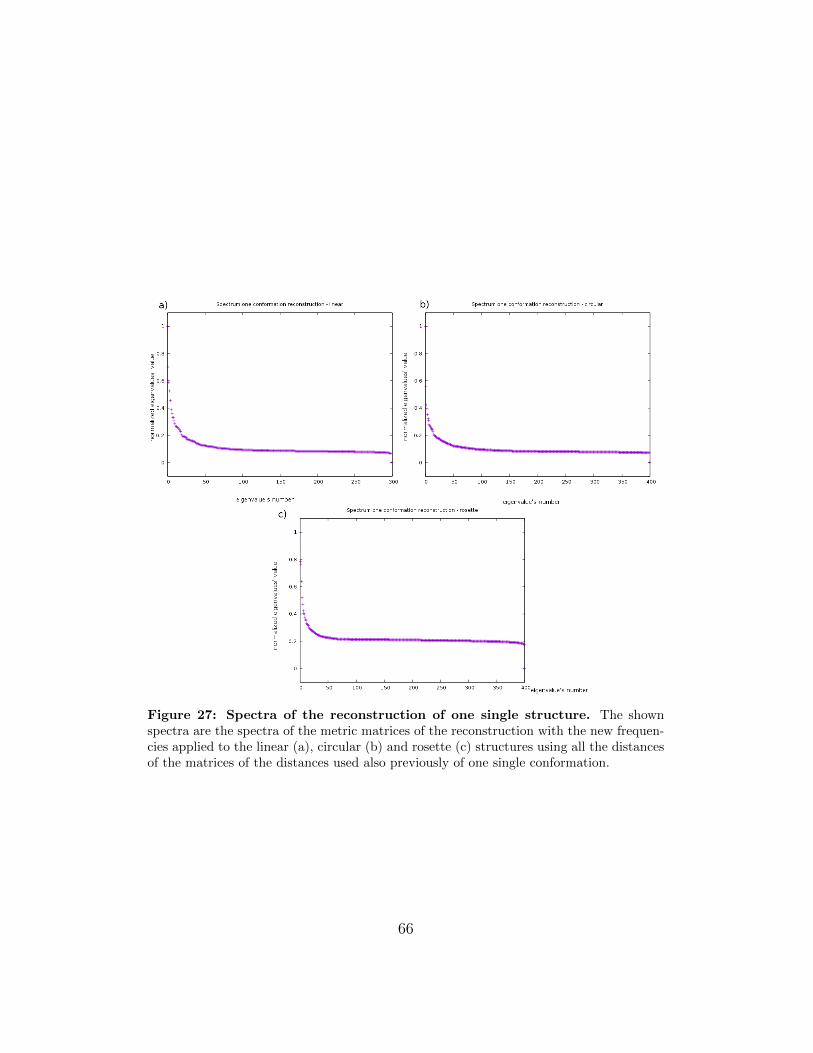
Figure 27: Spectra of the reconstruction of one single structure. The shownspectra are the spectra of the metric matrices of the reconstruction with the new frequen-cies applied to the linear (a), circular (b) and rosette (c) structures using all the distancesof the matrices of the distances used also previously of one single conformation.

66

x y z

Linear 0.973 0.874 0.812Circular 0.992 0.705 0.551Rosette 0.985 0.881 0.457

Table 2: Dot products between reconstructed and real coordinates. The theo-retical value of the dot product for parallel vectors is 1. Here are shown the dot productsbetween the real coordinates’ vector and the ones reconstructed through the use of thenew frequencies. The dot product decreases with the order of the axes.

ture is continuous and in each case deforms the average structure withoutbreaking it, i.e. there are not points in isolated areas, not belonging to thestructure (Fig. 28, 29, 30).

The method presented in this last chapter has been proposed in orderto combine two different sets of data: one consisting of contact frequencies(Hi-C data) and one consisting of a set of few directly measured distances.We showed that if the set of measured distances is complete it is possible toreconstruct a second probabilities matrix analogous to the Hi-C matrix. Thetwo matrices are consistent only if the set of distances coincides with the av-erage distances over all the conformations analyzed by the Hi-C method. Inthe other cases, we obtained some reconstructions whose precision decreaseswith the order of the coordinates. Then we only changed some frequencieson the Hi-C matrix through the new algorithm showing that the structureslightly changes increasing the number of new frequencies, but always in asmooth way.This technique is obviously not accurate enough, but it presents some inter-esting properties. Relationships between the spectra of the metric matricesand on the choice of a particular set of distances may be further analyzed inorder to understand the behavior of the reconstruction.

67

Figure 28: Reconstruction of the linear structure with partial substitution. Thealgorithm of the new frequencies has been applied to the linear structure using only (a)20, (b) 100 or (c) 1000 distances of the matrix of the distances of one single conformationamong all the simulated ones. In particular, the conformation used is the same shown inFig. 7.

68

Figure 29: Reconstruction of the circular structure with partial substitution.The algorithm of the new frequencies has been applied to the circular structure usingonly (a) 20, (b) 100 or (c) 1000 distances of the matrix of the distances of one singleconformation among all the simulated ones. In particular, the conformation used is thesame shown in Fig. 7.

69

Figure 30: Reconstruction of the rosette structure with partial substitution.The algorithm of the new frequencies has been applied to the rosette structure usingonly (a) 20, (b) 100 or (c) 1000 distances of the matrix of the distances of one singleconformation among all the simulated ones. In particular, the conformation used is thesame shown in Fig. 7.

70

5 Conclusions

In this thesis, we investigated the structure of chromosomes, the moleculesthat carry all the genetic information of a living being. In fact, high orderstructural features may be connected with their function and with the geneexpression. Despite its importance, at the state of the art there is not atechnique to measure the coordinates or the distances between the loci of achromosome directly and with high resolution. In the last years, CapturingChromosome Conformation (3C) first and Hi-C later provided a method toobtain a genomewide topological information at high resolution.In particular, the data consist in matrices of relative frequencies of contactbetween the loci. The goal of this thesis was to interpret this data in such away to obtain a three dimensional reconstruction of the chromosome. Thishas been performed by means of the interpretation of the Hi-C matrix as theadjacency matrix of a weighted complete undirected graph. Therefore it waspossible to define distances between the vertexes of the graph. We proposeddifferent definitions of distances in graphs. In particular, we focused on theshortest path, resistance, natural proximity, entropy, potential proximity andKatz distances.By defining these distances between the nodes of the graph - correspond-ing to the loci of the chromosome - we applied the Multidimensional scalingmethod in order to reconstruct the Euclidean coordinates.Multidimensional scaling consists of generating a Gram or metric matrix Mfrom the distance matrix. We showed that a necessary and sufficient con-dition to embed N points with the given distances in an Euclidean spaceof dimension r is M to be of rank r and semi-definite positive. The recon-structed coordinates’ vector will be parallel to the eigenvectors of the metricmatrix. If r ≥ 3 we can reconstruct a projection in the first three coordinates.

Therefore, we simulated Hi-C data for three different polymers with alinear, circular and rosette shape. We calculated all the distance matricesfor all of them and we applied the MDS for each of these distances. Thereconstructed structures were not always equal each other and not alwaysconsistent with the expected structure. This has been calculated applyingMDS to the average distances of all the simulated conformations.The only distance whose reconstruction is always consistent is the resistancedistance. Considering the Laplacian matrix L of the graph and a set of coor-dinates composed by its three eigenvectors corresponding to the lowest three

71

non zero eigenvalues, we obtain a reconstruction always consistent with theexpected average structure of the polymers.Any metric matrix that commutes with L, share with it a common eigenvec-tor basis. The shortest path, resistance, proximity and Katz distances yieldto this property. Among them, the resistance distance is the only one thatprovides the same reconstruction of the Laplacian eigenvectors. In fact, sinceits eigenvalues are the inverse of the Laplacian eigenvalues, the order of theeigenvectors is reversed.We applied these algorithms to a set of real data too, obtaining further re-constructions.

Finally, we considered the problem of combining the Hi-C data with somedistances directly measured with the fluorescence technique. For this pur-pose, we introduced a partition function on the energetic states that a graphcan assume. Using it with a Bayesian approach, it is possible to modifythe adjacency matrix and obtain a new reconstruction. Nevertheless, thismethod is not said to respect a priori the measured distances given as con-straints.Instead, forcing the measured distance to be the average distance obtainedby means of the partition function, we found a quadratic inverse relation-ship between a measured distance and its corresponding contact frequency.As expected, using the complete set of average distances, this relationshipis perfectly consistent with the expected average structure. Using the set ofdistances of one single conformation, the reconstruction is excellent for thex axis, but registers a lack of precision in the y and z axes. This is probablydue to the average operation. We showed that this reconstruction modifiessmoothly the shape of the polymer increasing the number of measured dis-tances in the experiment. The insertion of only one new frequency influenceseven the other frequencies and the structure changes slightly. The recon-struction is not accurate enough, but it definitely suggests a basic methodfor further studies.

The goal of this thesis was to describe some theoretical basis on themultidimensional scaling process and on the application of this method ingraphs. For this purpose we investigated the ways to define distances ongraphs, their relationships with the Laplacian matrix and the conditions toembed the graph in an Euclidean space. During the work, many similaritieswith other physics fields have been underlined. Spectral graph theory is in

72

fact generally applicable to many areas. In this case the energy levels ofthe Laplacian have been interpreted as conditions for a three dimensionalreconstruction of chromosomes. Further studies may continue to focus onthis interpretation and on similar applications.In fact, the study of chromosomes’ structure is fundamental in biology and inmedicine. It may unveil its relationship with chromosomes functionality or,in the worst case, its relationship with its dysfunctional role. In other words,it is important in order to understand the mechanisms of the transmissionof life, that is finally the reason why we do research.

73

6 Appendix A

Given a complete set of distances between N points, the embedding problemconsists in understanding when the given distances are Euclidean, i.e. whenit is possible to find some Cartesian coordinates in a generic r-dimensionalspace (r ≤ N). The following theorem establishes the minimum value of rand the necessary and sufficient conditions to embed the set of points.

Theorem. [47] A necessary and sufficient condition that the Dij be thelengths of the edges of an n-”simplex” lying in Rr but not in Rr−1 is thatthe quadratic form

F (x1, . . . xn) =1

2

∑i,j

(d20i + d20j −D2ij)xixj

be positive ( i.e. always ≥ 0) and of rank r. That is, the associate matrixM has to be positive semidefinite of rank r.

Proof. Necessity. Let r0 = 0 be the origin of an Euclidean space in whichri are the coordinates of the i-th point. Considering a point P such that

rP = x1r1 + · · ·+ xnrn

its distance from the barycenter is:

d20P =∑i

x2i∑ν

r2iν + 2∑i<k

xixk∑ν=1

riνrkν

Since: ∑i

x2i∑ν

r2iν =∑i

x2i r20i = 0

and:

2∑ν

riνrkν =∑ν

r2iν +∑ν

r2kν −∑ν

(riν − rkν)2 = d20i + d20j −D2ij

we have d20p = F (x1 . . . xn). Hence F is positive. Furthermore, P = F = 0on a linear manifold of n − r dimensions in the variables x1 . . . xn, hence Fis of rank r.Sufficiency. Let us assume F to be positive definite, i.e. r = n. By means

74

of a certain linear non singular transformation y = H(x) we get F = y21 +· · · + y2n. Let’s consider the Cartesian space of the variables (y1, . . . yn) andn correspondent points whose coordinates are:

(x1, . . . xn) = (1, 0, . . . 0), (0, 1, . . . 0), . . . , (0, 0, . . . 1)

Their coordinates are found by y = H(x), for their mutual distances we find:

x0xi2 = F (0, . . . 1 . . . 0) = d20i

xixj2 = F (0, . . . 1 · · · − 1 . . . 0) = d20i + d20k − (d20i + d20k − d2ik) = d2ik

Hence, these are exactly the coordinates we are looking for. If r < n thenF (x1 . . . xn) = y21 +y22 + · · ·+y2r and the distances d20i and d2ij are the squaredlengths of the projections on the sub-space (y1 . . . yn), i.e. on a manifoldyr+1 = · · · = yn = 0. By construction the n-simplex of points we found iscontained in a Rr but not in Rr−1.

75

7 Appendix B

Algorithms and codes.The following algorithms are coded in language C++. We stressed the useof the template library Eigen [25], projected for linear algebra calculus. Itallowed us to deal with matrices of high dimension and to compute quicklytheir spectral decomposition.The input of any MDS algorithm is the Hi-C matrix. It is declared asweight(N,N) where N is the dimension of the matrix. In the following tableswe show the algorithms to calculate the 6 distances matrices dist(N,N) usedin the ”Results” chapter from the weight(N,N) matrix.We defined two Eigen types as follows:

typedef Matrix<long double, Dynamic, Dynamic> stdmat;

typedef Matrix<long double, 1, Dynamic> stdvec;

Shortest path.

long double eps=1e-20;

for (int i=0; i <N; i++) {

for (int j=0; j <N; j++){

if (abs(weight(i, j)) > eps)

weight(i, j)=1./weight(i, j);

if (abs(weight(i, j)) < eps)

weight(i, j)=1e308; } } //theoretically infinity

for (int i=0; i<N; i++){

for (int j=0; j<N; j++){

dist(i, j)=weight(i, j);

} }

for(int i=0; i<N; i++){

dist(i,i)=0.;

}

int correct=1;

while(correct != 0){

//we iterate until all points respect the triangle inequality (correct=0)

correct=0;

76

for(int i=0; i<N;i++){

for(int j=0; j<N;j++){

for(int k=0;k<N;k++){

if( ( dist(i, j)>( dist(i, k)+dist(k, j) ) )

&& (abs(dist(i, k))>eps) && (abs(dist(k, j))>eps) ) {

dist(i, j)=dist(i, k)+dist(k, j);

dist(j,i)=dist(i,j);

} } } }

for(int i=0; i<N;i++){

for(int j=0; j<N;j++){

for(int k=0;k<N;k++){

if( ( dist(i, j)>(dist(i, k)+dist(k, j)) )

&& (abs(dist(i, k))>eps)

&& (abs(dist(k, j))>eps)) {

correct++;

} } } } } }

Resistance.

// Calculus of the Laplacian matrix

stdvec rows(N);

for (int i=0; i<N; i++){

rows(i)=0.;

}

for (int i=0; i<N; i++){

for (int j=0; j<N; j++){

rows(i)=rows(i)+weight(i,j);

} }

for (int i=0; i<N; i++){

for (int j=0; j<N; j++){

weight(i,j)=-weight(i,j);

} }

for(int i=0; i<N;i++){

weight(i,i)=rows(i); }

77

for (int i=0; i<N; i++){

for (int j=0; j<N; j++){

weight(i,j)=weight(i,j)+1./N;

}

}

weight = weight.inverse();

for (int i=0; i<N; i++){

for (int j=0; j<N; j++){

weight(i,j)=weight(i,j)-1./N;

}

}

for (int i=0; i<N; i++){

for (int j=0; j<N; j++){

dist(i, j)=weight(i, i)+weight(j,j)-2*weight(i,j);

} }

Natural proximity.

stdvec rows(N);

for (int i=0; i<N; i++){

rows(i)=0.;

}

for (int i=0; i<N; i++){

for (int j=0; j<N; j++){

if( i!= j){

rows(i)=rows(i)+weight(i,j);

}} }

stdmat prox(N,N); //proximity matrix

for(int i=0; i<N;i++){

for(int j=0; j<N; j++){

if (i != j){

prox(i,j)=weight(i,j); }

if (i == j){

prox(i,j)=rows(i);}

78

} }

//Does it respect the proximity properties?

int triangle =0;

for (int i=0; i<N; i++) {

for (int j=0; j<N; j++){

if ( abs(prox(i,j) -prox(j,i))>eps) {

cout << "Error symmetry " << i << "," << j << endl;}

if ( prox(i,i) < prox(j,i) ) {

cout << "Error maxim diagonal: " << i << "," << j << endl;}

if ((prox(i,j))<0) {

cout << "Error negative: " << i << "," << j << endl;}

for(int k=0; k<N; k++) {

if ((prox(i,j)+prox(i,k)-prox(j,k))>prox(i,i) && i != j && i!= k){

cout << i << " " << j << " " << k << endl;

triangle++;}}

} }

cout << "Triangle = " << triangle << endl;

stdmat dist(N,N); // distance matrix

for (int i=0; i<N; i++){

for (int j=0; j<N; j++){

dist(i, j)=prox(i,i)+prox(j,j)-2*prox(i,j);

} }

Entropy distance.

for (int i=0; i<N; i++){

for (int j=0; j<N; j++){

if (abs(weight(i,j))> eps) {

weight(i,j)= -weight(i,j)*log(weight(i,j));

}

if (abs(weight(i,j))< eps) { weight(i,j)=0.;}

} }

stdvec rows(N);

for (int i=0; i<N; i++){

rows(i)=0.;

79

}

for (int i=0; i<N; i++){

for (int j=0; j<N; j++){

if( i!= j){

rows(i)=rows(i)+weight(i,j);

} } }

stdmat prox(N,N); //proximity matrix

for(int i=0; i<N;i++){

for(int j=0; j<N; j++){

if (i != j){

prox(i,j)=weight(i,j); }

if (i == j){

prox(i,j)=rows(i);}

} }

\\Check if it verifies the proximity properties as done before

for (int i=0; i<N; i++){

for (int j=0; j<N; j++){

dist(i, j)=prox(i,i)+prox(j,j)-2*prox(i,j);

} }

The potential proximity distance is analogous.Katz distance.

for(int i=0;i<N;i++){

for(int j=0;j<N;j++){

weight(i,j)=-weight(i,j);

}

}

for(int i=0;i<N;i++){

weight(i,i)=1;

}

weight = weight.inverse();

for(int i=0;i<N;i++){

weight(i,i)=weight(i,i)-1;

}

80

stdvec rows(N);

for (int i=0; i<N; i++){

rows(i)=0.;

}

for (int i=0; i<N; i++){

for (int j=0; j<N; j++){

rows(i)=rows(i)+weight(i,j);

}

}

stdmat dist(N,N); //minimum path distance matrix

for (int i=0; i<N; i++){

for (int j=0; j<N; j++){

dist(i, j)=weight(i, i)+weight(j,j)-2*weight(i,j);

} }

For each of these distance matrices we applied the MDS algorithm:

stdvec somma(N);

somma.setZero();// useful on the calculation of the barycenter distance

long double somma2 = 0.;

stdvec distbaryc(N);

distbaryc.setZero();//distances from the barycenter

for (int i=0; i<N; i++){

for (int j=0; j<N; j++){

somma(i)=somma(i)+dist(i, j)*dist(i, j);

}

}

for (int j=0; j<N; j++){

for (int k=0; k<j+1; k++){

somma2=somma2+dist(j, k)*dist(j, k);

}

}

for (int i=0; i < N; i++) {

distbaryc(i)=somma(i)/N - somma2/(N*N);

81

if (distbaryc(i) < 0)

distbaryc(i)=0.;

}

stdmat gram(N,N); //Gram or metric matrix

for (int i=0; i<N; i++){

for (int j=0; j<N; j++){

gram(i, j)=(distbaryc(i)+distbaryc(j)-dist(i, j)*dist(i, j))/2.;

} }

EigenSolver<stdmat> es;

es.compute(gram, true);

stdvec eigenval = es.eigenvalues().real();

stdmat eigenvec = es.eigenvectors().real();

stdmat coord(N,N);

long double eigenvalues[N];

int neg=0;

for (int i=0; i < N; i++) {

eigenvalues[i]=eigenval(i); }

//ordering the eigenvalues and the eigenvectors

long double temp=10.;

long double temp2=10.;

int m=0;

while(m<N-1){

if( eigenvalues[m] < eigenvalues[m+1] ) {

temp=eigenvalues[m];

eigenvalues[m]=eigenvalues[m+1];

eigenvalues[m+1]=temp;

for (int j=0; j<N; j++){

temp2=eigenvec(j, m);

eigenvec(j, m)=eigenvec(j,m+1);

eigenvec(j, m+1)=temp2;

}

m=0;

82

}

else

m++;

}

//calculate the coordinates

for (int i=0; i<N; i++){

if(eigenvalues[i]<0.){

eigenvalues[i]=0.;} // set to zero the negative eigenvalues

for (int j=0; j<N; j++){

coord(i, j)=eigenvec(j, i)*((eigenvalues[i]));

} }

83

References

[1] Erik D Andrulis, Aaron M Neiman, David C Zappulla, and RolfSternglanz. Perinuclear localization of chromatin facilitates transcrip-tional silencing. Nature, 394(6693):592–595, 1998.

[2] Rolf Backofen, Markus Fricke, Manja Marz, Jing Qin, and Peter FStadler. Distribution of graph-distances in boltzmann ensembles ofrna secondary structures. In International Workshop on Algorithms inBioinformatics, pages 112–125. Springer, 2013.

[3] Mikhail Belkin and Partha Niyogi. Laplacian eigenmaps and spectraltechniques for embedding and clustering. In NIPS, volume 14, pages585–591, 2001.

[4] Marek Biskup. On the scaling of the chemical distance in long-rangepercolation models. Annals of Probability, pages 2938–2977, 2004.

[5] G. Caldarelli. Scale-free networks: complex webs in nature and technol-ogy. Oxford University press, 2007.

[6] I Carmesin and Kurt Kremer. The bond fluctuation method: a new ef-fective algorithm for the dynamics of polymers in all spatial dimensions.Macromolecules, 21(9):2819–2823, 1988.

[7] Pavel Chebotarev. A class of graph-geodetic distances generalizing theshortest-path and the resistance distances. Discrete Applied Mathemat-ics, 159(5):295–302, 2011.

[8] Pavel Chebotarev. The graph bottleneck identity. Advances in AppliedMathematics, 47(3):403–413, 2011.

[9] Pavel Chebotarev and Elena Shamis. Matrix-forest theorems. arXivpreprint math/0602575, 2006.

[10] Pavel Chebotarev and Elena Shamis. On proximity measures for graphvertices. arXiv preprint math/0602073, 2006.

[11] Jie Chen and Ilya Safro. Algebraic distance on graphs. SIAM Journalon Scientific Computing, 33(6):3468–3490, 2011.

84

[12] Fan RK Chung. Spectral graph theory, volume 92. American Mathemat-ical Soc., 1997.

[13] Daniel M Cimbora and Mark Groudine. The control of mammalian dnareplication: a brief history of space and timing. Cell, 104(5):643–646,2001.

[14] Ewan R Colman and Nathaniel Charlton. Separating temporal andtopological effects in walk-based network centrality. Physical Review E,94(1):012313, 2016.

[15] Thomas Cremer and Christoph Cremer. Chromosome territories, nu-clear architecture and gene regulation in mammalian cells. Nature re-views genetics, 2(4):292–301, 2001.

[16] GORDON M Crippen and Timothy F Havel. Stable calculation of co-ordinates from distance information. Acta Crystallographica Section A:Crystal Physics, Diffraction, Theoretical and General Crystallography,34(2):282–284, 1978.

[17] Job Dekker, Karsten Rippe, Martijn Dekker, and Nancy Kleckner. Cap-turing chromosome conformation. science, 295(5558):1306–1311, 2002.

[18] MV Dhanyamol and Sunil Mathew. Distances in weighted graphs. An-nals of Pure and Applied Mathematics, 8(1):1–9, 2014.

[19] Jesse R Dixon, Siddarth Selvaraj, Feng Yue, Audrey Kim, Yan Li, YinShen, Ming Hu, Jun S Liu, and Bing Ren. Topological domains inmammalian genomes identified by analysis of chromatin interactions.Nature, 485(7398):376–380, 2012.

[20] Ivan Dokmanic, Reza Parhizkar, Juri Ranieri, and Martin Vetterli. Eu-clidean distance matrices: essential theory, algorithms, and applications.IEEE Signal Processing Magazine, 32(6):12–30, 2015.

[21] Leon Festiger. The analysis of sociograms using matrix algebra. Humanrelations, 1949.

[22] Robert W Floyd. Algorithm 97: shortest path. Communications of theACM, 5(6):345, 1962.

85

[23] LR Ford Jr and DR Fulkerson. Maximal flow through a network. InClassic papers in combinatorics, pages 243–248. Springer, 2009.

[24] John Clifford Gower. Euclidean distance geometry. Math. Sci, 7(1):1–14,1982.

[25] Gael Guennebaud, Benoıt Jacob, et al. Eigen v3.http://eigen.tuxfamily.org, 2010.

[26] Ivan Gutman. The energy of a graph: old and new results. In Algebraiccombinatorics and applications, pages 196–211. Springer, 2001.

[27] Timothy F Havel, Irwin D Kuntz, and Gordon M Crippen. The theoryand practice of distance geometry. Bulletin of Mathematical Biology,45(5):665–720, 1983.

[28] Donald B Johnson. Efficient algorithms for shortest paths in sparsenetworks. Journal of the ACM (JACM), 24(1):1–13, 1977.

[29] Leo Katz. A new status index derived from sociometric analysis. Psy-chometrika, 18(1):39–43, 1953.

[30] Douglas J Klein and Milan Randic. Resistance distance. Journal ofMathematical Chemistry, 12(1):81–95, 1993.

[31] Philip A Knight. The sinkhorn-knopp algorithm: convergence and appli-cations. SIAM Journal on Matrix Analysis and Applications, 30(1):261–275, 2008.

[32] Allen Knutson and Terence Tao. Honeycombs and sums of hermitianmatrices. Notices Amer. Math. Soc, 48(2), 2001.

[33] Peter Kuchment. Quantum graphs: an introduction and a brief survey.arXiv preprint arXiv:0802.3442, 2008.

[34] Tung BK Le, Maxim V Imakaev, Leonid A Mirny, and Michael T Laub.High-resolution mapping of the spatial organization of a bacterial chro-mosome. Science, 342(6159):731–734, 2013.

[35] Annick Lesne, Julien Riposo, Paul Roger, Axel Cournac, and JulienMozziconacci. 3d genome reconstruction from chromosomal contacts.Nature methods, 11(11):1141–1143, 2014.

86

[36] Bruno Levy. Laplace-beltrami eigenfunctions towards an algorithmthat” understands” geometry. In IEEE International Conference onShape Modeling and Applications 2006 (SMI’06), pages 13–13. IEEE,2006.

[37] Erez Lieberman-Aiden, Nynke L Van Berkum, Louise Williams, MaximImakaev, Tobias Ragoczy, Agnes Telling, Ido Amit, Bryan R Lajoie,Peter J Sabo, Michael O Dorschner, et al. Comprehensive mapping oflong-range interactions reveals folding principles of the human genome.science, 326(5950):289–293, 2009.

[38] Martial Marbouty, Antoine Le Gall, Diego I Cattoni, Axel Cournac,Alan Koh, Jean-Bernard Fiche, Julien Mozziconacci, Heath Murray,Romain Koszul, and Marcelo Nollmann. Condensin-and replication-mediated bacterial chromosome folding and origin condensation revealedby hi-c and super-resolution imaging. Molecular cell, 59(4):588–602,2015.

[39] Patrick N McGraw and Michael Menzinger. Laplacian spectra as adiagnostic tool for network structure and dynamics. Physical Review E,77(3):031102, 2008.

[40] Efe A. Ok. Real Analysis with Economic Applications. Princeton Uni-versity press, 2011.

[41] Beresford N Parlett. The symmetric eigenvalue problem, volume 7.SIAM, 1980.

[42] Roger Penrose. A generalized inverse for matrices. In Mathematicalproceedings of the Cambridge philosophical society, volume 51, pages406–413. Cambridge Univ Press, 1955.

[43] Seth Pettie and Vijaya Ramachandran. Computing shortest paths withcomparisons and additions. In Proceedings of the thirteenth annualACM-SIAM symposium on Discrete algorithms, pages 267–276. Societyfor Industrial and Applied Mathematics, 2002.

[44] Suhas SP Rao, Miriam H Huntley, Neva C Durand, Elena K Stamen-ova, Ivan D Bochkov, James T Robinson, Adrian L Sanborn, Ido Ma-chol, Arina D Omer, Eric S Lander, et al. A 3d map of the human

87

genome at kilobase resolution reveals principles of chromatin looping.Cell, 159(7):1665–1680, 2014.

[45] Eduardo PC Rocha. The organization of the bacterial genome. Annualreview of genetics, 42:211–233, 2008.

[46] Norbert Rosenzweig and Charles E Porter. ” repulsion of energy levels”in complex atomic spectra. Physical Review, 120(5):1698, 1960.

[47] Isaac J Schoenberg. Remarks to maurice frechet’s article“sur la defini-tion axiomatique d’une classe d’espace distances vectoriellement appli-cable sur l’espace de hilbert. Annals of Mathematics, pages 724–732,1935.

[48] Jonatan Schroeder, ALP Guedes, and Elias P Duarte Jr. Computing theminimum cut and maximum flow of undirected graphs. RelatorioTecnicoRT-DINF, 3, 2004.

[49] Claude E Shannon. Prediction and entropy of printed english. Bellsystem technical journal, 30(1):50–64, 1951.

[50] Richard Sinkhorn and Paul Knopp. Concerning nonnegative matri-ces and doubly stochastic matrices. Pacific Journal of Mathematics,21(2):343–348, 1967.

[51] Daniel Spielman. Spectral graph theory. Lecture Notes, Yale University,pages 740–0776, 2009.

[52] Karen Stephenson and Marvin Zelen. Rethinking centrality: Methodsand examples. Social Networks, 11(1):1–37, 1989.

[53] William R Taylor and Andras Aszodi. Protein geometry, classification,topology and symmetry: A computational analysis of structure. CRCPress, 2004.

[54] Joshua B Tenenbaum, Vin De Silva, and John C Langford. A globalgeometric framework for nonlinear dimensionality reduction. science,290(5500):2319–2323, 2000.

[55] Eric W Weisstein. Moore-penrose matrix inverse. 2002.

88

[56] Ryan Williams. Faster all-pairs shortest paths via circuit complexity.In Proceedings of the 46th Annual ACM Symposium on Theory of Com-puting, pages 664–673. ACM, 2014.

[57] Alan Wolffe. Chromatin: structure and function. Academic press, 1998.

[58] Wenjun Xiao and Ivan Gutman. Resistance distance and laplacian spec-trum. Theoretical Chemistry Accounts, 110(4):284–289, 2003.

[59] Forrest W Young. Multidimensional scaling: History, theory, and appli-cations. Psychology Press, 2013.

[60] Gale Young and Alston S Householder. Discussion of a set of points interms of their mutual distances. Psychometrika, 3(1):19–22, 1938.

89

Acknowledgments

I owe my deepest gratitude to professor Dieter W. Heermann who offered tome to work on this thesis and warmly welcomed me in his students’ team.My thanks are especially for his trust on my job, for his constant and profes-sional presence and for his precious advices. I’m also really thankful to mydesk-neighbour Andreas Hofmann who has always been really patient whenI was lost in some points of the job and helped me every time I needed.It has been a pleasure working with both of you and be introduced to thisinteresting field of biophysics.I definitely owe my thanks to professor Flavio Seno for his availability. Heaccepted immediately to be my supervisor, even if we would have not workeddirectly together, and he was always willing to help me as necessary.I am in debt with Jan Kapar, for his widespread attention to my mistakesin English, and to my brother Bruno, for his good ideas and for listening tome as always when doubts arose during the work.

This thesis talks about distances and connections. Somehow, my last twoyears spoke to me about it as well. I must thank who was part of theseconnections during my studies.There are persons that have been close to me wherever I was and whateverI was doing, they were in my heart: my family.Then there are other persons that behaved like a family. Someone followedme ”from the very first day until the last one”, Giuliana, and someone elsejoined and supported me during this awesome journey. Even if distant forsuch a long time, my Sicilian friends have always been my landmark. InPadova, Federica, Michele (even because whenever he hosted me I was feel-ing at home), Pasquale, Laura, Matteo, Michele, Ciccio. Huge distances mayeven grew up among you, but I am sure that a strong connection will alwaysexist. Then a ”family” came in Padova from distant places and when thenI went to distant places, as Boston or Heidelberg, I found special friends.Thanks, you simply made everything amazing, I won’t forget it.For me it is not easy to be close to everyone even when I am very far away.But such as in this thesis, behind certain distances there is always a solidstructure. The beauty of life is hidden on reconstructing this structure to-gether.Finally, I say thanks even to my weaknesses, because when you are not afraidof them, they make you stronger. And happy.

90

Vorrei ringraziare prima di tutto il professore Dieter W. Heermann chemi ha offerto di lavorare a questa tesi e molto caldamente mi ha accolto nelsuo team. Ho apprezzato molto l’immediata fiducia che mi ha dato, la suacostante e professionale presenza, i suoi preziosi consigli sono stati indispens-abili. Ringrazio anche il mio vicino di scrivania, Andreas Hofmann, semprepaziente con me quando ero in difficolta, aiutandomi ogni volta fosse neces-sario. E’ stato davvero un piacere avere avuto l’opportunita di lavorare convoi e cimentarmi in questo interessante campo della biofisica.Devo sicuramente dei ringraziamenti al professore Flavio Seno per la suadisponibilita e professionalita. Ha accettato immediatamente di seguirmi,nonostante non avremmo lavorato direttamente insieme, ed e sempre statodisposto ad aiutarmi quando necessario.Sono in debito con Jan Kapar, per la sua capillare attenzione ai miei erroricon l’inglese, e a mio fratello Bruno per le sue buone idee e per ascoltarmi,come sempre, quando a volte sorgeva qualche dubbio durante il mio lavoro.

Questa tesi parla di distanze, di connessioni e, in qualche modo, credoche anche questi ultimi due anni me ne abbiano parlato. Per questo credo didovere dei ringraziamenti a chi di queste connessioni ha fatto parte, soste-nendomi durante il mio percorso. In primo luogo a quelle persone che, nonimporta quanto distante io vada o che cosa io faccia, ci saranno sempre, almio fianco, nel mio cuore: la mia famiglia.C’e stato poi chi, sebbene non lo fosse, si e sempre comportato come partedi una famiglia durante questi anni di studi. Qualcuno c’e stato ”dal primofino all’ultimo giorno”, Giuliana, altri invece si sono uniti durante il per-corso. Nonostante la lontananza, i miei amici in Sicilia sono sempre rimastiun fermo punto di riferimento. A Padova, Federica, Michele (che ogni voltache mi ha ospitato mi ha fatto sentire a casa), Pasquale, Laura, Matteo,Michele, Ciccio. Potrebbero sorgere distanze enormi tra di voi, ma sono si-curo che una forte connessione esistera sempre. Poi una ”family” e venutaa Padova da molto lontano e quando invece sono stato io ad andare moltolontano, come a Boston o Heidelberg, ho trovato amici speciali. Grazie dicuore perche avete semplicemente reso tutto fantastico, non lo dimenticheromai.Non e sempre stato facile per me essere vicino a tutti in questi anni. Maproprio come in questa tesi, sono convinto che dietro certe distanze ci siasempre una struttura solida. Il bello sta proprio nel ricostrurirla, insieme.

91

Infine, ringrazio le mie debolezze, perche, quando non fanno piu paura, tirendono piu forte. E felice.

92