WATER RESOURCES RESEARCH, VOL. 35, NO. 9. PAGES 2779-2792, SEPTEMBER, 1999

Interpretation of dissolved atmospheric noble gasesin natural waters

W. Aeschbach-Hertig, F. Peeters, U. Beyerte, and R. KipferSwiss Federallnstitute of Technology and Swiss Federal Institute für Environmental Scienceand Technology, Dübendorf

Abstract. Several studies have used the temperature dependence of gas solubilities inwater to derive paleotemperatures from noble gases in groundwaters. We present ageneral method to inter environmental parameters from concentrations of dissolvedatmospheric noble gases in water. Gur approach incorporates statistical methods toquantify uncertainties of the deduced parameter values. The equilibration temperatures ofwater equilibrated with the atmosphere under controUed conditions could be inferred withaprecision and accuracy of :tO.2°C. The equilibration temperatures of lake and riversampies were determined with a similar precision. Most of these sampies were inagreement with atmospheric equilibrium at the water temperature. In groundwaters eitherrecharge temperature or altitude could be determined with high precision (:tO.3°C and:t60 m, respectively) despite the presence of excess air. However, typical errors increase to:t3°C and :t700 m if both temperature and altitude are determined at the same time,because the two parameters are correlated. In some groundwater sampies the compositionof the excess air deviated significantly from atmospheric air, which was modeled by partialreequilibration. In this case the achievable precision of noble gas temperatures wassignificantly diminished (typical errors of :t 1°C).

sphere [Heaton and Vogel, 1981]. In certain aquifer systems thecomposition of this excess air appears to deviate from that ofatmospheric air. Partial lass of the excess air due to diffusivereequilibration has been proposed as a conceptual model tointerpret the measured noble gas abundance pattern in suchsituations [Stute et al., 1995b]. Thus two additional parameters,the amount of excess air (A) and the degree of reequilibration(R), may be needed to describe noble gas concentrations in

groundwater.Both A and R may provide valuable information about the

environmental conditions during groundwater recharge. Sev-eral studies have discussed possible correlations of excess airwith lithology, temperature, precipitation, or tlooding [Her-zberg and Mazor, 1979; Heaton and Vogel, 1981; Heaton et al.,1983: Wilson and McNeill, 1997; Stute and Talma, 1998]. Littleis known about the lactaTs that influence the occurrence ofpartial reequilibration. Although the excess air in groundwateris incompletely understood, it appears to be a potential tool fürhydrological and paleoclimatological studies [Loosli et al.,

1998].Previous methods für the interpretation of noble gas con-

centrations in groundwaters focused on the calculation of thenoble gas temperature [Rudolph, 1981; Stute, 1989; Pinti andVan Drom, 1998]. In principle, the problem is to determine thefive parameters T, S, P, A, and R tram five measured noblegas concentrations. In practice, ho\J,°ever, helium alten cannotbe used für this inversion because of the presence of nonat-mospheric helium tram sources within Earth. Yet, in mostpractical cases same of the five parameters are weIl con-strained (e.g., Sand P). With only two or three unknownparameters and tour measured concentrations the system isoverdetermined. The model parameters can be solved für byan error-weighted nonlinear inverse technique, as first pro-posed by Hall and Ballentine [1996] and Ballentine and Hall

[1998, 1999].

1. lntroduction

The behavior of noble gases in nature is govemed by rela-tively simple and well-known physicaI processes such as diffu-sion, partition between different phases, or nuclear transfor-mations. For this reason, noble gases are excellent geochemicaltools to investigate a variety of physical parameters of environ-mental and geological systems.

Concentrations of noble gases in the hydrosphere are pri-marily govemed by solution of atmospheric noble gases insurface waters. Equilibrium concentrations in surface watersdepend on temperature (T) and salinity (S) of the water, asweIl as ambient atmospheric pressure (P). Thus the determi-nation of the concentrations of the five stahle noble gases (He,Ne, Ar, Kr, and Xe) in any water sampie should enable areconstruction of the T, S, and P conditions under which thewater equilibrated with the atmosphere. Any body of originaIlymeteoric water that has been sealed off from the atmospherecan be seen as a potential archive of past environmental con-ditions.

The most important of these potential archives are ground-waters, which cover a range of residence times from days tomiIlions of years [Loosli et al., 1998]. In a number of studies,noble gases dissolved in groundwater have been used to de-duce paleotemperatures back to the last ice age [e.g., Mazor,1972; Andrews and Lee, 1979; Stute and Schlosser, 1993]. Otherarchives could be sediment pore waters or deepwater bodies oflakes or the ocean, hut they have not been explored so rar.

In groundwater the interpretation of noble gas concentra-tions is complicated by the empirical finding of an ubiquitousexcess of gases relative to solubility equilibrium with the atmo-

Copyright 1999 by the Arnerican Geophysical Union.

Paper number 1999WR900130.0043-1397 /99/1999WR 900 130$09.00

2780 AESCHBACH-HERllG ET AL: INTERPRETAllON OF DISSOLVED ATMOSPHERIC NOBLE GASES

Here we describe OUT completely independent developmentof a general weighted least squares method to determine sub-sets of the five model parameters tram measured noble gasconcentrations in natural waters. We apply this technique tothe relatively simple case of lake and river waters, which pro-vides a verification of the approach. Furthermore, severalgroundwater data sets and the effects of excess air and partialreequilibration are discussed.

CNaCI of pure NaCI solutions. We relate the two parameters Sand cNaCI by equating the mass of salt per unit volume:

CNaC.M:IIaCI = S X p(T, S) (3)

where '\!NaCI is the molar mass of NaCl and p(T, 5) is thedensity of a sea-salt solution [Gi/I, 1982]. Justification tor thissimple approach is given by the results of Weiss and Price[1989], who showed that even tor the hypersaline Oead Sea,water solubilities could be estimated from those in seawaterwith an error of less than 10% by assuming an equal salting-outeffect by an equal mass of dissolved salto For salinities up to35%0 the use of (3) introduces less than 0.5% deviation be-tween the Weiss and Clever or Benson solubilities, except fürHe (about 1.5%). In fresh waters, salinity may be estimatedtram K~O' the electrical conductivity at 20°C according to themethods outlined by JVüest et al. [1996]. For small salinities anyrough approximation of S is sufficient. We use the followingrelation established .for CaHCO3-dominated waters:

5[%0] = 0.87 X 10-3 KW [ILS cm-1] (4)

2. TheoryThe most important source of noble gases in natural waters

is the solution of atmospheric gases according to Henry's law:

Pi = ki(T, S)Xj (1)

In lakes, KZO rarely exceeds 500 ,lLS cm-1; thus S is below0.5%0, and the inftuence of S on the solubilities is less than0.5%. In chemically evolved groundwaters, KZO may be substan-tially higher, but relevant für the solution of noble gases is thesalinity at the time of infiltration, which is usually close to zero.

To calculate moist air equilibrium concentrations C;(T, S,P), the literature values für ki in pure water are first convertedto Bunsen coefficients, and then (2) and (3) are used to intro-duce the salt dependence. We finally arrive at

1 ( T 0 ) V [P- p.( T) ]C t:f T S P ) = _P '-!:- -K"'N.cI(S)i\ " kj -1 p(T, S) Mw Po Z,e

(5)

Thus the equilibrium concentration of the dissolved gas i in thesolution (here expressed as mole fractionx;) is proportional toits partial pressure p; in the gas phase, wirb a coefficient ofproportionality (Henry coefficient) k; which depends on te m-perature and salinity.

Noble gas concentrations in water are usually reported incm3 STP g-l. It is reasonable to assurne that equilibrationoccurred with moist (water vapor saturated) air. Therefore gassolubilities are most conveniently expressed by the moist airequilibrium concentration C., which is the gas volume (STP)per unit weight of solution in equilibrium wirb moist air at atotal atmospheric pressure of 1 atm. EquiIibrium concentra-tions of this form have been reported tor He, Ne, Ar, and Krby Weiss [1970, 1971] and Weiss and Kyser [1978], both torfreshwater and seawater. Benson and Krause [1976] gave Henrycoefficients für all noble gases in pure wateT and claimed a veryhigh precision (better than ~0.2%). Critical evaluations of theliterature on noble gas solubilities were published [Clever,1979a, b, 1980].

The effect of salinity can be described by the Setchenowrelation:

( ßj(T, 0»)In ßj(T, S) = KjS (2)

where ßj is the Bunsen coefficient of gas i (volume of gas(STP) absorbed per unit volume of solution at a partial pres-sure of 1 atm) and K; is its Setchenow or salting coefficient.Empirical salting coefficients für all noble gases in NaCl solu-tions have been reported by Smith und Kennedy [1983]. Inapplied studies involving all five noble gases [e.g., Stute undSchlosser, 1993], the data of Weiss [1970,1971] für He, Ne, andAr have usually been complemented by the solubilities of Krand Xe as given by Clever [1979b] paired with the salt depen-dency of Smith und Kennedy [1983]. For this study we calcu-lated three sets of solubilities: (1) the "Weiss solubilities,"combining the data of Weiss [1970, 1971] and Weiss und Kyser[1978] für He, Ne, Ar, and Kr with those of Clever [1979b] andSmith und Kennedy [1983] für Xe; (2) the "Clever solubilities,"combining the data of Clever [1979a, b, 1980] with Smith undKennedy [1983]; and (3) the "Benson solubilities," combiningthe data of Benson und Krause [1976] with Smith und Kennedy[1983]. The first set is used as the default; the other two setswill only be discussed when the deviations appear relevant.

In the conversion of units a problem arises tram the differ-ent parameterizations of salinity in the literature. Weiss [1970,1971] and Weiss und Kyser [1978] use seawater salinity S,whereas Smith und Kennedy [1983] use the molar concentration

where Mw is the molar mass of water (18.016 g mol-I), Po isthe reference pressure (1 atm),p*(T) is the saturation watervapor pressure [Gi//, 1982], Zi is the volume fraction of gas i indry air [Ozima and Podosek, 1983], and Vi is the molar volumeof the gas i. Real gas values of Vi are used, calculated from thevan der Waals equation of state with constants as given by Lide[1994]. These real gas corrections are of minor importance incomparison to experimental uncertainties, even tor Kr (0.3%)and Xe (0.6%).

There is one caveat in the calculation of the Weiss solubil-ities. Because of the water vapor pressure, the moist air equi-librium concentrations are not simply proportional to P. Thecorrect pressure dependence is

[P -p*(T)]C~T, S, P) = C~T, S, Po) [Po -p*(T)] (6)

The atmospheric pressure P is related to the altitude H of thewater surface by a barometric altitude formula of the form:

P = Ps x e-HIHo (7)

where Psis the pressure at sea level and Ho is the scale heightin meters. This conversion is not unique and should be adaptedto local conditions, since Ho is a function of temperature andhumidity [e.g., Gi//, 1982] and Ps can also deviate locally flomthe global average. For instance, in northern Switzerland theaverage atmospheric pressure reduced to sea level is 1.004 arm[Schüepp and Gis/er, 1980]. For this region we used tabulatedvalues of average pressure as a function of altitude. Otherwise,

AESCHBACH-HERTIG ET AL.: INTERPRETAnON OF DISSOLVED ATMOSPHERIC NOBLE GASES2781

the constant values Ps = 1 atm and Ho = 8300 m \lIefe used.With these values, (7) deviates less than 1%0 from the V.S. (standard atmosphere für altitudes up to 1800 m.

In addition to the equilibrium concentrations C;(T, S, P)an excess of atmospheric gases has been found in many naturalwaters. The elemental composition of the excess air is usuallyassumed to be atmospheric. It can be described by the volumeA of dry air injected per gram of water:

Cf'= Azi (8)

Because the excess air is best detectable with Ne, it is ortenexpressed as a relative Ne excess ~Ne, that is, the percentageof the Ne excess relative to the Ne equilibrium concentration.As a rule of thumb, 1% ~Ne corresponds to A = 10-4 cm3STP g-1 (this is exact für T = 22.4°C, P = 1 arm, and S =OO/cc). In the ocean a small air excess equivalent to a fewpercent ~Ne is very common and attributed to injection ofbubbles by breaking waves [Craig and Weiss, 1971; Bien', 1971].In groundwater an even larger "excess air" component is ubiq-uitous [Heaton and Vogel, 1981] and attributed to dissolution ofair trapped in the pore space. However, a comprehensive de-scription of the processes that lead to the formation of excessair is stilllacking.

In some groundwaters the assumption of a purely atmo-spheric composition of the excess air cannot describe the mea-sured noble gas patterns. Possible explanations could be in-complete dissolution of trapped bubbles or partial loss of theexcess air across the water table [Stute et al., 1995a]. Bothprocesses result in an enrichment of the heavy noble gases inthe excess air component relative to atmospheric air. Equili-bration of the water with a large air reservoir at hydrostaticallyincreased pressure would be equivalent to a rise in pressureand would therefore not require an additional parameter.However, the interpretation of the pressure as directly relatedto altitude would become questionable. Stute et al. [1995b]introduced a model of partial loss of the initial excess air bydiffusive reequilibration, which also approximates complicatedscenarios involving partial dissolution of bubbles. Note that thedegassing in this model happens shortly after infiltration, closeto the water table. It should not be confused with possibledegassing during sampling. The model requires a new param-eter which Stute et al. [1995b] expressed as the remainingfraction of the initial Ne excess:~

Di/DN,c~IC~(O)

I CUN., C'r:.(Q)

(9)=3. Methods

3.1. Experimental MethodsDetails on Dur experimental methods für the mass-

spectrometric determination of noble gas concentrations inwater sampIes will be published elsewhere (U. Beyerle et al., Amass spectrometric system für the analysis of noble gases fromwater sampIes, submitted to Environmenral Science and Tech-nology, 1999). Sampling and extraction procedures are essen-tially identical to those used für the analysis of the light noblegases He and Ne only [Kipfer er al., 1994J. Here only thederivation of experimental uncertainties is discussed becausethey playa decisive role in the parameter fitting described inthis work.

Calibration is regularly performed with aliquots of an airstandard, which are known with an accuracy of about 0.3%.This systematic source of error is of minor importance com-pared to statistical fluctuations of the instrument sensitivity,which typically are :!:1%. Therefore the assumption of inde-pendent, normally distributed errors is a reasonable approxi-

where Cf X is the remaining excess of gas i after partial reequili-

bration, CfX(O) is the initial excess, and D; is the moleculardiffusion coefficient, wh ich governs the degassing process. Weprefer to write the degassing term in a war which more directlyrefers to the underlying physical process, by defining the re-equilibration parameter R = -ln [Cer:e/Cer:e(O)]:

Cf" = Cf"(O)e-RlD,/DN,) (10)

Values tor D; were taken fromJähneet al. [1987] except tor Ar.D Ar was interpolated from the diffusion coefficients of theother noble gases assuming that D is inversely proportional tothe square foot of the atomic mass.

In addition to noble gases derived from the atmosphere,some noble gas isotopes can originate from other sources[Ozima and Podosek, 1983]. Most prominently, 4He is pro-duced in the a-decay series of U and Th in crustal rocks. In

deep groundwaters this radiogenic 4He component is orten" many orders of magnitude larger than the atmospheric equi-

librium concentration. Hence 4He cannot be used für the de-termination of infiltration conditions but can be used as aqualitative indication of groundwater residence time. 3He israrely an alternative to 4He, because nonatmospheric 3He canoriginate tram nucleogenic production in the crust, tram amigration of mantle gases characterized by a high 3HetHeratio, or tram tritium decay, which can again be used as adating tool. Radiogenic 40 Ar produced by decay of 4OK is

masked by the large atmospheric Ar concentration in near-surface waters but may be found in deep waters and brines. Insuch cases, 36 Ar can be used to calculate the atmospheric Ar

component. Other nonatmospheric noble gas isotopes are ir-relevant für this study.

In summary, a complete model for atmospheric noble gasesin water is given by

Ci = C7(T, S, P) + AZ,e-R(D;/DN,i i = Ne, Ar, Kr. Xe (11)

This equation can be applied tor He only if the presence ofnonatmospheric He components can be excluded. Otherwise,the difference between the measured He concentration andthe result of (11) evaluated für He yields the best estimate ofthe nonatmospheric He component.

The nonlinear equation system (11) contains five unknownparameters and oDe equation tor each of the tour or fiveapplicable noble gases. Because of the errors of the measuredconcentrations, it is not advisable to lookfor exact solutions of(11) but für parameter combinations that provide model pre-dictions which agree with the measured data within experimen-tal error. If some parameters are known or prescribed, suchthat the number of free parameters becomes smaller than thenumber of applicable measured gases, (11) is overdeterminedand can be solved by least squares techniques. Different con-ceptual submodels can be derived tram (11). For instance, insurface waters it appears reasonable to set A and R to zerothus reducing the model to atmospheric equilibrium. Ingroundwaters, at leastA has to be included. Orten. 5 and P areweil known, and T is searched für. In some situations, such assystems with large salinity gradients or altitude variations, S orP may become the wanted parameters.

2782 AESCHBACH-HERnG ET AL.: INTERPRETAnON OF DISSOLVED ATMOSPHERIC NOBLE GASES

mation. The statistical errors are estimated from the standarddeviation of the ca librations within a measurement ron. Forthe 111 sampies used für this study, the average errors were0.6% für He, 0.9% für Ne, 0.7% forAr, 1.0% for Kr, and 1.3%for Xe. The consistency of the error estimate is continuouslychecked by analysis of aliquots of a water standard. Tbe re-producibility of 12 water standard measurements made so faris in good agreement with the lang-term mean errors and isconsistent with longer time series of standards for He and Neonly [Aeschbach-Hel1ig, 1994; Aeschbach-He11ig et al., 1996].

3.2. Numerical Metbods

Any subset of up to three of the five parameters in (11) canbe deterrnined such that the SUfi of the weighted squareddeviations between the modeled and measured concentrationsis minimized. The goal function is

, Second, the contribution of each noble gas to the goal func-tion is weighted with the individual experimental errors. In theiterative approach the experimental errors are not considered,and the temperature derived from each gas has equal weight.However, because the sensitivity to temperature increases withmolecular weight, the temperatures derived from the heavynoble gases should have the highest weight if all gases weredetermined with the same precision. In the inverse approachthe contributions of the heavy gases to ~ in (12) react moresensitively to variations of the temperature parameter thanthose of the light gases. Therefore temperature is mainly re-stricted by the Kr and Xe concentrations. Because of the dif-ferent weighting, the temperatures derived from the two ap-proaches differ slightly. However, if there is no systematicalbias between the temperatures derived from the individualnoble gases, we should not expect a systematical deviationbetween the two approaches.

A third advantage is that the experimental errors can beused to judge the goodness of the fit, that is, the validity of theconceptual model that was adopted to describe the data. Themodel selection is based on the ~ test. The expected minimumvalue of ~ is the number of degrees of freedom v = n -m,where n is the number of data points (4 or 5) and m is thenumberoffree parameters (1 to 3). The probability tor ~ to behigher than a given value can be obtained from the ~ distri-bution with v degrees of freedom. If this probability is lowerthan same cutoff value, the model has to be rejected. In thisstudy we reject models with probability p < 0.05. If a modelhas to be rejected, a different model, possibly with an addi-tional parameter, should be used. If tor any sampIe no modelyields an acceptable ~ value, its noble gas abundance patterncannot be interpreted in the framework of (11). Very low ~values, corresponding to very high probabilities, also indicate aproblem. Possible reasons could be overestimated or corre-lated experimental errors, which we expect to be only minoreffects in OUT data (see section 3.1). In view of the smallnumber of degrees of freedom, overparameterization mayaisobe a reason tor low ~ values. As a consequence, we argue torthe use of the simplest model that yields acceptable ~ values.

The ~ test can be generalized to assess the applicability ofa conceptual model to a whole data set consisting of N sam-pIes. Applying the same model to each sampie of the data setmay be interpreted as fitting one model with Nm free param-eters to Nn data points. The ~ value tor the whole data set isthen the sum of the ~ values of the individual sampies, and thenumber of degrees of freedom is N v. This data set ~ valuealso foIlows a ~ distribution hut with a much larger number ofdegrees of freedom than tor each individual sampie. Thereforea conceptual model may not be consistent with a whole dataset, although it cannot be rejected based on any single sampie.

The fourth advantage of the inverse approach is that confi-dence intervals tor the derived parameters can be calculated,and the correlation between the parameters can be studied. Inthe theory of least squares fitting. uncertainties of the esti-mated parameters are derived from the covariance matrix[Press et al., 1986]. These errors correspond to a rigorous prop-agation of the experimental uncertainties if the latter are in-dependent and normally distributed. If this condition is notfulfilled, the errors may be propagated numerically by a MonteCarlo simulation. We implemented this possibility in OUT pro-gram. However, the errors obtained from the covariance ma-trix or from Monte Carlo simulations do not take info accounthow weIl the model actually fits the data. Thus standard least

(12;

where Crod are the modeled concentrations, Ci are the mea-sured concentrations, and Ui are their experimental lu errors.

Standard methods of least squares fitting can be applied tosolve the minimization problem (12). We employed the Lev-enberg-Marquardt method [Press et al., 1986] to minimize K.The code used für this work was developed based on thestandard mathematical software MAn..AB~. It includes toolsfür the statistical and graphical analysis of the output data. Itallows ODe to select any combination of up to three free pa-rameters and to choose whether He shall be used as a fit targetor not. The user mayaIso choose to restrict the range ofpossible parameter values, although this option should be usedwith caution. Solutions with unphysical values (e.g., negativevalues of any parameter) may indicate that the applied con-ceptual model is not appropriate.

The approach described hefe to derive environmental pa-rameters flom noble gas concentrations in waters is essentiallyidentical to the method used by BalLentine and Hall [1999] buthas been developed completely independently. The method is,however, quite different flom the traditional approach to de-termine recharge temperatures flom noble gases in groundwa-leTS [Rudolph, 1981; Stute, 1989; Pinti and Van Drom, 1998].The lalleT method uses the temperature as fit target; that is, itlooks für parameter values of A and R (P and S are pre-scribed) such that the spread of the temperatures calculatedindividually flom Ne, Ar, Kr, and Xe is minimized. The mea-sured concentrations are corrected für (fractionated) exce~sair, and a temperature is calculated flom the corrected con-centration of each noble gas. This process is iteratively re-peated with varying amounts of excess air until optimum agree-ment between the Cour temperatures is reached. The standarddeviation of tbe individual temperatures may then be used toestimate the error of the mean noble gas temperature. Inaddition, Monte Carlo simulations have been carried out todetermine the uncertainty of noble gas temperatures [Stute,1989; Stute et al., 1995b].

The inverse approach has a number of advantages comparedto the tradition al iterative method. First, it treats all physicalparameters in the same way, rather than focusing on temper-ature alone. Tbus several subsets of the parameters, corre-sponding to different conceptual models as to how to describethe measured noble gas concentrations, can be calculated and

compared.

AESCHBACH-HERTIG ET AL.: INTERPRETATION OF DISSOLVED ATMOSPHERIC NOBLE GASES 2783

Table 1. Synthetic Data Sets for T = 10°C, S = 0%0, P = 1 atm, A = 3 X 10-3cm3 STP-1 g-l, and R = 0 " ~

6.217 X 10-86.237 X 10-86.271 X 10-8

2.563 X 10-72.576 X 10-72.586 X 10-7

4.141 X 10-44.134 X 10-74.123 X 10-7

9.445 X 10-89.440 X 10-89.465 X W-8

1.344 X 10-81.344 X 10-81.343 X 10-8

.Weiss [1970, 1971], Weiss and Kyser [1978], and Clel-'er [1979b] für Xe.tClever [1979a, 1979b, 1980].:j:Benson and Krause [1976].

K/V are more likely to indicate that the chosen conceptualmodel is inappropriate than that the experimental errors wereunderestimated. Therefore, für da ta sets that cannot be satis-factorily described by (11), new conceptual models should besought.

Besides the uncertainties of the parameters, their mutualcorrelatiqn can also be obtained from the covariance matrix.High correlations between two or more parameters occurwhen a change in one parameter can be almost compensatedby corresponding changes in the others. Thus such combina-tions of parameters are poorly identifiable. Since the noble gassolubilities exhibit systematic dependencies on the parameters,it is likely that some parameters are indeed correlated.

square algorithms orten scale the experimental errors as weIl asthose of the parameters with the factor (K/V)l/2 [Rosenfeid etai., 1967]. The philosophy behind this scale factor is that ODehas more confidence in the applied model than the statedexperimental errors. Therefore the experimental errors areestimated from the obselVed deviations between modeled andmeasured values by using the condition that the expected valueof K is v.

Although this scaling method has no strict mathematicalfoundation [Brandt, 1992], it may give a more realistic estimateof the uncertainty of the parameters in cases when i is sig-nificantly larger than v. For this reason we chose to stateconselVative uncertainties für the parameters by using thescaled error estimate whenever it is larger than the error ob-tained from the covariance matrix. However, given the goodcontrol on experimental errors (see section 3.1), large values of

9.5 10.0 10.5

4. Testing of the Methods4.1. Synthetic Data

Great effort was made to verirr the applied numerical pro-cedures. Synthetic data were calculated tram (11) with varyingparameter values (T tram 0° to 30°C, P tram 0.5 to 1 atm, Stram 0 to 35%o,A tram 0 to 10-2 cm3 STP g-l, and R tram 0to 1). Errors of 1% were assigned to each noble gas concen-tration, and filS of Ne through Xe were performed with differ-ent choices of free parameters. With initial parameter valuesvarying in the above range, the least squares routine almostalways returned the exact solutions within numerical precision.Only in ODe case with T, S, and Pas free parameters (T -S-Pmodel), did the solver converge to a local minimum (withnegative S). Thus, in general, the numerical procedure ap-pears to be stable.

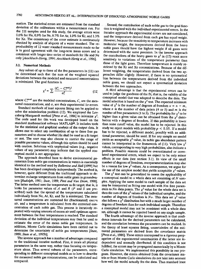
The synthetic data sets were used to explore same generalproperties of the problem. For example, consider a hypothet-ical groundwater sampIe that equilibrated at T = 10°C andP = 1 alm, has a contribution of excess air of A = 3 x 10 -3cm3 STP g-l (ANe = 27%), and S = R = 0 (Table 1). TheT -A model yields accurate results, with errors of 0.22°C für Tand 0.15 x 10-3 cm3 STP g-l tor A (Figure la). This resultwas cross-checked with Monte Carlo simulations by generatingrealizations of concentrations that were normally distributedaround the original values within the assigned error of 1 %. Foreach genera ted data set the optimal parameter values werecalculated, and their distribution was analyzed. Since the dis-tribution of the parameters is not necessarily normal, its me-dian and the width which contains 68.3% of the values werecalculated. For example, a Monte Carlo run with 1000 realiza-tions yielded approximately normal parameter distributionswith T = (10.007 :!: 0.216) °C andA = (2.995 :!: 0.147) x10 -3 cm3 STP g-l. With only 100 realizations, similar results

were obtained. Thus the Monte Carlo errors closely corre-spond to the errors calculated tram the covariance matrix, as

9 10 11

temperature rC]

Figure 1. Contours of the ~ surface in the parameter space,calculated tor the first synthetic data set of Table 1 with theWeiss solubilities. Contours tor ~ = 0.1, 0.5, 1, 2, and 4 areshown in both plots. (a) T -A model. T and A are not corre-lated, the ~ surface is nearly circular, and the minimum is weildefined. (b) T-P-A model, with a two-dimensional-section inthe T -P plain. Note the larger T scale compared to Figure la.T and P are correlated, and the ~ surface is strongly elliptical,which increases the parameter errors [see Press et al., 1986].

2784 AESCHBACH:HERnG ET AL.: INTERPRETAnON OF DISSOLVED ATMOSPHERIC NOBLE GASES

Table 2. Concentration Changes lnduced by SpecifiedSmall Changes of the Parameters Relative to the FirstData Set of Table 1

the parameters because the largest differences between thethree sets of solubilities are of the same magnitude as theexperimental uncertainties (1%). However, in contrast to ran-dom errors the switch of solubilities introduces systematicaldeviations.

ParameterChanges

.1He,%

~Ne,%

.lKr,%

.1Ac,%

~Xe,%

~T = 1°C~S=I%o~p = 0.01 almM = 10-4 cm3 STP g~R = 0.1

-0.32 -0.74 -2.12 -2.71 "'-3.35-0.42 -0.48 -0.67 -0.72 -0.77

0.76 0.80 0.94 0.98 0.990.84 0.71 0.23 0.12 0.06

-4.44 -2.03 -0.42 -0.14 -0.06

4.2. Air-Equilibrated WaterAs an overall test of the method including the experimental

and numerical methods as weil as the literature solubilities,sampies of air-equilibrated wateT at several different temper-atures were produced. Three large (-30 L) containers three-quarter filled with tap water and open to ambient air wereplaced in temperature stabilized rooms at temperatures ofabout 4°, 15°, and 30°C (sam pies CI-C3). A fourth containerwas placed in OUT noble gas laboratory, where the temperatureis relatively stahle near 20°C (sam pie LI). The wateT was verygently stirred to accelerate gas exchange while avoiding anyoccurrence of bubbles. The wateT was exposed tor approxi-mately 10 days, sincewe estimated"'that it may take several daysto reach complete equilibrium (height of the wateT columnabout 0.5 m and gas exchange velocities of the order of 1 md-l). Both wateT temperature and ambient atmospheric pres-sure were monitored over the entire period. Whereas temper-ature soon became stahle within the precision of measurement(::!:O.I°C), the pressures varied typically by a few mbar over thetime of exposure. The average pressure of the last 7 daysbefore sampling was used. A few measurements of electricalconductivity were made in order to estimate salinity (except torsampie LI). Sampies were drawn tram a bottom outlet of thecontainers with the usual techniques.

Surprisingly, it is not possible to fit all five noble gases withthe assumption of atmospheric equilibrium, because of an ex-cess of He. The Ne concentrations show that this excess cannotbe of atmospheric origin, except tor sampie LI. We suspectthat the He partial pressure in the air-conditioned rooms,located below ground level and vented only artificially, wasslightly enhanced relative to air, because of the presence ofradiogenic He. Indeed, the 3HetHe ratios of sampIes CI-C3are slightly below the atmospheric equilibrium value given byBenson and Krause [1980]. Thus, tor these sampies, He wasexcluded tram the fit tor T as the only free parameter. Sam pieLI can be fitted in the same way. However, only the T -A modelfils the measured concentrations of all five gases.l This inter-pretation of sampIe LI appears more likely and yields theheller agreement with the measured wateT temperature.

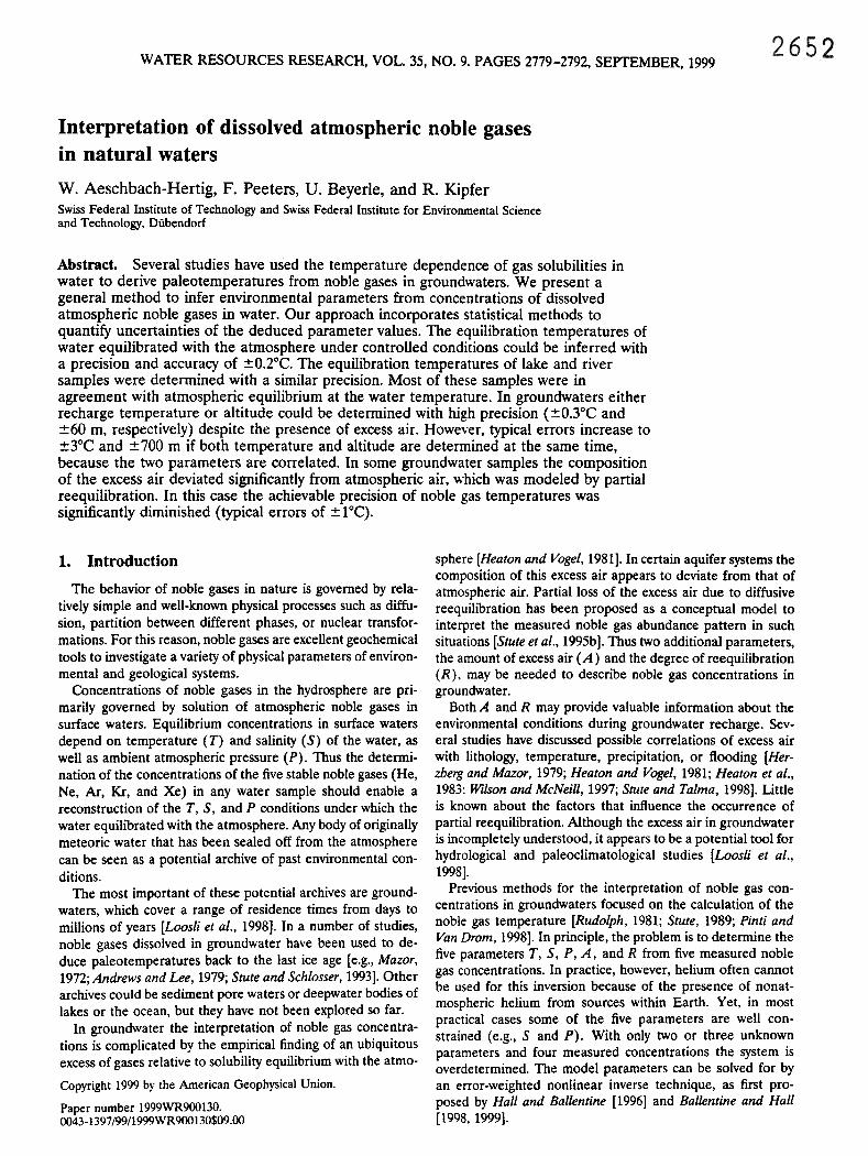
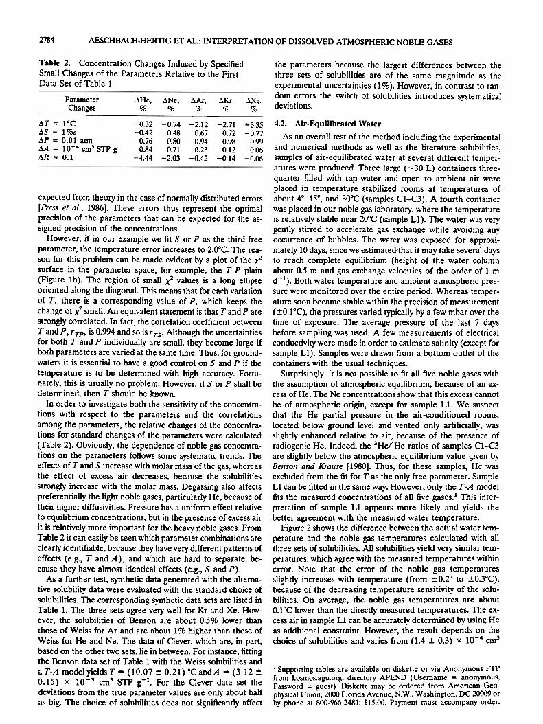
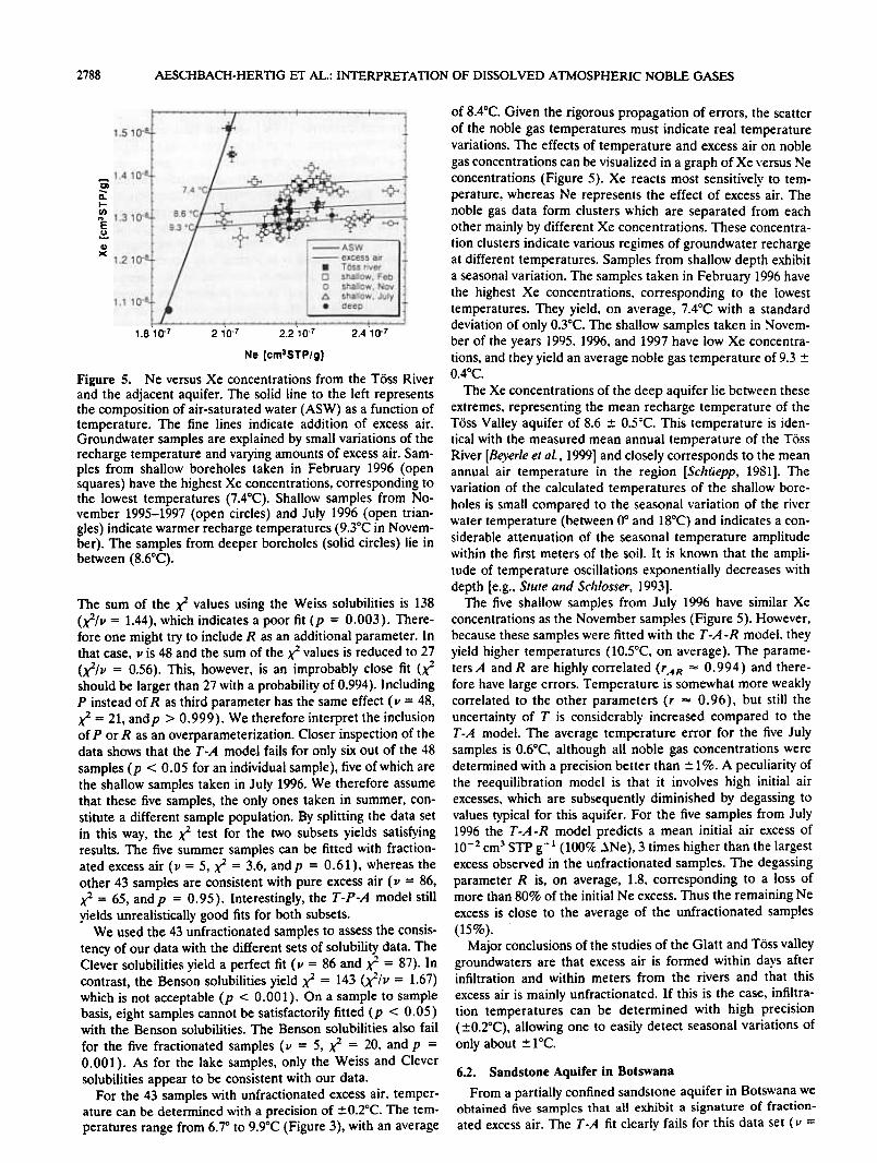
Figure 2 shows the difference between the actual wateT tem-perature and the noble gas temperatures calculated with allthree sets of solubilities. All solubilities yield very similar tem-peratures, which agree with the measured temperatures withinerror. Note that the error of the noble gas temperaturesslightly increases with temperature (from ::!:O.2° to ::!:O.3°C),because of the decreasing temperature sensitivity of the solu-bilities. On average, the noble gas temperatures are aboutO.I°C lower than the directly measured temperatures. The ex-cess air in sampIe LI can be accurately determined by using Heas additional constraint. However, the result depends on thechoice of solubilities and varies tram (1.4 ::!: 0.3) x 10-4 cm3

expected from theory in the case of normally distributed errors[Press er al., 1986]. These errors thus represent the optimalprecision of the parameters that can be expected tor the as-signed precision of the concentrations.

However, if in our example we fit S or P as the third freeparameter, the temperature error increases to 2.0°C. The rea-son tor this problem can be made evident by a plot of the x"surface in the parameter spate, tor example, the T -P plain(Figure Ib). The region of sm all x" values is a long ellipseoriented along the diagonal. This means that tor each variationof T, there is a corresponding value of P, which keeps thechange of x" smalI. An equivalent statement is that T and P arestrongly correlated. In fact, the correlation coefficient betweenT and P, r TP, is 0.994 and so is r TS. AIthough the uncertaintiestor both T and P individually are smalI, they become large ifboth parameters are varied at the same time. Thus, tor ground-waters it is essential to have a good control on Sand P if thetemperature is to be determined with high accuracy. Fortu-nately, this is usually no problem. However, if S or P shall bedetermined, then T should be known.

In order to investigate both the sensitivity of the concentra-tions with respect to the parameters and the correlationsamong the parameters, the relative changes of the concentra-tions tor standard changes of the parameters were calculated(Table 2). Obviously, the dependence of noble gas concentra-tions on the parameters follows some systematic trends. Theeffects of T and S increase with molar mass of the gas, whereasthe effect of excess air decreases, because the solubilitiesstrongly increase with the molar mass. Degassing also affectspreferentially the light noble gases, particularly He, because oftheir higher diffusivities. Pressure has a uniform effect relativeto equilibrium concentrations, but in the presence of excess airit is relatively more important tor the heavy noble gases. FromTable 2 it can easily be seen which parameter combinations areclearly identifiable, because they have very different patterns ofeffects (e.g., T andA), and which are hard to separate, be-cause they have almost identical effects (e.g., Sand P).

As a further test, synthetic data generated with the alterna-tive solubility data were evaluated with the standard choice ofsolubilities. The corresponding synthetic data sets are listed inTable 1. The three sets agree very weil tor Kr and Xe. How-ever, the solubilities of Benson are about 0.5% lower thanthose of Weiss tor Ar and are about 1% higher than those ofWeiss tor He and Ne. The data of Clever, which are, in part,based on the other two sets, lie in between. For instance, fittingthe Benson data set of Table 1 with the Weiss solubilities anda T-A modelyields T = (10.07:!: 0.21) °CandA = (3.12:!:0.15) x 10-3 cm3 STP g-l. For the Clever data set thedeviations from the true parameter values are only about halfas big. The choice of solubilities does not significantly affect

1 Supporting tables are available on diskette or via Anonymous FTPtram kosmos.agu.org, directory APEND (Usemame = anonymous,Password = guest). Diskette may be ordered trom American Geo-physical Union, 2000 Florida Avenue, N.W., Washington, DC 20009 orby phone at 800-966-2481; $15.00. Payment must accompany order.

AESCHBACH-HERnG ET AL.: INTERPRETAnON OF DISSOLVED ATMOSPHERIC NOBLE GASES 2785

STP g-l (Benson) to (2.3 :!: 0.3) x 10-4 cm3 STP g-l (Weiss).For the other three sampies the solubilities of Clever andBenson do not favor the presence of any excess air, whereasthe Weiss solubilities te nd toward positive values of excess air.In fact, the Weiss solubilities always yield the highest values fürexcess air, because they are about 1% lower than those ofBenson für He and Ne. Therefore care should be taken in theinterpretation of very small amounts of excess air, für example,in lakes or the ocean. Overall, the equilibrated sampies con-firm the consistency of the experimental and numerical meth-ods, although slight systematical deviations cannot be ex-cluded.

10 I I 1III 1 , -~

9.5~

~ 9fGI~ 8.5-'GI>.EI- ~

7

7~6.5~~-1~" 11 I I "-,

6.5 7 7.5 8 8.5 9 9.5 10

T iterative [.C]

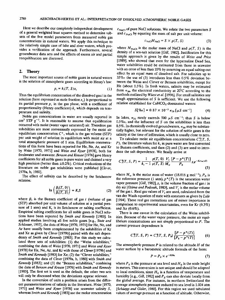
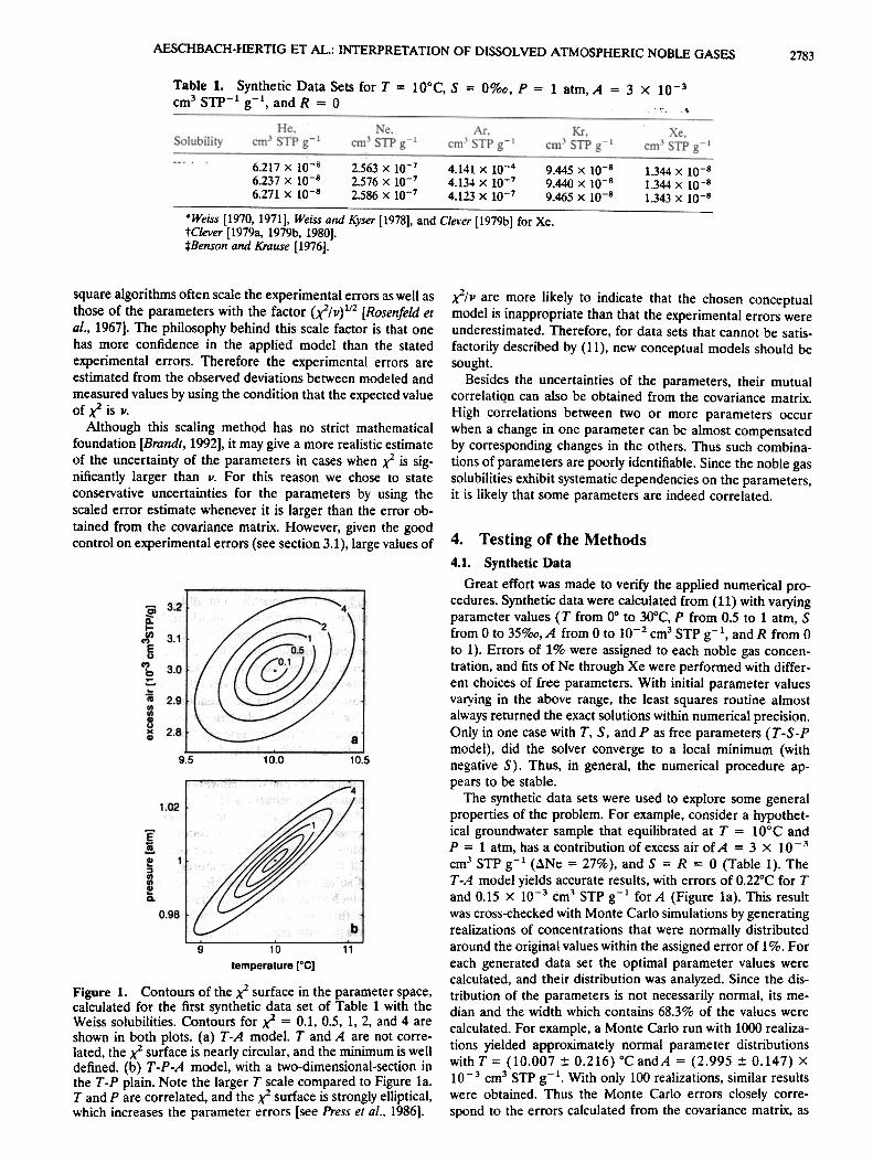
Figure 3. Comparison of noble gas temperatures calculatedwith the iterative method according to Sczlte [1989] and withOUT inverse procedure für 43 groundwater sampIes from theTöss Valley ~ith unfractionated excess air. Points show theresults obtained with the Weiss solubilities in the inverse cal-culations, which is the same database as used in the iterativemethod, except für Kr. Errors für the iterative technique wereestimated from the spread of the individual noble gas temper-atures. The lines represent linear regressions through the dataobtained with the three different sets of solubility data used inthe inverse calculations. The temperatures derived from thetwo methods closely agree, irrespective of the solubility data-base.

4.3. Comparison With the Iterative Technique

For comparison, 43 sam pies tram a shallow alluvial aquiferwhich contains unfractionated excess air (see section 6.1) wereevaluated with the iterative technique and solubilities as usedby Stute [1989], as weil as with OUT inverse procedure, using allthree sets of solubility data. The resulting noble gas tempera-tures of all sampies agree within erraT, independent of thechoice of solubility da ta (Figure 3). Furtherrnore, the errorsestimated tram the standard deviation of the individual noblegas temperatures in the iterative technique are, on average, ingood agreement with the rigorous erraT estimates obtained\\ith the error-weighted inverse method.

The noble gas temperatures calculated with OUT procedureand the Weiss solubilities are, on average, O.O7°C higher thanthose calculated with the iterative technique, although thesame solubilities were used except tor Kr. The deviation is aresult of the fact that tor this data set the Xe temperaturecalculated with the iterative approach is, on average, O.17°Chigher than the me an noble gas temperature. Because the Xeconcentration has the largest infiuence on the temperature inthe inverse approach, this small systematic bias leads to adifference between the two methods. However, this is a featureof this particular data set and does not indicate a generaloffset

between the two methods. The strength of the inverse ap-proach is not that it yields more accurate noble gas tempera-tures but that it allows one to estimate all parameters and thatit provides rigorous statistical tools.

0.2 I

O.ÜL

~GI..

I-.-

I. I.

--IC2

-

C1on..01

GI:c0c

C3.-0.2

1-0.3

.I- ~ wejSS 0 Clever

0 Benson

-0... , I I I I I ,0 5 10 15 20 25 30

T wale, [OC]

Figure 2. Oeviations of calculated noble gas temperaturestram directly measured water temperature of artificially equil-ibrated water sampies. Calculations were performed with thesolubilities of Weiss [1970, 1971] and Weiss and Kyser [1978],Clever [1979a, b, 1980], and Benson and Krause [1976]. The 10'errors are given tor the values calculated with the Weiss solu-bilities. Sampies CI-C3 were evaluated with T as the only freeparameter and without the He concentration. For sampie Ll,He was included and a T -A model was fitted.

5. Lake and River SampiesTo our knowledge, no measurements of all live noble gases

in lakes have been published, although a number of tritium-He-Ne studies have been performed in lakes [Torgersen et al.,1977; Kipfer er al., 1994; Aeschbach-Hertig et al., 1996]. Yetnoble gases are of use für the study of several processes inlakes. For instance, gas exchange and its dependency on dif-fusivity can be addressed [Torgersen et al., 1982]. Excess air maybe less important tor lakes than für the ocean, because break-ing waves are less frequent, hut this remains to be shown. Theimportance of bubble inclusion in rivers is even more uncer-tain. Excess air due to inftow of groundwater has been ob-served in same small alpine lakes [Aeschbach-Hertig, 1994].Thus the interaction of groundwater with civeTs or lakes couldpotentially be studied with noble gases. Furthermore, ques-tions related to the thermal structure of lakes and processes oftheir deepwater renewal may be addressed by noble gas mea-surements. Deepwater temperatures in so me lakes are signif-icantly affected by the geothermal heat ftux [e.g., Wüest et al.,1992], which should lead to a deviation between noble gas andin situ temperature.

In most cases. however, lake and river waters can be ex-pected to be or have been in close equilibrium with the atmo-sphere at their in situ temperature. Because all relevant pa-rameters für the calculation of equilibrium concentrations, thatis, temperature, salinity, and altitude, can be measured easilyand accurately in lakes, they provide a further test of the noble

2786 AESCHBACH-HERnG ET AL: INTERPRETAnON OF DISSOLVED ATMOSPHERIC NOBLE GASES

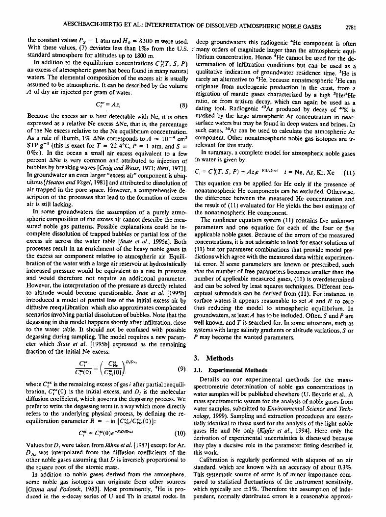
7 I r~:~Lake Baik~1 i/c Caspian Sea

R .glacier ponds

.rivers .~G>

~1;~0-E2!.

'"'"CIG>

:c0c

J:tf

~

~~j

:111

'-CL '" , , : i01234567

-~ -.+c-- ~

!

3./'-

ÜL 3.4GI

(3.2tE~111

~ 2.8-GI

:cg 2.6

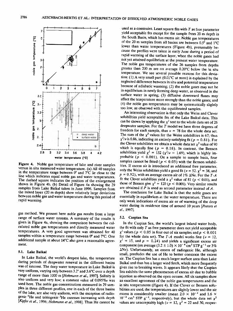
used as a constraint, Least square fits with Tas free parameteryield acceptable fits except tor the sampie tram 20 m depth inthe South Basin, which has excess air. Noble gas temperaturesof the 20 m sam pies tram all basins are between 0.5° and 1°Clower than wafer temperatures (Figure 4b), presumably be-cause the profiles were taken in early June during aperiod ofrapid warming of the surface layer, when the noble gases badnot yet attained equilibrium at the present water temperature.The noble gas temperatures of the 26 sam pies flom depthsgreater than 200 m are on average 0.20°C below the in situtemperature. We see several possible reasons für this devia-tion: (1) A very small part (O.OI°C at most) is explained by theneglected difference between in situ and potential temperaturebecause of adiabatic warming; (2) the noble gases may not bein equilibrium in newly forming deep wafer, as observed in thesurface wateT in spring; (3) diffusive downward fluxes mayaffect the temperature more strongly than the noble gases; and(4) the noble gas temperatures may be systematically slightlytao low, as observed withthe equilibrated sampies.

An interesting observation is that only the Weiss and Cleversolubilities yield acceptable fits of the Lake BaikaI data. Thiscan be shown by applying the ~ test to the whole data set of 26deepwater sampies. For the T model we have three degrees offreedom für each sampie, thus v = 78 für the whole data set.The sum of the ~ values für the Weiss solubilities is 67; thus~/v is 0.86, indicating an entirely satisfying fit (p = 0.81). Forthe Clever solubilities we obtain a whole data set ~ value of 90which is equally fine (p = 0.16). In contrast. the Bensonsolubilities yield ~ = 132 (~/v = 1.69), which is highly im-probable (p < 0.001). On a sampie to sampie basis, toursampies cannot be fitted (p < 0.05) with the Benson solubil-ities. If excess air is introduced as additional free parameter,only the Weiss solubilities yield a good fit (v = 52. ~ = 38, andp = 0.92), with an average excess air of I % ~Ne. For the T-Afit the Clever solubilities yield a ~ value of 81 (p < 0.01), andthose of Benson give ~ = 120 (p < 0.001). Very similar resultsare obtained if P is used as second parameter instead of A .

The conclusion für lake BaikaI is that the noble gases areessentially in equilibrium at the wafer temperature. There areonly weak indications of excess air or of warming of the deepwater du ring its residence time of around 10 years [Peeters etal., 1997].

0 deep water

.surface water

2.4t. -.I ~ I 'I I I b :i

2.8 3 3.2 3.4 3.6 3.8 4 4.2

water temperature ["CI

Figure 4. Noble gas temperature of lake and river sampIesversus in situ measured water temperature. (a) AJl40 sampiesin the temperature range between 00 and 7°C lie close to theline which indicates equal noble gas and water temperatures.The dashed square indicates the position of the enlargementsho\\n in Figure 4b. (b) Detail of Figure 4a showing the 29sampIes from Lake Baikai taken in June 1996. Sampies fromthe mixed layer (20 m depth) show relatively large deviationsbetween noble gas and water temperature during this period ofrapid warming.

gas method. We present hefe noble gas results tram a largerange of surface wateT systems. A summary of the results isgiven in Figure 4a, showing the comparison between the cal-culated noble gas temperatures and directly measured wateTtemperatures. A very good agreement was obtained tor 40sampIes within a temperature range between 0° and 7°C. Oneadditional sam pIe at about 14°C also gave a reasonable agree-ment.

5.2. Caspian Sea

In the Caspian Sea, the world's largest inland water body,the fit with only T as free parameter does not yield acceptableK values (p < 0.05 in tour out of six sampIes and p < 0.001tor the whole data set). The T -A model works fine (v = 12,K = 15, and p = 0.24) and yields a significant excess air

component (on average (3.2 :!: 1.0) X 10-4 cm3 STP g-l or 3%olNe). Unfortunately, an excess of radiogenic He, althoughsmalI, precludes the use of He to better constrain the excessair. The Caspian Sea has a much larger surface area than LakeBaikaI and thus has a larger wind fetch, which more frequentlygives rise to breaking waves. It appears likely that the CaspianSea exhibits the same phenomenon of excess air due to bubbleinjection as observed on the open oceans. All six sampIes showan excellent agreement of the noble gas temperatures and thein situ temperatures (Figure 4). If the Clever or Benson solu-bilities are used, the temperatures are slightly lower and the airexcess is considerably smaller (mean 2.0 X 10-4 and 1.6 X10-4 cm3 STP g-l, respectively), but the whole data set ~values are unacceptably high (v = 12, ~ = 22 and 30, respec-

5.1. Lake BaikaIIn Lake BaikaI, the world's deepest lake, the temperature

during periods of deepwater renewal in the different basinswas of interest. The deep water temperature in Lake BaikaI isvery uniform, varying only between 3.20 and 3.6°C over a depthrange of more than 1000 m [Hohmann er al., 1997]. Salinity isalso uniform and very low; a constant value of 0.095%0 wasused here. The noble gas concentrations measured in 29 sam-pIes in three different profiles, ODe in each of the three basinsof the lake, are also very uniform, wirb the exception of radio-genic 4He and tritiogenic 3He excesses increasing with depth[Kipfer er 01., 1996; Hohmann er al., 1998]. Thus He cannot be

AESCHBACH-HERTIG ET AL.: INTERPRETATION OF DISSOLVED ATMOSPHERIC NOBLE GASES2787

6. Groundwater SampiesStute and Schlosser [1993] showed that noble gases in

groundwater measure the mean annual ground temperature,which in most cases is closely related to the mean annual airtemperature. However, noble gases in groundwater may servealso other purposes than paleotemperature reconstruction. Inmountainous areas adetermination of the recharge altitudecould help to locate the origin of spring water or groundwater.Moreover, the excess air component in groundwaters maycarry information which is at present only poorly understood.The conditions and processes that lead to the formation ofexcess air need more study in order to learn how to model andinterpret this component. We present noble gas data from abroad spectrum of aquifers to illustrate the range of conditionsthat may be encountered.

tively, and p = 0.04 and 0.003, respectively). Thus the data

tram Lake Baikai and the Caspian Sea appear to justify the useof the Weiss solubilities as standard choice.

The Caspian Sea has a mean salinity of approximately12.5%0 [Peeters et al., 1999]. The good agreement of noble gasand in situ temperatures demonstrates the validity of our sa-linity parameterization (3), although the ion composition ofCaspian Sea water differs tram both ocean water and NaCIbrines. Vice versa, the salinity of Caspian Sea water can bedetermined tram the noble gas data with aprecision of about:!: 1 %c if temperature is prescribed. This precision, however, isnot sufficient to address questions related to the role of salinityin the physics of the Caspian Sea.

5.3. Ponds and Rivers

Two noble gas sampIes from small ponds that often form atthe ends of alpine glaciers were analyzed in connection withstudiesof glacial meltwater. The ponds were open to the at-mosphere, although some ice was floating in them. Thereforethey were expected to be in atmospheric equilibrium at atemperature close to the freezing point and an atmosphericpressure of about 0.72 alm (2700 m altitude). However, theconcentrations of Ne through Xe fit these assumptions ratherpoorly. Better filS are obtained if excess air is taken into ac-count. Excess air in glacial meltwaters may originate from airtrapped in the ice. Because there is no reason to expect radio-genic He in the meltwater ponds, He can be used to check thehypothesis of an excess air component, which fenders the re-sults conclusive. The model without excess air must be rejectedbecause of very high K va lues (32 and 62, respectively, v = 4,andp < 0.001). With excess air the model fits the data nicely(K of 2.5 and 3.7, respectively, and v = 3), the noble gas

temperatures are in reasonable agreement with the measuredtemperatures (Figure 4), and the excess air is 1.8 X 10-4 cm3STP g-l on average. By inclusion of He as fit constraint, theerrors of Aare reduced from ~ 1.0 X 10-4 cm3 STP g-l to~0.3 X 10-4 cm3 STP g-l.

In the course of studies of riverbank infiltration to thegroundwater, two small rivers were sampled für noble gases tocheck the assumption of atmospheric equilibrium. As with theglacial ponds, the equilibrium is expected to hold also tor He.Indeed, all three sampIes from the Töss river in northemSwitzerland can be fitted \\'ith a simple T model tor all fivenoble gases. The noble gas and measured river temperaturesagree within ~0.5°C (Figure 4). The three sampIes cover arange from 40 to 15°C. However, the equilibrium assumptionclearly does not hold tor the sampIe from a tributary of theBrenno River in southem Switzerland. There, a significant airexcess of (3.6 ~ 1.3) X 10-~ cm3 STP g-l results even withoutincluding He. The noble gas temperature agrees reasonablyweil with the measured value. Including He changes the resultstor both T and A very little hut drastically reduces the uncer-tainty of the excess air to ~0.4 X 10-4 cm3 STP g-l.

In summary, the possibility of small amounts of excess aircannot be excluded in ponds and rivers. He is of great value fürthe study of the excess air, because of its sensitivity to thisparameter. Unfortunately, the use of He as a purely atmo-spheric gas appears possible only in shallow surface water,whereas deep lakes often contain significant amounts of radio-genic 4He and tritiogenic 3He.

6.1. Alluvial Aquifers in Switzerland

aur first example is a shallow, unconfined alluvial aquifernear Glattfelden in northem Switzerland, red by infiltrationtram the Glatt River. Five sampies were taken from boreholesin the immediate vicinity of the river where according to in-vestigations with 222Rn [Hoehn and von Gunten, 1989] the ageof the groundwater is only a few days. aur 3H/3He datingconfirmed these very small ages. The sampies from Glattfeldenlie between typical surface and groundwater sampies, becausethey have both low excess air and radiogenic He. Their inter-pretation is not unique. If He is excluded, three of the fivesampies can be fitted with T as the only free parameter. Allsam pies are consistent with a T -A model, with A rangingbetween 0 and 8 x 10-4 cm3 STP g-'. If He is included, onlythe T -A model is applicable. The minimum value of A is thenconstrained to 2.5 x 10-4 cm3 STP g-'. Apparently. at this si tethe residence time of the groundwater is so short that theprocess of excess air formation can actually be observed. Itseems to take plac~ within days after infiltration. With allmodels the resulting temperatures are in close agreement withthe temperature of the groundwater measured during sam-pling, except for Olle sampie.

The second groundwater example is from a nearby and hy-drogeologically very similar site, where the Töss River feeds analluvial gravel and sand aquifer. Sampies were taken at differ-ent times of the year to investigate the influence of differentriver water levels on infiltration, mainly by means of 3H/3Hedating [Beyerle et al., 1999]. 3H/3He ages range between 0 and1 year tor most of the sampies from shallow bore holes andbetween 1 and 2 years für most of the deeper sampies. Noblegases of 48 sampies were analyzed to determine the rechargetemperature and to study the formation of excess air. In fact,although the river water is close to equilibrium (see section5.3), all groundwater sampies contain appreciable amounts ofexcess air, even those tram wells within meters of the riverbank and with vanishing 3H/3He ages within the error of atleast a month. Thus a T -A model was used to fit the data,yielding excess air arnounts from 3 X 10-4 to 3 X 10-3 cm3STP g-'. Although there is only little radiogenic excess He,inclusion of He as fit target is not possible tor most sampies.However, the results of the fits based on the other noble gasescan be used to determine the atmospheric 3He componentneeded tor the calculation of the 3H/3He ages.

It is useful to evaluate the K test for this whole data set of48 sampies. With the T -A model we have two degrees offreedom for each sampie thus v = 96 tor the whole data set.

2788 AESCHBACH-HERnG ET AL.: INTERPRETAnON OF DISSOLVED ATMOSPHERIC NOBLE GASES

'CiD:l-(/) ,

E~GI)(

'.8'0-7 2'0-7 2.2"0-7 2.4"0:7-

Ne [cm3STP/g]

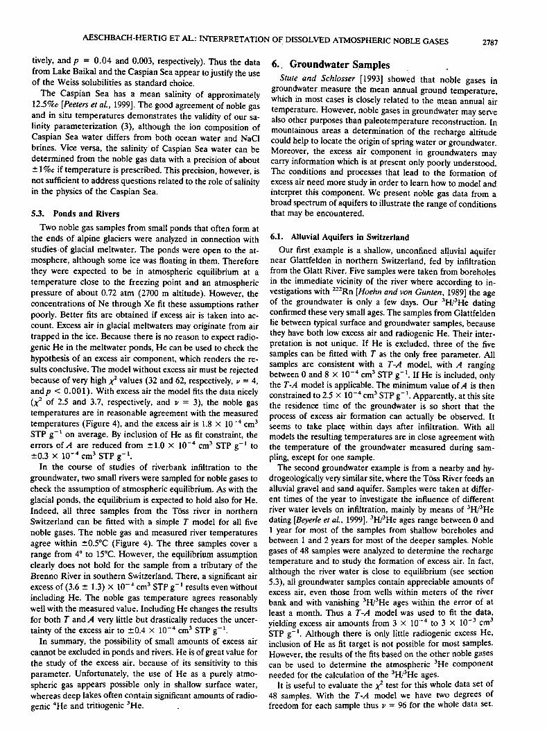
Figure 5. Ne versus Xe concentrations tram the Töss Riverand the adjacent aquifer. The solid line to the left representsthe composition of air-saturated water (ASW) as a function oftemperature. The fine lines indicate addition of excess air.Groundwater sampies are explained by sm all variations of therecharge temperature and varying amounts of excess air. Sam-pies from shallow bore holes taken in February 1996 (opensquares) have the highest Xe concentrations, corresponding tothe lowest temperatures (7.4°C). Shallow sampies tram No-vember 1995-1997 (open circles) and July 1996 (open trian-gles) indicate warmer rech arge temperatures (9.3°C in Novem-ber). The sampies from deeper boreholes (solid circles) lie inbetween (8.6°C).

The sum of the ~ values using the Weiss solubilities is 138(~/v = 1.44), which indicates a poor fit (p = 0.003). There-fore one might try to include R as an additional parameter. Inthat case, v is 48 and the sum of the ~ values is reduced to 27(~/v = 0.56). This, however, is an improbably dose fit (~should be larger than 27 wirb a probability of 0.994). IncludingP instead of R as third parameter has the same effect (v = 48,~ = 21, andp > 0.999). We therefore interpret the inclusionof P or R as an overparameterization. Closer inspection of thedata shows that the T -A model fails für only six out of the 48sampies (p < 0.05 für an individual sampie), five ofwhich arethe shallow sampies taken in July 1996. We therefore assumethat these five sampies, the only ones taken in summer, con-stitute a different sampIe population. By splitting the data setin this war, the ~ test für the two subsets yields satisfyingresults. The five summer sampies can be fitted with fraction-ated excess air (v = 5, ~ = 3.6, andp = 0.61), whereas theother 43 sampies are consistent with pure excess air (v = 86,~ = 65, andp = 0.95). Interestingly, the T-P-A model stillyields unrealistically good fits für both subsets.

We used the 43 unfractionated sampies to assess the consis-tency of OUT data with the different sets of solubility data. TheClever solubilities yield a perfect fit (v = 86 and ~ = 87). Incontrast, the Benson solubilities yield ~ = 143 (i/v = 1.67)

which is not acceptable (p < 0.001). On a sampie to sampiebasis, eight sampIes cannot be satisfactorily fitted (p < 0.05)with the Benson solubilities. The Benson solubilities also failfür the five fractionated sampies (v = 5, i = 20, and p =

0.001). As für the lake sampIes, only the Weiss and Cleversolubilities appear to be consistent with OUT data.

For the 43 sampies with unfractionated excess air, temper-ature can be determined with aprecision of :!:O.2°C. The tem-peratures range from 6. ~ to 9.9°C (Figure 3), with an average

of 8.4°C. Given the rigorous propagation of errors, the scatterof the noble gas temperatures must indicate real temperaturevariations. The effects of temperature and excess air on noblegas concentrations can be visualized in a graph of Xe \'ersus Neconcentrations (Figure 5). Xe reacts most sensitively to tem-perature, whereas Ne represents the effect of excess air. Thenoble gas data form clusters \\'hich are separated tram eachother mainly by different Xe concentrations. These concentra-tion clusters indicate various regimes of groundwater rech argeat different temperatures. SampIes tram shallow depth exhibita seasonal variation. The sam pies taken in February 1996 havethe highest Xe concentrations, corresponding to the lowesttemperatures. They yield. on average, 7.4°C with a standarddeviation of only 0.3°C. The shallow sampIes taken in Novem-ber of the years 1995. 1996, and 1997 have low Xe concentra-tions, and they yield an average noble gas temperature of 9.3 :!:0.4°C.

The Xe concentrations of the deep aquifer lie between theseextremes, representing the mean recharge temperature of theTöss Valley aquifer of 8.6 :!: 0.5°C. This temperature is iden-tical with the measured mean annual temperature of the TössRiver [Be)'erle et al., 1999] and closely corresponds to the meanannual air temperature in the region [Schüepp, 1981]. Thevariation of the calculated temperatures of the shallow bore-holes is small compared to the seasonal variation of the riverwafer temperature (between 0° and 18°C) and indicates a con-siderable attenuation of the seasonal temperature amplitudewithin the first meters of the soil. It is known that the ampli-tude of temperature oscillations exponentially decreases withdepth [e.g., Stute and Schlosser, 1993].

The five shallow sam pies from July 1996 have similar Xeconcentrations as the November sam pies (Figure 5). However.because these sampIes were fitted with the T -A -R model. theyyield higher temperatures (10.5°C, on average). The parame-tersA and Rare highly correlated (rAR = 0.994) and there-fore have large errors. Temperature is somewhat more weaklycorrelated to the other parameters (r = 0.96), hut still theuncertainty of T is considerably increased compared to theT -A model. The average temperature error tor the five Julysam pIes is 0.6°C, although all noble gas concentrations weredetermined with aprecision better than :!: 1 %. A peculiarity ofthe reequilibration model is that it involves high initial airexcesses, which are subsequently diminished by degassing tovalues typical tor this aquifer. For the five sam pies from July1996 the T -A-R model predicts a me an initial air excess of10-2 cm3 STP g-l (lOOCJc .1Ne), 3 times higher than the largestexcess observed in the unfractionated sampies. The degassingparameter R is, on average, 1.8. corresponding to a loss ofmore than 80% of the initial Ne excess. Thus the remaining Neexcess is close to the average of the unfractionated sampies

(15%).Major conclusions of the studies of the Glatt and Töss valley

groundwaters are that excess air is formed within days afterinfiltration and within meters tram the rivers and that thisexcess air is mainly unfractionated. If this is the case, infiltra-tion temperatures can be determined with high precision(:!:O,Z°C), allowing ODe to easily detect seasonal variations ofonly about :!: 1 °C.

6.2. Sandstone Aquifer in BotswanaFrom a partially confined sandstone aquifer in BotS\\'ana we

obtained five sam pIes that all exhibit a signature of fraction-ated excess air. Thc T -A fit clearly fails for this data set (11 =

AESCHBACH-HERTIG ET AL.: lr-.lERPRETATION OF DIS~OLYED ATMOSPHERIC NOBLE GASES2789

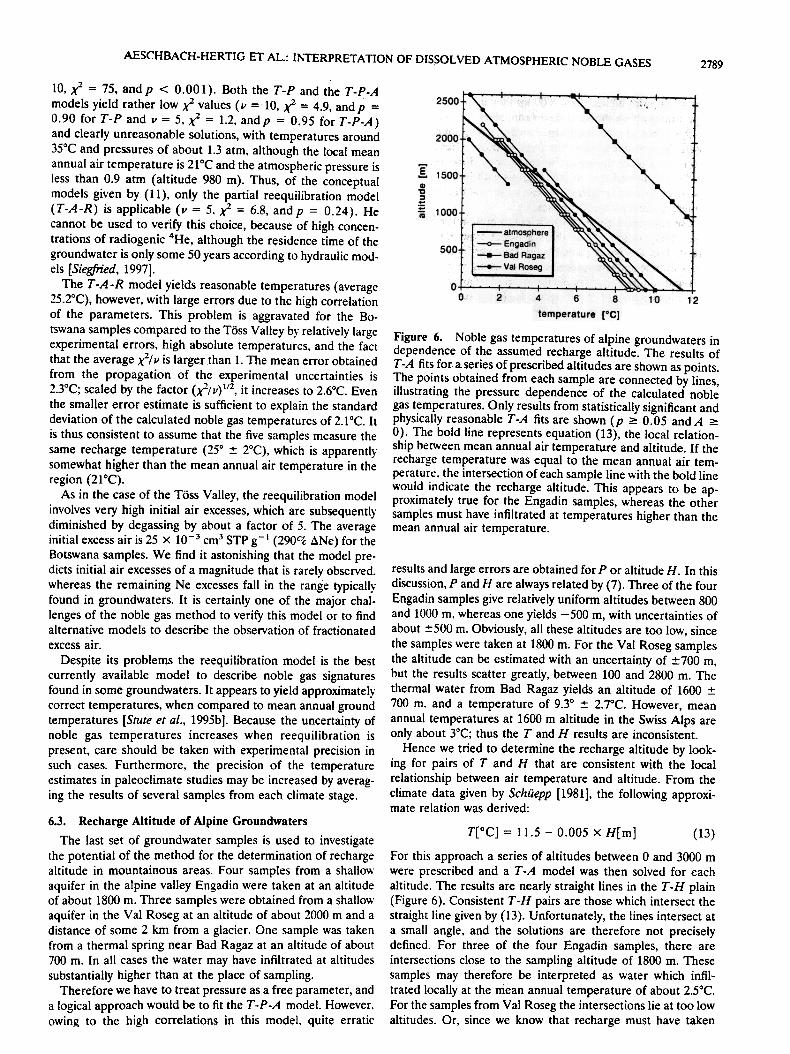
Figure 6. Noble gas temperatures of alpine groundwaters independence of the assumed recharge altitude. The results ofT -A fits für aseries of prescribed altitudes are shown as points.The points obtained from each sampIe are connected by lines,illustrating the pressure dependence of the calculated noblegas temperatures. Only results from statistically significant andphysicaIly reasonable T-A fits are shown (p ~ 0.05 andA ~0). The hold line represents equation (13), the local relation-ship berween mean annual air temperature and altitude. If therecharge temperature was equal to the me an annual air tem-perature. the intersection of each sampIe line with the hold linewould indicate the recharge altitude. This appears to be ap-proximately true für the Engadin sampIes, whereas the othersampIes must have infiltrated at temperatures higher than theme an annual air temperature.

results and large errors are obtained tor P or altitude H. In thisdiscussion, P and H are always related by (7). Tbree of the fourEngadin sam pIes give relatively uniform altitudes between 800and 1000 m, whereas one yields -500 m, with uncertainties ofabout :!:500 m. Obviously, all these altitudes are too low, sincethe sampIes were taken at 1800 m. For the Val Roseg sampIesthe altitude can be estimated with an uncertainty of :!:700 m,but the results scatter greatly, between 100 and 2800 m. Thethermal water from Bad Ragaz yields an altitude of 1600 :!:700 m. and a temperature of 9.3° :!: 2. rc. However, meanannual temperatures at 1600 m altitude in the Swiss Alps areonly about 3°C; thus the T and H results are inconsistent.

Hence we tried to determine the rech arge altitude by look-ing for pairs of T and H that are consistent with the localrelationship between air temperature and altitude. From theclimate data given by Schüepp [1981], the following approxi-mate relation was derived:

T[°C] = 11.5 -0.005 X H[m] (13)

For this approach aseries of altitudes between 0 and 3000 mwere prescribed and a T -A model was then solved für eachaltitude. Tbe results are nearly straight liDes in the T -H plaiD(Figure 6). Consistent T -H pairs are those which intersect thestraight line given by (13). Unfortunately, the lines intersect ata sm all angle, and the solutions are therefore not preciselydefined. For three of the four Engadin sampIes, there areintersections close to the sampling altitude of 1800 m. Thesesampies may therefore be interpreted as water which infil.trated locally at the mean annual temperature of about 2.5°C.For the sampies from Val Roseg the intersections lie at too lowaltitudes. Or, since we know that recharge must have taken

10, ~ = 75, and p < 0.001). Both the T -P and the T -P-Amodels yield rather low ~ values (v = 10, r = 4.9, and p =0.90 tor T-P and v = 5, ~ = 1.2, andp = 0.95 tor T-P-A)and clearly unreasonable solutions, with temperatures around35°C and pressures of about 1.3 atm, although the local meanannual air temperature is 21°C and the atmospheric pressure isless than 0.9 atm (altitude 980 m). Thus, of the conceptualmodels given by (11), only the partial reequilibration model(T-A-R) is applicable (v = 5; ~ = 6.8, andp = 0.24). Hecannot be used to veriiy this choice, because of high concen-trations of radiogenic 4He, although the residence time of thegroundwater is only some 50 years according to hydraulic mod-els [Siegfried, 1997].

The T -A-R model yields reasonable temperatures (average25.2°C), however, with large errors due to the high correlationof the parameters. This problem is aggravated tor the Bo-tswana sampIes compared to the Töss Valley by relatively largeexperimental errors, high absolute temperatures, and the factthat the average ~/v is largerthan 1. The me an error obtainedfrom the propagation of the experimental uncertainties is2.3°C; scaled by the factor (~/V)I/2, it increases to 2.6°C. Eventhe smaller error estimate is sufficient to explain the standarddeviation of the calculated noble gas temperatures of 2.1 °C. Itis thus consistent to assume that the five sampIes measure thesame recharge temperature (250 ::!: 2°C), which is apparentlysomewhat higher than the mean annual air temperature in the

region (21°C).As in the case of the Töss Valley, the reequilibration model

involves very high initial air excesses, which are subsequentlydiminished by degassing by about a factor of 5. The averageinitial excess air is 25 X 10-3 cm3 STP g-1 (290Cf ~Ne) tor theBotswana sampIes. We find it astonishing that the model pre.dicts initial air excesses of a magnitude that is rarely observed.whereas the remaining Ne excesses fall in the range typicallyfound in groundwaters. It is certainly one of the major chal-lenges of the noble gas method to veriiy this model or to findalternative models to describe the observation of fractionatedexcess air.

Despite its problems the reequilibration model is the bestcurrently available model to describe noble gas signaturesfound in some groundwaters. It appears to yield approximatelycorrect temperatures, when compared to mean annual groundtemperatures [Stute et al., 1995b]. Because the uncertainty ofnoble gas temperatures increases when reequilibration ispresent, care should be taken with experimental precision insuch cases. Furthermore, the precision of the temperatureestimates in paleoclimate studies may be increased by ave rag-ing the results of several sampIes from each climate stage.

6.3. Recharge Altitude of Alpine Groundwaters

The last set of groundwater samp.les is used to investigatethe potential of the method tor the determination of rech argealtitude in mountainous areas. Four sampIes from a shallo\\"aquifer in the alpine valley Engadin were taken at an altitudeof about 1800 m. Three sampies were obtained from a shallowaquifer in the Val Roseg at an altitude of about 2000 m and adistance of some 2 km from a glacier. One sam pIe was rakenfrom a thermal spring near Bad Ragaz at an attitude of about700 m. In all cases the wafer may have infiltrated at altitudessubstantially higher than at the place of sampling.

Therefore we have to treat pressure as a free parameter, anda logical approach would be to fit the T -P-A model. However,owing to the high correlations in this model. quite erratic

2790 AESCHBACH-HERTIG ET AL.: INTERPRETATION OF DISSOLVED ATMOSPHERIC NOBLE GASES

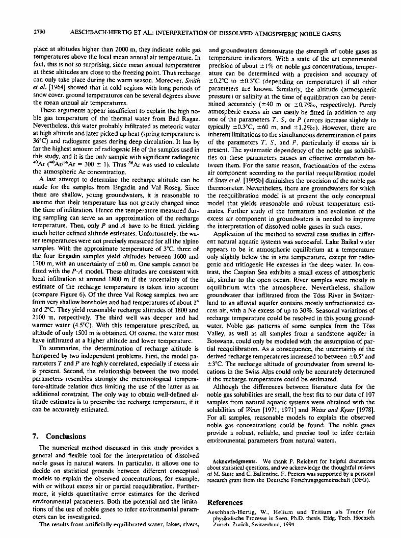
place at altitudes higher than 2000 m, they indicate noble gastemperatures above the Iocal mean annual air temperature. Infact, this is not so surprising, since mean annual temperaturesat these altitudes are close to the freezing point. Thus rech argecan only take place during the warm season. Moreover, Smithet al. [1964] showed that in cold regions with long periods ofsnow cover, ground temperatures can be several degrees abovethe mean annual air temperatures.

These arguments appear insufficient to explain the high no-ble gas temperature of the thermal water from Bad Ragaz.Nevertheless, this water probably infiltrated as meteoric wateTat high altitude and later picked up he at (spring temperature is36°C) and radiogenic gases during deep circulation. It has byfar the highest amount of radiogenic He of the sampIes used inthis study, and it is the only sampIe with significant radiogenic40 Ar (40 Ar/36 Ar = 300 ~ 1). Thus 36 Ar was used to calculate

the atmospheric Ar concentration.A last attempt to determine the recharge altitude can be

made für the sampies flom Engadin and Val Roseg. Sincethese are shallow, young groundwaters, it is reasonable toassume that their temperature has not greatly changed sincethe time of infiltration. Hence the temperature measured dur-ing sampling can serve as an approximation of the rechargetemperature. Then, only P and A have to be fitted, yieldingmuch better defined altitude estimates. UnfortunateIy, the wa-ter temperatures were not precisely measured für all the alpinesampIes. With the approximate temperature of 3°C, three ofthe tour Engadin sam pIes yield altitudes between 1600 and1700 m, with an uncertainty of ~60 m. Gne sampIe cannot befitted with the P-A model. These altitudes are consistent withlocal infiltration at around 1800 m if the uncertainty of theestimate of the rech arge temperature is taken into account(compare Figure 6). Gf the three Val Roseg sampIes, two arefrom very shallow bore holes and bad temperatures of about 1°and 2°C. They yield reasonable rech arge altitudes of 1800 and2100 m, respectively. The third weil was deeper and badwarmer water (4.5°C). With this temperature prescribed, analtitude of only 1500 m is obtained. Gf course. the water musthave infiltrated at a higher altitude and lower temperature.

To summarize, the determination of recharge altitude ishampered by two independent problems. First, the model pa-rameters T and P are highly correlated, especially if excess airis present. Second, the relationship between the two modelparameters resembles strongly the meteorological tempera-ture-altitude relation thus limiting the use of the latter as anadditional constraint. The only war to obtain well-defined al-titude estimates is to prescribe the recharge temperature, if itcan be accurately estimated.

and groundwaters demonstrate the strength of noble gases astemperature indicators. With astate of the art experimentalprecision of about :!:: 1 o/c on noble gas concentrations, temper-ature can be determined with aprecision and accuracy of:!::0.2°C to :!::0.3°C (depending on temperature) if all otherparameters are kno,vn. Similarly, the altitude (atmosphericpressure) or salinity at the time of equilibration can be deter-mined accurately (:!::40 m or ::0.7%0, respectively). Purelyatmospheric excess air can easily be fitted in addition to anyone of the parameters T. S, or P (errors increase slightly totypically =03°C, :!::60 m, and ::1.2%0). However, there areinherent limitations to the simultaneous determination of pairsof the parameters T, S, and P, particularly if excess air ispresent. The systematic dependency of the noble gas solubili-fies on these parameters causes an effective correlation be-tv.'een them. For the same reason, fractionation of the excessair component according to the partial reequilibration modelof Stute er al. [1995b] diminishes the precision of the noble gasthermometer. Nevertheless; there are groundwaters für whichthe reequilibration model is at present the only conceptualmodel that yields reasonable and robust temperature esti-mates. Further study of the formation and evolution of theexcess air component in groundwaters is needed to improvethe interpretation of dissolved noble gases in such cases.

Application of the method to several case studies in differ-ent natural aquatic systems was successful. Lake BaikaI ,vaterappears to be in atmospheric equilibrium at a temperatureonly slightly below the in situ temperature, except für radio-genic and tritiogenic He excesses in the deep wafer. In con-trast, the Caspian Sea exhibits a small excess of atmosphericair, similar to the open ocean. River sampies were mostly inequilibrium with the atmosphere. Nevertheless, shallowgroundwater that infiltrated tram the Töss River in Switzer-land to an alluvial aquifer contains mostly unfractionated ex-cess air, ,\"ith a Ne excess of up to 30%. Seasonal variations ofrech arge temperature could be resolved in this young ground-wateT. Noble gas patterns of some sampies from the TössValley, as weil as all sam pies tram a sandstone aquifer inBotswana. could only be modeled with the assumption of par-tial reequilibration. As a consequence, the uncertainty of thederived recharge temperatures increased to between :!::0.5° and::3°C. The recharge altitude of groundwater from severallo-cations in the Swiss Alps could only be accurately determinedif the recharge temperature could be estimated.

Although the differences between literature data für thenoble gas solubilities are small, the best fits to OUT data of 107sam pies from natural aquatic systems were obtained wirb thesolubilities of Weiss [1971, 1971] and Weiss and Kyser [1978].For all sampies, reasonable models to explain the observednoble gas concentrations could be found. The noble gasesprovide a robust, reliable, and precise tool to inter certainenvironmental parameters from natural wafers.

7. ConclusionsThe numerical method discussed in this srudy provides a

general and flexible tool für the interpretation of dissolvednoble gases in natural waters. In particular, it allows one todecide on statistical grounds between different conceptualmodels to explain the observed concentrations, für example,with or without excess air or partial reequilibration. Further-more, it yields quantitative error estimates für the derivedenvironmental parameters. Both the potential and the limita-tions of the use of noble gases to inter environmental param-eters can be investigated.

The results {rom artificially equilibrated water, lakes, rivers,

Ackno,,-Iedgments. We thank P. Reichert for helpful discussionsabout statistical quest ions, and we acknowledge the thoughtful re\1ewsof M. Stute and C. Ballentine. F. Peeters was supported by a personalresearch grant from the Deutsche Forschungsgemeinschaft (DFG).

ReferencesAeschbach-Hertig, W., Helium und Tritium als Tracer für

physikalische Prozesse in Seen, Ph.D. thesis. Eidg. Tech. Hochsch.Zurich. Zurich, Switzerland. 1994.

AESCHBACH-HERTIG ET AL.: INTERPRETATION OF DlSSOLVED ATMOSPHERIC NOBLE GASES2791

Aeschbach-Hertig, W., R. Kipfer, M. Hofer, D. M. Imboden, andH. Baur, Density-driven exchange between the basins of Lake Lu-terne (Switzerland) traced with the 3H-3He method, Limnol. Ocean.ogr., 41. 707-721,1996.

Andrews. J. N., and D. J. Lee. Inert gases in groundwater from theBunter Sandstone of England as indicators of age and palaeocli-matic trends,J. HydroI., 41,233-252,1979.

Ballentine. C. J., and C. M. Hall, A non-linear inverse technique forcalculating paleotemperature and other variables using noble gasconcentrations in groundwater: The Last Glacial Maximum in thecontinental tropics re-examined (abstract), Min. Mag., 62A. 100-101, 1998.

Ballentine. C. J., and C. M. Hall, Determining paleotemperature andother variables using an error weighted non-linear inversion of noblegas concentrations in wafer, Geochim. Cosmochim. Acta, in press,1999.

Benson. B. B., and D. Krause, Empirical laws for dilute aqueoussolutions of nonpolar gases, J. Chem. Phys., 64, 689-709, 1976.

Benson. B. B., and D. Krause. Isotopic fractionation of helium duringsolution: A probe für the liquid grate, J. Solution Chem., 9, 895-909.1980.

Beyerle. U., W. Aeschbach-Hertig, M. Hofer. R. Kipfer, D. M. Imbo-den, and H. Baur, Infiltration of river wafer to a shallow aquiferinvestigated with 3H/3He, noble gases and CFCs,J. HydroI., in press,1999.

Bieri, R. H.. Dissolved noble gases in marine waters, Eal1h Planet. Sci.Lett.. 10, 329-333, 1971.

Brandt, S.. Datenanalyse: Mit statistischen Methoden und Computelpro.grammen, 3rd ed., 651 pp.. BI Wissenschaftsverlag. Mannheim. Ger-many. 1992.

Clever. H. L. (Ed.), Helium and Neon-Gas Solubilities, Int. Union PureAppl. Chem. Solubility Data Ser., val. 1, 393 pp., Pergamon. Tarry-town, N. Y., 1979a.

Clever, H. L. (Ed.), Krypton, Xenon and Radon-Gas Solubilities, Int.Union PI/re Appl. Chem. Solubility Data Ser., vol. 2, 357 pp.. Perga.mon, Tarrytown, N. Y., 1979b.

Clever, H. L. (Ed.), Argon, Int. Union Pure Appl. Chem. Solubili,!' DataSer., val. 4, 331 pp., Pergamon, Tarrytown, N. Y., 1980.

Craig, H.. and R. F. Weiss, Dissolved gas saturation anomalies andexcess helium in the ocean, Eal1h Planet. Sci. Lett., 10, 289-296,1971.

Gill, A. E., Atmosphere-Ocean Dynamics, 662 pp., Academic, San Di-ego, Calif., 1982.

Hall, C. M., and C. J. Ballentine, A rigorous mathematical method forcalculating paleotemperature, excess air, and paleo-salini~. fromnoble gas concentrations in groundwater (abstract), Eos Trans.AGU, 77, Fall Meet. Suppl., F178. 1996.

Heaton, T. H. E., and J. C. Vogel, "Excess air" in ground\\.ater, J.HydroI.. 50, 201-216. 1981.

Heaton, T. H. E., A. S. Talma, and J. C. Vogel, Origin and history ofnitrate in confined groundwater in the western Kalahari, J. H:vdrol.,62, 243-262, 1983.

Herzberg. 0., and E. Mazor, Hydrological applications of noble gasesand temperature measurements in underground water systems: Ex-amples from Israel, J. HydroI.. 41,217-231,1979.

Hoehn, E.. and H. R. von Gunten, Radon in groundwater: A tool toassess infiltration from surface waters to aquifers, Water Resour.Res., 25. 1795-1803, 1989.

Hohmann. R., R. Kipfer, F. Peeters, G. Piepke. D. M. Imboden, andM. N. Shimaraev, Processes of deep water renewal in Lake BaikaI.Limnol. Oceanogr., 42, 841-855, 1997.

Hohmann. R., M. Hofer, R. Kipfer, F. Peeters, and D. M. Imboden.Distribution of helium and tritium in Lake BaikaI. J. Geoph.\'s. Res..103, 12.823-12,838, 1998.

Jähne, B.. G. Heinz, and W. Dietrich, Measurement of the diffusioncoefficients of sparingly soluble gases in water, J. Geophys. Res.. 92,10,767-10,776. 1987.

Kipfer, R.. W. Aeschbach-Hertig, H. Baur, M. Hofer, D. M. Imboden,and P. Signer, Injection of mantle type helium info Lake Van (Tur-key): The clue for quantifying deep water renewal. Eal1h Planet. Sci.Lett., 125, 357-370, 1994.

Kipfer, R.. W. Aeschbach-Hertig, M. Hofer, R. Hohmann, D. M.Imboden, H. Baur, V. Golubev, and J. Klerkx, Bottomwater forma-tion due to hydrothermal activity in Frolikha Bay, Lake BaikaI.eastern Siberia, Geochim. Cosmochim. Acta, 60. 961-971, 1996.

Lide, D. R. (Ed.), CRC Handbook o[ Chemistry and Physics, 75th ed.,; 'CRC Press, Boca Raton, FIa., 1994.

Loosli. H. H., B. Lehmann, W. Aeschbach-Hertig, R. Kipfer, W. M.Edmunds, L. Eichinger, K. Rozanski, M. Stute, and R. Vaikmäe,Tools used to study paleoclimate help in water management, Eos,79, 576, 582, 1998.

Mazor. E., Paleotemperatures and other hydrological parameters de-duced from gases dissolved in groundwaters, Jordan Rift Valley,Israel. Geochem. Cosmochim. Acta, 36, 1321-1336, 1972.

Ozima. M., and F. A. Podosek, Noble Gas Geochemistry, 367 pp.,Cambridge Univ. Press, New York, 1983.

Peeters. F., R. Kipfer, R. Hohmann, M. Hofer, D. M. Imboden, G. G.Kodenev, and T. Khozder, Modelling transport rates in Lake Baikai:Gas exchange and deep water renewal, Environ. Sci. Technoi., 31,2973-2982, 1997.

Peeters. F., R. Kipfer, D. Achermann, M. Hofer, W. Aeschbach-Hertig, U. Beyerle, D. M. 1mboden, K. Rozanski, and K. Fröhlich,Analysis of deep-water exchange in the Caspian Sea based on envi-ronmental tracers, Deep Sea Res., Part I. in press, 1999.

Pinti, D. L., and E. Van Drom, PALEOTEMP: A MATHEMATICAprogram für evaluating paleotemperatures from the concentrationof atmosphere-derived noble gases in ground water, Comput.Geosci., 24, 33-41, 1998.

Press, W. H., P. F. Flannery, S. A. Teukolsky, and W. T. Vetterling,Numerical Recipes, 818 pp., Cambridge Univ. Press, New York, 1986.

Rosenfeld, A. H.. A. Barbaro-Galtieri, W. J. Podolsky, L. R. Price, P.Soding. C. G. Wohl, M. Roos, and W. J. Willis, Data on particles andresonant states. ReIo'. Mod. Phys., 39, I-51, 1967.

Rudolph. J., Edelgastemperaturen und Heliumalter 14C-datierterPaläowässer, Ph.D. thesis, Univ. of Heidelberg, Heidelberg, Ger-many. 1981.

Schüepp. M., Klima und Wetter, in Atlas der Schweiz, edited byE. Spiess, p. 11, Verlag der Eidg. Landestopogr., Wabern-Bern.Switzerland, 1981.

Schüepp. M., and O. Gisler, Luftdruck, in Beihefte zu den Annalen derSch.."eiz, Meteorol. Anst.. 23, Schweiz. Meteorol. Anst., Zurich, 1980.

Siegfried. T., Modeling of groundwater withdrawal and its conse-quences to the aquifer: A case study in semi-arid Botswana, Pal1aRoad area, Diploma thesis, Eidg. Tech. Hochsch. Zurich, Zurich,Switzerland, 1997.

Smith, G. D., F. Newhall, L. H. Robinson, and D. Swanson, Soiltempcrature regimes: Their characteristics and predictability, Rep.SCS-TP-I44, Soil Conserv. Serv., U.S. Dep. of Agric., Washington,D. C.. 1964.

Smith, S. P., and B. M. Kennedy, Solubility ofnoble gases in water andin NaO brine, Geochim. Cosmochim. Acta, 47, 503-515,1983.

Stute, t-,L, Edelgase im Grundwasser-Bestimmung von Paläotempera-turen und Untersuchung der Dynamik von Grundwasserfließsyste-men. Ph.D. thesis, Univ. ofHeidelberg, Heidelberg, Germany, 1989.

Stute, ~L, and P. Schlosser, Principles and applications of the noble gaspaleothermometer, in Climate Change in Continental IsotopicRecords, Geophys. Monogr. Ser., vol. 78, edited by P. K. Swart et al.,pp. 89-100, AGU, Washington, D. C., 1993.

Stute, t-,L. and A. S. Talma, Glacial temperatures and moisture trans-port rcgimes reconstructed from noble gases and 6180, Stamprietaquifer, Namibia, in Isotope Techniques in the Study o[ Environmen-tal Change, pp. 307-318, Int. Atom. Energy Agency, Vienna. 1998.

Stute, ~L. J. F. Clark, P. Schlosser, and W. S. Broecker, A 30.000 yrcontinental paleotemperature record derived from noble gases dis-solved in groundwater from the San Juan Basin, New Mexico, Quat.Res., -13, 209-220, 1995a.

Stute, ~., M. Forster, H. Frischkorn, A. Serejo, J. F. Clark,P. Schlosser, W. S. Broecker, and G. Bonani, Cooling of tropicalBrazil (5°C) du ring the Last Glacial Maximum, Science, 269, 379-383. 1995b.

Torgersen, T., Z. Top, W. B. Clarke, W. J. Jenkins, and W. S. Bro-ecker. A new method tor physicallimnology-tritium-helium-3 ag-es-Results für Lakes Erie, Huron and Ontario, Limnol. Oceanogr.,22, 181-193, 1977.

Torgerscn, T., G. Mathieu, R. H. Hesslein, and W. S. Broecker, Gasexchange dependency on diffusion coefficient: Direct 112Rn and "Hecomparisons in a smalllake, J. Geophys. Res., 87, 546-556, 1982.

Weiss, R. F., The solubility of nitrogen, oxygen and argon in water andseawater, Deep Sea Res. Oceanogr. Abstr., 17, 721-735, 1970.

Weiss, R. F., Solubility of helium and neon in water and seawater,J. Chem. Eng. Data, 16, 235-241, 1971.