Embed Size (px)
Citation preview
The Pennsylvania State University
The Graduate School
Department of Energy and Mineral Engineering
INTERPRETATION OF HYDRAULIC FRACTURING PRESSURE IN LOW-
PERMEABILITY GAS RESERVOIRS
A Thesis in
Energy and Mineral Engineering
by
Gun-Ho Kim
2010 Gun-Ho Kim
Submitted in Partial Fulfillment
of the Requirements
for the Degree of
Master of Science
December 2010

ii
The thesis of Gun-Ho Kim was reviewed and approved* by the following:
John Yilin Wang Assistant Professor of Petroleum and Natural Gas Engineering Thesis Advisor
Turgay Ertekin Professor of Petroleum and Natural Gas Engineering George E. Trimble Chair in Earth and Mineral Sciences Undergraduate Program Officer of Petroleum and Mineral Gas Engineering
Robert Watson Associate Professor Emeritus of Petroleum and Natural Gas Engineering and Geo-Environmental Engineering
*Signatures are on file in the Graduate School
iii
ABSTRACT
Hydraulic fracturing has been used in most oil and gas wells to increase production by
creating fractures that extend from the wellbore into the formation. There are many types of
pressure change during the fracturing process. However, it is very difficult to estimate those
pressure changes and to predict how a fracture propagates.
In the 1980s, Nolte and Smith initiated a model for interpreting hydraulic fracturing
pressures in conventional reservoirs and it still remains qualitative. An accurate interpretation of
hydraulic fracturing pressures, during injection and after shut-in, is critical to understand and
improve the fracture treatment in low-permeability gas formations such as tight sand and gas
shale. It would also provide additional information about the wellbore and better understanding of
the reservoir.
In this study, new models for the accurate calculation of bottomhole treating pressure
based on surface treating pressure were first developed. This calculation was determined by
incorporating hydraulic pressure, fluid friction pressure, fracture fluid property changes along the
wellbore, proppant effect, perforation effect, tortuosity, thermal effect, effect of casing, rock
toughness, in-situ stress. New methods were then developed for more accurate interpretation of
the net pressure and fracture propagation. The models and results were finally validated with field
data from tight gas and shale gas reservoirs.
iv
TABLE OF CONTENTS
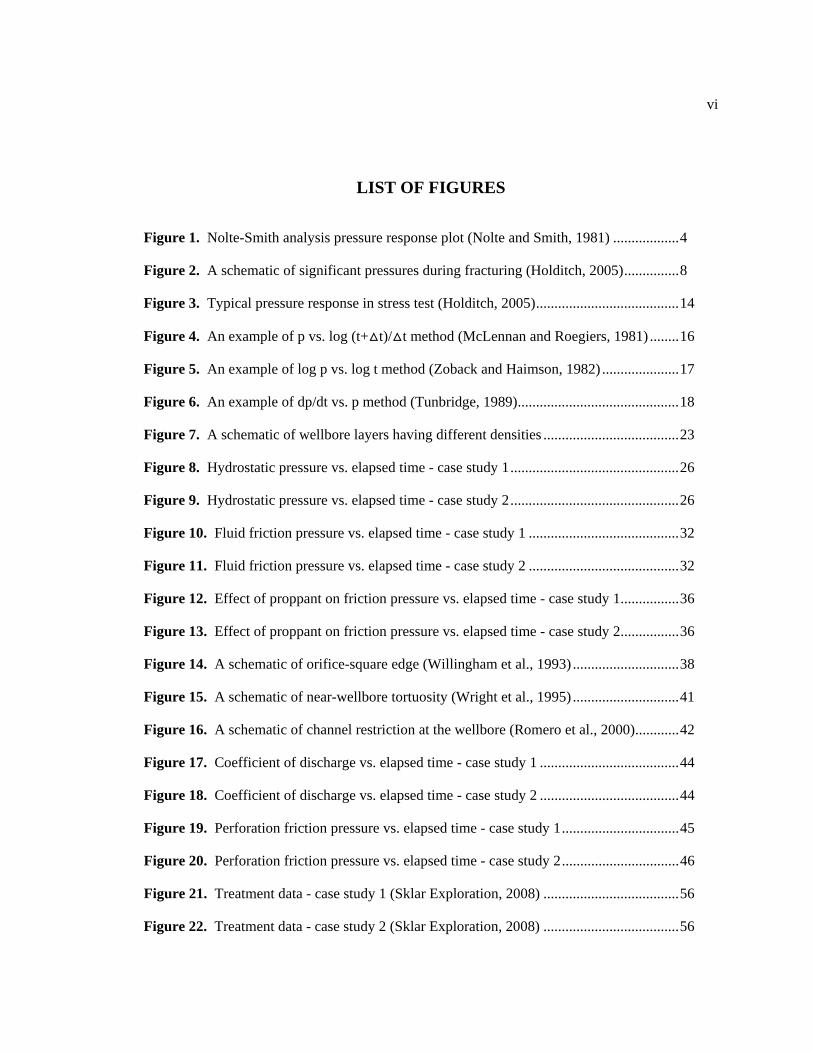
LIST OF FIGURES ................................................................................................................. vi
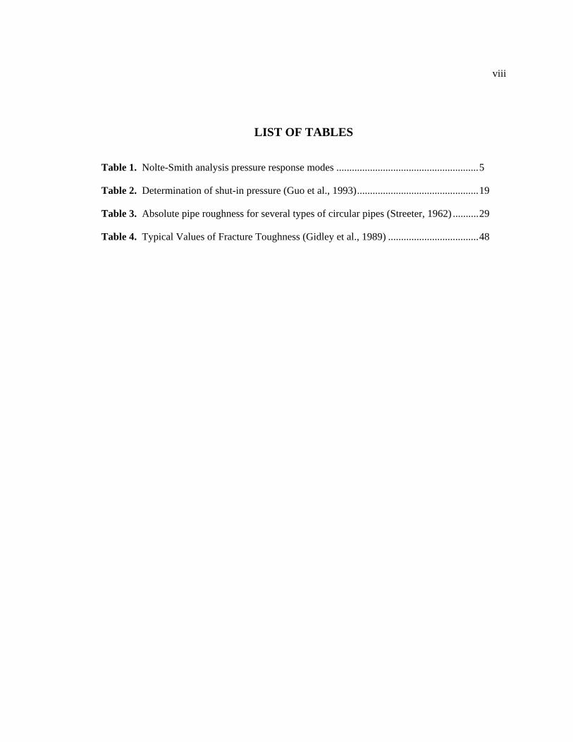
LIST OF TABLES ................................................................................................................... viii
ACKNOWLEDGEMENTS ..................................................................................................... ix
Chapter 1 INTRODUCTION ................................................................................................... 1
Chapter 2 LITERATURE REVIEW ........................................................................................ 3
2.1 Low-Permeable Gas Reservoirs ................................................................................. 3
2.2 Nolte and Smith Analysis .......................................................................................... 4
2.3 Different Types of Pressure ....................................................................................... 8
2.4 Predicting Pressure Loss due to Fluid Friction in the Wellbore................................. 12
2.5 Identifying In-Situ Stress by Instantaneous Shut-In Pressure (ISIP) ......................... 14
Chapter 3 STATEMENT OF THE PROBLEM ...................................................................... 20
Chapter 4 MODEL DEVELOPMENT AND VALIDATIONS ............................................... 22
4.1 Fracture Fluid Density Change along the Wellbore ................................................... 22 4.1.1 Equivalent Static Density and Equivalent Circulating Density ....................... 22 4.1.2 Applications to Field Data ............................................................................... 25 4.1.3 Results and Validations ................................................................................... 25
4.2 Effect of Casing Roughness ....................................................................................... 28 4.2.1 Fanning Friction Factor ................................................................................... 28 4.2.2 Applications to Field Data ............................................................................... 31 4.2.3 Results and Validations ................................................................................... 31
4.3 Effect of Proppant on Fluid Friction .......................................................................... 33 4.3.1 Proposed Method ............................................................................................. 33 4.3.2 Applications to Field Data ............................................................................... 35 4.3.3 Results and Validations ................................................................................... 35
4.4 Effect of Near-Wellbore Friction ............................................................................... 37 4.4.1 Perforation Pressure Loss ................................................................................ 37 4.4.2 Fracture Tortuosity Pressure ........................................................................... 41 4.4.3 Applications to Field Data ............................................................................... 43 4.4.4 Results and Validations ................................................................................... 43
4.5 Effect of Rock Toughness .......................................................................................... 47 4.5.1 Stress Intensity Factor ..................................................................................... 47 4.5.2 Applications to Field Data ............................................................................... 49 4.5.3 Results and Validations ................................................................................... 49
v
4.6 Thermal Effect on In-Situ Stress ................................................................................ 50 4.6.1 Thermal Expansion Stress ............................................................................... 50 4.6.2 Applications to Field Data ............................................................................... 51 4.6.3 Results and Validations ................................................................................... 51
4.7 Effect of Pore Pressure ............................................................................................... 52 4.7.1 Pore Pressure Expansion Stress ....................................................................... 52 4.7.2 Applications to Field Data ............................................................................... 53 4.7.3 Results and Validations ................................................................................... 53
Chapter 5 RESULTS AND ANALYSES ................................................................................ 55
5.1 Interpretation Pressures without Considering All Factors ......................................... 55 5.1.1 Calculation of Bottomhole Treating Pressure ................................................. 55 5.1.2 Identification of In-Situ Stress ........................................................................ 57 5.1.3 Interpretation of Fracture Propagation ............................................................ 60
5.2 Interpretation of Pressures with New Models ............................................................ 63 5.2.1 Changes in Hydrostatic Pressure ..................................................................... 63 5.2.2 Changes in Fluid Friction Pressure ................................................................. 64 5.2.3 Changes in Perforation Friction Pressure ........................................................ 64 5.2.4 Changes in In-Situ Stress ................................................................................ 65 5.2.5 Interpretation of Fracture Propagation ............................................................ 65
5.3 New Methods for Interpreting Fracture Geometry .................................................... 68 5.3.1 Fast Fourier Transform (FFT) and Deconvolution Method ............................ 68 5.3.2 Application to Field Data ................................................................................ 70 5.3.3 Interpretation of Fracture Propagation ............................................................ 71
Chapter 6 CONCLUSIONS AND RECOMMENDATIONS .................................................. 74
NOMENCLATURE ................................................................................................................ 76
REFERENCES ........................................................................................................................ 79
APPENDIX A - SUMMARY OF FRICTIONAL PRESSURE LOSS EQUATIONS ............ 83
APPENDIX B - CHARTS OF FRICTION FACTOR VS REYNOLDS NUMBER .............. 85
APPENDIX C - NET PRESSURE CALCULATION WITH FFT .......................................... 86
vi
LIST OF FIGURES
Figure 1. Nolte-Smith analysis pressure response plot (Nolte and Smith, 1981) .................. 4
Figure 2. A schematic of significant pressures during fracturing (Holditch, 2005) ............... 8
Figure 3. Typical pressure response in stress test (Holditch, 2005) ....................................... 14
Figure 4. An example of p vs. log (t+△t)/△t method (McLennan and Roegiers, 1981) ........ 16
Figure 5. An example of log p vs. log t method (Zoback and Haimson, 1982) ..................... 17
Figure 6. An example of dp/dt vs. p method (Tunbridge, 1989) ............................................ 18
Figure 7. A schematic of wellbore layers having different densities ..................................... 23
Figure 8. Hydrostatic pressure vs. elapsed time - case study 1 .............................................. 26
Figure 9. Hydrostatic pressure vs. elapsed time - case study 2 .............................................. 26
Figure 10. Fluid friction pressure vs. elapsed time - case study 1 ......................................... 32
Figure 11. Fluid friction pressure vs. elapsed time - case study 2 ......................................... 32
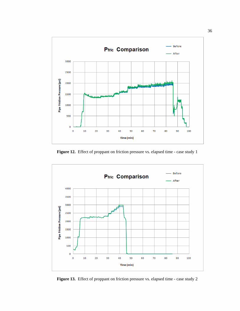
Figure 12. Effect of proppant on friction pressure vs. elapsed time - case study 1 ................ 36
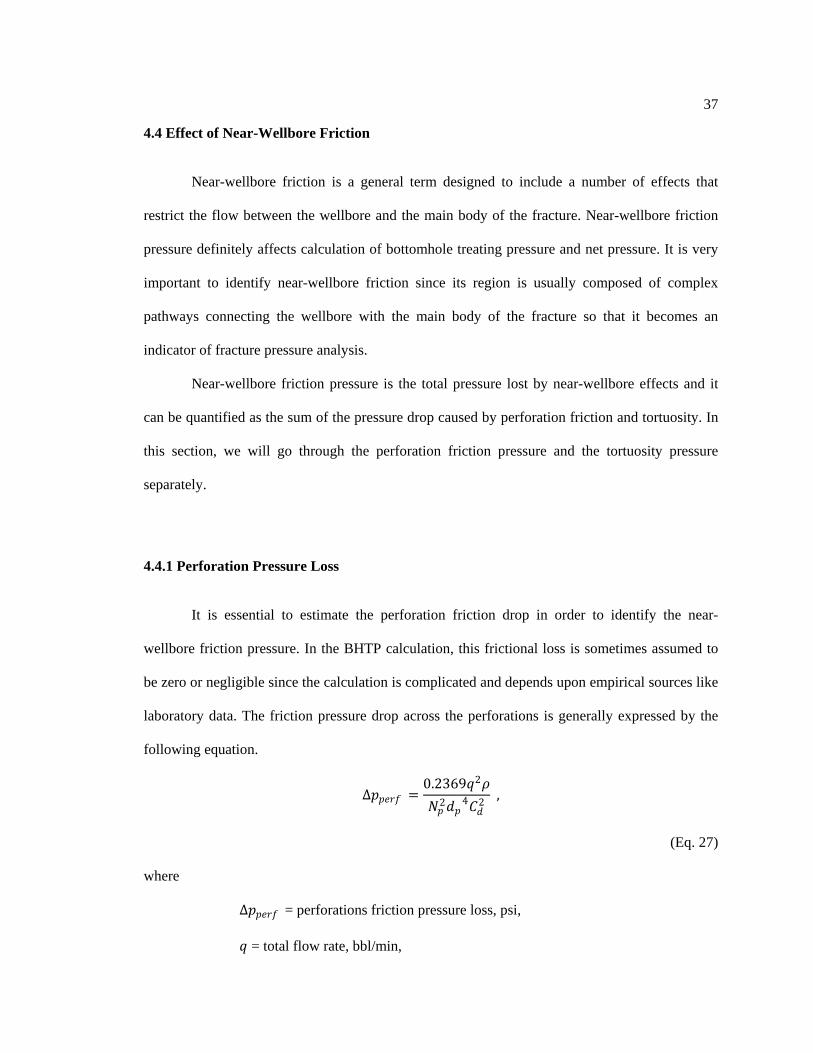
Figure 13. Effect of proppant on friction pressure vs. elapsed time - case study 2 ................ 36
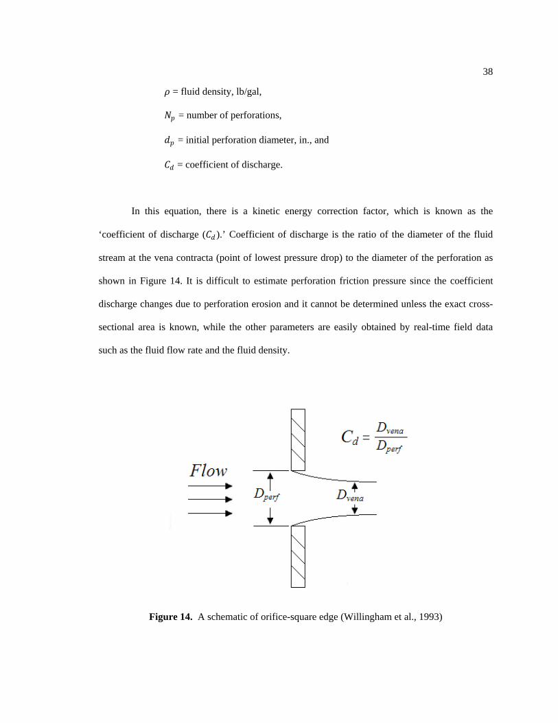
Figure 14. A schematic of orifice-square edge (Willingham et al., 1993) ............................. 38
Figure 15. A schematic of near-wellbore tortuosity (Wright et al., 1995) ............................. 41
Figure 16. A schematic of channel restriction at the wellbore (Romero et al., 2000) ............ 42
Figure 17. Coefficient of discharge vs. elapsed time - case study 1 ...................................... 44
Figure 18. Coefficient of discharge vs. elapsed time - case study 2 ...................................... 44
Figure 19. Perforation friction pressure vs. elapsed time - case study 1 ................................ 45
Figure 20. Perforation friction pressure vs. elapsed time - case study 2 ................................ 46
Figure 21. Treatment data - case study 1 (Sklar Exploration, 2008) ..................................... 56
Figure 22. Treatment data - case study 2 (Sklar Exploration, 2008) ..................................... 56

vii
Figure 23. Area where indistinct shut-in pressure appears - case study 1 .............................. 57
Figure 24. p vs. log (t+△t)/△t method application- case study 1 ........................................... 58
Figure 25. dp/dt vs. p method application- case study 1 ........................................................ 59
Figure 26. Net pressure plot without considering factors - case study 1 ................................ 60
Figure 27. Net pressure plot without considering factors - case study 2 ................................ 61
Figure 28. Net pressure plot after considering factors - case study 1 .................................... 66
Figure 29. Net pressure plot after considering factors - case study 2 .................................... 67
Figure 30. Net pressure when using a constant injection rate - case study 1 ......................... 71
Figure 31. Net pressure when using a constant injection rate - case study 2 ......................... 72
viii
LIST OF TABLES
Table 1. Nolte-Smith analysis pressure response modes ....................................................... 5
Table 2. Determination of shut-in pressure (Guo et al., 1993) ............................................... 19
Table 3. Absolute pipe roughness for several types of circular pipes (Streeter, 1962) .......... 29
Table 4. Typical Values of Fracture Toughness (Gidley et al., 1989) ................................... 48
ix
ACKNOWLEDGEMENTS
Before anything else, I want to say I love my parents and my brother who have always
trusted me no matter what I do. My family has been my spiritual support and the reason why I am
going for my goal.
I would first like to thank my thesis advisor, Dr. John Yilin Wang for his guidance,
patience, and confidence. Without his great help, this research would not have been possible.
I am greatly indebted to Dr. Turgay Ertekin who helped me make up my mind to keep
studying here at Penn State while I was thinking of transferring to other schools. As a matter of
fact, he introduced me to my advisor so that I have been able to enjoy studying petroleum
engineering. I would also like to thank Dr. Robert Watson for being on my thesis committee.
I also extend many thanks to every member in the Penn State 3S Laboratory who gave
me encouragement when I had a hard time doing my research. There are still many people that I
would like to thank, but I especially want to take the opportunity to thank Dennis Arun Alexis,
Hemant Kumar, Kyung-soo Kim, and Joseph Casamassima for their sincere advice.
1
Chapter 1
INTRODUCTION
Hydraulic fracturing has been one of the most effective techniques to increase the
productivity of wells by creating a conductive flow path. The significance of interpreting
hydraulic fracturing pressures has been recognized ever since this technique was first applied in
the 1950s.
Models have been developed to interpret hydraulic fracturing pressures and to evaluate
fracture propagation. The first attempt of interpretation of the geometry during a hydraulic
fracturing treatment was started by radial model, in which fracture width is proportional to
fracture radius. Another approach was developed as KGD (Khristianovich-Geertsma-de Klerk-
Daneshy) and PKN (Perkins-Kern-Nordgren) models. KGD model specifies that fracture height is
fixed and width is proportional to fracture length, assuming constant width against height and
slippage at the formation boundaries. In PKN model, the fracture height is also assumed to be
constant. However, there is no slippage between the formation boundaries, and the width is
proportional to fracture height.
A method for interpreting fracturing pressure response was created by Nolte and Smith in
the early 1980s. On the basis of PKN, KGD, and radial models, Nolte and Smith analyzed the
pressure response and predicted certain types of behavior based on the response. The Nolte-Smith
analysis has played a significant role in evaluating fracture treatments in oil and gas wells
worldwide. It provides a quick look and preliminary evaluation of the fracture treatment.
However, this method remains qualitative because of the assumptions in the Nolte-Smith method
and difficulties in the accurate calculation of net pressure. The assumptions include constant
2
injection rate, constant fluid viscosity, fractures in the vertical plane, and no slip of boundaries
along the horizontal planes that confine the fracture height. Factors affecting net pressure
calculation include fracture fluid property changes along the wellbore, effect of casing roughness,
proppant effect on fluid friction, effects of perforation friction drop, tortuosity effect, effect of
rock toughness, and thermal and pore pressure effects on in-situ stress.
In this research, I will develop new models for accurate calculation of net pressure by
considering all the pertinent factors. Then I will develop a new method to eliminate the
assumptions that the Nolte-Smith method made. These will lead to an accurate interpretation of
fracture propagation.
3
Chapter 2
LITERATURE REVIEW
2.1 Low-Permeable Gas Reservoirs
Production from low-permeability formations has become a major source of natural gas
supply. In 2008, low-permeability reservoirs accounted for about 40 percent of natural gas
production and about 35 percent of natural gas consumption in the United States. Low-
permeability gas formations include the shale, sandstone, carbonate, and coal bed whose matrix
permeability is 0.1 mD or less (EIA, 2010).
The use of hydraulic fracturing in tight sand and the use of hydraulic fracturing in
conjunction with horizontal drilling in shale gas formations have unlocked natural gas resources
that were not economical before. As shale gas production has expanded into more basins and the
technology has improved, the amount of shale gas reserves has increased dramatically. However,
the understanding of the fracture propagation in these low-permeability formations is still limited.
New knowledge in this area should increase the reserve and improve the recovery.
4
2.2 Nolte and Smith Analysis
The Nolte-Smith analysis was introduced in 1981 and it has been used to interpret net
pressure when 2-D models were broadly used for fracture design and most fractures were
vertically contained during fracture propagation. Based on PKN fracture geometry (Perkins and
Kern, 1972), KGD (Khristianovich and Geertsma and de-Klerk, 1969) and radial models, Nolte
and Smith analyzed the fracturing pressure response, and then predicted fracture behaviors based
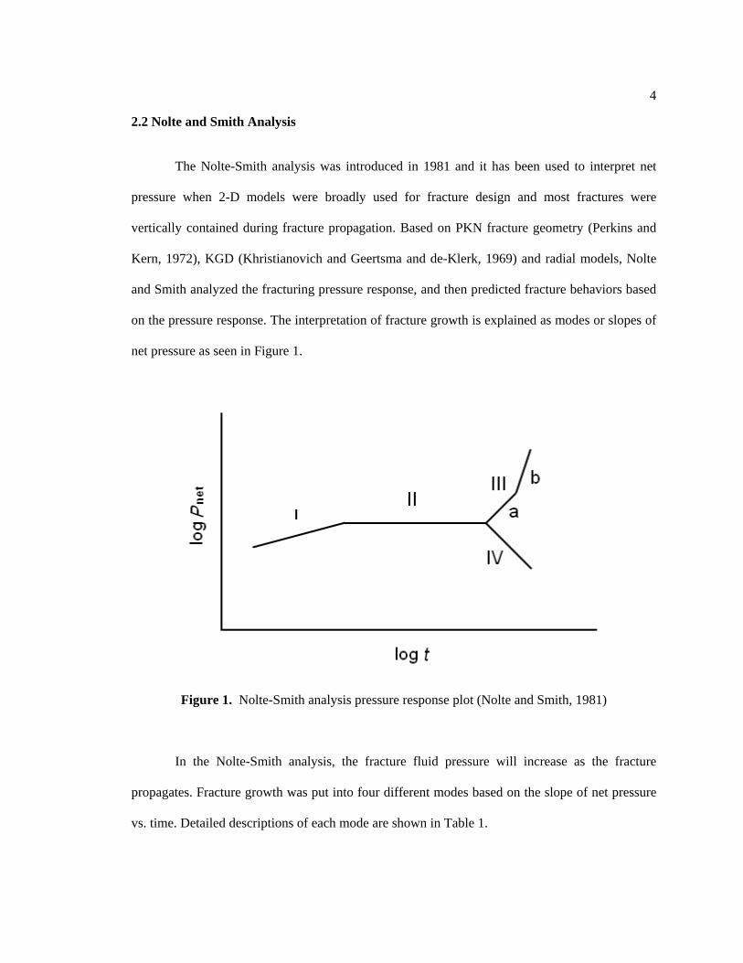
on the pressure response. The interpretation of fracture growth is explained as modes or slopes of
net pressure as seen in Figure 1.
Figure 1. Nolte-Smith analysis pressure response plot (Nolte and Smith, 1981)
In the Nolte-Smith analysis, the fracture fluid pressure will increase as the fracture
propagates. Fracture growth was put into four different modes based on the slope of net pressure
vs. time. Detailed descriptions of each mode are shown in Table 1.
5
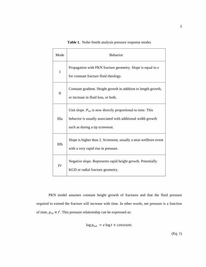
Table 1. Nolte-Smith analysis pressure response modes
Mode Behavior
I Propagation with PKN fracture geometry. Slope is equal to e
for constant fracture fluid rheology.
II Constant gradient. Height growth in addition to length growth,
or increase in fluid loss, or both.
IIIa
Unit slope. Pnet is now directly proportional to time. This
behavior is usually associated with additional width growth
such as during a tip screenout.
IIIb Slope is higher than 2. Screenout, usually a near-wellbore event
with a very rapid rise in pressure.
IV Negative slope. Represents rapid height growth. Potentially
KGD or radial fracture geometry.
PKN model assumes constant height growth of fractures and that the fluid pressure
required to extend the fracture will increase with time. In other words, net pressure is a function
of time, pnet ∝ te. This pressure relationship can be expressed as:
log 𝑝𝑝𝑛𝑛𝑛𝑛𝑛𝑛 = 𝑛𝑛 log 𝑛𝑛 + 𝑐𝑐𝑐𝑐𝑛𝑛𝑐𝑐𝑛𝑛𝑐𝑐𝑛𝑛𝑛𝑛.
(Eq. 1)
6
This means that fractures displaying PKN fracture geometry would have a straight line
with a slope of e on a plot of log pnet against log t. This stands for Mode I on the Nolte-Smith plot
in Figure 1. In power law fluid systems, the time exponent, e, is defined with upper and lower
boundaries as:
�1
4𝑛𝑛′ + 4� < 𝑛𝑛 < �
12𝑛𝑛′ + 3
� .
(Eq. 2)
These upper and lower boundaries are the outcome of solving a polynomial equation.
This means that for practical values of n’, the lower boundary of e will be between 0.25 and
0.125, while the upper boundary will be from 0.333 to 0.2. Those values are obtained when we
put n’=0 and n’=1 into Eq. 2. So any straight line on a Nolte-Smith plot with a gradient between
0.333 and 0.125 possibly indicates very good height containment. For Newtonian fluids (n’=1),
the range of the exponent becomes 0.125< e <0.2.
Small Positive Slope (Mode I)
As a result, the initial portion of the curve in Figure 1, denoted as Mode I, indicates
confined height, constant compliance, and unrestricted extension of fracture length. The
interpretation could be made that the fracture is propagating normally.
Constant Pressure (Mode II)
This portion of the curve is the most difficult to provide a definitive physical description.
However, this portion is potentially the most important. According to the Nolte-Smith analysis,
this mode indicates larger increase in fluid loss, height, or compliance than with respect to the

7
desired small positive slope mode. In general, the constant pressure region preceded an
undesirable height growth or rapid increases in pressure.
Unit Slope (Mode III)
A unit log-log plot, denoted as Mode IIIa, implies that the pressure is proportional to time
or, more significantly, the incremental injected-fluid volume. It also implies that an obvious flow
restriction has occurred in the fracture like proppant screenout. The difference between Modes
IIIa and IIIb is determined by the distance from the wellbore. If the distance is large, a screenout
probably occurs near the tip and can be used to estimate the propped penetration. But if the
distance is small, the screenout likely occurs near the wellbore with abnormal fluid loss.
Negative Slope (Mode IV)
The negative slope is interpreted as rapid height growth. The basic premise of this area is
that any significant decrease in fracture pressure probably results from unstable height growth. A
significant increase in fluid loss is possible but is not likely with decreasing pressure. Thus, the
most probable cause of a significant pressure decrease must be a significant increase in height
(Nolte and Smith, 1981).
8
2.3 Different Types of Pressure
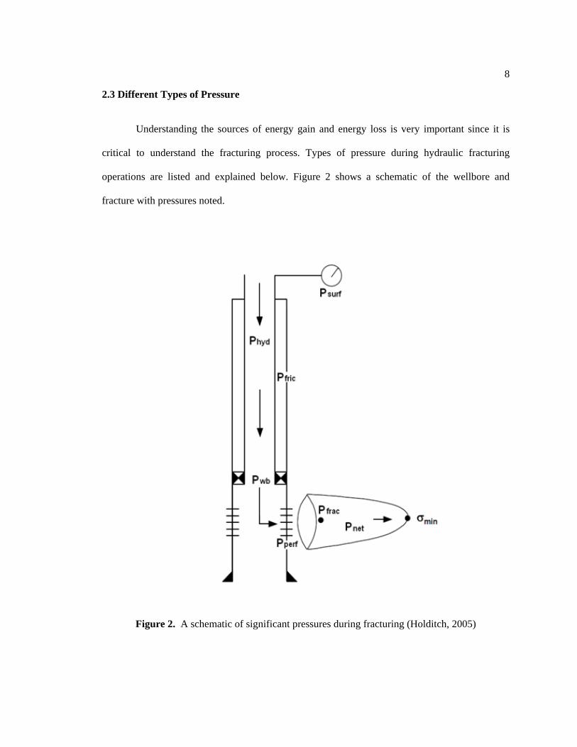
Understanding the sources of energy gain and energy loss is very important since it is
critical to understand the fracturing process. Types of pressure during hydraulic fracturing
operations are listed and explained below. Figure 2 shows a schematic of the wellbore and
fracture with pressures noted.
Figure 2. A schematic of significant pressures during fracturing (Holditch, 2005)

9
Surface Treating Pressure (STP), psurf
This is also known as wellhead pressure or injection pressure. It is the pressure measured
by the gauge at the wellhead where the fracture fluids are pumped through.
Hydrostatic Pressure, phyd
This pressure is the hydrostatic pressure exerted by the fracture fluid due to its depth and
its density changes. In petroleum engineering fields, it is used as:
𝑝𝑝ℎ𝑦𝑦𝑦𝑦 = 0.0052 ∗ 𝜌𝜌 ∗ ℎ ,
(Eq. 3)
where ρ is the slurry density (lb/gal) and h is the total vertical depth (ft).
Fluid Friction Pressure, pfric
This is also referred to as tubing friction pressure or wellbore friction pressure. It is the
pressure loss due to friction effect in the wellbore as fluids are injected.
Bottomhole Treating Pressure (BHTP), pwb
This pressure is also referred to as wellbore pressure. It is the downhole pressure, in the
wellbore, in the center of the interval being treated. BHTP can be calculated from surface data as
follows:
𝑝𝑝𝑤𝑤𝑤𝑤 = 𝑝𝑝𝑐𝑐𝑠𝑠𝑠𝑠𝑠𝑠 + 𝑝𝑝ℎ𝑦𝑦𝑦𝑦 − 𝑝𝑝𝑠𝑠𝑠𝑠𝑓𝑓𝑐𝑐 .
(Eq. 4)
10
Perforation friction Pressure, △pperf
This is the pressure lost as the fracturing fluid passes through the restricted flow area of
the perforations. Perforation friction pressure can be calculated by:
△ 𝑝𝑝𝑝𝑝𝑛𝑛𝑠𝑠𝑠𝑠 = 0.2369 ∗𝑞𝑞2𝜌𝜌
𝑁𝑁𝑝𝑝2𝐷𝐷𝑝𝑝4𝐶𝐶𝑦𝑦2 ,
(Eq. 5)
where ρ is the slurry density (lb/gal), q is the total flow rate (bpm), Np is the number of
perforations and Dp is the perforation’s diameter (inches) and Cd is the discharge coefficient.
Tortuosity Pressure, ptort
This is known simply as tortuosity. This pressure is the pressure loss as fracture fluid
passes through a region of restricted flow between the perforation and the main body of the
fracture.
Fracturing Fluid Pressure, pfrac
This pressure is the pressure of the fracturing fluid inside the main body of the fracture,
after it has passed through the perforations and any tortuous path. Fracturing fluid pressure may
not be constant over the entire fracture due to friction effect inside the fracture. It is calculated as
follows:
𝑝𝑝𝑠𝑠𝑠𝑠𝑐𝑐𝑐𝑐 = 𝑝𝑝𝑤𝑤𝑤𝑤 −△ 𝑝𝑝𝑝𝑝𝑛𝑛𝑠𝑠𝑠𝑠 .
(Eq. 6)
11
In-Situ Stress, σ1
This is also referred to as closure pressure or minimum horizontal principal stress. It is
the stress within the formation, which acts as a load on the formation. It is also the minimum
stress required inside the fracture in order to keep it open. For a single layer, it is usually equal to
the minimum horizontal stress, allowing for the effect of pore pressure. Otherwise, it is the
average stress over all the layers.
Net Pressure, pnet
This is the excess pressure in the fracturing fluid inside the fracture, above that required
to simply keep the fracture open. Net pressure can be calculated as follows:
𝑝𝑝𝑛𝑛𝑛𝑛𝑛𝑛 = 𝑝𝑝𝑠𝑠𝑠𝑠𝑐𝑐𝑐𝑐 − 𝜎𝜎1 .
(Eq. 7)
The importance of the net pressure cannot be overemphasized during fracturing. The net
pressure, multiplied by the fracture volume, provides us with the total quantity of energy
available at any given time to make the fracture grow. How that energy is used (generation of
width, splitting of rock, fluid loss or friction loss) is determined by the fracture model being
employed to simulate fracture growth.
12
2.4 Predicting Pressure Loss due to Fluid Friction in the Wellbore
One of the fundamental objects of fluid mechanics, as far as the fracturing engineer is
concerned, is to predict the friction pressure of fluids that are being injected. This is not easy
because fluid composition and temperature is continually changing during the treatment process.
Furthermore, friction reducers decrease friction coefficients so that the friction pressure
decreases. Normally, we predict friction pressure by using friction pressure tables and using data
provided by the actual treatment process. Most modern fracture simulators incorporate field data
in their fluid models, so friction pressures estimated by these are also rationally reliable if there is
no proppant in the fluid.
Reynold’s Number
The friction pressure depends on the flow regime. Thus, it is significant to determine the
flow regime. This is found by using the Reynold’s number, as follows:
Plug Flow NRe < 100
Laminar Flow 100 < NRe < 2000
Turbulent Flow NRe > 2000.
and the Reynold’s number for pipe flow can be found using:
𝑁𝑁𝑅𝑅𝑛𝑛 = 132,624 ∗𝜌𝜌𝑞𝑞𝑦𝑦𝑑𝑑
,
(Eq. 8)
where 𝜌𝜌fluid is the fluid density in lb/gal, q is the flow rate in bpm, d is the inside diameter in
inches, and μ is the fluid viscosity in cp. However, Eq. 8 only applies to Newtonian fluids, i.e.,
fluids with a constant viscosity. In the fracturing field, engineers mostly deal with complex fluids,
so below is the equation converted for power law fluids:
13
𝑁𝑁𝑅𝑅𝑛𝑛 = 1.86 ∗𝜌𝜌𝜌𝜌2−𝑛𝑛′
𝐾𝐾′ �96𝑦𝑦 �
𝑛𝑛′ ,
(Eq. 9)
where υ is the velocity in ft/sec, n’ is the power law exponent, and K’ is the power law
consistency index (Appendix A). To make things easier, 𝜌𝜌 can be easily found from the flow rate:
𝜌𝜌 = 17.157 ∗𝑄𝑄𝑦𝑦2 .
(Eq. 10)
Fluid Friction Pressure
Fanning’s method uses a friction factor determined by using the Reynold’s number. For
plug and laminar flow:
𝑠𝑠 =16𝑁𝑁𝑅𝑅𝑛𝑛
,
(Eq. 11)
and for turbulent flow for smooth pipes:
𝑠𝑠 ≈0.0303𝑁𝑁𝑅𝑅𝑛𝑛1.1612 .
(Eq. 12)
Therefore, the fluid friction pressure would be calculated as:
𝑝𝑝𝑠𝑠𝑠𝑠𝑓𝑓𝑐𝑐 = 0.039 ∗𝐿𝐿𝜌𝜌𝜌𝜌2𝑠𝑠𝑦𝑦
.
(Eq. 13)
Equation 13 is in field units, with the length of the pipe, L, in ft, the velocity, υ, in ft/sec
and the pipe inside diameter, d, in inches (Economides, 2007).
14
2.5 Identifying In-Situ Stress by Instantaneous Shut-In Pressure (ISIP)
In-situ stress is the stress induced in the formation by the overburden and any tectonic
activity. The minimum in-situ stress is one of the most important factors in hydraulic fracturing.
It is usually assumed to be equal to the closure pressure or the shut-in pressure (Kehle, 1964).
One of the important assumptions of the concept is that leak-off into the formation is zero or
negligible. If leak-off is not negligible during the fracturing process, an indistinct shut-in pressure
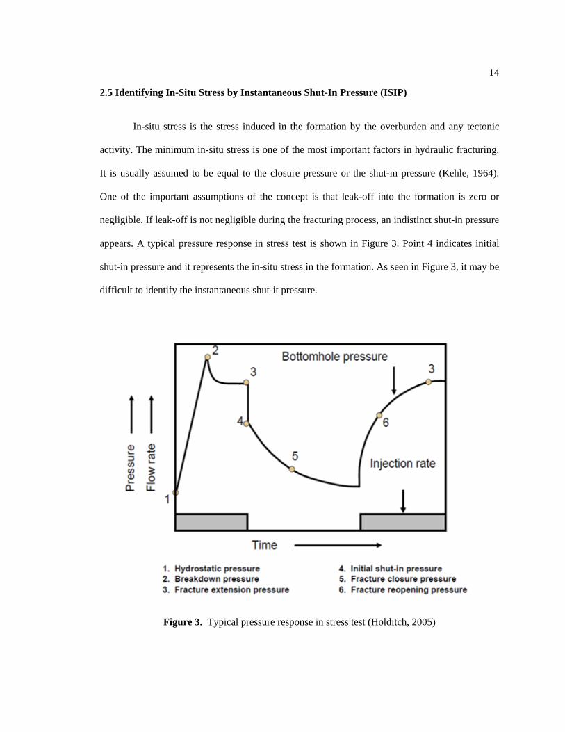
appears. A typical pressure response in stress test is shown in Figure 3. Point 4 indicates initial
shut-in pressure and it represents the in-situ stress in the formation. As seen in Figure 3, it may be
difficult to identify the instantaneous shut-it pressure.
Figure 3. Typical pressure response in stress test (Holditch, 2005)
15
For that reason, numerous methods have been proposed to deal with the indistinct
problem, but the minimum in-situ stress was not measured directly in those tests so it was
difficult to obtain a persuasive conclusion. In 1993, shut-in pressure responses were measured in
a laboratory single-well hydraulic fracturing program by Guo, Morgenstern, and Scott. They
introduced eight methods and validated with the laboratory data, which will be described in the
following paragraphs and used in my model.
Inflection Point Method
This method is a simple graphical technique. The construction is composed of drawing a
tangent line to the pressure-time record right after shut-in (Gronseth and Kry, 1981). The point
where the pressure-time record departs from the straight line is regarded as the shut-in pressure.
p vs. log (t+△t)/△t Method
This method shows that the inflection point of p vs. log (t+△t)/△t plot represents the
shut-in pressure, where p is the bottomhole pressure, t is the injection time, and △t is the time
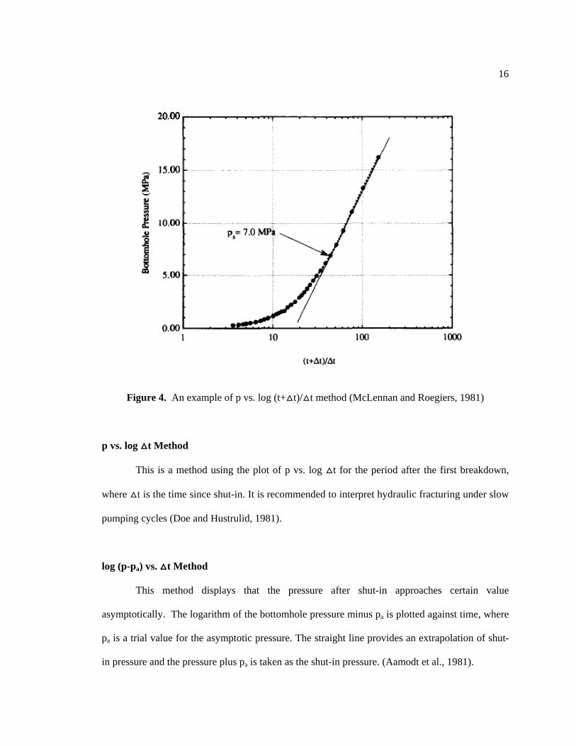
since shut-in (McLennan and Roegiers, 1981). Figure 4 illustrates an example of this method
from hydraulic fracture tests.
16
Figure 4. An example of p vs. log (t+△t)/△t method (McLennan and Roegiers, 1981)
p vs. log △t Method
This is a method using the plot of p vs. log △t for the period after the first breakdown,
where △t is the time since shut-in. It is recommended to interpret hydraulic fracturing under slow
pumping cycles (Doe and Hustrulid, 1981).
log (p-pa) vs. △t Method
This method displays that the pressure after shut-in approaches certain value
asymptotically. The logarithm of the bottomhole pressure minus pa is plotted against time, where
pa is a trial value for the asymptotic pressure. The straight line provides an extrapolation of shut-
in pressure and the pressure plus pa is taken as the shut-in pressure. (Aamodt et al., 1981).
17
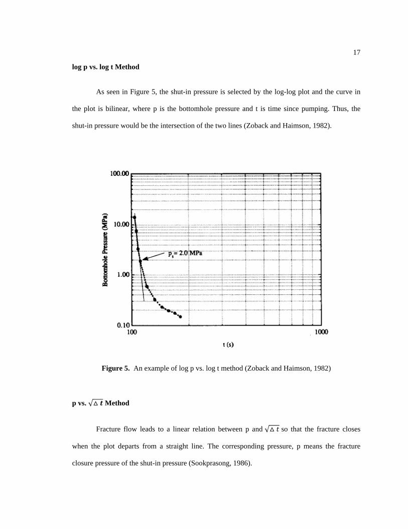
log p vs. log t Method
As seen in Figure 5, the shut-in pressure is selected by the log-log plot and the curve in
the plot is bilinear, where p is the bottomhole pressure and t is time since pumping. Thus, the
shut-in pressure would be the intersection of the two lines (Zoback and Haimson, 1982).
Figure 5. An example of log p vs. log t method (Zoback and Haimson, 1982)
p vs. √△ 𝒕𝒕 Method
Fracture flow leads to a linear relation between p and √△ 𝑛𝑛 so that the fracture closes
when the plot departs from a straight line. The corresponding pressure, p means the fracture
closure pressure of the shut-in pressure (Sookprasong, 1986).

18
dp/dt vs. p Method
It is also assumed that the shut-in curve is bilinear in the plot of dp/dt vs. p, where p is the
bottomhole pressure. This method is illustrated in Figure 6. In this plot, the intersection of the
bilinear lines corresponds to the shut-in pressure (Tunbridge, 1989).
Figure 6. An example of dp/dt vs. p method (Tunbridge, 1989)
Maximum Curvature Method
At the point of maximum curvature in the shut-in curve, the bottomhole pressure is also
recommended as the shut-in pressure. The curvature would depend on the second derivative of
pressure vs. time (Hayashi and Sakurai, 1989).
19
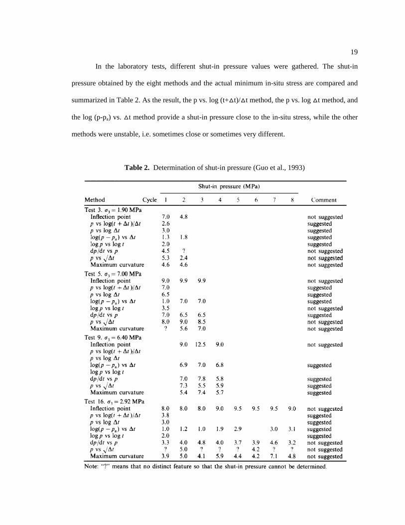
In the laboratory tests, different shut-in pressure values were gathered. The shut-in
pressure obtained by the eight methods and the actual minimum in-situ stress are compared and
summarized in Table 2. As the result, the p vs. log (t+△t)/△t method, the p vs. log △t method, and
the log (p-pa) vs. △t method provide a shut-in pressure close to the in-situ stress, while the other
methods were unstable, i.e. sometimes close or sometimes very different.
Table 2. Determination of shut-in pressure (Guo et al., 1993)

20
Chapter 3
STATEMENT OF THE PROBLEM
Real-time field data generated during the fracture treatment include surface treating
pressure, flow rate, and fluid density, so it is very difficult to interpret hydraulic fracturing
pressure without accurate calculation of bottomhole treating pressure. The objectives of my study
are to calculate bottomhole treating pressure and net pressure accurately and to develop new
methods to interpret fracture geometry and formation properties.
New models for the accurate calculation of bottomhole treating pressure and net pressure
will be developed in Chapter 4. This calculation is determined by considering pertinent factors
such as fracture fluid property changes along the wellbore, effect of near wellbore pressures,
proppant effect, casing toughness, rock toughness, thermal effect, and pore pressure effect. New
methods will be introduced for more accurate interpretation of the bottomhole treating pressure
and net pressure. The new models and methods will be validated with field data.
The procedure of my research is outlined below:
1. Complete a literature review of all mathematical models, laboratory experiments,
and field data related to the interpretation of hydraulic fracturing pressure.
2. Develop mathematical models to characterize how the fracture fluids flow down
the wellbore/tubing, flow through perforations, leak off into reservoir, and prop
open formation rock.
3. Develop a fit-for-purpose model for accurate estimation of bottomhole treating
pressure, in-situ stress, and net pressure.

21
4. Develop new methods for interpretation of fracture geometry and formation
properties in low-permeability gas formation.
5. Document new findings into a thesis and papers.
22
Chapter 4
MODEL DEVELOPMENT AND VALIDATIONS
4.1 Fracture Fluid Density Change along the Wellbore
The density data used for the calculation of bottomhole treating pressure came from
density data at the surface. For a fracturing fluid injected into the wellbore, however, density of
the fluid increases with depth as pressure increased.
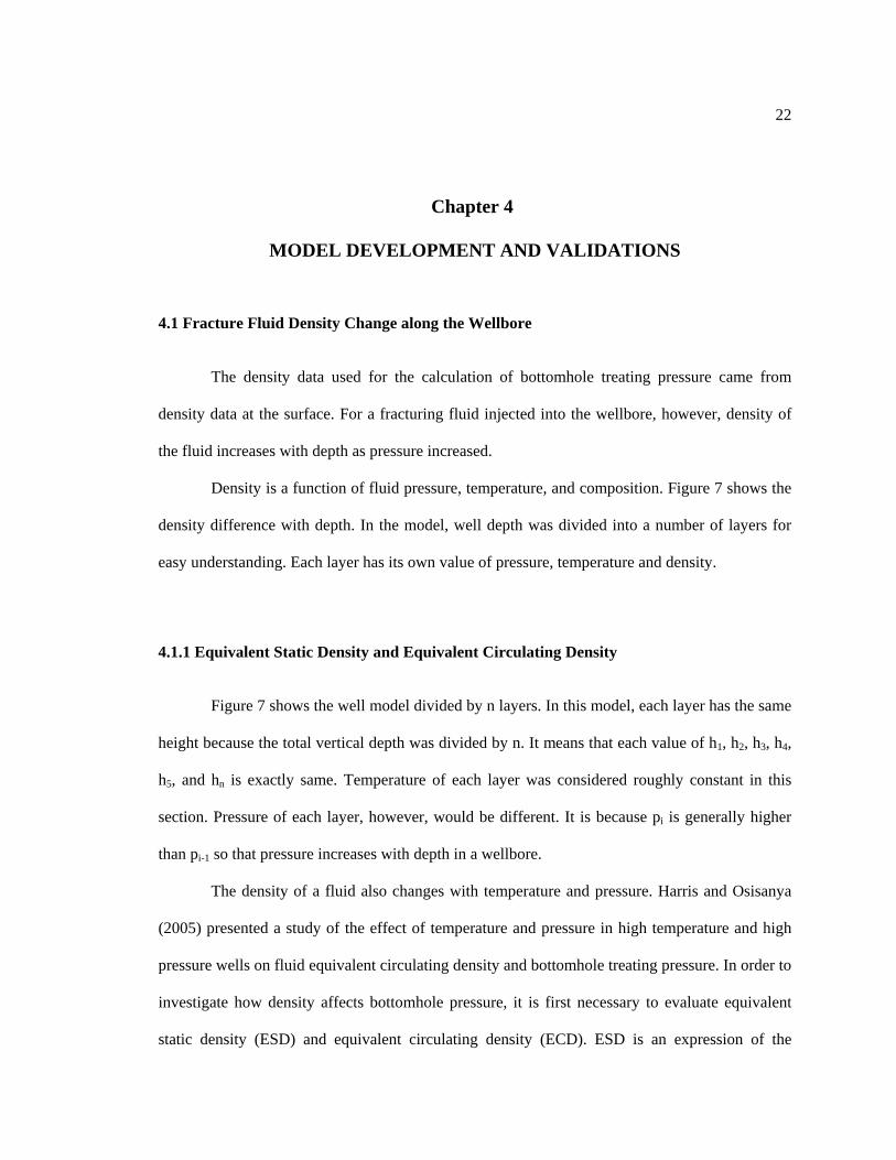
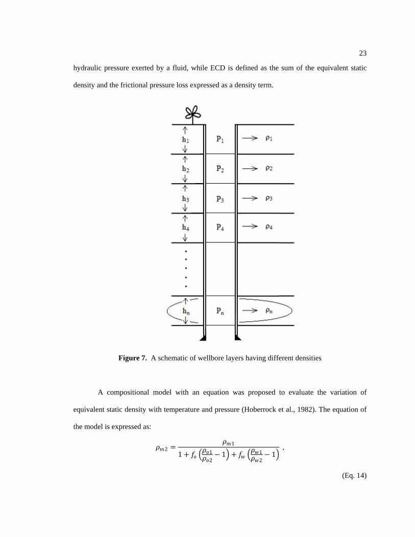
Density is a function of fluid pressure, temperature, and composition. Figure 7 shows the
density difference with depth. In the model, well depth was divided into a number of layers for
easy understanding. Each layer has its own value of pressure, temperature and density.
4.1.1 Equivalent Static Density and Equivalent Circulating Density
Figure 7 shows the well model divided by n layers. In this model, each layer has the same
height because the total vertical depth was divided by n. It means that each value of h1, h2, h3, h4,
h5, and hn is exactly same. Temperature of each layer was considered roughly constant in this
section. Pressure of each layer, however, would be different. It is because pi is generally higher
than pi-1 so that pressure increases with depth in a wellbore.
The density of a fluid also changes with temperature and pressure. Harris and Osisanya
(2005) presented a study of the effect of temperature and pressure in high temperature and high
pressure wells on fluid equivalent circulating density and bottomhole treating pressure. In order to
investigate how density affects bottomhole pressure, it is first necessary to evaluate equivalent
static density (ESD) and equivalent circulating density (ECD). ESD is an expression of the
23
hydraulic pressure exerted by a fluid, while ECD is defined as the sum of the equivalent static
density and the frictional pressure loss expressed as a density term.
Figure 7. A schematic of wellbore layers having different densities
A compositional model with an equation was proposed to evaluate the variation of
equivalent static density with temperature and pressure (Hoberrock et al., 1982). The equation of
the model is expressed as:
𝜌𝜌𝑚𝑚2 =𝜌𝜌𝑚𝑚1
1 + 𝑠𝑠𝑐𝑐 �𝜌𝜌𝑐𝑐1𝜌𝜌𝑐𝑐2
− 1� + 𝑠𝑠𝑤𝑤 �𝜌𝜌𝑤𝑤1𝜌𝜌𝑤𝑤2
− 1� ,
(Eq. 14)
24
where
ρm1 = mud density at reference conditions, lb/gal,
ρm2 = mud density at elevated temperature and pressure, lb/gal,
ρo1, ρw1 = oil and water density at reference conditions, lb/gal,
ρo2, ρw2 = oil and water density at elevated temperature and pressure, lb/gal, and
fo, fw = volume fractions of oil and water.
The model proposed above assumes that any density change of a fluid as a result of
temperature and pressure change comes from the volumetric behavior of its liquid components
that will be constituents of water and oil. To find densities at elevated pressure and temperature
(ρo2, ρw2) the model requires volumetric behavior of the liquid constituents.
Politte (1985) expressed the volumetric behavior of oil and developed the following
empirical equation from analysis of diesel oil No. 2.
𝜌𝜌𝑐𝑐(𝑝𝑝𝑓𝑓 ,𝑇𝑇𝑓𝑓) = 𝐶𝐶0 + 𝐶𝐶1 ∗ 𝑝𝑝𝑓𝑓𝑇𝑇𝑓𝑓 + 𝐶𝐶2 ∗ 𝑝𝑝𝑓𝑓 + 𝐶𝐶3 ∗ 𝑝𝑝𝑓𝑓2 + 𝐶𝐶4 ∗ 𝑇𝑇𝑓𝑓 + 𝐶𝐶5 ∗ 𝑇𝑇𝑓𝑓2 ,
(Eq. 15)
where C0 = 0.8807 C1 = 1.5235*10-9
C2 = 1.2806*10-6 C3 = 1.0719*10-10
C4 = -0.00036 C5 = -5.1670*10-8.
pi is the pressure at i-th layer in psi, Ti is the temperature at i-th layer in °F, and C0, C1,
C2, C3, C4, and C5 are empirical constants. An equation for the volumetric behavior of water was
also developed by Sorelle et al. (1982). It was obtained by curve fitting data from tables of
physical properties of water. The density of water can be expressed as:
25
𝜌𝜌𝑤𝑤(𝑝𝑝𝑓𝑓 ,𝑇𝑇𝑓𝑓) = 𝐷𝐷0 + 𝐷𝐷1 ∗ 𝑇𝑇𝑓𝑓 + 𝐷𝐷2 ∗ 𝑝𝑝𝑓𝑓 ,
(Eq. 16)
where D0 = 8.63186 D1 = -3.31877*10-3
D2 = 2.3717*10-5.
D0, D1, and D2 are empirical constants. Fluid densities for each layer, from ρ1 to ρn, can be
obtained by using those density equations.
4.1.2 Applications to Field Data
This model was applied to two sets of field data, which were donated by Sklar
Exploration Company (2008). In order to display each plot clearer, time during the test period
was not shown. Therefore, elapsed time will start right after the main treatment for each case
study.
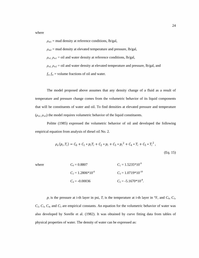
For the improved density calculation, the depth was divided into 10 layers (n=10). In
addition, each layer had the same height and constant temperature. However, hydrostatic pressure
will be different for each layer due to density changes. The new density equation mentioned
above was used for the hydrostatic pressure calculation. The results would be presented as plots
of hydrostatic pressure vs. elapsed time in Figures 8 and 9.
4.1.3 Results and Validations
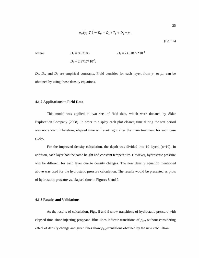
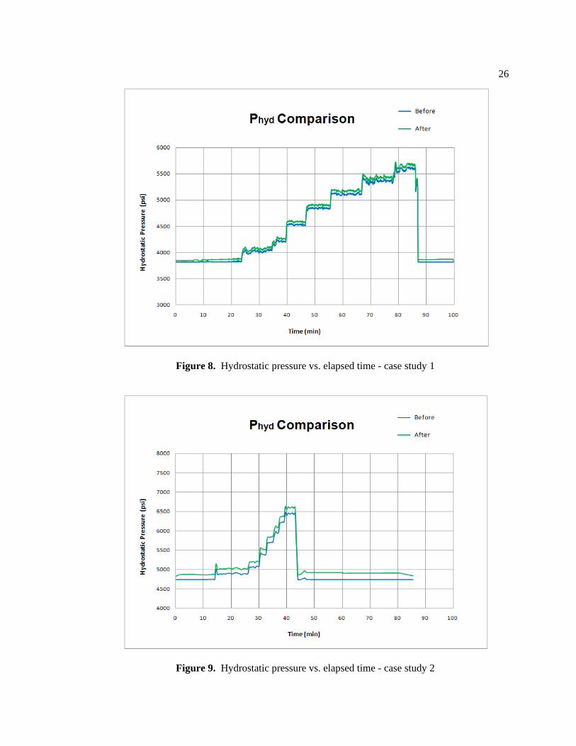
As the results of calculation, Figs. 8 and 9 show transitions of hydrostatic pressure with
elapsed time since injecting proppant. Blue lines indicate transitions of phyd without considering
effect of density change and green lines show phyd transitions obtained by the new calculation.
26
Figure 8. Hydrostatic pressure vs. elapsed time - case study 1
Figure 9. Hydrostatic pressure vs. elapsed time - case study 2

27
From the plots, we are able to find distinct changes. The hydrostatic pressure in the new
model is obviously higher than that of the old. Two case studies present the same result. This is
because the density of each layer increases as it goes deeper. The average increment of phyd for
case study 1 was 54.3 psi and the average pressure increment for case study 2 was 131.7psi. Such
a difference between two cases is due to depth difference (i.e. well depth of case 2 is deeper than
that of case 1). The increased density makes hydrostatic pressure higher and the increased
hydrostatic pressure will make BHTP increase, too. With this result, it shows that density change
of a fluid affects the bottomhole pressure calculation and needs to be considered.
28
4.2 Effect of Casing Roughness
Roughness of casing can be defined as a measure of the texture of the surface inside a
pipe. Casing roughness plays an important role in determining how the pipe will interact with
fluid flow. In general, rough surfaces have higher friction coefficients than smooth surfaces.
Therefore, it should be considered how roughness of the pipe affects frictional pressure loss for
this section.
4.2.1 Fanning Friction Factor
Fanning friction factor is one-fourth of the Darcy friction factor, so attention must be paid
to check which is being used in the friction factor equation. Of the two, the Fanning friction
factor is the more commonly used in the petroleum engineering field because in the case of the
Darcy equation, no electronic calculators are available and many calculations have to be carried
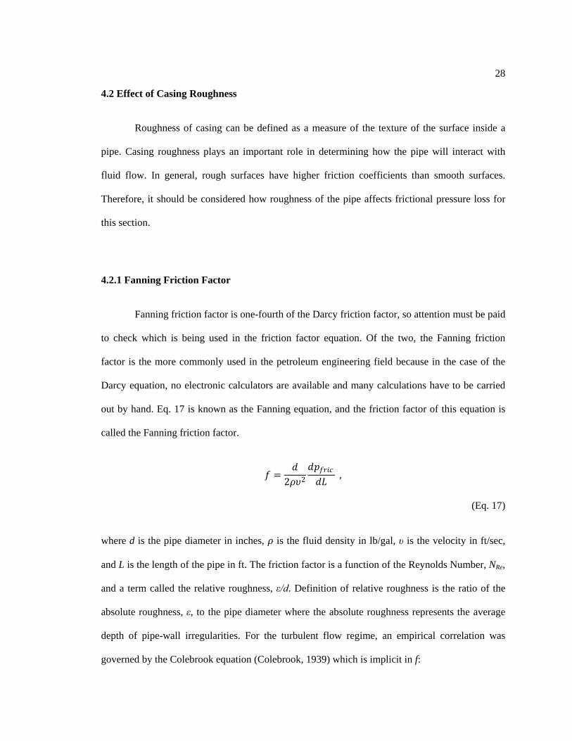
out by hand. Eq. 17 is known as the Fanning equation, and the friction factor of this equation is
called the Fanning friction factor.
𝑠𝑠 =𝑦𝑦
2𝜌𝜌𝜌𝜌2𝑦𝑦𝑝𝑝𝑠𝑠𝑠𝑠𝑓𝑓𝑐𝑐𝑦𝑦𝐿𝐿
,
(Eq. 17)
where d is the pipe diameter in inches, 𝜌𝜌 is the fluid density in lb/gal, υ is the velocity in ft/sec,
and L is the length of the pipe in ft. The friction factor is a function of the Reynolds Number, NRe,
and a term called the relative roughness, ε/d. Definition of relative roughness is the ratio of the
absolute roughness, ε, to the pipe diameter where the absolute roughness represents the average
depth of pipe-wall irregularities. For the turbulent flow regime, an empirical correlation was
governed by the Colebrook equation (Colebrook, 1939) which is implicit in f:
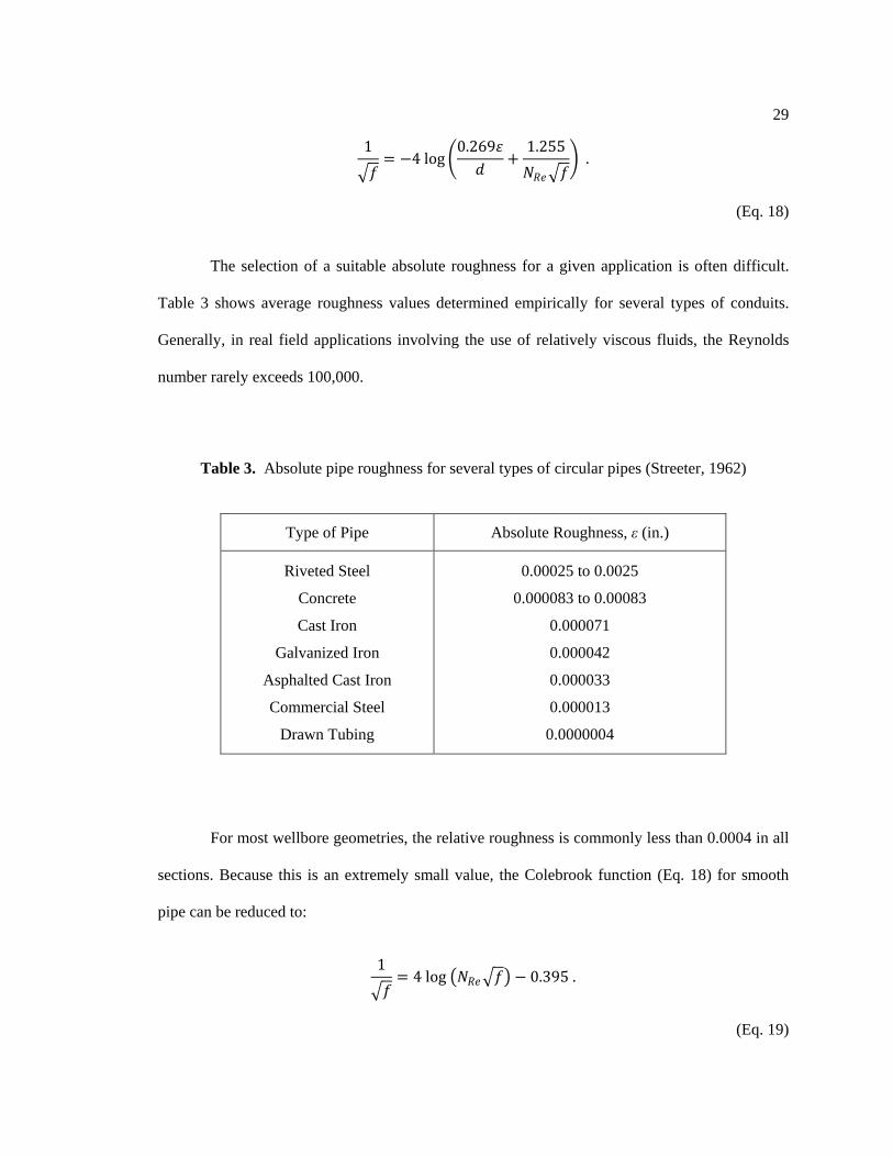
29
1�𝑠𝑠
= −4 log �0.269𝜀𝜀𝑦𝑦
+1.255𝑁𝑁𝑅𝑅𝑛𝑛�𝑠𝑠
� .
(Eq. 18)
The selection of a suitable absolute roughness for a given application is often difficult.
Table 3 shows average roughness values determined empirically for several types of conduits.
Generally, in real field applications involving the use of relatively viscous fluids, the Reynolds
number rarely exceeds 100,000.
Table 3. Absolute pipe roughness for several types of circular pipes (Streeter, 1962)
Type of Pipe Absolute Roughness, ε (in.)
Riveted Steel
Concrete
Cast Iron
Galvanized Iron
Asphalted Cast Iron
Commercial Steel
Drawn Tubing
0.00025 to 0.0025
0.000083 to 0.00083
0.000071
0.000042
0.000033
0.000013
0.0000004
For most wellbore geometries, the relative roughness is commonly less than 0.0004 in all
sections. Because this is an extremely small value, the Colebrook function (Eq. 18) for smooth
pipe can be reduced to:
1�𝑠𝑠
= 4 log �𝑁𝑁𝑅𝑅𝑛𝑛�𝑠𝑠� − 0.395 .
(Eq. 19)
30
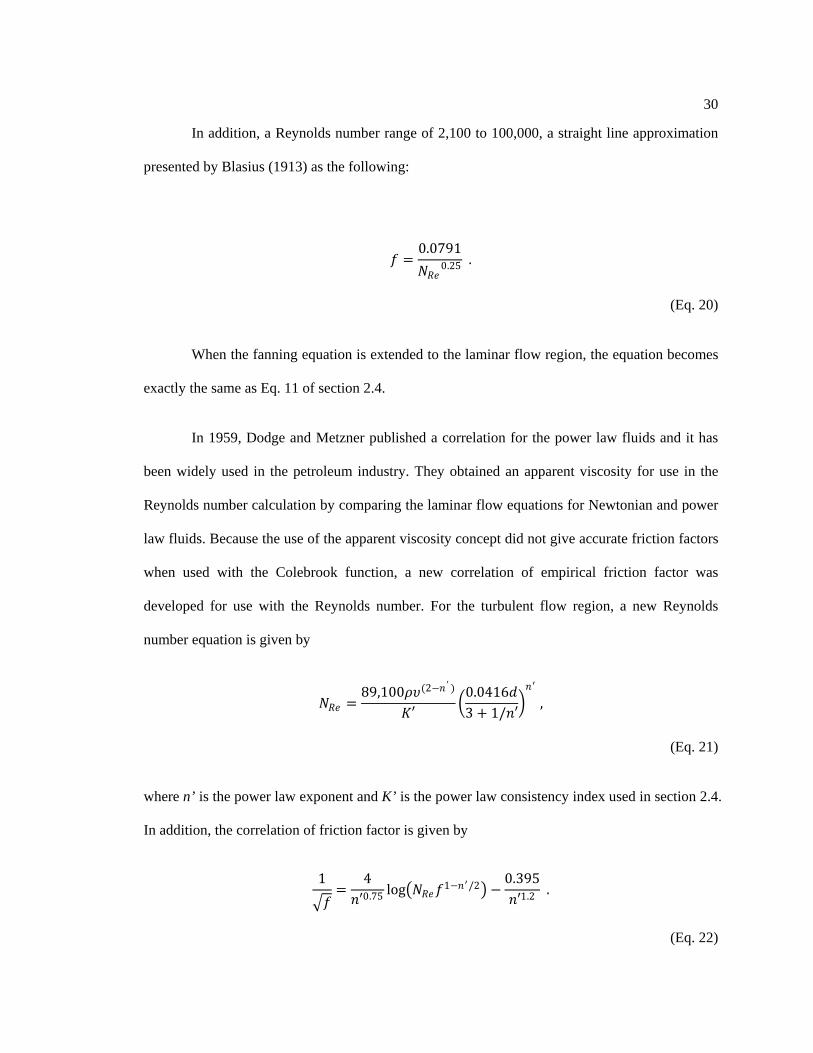
In addition, a Reynolds number range of 2,100 to 100,000, a straight line approximation
presented by Blasius (1913) as the following:
𝑠𝑠 =0.0791𝑁𝑁𝑅𝑅𝑛𝑛0.25 .
(Eq. 20)
When the fanning equation is extended to the laminar flow region, the equation becomes
exactly the same as Eq. 11 of section 2.4.
In 1959, Dodge and Metzner published a correlation for the power law fluids and it has
been widely used in the petroleum industry. They obtained an apparent viscosity for use in the
Reynolds number calculation by comparing the laminar flow equations for Newtonian and power
law fluids. Because the use of the apparent viscosity concept did not give accurate friction factors
when used with the Colebrook function, a new correlation of empirical friction factor was
developed for use with the Reynolds number. For the turbulent flow region, a new Reynolds
number equation is given by
𝑁𝑁𝑅𝑅𝑛𝑛 =89,100𝜌𝜌𝜌𝜌(2−𝑛𝑛′ )
𝐾𝐾′�
0.0416𝑦𝑦3 + 1/𝑛𝑛′
�𝑛𝑛′
,
(Eq. 21)
where n’ is the power law exponent and K’ is the power law consistency index used in section 2.4.
In addition, the correlation of friction factor is given by
1�𝑠𝑠
=4
𝑛𝑛′0.75 log�𝑁𝑁𝑅𝑅𝑛𝑛𝑠𝑠1−𝑛𝑛′/2� −0.395𝑛𝑛′1.2 .
(Eq. 22)
31
The correlation was developed only for smooth pipe. However, there is no strict
limitation for most fracture fluid applications. A graphical representation of Eq. 22 is shown in
Appendix B. As seen in Figure B.2, the upper line is for n’=1 and is identical to the smooth
pipeline on Figure B.1.
4.2.2 Applications to Field Data
This model is applied to the same case studies in the previous section. For the case where
the Reynolds number is greater than 2,100, the flow pattern would be turbulent. The absolute
roughness is given in Table 3. For our model, commercial steel is applied because it is the most
used in the field (Bourgoyne et al., 1986), so the relative roughness can easily be calculated.
Thus, solving Eq. 22 by trial and error, the Fanning friction factor can be obtained.
4.2.3 Results and Validations
Fortunately, for most wellbore geometries, the Fanning friction factors for smooth pipe
are assumed to have zero roughness and can be applied for most engineering calculations. That is
because the relative roughness is usually less than 0.0004 (Bourgoyne et al., 1986). Therefore, the
relative roughness can be ignored when we calculate the Fanning friction factor. After using new
equations, the result did not give salient change of frictional pressure drop. This means that the
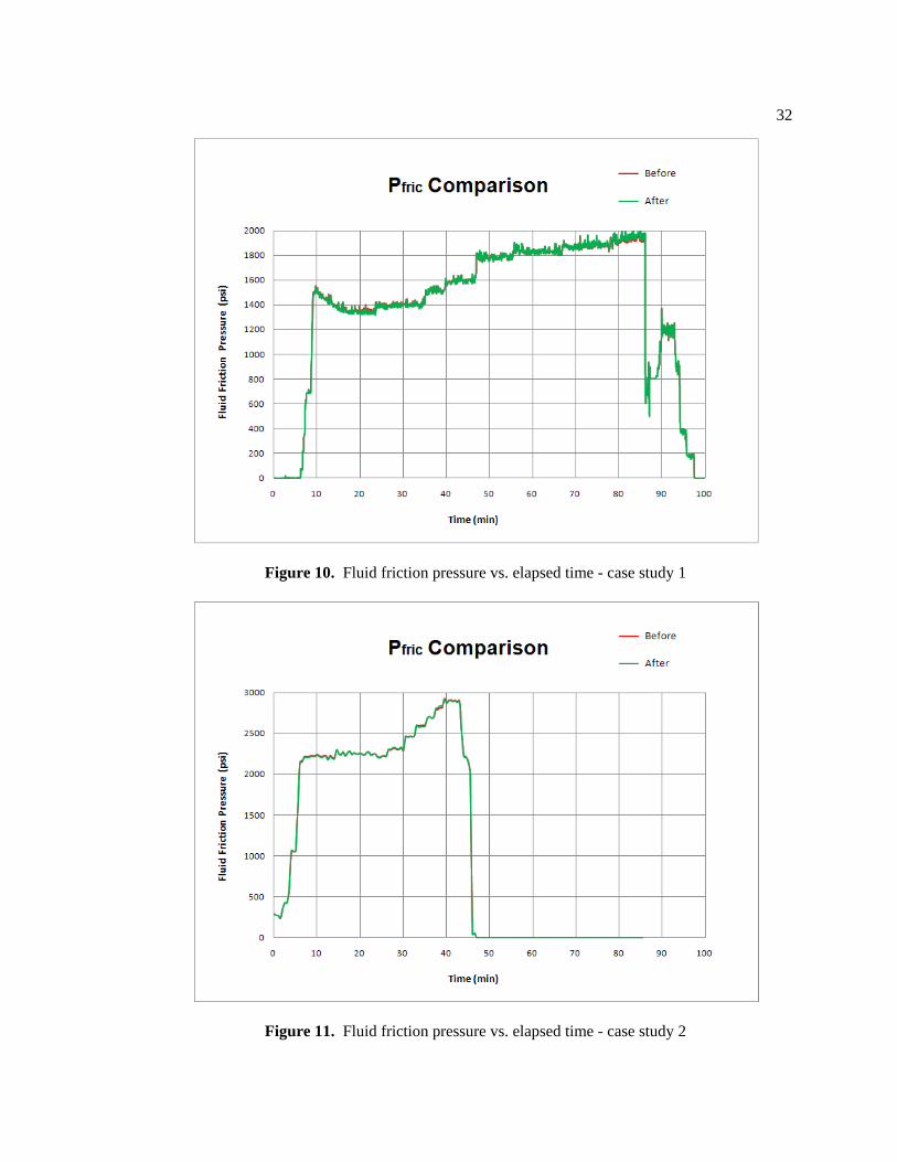
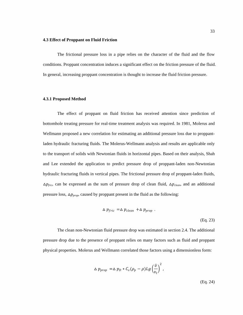
effect of casing roughness can be negligible for the fluid friction pressure calculation. Figures 10
and 11 show the result.
32
Figure 10. Fluid friction pressure vs. elapsed time - case study 1
Figure 11. Fluid friction pressure vs. elapsed time - case study 2
33
4.3 Effect of Proppant on Fluid Friction
The frictional pressure loss in a pipe relies on the character of the fluid and the flow
conditions. Proppant concentration induces a significant effect on the friction pressure of the fluid.
In general, increasing proppant concentration is thought to increase the fluid friction pressure.
4.3.1 Proposed Method
The effect of proppant on fluid friction has received attention since prediction of
bottomhole treating pressure for real-time treatment analysis was required. In 1981, Molerus and
Wellmann proposed a new correlation for estimating an additional pressure loss due to proppant-
laden hydraulic fracturing fluids. The Molerus-Wellmann analysis and results are applicable only
to the transport of solids with Newtonian fluids in horizontal pipes. Based on their analysis, Shah
and Lee extended the application to predict pressure drop of proppant-laden non-Newtonian
hydraulic fracturing fluids in vertical pipes. The frictional pressure drop of proppant-laden fluids,
△pfric, can be expressed as the sum of pressure drop of clean fluid, △pclean, and an additional
pressure loss, △pprop, caused by proppant present in the fluid as the following:
△ 𝑝𝑝𝑠𝑠𝑠𝑠𝑓𝑓𝑐𝑐 =△ 𝑝𝑝𝑐𝑐𝑐𝑐𝑛𝑛𝑐𝑐𝑛𝑛 +△ 𝑝𝑝𝑝𝑝𝑠𝑠𝑐𝑐𝑝𝑝 .
(Eq. 23)
The clean non-Newtonian fluid pressure drop was estimated in section 2.4. The additional
pressure drop due to the presence of proppant relies on many factors such as fluid and proppant
physical properties. Molerus and Wellmann correlated those factors using a dimensionless form:
△ 𝑝𝑝𝑝𝑝𝑠𝑠𝑐𝑐𝑝𝑝 =△ 𝑝𝑝𝐷𝐷 ∗ 𝐶𝐶𝜌𝜌(𝜌𝜌𝑝𝑝 − 𝜌𝜌)𝐿𝐿𝐿𝐿 ��̅�𝜌𝜌𝜌𝑛𝑛�
2 ,
(Eq. 24)
34
where
△pprop = additional pressure drop caused by proppant in fluid, psi,
△pD = dimensionless pressure drop parameter, psi,
Cυ = frictional volumetric concentration of proppants,
𝜌𝜌 = fluid density
𝜌𝜌p = particle density, lb/gal,
L = length of pipe, ft,
g = gravitational acceleration, ft/sec2.
�̅�𝜌 = mean suspension velocity, ft/sec, and
𝜌𝜌t = single particle-settling velocity, ft/sec.
In addition, △pD and Cυ can be expressed as:
△ 𝑝𝑝𝐷𝐷 =(�̅�𝜌𝑐𝑐/�̅�𝜌)2
1 − (�̅�𝜌𝑐𝑐/�̅�𝜌)
(Eq. 25)
and
𝐶𝐶𝜌𝜌 = (𝜌𝜌𝑐𝑐 − 𝜌𝜌)/�𝜌𝜌𝑝𝑝 − 𝜌𝜌� ,
(Eq. 26)
where 𝜌𝜌s is the slurry density in lb/gal and �̅�𝜌𝑐𝑐 is the mean slip velocity of the particles relative to
the mean suspension velocity, �̅�𝜌. In addition, (�̅�𝜌𝑐𝑐/�̅�𝜌) of the △pD calculation can be obtained by
specified empirical data (Shah and Lee, 1986). This correlation was developed with various
concentrations of HPG solutions; its generality to other types of solutions has not been
demonstrated yet.
35
4.3.2 Applications to Field Data
We already dealt with an equation of fluid friction pressure in section 2.4, but it is
actually the friction pressure equation only for the clean fluid. Therefore, the additional pressure
loss due to proppant effect has to be added by using Eq. 24. The result will present frictional
pressure differences between the old model and the new model.
4.3.3 Results and Validations
As seen in Figures 12 and 13, fluid friction pressure increased slightly for both case
studies after applying the new model with proppant effect. This implies that the additional friction
loss due to the proppant effect increases the total fluid frictional loss. For case study 1, the
average friction pressure loss due to proppant effect was 24.9 psi and the average pressure loss
for case study 2 was 19.5 psi.
36
Figure 12. Effect of proppant on friction pressure vs. elapsed time - case study 1
Figure 13. Effect of proppant on friction pressure vs. elapsed time - case study 2
37
4.4 Effect of Near-Wellbore Friction
Near-wellbore friction is a general term designed to include a number of effects that
restrict the flow between the wellbore and the main body of the fracture. Near-wellbore friction
pressure definitely affects calculation of bottomhole treating pressure and net pressure. It is very
important to identify near-wellbore friction since its region is usually composed of complex
pathways connecting the wellbore with the main body of the fracture so that it becomes an
indicator of fracture pressure analysis.
Near-wellbore friction pressure is the total pressure lost by near-wellbore effects and it
can be quantified as the sum of the pressure drop caused by perforation friction and tortuosity. In
this section, we will go through the perforation friction pressure and the tortuosity pressure
separately.
4.4.1 Perforation Pressure Loss
It is essential to estimate the perforation friction drop in order to identify the near-
wellbore friction pressure. In the BHTP calculation, this frictional loss is sometimes assumed to
be zero or negligible since the calculation is complicated and depends upon empirical sources like
laboratory data. The friction pressure drop across the perforations is generally expressed by the
following equation.
∆𝑝𝑝𝑝𝑝𝑛𝑛𝑠𝑠𝑠𝑠 =0.2369𝑞𝑞2𝜌𝜌𝑁𝑁𝑝𝑝2𝑦𝑦𝑝𝑝
4𝐶𝐶𝑦𝑦2 ,
(Eq. 27)
where
∆𝑝𝑝𝑝𝑝𝑛𝑛𝑠𝑠𝑠𝑠 = perforations friction pressure loss, psi,
𝑞𝑞 = total flow rate, bbl/min,
38
𝜌𝜌 = fluid density, lb/gal,
𝑁𝑁𝑝𝑝 = number of perforations,
𝑦𝑦𝑝𝑝 = initial perforation diameter, in., and
𝐶𝐶𝑦𝑦 = coefficient of discharge.
In this equation, there is a kinetic energy correction factor, which is known as the
‘coefficient of discharge (𝐶𝐶𝑦𝑦 ).’ Coefficient of discharge is the ratio of the diameter of the fluid
stream at the vena contracta (point of lowest pressure drop) to the diameter of the perforation as
shown in Figure 14. It is difficult to estimate perforation friction pressure since the coefficient
discharge changes due to perforation erosion and it cannot be determined unless the exact cross-
sectional area is known, while the other parameters are easily obtained by real-time field data
such as the fluid flow rate and the fluid density.
Figure 14. A schematic of orifice-square edge (Willingham et al., 1993)

39
Recent studies have proved that the discharge coefficient can significantly change with
perforation size and viscosity of fluids. New reliable correlations of perforation pressure loss for
fracturing treatment were developed to estimate the coefficient of discharge used in the orifice
equation that governs the perforation pressure loss (El-Rabba and Shah, 1999). The correlations
were used to accurately predict the discharge coefficient for linear polymer solutions and
titanium-crosslinked gels. In addition, a correlation was also presented to determine the
unpredictable change in the discharge coefficient for fracturing slurries due to erosion.
For clean fluids
A new coefficient of discharge based on the statistical analysis was developed for both
HPG and titanium-crosslinked HPG as follows:
For linear HPG,
𝐶𝐶𝑦𝑦 = �1 − 𝑛𝑛−2.2𝑦𝑦𝑠𝑠𝑑𝑑𝑐𝑐 0.1 �
0.4
, 𝑠𝑠2 = 0.886 .
(Eq. 28)
For Titanium-crosslinked HPG,
𝐶𝐶𝑦𝑦 = �1 − 𝑛𝑛−1.76
(𝑑𝑑𝑐𝑐𝑦𝑦𝑝𝑝 )0.25�0.6
, 𝑠𝑠2 = 0.962 ,
(Eq. 29)
where
𝐶𝐶𝑦𝑦= coefficient of discharge,
𝑦𝑦𝑝𝑝 = initial perforation diameter, in.,
𝑑𝑑𝑐𝑐 = apparent viscosity of linear polymer solution, cp, and
𝑠𝑠2 = correlation coefficient.
40
For sand slurries
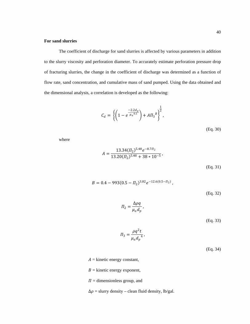
The coefficient of discharge for sand slurries is affected by various parameters in addition
to the slurry viscosity and perforation diameter. To accurately estimate perforation pressure drop
of fracturing slurries, the change in the coefficient of discharge was determined as a function of
flow rate, sand concentration, and cumulative mass of sand pumped. Using the data obtained and
the dimensional analysis, a correlation is developed as the following:
𝐶𝐶𝑦𝑦 = ��1 − 𝑛𝑛−2.2𝑦𝑦𝑝𝑝𝑑𝑑𝑐𝑐 0.1 � + 𝐴𝐴𝛱𝛱3
𝐵𝐵�
12
,
(Eq. 30)
where
𝐴𝐴 =13.34(𝛱𝛱2)5.48𝑛𝑛−8.7𝛱𝛱2
13.20(𝛱𝛱2)5.48 + 38 ∗ 10−5 ,
(Eq. 31)
𝐵𝐵 = 0.4 − 993(0.5 − 𝛱𝛱2)3.82𝑛𝑛−12.6(0.5−𝛱𝛱2) ,
(Eq. 32)
𝛱𝛱2 =∆𝜌𝜌𝑞𝑞𝑑𝑑𝑐𝑐𝑦𝑦𝑝𝑝
,
(Eq. 33)
𝛱𝛱3 =𝜌𝜌𝑞𝑞2𝑛𝑛𝑑𝑑𝑐𝑐𝑦𝑦𝑝𝑝
4 ,
(Eq. 34)
𝐴𝐴 = kinetic energy constant,
𝐵𝐵 = kinetic energy exponent,
𝛱𝛱 = dimensionless group, and
∆𝜌𝜌 = slurry density – clean fluid density, lb/gal.
41
It is important to note that the discharge coefficient will be designated by the linear
polymer solution correlation as sand concentration goes near zero. With any empirical
correlations, the correlations shown above are valid for the range of variables considered.
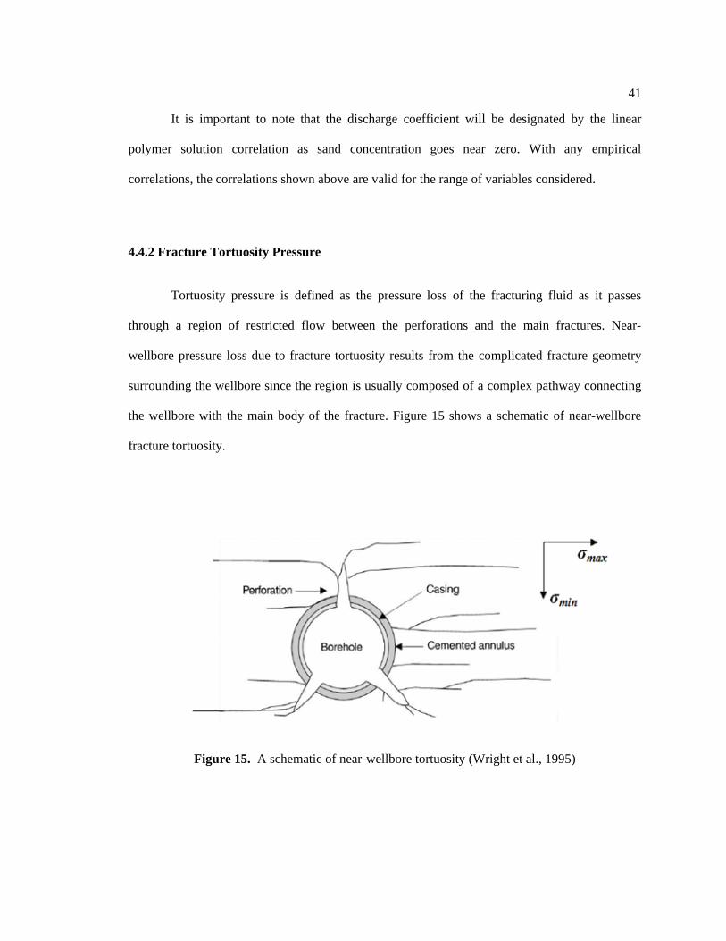
4.4.2 Fracture Tortuosity Pressure
Tortuosity pressure is defined as the pressure loss of the fracturing fluid as it passes
through a region of restricted flow between the perforations and the main fractures. Near-
wellbore pressure loss due to fracture tortuosity results from the complicated fracture geometry
surrounding the wellbore since the region is usually composed of a complex pathway connecting
the wellbore with the main body of the fracture. Figure 15 shows a schematic of near-wellbore
fracture tortuosity.
Figure 15. A schematic of near-wellbore tortuosity (Wright et al., 1995)
42
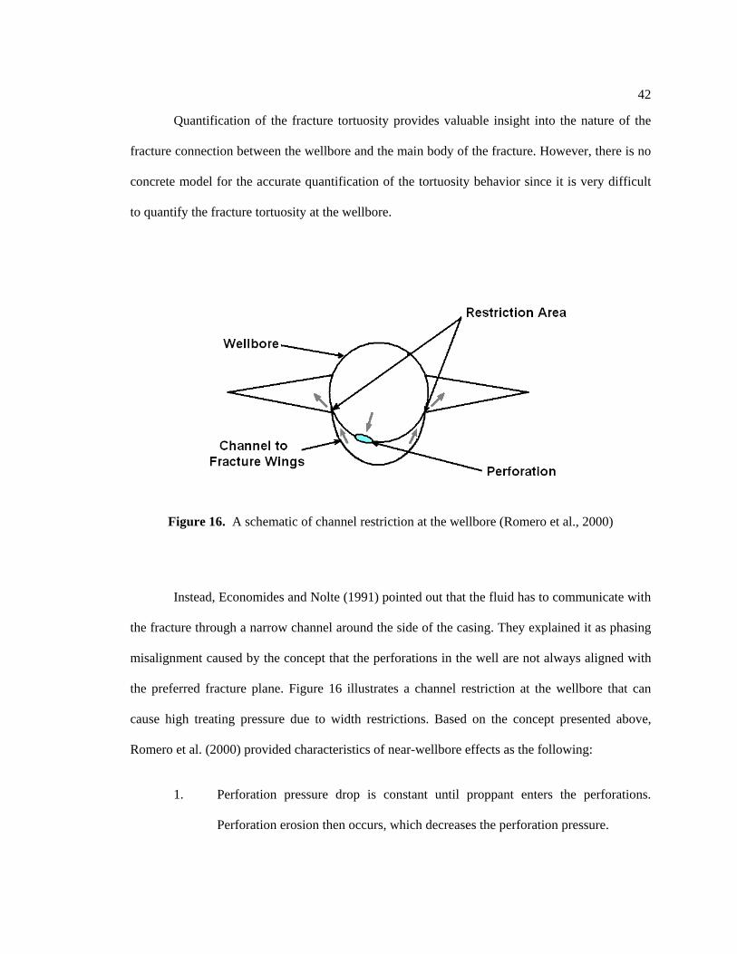
Quantification of the fracture tortuosity provides valuable insight into the nature of the
fracture connection between the wellbore and the main body of the fracture. However, there is no
concrete model for the accurate quantification of the tortuosity behavior since it is very difficult
to quantify the fracture tortuosity at the wellbore.
Figure 16. A schematic of channel restriction at the wellbore (Romero et al., 2000)
Instead, Economides and Nolte (1991) pointed out that the fluid has to communicate with
the fracture through a narrow channel around the side of the casing. They explained it as phasing
misalignment caused by the concept that the perforations in the well are not always aligned with
the preferred fracture plane. Figure 16 illustrates a channel restriction at the wellbore that can
cause high treating pressure due to width restrictions. Based on the concept presented above,
Romero et al. (2000) provided characteristics of near-wellbore effects as the following:
1. Perforation pressure drop is constant until proppant enters the perforations.
Perforation erosion then occurs, which decreases the perforation pressure.
43
2. Tortuosity friction is largest at the beginning of a treatment, and decreases during
the treatment, even without proppant.
3. Perforation misalignment pressure drop can increase as the treatment proceeds if
little or no erosion occurs. The erosion can occur with proppant, and possibly
even with clean fluid.
4.4.3 Applications to Field Data
The model with effect of near-wellbore pressures was applied into two sets of field data
used in previous sections. In this section, the application was only focused on the calculation of
perforation friction pressure since there are no models available to quantify tortuosity pressure.
However, the near-wellbore tortuosity can sometimes cause BHTP to increase significantly when
the fluid flow rate rapidly changes during the fracturing process.
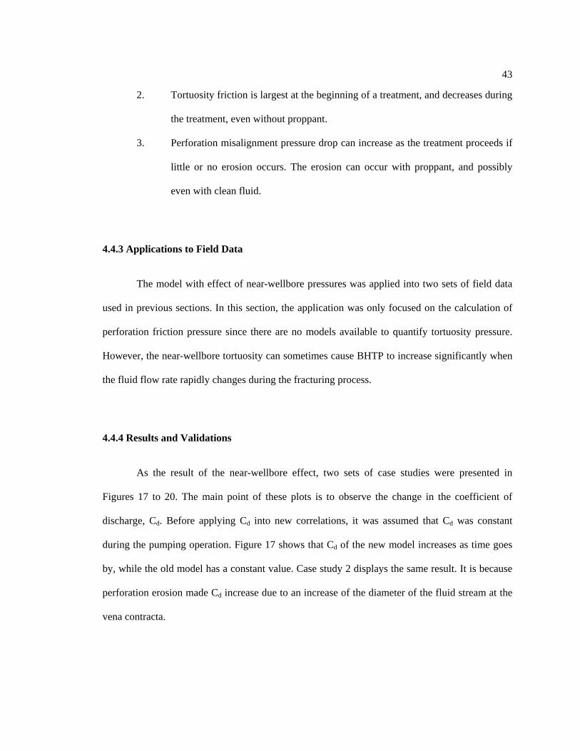
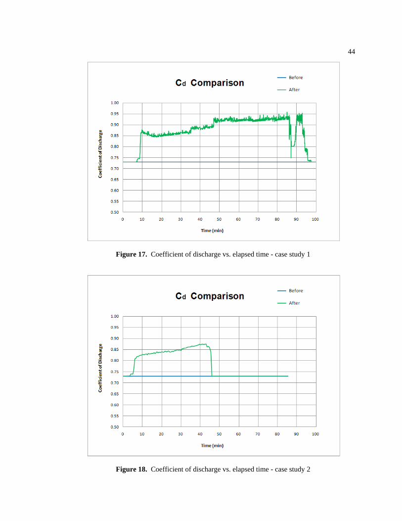
4.4.4 Results and Validations
As the result of the near-wellbore effect, two sets of case studies were presented in
Figures 17 to 20. The main point of these plots is to observe the change in the coefficient of
discharge, Cd. Before applying Cd into new correlations, it was assumed that Cd was constant
during the pumping operation. Figure 17 shows that Cd of the new model increases as time goes
by, while the old model has a constant value. Case study 2 displays the same result. It is because
perforation erosion made Cd increase due to an increase of the diameter of the fluid stream at the
vena contracta.
44
Figure 17. Coefficient of discharge vs. elapsed time - case study 1
Figure 18. Coefficient of discharge vs. elapsed time - case study 2

45
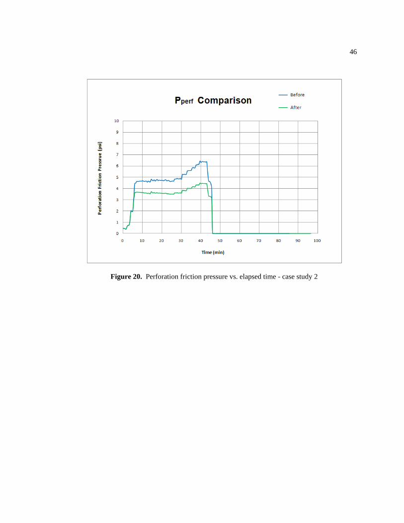
As presented before, the equation of perforation friction pressure shows that coefficient
of discharge is inversely proportional to perforation friction pressure drop. Thus, increase of
discharge coefficient will cause the perforation pressure to decrease. On the other hand, decrease
of the perforation friction loss will make fracture fluid pressure increase. The result of the new
model explains changes of perforation friction pressure in Figures 19 and 20. The figure shows
that perforation friction pressure of the new model is higher than that of the old one. Thus, the
effect of near-wellbore perforation friction can be validated.
Figure 19. Perforation friction pressure vs. elapsed time - case study 1
46
Figure 20. Perforation friction pressure vs. elapsed time - case study 2
47
4.5 Effect of Rock Toughness
In hydraulic fracturing, fracture toughness of rock stands for the amount of energy
required to physically split the rock apart at the fracture tip. It is also known as a critical value of
stress intensity factor, KIc, which presents the resistance of the materials. Since fracture toughness
is a material property, it is generally affected by the temperature of the formation, loading rate,
the composition of the material and its microstructure with geometric effects. It is also influenced
by breakdown pressure using a linear elastic fracture mechanics approach. Increases in rock
toughness usually result in increasing the breakdown pressure (Amadei and Stephansson, 1997).
4.5.1 Stress Intensity Factor
In fracture mechanics, cracks or fractures are usually discovered in various types. From a
mathematical viewpoint, three different singular stress fields were classified based on the crack
surface displacement (Irwin, 1957). Mode I is opening, Mode II is in-plane sliding, and Mode III
is antiplane sliding. For most cases in hydraulic fracturing, only Mode I is very often used and
this mode is restricted to the effect of stress intensity factor, KI.
For a crack extending in a range of fracture height, the stress intensity factor of the
opening mode is calculated by the following (Rice, 1968):
𝐾𝐾𝐼𝐼 =1
√𝜋𝜋𝑐𝑐� 𝑝𝑝𝑅𝑅(𝑛𝑛)�
𝑐𝑐 + 𝑛𝑛𝑐𝑐 − 𝑛𝑛
𝑐𝑐
−𝑐𝑐𝑦𝑦𝑛𝑛 ,
(Eq. 35)
48
where 𝑐𝑐 is fracture half height in inches, pR is pore pressure in psi, and t is time (variable of
integration) in seconds. In the surrounding area of a uniform stress field, 𝜎𝜎, the equation easily
reduces to
𝐾𝐾𝐼𝐼 = √𝜋𝜋𝑐𝑐 ∗ 𝜎𝜎 ,
(Eq. 36)
and at material failure, △𝜎𝜎c can be described in terms of a critical stress intensity factor, KIc,
which is more commonly referred to as the fracture toughness:
△ 𝜎𝜎𝑐𝑐 =𝐾𝐾𝐼𝐼𝑐𝑐√𝜋𝜋𝑐𝑐
.
(Eq. 37)
For the linear elastic fracture mechanics, which is the most general and widely used, the
failure occurs when KI is equal to KIc. Table 4 gives some representative values of fracture
toughness.
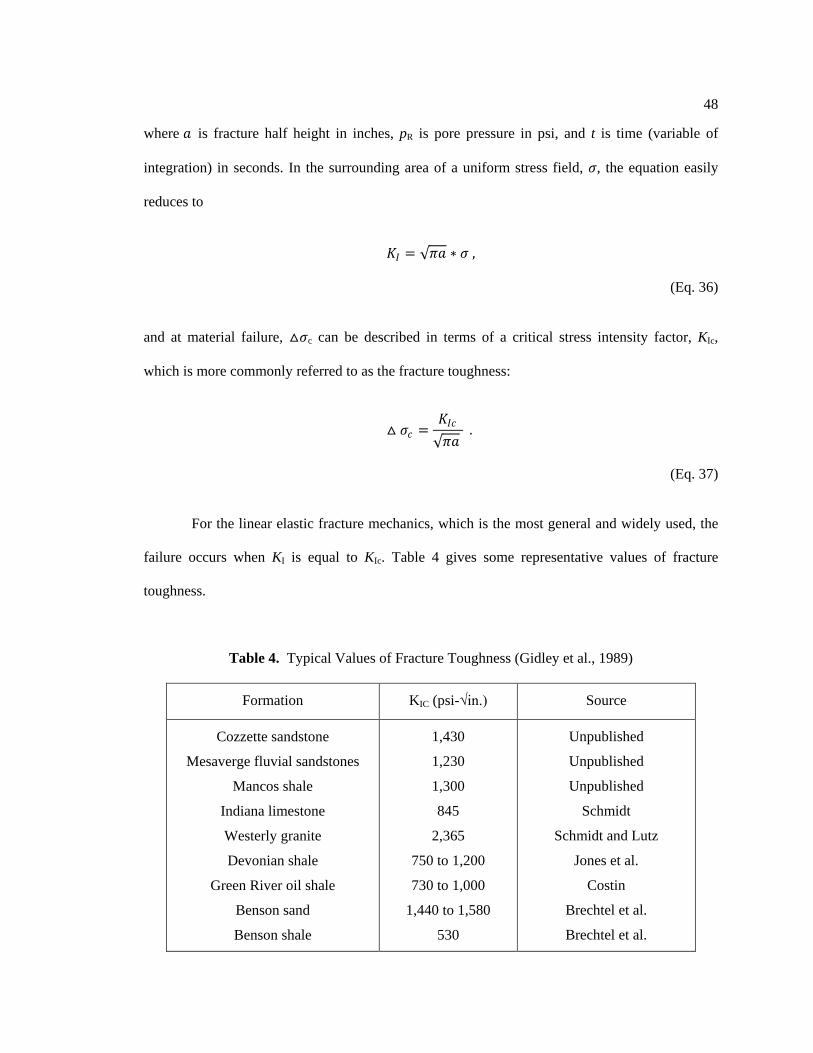
Table 4. Typical Values of Fracture Toughness (Gidley et al., 1989)
Formation KIC (psi-√in.) Source
Cozzette sandstone
Mesaverge fluvial sandstones
Mancos shale
Indiana limestone
Westerly granite
Devonian shale
Green River oil shale
Benson sand
Benson shale
1,430
1,230
1,300
845
2,365
750 to 1,200
730 to 1,000
1,440 to 1,580
530
Unpublished
Unpublished
Unpublished
Schmidt
Schmidt and Lutz
Jones et al.
Costin
Brechtel et al.
Brechtel et al.
49
4.5.2 Applications to Field Data
In this section, rock toughness will be used in the calculation of the net pressure equation.
Therefore, the net pressure formula in Eq. 7 has to be modified to:
𝑝𝑝𝑛𝑛𝑛𝑛𝑛𝑛 = 𝑝𝑝𝑠𝑠𝑠𝑠𝑐𝑐𝑐𝑐 − 𝜎𝜎𝑚𝑚𝑓𝑓𝑛𝑛 −△ 𝜎𝜎𝑐𝑐 .
(Eq. 38)
Using this equation, new values of net pressure will be provided. For the net pressure
calculation, the same field data as given before were applied.
4.5.3 Results and Validations
For case study 1, the critical stress of rock toughness was calculated as 50.1 psi. Case
study 2 produced a pressure value of 25.1 psi as the result. The change in stress due to rock
toughness is a function of stress intensity factor and fracture half height so there was some
difference between the two case studies. The result gives a 25 psi difference between the two
cases because the fracture properties of the two wells are different. One is a sandstone formation
and the other is limestone.

50
4.6 Thermal Effect on In-Situ Stress
When a lower temperature fluid is injected into a higher temperature reservoir, the region
around the injection well will be cooled down. Then a thermoelastic stress field will be induced
around the well because the rock matrix in the cooled region contracts. For typical deep reservoirs,
in-situ stress may be reduced due to this phenomenon.
4.6.1 Thermal Expansion Stress
Changes in the temperature on the casing wall occur when the fracturing fluid is injected,
because the formation is in contact with the fluid at a lower temperature than the formation.
Temperature fluctuates when the injection of fracturing fluid is stopped and resumed. After a
stop, the formation near the well will gradually heat up. Maury and Sauzay (1987) proposed a
study for the delayed failure. As the temperature increases, however, the tangential and vertical
stress at the wellbore will increase by an equal amount:
△ 𝜎𝜎𝑇𝑇 =𝐸𝐸
1 − ν𝛼𝛼𝑇𝑇�𝑇𝑇𝑛𝑛 − 𝑇𝑇𝑠𝑠� ,
(Eq. 39)
where 𝛼𝛼T = thermal expansion coefficient, °C-1,
E = Young’s modulus, GPa,
ν = Poisson’s ratio,
Tt = formation temperature after treatment, °C, and
Tf = original formation temperature, °C.
51
As a matter of fact, thermal expansion coefficients have not been extensively reported.
There is not enough data on thermal expansion, but it is typically around 10-5 °C-1 (Fjaer et al.,
1992). This gives a very low typical thermal stress contribution. The extent of the cold zone may
be limited and this will restrict the fracture growth. If the temperature change occurs, this thermal
effect can become significant.
4.6.2 Applications to Field Data
Inputting the typical thermal expansion coefficient, thermal expansion stress was
calculated by Eq. 39. Young’s modulus and Poison’s ratio were provided by the field data. In the
case of formation temperature, the average geothermal gradient was used by the individual U.S.
state’s data for each well location.
4.6.3 Results and Validations
For typical reservoirs, in-situ stress due to thermal effect would be reduced. The results
show that thermal stresses reduced to 5.121 psi for case study 1 and to 1.351 psi for case study 2.
The reason for the difference between the two cases comes from a difference in well depth as
well as geothermal gradient. Compared with rock toughness, the thermal expansion effect yields a
smaller change.

52
4.7 Effect of Pore Pressure
Pore pressure changes during the treatment due to fracture fluid leak-off. Thus, the
changed pore pressure also causes stress changes in the rock. A study for quantifying the change
of stress was continued by Lubinski (1954). It is assumed that the porosity and permeability are
independent of the stress level so that the change of stress induced by a pressure change can be
calculated in a same way as the change of stress induced by a temperature change.
4.7.1 Pore Pressure Expansion Stress
To quantify the relationship between pore pressure and stress, the linear coefficient of
pore pressure, 𝛼𝛼P, is required. It is defined as the following:
𝛼𝛼𝑃𝑃 =1 − 2ν𝐸𝐸
−𝛽𝛽3
,
(Eq. 40)
where 𝛼𝛼P = pore pressure expansion coefficient, GPa-1,
E = Young’s modulus, GPa,
ν = Poison’s ratio, and
𝛽𝛽 = grain compressibility, kPa-1.
The meaning of 𝛼𝛼P is analogous to the linear thermal expansion coefficient. In the same
way, Perkins and Gonzalez (1985) developed an equation for quantifying pore pressure
expansion. Thus, Eq. 39 can be replaced by
△ 𝜎𝜎𝑃𝑃 =𝐸𝐸
1 − ν𝛼𝛼𝑃𝑃(𝑝𝑝𝑤𝑤𝑤𝑤 − 𝑝𝑝𝑅𝑅) ,
(Eq. 41)
53
where pR is the formation pore pressure in psi. Pore pressure expansion stress, △𝜎𝜎P, can be
explained as the difference between the final and the initial values in the average interior stress
perpendicular to the major axis of the ellipse resulting from a pressure difference between the
elliptical cylinder and the surroundings.
4.7.2 Applications to Field Data
In the same way, pore pressure expansion stress was applied into two case studies. To
obtain the pore pressure expansion coefficient, grain compressibility for each case was
determined by geological data. Note that the unit of grain compressibility is kPa-1, which is
different from the unit of Young’s modulus, so the pore pressure expansion coefficient should be
calculated carefully.
4.7.3 Results and Validations
Finally, we got a 4.149 psi increase in average pore pressure expansion stress for case
study 1 and a 10.85 psi stress increase for case study 2. The difference between the two cases,
results from a difference in the values of bottomhole treating pressure, pore pressure gradient, and
well depth for each location.
Now, we can combine all effects on in-situ stress, such as stress due to rock toughness,
thermal expansion stress, and pore pressure expansion stress. The final equation for in-situ stress
can be:
𝜎𝜎1 = 𝜎𝜎𝑚𝑚𝑓𝑓𝑛𝑛 +△ 𝜎𝜎𝑐𝑐 +△ 𝜎𝜎𝑇𝑇 +△ 𝜎𝜎𝑃𝑃 .
(Eq. 42)
54
where 𝜎𝜎1 is the total opposing earth stress, which is also called in-situ stress briefly. As
mentioned above, 𝜎𝜎min is the minimum in-situ stress, △𝜎𝜎c is the change in stress due to rock
toughness, △𝜎𝜎T is the thermal expansion stress, and △𝜎𝜎P is the pore pressure expansion stress,
respectively.
The result from all effects yields that the total earth stress, 𝜎𝜎1, for case study 1 gives
5,699 psi and 𝜎𝜎1 for case study 2 changes to 5,784 psi. Comparing to the in-situ stresses without
considering those significant factors, 49.1 psi for case 1 and 34.6 psi for case 2 were increased by
new model development.
55
Chapter 5
RESULTS AND ANALYSES
5.1 Interpretation Pressures without Considering All Factors
Case studies of low-permeability gas reservoirs will be applied as examples of calculating
bottomhole treating pressure and interpreting net pressure. Likewise, two sets of field data from
tight gas were donated by Sklar Exploration Company (2008). According to the procedure
introduced in Chapter 3, bottomhole treating pressure is first calculated, then in-situ stress is
identified, and net pressure is finally interpreted. Note that this application is only for cases
without considering all factors described in Chapter 4.
5.1.1 Calculation of Bottomhole Treating Pressure
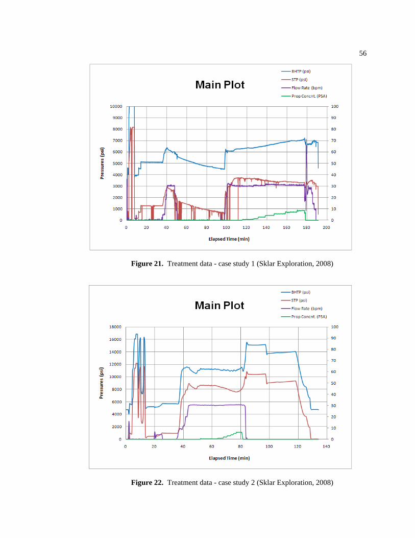
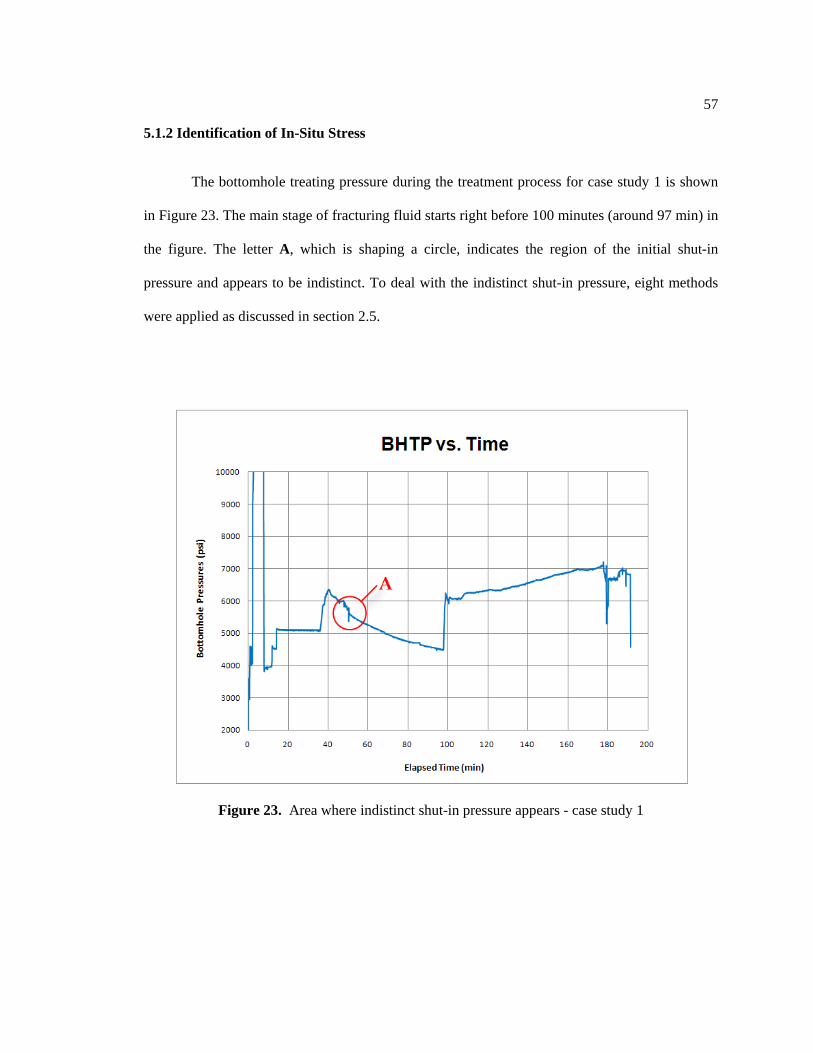
Based on field data given, bottomhole treating pressure was calculated. It is shown as
plots of the pressure vs. elapsed time in Figures 21 and 22. The figures also show surface treating
pressure, fluid flow rate, and proppant concentration for each case.
As seen in both figures, the initial portion of each treatment indicates the formation test
period. The main treatment started at 97 minutes for case 1 and at 35 minutes for case 2. One
important thing to note is that the surface treating pressure starts decreasing during the main
treatment at which proppant concentration increases. This is because an increase in the density of
the fluid causes hydrostatic pressure increase so that the increased hydrostatic pressure leads to a
rise in the bottomhole treating pressure.
56
Figure 21. Treatment data - case study 1 (Sklar Exploration, 2008)
Figure 22. Treatment data - case study 2 (Sklar Exploration, 2008)
57
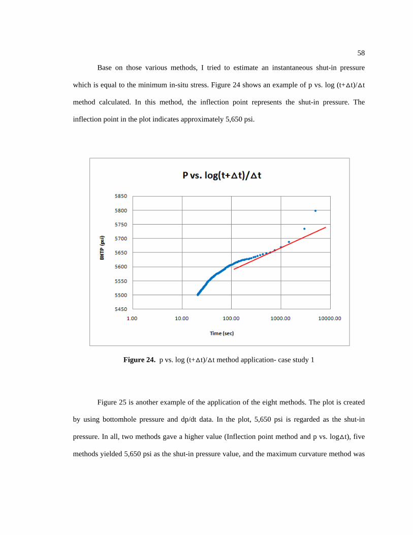
5.1.2 Identification of In-Situ Stress
The bottomhole treating pressure during the treatment process for case study 1 is shown
in Figure 23. The main stage of fracturing fluid starts right before 100 minutes (around 97 min) in
the figure. The letter A, which is shaping a circle, indicates the region of the initial shut-in
pressure and appears to be indistinct. To deal with the indistinct shut-in pressure, eight methods
were applied as discussed in section 2.5.
Figure 23. Area where indistinct shut-in pressure appears - case study 1
58
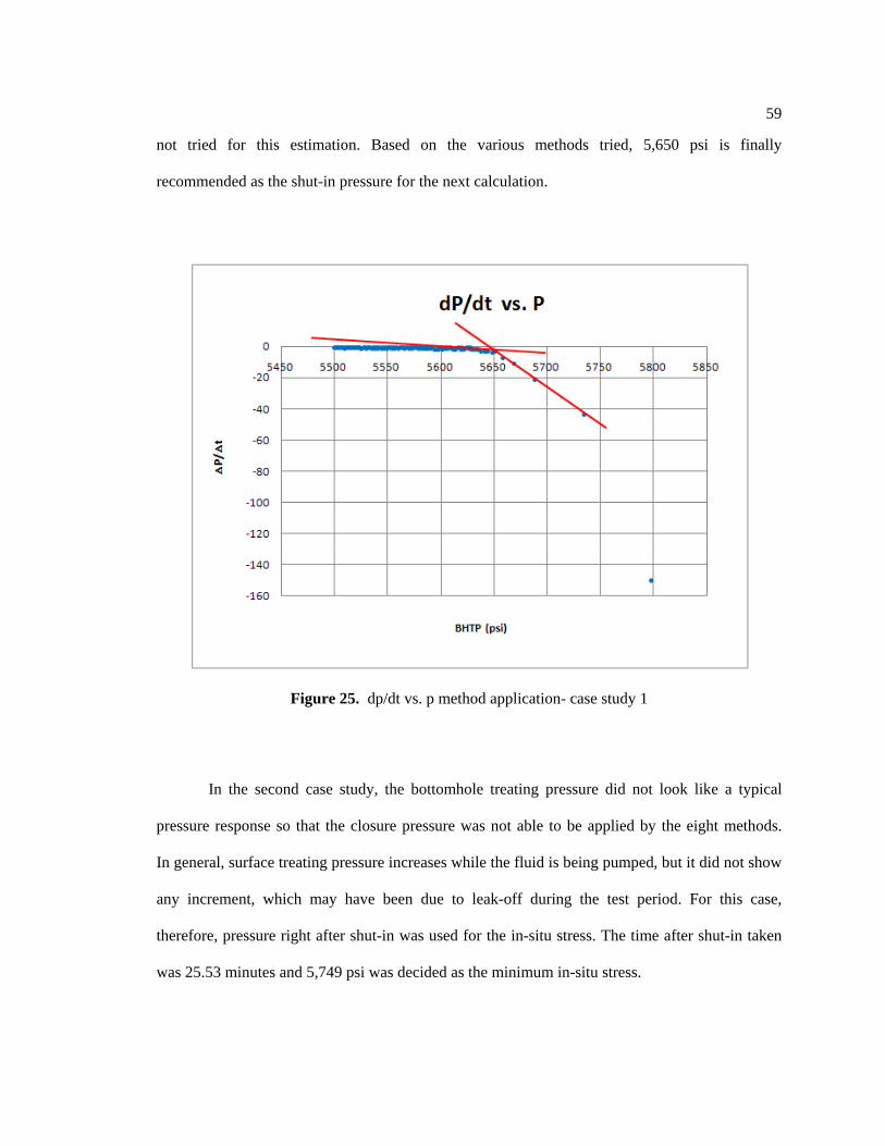
Base on those various methods, I tried to estimate an instantaneous shut-in pressure
which is equal to the minimum in-situ stress. Figure 24 shows an example of p vs. log (t+△t)/△t
method calculated. In this method, the inflection point represents the shut-in pressure. The
inflection point in the plot indicates approximately 5,650 psi.
Figure 24. p vs. log (t+△t)/△t method application- case study 1
Figure 25 is another example of the application of the eight methods. The plot is created
by using bottomhole pressure and dp/dt data. In the plot, 5,650 psi is regarded as the shut-in
pressure. In all, two methods gave a higher value (Inflection point method and p vs. log△t), five
methods yielded 5,650 psi as the shut-in pressure value, and the maximum curvature method was
59
not tried for this estimation. Based on the various methods tried, 5,650 psi is finally
recommended as the shut-in pressure for the next calculation.
Figure 25. dp/dt vs. p method application- case study 1
In the second case study, the bottomhole treating pressure did not look like a typical
pressure response so that the closure pressure was not able to be applied by the eight methods.
In general, surface treating pressure increases while the fluid is being pumped, but it did not show
any increment, which may have been due to leak-off during the test period. For this case,
therefore, pressure right after shut-in was used for the in-situ stress. The time after shut-in taken
was 25.53 minutes and 5,749 psi was decided as the minimum in-situ stress.
60
5.1.3 Interpretation of Fracture Propagation
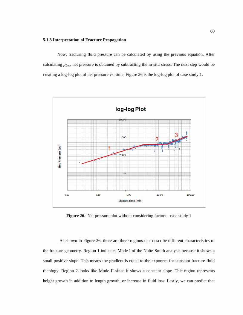
Now, fracturing fluid pressure can be calculated by using the previous equation. After
calculating pfrac, net pressure is obtained by subtracting the in-situ stress. The next step would be
creating a log-log plot of net pressure vs. time. Figure 26 is the log-log plot of case study 1.
Figure 26. Net pressure plot without considering factors - case study 1
As shown in Figure 26, there are three regions that describe different characteristics of
the fracture geometry. Region 1 indicates Mode I of the Nolte-Smith analysis because it shows a
small positive slope. This means the gradient is equal to the exponent for constant fracture fluid
rheology. Region 2 looks like Mode II since it shows a constant slope. This region represents
height growth in addition to length growth, or increase in fluid loss. Lastly, we can predict that

61
region 3 would be Mode III of the Nolte-Smith analysis. This region must be Mode III-a because
the calculated slope is 1.084 and is very close to the unit slope. In this region, we can guess
additional width growth due to a tip screenout process.
Figure 27. Net pressure plot without considering factors - case study 2
On the other hand, case study 2 shows a more complicated shape having five different
regions in Figure 27. This plot also starts with Mode I of the Nolte-Smith analysis. Its exponent
has to be between the time exponent boundaries showing a small positive slope. Region 2 has a
negative slope. According to the Nolte-Smith analysis, it can be represented as rapid height
growth. The next region looks like a unit slope and it indicates Mode III-a. Region 4 shows a
constant gradient and is believed to be because of a confined height or an unrestricted extension.

62
Finally, we can see a steep slope in region 4. This indicates Mode III-b and we can predict a near-
wellbore screenout with a very rapid pressure increase. Lastly, region 6 shows a unique shape
with two different steps, similar to Mode II. We can see that this region displays a pressure
transition after shut-in shown in Figure 22.
In this section, two case studies were applied using basic equations for calculating
bottomhole treating pressure and net pressure. The calculated net pressure for each study was
displayed with a log-log plot. From the log-log plot we predicted fracture geometries based on the
Nolte-Smith analysis. Note that these case studies did not consider some important factors
affecting pressure calculation.
63
5.2 Interpretation of Pressures with New Models
New models were developed and validated with field studies in Chapter 4. This section
rearranges all factors affecting pressure calculation focusing on pressure equations such as the
bottomhole treating pressure equation, hydrostatic pressure equation, fluid friction pressure
equation, perforation friction equation, and in-situ stress calculation. Net pressure in Eq. 7 can be
broken down into the following equations:
𝑝𝑝𝑛𝑛𝑛𝑛𝑛𝑛 = 𝑝𝑝𝑐𝑐𝑠𝑠𝑠𝑠𝑠𝑠 + 𝑝𝑝ℎ𝑦𝑦𝑦𝑦 − 𝑝𝑝𝑠𝑠𝑠𝑠𝑓𝑓𝑐𝑐 −△ 𝑝𝑝𝑝𝑝𝑛𝑛𝑠𝑠𝑠𝑠 − 𝜎𝜎1 .
(Eq. 43)
In the case of surface treating pressure, there is no equation for the calculation since
surface pressure data are measured by the pressure gauge. The rest of the equations were then
checked to see how much each factor influenced the pressure calculations compared to the result
without considering any of the factors.
5.2.1 Changes in Hydrostatic Pressure
A new hydrostatic pressure equation was developed by evaluating the variation of
equivalent static density with temperature and pressure in section 4.1. In this calculation, the
factor affecting the hydrostatic pressure was a change in the fluid density along the wellbore.
As the results of the calculation, hydrostatic pressures after applying the new model
increased such as 54.3 psi for case 1 and 131.7 psi for case 2. Therefore, the pressure increase
results from the increased fluid density.
64
5.2.2 Changes in Fluid Friction Pressure
There are two factors considered to affect fluid friction changes. One is casing roughness
and the other is an additional frictional effect due to proppant. In case of casing roughness,
Fanning friction factor can be the main variable considered because it is a function of casing
roughness. From the new calculation it was concluded that there was no salient change in friction
pressure. The result gave a 0.2 psi increase in case 1 and a 0.9 decrease in case 2. As the other
factor, proppant caused an additional pressure drop of clean fluid. A new correlation for non-
Newtonian fluid was described for calculating the additional friction loss. The result showed
some changes with yielding 24.9 psi for case 1 and 19.5 psi for case 2 as the average pressure
losses.
5.2.3 Changes in Perforation Friction Pressure
As the near-wellbore friction effect, perforation friction pressure and tortuosity pressure
were considered first. However, it is very difficult to make an accurate estimate of tortuosity
pressure so that it will remain as future work. For the calculation of perforation pressure,
coefficient of discharge gradually increased with time compared with the former constant
coefficient. Since the coefficient of discharge is inversely proportional to perforation friction
pressure drop, increase of discharge coefficient caused the perforation pressure to decrease. The
changes of perforation friction pressure for cases 1 and 2 were -58.7 psi and -1.1 psi, respectively.
The difference comes from a greater difference in the perforation number between the two
wellbores.
65
5.2.4 Changes in In-Situ Stress
Three factors affecting the in-situ stress estimation were described in the previous
chapter. First, the critical intensity factor influences in-situ stress. The critical stress of rock
toughness was calculated as 50.1 psi for case 1. Case study 2 yielded 25.1 psi having half the
value of case 1 due to different fracture properties for each well.
The next factor is thermal expansion stress making in-situ stress reduce typically. The
result showed a 5.121 psi decrease for case 1 and a 1.351 psi for case 2. In the same manner, the
last factor, pore pressure expansion stress, affecting in-situ stress was calculated showing a 4.149
psi rise of average stress for case 1 and a 10.85 psi rise of average stress for case 2.
The total opposing earth stress was eventually obtained using Eq. 42 in section 4.7.3.
The calculation yielded a 49.1 psi increase for case 1 and a 34.6 psi increase for case 2.
5.2.5 Interpretation of Fracture Propagation
The final log-log plots of net pressure vs. time for two case studies while considering all
factors are plotted in Figures 28 and 29. The plot of case study 1 displays a slight change in net
pressure. The gradient in region 1 looks gentle compared with the previous gradient, but the net
pressure uniformly increased having the average value of 38.9 psi. The reason why it does not
look uniform from beginning to end is because the plot represents logarithmic scale.
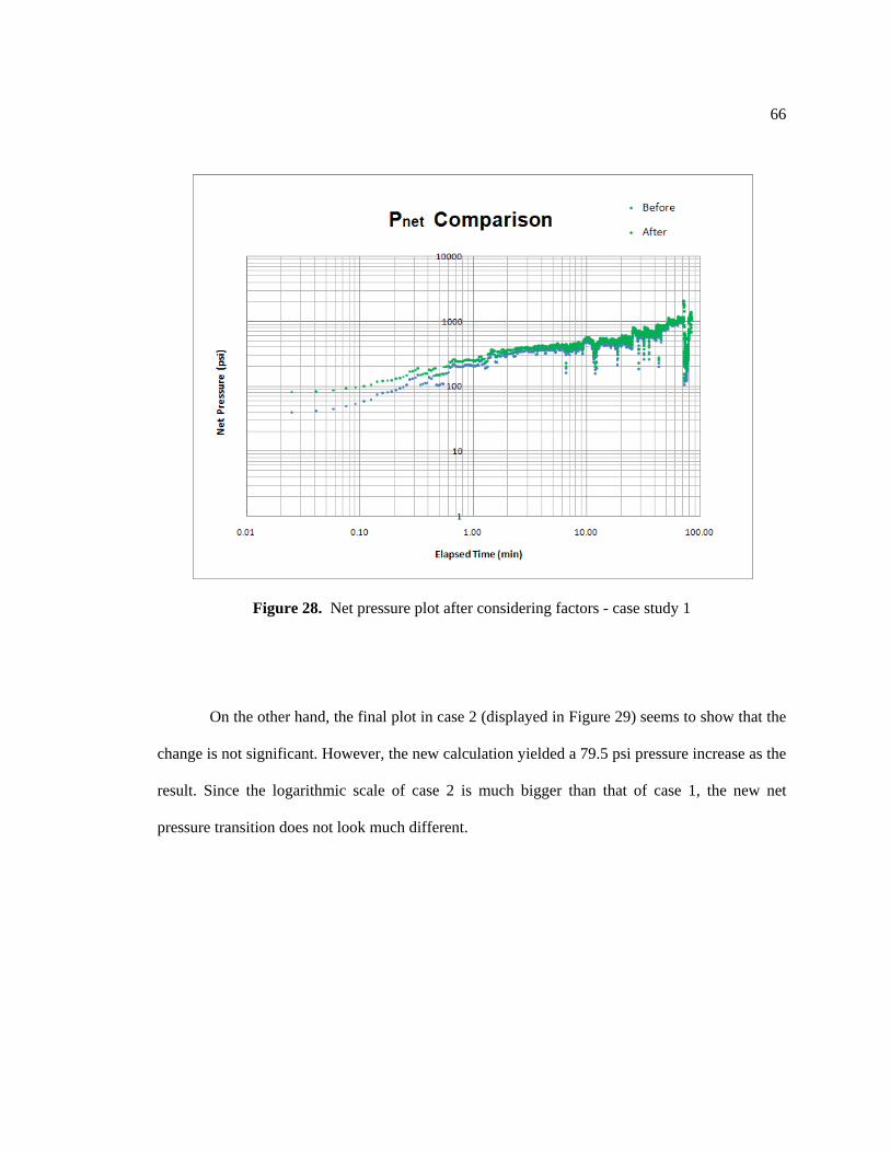
66
Figure 28. Net pressure plot after considering factors - case study 1
On the other hand, the final plot in case 2 (displayed in Figure 29) seems to show that the
change is not significant. However, the new calculation yielded a 79.5 psi pressure increase as the
result. Since the logarithmic scale of case 2 is much bigger than that of case 1, the new net
pressure transition does not look much different.
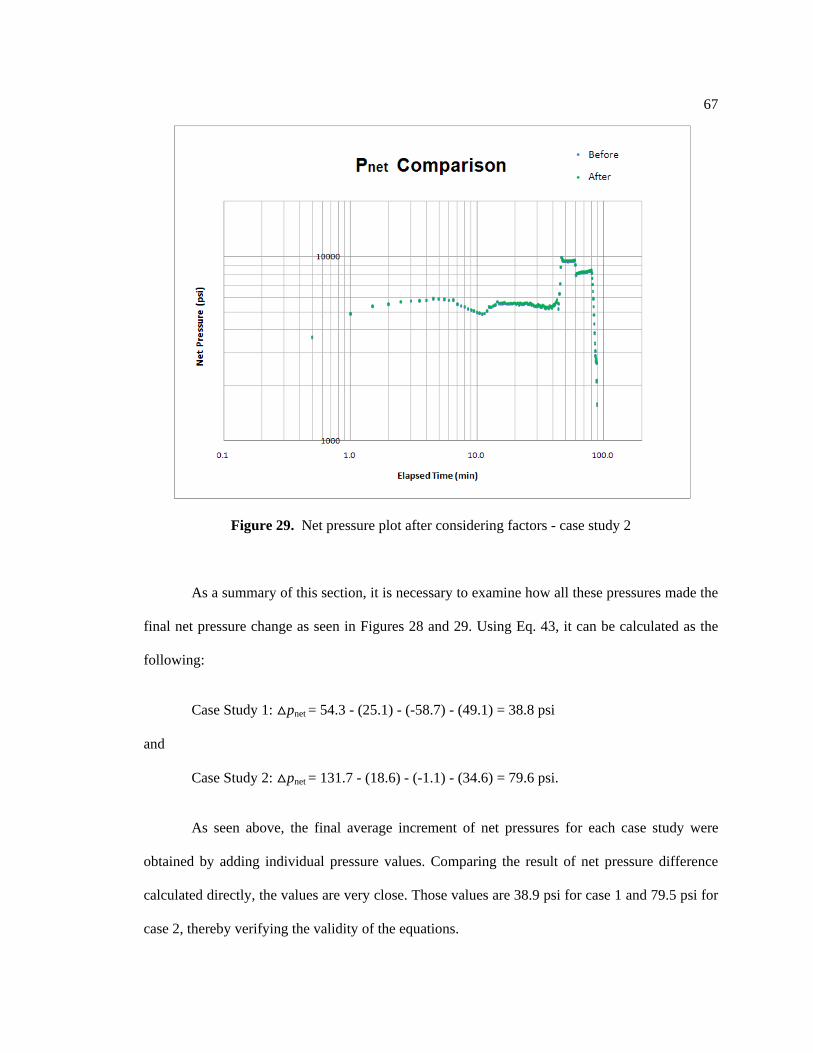
67
Figure 29. Net pressure plot after considering factors - case study 2
As a summary of this section, it is necessary to examine how all these pressures made the
final net pressure change as seen in Figures 28 and 29. Using Eq. 43, it can be calculated as the
following:
Case Study 1: △pnet = 54.3 - (25.1) - (-58.7) - (49.1) = 38.8 psi
and
Case Study 2: △pnet = 131.7 - (18.6) - (-1.1) - (34.6) = 79.6 psi.
As seen above, the final average increment of net pressures for each case study were
obtained by adding individual pressure values. Comparing the result of net pressure difference
calculated directly, the values are very close. Those values are 38.9 psi for case 1 and 79.5 psi for
case 2, thereby verifying the validity of the equations.

68
5.3 New Methods for Interpreting Fracture Geometry
The Nolte-Smith analysis is limited to vertical fractures having a horizontal penetration
where the length of fractures is larger than their vertical height, following the PKN model. In
addition, the analysis assumes that injection rate and fluid viscosity is constant during the fracture
process. However, real field data contain periods of variations of the injection rate and the fluid
viscosity. Thus, a suitable solution for variable injection rate should be considered in order to
apply the result to the Nolte-Smith analysis. In this section, new methods for interpreting fracture
geometry with considering variable flow rate will be introduced by using broad methods.
5.3.1 Fast Fourier Transform (FFT) and Deconvolution Method
The Fourier transform is a mathematical analysis technique which can be used in lots of
engineering fields. FFT is a fast algorithm for evaluating the discrete Fourier transform (DFT),
which can provide exact transformation of a discrete set of data from a digital point of view. The
purpose of this transform is to investigate the frequency signatures of nonperiodic continuous
functions. A nonperiodic function subject is transformed from a time-domain function to a
frequency-domain function. It is important to note that the Fourier integral exists only for a
continuous function. If a set of data cannot be described mathematically as a continuous function,
the integral Fourier transform pair cannot be used (Cheng, 2005).
Deconvolution is a mathematical technique used to convert measured pressure response
from variable-rate well test, or production sequence, into the constant-rate equivalent pressure
response for the entire duration of the test or production history. This method makes the data
more useful for interpretation and allows one to extract more information by using conventional
analysis methods so that it is in turn widely used in many engineering fields (Andrecut, 2009).
69
Based on Duhamel’s principal for conventional well-test analysis, the convolution
integral can be presented as:
𝑝𝑝𝑤𝑤(𝑛𝑛) = � 𝑠𝑠(𝜏𝜏)𝑝𝑝𝛿𝛿(𝑛𝑛 − 𝜏𝜏)𝑦𝑦𝜏𝜏𝑛𝑛
0 ,
(Eq. 44)
where pw is the variable-rate pressure-change response, r is the ratio of time derivative of the
sandface flow rate to a reference rate, and pδ is the constant-rate pressure-change response of the
reservoir. Taking the Fourier transform of Eq. 44 and using the convolution method, we get
𝑝𝑝�𝑤𝑤(𝑠𝑠) = �̃�𝑠(𝑠𝑠) ∗ 𝑝𝑝�𝛿𝛿(𝑠𝑠) ,
(Eq. 45)
where the head ‘~’ means the Fourier transform and 𝑝𝑝�𝛿𝛿 is the constant-rate pressure solution in
the frequency domain. The convolution becomes a multiplication and, thus, deconvolution can be
expressed as:
𝑝𝑝�𝛿𝛿(𝑠𝑠) = 𝑝𝑝�𝑤𝑤(𝑠𝑠)/�̃�𝑠(𝑠𝑠) .
(Eq. 46)
Then, the constant-rate pressure solution in the time domain, pδ, is obtained by the inverse Fourier
transform.
In the field, obtained data are the discrete sets of pressure and injection rate values, so the
convolution and deconvolution expressions in discrete forms are required. The discrete Fourier
transform is defined in the time domain as:
𝑋𝑋𝑦𝑦(𝑘𝑘 △ 𝑠𝑠) =△ 𝑛𝑛 � 𝑥𝑥𝑦𝑦(𝑛𝑛 △ 𝑛𝑛)𝑛𝑛−𝑓𝑓2𝜋𝜋𝑘𝑘△𝑠𝑠𝑛𝑛△𝑛𝑛𝑁𝑁−1
𝑛𝑛=0
.
70
(Eq. 47)
This equation can transform a set of time-domain data to a set of frequency-domain data
inversely. Thus, the inverse discrete Fourier transform can be expressed as:
𝑥𝑥𝑦𝑦(𝑛𝑛 △ 𝑠𝑠) =△ 𝑠𝑠� 𝑋𝑋𝑦𝑦(𝑘𝑘 △ 𝑠𝑠)𝑛𝑛𝑓𝑓2𝜋𝜋𝑘𝑘△𝑠𝑠𝑛𝑛△𝑛𝑛𝑁𝑁−1
𝑘𝑘=0
,
(Eq. 48)
where Xd(k△f) is the set of Fourier coefficients of xd(n△t), which is the set of time data. N is
number of samples, n is the time index (n=0, 1, 2, …, N-1), k is the frequency index (n=0, 1, 2,
…, N-1), △t is the time interval between samples, and △f is the frequency interval. Using this
transform technique and the deconvolution equation, the constant-rate pressure-change response
of the reservoir, pδ, can be calculated. Then, a new log-log plot of net pressure vs. time will be
displayed finally.
5.3.2 Application to Field Data
Some studies have been carried out to find net pressure using the Fourier transform and
the deconvolution techniques during the production process; however, there has been no attempt
to try to find net pressure during the fracturing treatment. New methods for obtaining the net
pressure at the constant flow rate were developed and validated to interpret fracture geometry.
For the calculation of the variable-rate pressure-change response a pressure value at t = 0
was used, where pw = |pw (t=0) – pw (t)|. 30 bbl/min was determined as the reference flow rate for
both cases. Therefore, r would be the ratio of flow rate differential between two adjacent time
points to the reference rate.
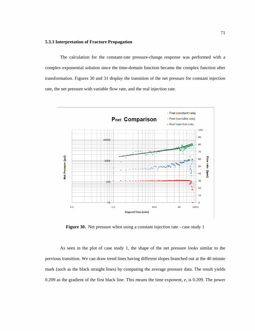
71
5.3.3 Interpretation of Fracture Propagation
The calculation for the constant-rate pressure-change response was performed with a
complex exponential solution since the time-domain function became the complex function after
transformation. Figures 30 and 31 display the transition of the net pressure for constant injection
rate, the net pressure with variable flow rate, and the real injection rate.
Figure 30. Net pressure when using a constant injection rate - case study 1
As seen in the plot of case study 1, the shape of the net pressure looks similar to the
previous transition. We can draw trend lines having different slopes branched out at the 40 minute
mark (such as the black straight lines) by computing the average pressure data. The result yields
0.209 as the gradient of the first black line. This means the time exponent, e, is 0.209. The power
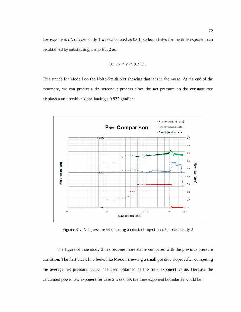
72
law exponent, n’, of case study 1 was calculated as 0.61, so boundaries for the time exponent can
be obtained by substituting it into Eq. 2 as:
0.155 < 𝑛𝑛 < 0.237 .
This stands for Mode I on the Nolte-Smith plot showing that it is in the range. At the end of the
treatment, we can predict a tip screenout process since the net pressure on the constant rate
displays a unit positive slope having a 0.925 gradient.
Figure 31. Net pressure when using a constant injection rate - case study 2
The figure of case study 2 has become more stable compared with the previous pressure
transition. The first black line looks like Mode I showing a small positive slope. After computing
the average net pressure, 0.173 has been obtained as the time exponent value. Because the
calculated power law exponent for case 2 was 0.69, the time exponent boundaries would be:
73
0.148 < 𝑛𝑛 < 0.228 .
The gradient of case 2 is also in the range of the exponent boundaries so that the process would
be in Mode I. In addition, the second black line shows a steep positive slope having a 1.802
gradient. It means that there might be a screenout near the wellbore. The rest of the plot displays a
small negative slope, so we can predict an unstable height growth.

74
Chapter 6
CONCLUSIONS AND RECOMMENDATIONS
A new model for the accurate calculation of hydraulic fracturing pressure has been
developed and validated with field data from tight gas and shale gas reservoirs. This new model
will serve as a valuable reference for the analysis of pressure response from a formation during
the fracturing process. The following conclusions were summarized from this research:
• Factors studied in this research are important to interpret fracture geometry and formation
properties.
• Density and perforation friction have significantly influenced the calculation of
bottomhole treating pressure, while the other factors have made small changes in the
calculation.
• Rock toughness was the main factor affecting in-situ stress change compared with
thermal and pore pressure expansion effects.
• The net pressure after considering all factors changed slightly and it was verified by the
validity of the equations.
• New methods for fracture diagnostics have been described to interpret fracture geometry
by using the Fast Fourier Transforms (FFT) and the deconvolution techniques.
• A new log-log plot for constant-rate pressure-change response has been demonstrated and
analyzed with the same field data.
• The result after using the new methods showed clearer and more stable pressure
transitions compared with the previous transitions.
75
There are more factors that I will study to improve the pressure calculation in the future.
Factors such as near-wellbore tortuosity certainly affect frictional pressure change. Even though it
is very difficult to quantify tortuosity, this pressure loss should be given more weight than
perforation friction pressure at the beginning of the fracture treatment. In addition, the effect of
multiphase flow on pressure response should be included as well. Once a complete model is
developed for vertical wells, the model can be extended to horizontal wells with multistage
fracture treatments.

76
NOMENCLATURE
a fracture half height [in]
A kinetic energy constant [ - ]
B kinetic energy exponent [ - ]
C0~5 empirical constants for oil density [ - ]
D0~2 empirical constants for water density [ - ]
Cd coefficient of discharge [ - ]
Cυ frictional volumetric concentration of proppant [ - ]
d pipe diameter [in]
Dp perforation diameter [in]
e time exponent [ - ]
E Young’s modulus [GPa]
f Fanning friction factor [ - ]
fo, fw volume fractions of oil and water [ - ]
g gravitational acceleration [ft/sec2]
h well depth [ft]
KI stress intensity factor [psi-√in]
KIc critical stress intensity factor [psi-√in]
K’ consistency index [lb-secn’/ft2]
L length of pipe [ft]
n’ flow behavior index [ - ]
Np perforation number [ - ]
NRe Reynolds number [ - ]

77
pfrac fracturing fluid pressure [psi]
pfric fluid friction pressure [psi]
phyd hydrostatic pressure [psi]
pnet Net pressure [psi]
psurf surface treating pressure [psi]
pw variable-rate pressure-change response [psi]
pwb bottomhole treating pressure [psi]
pR formation pore pressure [psi]
pδ constant-rate pressure-change response [psi]
△pclean fluid friction pressure of clean fluid [psi]
△pD dimensionless pressure drop parameter [ - ]
△pnet net pressure difference [psi]
△pperf perforation friction pressure [psi]
△pprop additional pressure drop due to proppant [psi]
q fluid flow rate [bpm]
r time derivative of sandface rate/reference rate [ - ]
r2 correlation coefficient [ - ]
t pumping time [min or sec]
△t time since shut-in [sec]
T wellbore temperature [°C]
Tf original formation temperature [°C]
Tt Formation temperature after treatment [°C]
𝜌𝜌 fluid velocity [ft/sec]
𝜌𝜌t single particle-settling velocity [ft/sec]
�̅�𝜌 mean suspension velocity [ft/sec]
78
�̅�𝜌s mean slip velocity [ft/sec]
𝛼𝛼P pore pressure expansion coefficient [GPa-1]
𝛼𝛼T thermal expansion coefficient [°C-1]
𝛽𝛽 grain compressibility [kPa-1]
ε absolute roughness [in]
θ dial reading of rotational viscometer [ - ]
𝑑𝑑 fluid viscosity [cp]
𝑑𝑑a apparent viscosity [cp]
ν Poisson’s ratio [ - ]
Π dimensionless group [ - ]
𝜌𝜌 fluid density [lb/gal]
𝜌𝜌m1 mud density at reference conditions [lb/gal]
𝜌𝜌m2 mud density at elevated conditions [lb/gal]
𝜌𝜌p particle density [lb/gal]
𝜌𝜌s slurry density [lb/gal]
𝜌𝜌o1, 𝜌𝜌w1 oil and water density at reference conditions [lb/gal]
𝜌𝜌o2, 𝜌𝜌w2 oil and water density at elevated conditions [lb/gal]
△𝜌𝜌 slurry density – clean fluid density [lb/gal]
𝜎𝜎 uniform stress [psi]
𝜎𝜎1 earth stress or in-situ stress [psi]
𝜎𝜎min minimum in-situ stress [psi]
△𝜎𝜎c change in stress due to rock toughness [psi]
△𝜎𝜎P pore pressure expansion stress [psi]
△𝜎𝜎T thermal expansion stress [psi]
79
REFERENCES
Amadei, B. and Stephansson, O.: “Rock Stress and its Measurement,” Chapman and Hall; 1st
edition, January 1997.
Aggson, J. R. and Kim, K.: “Technical Note-Analysis of Hydraulic Fracturing Pressure Histories:
A Comparison of Five Methods Used to Identify Shut-In Pressure,” Int. J. Rock Mech. Min. Sci.
& Geomech. Abstr. Vol. 24, 75-80, 1987.
Andrecut, M.: “Pressure Rate Deconvolution Methods for Well Test Analysis,” Modern Physics
Letters B, Vol. 23 (8), June 2009.
Bourgoyne, A. T., Millheim, K. K., Chenevert, M. E., and Young, F. S.: “Applied Drilling
Engineering,” Society of Petroleum Engineers, SPE Textbook Series Vol. 2, Richardson, TX,
1986.
Cheng, Y., Lee, W. J., and McVay, D. A.: “Fast-Fourier-Transform-Based Deconvolution for
Interpretation of Pressure-Transient-Test Data Dominated by Wellbore Storage,” SPE 84471,
SPE Reservoir Evaluation & Engineering Vol. 8 (3), June 2005.
Cleary, J. M.: “Hydraulic Fracturing Theory, Part I - Mechanics of Materials,” Illinoise State
Geological Survey, Urbana, IL, 1958.
Colebrook, C. F.: “Turbulent Flow in Pipes, with Particular Reference to the Transition Region
Between the Smooth and Rough Pipe Laws,” J. Inst. Civil Engs., London, February 1939.
Crump, J. B. and Conway, M. W.: “Effect of Perforation-Entry Friction on Bottomhole Treating
Analysis,” SPE 15474, J. Petr. Tech. Vol. 40 (8), 1041-1048, August 1988.
Dodge, D. G. and Metzner, A. B.: “Turbulent Flow of Non-Newtonian Systems,” AIChE J. Vol. 5
(2), 189-204, June 1959.
DOE/EIA report: “Annual Energy Outlook 2010 with Projections to 2035: Importance of low-
permeability natural gas reservoir,” EIA, http://www.eia.doe.gov/oiaf/aeo/lpnat_gas.html, 2010.
80
Economides, M. J. and Martin, T.: “Modern Fracturing-Enhancing Natural Gas Production,” ET
Publishing, Houston, TX, 2007.
Economides, M. J. and Nolte, K. G.: “Reservoir Stimulation, Second edition,” Prentice-Hall, Inc.,
Englewood Cliffs, NJ, March 1991.
El-Rabba, A. M., Shah, S. N., and Lord, D. L.: “New Perforation Pressure-Loss Correlations for
Limited-Entry Fracturing Treatments,” SPE 54533, SPE Prod. & Facilities Vol. 14 (1), February
1999.
Fjaer, E., Holt, R. M., Horsrud, P., Raaen, A. M., and Risnes, R.: “Petroleum Related Rock
Mechanics,” Elsevier, Amsterdam, 1992.
Gidley, J. L., Holditch, S. A., Nierode, D. E., and Veatch, R. W.: “Recent Advances in Hydraulic
Fracturing,” Society of Petroleum Engineers, Richardson, TX, 1989.
Gonzalez, T. K. Perkins and J.A.: “The Effect of Thermoelastic Stresses on Injection Well
Fracturing,” SPE 11332, SPE Journal Vol. 25 (1), February 1985.
Guo, F., Morgenstern, N. R., and Scott, J. D.: “Technical Note- Interpretation of Hydraulic
Fracturing Pressrue: A Comparison of Eight Methods Used to Identify Shut-In Pressure,” Int. J.
Rock Mech. Min. Sci. & Geomech. Abstr. Vol. 30, 627-631, 1993.
Harris, O. O. and Osisanya, S. O.: “Evaluation of Equivalent Circulating Density of Drilling
Fluids Under High-Pressure/High Temperature Conditions,” SPE 97018, SPE Annual Technical
Conference and Exhibition, Dallas, TX, October 2005.
Hoberock, L. L., Thomas, D. C., and Nickens, H. V.: “Here’s How Compressibility and
Temperature Affect Bottom-Hole Mud Pressure,” OGJ Vol. 80 (12), 22 March 1982.
Irwin, G. R.: “Analysis of Stresses and Strains Near the End of a Crack Traversing a Plate,” J.
App. Meth., Vol. 24, 361-364, 1957.
Kehle, R.O.: “The Determination of Tectonic Stresses through Analysis of Hydraulic Well
Fracturing,” J. Geophys. Res. Vol. 69 (2), 259-273, 1964.
81
Lubinski, A.: “Theory of Elasticity for porous Bodies Displaying a Strong Pore Structure,” Proc.,
Second U.S. Natl. Cong. Appl. Mech., 1954.
Maury, V.M. and Sauzay, J.M.: “Borehole Instability: Case Histories, Rock Mechanics Approach
and Results,” SPE 16051, SPE/IADC Drilling Conference, New Orleans, LA, March 1987.
Molerus, O. and Wellmann, P.: “A New Concept for the Calculation of Pressure Drop with
Hydraulic Transport of Solids in Horizontal Pipes,” Chem. Eng. Sci. Vol. 36 (10), 1623-1632,
February 1981.
Nolte, K. G.: “Application of Fracture Design Based on Pressure Analysis,” SPE 13393, SPE
Production Eng. Vol.3 (1), 31-42, February 1988.
Nolte, K. G.: “Fracturing-Pressure Analysis for Nonideal Behavior,” SPE 20704, J. Petr. Tech.
Vol. 43, 210-218, February 1991.
Nolte, K.G.: “Principles for fracture design based on pressure analysis,” SPE 10911, SPE
Production Eng. Vol. 3 (1), 22-30, February 1988.
Nolte, K. G. and Smith, M. B.: “Interpretation of Fracturing Pressures,” SPE 8297, J. Petr. Tech.
Vol. 33, 1767-1775, September 1981.
Pepin, G., Gonzalez, M, Bloys, J. B., Lofton, J., Schmidt, J., Naquin, C., and Ellis, S.: “Effect of
Drilling Fluid Temperature on Fracture Gradient: Field Measurements and Model Predictions,”
American Rock Mech. Association, Gulf Rocks 2004, the 6th North America Rock Mechanics
Symposium (NARMS), Houston, TX, June 2004.
Pollitte, M. D.: “Invert Oil Mud Rheology as a Function of Temperature and Pressure,” SPE
13458, SPE/IADC Drilling Conference, New Orleans, LA, 5-8 March 1985.
Rice, J. R.: “Mathematical Analysis in the Mechanics of Fracture,” Fracture, H. Liebowitz ed.,
Academic Press, New York City,NY, 191-311, 1968.
Romero, J., Mack, M. G., and Elbel, J. L.: “Theoretical Model and Numerical Investigation of
Near-Wellbore Effects in Hydraulic Fracturing,” SPE 30506, SPE Annual Technical Conference
and Exhibition, Dallas, TX, October 1995.

82
Shah, S. N. and Asadi, M: “Fracturing Fluid Characterization: State-of-the-Art Facility and
Advanced Technology,” DE-FC21-92MC29077, U.S. Department of Energy Vol. 14 (1),
February 2000.
Shah, S. N. and Lee, Y. N.: “Friction Pressures of Proppant-Laden Hydraulic Fracturing Fluids,”
SPE 13836, SPE Production Engineering Vol. 1 (6), November 1986
Sorelle, R. R., Jardiolin, R. A., Buckley, P., and Barios, J. R.: “Mathematical Field Model
Predicts Down-hole Density Changes in Static Drilling Fluids,” SPE 11118, SPE Annual
Technical Conference and Exhibition, New Orleans, LA, 26-29 September 1982.
Tunbridge, L. W.: “Technical Note-Interpretation of the Shut-In Pressure from the Rate of
Pressure Decay,” Int. J. Rock Mech. Min. Sci. & Geomech. Abstr. Vol. 26, 457-459, 1989.
Willingham, J. D., Tan, H. C., and Norman, L. R.: “Perforation Friction Pressure of Fracturing
Fluid Slurries,” SPE 25891, Low Permeability Reservoirs Symposium, Denver, CO, 26-28 April
1993.
Wright, C. A., Tanigawa, J. J., Mei, S., and Li, Z.: “Enhanced Hydraulic Fracture Technology for
a Coal Seam Reservoir in Central China,” SPE 29989, International Meeting on Petroleum
Engineering, Beijing, China, November 1995.
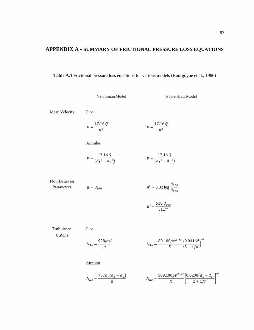
83
APPENDIX A - SUMMARY OF FRICTIONAL PRESSURE LOSS EQUATIONS
Table A.1 Frictional pressure loss equations for various models (Bourgoyne et al., 1986)
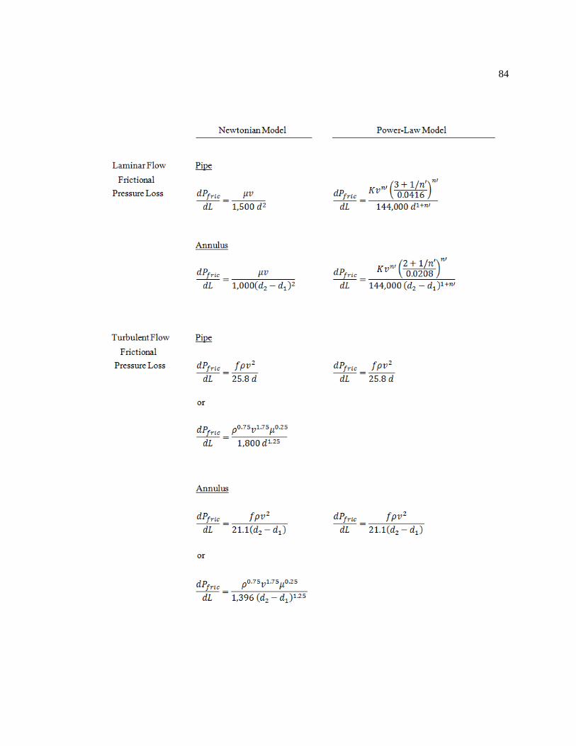
84
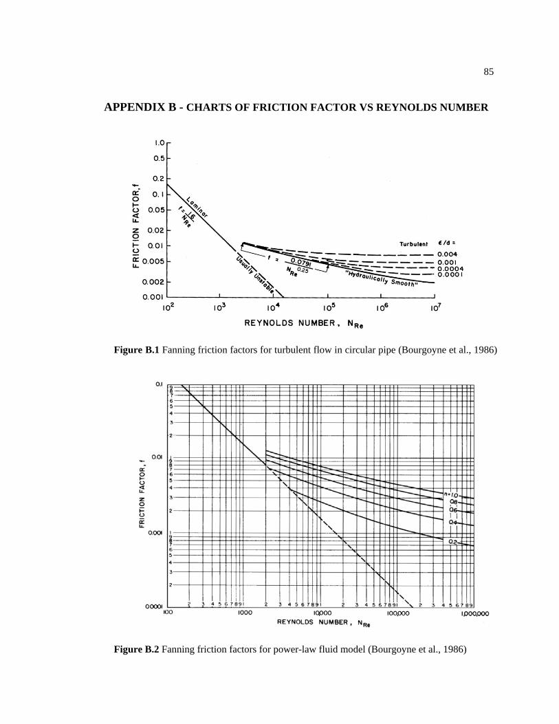
85
APPENDIX B - CHARTS OF FRICTION FACTOR VS REYNOLDS NUMBER
Figure B.1 Fanning friction factors for turbulent flow in circular pipe (Bourgoyne et al., 1986)
Figure B.2 Fanning friction factors for power-law fluid model (Bourgoyne et al., 1986)
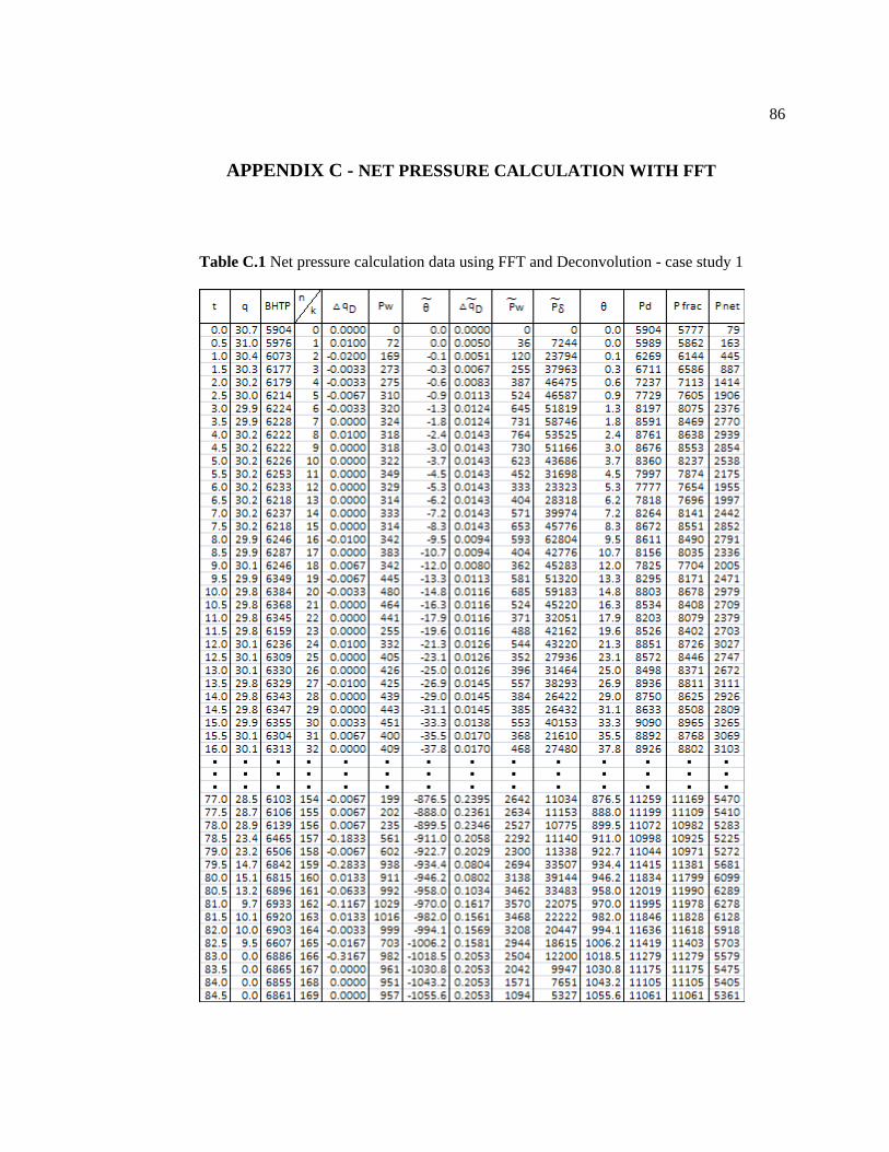
86
APPENDIX C - NET PRESSURE CALCULATION WITH FFT
Table C.1 Net pressure calculation data using FFT and Deconvolution - case study 1
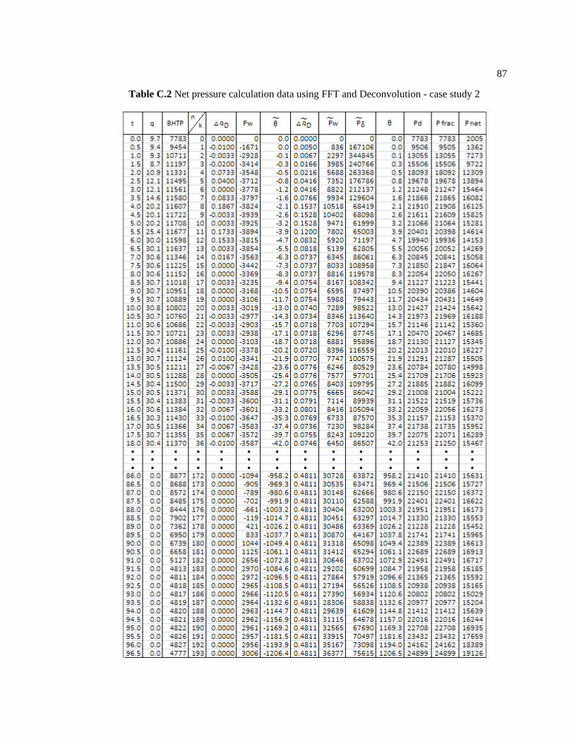
87
Table C.2 Net pressure calculation data using FFT and Deconvolution - case study 2