Interpreting 2D ModelsWhen is a Model Right and

When is it Wrong?

FMA Conference, Sacramento, USA, 2012

Bill SymePhillip Ryan

2

Full 1D Equations (St Venant)

Mass Balance

Momentum0 =u |u| k + xhg +

xuu +

tu

0 = xW

(uA)th

0 = y

(Hv) + x

(Hu) + th

Mass Balance

Momentum

Full 2D Equations (SWE)

New terms introduced – cross momentum, sub-grid scale turbulence

F = xp

yu +

xu -

HCv + uu g +

xh g + v c - y

u v + xuu +

tu

x2

2

2

2

2

22

f

1

3

Inside the Fully 2D Cell

2D equations include effect of cross-momentum, eddy viscosity

4

Inside the Fully 2D Cell

1D equations exclude these influences

5

The Assumptions – 1D Depth and width averaged

Water surface is horizontal

Flow follows a straight line

Most model momentum (in a straight line)

No cross-momentum

No turbulence (eddy viscosity)

Examples: HEC-RAS, MIKE 11, XP-SWMM, TUFLOW 1D

6

The Assumptions – Pseudo-2D Depth averaged

Solves 1D equation over 2D grid/mesh

Spreading model

Diminished or no cross momentum

No turbulence

Simplistic representation of true 2D solution

Can be used where friction dominates (eg. shallow flow)

Velocity output not reliable

Example: FLO-2D

7

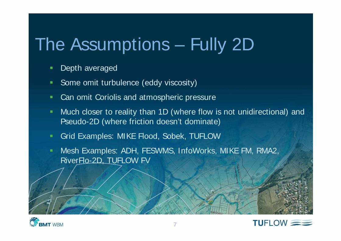
The Assumptions – Fully 2D Depth averaged

Some omit turbulence (eddy viscosity)

Can omit Coriolis and atmospheric pressure

Much closer to reality than 1D (where flow is not unidirectional) and Pseudo-2D (where friction doesn’t dominate)

Grid Examples: MIKE Flood, Sobek, TUFLOW

Mesh Examples: ADH, FESWMS, InfoWorks, MIKE FM, RMA2, RiverFlo-2D, TUFLOW FV

8

Full 2D Equations(Wave length much larger than depth, eg. floods)

Inertia Term

How Velocitychanges over time

CoriolisForce

GravityBed

ResistanceViscosity

(Turbulence)

AtmosphericPressure

ExternalForces(Wind,

Waves, …)

F =yp

yv +

xv -

Hv + u nv g +

yh g +u c +

yv v +

xvu +

tv

y2

2

2

222

f

1

34

2

9

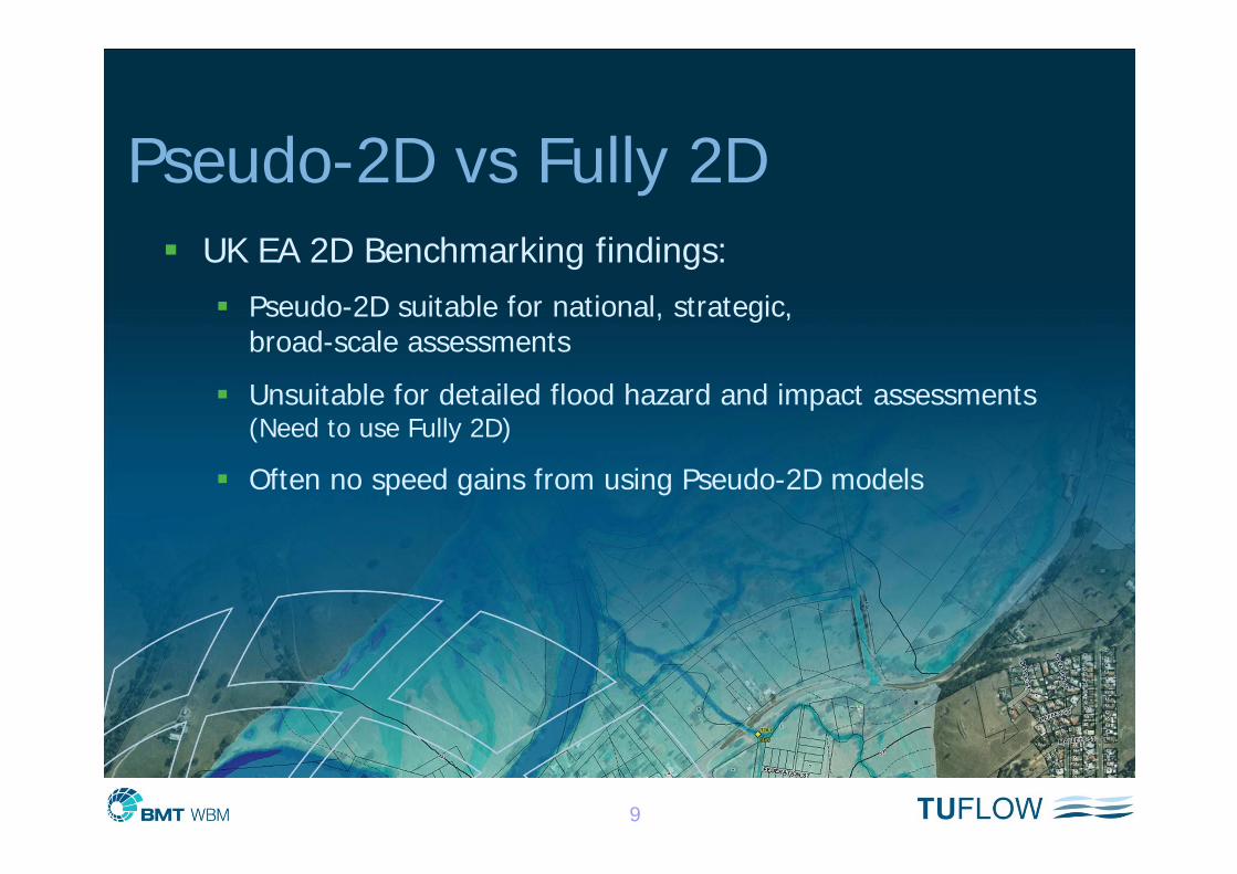
Pseudo-2D vs Fully 2D UK EA 2D Benchmarking findings:

Pseudo-2D suitable for national, strategic, broad-scale assessments

Unsuitable for detailed flood hazard and impact assessments(Need to use Fully 2D)

Often no speed gains from using Pseudo-2D models

10

Accuracy Example

Fully 2D Solutions

Pseudo-2D

11

Key Physical Processes

Inertia Term

How Velocitychanges over time

CoriolisForce

GravityBed

ResistanceViscosity

(Turbulence)

AtmosphericPressure

ExternalForces(Wind,

Waves, …)

Understand what your 2D scheme needs to solve?

F =yp

yv +

xv -

Hv + u nv g +

yh g +u c +

yv v +

xvu +

tv

y2

2

2

222

f

1

34

2

12

2D Grid or Flexible Mesh? Principal Grid Applications

Flood studies

Flood impact assessments

Floodplain management what-if scenarios

Whole of catchment modelling

Principal Flexible Mesh Applications

Detailed, high resolution, analyses (eg. hydraulic structures)

Complex in-bank river flow patterns

Storm surge estuarine and coastal inundation

13

Grid Pros and Cons Pros

Very quick to setup

Mesh remains unchanged (ie. base case results don’t change)

Usually fixed timestep (good for flood impact assessments)

Faster (for same number of elements)

Cons

Resolution too coarse in key areas (hydraulics not well resolved)

Resolution too fine (excessive amount of elements – long run times)

Thus far, vast majority 2D flood models in Australia and UK grid based

14

Flexible Mesh Pros and Cons Pros

Element size reflects resolution needed to resolve hydraulics

Number of elements optimised to reduce run times

Cons Longer setup times and mesh refinement

Timestep reduced by very small elements

Changing mesh for what-if scenarios can change base case results(issue for BFE’s and flood impact assessments)

15

2D Element Size(Mesh Convergence)

Cell/Element Size(s)

Small enough to meet hydraulic objectives

Large enough to minimise run-times

Coarser than DEM

For a fixed grid model halving the cell size increases run-times by a factor of eight (8) – keep this in mind!

16

BreachBreachBreachBreachBreachBreachBreachBreachBreach

20m Cells20m Cells20m Cells20m Cells20m Cells20m Cells20m Cells20m Cells20m CellsBreachBreachBreachBreachBreachBreachBreachBreachBreach

17

10m Cells10m Cells10m Cells10m Cells10m Cells10m Cells10m Cells10m Cells10m CellsBreachBreachBreachBreachBreachBreachBreachBreachBreach

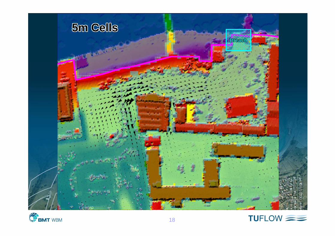
18

5m Cells 5m Cells 5m Cells 5m Cells 5m Cells 5m Cells 5m Cells 5m Cells 5m CellsBreachBreachBreachBreachBreachBreachBreachBreachBreach

19

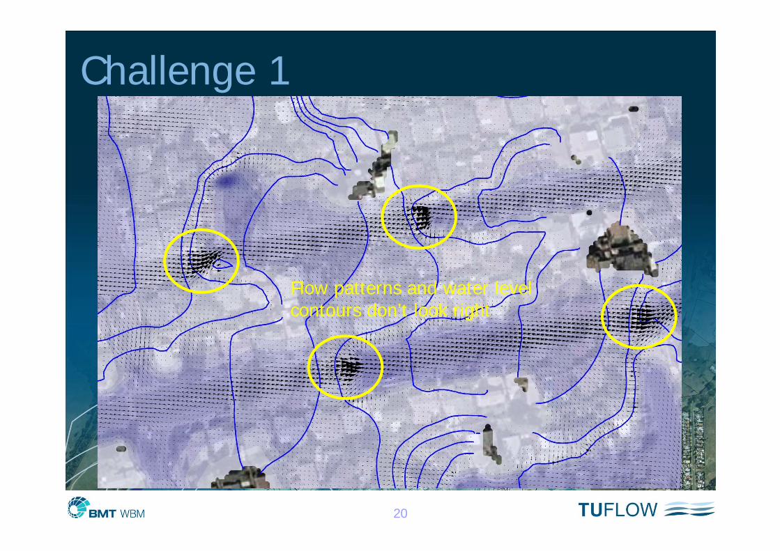
Proofing a Model Look at the results!

Velocities / flow patterns

Water levels

Energy always reduces downstream

20

Challenge 1

Flow patterns and water level contours don’t look right

21

Challenge 1

Look at the model topography

22

Challenge 1

23

Mass Error – Solution Convergence Less than 1% a good benchmark for adequate convergence

2010 UK EA 2D Benchmarking: “The largest volume change reported is a 1.4% volume loss. This did not have any identifiable consequence in the results, and the effect of model choice was clearly more significant than a lack of volume conservation of this magnitude.”

24

Acceptable n ValuesAre Manning’s n Values the same for 1D and 2D models?

Generally, Manning’s n values are usually very similar for 1D and 2D schemes, except:

Rapid changes in flow direction and magnitude (eg. at a structure, sharp bend or embankment opening)

Fully 2D schemes simulate energy losses associated with water changing flow direction and magnitude(may need some minor additional energy loss for fine-scale and/or 3D effects)

1D schemes require: (a) a structure with energy losses; (b) artificially high Manning’s n; or (c) an additional energy loss

2D schemes typically apply no side wall friction Where there is significant wall friction a 2D scheme may require a slightly higher

Manning’s n than a 1D scheme

25

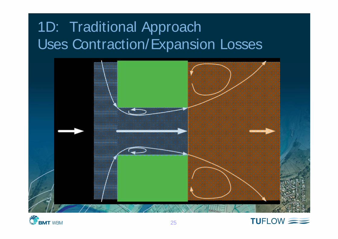
1D: Traditional ApproachUses Contraction/Expansion Losses

26

2D: No Contraction/Expansion Losses?

27

Water Surface Profiles - Outlet Controlled

2.2

2.3

2.4

2.5

2.6

2.7

2.8

2.9

3

0 50 100 150 200 250 300Distance (m)

Wat

er L

evel

(m)

1D Model

Upstreamof Culvert

Downstreamof Culvert

1 1 2 3 4 2 3 0.7 m/s0.7 m/s0.7 m/s0.7 m/s0.7 m/s0.7 m/s0.7 m/s0.7 m/s0.7 m/s 2.9 m/s2.9 m/s2.9 m/s2.9 m/s2.9 m/s2.9 m/s2.9 m/s2.9 m/s2.9 m/s 0.8 m/s0.8 m/s0.8 m/s0.8 m/s0.8 m/s0.8 m/s0.8 m/s0.8 m/s0.8 m/s

2.42 m2.42 m2.42 m2.42 m2.42 m2.42 m2.42 m2.42 m2.42 m2.86 m2.86 m2.86 m2.86 m2.86 m2.86 m2.86 m2.86 m2.86 m2.88 m2.88 m2.88 m2.88 m2.88 m2.88 m2.88 m2.88 m2.88 m 2.30 m2.30 m2.30 m2.30 m2.30 m2.30 m2.30 m2.30 m2.30 m

28

Water Surface Profiles - Outlet Controlled

2.2

2.3

2.4

2.5

2.6

2.7

2.8

2.9

3

0 50 100 150 200 250 300Distance (m)

Wat

er L

evel

(m)

1D Model

2D Model (Culvert as 2D Cells)

Upstreamof Culvert

Downstreamof Culvert

Modify 2D Cells to represent culvert

Water Surface Profiles - Outlet Controlled

2.2

2.3

2.4

2.5

2.6

2.7

2.8

2.9

3

0 50 100 150 200 250 300Distance (m)

Wat

er L

evel

(m)

1D Model

2D Model (Culvert as 2D Cells)

Upstreamof Culvert

Downstreamof Culvert

“Calibrating” 2D Structures

For example, adding 0.2 energy loss, ie. add 0.2*V2/2gcompensates for energy losses not modeled

Water Surface Profiles - Outlet Controlled - Adjusted Form Losses

2.2

2.3

2.4

2.5

2.6

2.7

2.8

2.9

3

0 50 100 150 200 250 300Distance (m)

Wat

er L

evel

(m)

1D Model

2D Model (Culvert as 2D Cells)

Upstreamof Culvert

Downstreamof Culvert

FMA Conference, Sacramento USA

30

1D/2D Link Options

Water Surface Profiles - Outlet Controlled

2.2

2.3

2.4

2.5

2.6

2.7

2.8

2.9

3

0 50 100 150 200 250 300Distance (m)

Wat

er L

evel

(m)

1D Model

Upstreamof Culvert

Downstreamof Culvert

Water Surface Profiles - Outlet Controlled

2.2

2.3

2.4

2.5

2.6

2.7

2.8

2.9

3

0 50 100 150 200 250 300Distance (m)

Wat

er L

evel

(m)

1D Model

2D Model (Culvert as 2D Cells)

Upstreamof Culvert

Downstreamof Culvert

Water Surface Profiles - Outlet Controlled

2.2

2.3

2.4

2.5

2.6

2.7

2.8

2.9

3

0 50 100 150 200 250 300Distance (m)

Wat

er L

evel

(m)

1D Model

2D Model (Culvert as 2D Cells)

2D Model (Culvert as 1D Element)

Upstreamof Culvert

Downstreamof Culvert

1 1 2 3 4 2 3 0.7 m/s0.7 m/s0.7 m/s0.7 m/s0.7 m/s0.7 m/s0.7 m/s0.7 m/s0.7 m/s 2.9 m/s2.9 m/s2.9 m/s2.9 m/s2.9 m/s2.9 m/s2.9 m/s2.9 m/s2.9 m/s 0.8 m/s0.8 m/s0.8 m/s0.8 m/s0.8 m/s0.8 m/s0.8 m/s0.8 m/s0.8 m/s

2.42 m2.42 m2.42 m2.42 m2.42 m2.42 m2.42 m2.42 m2.42 m2.86 m2.86 m2.86 m2.86 m2.86 m2.86 m2.86 m2.86 m2.86 m2.88 m2.88 m2.88 m2.88 m2.88 m2.88 m2.88 m2.88 m2.88 m 2.30 m2.30 m2.30 m2.30 m2.30 m2.30 m2.30 m2.30 m2.30 m

Modify 2D Cells to represent culvert

Block 2D Cells and insert1D element

Water Surface Profiles - Outlet Controlled

2.2

2.3

2.4

2.5

2.6

2.7

2.8

2.9

3

0 50 100 150 200 250 300Distance (m)

Wat

er L

evel

(m)

1D Model2D Model (Culvert as 2D Cells)2D Model (Culvert as 1D Element)2D (1D Culvert & Momentum)

Upstreamof Culvert

Downstreamof Culvert

SX Link(momentum not transferred)

HX Link(preserves momentum)

31

“Calibrating”1D Culvert Linked to 2D

Water Surface Profiles - Outlet Controlled - Adjusted Form Losses

2.2

2.3

2.4

2.5

2.6

2.7

2.8

2.9

3

0 50 100 150 200 250 300Distance (m)

Wat

er L

evel

(m)

1D Model

Upstreamof Culvert

Downstreamof Culvert

Water Surface Profiles - Outlet Controlled - Adjusted Form Losses

2.2

2.3

2.4

2.5

2.6

2.7

2.8

2.9

3

0 50 100 150 200 250 300Distance (m)

Wat

er L

evel

(m)

1D Model

2D Model (Culvert as 2D Cells)

Upstreamof Culvert

Downstreamof Culvert

Water Surface Profiles - Outlet Controlled - Adjusted Form Losses

2.2

2.3

2.4

2.5

2.6

2.7

2.8

2.9

3

0 50 100 150 200 250 300Distance (m)

Wat

er L

evel

(m)

1D Model

2D Model (Culvert as 2D Cells)

2D Model (Culvert as 1D Element)

Upstreamof Culvert

Downstreamof Culvert

Culvert as 1D Element Reduce Outlet

Loss Coefficient by (0.2 in this case) to correct for duplicated losses

32

Summary Full 2D equations significant step closer to reality where

horizontal flow patterns are complex

Pseudo-2D schemes useful but should only be used where bed friction dominates (ie. cross-momentum, turbulence not relevant)

2D models are NOT exact Still need to scrutinise, still need to calibrate

Check and understand your results!

33

thank you