Interpreting Out-of-Control Signals of MEWMA Control Charts

Employing Neural Networks.

FRANCISCO APARISI1, GERARDO AVENDAÑO2 and JOSÉ SANZ1

1Departamento de Estadística e Investigación Operativa Aplicadas y Calidad Universidad Politécnica de Valencia Camino de Vera s/n. 46022 Valencia

SPAIN 2Departamento de Estadística.

Universidad Nacional de Colombia. Sede Bogotá Ciudad Universitaria. Edificio 404. Oficina 342. Bogotá

COLOMBIA faparisi@eio.upv.es http://personales.upv.es/~faparisi

Abstract: - Multivariate quality control charts show some advantages to monitor several variables in comparison with the simultaneous use of univariate charts. Nevertheless, there are some disadvantages when multivariate schemes are employed. The main problem is how to interpret the out-of-control signal of a multivariate chart. For example, in the case of control charts designed to monitor the mean vector, the chart signals showing that it must be accepted that there is a shift in the vector, but no indication is given about the variables that have produced this shift. The MEWMA quality control chart is a very powerful scheme to detect small shifts in the mean vector. There are no previous specific works about the interpretation of the out-of-control signal of this chart. In this paper neural networks are designed to interpret the out-of-control signal of the MEWMA chart, and the percentage of correct classifications is studied for different cases. The utilization of this neural network in the industry is very easy, thanks to the developed software.

Key-Words: - Multivariate quality control. Artificial Intelligence. Neural Networks. Computer Applications.

1 Introduction It is well known that the statistical process control (SPC) consists of checking whether the productive process remains in an in-control state, i.e, it is tested if the monitored variable(s) keep the same statistical distribution. In the case that only one variable is monitored, and accepting that the variable is distributed according to a Normal with mean 0m and

standard deviation 0σ , 0 0( , )N m σ , we only have to

control that the mean is 0m and that the standard

deviation is 0σ . For that purpose a control chart is

employed to monitor possible shifts in the mean

(possible charts are X , EWMA, CUSUM, etc.) and another chart to monitor possible shifts in the standard deviation (charts R, S, S2, etc.).

However, it is very frequent to control several quality characteristics in the same product or productive process. In this case, it is assumed that the joint statistical distribution of the p variables is p-multivariate Normal, with in-control mean vector

0000μμμμ and with in-control covariance matrix

0000ΣΣΣΣ . The

multivariate equivalent to the Shewhart’s chart is the Hotelling’s T2 control chart. The statistic T2 is the

statistics of the UMP test to check the null hypothesis

0 :H =µ µµ µµ µµ µ0000

versus the alternative hypothesis

1 0:H ≠µ µµ µµ µµ µ . Therefore, this chart controls

simultaneously the p means of the p variables. The Hotelling’s control chart consists of plotting the values of the statistic

12i i 0 i 00

T ( ) ( )n−

′= − −∑X µ X µ , where iX is the

sample mean vector, 0ΣΣΣΣ is the covariance matrix, and

n is the sample size. On the other side, if it is decided to apply an univariate control to the p variables, p

control charts must be designed, for example p X or EWMA control charts.

To improve efficiency in the case of small changes in the process, univariate EWMA and multivariate EWMA (MEWMA) control charts were developed (Lowry, Woodall, Champ and Rigdon [1] and Prabhu and Runger [2]). Their advantage is that they take into account the present and past information of the process. Therefore, they are more

efficient to detect small changes than X and Hotelling's T2 control charts.

However, the main disadvantage when a multivariate control chart is employed is the interpretation of the out-of-control signal. Multivariate quality control charts do not indicate the variable or variables that have shifted, i.e, they only show that there is a problem, but they are not showing where. In this work neural networks will be developed, classifying the monitored variables in the groups Shift (variable has shifted) and No-Shift (variable has not shifted).

2 MEWMA Control Chart 2.1 EWMA Control charts EWMA (Exponentially Weighted Moving-Average) control charts were introduced by Roberts [3] as an alternative to Shewhart control charts for the detection of small shifts in the process. However, the Shewhart’s control chart only takes into account the present information of the process and does not detect quickly changes in the mean smaller than 2 . EWMA control charts take into account present and past information and therefore they are more efficient (fast) in detecting small shifts (Montgomery [4]). A widely used measurement of the efficiency of a process statistical control method is the ARL (Average Run Length). The ARL is the average number of samples to take (points in the chart) until an out-of-control-signal appears.

In the case of EWMA, the statistical data to chart Zi, to be compared with control limits at instant i, is obtained as a weighted average value according

to parameter r between the observed value iX and

the smoothed value Zi-1 , following expression:

1)1( −−+= iii ZrXrZ

If the quality variable to control is distributed according to ),( 00 σµN , the process is under

control and the observations are independent, the control limits of the EWMA control chart are calculated with the approximate expression UCL =

0µ + L•r

rn

−2·0σ , LCL = 0µ -

L•r

rn

−2·0σ , where L and r are selected to

get a given in-control ARL and n is the size of the subgroup. If we want to obtain an in-control ARL of 370 then infinite combinations of r and L can produce this in-control ARL, for example r = 0.25 and L = 2.898.

2.2 MEWMA Control charts The first reference on multivariate EWMA (MEWMA) control charts corresponds to Lowry, Woodall, Champ and Rigdon [1] who define MEWMA as an extension of the univariate EWMA. Hotelling's T2 multivariate control chart only takes into account current process data, whereas MEWMA chart also includes past data, thereby it being more powerful to detect small changes in the process.

Univariate systems only controlled one quality variable or characteristic. In multivariate systems a set of p interrelated variables will be

controlled. In this latter case 1X , 2X ..., are run length

vectors p which represent the sampling average

values of the process. Let random vectors i

X be

independent and equally distributed following a p-variate Normal variable of vector µµµµ and covariance

matrix ΣΣΣΣ , i

X iid ( , )pN≈ µ Σµ Σµ Σµ Σ . The process will be

under control if =µµµµ0000μμμμ

and out of control in the

opposite case. Vector

iZ is defined as

(1 )r r= + −i i

Z Xi-1i-1i-1i-1ZZZZ

, 1≥i

the starting vector being =0 00 00 00 0ZZZZ μμμμ

since the process

is under control ( )E =i

Z0000μμμμ

and covariance matrix

of is i

Z is iiiiZZZZ∑∑∑∑

. i

X is the vector of the sampling

data and r is a scalar value between 0 and 1. If r =1 we will obtain Hotelling's T2 control chart. The statistical data charted, Q , is defined as

'Q = i iZiiii

-1-1-1-1ZZZZ∑ Z∑ Z∑ Z∑ Z

where iiii

-1-1-1-1ZZZZ∑∑∑∑

is the inverse of the variance-covariance

matrix of i

Z . The covariance matrix of is expressed

by: 2ir 1 ( 1 r )

2 r

− −

−

= ∑∑∑∑

iiiiZZZZΣΣΣΣ

One measurement of vector shift (or distance between two vectors) used in multivariate analysis is Mahalanobis’ distance. In our case, the distance between the original mean vector and the new mean

vector is ' 1( ) ( )d −= − −∑∑∑∑i 0 i 0i 0 i 0i 0 i 0i 0 i 0μ μ μ μμ μ μ μμ μ μ μμ μ μ μ

. The ARL

performance of the MEWMA chart depends only on the noncentrality parameter λ = nd 2, where n is sample size (Lowry, Woodall, Champ and Rigdon [1] and Lowry and Montgomery [5]).

3 The Problem of How to interpret the

Out-of-control Signal The interpretation of the out-of-control signal of the multivariate control charts is not an easy task. The sample sizes habitually employed in SPC are small, so the sample statistical information is scarce. On the other hand, it is desired that the employed method detects correctly the variables that have shifted from the set of p monitored variables. If, for example, three variables are monitored, and the first and the third variable have shifted, we only accept as a correct solution the prediction Shift / No-Shift/ Shift.

All the research done for the interpretation of the out-of-control signal can be grouped in three categories: graphical methods, analytical methods and the use of neural networks. The graphical methods consist of drawing some type of chart that helps the user in deciding the variables that have shifted. For example, Blazek, Novic and Scott [6], Subrmanyam and Houshmand [7] Fuchs and Benjamin [8] Iglewicz and Hoaglin [9] and Atienza, Ching and Wah [10]. These graphical methods present several drawbacks. Their operation is tedious and cumbersome, because of their own graphical nature. Nevertheless, the main problem is that a graphical approach requires the user to interpret the results. This means that it is a complex task to measure their effectiveness, in an objective way.

The analytical methods develop a statistical procedure that tries to predict the variables that have shifted. In this group we highlight the methods developed by Doganaksoy, Faltin and Tucker [11], and Runger, Alt and Montgomery [12]. Special interest has the procedure developed by Mason, Tracy and Young [13, 14] develop a method (MTY method) that analyzes the factors resulting from the decomposition of the T2 statistic, whose value indicates a probable out-of-control situation. The MTY method consists of decomposing the T2 value into independent components, each of which reflects the contribution of an individual variable. Aparisi, Avendaño and Sanz [15] show that the percentage of correct classifications of the MTY method is generally worse in comparison with the use of a neural network.

4 Neural Networks for Interpreting

MEWMA Out-of-control Signals. Known the good results obtained in Aparisi, Avendaño and Sanz [16] in the interpretation of the out-of-control signal of Hotelling’s T2 control chart, it was decided to apply the same philosophy to the MEWMA chart. The MEWMA control chart will be

responsible of detecting the out-of-control state and, when this charts detects a shift in the mean vector, the neural network will classify the variables in the groups Shift / No-Shift , as shown in Figure 1.

Fig. 1. Use of the Neural Network.

4.1 Input and Ouuput Nodes Two neural networks have been designed: one that interprets the out-of-control signal of the MEWMA chart when two variables are monitored (p = 2) and another network that interprets the signal when three variables are controlled (p =3). The utilized neural networks are of backpropagation type, i.e., we have employed neural networks that learnt from correct solved examples. In this section it is explained the procedure followed to simulate the cases employed to train the neural networks. In the case of the MEWMA chart for two variables the information to be inputted to the neural network is the following: statistic Q, sample means of

the two variables (standardized), 1 2,X X ; sample

size, n; correlation coefficient between the variables, ρ; and smoothing constant, r. When three variables are monitored the inputs to the neural network are: statistic Q; sample means of the three variables

(standardized), 1 2 3, ,X X X ; sample size, n;

correlation coefficient among the variables,

1,2 1,3 2,3, ,ρ ρ ρ ; and smoothing constant, r. These

inputs have been selected in order to obtain the maximum information from the sample that has produced the out-of-control signal. The correlation coefficients and the smoothing constant inputs are poblational values. That means that the user has to input the values when the process was in an in-control state.

Employing the above inputs, the proposed neural networks can be utilized in whatever productive process, because the standardized sample means are measuring the deviation from the target mean of each variable in sigma units, so the user only has to standardized the sample means and the neural network can be applied to her/his process.

The outputs of the neural network consist of a node for each variable to be monitored. An output equals to 1 in one node shows that the network predicts that this variable have shifted in the process, whilst an output equals to 0 means that this variables have not shifted. Therefore, the neural network for

the MEWMA chart when two variables are monitored has two output neurons, and the neural network for the case of three variables has three output neurons. Figure 2 shows the architecture of the neural network for three variables.

Fig 2. Architecture of the network for three variables.

4.2 Training of the Neural Networks. The performance of a backpropagation neural network depends on the quality of the training set employed. Therefore, a carefully design of the training cases is a must. The procedure followed to obtain the cases to train the neural network consists of the simulation of a productive process. For example, let us follow the case were two variables are monitored. The MEWMA control chart is simulated, i. e., random samples from a bivariate normal distribution are obtained and the MEWMA statistic is computed. As it was commented before, the neural network has the input normalized, to be useful for whatever productive process. Therefore, the means of the variables are set to 0 and the standard deviation is set to 1. On the other hand, a sample size and a correlation coefficient have to be specified in the simulation. The following cases were taking into account in order to achieve a complete set of possible shifts:

• Sample size, n: 1, 3, 5, and 7. • Correlation coefficient, ρ: 0.2, 0.5, 0.7,

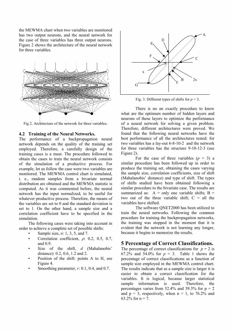
and 0.9. • Size of the shift, d (Mahalanobis’

distance): 0.2, 0.6, 1.2 and 2. • Position of the shift: points A to H, see

Figure 4. • Smoothing parameter, r: 0.1, 0.4, and 0.7.

Fig. 3. Different types of shifts for p = 3.

There is no an exactly procedure to know what are the optimum number of hidden layers and neurons of these layers to optimize the performance of a neural network for solving a given problem. Therefore, different architectures were proved. We found that the following neural networks have the best performance of all the architectures tested: for two variables has a lay-out 6-8-10-2 and the network for three variables has the structure 9-10-12-3 (see Figure 2).

For the case of three variables (p = 3) a similar procedure has been followed up in order to produce the training set, obtaining the cases varying the sample size, correlation coefficients, size of shift (Mahalanobis’ distance) and type of shift. The types of shifts studied have been obtained following a similar procedure to the bivariate case. The results are summarized as: A = only one variable shifts; B = two out of the three variable shift; C = all the variables have shifted.

The software QNET2000 has been utilized to train the neural networks. Following the common procedure for training the backpropagation networks, the training was stopped in the moment that it is evident that the network is not learning any longer, because it begins to memorize the results.

5 Percentage of Correct Classifications. The percentage of correct classifications for p = 2 is 67.2% and 54.0% for p = 3. Table 1 shows the percentage of correct classifications as a function of sample size employed in the MEWMA control chart. The results indicate that as a sample size is larger it is easier to obtain a correct classification for the variables. It is logical, because larger statistical sample information is used. Therefore, the percentages varies from 52.4% and 39.3% for p = 2 and p = 3, respectively, when n = 1, to 76.2% and 63.2% for n = 7.

A D

e

x

2x

F

G H

B

C

E

Simple size n

% correct classifications

p = 2

% correct classifications

p = 3

1 52.4 39.3

3 66.4 53.7

5 73.7 60.1 7 76.2 63.2

Table 1. Correct classifications as function of sample size.

Table 2 shows the percentage of correct classification as a function of the type of shift shown on Figure 4. As it is possible to see, for the same problem that consists of classifying the variables in the groups Shift / No-Shift there is a large variability for the percentage as a function of type of shift. For example, points A and G correspond to the case of the two variables have shifted and the new out-of-control mean vector distances the maximum possible from the previous in-control mean vector (Euclidean distance). In this case, the two values of sample mean to be input in the neural network when the MEWMA chart signals will tend to be very large. So for these cases it will be easy to determine that the two variables have shifted their means. The percentages for the points A and G are not identical (91.4% y 90.7%, respectively) because the employed set to check the efficiency of the neural network is obtained by simulation.

The lowest percentage of correct classifications corresponds to the points D and H (39.7% y 38.8%, respectively). Here we find a case where only one of the means has shifted, and the shift magnitude is small. Therefore, the values of and that will be input to the network will tend to be both small, and in some cases very similar, making very difficult to obtain a correct classification of the variables in the groups Shift / No-Shift. A better percentage is obtained for the points C and F (47.4% and 46.9%, respectively), where also only one variable has shifted, but the shift is of a larger magnitude.

Clearly the neural network detects better the shifts in the cases where both variables have shifted the means. The demonstration of this are the points B and E (78.9% and 79.4%, respectively) where the two means have shifted, buy in a small magnitude. This case seems to have a similar difficulty to the previous cases, but the neural network performs better now.

Table 3 shows the percentage of correct classifications as a function of the type of shift when three variables are monitores. It is reminded that type of point A means that only one variable shifts, B means that two of the three variable shift and C means that all the variables have shifted.

Type of Shift % of Correct

Classifications A 91.4 B 78.9 C 47.4 D 39.7 E 79.4 F 46.9 G 90.7 H 38.8

Table 2. Correct classifications as function of type of shift (p = 2).

Type of Shift % of Correct Classifications

A 65.7 B 55.8 C 38.9

Table 3. Correct classifications as function of type of shift (p = 3).

As it is possible to see, some cases are easier classified than others. Another time the neural network has better efficiency as the number of variables that really have shifted increases. Therefore, if all the variables have shifted the percentage of correct classifications is 65.7%. If two out of three variables have shifted the percentage is 55.8% and the efficiency is 38.9% if only one variable have shifted. The percentages shown on Tables 3 and 4 are similar to the obtained by Aparisi, Avendaño and Sanz (2006) for the Hotelling’s T2 control chart.

Lastly, the percentage of correct classifications as a function of the smoothing parameter in shown on Table 5. The results show that the percentage is larger as the value of the smoothing parameter, r, increases. This behavior is logical, because as r increases the value of the statistic plot,

Q, is more influenced by the sample means, iX ,

used by the neural network to classify the variables. Smoothing parameter

r

% of Correct Classifications

p = 2

% of Correct Classifications

p = 3 0.1 59.2 47.6 0.4 68.9 55.8 0.7 71.1 57.8

Table 4. Correct classification as function of smoothing parameter, r.

6 Software an Example of Application One of the objectives of this work is that the final user can apply the neural network to interpret the signal of the MEWMA chart without being an expert in neural networks. Following this objective software for Windows has been developed. The user only has to input the values of the input nodes and the software shows the classification of the variables in

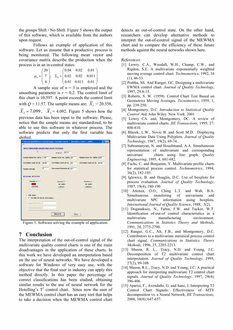
the groups Shift / No-Shift. Figure 5 shows the output of this software, which is available from the authors upon request.

Follows an example of application of this software. Let us assume that a productive process is being monitored. The following mean vector and covariance matrix describe the production when the process is in an in-control states:

0 0

20 0.04 0.02 0.01

7 ; 0.02 0.02 0.011

4 0.01 0.011 0.01

µ = Σ =

A sample size of n = 3 is employed and the smoothing parameter is r = 0.2. The control limit of this chart is 10.597. A point exceeds the control limit

with Q = 11.57. The sample means are: 1X = 20.358,

2 7.099X = , 3X = 4.092. Figure 5 shows how the

previous data has been input to the software. Please, notice that the sample means are standardized, to be able to use this software in whatever process. The software predicts that only the first variable has shifted.

Figure 5. Software solving the example of application.

7 Conclusion The interpretation of the out-of-control signal of the multivariate quality control charts is one of the main disadvantages in the application of these charts. In this work we have developed an interpretation based on the use of neural networks. We have developed a software for Windows of very easy use, with the objective that the final user in industry can apply this method directly. In this paper the percentage of correct classifications has been studied, obtaining similar results to the use of neural network for the Hotelling’s T2 control chart. Since now the user of the MEWMA control chart has an easy tool that helps to take a decision when the MEWMA control chart

detects an out-of-control state. On the other hand, researchers can develop alternative methods to interpret the out-of-control signal of the MEWMA chart and to compare the efficiency of these future methods against the neural networks shown here.

References: [1] Lowry, C.A., Woodall, W.H., Champ, C.W., and

Rigdon, S.E. A multivariate exponentially weighted moving average control chart. Technometrics, 1992, 34 (1), 46-53.

[2] Prabhu, SS. And Runger, GC. Designing a multivariate EWMA control chart. Journal of Quality Technology, 1997, 29:8-15.

[3] Roberts, S. W. (1959). Control Chart Test Based on Geometrics Moving Averages. Tecnometrics, 1959, 1, pp. 239-250.

[4] Montgomery, D.C. Introduction to Statistical Quality Control .4rd. John Wiley. New York. 2001

[5] Lowry CA. and, Montgomery, DC. A review of multivariate control charts. IIE Transactions, 1995; 27: 800-810.

[6] Blazek, L.W., Novic B .and Scott M.D. Displaying Multivariate Data Using Polyplots. Journal of Quality Technology, 1987, 19(2), 69-74.

[7] Subramanyan, N. and Houshmand, A.A. Simultaneous representation of multivariate and corresponding univariate charts using line graph. Quality

Engineering, 1995, 4, 681-682. [8] Fuchs, C. and Benjamin, Y. Multivariate profile charts

for statistical process control. Technometrics, 1994, 36(2), 182-195.

[9] Iglewicz, B. and Hoaglin, D.C. Use of boxplots for process evaluation. Journal of Quality Technology, 1987, 19(4), 180-190.

[10] Atienza, O.O., Ching L.T. and Wah, B.A. Simultaneous monitoring of univariante and multivariate SPC information using boxplots. International Journal of Quality Science, 1988, 3(2).

[11] Doganaksoy, N., Faltin, F.W. and Tucker, W.T. Identification of-out-of control characteristics in a multivariate manufacturing environment. Communications in Statistics Theory and Methods, 1991, 20, 2775-2790.

[12] Runger, G.C., Alt, F.B., and Montgomery, D.C. Contributors to a multivariate statistical process control chart signal. Communications in Statistics. Theory Methods, 1996, 25, 2203-2213.

[13] Mason, R. L., Tracy, N.D. and Young, J.C. Decomposition of T2 multivariate control chart interpretation. Journal of Quality Technology, 1995, 27(2), 99-108.

[14] Mason, R.L., Tracy, N.D. and Young, J.C. A practical approach for interpreting multivariate T2 control chart signals. Journal of Quality Technology, 1997, 29(4), 396-406.

[15] Aparisi, F., Avendaño, G. and Sanz, J. Interpreting T2 Control Chart Signals: Effectiveness of MTY decomposition vs. a Neural Network, IIE Transactions, 2006, 38(8), 647-657.