Interrelationships among Snow Distribution, Snowmelt… · role in determining the timing and magnitude of snow-melt runoff, and the end-of-winter snow distribution is a crucial input

1474 VOLUME 38J O U R N A L O F A P P L I E D M E T E O R O L O G Y

q 1999 American Meteorological Society

Interrelationships among Snow Distribution, Snowmelt, and Snow Cover Depletion:Implications for Atmospheric, Hydrologic, and Ecologic Modeling

GLEN E. LISTON

Department of Atmospheric Science, Colorado State University, Fort Collins, Colorado

(Manuscript received 5 October 1998, in final form 21 December 1998)

ABSTRACT

Local, regional, and global atmospheric, hydrologic, and ecologic models used to simulate weather, climate,land surface moisture, and vegetation processes all commonly represent their computational domains by acollection of finite areas or grid cells. Within each of these cells three fundamental features are required todescribe the evolution of seasonal snow cover from the end of winter through spring melt. These three featuresare 1) the within-grid snow water equivalent (SWE) distribution, 2) the gridcell melt rate, and 3) the within-grid depletion of snow-covered area. This paper defines the exact mathematical interrelationships among thesethree features and demonstrates how knowledge of any two of them allows generation of the third. Duringsnowmelt, the spatially variable subgrid SWE depth distribution is largely responsible for the patchy mosaic ofsnow and vegetation that develops as the snow melts. Applying the melt rate to the within-grid snow distributionleads to the exposure of vegetation, and the subgrid-scale vegetation exposure influences the snowmelt rate andthe grid-averaged surface fluxes. By using the developed interrelationships, the fundamental subgrid-scale featuresof the seasonal snow cover evolution and the associated energy and moisture fluxes can be simulated using acombination of remote sensing products that define the snow-covered area evolution and a submodel thatappropriately handles the snowmelt computation. Alternatively, knowledge of the subgrid SWE distribution canbe used as a substitute for the snow-covered area information.

1. Introduction

With its high albedo, low thermal conductivity, andconsiderable spatial and temporal variability, seasonalsnow cover overlying land plays a key role in governingthe earth’s global radiation balance; this balance is theprimary driver of the earth’s atmospheric circulationsystem and associated climate. Of the various featuresthat influence the surface radiation balance, the locationand duration of snow cover compose two of the mostimportant seasonal variables. In the Northern Hemi-sphere the mean monthly land area covered by snowranges from 7% to 40% during the annual cycle, makingsnow cover the most rapidly varying large-scale surfacefeature on the earth (Hall 1988).

The problem of realistically representing seasonalsnow in regional and global atmospheric and hydrologicmodels is made complex because of the numerous snow-related features that display considerable spatial vari-ability at scales below those resolved by the models. Asan example of this variability, over the winter landscapein middle and high latitudes the interactions among wind,

Corresponding author address: Dr. Glen E. Liston, Dept. of At-mospheric Science, Colorado State University, Fort Collins, CO 80523.E-mail: [email protected]

vegetation, topography, precipitation, solar radiation, andsnowfall produce snow covers of nonuniform depth anddensity (e.g., Liston and Sturm 1998). During the meltof these snow covers, the snow-depth variation leads toa patchy mosaic of vegetation and snow cover thatevolves as the snow melts (e.g., Shook et al. 1993). Thismix of snow and vegetation strongly influences the en-ergy fluxes returned to the atmosphere and the associatedfeedbacks that accelerate the melting of remaining snow-covered areas. From the perspective of a surface energybalance, the interactions between the land and atmo-sphere are particularly complex during this melt period(Liston 1995; Essery 1997; Neumann and Marsh 1998).The variable snow distribution also can play an importantrole in determining the timing and magnitude of snow-melt runoff, and the end-of-winter snow distribution is acrucial input to snowmelt hydrology models, includingthose used for water resource management (e.g., U.S.Army Corps of Engineers 1956; Male and Gray 1981;Martinec and Rango 1986; WMO 1986; Kane et al.1991). In Arctic tundra and alpine regions the unevendistribution of snow exerts strong control over plant com-munity distribution (Evans et al. 1989; Walker et al.1993), and in the forest–alpine ecotone the snow distri-bution influences tree distributions and growth charac-teristics (Griggs 1938; Billings 1969; Daly 1984; Woold-ridge et al. 1996).

OCTOBER 1999 1475L I S T O N

In light of the role that snow plays in influencing landand atmospheric processes, it is essential that local, re-gional, and global models used to simulate weather, cli-mate, hydrologic, and ecologic interactions be capableof accurately describing the seasonal snow evolution.In recent years, significant strides have been made torepresent snow cover better in climate models (Verseghy1991; Lynch-Stieglitz 1994; Marshall and Oglesby1994; Marshall et al. 1994; Douville et al. 1995; Yanget al. 1997; Loth and Graf 1998a; Slater et al. 1998),but there are still studies that indicate that current cli-mate model simulations of seasonal snow do not repro-duce the observed snow distributions (e.g., Foster et al.1996). Typically, snow accumulation and melt in cli-mate models are simulated by applying simple energyand mass balance accounting procedures (Foster et al.1996). These algorithms frequently neglect or oversim-plify important physical processes such as those asso-ciated with subgrid-scale temporal and spatial variabil-ity of snow-covered area. The lack of subgrid snowdistribution representations in most climate models hasbeen acknowledged as a deficiency in snow cover evo-lution and atmospheric interaction simulations (Lothand Graf 1998b). Walland and Simmonds (1996) intro-duced one method to address this deficiency. To accountfor snow distribution–related processes in weather, cli-mate, hydrologic, and ecologic models, accurate de-scriptions of grid-scale and subgrid-scale snow distri-butions are necessary.

At its most basic foundation, capturing the funda-mental aspects of snow cover evolution within a modelgrid cell requires addressing three primary features.Conceptually, these three relate directly to

1) the snow cover has some spatial distribution (forexample, over a parking lot or a relatively flat prairielandscape the distribution generally is uniform, whilein windblown and topographically variable regionsthe distribution can be quite nonuniform),

2) at some point during the year the snow cover ex-periences melting, and

3) eventually, as part of the snowmelt process, the snowcover disappears and exposes the underlying surface(usually soil and low-growing vegetation).

While at first glance these three features may appearoverly simplistic, they are coupled so strongly that anyunrealistic model gridcell description of one of themleads to the misrepresentation of the others. This mis-representation, in turn, has important consequences formodel-computed energy and moisture fluxes.

Through a combination of meteorological observa-tions, spatially distributed snow water equivalent (SWE)depth measurements, and snow cover depletion obser-vations, Liston (1986) suggested that there must be astrong interrelationship among snowmelt, snow distri-bution, and snow cover depletion. Cline et al. (1998)discussed and applied a ‘‘conceptual’’ snow cover de-pletion model in which the premelt SWE depth is a func-

tion of snow cover duration and accumulated melt energyat a particular site, and similar relationships have beenused implicitly as part of other, primarily hydrologic,studies (e.g., Dunne and Leopold 1978; Rango and Mar-tinec 1979; Martinec and Rango 1981, 1987; Ferguson1984; Buttle and McDonnell 1987; Rango 1993; Cline1997; Konig and Sturm 1998). While these studies have,in some way, made use of the relationships among snowcover melt, distribution, and areal depletion, the exactmathematical interrelationships that form the basis ofthese studies have never been defined, and a more explicitand complete discussion of these features is warranted.This paper provides a mathematical description of thegeneral conceptual model that has been used in the pastand lays the foundation for the next generation of modelsthat will include improved realism in their snow distri-bution representations. This mathematical descriptionwill formalize the general assumptions adopted in thehydrologic studies cited above and will provide a soundtheoretical framework for implementing these ideas inatmospheric and ecologic models. In addition, it will pro-vide valuable insight into how these interrelationshipscan be used to improve seasonal snow cover simulations.Specifically, the mathematical interrelationships amongsnow cover melt, snow distribution, and snow cover arealdepletion within a model grid cell will be presented anddiscussed within the context of atmospheric, hydrologic,and ecologic modeling efforts.

2. Mathematical formulation

Initially, for the purpose of the following presenta-tion, the natural system that will be discussed will followthe snow evolution pattern observed in much of theArctic, where the seasons are well defined; winter islargely a period of snow accumulation and no melting,and spring is largely a period of melting and no snowaccumulation. Thus, winter leads to an end-of-wintersnow distribution and is followed by a spring melt pe-riod that proceeds until the snow is gone. In middlelatitudes, the snow cover generally undergoes numeroussuch ‘‘winter–spring’’ events during the course of ayear; the relaxation of this simplified ‘‘arctic’’ behaviorwill be discussed later in this paper. In addition, it isunderstood that from the perspective of the atmosphereand large-feature hydrologic system the first-order effectis whether there is snow on the ground; this importancearises primarily because of the large albedo differencesbetween snow and other (nonice) surfaces and the max-imum 08C snow surface temperature constraint (e.g.,Liston 1995). These two factors dominate the gridcellsurface energy balance to the extent that it is not pos-sible, without significantly misrepresenting the govern-ing physics, to simulate the correct moisture and energyfluxes unless the gridcell snow-covered fraction isknown. To simplify the discussion it also is assumedthat the bulk, or vertically integrated, average snow den-sity is known; thus, the terms ‘‘snow depth’’ and ‘‘SWE


depth’’ will be used interchangeably, with the under-standing that the snow depths always can be convertedto an SWE depth by applying the snow (and water)density. The term ‘‘melt rate’’ refers to moisture lostfrom the snow cover, and the ‘‘exposure of vegetation’’refers to exposing the surface that was previously cov-ered by snow. This surface can be any type, includingthe low-stature rock, low-growing vegetation, and bareground found on the prairies and in Arctic and alpineregions, or it can be the surfaces found under deciduousand evergreen forest canopies.

Under the simple Arctic-type winter–spring snow his-tory, for each model grid cell three fundamental featuresare required to describe the evolution of snow coverfrom the end of winter through spring melt. These threefundamental features are

1) the end-of-winter (premelt) SWE distribution,2) the melt rate, and3) the depletion of snow-covered area.

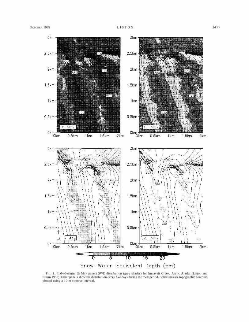
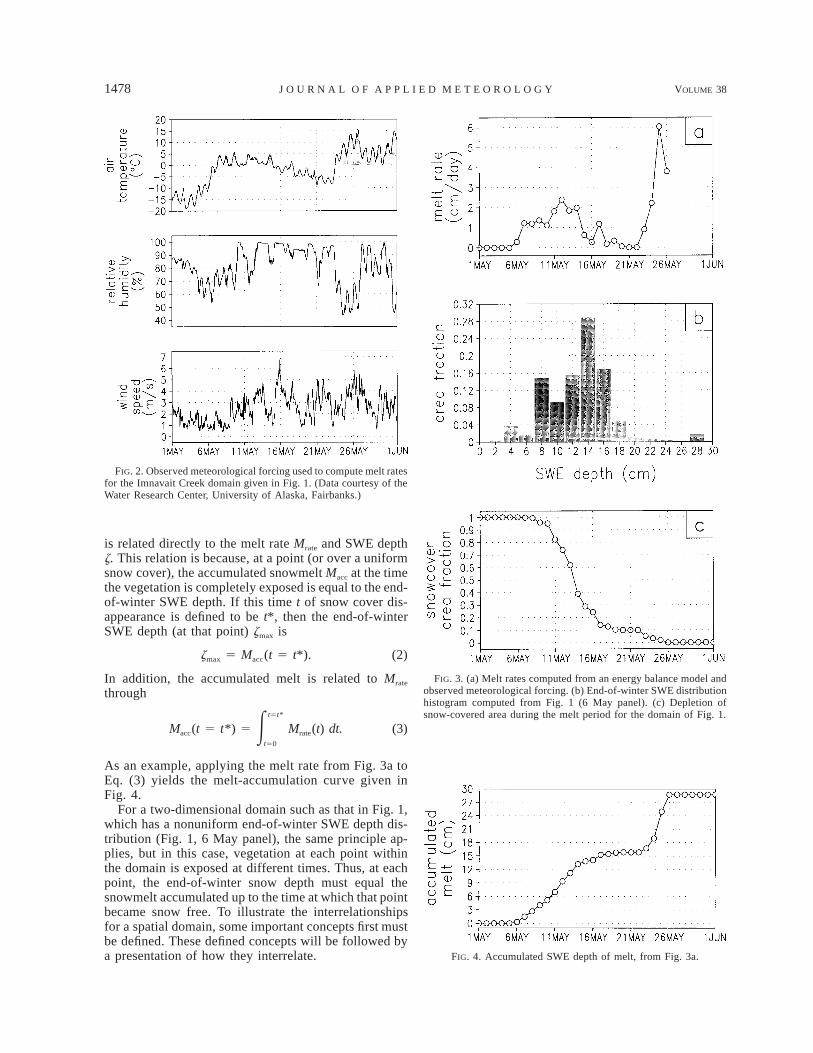
Throughout this paper, an Arctic Alaska example inwhich snow distribution and atmospheric-forcing dataare known will be used to help to illustrate the inter-relationships among these three features. This examplecan be considered to represent an atmospheric, hydro-logic, or ecologic model grid cell. Figure 1 (6 Maypanel) describes the example snow distribution takenfrom Imnavait Creek, Alaska (Liston and Sturm 1998).This area is located between the headwaters of the Ku-paruk and Toolik Rivers at 688379N, 1498179W and anelevation of approximately 900 m. The vegetation cov-ering the site is composed of low-growing sedges andgrasses roughly 15 cm in height and occasional group-ings of taller willows approximately 40 cm high, locatedin hillside water tracts and valley bottoms. Tussock tun-dra covers much of the area, with swampy features inthe valley bottoms and dry rocky outcroppings on theexposed ridges. The topography is characterized bygently rolling ridges and valleys that have wavelengthsof 1–2 km and amplitudes of 25–75 m (Fig. 1). Alsowithin the domain are several more-pronounced topo-graphic features that have much shorter and steeperslopes (up to 308 slopes over distances of a few tens ofmeters). The prevailing winds in Fig. 1 are from thesouthwest and lead to erosion on south- and west-facingslopes and increased snow accumulations on north- andeast-facing slopes. Figure 2 summarizes the examplehourly meteorological forcing, assumed to be represen-tative over the domain of Fig. 1. These meteorologicalobservations were collected from a tower located at ap-proximately 2 km north and 1.2 km east in the Fig. 1domain and were provided by the Water Research Cen-ter, University of Alaska, Fairbanks.

The three fundamental features required to describethe snow cover evolution can be generated from Figs.1 and 2. The atmospheric forcing data of Fig. 2 are usedto compute the snowmelt rate (Fig. 3a) by applying thesurface energy balance model

(1 2 a)Qsi 1 Qli 1 Qle 1 Qh 1 Qe 1 Qc 5 Qm, (1)

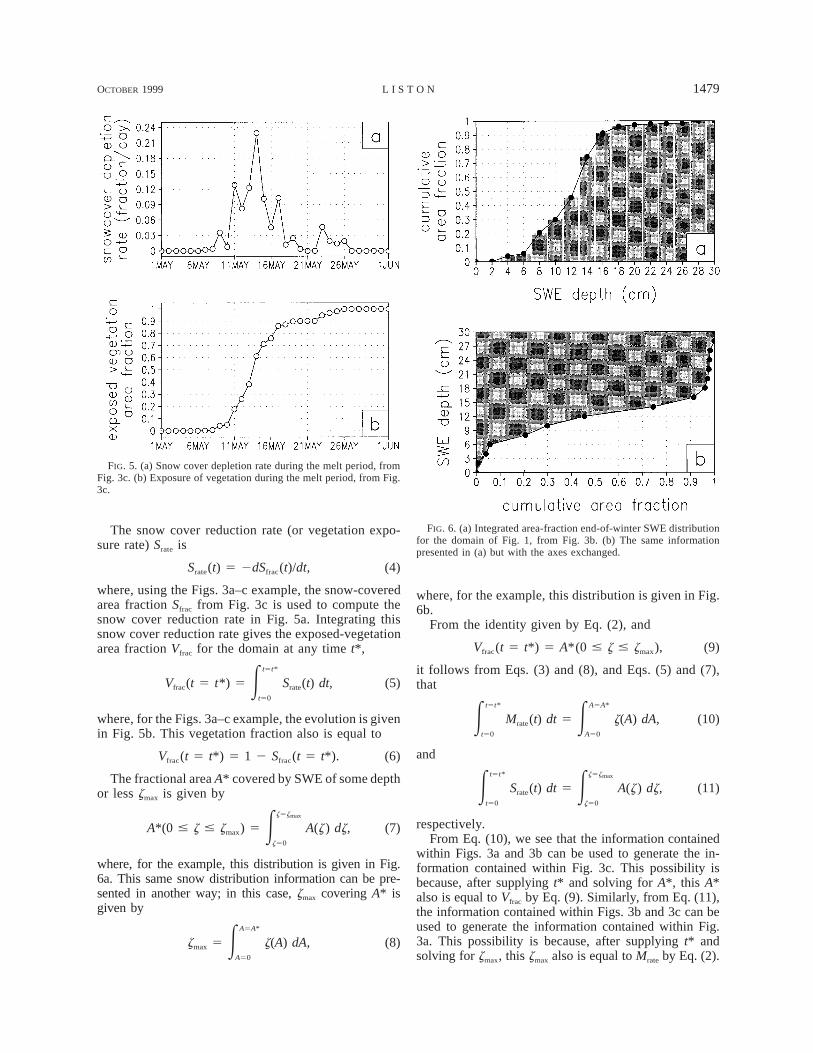
where Qsi is the solar radiation reaching the surface ofthe earth, Qli is the incoming longwave radiation, Qle isthe emitted longwave radiation, Qh is the turbulent ex-change of sensible heat, Qe is the turbulent exchange oflatent heat, Qc is the conductive energy transport, Qm isthe energy flux available for melt, and a is the surfacealbedo. Details of the formulation of each term in Eq.(1) and the model solution can be found in Liston (1995),Liston and Hall (1995), and Liston et al. (1999b). In thismodel, each term in the surface energy balance is com-puted by applying general equations that have been castin a form that leaves the surface temperature as the onlyunknown. The melt energy is defined to be zero, and Eq.(1) is solved iteratively for the surface temperature. Inthe presence of snow, resultant surface temperaturesgreater than 08C indicate that energy is available for melt-ing. The amount of available melt energy then is com-puted by fixing the surface temperature at 08C and solvingEq. (1) for Qm. Under melting conditions, the snow sur-face is considered to be fully saturated and verticallyisothermal. For the purposes of the current discussion,this melt rate equals the moisture lost from the snowcover (although it is recognized that in the natural systemthere may be delays between melt and snow cover mois-ture loss caused by such processes as percolation andrefreezing). The end-of-winter snow distribution of Fig.1 (6 May panel) is presented as a histogram in Fig. 3b,and applying the daily melt rates from Fig. 3a to thedistribution of Fig. 1 yields the snow cover depletion inFig. 3c. Implicit in this approach is that the melt ratesof Fig. 3a are applicable to the entire domain given inFig. 1 and represented by Figs. 3b and 3c.

Figures 3a–c are interrelated strongly and knowledgeof any two of them allows the generation of the third.When the melt rates of Fig. 3a are applied to the snowdistribution of Fig. 3b, the snow-covered area is de-pleted according to the curve in Fig. 3c. It is not soobvious that the melt rates (Fig. 3a) can be derived fromthe snow cover depletion (Fig. 3c) and the snow dis-tribution (Fig. 3b). Last, and maybe even more impor-tant, is that the snow distribution (Fig. 3b) can be de-rived from the melt rates (Fig. 3a) and the snow coverdepletion (Fig. 3c). This last point has major implica-tions for regional- and global-scale atmospheric and hy-drologic modeling because melt rates can be computedfrom readily available atmospheric quantities (such asthose collected as part of local and worldwide obser-vational networks and those generated at atmosphericanalysis and forecast centers), and the snow cover de-pletion curves are becoming readily available as part ofNational Aeronautics and Space Administration(NASA) (Hall et al. 1995) and National OperationalHydrologic Remote Sensing Center (NOHRSC) (http://www.nohrsc.nws.gov/) (Carroll 1997) snow cover re-mote sensing programs.

The exposure of vegetation (or loss of snow cover)


FIG. 1. End-of-winter (6 May panel) SWE distribution (gray shades) for Imnavait Creek, Arctic Alaska (Liston andSturm 1998). Other panels show the distribution every five days during the melt period. Solid lines are topographic contoursplotted using a 10-m contour interval.


FIG. 2. Observed meteorological forcing used to compute melt ratesfor the Imnavait Creek domain given in Fig. 1. (Data courtesy of theWater Research Center, University of Alaska, Fairbanks.)

FIG. 3. (a) Melt rates computed from an energy balance model andobserved meteorological forcing. (b) End-of-winter SWE distributionhistogram computed from Fig. 1 (6 May panel). (c) Depletion ofsnow-covered area during the melt period for the domain of Fig. 1.

FIG. 4. Accumulated SWE depth of melt, from Fig. 3a.

is related directly to the melt rate Mrate and SWE depthz. This relation is because, at a point (or over a uniformsnow cover), the accumulated snowmelt Macc at the timethe vegetation is completely exposed is equal to the end-of-winter SWE depth. If this time t of snow cover dis-appearance is defined to be t*, then the end-of-winterSWE depth (at that point) zmax is

zmax 5 Macc(t 5 t*). (2)

In addition, the accumulated melt is related to Mrate

through

t5t*

M (t 5 t*) 5 M (t) dt. (3)acc E rate

t50

As an example, applying the melt rate from Fig. 3a toEq. (3) yields the melt-accumulation curve given inFig. 4.

For a two-dimensional domain such as that in Fig. 1,which has a nonuniform end-of-winter SWE depth dis-tribution (Fig. 1, 6 May panel), the same principle ap-plies, but in this case, vegetation at each point withinthe domain is exposed at different times. Thus, at eachpoint, the end-of-winter snow depth must equal thesnowmelt accumulated up to the time at which that pointbecame snow free. To illustrate the interrelationshipsfor a spatial domain, some important concepts first mustbe defined. These defined concepts will be followed bya presentation of how they interrelate.


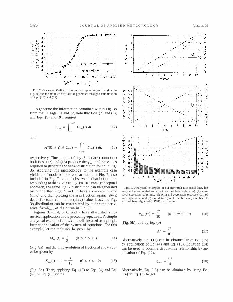
FIG. 5. (a) Snow cover depletion rate during the melt period, fromFig. 3c. (b) Exposure of vegetation during the melt period, from Fig.3c.

FIG. 6. (a) Integrated area-fraction end-of-winter SWE distributionfor the domain of Fig. 1, from Fig. 3b. (b) The same informationpresented in (a) but with the axes exchanged.

The snow cover reduction rate (or vegetation expo-sure rate) Srate is

Srate(t) 5 2dSfrac(t)/dt, (4)

where, using the Figs. 3a–c example, the snow-coveredarea fraction Sfrac from Fig. 3c is used to compute thesnow cover reduction rate in Fig. 5a. Integrating thissnow cover reduction rate gives the exposed-vegetationarea fraction Vfrac for the domain at any time t*,

t5t*

V (t 5 t*) 5 S (t) dt, (5)frac E rate

t50

where, for the Figs. 3a–c example, the evolution is givenin Fig. 5b. This vegetation fraction also is equal to

Vfrac(t 5 t*) 5 1 2 Sfrac(t 5 t*). (6)

The fractional area A* covered by SWE of some depthor less zmax is given by

z5zmax

A*(0 # z # z ) 5 A(z) dz, (7)max Ez50

where, for the example, this distribution is given in Fig.6a. This same snow distribution information can be pre-sented in another way; in this case, zmax covering A* isgiven by

A5A*

z 5 z(A) dA, (8)max EA50

where, for the example, this distribution is given in Fig.6b.

From the identity given by Eq. (2), and

Vfrac(t 5 t*) 5 A*(0 # z # zmax), (9)

it follows from Eqs. (3) and (8), and Eqs. (5) and (7),that

t5t* A5A*

M (t) dt 5 z(A) dA, (10)E rate Et50 A50

andt5t* z5zmax

S (t) dt 5 A(z) dz, (11)E rate Et50 z50

respectively.From Eq. (10), we see that the information contained

within Figs. 3a and 3b can be used to generate the in-formation contained within Fig. 3c. This possibility isbecause, after supplying t* and solving for A*, this A*also is equal to Vfrac by Eq. (9). Similarly, from Eq. (11),the information contained within Figs. 3b and 3c can beused to generate the information contained within Fig.3a. This possibility is because, after supplying t* andsolving for zmax, this zmax also is equal to Mrate by Eq. (2).


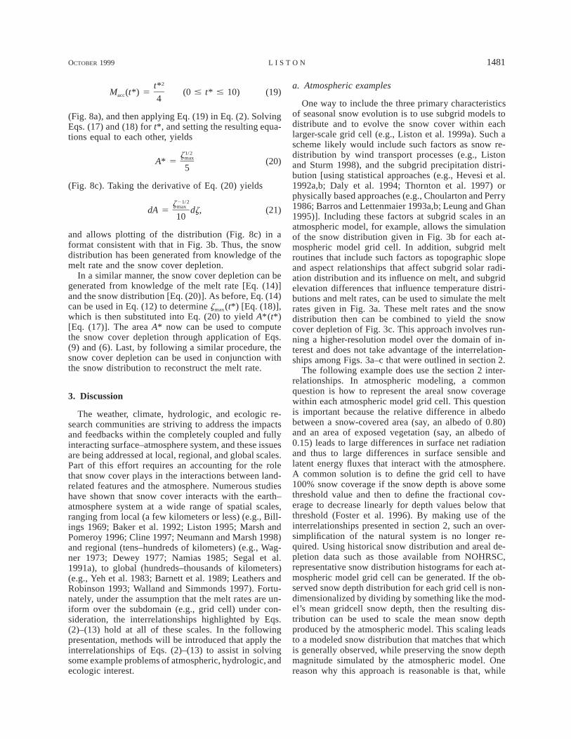
FIG. 7. Observed SWE distribution corresponding to that given inFig. 6a, and the modeled distribution generated through a combinationof Eqs. (12) and (13).

FIG. 8. Analytical examples of (a) snowmelt rate (solid line, leftaxis) and accumulated snowmelt (dashed line, right axis), (b) snowcover depletion (solid line, left axis) and vegetation exposure (dashedline, right axis), and (c) cumulative (solid line, left axis) and discrete(shaded bars, right axis) SWE distribution.

To generate the information contained within Fig. 3bfrom that in Figs. 3a and 3c, note that Eqs. (2) and (3),and Eqs. (5) and (9), suggest

t5t*

z 5 M (t) dt (12)max E rate

t50

and

t5t*

A*(0 # z # z ) 5 S (t) dt, (13)max E rate

t50

respectively. Thus, inputs of any t* that are common toboth Eqs. (12) and (13) produce the zmax and A* valuesrequired to generate the snow distribution found in Fig.3b. Applying this methodology to the example caseyields the ‘‘modeled’’ snow distribution in Fig. 7; alsoincluded in Fig. 7 is the ‘‘observed’’ distribution cor-responding to that given in Fig. 6a. In a more conceptualapproach, the same Fig. 7 distribution can be generatedby noting that Figs. 4 and 5b have a common x axis(time) and then plotting the area fraction against SWEdepth for each common x (time) value. Last, the Fig.3b distribution can be constructed by taking the deriv-ative dA*/dzmax of the curve in Fig. 7.

Figures 3a–c, 4, 5, 6, and 7 have illustrated a nu-merical application of the preceding equations. A simpleanalytical example follows and will be used to highlightfurther application of the system of equations. For thisexample, let the melt rate be given by

tM (t) 5 (0 # t # 10) (14)rate 2

(Fig. 8a), and the time evolution of fractional snow cov-er be given by

tS (t) 5 1 2 (0 # t # 10) (15)frac 10

(Fig. 8b). Then, applying Eq. (15) to Eqs. (4) and Eq.(5), or Eq. (6), yields

t*V (t*) 5 (0 # t* # 10) (16)frac 10

(Fig. 8b), and by Eq. (9)

t*A* 5 . (17)

10

Alternatively, Eq. (17) can be obtained from Eq. (15)by application of Eq. (4) and Eq. (13). Equation (14)can be used to obtain a depth–time relationship by ap-plication of Eq. (12),

2t*z 5 . (18)max 4

Alternatively, Eq. (18) can be obtained by using Eq.(14) in Eq. (3) to get


2t*M (t*) 5 (0 # t* # 10) (19)acc 4

(Fig. 8a), and then applying Eq. (19) in Eq. (2). SolvingEqs. (17) and (18) for t*, and setting the resulting equa-tions equal to each other, yields

1/2zmaxA* 5 (20)5

(Fig. 8c). Taking the derivative of Eq. (20) yields

21/2zmaxdA 5 dz, (21)10

and allows plotting of the distribution (Fig. 8c) in aformat consistent with that in Fig. 3b. Thus, the snowdistribution has been generated from knowledge of themelt rate and the snow cover depletion.

In a similar manner, the snow cover depletion can begenerated from knowledge of the melt rate [Eq. (14)]and the snow distribution [Eq. (20)]. As before, Eq. (14)can be used in Eq. (12) to determine zmax(t*) [Eq. (18)],which is then substituted into Eq. (20) to yield A*(t*)[Eq. (17)]. The area A* now can be used to computethe snow cover depletion through application of Eqs.(9) and (6). Last, by following a similar procedure, thesnow cover depletion can be used in conjunction withthe snow distribution to reconstruct the melt rate.

3. Discussion

The weather, climate, hydrologic, and ecologic re-search communities are striving to address the impactsand feedbacks within the completely coupled and fullyinteracting surface–atmosphere system, and these issuesare being addressed at local, regional, and global scales.Part of this effort requires an accounting for the rolethat snow cover plays in the interactions between land-related features and the atmosphere. Numerous studieshave shown that snow cover interacts with the earth–atmosphere system at a wide range of spatial scales,ranging from local (a few kilometers or less) (e.g., Bill-ings 1969; Baker et al. 1992; Liston 1995; Marsh andPomeroy 1996; Cline 1997; Neumann and Marsh 1998)and regional (tens–hundreds of kilometers) (e.g., Wag-ner 1973; Dewey 1977; Namias 1985; Segal et al.1991a), to global (hundreds–thousands of kilometers)(e.g., Yeh et al. 1983; Barnett et al. 1989; Leathers andRobinson 1993; Walland and Simmonds 1997). Fortu-nately, under the assumption that the melt rates are un-iform over the subdomain (e.g., grid cell) under con-sideration, the interrelationships highlighted by Eqs.(2)–(13) hold at all of these scales. In the followingpresentation, methods will be introduced that apply theinterrelationships of Eqs. (2)–(13) to assist in solvingsome example problems of atmospheric, hydrologic, andecologic interest.

a. Atmospheric examples

One way to include the three primary characteristicsof seasonal snow evolution is to use subgrid models todistribute and to evolve the snow cover within eachlarger-scale grid cell (e.g., Liston et al. 1999a). Such ascheme likely would include such factors as snow re-distribution by wind transport processes (e.g., Listonand Sturm 1998), and the subgrid precipitation distri-bution [using statistical approaches (e.g., Hevesi et al.1992a,b; Daly et al. 1994; Thornton et al. 1997) orphysically based approaches (e.g., Choularton and Perry1986; Barros and Lettenmaier 1993a,b; Leung and Ghan1995)]. Including these factors at subgrid scales in anatmospheric model, for example, allows the simulationof the snow distribution given in Fig. 3b for each at-mospheric model grid cell. In addition, subgrid meltroutines that include such factors as topographic slopeand aspect relationships that affect subgrid solar radi-ation distribution and its influence on melt, and subgridelevation differences that influence temperature distri-butions and melt rates, can be used to simulate the meltrates given in Fig. 3a. These melt rates and the snowdistribution then can be combined to yield the snowcover depletion of Fig. 3c. This approach involves run-ning a higher-resolution model over the domain of in-terest and does not take advantage of the interrelation-ships among Figs. 3a–c that were outlined in section 2.

The following example does use the section 2 inter-relationships. In atmospheric modeling, a commonquestion is how to represent the areal snow coveragewithin each atmospheric model grid cell. This questionis important because the relative difference in albedobetween a snow-covered area (say, an albedo of 0.80)and an area of exposed vegetation (say, an albedo of0.15) leads to large differences in surface net radiationand thus to large differences in surface sensible andlatent energy fluxes that interact with the atmosphere.A common solution is to define the grid cell to have100% snow coverage if the snow depth is above somethreshold value and then to define the fractional cov-erage to decrease linearly for depth values below thatthreshold (Foster et al. 1996). By making use of theinterrelationships presented in section 2, such an over-simplification of the natural system is no longer re-quired. Using historical snow distribution and areal de-pletion data such as those available from NOHRSC,representative snow distribution histograms for each at-mospheric model grid cell can be generated. If the ob-served snow depth distribution for each grid cell is non-dimensionalized by dividing by something like the mod-el’s mean gridcell snow depth, then the resulting dis-tribution can be used to scale the mean snow depthproduced by the atmospheric model. This scaling leadsto a modeled snow distribution that matches that whichis generally observed, while preserving the snow depthmagnitude simulated by the atmospheric model. Onereason why this approach is reasonable is that, while


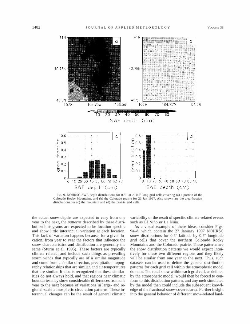
FIG. 9. NOHRSC SWE depth distributions for 0.58 lat 3 0.58 long grid cells covering (a) a portion of theColorado Rocky Mountains, and (b) the Colorado prairie for 23 Jan 1997. Also shown are the area-fractiondistributions for (c) the mountain and (d) the prairie grid cells.

the actual snow depths are expected to vary from oneyear to the next, the patterns described by these distri-bution histograms are expected to be location specificand show little interannual variation at each location.This lack of variation happens because, for a given lo-cation, from year to year the factors that influence thesnow characteristics and distribution are generally thesame (Sturm et al. 1995). These factors are typicallyclimate related, and include such things as prevailingstorm winds that typically are of a similar magnitudeand come from a similar direction, precipitation–topog-raphy relationships that are similar, and air temperaturesthat are similar. It also is recognized that these similar-ities do not always hold, and that regions near climaticboundaries may show considerable differences from oneyear to the next because of variations in large- and re-gional-scale atmospheric circulation patterns. These in-terannual changes can be the result of general climatic

variability or the result of specific climate-related eventssuch as El Nino or La Nina.

As a visual example of these ideas, consider Figs.9a–d, which contain the 23 January 1997 NOHRSCsnow distributions for 0.58 latitude by 0.58 longitudegrid cells that cover the northern Colorado RockyMountains and the Colorado prairie. These patterns arethe snow distribution patterns we would expect intui-tively for these two different regions and they likelywill be similar from one year to the next. Thus, suchdatasets can be used to define the general distributionpatterns for each grid cell within the atmospheric modeldomain. The total snow within each grid cell, as definedby the atmospheric model, would then be forced to con-form to this distribution pattern, and any melt simulatedby the model then could include the subsequent knowl-edge of the fractional snow-covered area. Further insightinto the general behavior of different snow-related land-


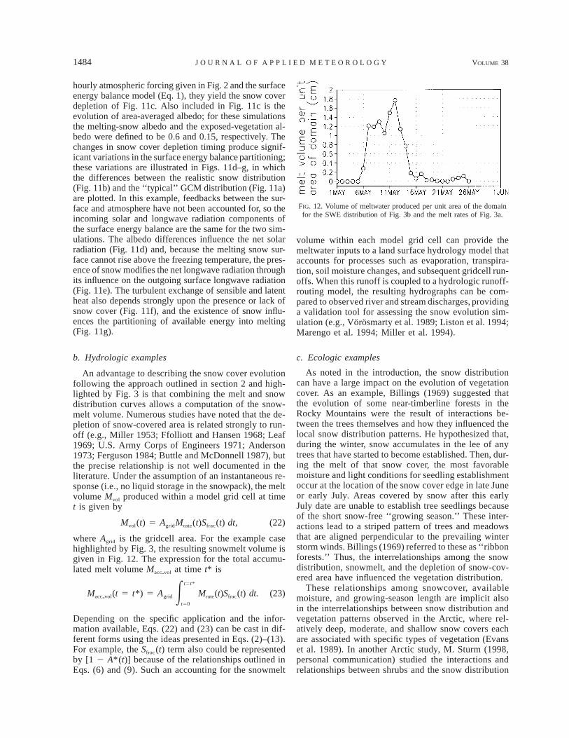
FIG. 10. Evolution of snow-covered area for the mountainous do-main of Fig. 9a and for the prairie domain of Fig. 9b. These curveswere generated using NOHRSC snow distribution observations,where the markers indicate observation dates.

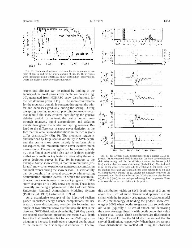
FIG. 11. (a) Gridcell SWE distributions using a typical GCM ap-proach. (b) An observed SWE distribution. (c) Snow cover depletion(left axis) during melt for the GCM-type snow distribution (solidline) and the observed snow distribution (dashed line). Also includedin (c) is the gridcell-averaged albedo evolution (right axis), wherethe melting-snow and vegetation albedos were defined to be 0.6 and0.15, respectively. Panels (d)–(g) display the difference between theobserved snow distribution (b) and the GCM-type snow distribution(a), that is, (b)–(a), for the melt-period energy flux components. Flux-es toward the surface are defined to be positive.

scapes and climates can be gained by looking at theJanuary–June areal snow cover depletion curves (Fig.10), generated from NOHRSC snow distributions, forthe two domains given in Fig. 9. The snow-covered areafor the mountain domain is constant throughout the win-ter and decreases gradually during the spring. Duringthe spring months, mountain precipitation events occurthat rebuild the snow-covered area during the generalablation period. In contrast, the prairie domain goesthrough relatively rapid accumulation and ablationevents throughout the winter and spring seasons. Re-lated to the differences in snow cover depletion is thefact that the areal snow distributions in the two regionsdiffer dramatically (Fig. 9). The mountain region ischaracterized by large spatial variability in SWE depth,and the prairie snow cover largely is uniform. As aconsequence, the mountain snow cover evolves muchmore slowly. The prairie region can be covered quicklyby a thin film of snow and it also can be depleted quicklyas that snow melts. A key feature illustrated by the snowcover depletion curves in Fig. 10, in contrast to theexample Arctic snow cover, is that the midlatitude (Co-lorado) snow cover experiences numerous accumulationand melt events during the snow season. This variabilitycan be thought of as several arctic-type winter–springaccumulation–ablation events, in which the accumula-tion and melt events may or may not progress to 100%snow coverage or to 100% snow depletion. These ideascurrently are being implemented in the Colorado StateUniversity Regional Atmospheric Modeling System(Pielke et al. 1992; Liston et al. 1999a).

As a quantitative example of the improved realismgained in surface energy balance computations that userealistic snow distributions, consider the following ex-ample of two different snow distributions: the first is theobserved SWE distribution given in Fig. 1 (6 May panel);the second distribution preserves the mean SWE depthfrom the first distribution but forces the SWE depth dis-tribution to increase linearly over a range of depths equalto the mean of the first sample distribution 6 1.5 cm;

this distribution yields an SWE depth range of 3 cm, orabout 10–15 cm of snow. This second approach is con-sistent with the frequently used general circulation model(GCM) methodology of holding the gridcell snow cov-erage at 100% when depths are greater than some thresh-old value (typically 5–15 cm of snow), and decreasingthe snow coverage linearly with depth below that value(Foster et al. 1996). These distributions are illustrated inFigs. 11a and 11b for the GCM distribution and the ob-served distribution, respectively. When these two samplesnow distributions are melted off using the observed


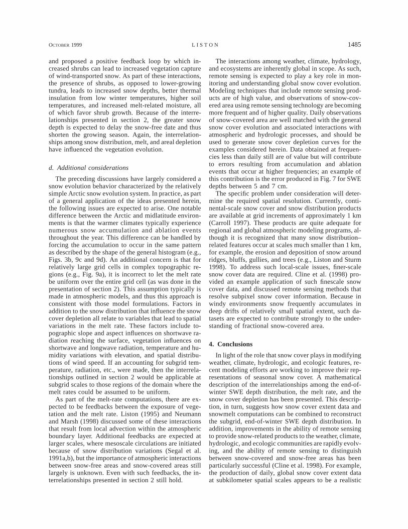
FIG. 12. Volume of meltwater produced per unit area of the domainfor the SWE distribution of Fig. 3b and the melt rates of Fig. 3a.

hourly atmospheric forcing given in Fig. 2 and the surfaceenergy balance model (Eq. 1), they yield the snow coverdepletion of Fig. 11c. Also included in Fig. 11c is theevolution of area-averaged albedo; for these simulationsthe melting-snow albedo and the exposed-vegetation al-bedo were defined to be 0.6 and 0.15, respectively. Thechanges in snow cover depletion timing produce signif-icant variations in the surface energy balance partitioning;these variations are illustrated in Figs. 11d–g, in whichthe differences between the realistic snow distribution(Fig. 11b) and the ‘‘typical’’ GCM distribution (Fig. 11a)are plotted. In this example, feedbacks between the sur-face and atmosphere have not been accounted for, so theincoming solar and longwave radiation components ofthe surface energy balance are the same for the two sim-ulations. The albedo differences influence the net solarradiation (Fig. 11d) and, because the melting snow sur-face cannot rise above the freezing temperature, the pres-ence of snow modifies the net longwave radiation throughits influence on the outgoing surface longwave radiation(Fig. 11e). The turbulent exchange of sensible and latentheat also depends strongly upon the presence or lack ofsnow cover (Fig. 11f), and the existence of snow influ-ences the partitioning of available energy into melting(Fig. 11g).

b. Hydrologic examples

An advantage to describing the snow cover evolutionfollowing the approach outlined in section 2 and high-lighted by Fig. 3 is that combining the melt and snowdistribution curves allows a computation of the snow-melt volume. Numerous studies have noted that the de-pletion of snow-covered area is related strongly to run-off (e.g., Miller 1953; Ffolliott and Hansen 1968; Leaf1969; U.S. Army Corps of Engineers 1971; Anderson1973; Ferguson 1984; Buttle and McDonnell 1987), butthe precise relationship is not well documented in theliterature. Under the assumption of an instantaneous re-sponse (i.e., no liquid storage in the snowpack), the meltvolume Mvol produced within a model grid cell at timet is given by

Mvol(t) 5 AgridMrate(t)Sfrac(t) dt, (22)

where Agrid is the gridcell area. For the example casehighlighted by Fig. 3, the resulting snowmelt volume isgiven in Fig. 12. The expression for the total accumu-lated melt volume Maccpvol at time t* is

t5t*

M (t 5 t*) 5 A M (t)S (t) dt. (23)accpvol grid E rate frac

t50

Depending on the specific application and the infor-mation available, Eqs. (22) and (23) can be cast in dif-ferent forms using the ideas presented in Eqs. (2)–(13).For example, the Sfrac(t) term also could be representedby [1 2 A*(t)] because of the relationships outlined inEqs. (6) and (9). Such an accounting for the snowmelt

volume within each model grid cell can provide themeltwater inputs to a land surface hydrology model thataccounts for processes such as evaporation, transpira-tion, soil moisture changes, and subsequent gridcell run-offs. When this runoff is coupled to a hydrologic runoff-routing model, the resulting hydrographs can be com-pared to observed river and stream discharges, providinga validation tool for assessing the snow evolution sim-ulation (e.g., Vorosmarty et al. 1989; Liston et al. 1994;Marengo et al. 1994; Miller et al. 1994).

c. Ecologic examples

As noted in the introduction, the snow distributioncan have a large impact on the evolution of vegetationcover. As an example, Billings (1969) suggested thatthe evolution of some near-timberline forests in theRocky Mountains were the result of interactions be-tween the trees themselves and how they influenced thelocal snow distribution patterns. He hypothesized that,during the winter, snow accumulates in the lee of anytrees that have started to become established. Then, dur-ing the melt of that snow cover, the most favorablemoisture and light conditions for seedling establishmentoccur at the location of the snow cover edge in late Juneor early July. Areas covered by snow after this earlyJuly date are unable to establish tree seedlings becauseof the short snow-free ‘‘growing season.’’ These inter-actions lead to a striped pattern of trees and meadowsthat are aligned perpendicular to the prevailing winterstorm winds. Billings (1969) referred to these as ‘‘ribbonforests.’’ Thus, the interrelationships among the snowdistribution, snowmelt, and the depletion of snow-cov-ered area have influenced the vegetation distribution.

These relationships among snowcover, availablemoisture, and growing-season length are implicit alsoin the interrelationships between snow distribution andvegetation patterns observed in the Arctic, where rel-atively deep, moderate, and shallow snow covers eachare associated with specific types of vegetation (Evanset al. 1989). In another Arctic study, M. Sturm (1998,personal communication) studied the interactions andrelationships between shrubs and the snow distribution


and proposed a positive feedback loop by which in-creased shrubs can lead to increased vegetation captureof wind-transported snow. As part of these interactions,the presence of shrubs, as opposed to lower-growingtundra, leads to increased snow depths, better thermalinsulation from low winter temperatures, higher soiltemperatures, and increased melt-related moisture, allof which favor shrub growth. Because of the interre-lationships presented in section 2, the greater snowdepth is expected to delay the snow-free date and thusshorten the growing season. Again, the interrelation-ships among snow distribution, melt, and areal depletionhave influenced the vegetation evolution.

d. Additional considerations

The preceding discussions have largely considered asnow evolution behavior characterized by the relativelysimple Arctic snow evolution system. In practice, as partof a general application of the ideas presented herein,the following issues are expected to arise. One notabledifference between the Arctic and midlatitude environ-ments is that the warmer climates typically experiencenumerous snow accumulation and ablation eventsthroughout the year. This difference can be handled byforcing the accumulation to occur in the same patternas described by the shape of the general histogram (e.g.,Figs. 3b, 9c and 9d). An additional concern is that forrelatively large grid cells in complex topographic re-gions (e.g., Fig. 9a), it is incorrect to let the melt ratebe uniform over the entire grid cell (as was done in thepresentation of section 2). This assumption typically ismade in atmospheric models, and thus this approach isconsistent with those model formulations. Factors inaddition to the snow distribution that influence the snowcover depletion all relate to variables that lead to spatialvariations in the melt rate. These factors include to-pographic slope and aspect influences on shortwave ra-diation reaching the surface, vegetation influences onshortwave and longwave radiation, temperature and hu-midity variations with elevation, and spatial distribu-tions of wind speed. If an accounting for subgrid tem-perature, radiation, etc., were made, then the interrela-tionships outlined in section 2 would be applicable atsubgrid scales to those regions of the domain where themelt rates could be assumed to be uniform.

As part of the melt-rate computations, there are ex-pected to be feedbacks between the exposure of vege-tation and the melt rate. Liston (1995) and Neumannand Marsh (1998) discussed some of these interactionsthat result from local advection within the atmosphericboundary layer. Additional feedbacks are expected atlarger scales, where mesoscale circulations are initiatedbecause of snow distribution variations (Segal et al.1991a,b), but the importance of atmospheric interactionsbetween snow-free areas and snow-covered areas stilllargely is unknown. Even with such feedbacks, the in-terrelationships presented in section 2 still hold.

The interactions among weather, climate, hydrology,and ecosystems are inherently global in scope. As such,remote sensing is expected to play a key role in mon-itoring and understanding global snow cover evolution.Modeling techniques that include remote sensing prod-ucts are of high value, and observations of snow-cov-ered area using remote sensing technology are becomingmore frequent and of higher quality. Daily observationsof snow-covered area are well matched with the generalsnow cover evolution and associated interactions withatmospheric and hydrologic processes, and should beused to generate snow cover depletion curves for theexamples considered herein. Data obtained at frequen-cies less than daily still are of value but will contributeto errors resulting from accumulation and ablationevents that occur at higher frequencies; an example ofthis contribution is the error produced in Fig. 7 for SWEdepths between 5 and 7 cm.

The specific problem under consideration will deter-mine the required spatial resolution. Currently, conti-nental-scale snow cover and snow distribution productsare available at grid increments of approximately 1 km(Carroll 1997). These products are quite adequate forregional and global atmospheric modeling programs, al-though it is recognized that many snow distribution–related features occur at scales much smaller than 1 km,for example, the erosion and deposition of snow aroundridges, bluffs, gullies, and trees (e.g., Liston and Sturm1998). To address such local-scale issues, finer-scalesnow cover data are required. Cline et al. (1998) pro-vided an example application of such finescale snowcover data, and discussed remote sensing methods thatresolve subpixel snow cover information. Because inwindy environments snow frequently accumulates indeep drifts of relatively small spatial extent, such da-tasets are expected to contribute strongly to the under-standing of fractional snow-covered area.

4. Conclusions

In light of the role that snow cover plays in modifyingweather, climate, hydrologic, and ecologic features, re-cent modeling efforts are working to improve their rep-resentations of seasonal snow cover. A mathematicaldescription of the interrelationships among the end-of-winter SWE depth distribution, the melt rate, and thesnow cover depletion has been presented. This descrip-tion, in turn, suggests how snow cover extent data andsnowmelt computations can be combined to reconstructthe subgrid, end-of-winter SWE depth distribution. Inaddition, improvements in the ability of remote sensingto provide snow-related products to the weather, climate,hydrologic, and ecologic communities are rapidly evolv-ing, and the ability of remote sensing to distinguishbetween snow-covered and snow-free areas has beenparticularly successful (Cline et al. 1998). For example,the production of daily, global snow cover extent dataat subkilometer spatial scales appears to be a realistic


short-term goal [e.g., the NASA snow-mapping (SNO-MAP) algorithm (Hall et al. 1995), which uses datacollected by the Earth Observing System (EOS) Mod-erate Resolution Imaging Spectroradiometer (MODIS)].The combination of these factors represents an oppor-tunity to improve subgrid-scale snow distribution rep-resentations in modeling efforts where snow is an im-portant component.

The spatial distribution of snow-covered area is a keyinput to atmospheric and hydrologic models. In addi-tion, during snowmelt, knowledge of the SWE depthdistribution is required, because it is the variable depthdistribution that largely leads to the patchy mosaic ofsnow and vegetation that develops as the snow melts.Consider, for example, that the areal coverage repre-sented by Figs. 3a–c is the area of a single regional orglobal atmospheric model grid cell (with cell sizes rang-ing from a few kilometers to a few hundred kilometers).The features represented by Figs. 3a–c are strongly in-terrelated; the subgrid-scale exposure of vegetation in-fluences the snowmelt rate, and applying the melt ratesto the within-grid snow distribution leads to the expo-sure of vegetation.

The ideas presented herein suggest that knowledge ofthe snow distribution also is required to compute cor-rectly the energy and moisture fluxes (net solar andlongwave radiation, sensible and latent heat, and meltenergy) that occur among the land, snow, and atmo-sphere during snowmelt periods. As an alternative,knowledge of the snow-covered area evolution can becombined with the melt-energy computations as a sub-stitute for the snow distribution information. The avail-ability of remote sensing products that define the snow-covered area, in conjunction with an atmospheric orhydrologic model appropriately handling the snowmeltcomputation, compose the tools required to simulate thefundamental subgrid-scale features of the seasonal snowcover evolution while appropriately simulating the as-sociated energy and moisture fluxes. The developmentof a methodology that directly accounts for the influenceof subgrid-scale snow cover variability within the con-text of regional and global weather, climate, hydrologic,and ecologic models is expected to improve key featuresof the model-simulated interactions between the landand atmosphere during the winter and spring months.

Acknowledgments. The author would like to thankEthan Greene, Dorothy Hall, Chris Hiemstra, RogerPielke Sr., William Reiners, and Matthew Sturm for theirdiscussions regarding the ideas and applications thathave gone into this paper. This work was supported byNOAA Grant NA67RJ0152, NASA Grant NAG5-4760and P.O. S-10100-G, CRREL Agreement DACA89-97-2-0001, and NSF Grant OPP-9415386.

REFERENCES

Anderson, E. A., 1973: National Weather Service river forecast sys-tem—Snow accumulation and ablation model. NOAA Tech.Memo. NWS HYDRO-17, 217 pp.

Baker, D. G., D. L. Ruschy, R. H. Skaggs, and D. B. Wall, 1992: Airtemperature and radiation depressions associated with a snowcover. J. Appl. Meteor., 31, 247–254.

Barnett, T. P., L. Dumenil, U. Schlese, E. Roeckner, and M. Latif,1989: The effect of Eurasian snow cover on regional and globalclimate variations. J. Atmos. Sci., 46, 661–685.

Barros, A. P., and D. P. Lettenmaier, 1993a: Dynamic modeling of or-ographically induced precipitation. Rev. Geophys., 32, 265–284., and , 1993b: Dynamic modeling of the spatial distributionof precipitation in remote mountainous areas. Mon. Wea. Rev.,121, 1195–1214.

Billings, W. D., 1969: Vegetational patterns near alpine timberline asaffected by fire–snowdrift interactions. Vegetatio, 19, 192–207.

Buttle, J. M., and J. J. McDonnell, 1987: Modelling the areal depletionof a snow cover in a forested catchment. J. Hydrol., 90, 43–60.

Carroll, T. R., 1997: Integrated observations and processing of snowcover data in the NWS hydrology program. Preprints, First Symp.on Integrated Observing Systems, Long Beach, CA, Amer. Me-teor. Soc., 180–183.

Choularton, T. W., and S. J. Perry, 1986: A model of the orographicenhancement of snowfall by the seeder–feeder mechanism.Quart. J. Roy. Meteor. Soc., 112, 335–345.

Cline, D. W., 1997: Effect of seasonality of snow accumulation andmelt on snow surface energy exchanges at a continental alpinesite. J. Appl. Meteor., 36, 32–51., R. C. Bales, and J. Dozier, 1998: Estimating the spatial dis-tribution of snow in mountain basins using remote sensing andenergy balance modeling. Water Resour. Res., 34, 1275–1285.

Daly, C., 1984: Snow distribution patterns in the alpine krummholzzone. Progress Phys. Geog., 8, 157–175., R. P. Neilson, and D. L. Phillips, 1994: A statistical–topographicmodel for mapping climatological precipitation over mountain-ous terrain. J. Appl. Meteor., 33, 140–158.

Dewey, K. F., 1977: Daily maximum and minimum temperature fore-casts and the influence of snow cover. Mon. Wea. Rev., 105,1594–1597.

Douville, H., J.-F. Royer, and J.-F. Mahfouf, 1995: A new snow pa-rameterization for the Meteo-France climate model. Part I: Val-idation in stand-alone experiments. Climate Dyn., 12, 21–35.

Dunne, T., and L. B. Leopold, 1978: Water in Environmental Plan-ning. W. H. Freeman and Company, 818 pp.

Essery, R. L. H., 1997: Modelling fluxes of momentum, sensible heatand latent heat over heterogeneous snow cover. Quart. J. Roy.Meteor. Soc., 123, 1867–1883.

Evans, B. M., D. A. Walker, C. S. Benson, E. A. Nordstrand, and G.W. Petersen, 1989: Spatial interrelationships between terrain,snow distribution, and vegetation patterns at an arctic foothillssite in Alaska. Holarctic Ecol., 12, 270–278.

Ferguson, R. I., 1984: Magnitude and modelling of snowmelt runoff inthe Cairngorm Mountains, Scotland. Hydrol. Sci. J., 29, 49–62.

Ffolliott, P. F., and E. A. Hanson, 1968: Observations of snowpackaccumulation melt and runoff on a small Arizona watershed.Res. Note RM-124, U.S. Forest Service, 7 pp.

Foster, J., and Coauthors, 1996: Snow cover and snow mass inter-comparisons of general circulation models and remotely senseddatasets. J. Climate, 9, 409–426.

Griggs, R. F., 1938: Timberlines in the northern Rocky Mountains.Ecology, 19, 548–564.

Hall, D. K., 1988: Assessment of polar climate change using satellitetechnology. Rev. Geophys., 26, 26–39., G. A. Riggs, and V. V. Salomonson, 1995: Development ofmethods for mapping global snow cover using moderate reso-lution imaging spectroradiometer data. Remote Sens. Environ.,54, 127–140.

Hevesi, J. A., A. L. Flint, and J. D. Istok, 1992a: Precipitation es-timation in mountainous terrain using multivariate geostatistics.Part II: Isohyetal maps. J. Appl. Meteor., 31, 667–688., J. D. Istok, and A. L. Flint, 1992b: Precipitation estimation inmountainous terrain using multivariate geostatistics. Part I:Structural analysis. J. Appl. Meteor., 31, 661–676.


Kane, D. L., L. D. Hinzman, C. S. Benson, and G. E. Liston, 1991:Snow hydrology of a headwater Arctic basin. 1. Physical mea-surements and process studies. Water Resour. Res., 27, 199–1109.

Konig, M., and M. Sturm, 1998: Mapping snow distribution in theAlaskan Arctic using air photos and topographic relationships.Water Resour. Res., 34, 3471–3483.

Leaf, C. F., 1969: Aerial photographs for operational streamflow fore-casting in the Colorado Rockies. Proc. 37th Annual MeetingWestern Snow Conf., Salt Lake City, UT, 19–28.

Leathers, D. J., and D. A. Robinson, 1993: The association betweenextremes in North American snow cover extent and United Statestemperatures. J. Climate, 6, 1345–1355.

Leung, R. L., and S. J. Ghan, 1995: A subgrid parameterization oforographic precipitation. Theor. Appl. Climatol., 52, 95–118.

Liston, G. E., 1986: Seasonal snowcover of the foothills region ofAlaska’s Arctic slope: A survey of properties and processes. M.S.thesis, University of Alaska, Fairbanks, 123 pp., 1995: Local advection of momentum, heat, and moisture duringthe melt of patchy snow covers. J. Appl. Meteor., 34, 1705–1715., and D. K. Hall, 1995: An energy balance model of lake iceevolution. J. Glaciol., 41, 373–382., and M. Sturm, 1998: A snow-transport model for complexterrain. J. Glaciol., 44, 498–516., Y. C. Sud, and E. F. Wood, 1994: Evaluating GCM land surfacehydrology parameterizations by computing river discharges us-ing a runoff routing model: Application to the Mississippi Basin.J. Appl. Meteor., 33, 394–405., R. A. Pielke Sr., and E. M. Greene, 1999a: Improving first-order snow-related deficiencies in a regional climate model. J.Geophys. Res., in press., J.-G. Winther, O. Bruland, H. Elvehøy, and K. Sand, 1999b:Below-surface ice-melt on the coastal Antarctic ice sheet. J.Glaciol., 45, 273–285.

Loth, B., and H.-F. Graf, 1998a: Modeling the snow cover in climatestudies. 1. Long-term integrations under different climatic con-ditions using a multilayered snow-cover model. J. Geophys. Res.,103 (10), 11 313–11 327., and , 1998b: Modeling the snow cover in climate studies.2. The sensitivity to internal snow parameters and interface pro-cesses. J. Geophys. Res., 103 (10), 11 329–11 340.

Lynch-Stieglitz, M., 1994: The development and validation of a sim-ple snow model for the GISS GCM. J. Climate, 7, 1842–1855.

Male, D. H., and D. M. Gray, 1981: Snowcover ablation and runoff.Handbook of Snow, Principles, Processes, Management andUse, D. M. Gray and D. H. Male, Eds., Pergamon Press, 360–436.

Marengo, J. A., J. R. Miller, G. L. Russell, C. E. Rosenzweig, andF. Abramopoulos, 1994: Calculations of river-runoff in the GISSGCM: Impact of a new land-surface parameterization and runoffrouting model on the hydrology of the Amazon River. ClimateDyn., 10, 349–361.

Marsh, P., and J. W. Pomeroy, 1996: Meltwater fluxes at an Arcticforest–tundra site. Hydrol. Processes, 10, 1383–1400.

Marshall, S., and R. J. Oglesby, 1994: An improved snow hydrologyfor GCMs. Part 1: Snow cover fraction, albedo, grain size, andage. Climate Dyn., 10, 21–37., J. O. Roads, and G. Glatzmaier, 1994: Snow hydrology in ageneral circulation model. J. Climate, 7, 1251–1269.

Martinec, J., and A. Rango, 1981: Areal distribution of snow waterequivalent evaluated by snow cover monitoring. Water Resour.Res., 17, 1480–1488., and , 1986: Parameter values for snowmelt runoff mod-eling. J. Hydrol., 84, 197–219., and , 1987: Interpretation and utilization of areal snow-cover data from satellites. Ann. Glaciol., 9, 166–169.

Miller, D. M., 1953: Snow cover depletion and runoff. Snow Inves-

tigation Research Note No. 16, U.S. Army Corps of Engineers,Pacific Division, Portland, OR, 16 pp.

Miller, J. R., G. L. Russell, and G. Caliri, 1994: Continental-scaleriver flow in climate models. J. Climate, 7, 914–928.

Namias, J., 1985: Some empirical evidence for the influence of snowcover on temperature and precipitation. Mon. Wea. Rev., 113,1542–1553.

Neumann, N., and P. Marsh, 1998: Local advection of sensible heatin the snowmelt landscape of Arctic tundra. Hydrol. Processes,12, 1547–1560.

Pielke, R. A., and Coauthors, 1992: A comprehensive meteorologicalmodeling system—RAMS. Meteor. Atmos. Phys., 49, 69–91.

Rango, A., and J. Martinec, 1979: Application of a snowmelt-runoffmodel using Landsat data. Nord. Hydrol., 10, 225–238., 1993: II. Snow hydrology processes and remote sensing. Hy-drol. Processes, 7, 121–138.

Segal, M., J. H. Cramer, R. A. Pielke, J. R. Garratt, and P. Hildebrand,1991a: Observational evaluation of the snow breeze. Mon. Wea.Rev., 119, 412–424., J. R. Garratt, R. A. Pielke, and Z. Ye, 1991b: Scaling andnumerical model evaluation of snow-cover effects on the gen-eration and modification of daytime mesoscale circulations. J.Atmos. Sci., 48, 1024–1042.

Shook, K., D. M. Gray, and J. W. Pomeroy, 1993: Temporal variationin snowcover area during melt in prairie and alpine environ-ments. Nord. Hydrol., 24, 183–198.

Slater, A. G., A. J. Pitman, and C. E. Desborough, 1998: The vali-dation of a snow parameterization designed for use in generalcirculation models. Int. J. Climatol., 18, 595–617.

Sturm, M., J. Holmgren, and G. E. Liston, 1995: A seasonal snowcover classification system for local to global applications. J.Climate, 8, 1261–1283.

Thornton, P. E., S. W. Running, and M. A. White, 1997: Generatingsurfaces of daily meteorological variables over large regions ofcomplex terrain. J. Hydrol., 190, 214–251.

U.S. Army Corps of Engineers, 1956: Snow Hydrology, SummaryReport of the Snow Investigations. U.S. Government PrintingOffice, 433 pp., 1971: Runoff Evaluation and Streamflow Simulation by Com-puter. Part II. U.S. Army Corps Eng., 117 pp.

Verseghy, D. L., 1991: CLASS—A Canadian land surface schemefor GCMs. I: Soil model. Int. J. Climatol., 11, 111–133.

Vorosmarty, C. J., B. Moore III, A. L. Grace, M. P. Gildea, J. M.Melillo, B. J. Peterson, E. B. Rastetter, and P. A. Steudler, 1989:Continental scale models of water balance and fluvial transport:an application to South America. Global Biogeochem. Cycles,3, 241–268.

Wagner, A. J., 1973: The influence of average snow depth on monthlymean temperature anomaly. Mon. Wea. Rev., 101, 624–626.

Walker, D. A., J. C. Halfpenny, M. D. Walker, and C. A. Wessman,1993: Long-term studies of snow–vegetation interactions.BioScience, 43, 287–301.

Walland, D. J., and I. Simmonds, 1996: Sub-grid-scale topographyand the simulation of Northern Hemisphere snow cover. Int. J.Climatol., 16, 961–982., and , 1997: Modelled atmospheric response to changes inNorthern Hemisphere snow cover. Climate Dyn., 13, 25–34.

WMO, 1986: Intercomparison of models of snowmelt runoff. WorldMeteorological Organization, Operational Hydrol. Rep. 23,WMO 646.

Wooldridge, G. L., R. C. Musselman, R. A. Sommerfeld, D. G. Fox,and B. H. Connell, 1996: Mean wind patterns and snow depthsin an alpine-subalpine ecosystem as measured by damage toconiferous trees. J. Appl. Ecol., 33, 100–108.

Yang, Z.-L., R. E. Dickinson, A. Robock, and K. Y. Vinnikov, 1997:Validation of the snow submodel of the biosphere–atmospheretransfer scheme with Russian snow cover and meteorologicalobservational data. J. Climate, 10, 353–373.

Yeh, T.-C., R. T. Wetherald, and S. Manabe, 1983: A model study ofthe short-term climatic and hydrologic effects of sudden snowcover removal. Mon. Wea. Rev., 111, 1013–1024.

Documents

Interrelationships among Snow Distribution, Snowmelt… · role in determining the timing and magnitude of snow-melt runoff, and the end-of-winter snow distribution is a crucial input