Intersection graphs of boxes and cubes - ERNET

Intersection graphs of boxes and cubes

A Thesis

Submitted For the Degree of

Doctor of Philosophy

in the Faculty of Engineering

by

Mathew C. Francis

Department of Computer Science and Automation

Indian Institute of Science

Bangalore – 560 012

July, 2009

To my parents

and

all my teachers

Acknowledgements

Of all people, I should thank Dr. L. Sunil Chandran first, as the work behind this thesis

is as much his as it is mine. The faith he reposed in me was at times as puzzling to me

as it was reassuring. I am indebted to Dr. Naveen Sivadasan for the long discussions we

had that not only produced results but went a long way in helping me learn the ropes.

The brief but fruitful collaboration with Santhosh Suresh was thoroughly enjoyable.

I am thankful to Dr. Samir Datta for his insights on planar graphs. The stimulating

discussions with Dr. Irith Hartman, Rogers, Manu, Abhijin, Anita, Meghna, Sadagopan,

Chintan and Subramanya have helped shape my view of the subject.

Words cannot express my gratitude towards all my friends at IISc, each one of them

inimitable, each one with a different perspective of the world but at the same time car-

ing, guiding and helping with all their hearts. Rogers, Raj Mohan, Murali Sir, Sheron,

Thomas, Ashik, Dileep, Shijo, Hari, Deepak Ravi, Rashid have all left indelible impres-

sions on me.

I am grateful to Nicky for her care and understanding. It is impossible to thank my

parents enough for their unflinching support and constant encouragement.

i

Abstract

A graph G is said to be an intersection graph of sets from a family of sets F if there exists

a function f : V (G) → F such that for u, v ∈ V (G), (u, v) ∈ E(G) ⇔ f(u) ∩ f(v) 6=∅. Interval graphs are thus the intersection graphs of closed intervals on the real line

and unit interval graphs are the intersection graphs of unit length intervals on the real

line. An interval on the real line can be generalized to a “k-box” in Rk. A k-box

B = (R1, R2, . . . , Rk), where each Ri is a closed interval on the real line, is defined to

be the Cartesian product R1 × R2 × · · · × Rk. If each Ri is a unit length interval, we

call B a k-cube. Thus, 1-boxes are just closed intervals on the real line whereas 2-boxes

are axis-parallel rectangles in the plane. We study the intersection graphs of k-boxes

and k-cubes. The parameter boxicity of a graph G, denoted as box(G), is the minimum

integer k such that G is an intersection graph of k-boxes. Similarly, the cubicity of G,

denoted as cub(G), is the minimum integer k such that G is an intersection graph of

k-cubes. Thus, interval graphs are the graphs with boxicity at most 1 and unit interval

graphs are the graphs with cubicity at most 1. These parameters were introduced by F.

S. Roberts in 1969.

In some sense, the boxicity of a graph is a measure of how different a graph is from an

interval graph and in a similar way, the cubicity is a measure of how different the graph is

from a unit interval graph. We prove several upper bounds on the boxicity and cubicity

of general as well as special classes of graphs in terms of various graph parameters such

as the maximum degree, the number of vertices and the bandwidth.

The following are some of the main results presented.

1. We show that for any graph G with maximum degree ∆, box(G) ≤ 2∆2. This

ii

iii

result implies that bounded degree graphs have bounded boxicity no matter how

large the graph might be.

2. It was shown in [18] that the boxicity of a graph on n vertices with maximum

degree ∆ is O(∆ lnn). But a similar bound does not hold for the average degree

dav of a graph. [18] gives graphs in which the boxicity is exponentially larger than

dav lnn. We show that even though an O(dav lnn) upper bound for boxicity does

not hold for all graphs, for almost all graphs, boxicity is O(dav lnn).

3. The ratio of the cubicity to boxicity of any graph shown in [15] when combined

with the results on boxicity show that cub(G) is O(∆ ln2 n) and O(∆2 lnn) for

any graph G on n vertices and with maximum degree ∆. By using a randomized

construction, we prove the better upper bound cub(G) ≤ ⌈4(∆ + 1) lnn⌉.

4. Two results relating the cubicity of a graph to its bandwidth b are presented. First,

it is shown that cub(G) ≤ 12(∆ + 1)⌈ln(2b)⌉+ 1. Next, we derive the upper bound

cub(G) ≤ b+ 1. This bound is used to derive new upper bounds on the cubicity of

special graph classes like circular arc graphs, cocomparability graphs and AT-free

graphs in relation to the maximum degree.

5. The upper bound for cubicity in terms of the bandwidth gives an upper bound of

∆ + 1 for the cubicity of interval graphs. This bound is improved to show that for

any interval graph G with maximum degree ∆, cub(G) ≤ ⌈log2 ∆⌉ + 4.

6. Scheinerman [54] proved that the boxicity of any outerplanar graph is at most 2.

We present an independent proof for the same theorem.

7. Halin graphs are planar graphs formed by adding a cycle connecting the leaves of

a tree none of whose vertices have degree 2. We prove that the boxicity of any

Halin graph is equal to 2 unless it is a complete graph on 4 vertices, in which case

its boxicity is 1.

Publications based on this thesis

1. “Geometric representation of graphs in low dimension using axis-parallel boxes”,

L. Sunil Chandran, Mathew C. Francis and Naveen Sivadasan, accepted for publi-

cation in Algorithmica, doi:10.1007/s00453-008-9163-5, 2008.

2. “Boxicity and maximum degree”, L. Sunil Chandran, Mathew C. Francis and

Naveen Sivadasan, Journal of Combinatorial Theory, Series B, 98(2):443–445,

March 2008.

3. “Representing graphs as the intersection of axis-parallel cubes”, L. Sunil Chandran,

Mathew C. Francis and Naveen Sivadasan, MCDES 2008, Bangalore, May 2008.

4. “On the cubicity of AT-free graphs and circular-arc graphs”, L. Sunil Chandran,

Mathew C. Francis and Naveen Sivadasan, Graph Theory, Computational Intelli-

gence and Thought, Israel, September 2008.

5. “On the cubicity of interval graphs”, Graphs and Combinatorics, 25(2):169–179,

May 2009.

6. “Boxicity of Halin graphs”, Discrete Mathematics, 309(10):3233–3237, May 2009.

iv

Contents

Acknowledgements i

Abstract ii

Publications based on this thesis iv

1 Introduction 11.1 Basic definitions and notations . . . . . . . . . . . . . . . . . . . . . . . . 11.2 Interval graphs and boxicity . . . . . . . . . . . . . . . . . . . . . . . . . 3

1.2.1 k-boxes: intervals in higher dimensions . . . . . . . . . . . . . . . 51.2.2 Boxicity . . . . . . . . . . . . . . . . . . . . . . . . . . . . . . . . 71.2.3 Interval graph representation of a graph . . . . . . . . . . . . . . 8

1.3 Unit interval graphs and cubicity . . . . . . . . . . . . . . . . . . . . . . 101.3.1 Unit and equal interval representations as mappings to real numbers 111.3.2 k-cubes . . . . . . . . . . . . . . . . . . . . . . . . . . . . . . . . 121.3.3 Cubicity . . . . . . . . . . . . . . . . . . . . . . . . . . . . . . . . 131.3.4 Indifference graph representation of a graph . . . . . . . . . . . . 13

1.4 A note on the asymptotic notation . . . . . . . . . . . . . . . . . . . . . 141.5 A short survey of previous literature . . . . . . . . . . . . . . . . . . . . 14

1.5.1 Results on boxicity . . . . . . . . . . . . . . . . . . . . . . . . . . 151.5.2 Boxicity in other scientific disciplines . . . . . . . . . . . . . . . . 161.5.3 Results on cubicity . . . . . . . . . . . . . . . . . . . . . . . . . . 171.5.4 Other geometric intersection graph classes . . . . . . . . . . . . . 18

1.6 Outline of the rest of the thesis . . . . . . . . . . . . . . . . . . . . . . . 18

2 Upper bounds for boxicity 212.1 Previous upper bounds on boxicity . . . . . . . . . . . . . . . . . . . . . 21

2.1.1 Boxicity is O(∆ lnn) . . . . . . . . . . . . . . . . . . . . . . . . . 212.1.2 Boxicity and average degree . . . . . . . . . . . . . . . . . . . . . 22

2.2 Boxicity of bounded degree graphs . . . . . . . . . . . . . . . . . . . . . 222.3 Concluding remarks . . . . . . . . . . . . . . . . . . . . . . . . . . . . . . 24

v

CONTENTS vi

3 Boxicity of random graphs 273.1 Random graph preliminaries . . . . . . . . . . . . . . . . . . . . . . . . . 273.2 Boxicity is O(dav lnn) for almost all graphs . . . . . . . . . . . . . . . . . 283.3 Remarks . . . . . . . . . . . . . . . . . . . . . . . . . . . . . . . . . . . . 31

4 A randomized construction for cubicity 334.1 The algorithm RAND . . . . . . . . . . . . . . . . . . . . . . . . . . . . 344.2 Derandomizing RAND . . . . . . . . . . . . . . . . . . . . . . . . . . . 394.3 A useful result . . . . . . . . . . . . . . . . . . . . . . . . . . . . . . . . . 47

5 Cubicity and bandwidth 495.1 Cube representation in O(∆ ln b) dimensions . . . . . . . . . . . . . . . . 505.2 Cube representation in b+ 1 dimensions . . . . . . . . . . . . . . . . . . 555.3 Cubicity of special graph classes . . . . . . . . . . . . . . . . . . . . . . . 59

5.3.1 Circular-arc graphs . . . . . . . . . . . . . . . . . . . . . . . . . . 595.3.2 Cocomparability graphs . . . . . . . . . . . . . . . . . . . . . . . 615.3.3 AT-free graphs . . . . . . . . . . . . . . . . . . . . . . . . . . . . 62

5.4 A summary of results . . . . . . . . . . . . . . . . . . . . . . . . . . . . . 63

6 Cubicity of interval graphs 656.1 A few results that we need . . . . . . . . . . . . . . . . . . . . . . . . . . 656.2 The proof . . . . . . . . . . . . . . . . . . . . . . . . . . . . . . . . . . . 676.3 Remarks . . . . . . . . . . . . . . . . . . . . . . . . . . . . . . . . . . . . 74

7 Planar graphs 777.1 Preliminaries . . . . . . . . . . . . . . . . . . . . . . . . . . . . . . . . . 777.2 Outerplanar graphs . . . . . . . . . . . . . . . . . . . . . . . . . . . . . . 797.3 Discussion . . . . . . . . . . . . . . . . . . . . . . . . . . . . . . . . . . . 80

8 Boxicity of Halin graphs 818.1 A short introduction . . . . . . . . . . . . . . . . . . . . . . . . . . . . . 818.2 The proof . . . . . . . . . . . . . . . . . . . . . . . . . . . . . . . . . . . 828.3 Results . . . . . . . . . . . . . . . . . . . . . . . . . . . . . . . . . . . . . 90

9 Conclusion 919.1 Improvements . . . . . . . . . . . . . . . . . . . . . . . . . . . . . . . . . 919.2 Open problems . . . . . . . . . . . . . . . . . . . . . . . . . . . . . . . . 929.3 Endnote . . . . . . . . . . . . . . . . . . . . . . . . . . . . . . . . . . . . 93

Bibliography 96

List of Figures

1.1 An example of an interval graph . . . . . . . . . . . . . . . . . . . . . . . 31.2 An asteroidal triple . . . . . . . . . . . . . . . . . . . . . . . . . . . . . . 41.3 A 2-box in R

2 and a 3-box in R3 . . . . . . . . . . . . . . . . . . . . . . . 6

1.4 A 2-box representation for C4 . . . . . . . . . . . . . . . . . . . . . . . . 71.5 K1,n, the star graph with n arms . . . . . . . . . . . . . . . . . . . . . . 10

2.1 Structure of Gi . . . . . . . . . . . . . . . . . . . . . . . . . . . . . . . . 23

5.1 A circular-arc graph . . . . . . . . . . . . . . . . . . . . . . . . . . . . . 595.2 An example of a caterpillar . . . . . . . . . . . . . . . . . . . . . . . . . 62

7.1 A book drawing of K5 using 3 pages . . . . . . . . . . . . . . . . . . . . 78

8.1 A Halin graph . . . . . . . . . . . . . . . . . . . . . . . . . . . . . . . . . 81

vii

Chapter 1

Introduction

All graphs considered in this work will be simple, undirected and finite. Most of the

graph theoretic notations used shall be defined in the following section. Much of it has

been borrowed from the book “Graph Theory” by Reinhard Diestel [26]. The reader

may please refer to Chapter 1 of [26] for any notations that are not defined here.

1.1 Basic definitions and notations

The notations G(V,E), G = (V,E) or simply G will be used to indicate a graph G which

has a vertex set V (G) and an edge set E(G). An edge between a vertex u and a vertex

v will be denoted by (u, v) (or (v, u)) even though the edge is undirected. Thus, we will

always assume that if (u, v) ∈ E(G), then (v, u) ∈ E(G). If (u, v) ∈ E(G), then u and

v are adjacent in G; otherwise they are nonadjacent. A pair of vertices (u, v) 6∈ E(G) is

said to be a non-edge or a missing edge in G. NG(u) is the neighbourhood of a vertex

u in G, i.e., NG(u) = v | (u, v) ∈ E(G). The degree of a vertex u in G, denoted

by dG(u) is the number of vertices in G that are adjacent to u; or in other words,

dG(u) = |NG(u)|. When there is no ambiguity about the graph under consideration,

NG(u) and dG(u) might be abbreviated to N(u) and d(u) respectively. ∆(G) (or just ∆

if G is understood) will stand for the maximum degree of a vertex in G. The complement

of a graph G, denoted by G is the graph with vertex set V (G) = V (G) and edge set

1

Chapter 1. Introduction 2

E(G) = (u, v) | u, v ∈ V (G) and (u, v) 6∈ E(G). A graph H with V (H) ⊆ V (G) and

E(H) ⊆ E(G) is said to be a subgraph of G. A graph H is said to be an induced subgraph

of G if V (H) ⊆ V (G) and E(H) = (u, v) ∈ E(G) | u, v ∈ V (H). One might also say

that “H is the subgraph induced by V (H) in G” to indicate the same fact.

A graph G′ is a supergraph of G if V (G) = V (G′) and E(G) ⊆ E(G′).

Definition 1.1. If G1 and G2 are two graphs on the same vertex set V , we denote by

G = G1 ∩G2 the graph with vertex set V (G) = V and edge set E(G) = E(G1)∩E(G2).

G contains only those edges that are present in both G1 and G2. In other words, G1

and G2 are both supergraphs of G and every non-edge in G is a non-edge in either G1

or G2 or both.

A path on n vertices, denoted by Pn, is the graph with vertex set V (Pn) = v1, v2, . . . ,

vn and edge set E(Pn) = (vi, vi+1) | 1 ≤ i ≤ n − 1. A cycle on n vertices, denoted

by Cn, is the graph with vertex set V (Cn) = v1, v2, . . . , vn and edge set E(Cn) =

(vi, vi+1) | 1 ≤ i ≤ n− 1 ∪ (vn, v1).

Given a graph G(V,E), a set of vertices S ⊆ V (G) is said to be an independent set

if no two vertices in S are adjacent in G. On the other hand, a set of vertices S ⊆ V (G)

is said to be a clique if every pair of vertices in S is adjacent in G.

A graph G(V,E) is a complete p-partite graph if V (G) = A1 ∪ A2 ∪ · · · ∪ Ap such

that Ai is an independent set for each i and E(G) = (u, v) | u ∈ Ai, v ∈ Aj and i 6= j.

If we let ni = |Ai|, then we denote such a graph by Kn1,n2,...,np. We call each set Ai a

“part”.

Definition 1.2. A permutation π on a finite set S is a bijection π : S → 1, 2, . . . , |S|.

Another way to think of π is as an ordering of the elements of the set S.

A closed interval on the real line, denoted as [i, j] where i, j ∈ R and i ≤ j, is the

set x ∈ R | i ≤ x ≤ j. Given an interval X = [i, j], define l(X) = i and r(X) = j.

We say that the interval X has left end-point l(X) and right end-point r(X). Since we

deal with only closed intervals throughout, we shall often shorten “closed interval” to


just “interval”.

Definition 1.3. Let S be a collection of sets. A graph G(V,E) is said to be an

intersection graph of sets from S, if there is a function f : V (G) → S such that for

any two vertices u, v ∈ V (G), (u, v) ∈ E(G) ⇔ f(u) ∩ f(v) 6= ∅.

In other words, it is possible to assign sets from S to each vertex in G such that if

two vertices are adjacent, then the sets assigned to them have a non-empty intersection

and if they are nonadjacent, the sets assigned to them are disjoint.

Depending on what the collection S is, one can define a variety of intersection graph

classes. For example, if X is the collection of all closed intervals on the real line, the

class of intersection graphs of sets from X is exactly the class of interval graphs.

1.2 Interval graphs and boxicity

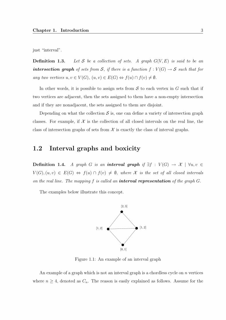
Definition 1.4. A graph G is an interval graph if ∃f : V (G) → X | ∀u, v ∈V (G), (u, v) ∈ E(G) ⇔ f(u) ∩ f(v) 6= ∅, where X is the set of all closed intervals

on the real line. The mapping f is called an interval representation of the graph G.

The examples below illustrate this concept.

[2, 3]

[1, 2][1, 2]

[0, 1]

Figure 1.1: An example of an interval graph

An example of a graph which is not an interval graph is a chordless cycle on n vertices

where n ≥ 4, denoted as Cn. The reason is easily explained as follows. Assume for the


sake of contradiction that Cn is indeed an interval graph. Then, there should exist an

interval representation, say f , for Cn. Let x be the vertex in Cn whose interval has

the leftmost left end-point. Let the cycle be xv1v2 . . . vn−1x. Since (x, v2) is not an

edge, the intervals f(x) and f(v2) are disjoint and since f(x) is the interval with the

leftmost left end-point, we have r(f(x)) < l(f(v2)). For the same reason, we also have

r(f(x)) < l(f(vn−2)) (note that v2 and vn−2 could be the same vertex if n = 4). It is

easy to see that the interval of any vertex that is adjacent to both x and v2 or to both

x and vn−2 will contain the point r(f(x)). Thus both the intervals f(v1) and f(vn−1)

contain the point r(f(x)) implying that f(v1) ∩ f(vn−1) 6= ∅. But (v1, vn−1) is not an

edge in Cn thus contradicting our assumption that Cn is an interval graph.

A cycle C in a graph G is an induced cycle if the subgraph induced by the vertices

of C in G is C. In other words, the induced cycles in a graph are exactly the chordless

cycles in that graph. Since any induced subgraph of an interval graph is also an interval

graph, interval graphs cannot contain induced cycles of length more than 3.

Definition 1.5. A graph G is a chordal graph if there are no induced cycles of length

more than 3 in it.

Interval graphs are thus a subclass of chordal graphs. But not all chordal graphs are

interval graphs. Shown in Figure 1.2 is a graph that has no cycles (and hence is chordal)

but is still not an interval graph.

v1

v2

v3

v4v6

v5

v0

Figure 1.2: v2, v4 and v6 form an asteroidal triple

An asteroidal triple (or AT in short) in a graph is an independent set of three vertices


such that between any two of these vertices, there is a path in the graph that does not

pass through any neighbour of the third vertex. It can be shown that an interval graph

cannot contain an AT. Suppose G is an interval graph and the vertices x, y and z form an

asteroidal triple in G. Let f be an interval representation of G. The intervals f(x), f(y)

and f(z) are pairwise disjoint since x, y, z is an independent set. Assume without loss

of generality that the interval f(y) is in between f(x) and f(z). Now, it is not difficult

to convince oneself that any path in G between x and z will contain at least one vertex

v such that f(v) overlaps f(y). This contradicts the fact that x, y, z is an asteroidal

triple in G.

The graph in Figure 1.2 is not an interval graph because the vertices v2, v4 and v6

form an asteroidal triple.

Definition 1.6. A graph G is an AT-free graph if it contains no asteroidal triples.

It turns out that the two concepts of large induced cycles and asteroidal triples are

enough to characterize interval graphs. If a graph does not have induced cycles of length

more than 3 or asteroidal triples in it, then it is an interval graph.

Theorem 1.7 (Lekkerkerker and Boland [43]). A graph is an interval graph if

and only if it is chordal and AT-free.

The reader should note that Definition 1.4 can be changed to use open intervals

instead of closed intervals. It is an easy exercise to prove that the class of intersection

graphs of open intervals on the real line is the same as that of closed intervals and

therefore, a separate treatment of the two is unnecessary.

1.2.1 k-boxes: intervals in higher dimensions

An interval is the collection of all points on the real line between an upper and a lower

bound. How can we generalize this notion to higher dimensional spaces, say to R2, from

the real line? We could look at an ordered pair of intervals of the form (Ix, Iy). Note that

an ordered pair of intervals (Ix, Iy) describes a rectangle in R2 (with its sides parallel

to the axes) as shown in Figure 1.3. In other words, (Ix, Iy) denotes the set Ix × Iy of


points in R2. It is easy to see that given two rectangles A = (A1, A2) and B = (B1, B2),

X

Iy

Y

Iz

XIx

Iy

Y

B = (Ix, Iy) B = (Ix, Iy, Iz)

Ix

Z

Figure 1.3: A 2-box in R2 and a 3-box in R

3

A ∩ B 6= ∅ (i.e., the two rectangles have at least one point in common) if and only if if

there is an overlap between intervals A1 and B1 (on the X-axis) and between intervals

A2 and B2 (on the Y -axis). We call these rectangles 2-boxes, in the sense that they are

boxes in the 2-dimensional plane R2.

We can generalize this definition to k dimensions by defining the notion of a k-box.

Definition 1.8. A k-box, denoted as a k-tuple of intervals (R1, R2, . . . , Rk) is the set

of points R1 ×R2 × · · · ×Rk.

A k-box could be thought of as a “k-dimensional box” or a “box” in Rk with its sides

parallel to the axes. We sometimes refer to such boxes as “axis-parallel k-dimensional

boxes”. Given two k-boxes A = (A1, . . . , Ak) and B = (B1, . . . , Bk), A ∩ B 6= ∅ ⇔∀i | 1 ≤ i ≤ k, Ai ∩Bi 6= ∅.

Since a k-box denoted by a k-tuple of intervals, X k denotes the set of all k-boxes.

A graph G is said to be an intersection graph of k-boxes if there exists a mapping

f : V (G) → X k such that (u, v) ∈ E(G) ⇔ f(u) ∩ f(v) 6= ∅. Such a mapping f is called

a k-box representation of G. Let us denote by Hk, the class of intersection graphs of k-

boxes, or in other words, the class of graphs that have k-box representations. If a graph

G ∈ Hk, we say that G is “representable” or “can be represented” as the intersection of


k-boxes. By our definition of a k-box, a 1-box is just an interval on the real line. Thus,

H1 is exactly the class of interval graphs. Further, it can be easily seen that for j > i,

Hi ⊆ Hj. This is because if a graph G has an i-box representation f , then it also has

a j-box representation g which can be defined as follows: for every vertex u ∈ V (G),

g(u) is obtained by appending an arbitrary interval I, (j − i) times to the i-tuple f(u).

Thus, if f(u) = (f1(u), . . . , fi(u)), then g(u) = (f1(u), . . . , fi(u), I1, I2, . . . , Ij−i) where

I1 = I2 = · · · = Ij−i = I and I is an arbitrary interval.

But does using higher dimensional boxes give us more power? Do more graphs become

representable as the intersection of k-boxes as we increase k? Let us consider the class

of intersection graphs of 2-boxes. The graph C4, that was observed to be not an interval

graph can be seen to be an intersection graph of 2-boxes (see Figure 1.4). This example

v1

v3

v4v2

v1

v2

v3

v4

Figure 1.4: A 2-box representation for C4

shows that H1 ⊂ H2.

1.2.2 Boxicity

We are now ready to define the parameter boxicity of a graph.

Definition 1.9. The boxicity of a graph G, denoted as box(G), is the minimum

positive integer k such that G is representable as the intersection of k-boxes.

Thus, G is an interval graph if and only if box(G) = 1. Also, since C4 is not an

interval graph but has a 2-box representation as we have seen above, box(C4) = 2.


The natural question to ask now is how high can the boxicity of a graph be? Will it

even be finite? It can be easily shown that if G is any graph on n vertices, box(G) ≤ n.

In fact, a slightly more careful analysis shows that box(G) ≤ ⌊n/2⌋ for any graph G on

n vertices. Roberts [51] has shown that a complete n/2-partite graph with 2 vertices in

each part has boxicity equal to n/2. This graph, which we call the Roberts’ graph on n

vertices is just a complete graph on n vertices with a maximum matching removed from

it. This also shows that for any k ∈ N, and k ≥ 1, there exists a graph with boxicity

equal to k, namely the Roberts’ graph on 2k vertices. It can thus be concluded that for

any k, Hk ⊂ Hk+1 since the Roberts’ graph on 2(k + 1) vertices is in Hk+1 but not in

Hk.

1.2.3 Interval graph representation of a graph

Below, we state a very useful lemma due to Roberts [51].

Lemma 1.10 (Roberts [51]). For any graph G, box(G) ≤ k if and only if there exists

k interval graphs I1, . . . , Ik such that G = I1 ∩ · · · ∩ Ik.Proof:

(⇒): If box(G) ≤ k then there exists a function f : V (G) → X k such that for

any u, v ∈ V (G), (u, v) ∈ E(G) ⇔ f(u) ∩ f(v) 6= ∅. Define functions f1, . . . , fk on

V (G) as follows: for u ∈ V (G), f(u) = (f1(u), . . . , fk(u)). For 1 ≤ i ≤ k, let Ii be an

interval graph with vertex V (G) and interval representation fi. Now, (u, v) ∈ E(G) ⇔f(u) ∩ f(v) 6= ∅ ⇔ ∀i, fi(u) ∩ fi(v) 6= ∅ ⇔ ∀i, (u, v) ∈ E(Ii). It now follows that

G = I1 ∩ · · · ∩ Ik.

(⇐): Let G = I1 ∩ · · · ∩ Ik. For 1 ≤ i ≤ k, let fi : V (G) → X be an interval

representation for Ii (recall that V (Ii) = V (G)). Define f : V (G) → X k as follows:

for u ∈ V (G), f(u) = (f1(u), . . . , fk(u)). We claim that f is a k-box representation for

G. Since G = I1 ∩ · · · ∩ Ik, (u, v) ∈ E(G) ⇔ ∀i, (u, v) ∈ E(Ii) ⇔ ∀i, fi(u) ∩ fi(v) 6=∅ ⇔ f(u) ∩ f(v) 6= ∅. f is therefore a k-box representation for G thus proving that

box(G) ≤ k.


Note that the interval graphs I1, . . . , Ik are supergraphs of G. Thus, the forward

implication of the lemma means that if box(G) ≤ k, then it is possible to find k interval

supergraphs of G such that every edge that is not present in G is not present in at least

one of these interval supergraphs. Conversely, if one can find k interval graphs I1, . . . , Ik

such that G = I1 ∩ · · · ∩ Ik, then box(G) ≤ k. Given below is a straightforward corollary

of Lemma 1.10.

Corollary 1.11. If G = G1 ∩G2 ∩ · · · ∩Gk, then box(G) ≤ ∑ki=1 box(Gi).

Definition 1.12. A collection of interval graphs such that their intersection gives the

graph G is said to be an interval graph representation of G.

Almost always, we prove that the boxicity of a given graph G is not more than k

by constructing an interval graph representation of G with k interval graphs. As an

example, we prove a claim that we made earlier.

Theorem 1.13 (Roberts [51]). If G is any graph on n vertices, box(G) ≤ n.

Proof: For u ∈ V (G), let Iu be an interval graph with vertex set V (G) and interval

representation fu given by:

fu(u) = [0, 1],

∀v ∈ N(u), fu(v) = [1, 2], and

∀v 6∈ N(u), fu(v) = [2, 3].

It can be easily verified that Iu | u ∈ V (G) is an interval graph representation of

G with n interval graphs. It now follows from Lemma 1.10 that box(G) ≤ n.

It should be noted that if H is an induced subgraph of G, then box(H) ≤ box(G).

This is because if fG is a k-box representation for G, then one can obtain a k-box

representation fH for H by letting fH = fG|V (H), the restriction of fG to V (H). This

observation also means that the boxicity of any graph is greater than or equal to the

boxicity of any of its induced subgraphs.

When we deal with box representations of graphs, we are free to use boxes of arbitrary

dimensions, that is to say that the boxes assigned to two different vertices need not be


of the same size or shape as long as they are both axis-parallel. It seems worthwhile to

think about more restricted box representations. For example, what if want all the boxes

used in a box representation to have the same size (i.e., the same dimensions)? Can such

a representation in box(G) dimensions be obtained for every graph G? Let us look at

the simplest case first—when box(G) = 1. The question posed above is equivalent to

asking whether for an interval graph G, there exists an interval representation such that

the intervals assigned to each vertex are of the same length (we define the “length” of an

interval [x1, x2] to be x2 − x1). The answer is no, as illustrated by the graph K1,n, also

known as the star graph (shown in Figure 1.5). K1,n is an interval graph as it has an

interval representation as shown in the figure. But some observation can convince the

reader that if n ≥ 3, K1,n cannot have an interval representation in which all the vertices

are assigned intervals of the same length. Some interval graphs (like the one shown in

v1 v2 v3 vn−1 vnvn−2

c

. . .v1

v2

v3

vn

vn−1

vn−2

c

Figure 1.5: K1,n, the star graph with n arms and an interval representation for it

Figure 1.1) do have interval representations that assign intervals of the same length to

each vertex. As we see in the next section, the class of such interval graphs are called

unit interval graphs, proper interval graphs or indifference graphs.

1.3 Unit interval graphs and cubicity

Now, if we let X1 ⊂ X to be the set of all unit length intervals on the real line, the class

of intersection graphs on X1 is the class of unit interval graphs or indifference graphs.


Definition 1.14. A graph G is a unit interval graph if ∃f : V (G) → X1 | ∀u, v ∈V (G), (u, v) ∈ E(G) ⇔ f(u) ∩ f(v) 6= ∅, where X1 is the set of all closed intervals of

length 1 on the real line. The mapping f is called a unit interval representation of

the graph G.

For x ∈ R+, let Xx denote the set of all closed intervals of length x on the real line. If

a graph G has a unit interval representation f , then for any x ∈ R+ it also has an interval

representation g : V (G) → Xx defined as: ∀u ∈ V (G), g(u) = [x · l(f(u)), x · r(f(u))].

Clearly, g is an interval representation for G that maps the vertices in G to intervals of

length x. g is thus an equal interval representation as defined below.

Definition 1.15. An interval representation f of a graph G is called an equal interval

representation with interval length x if for each v ∈ V (G), r(f(v)) − l(f(v)) = x.

Conversely, if a graph G has an equal interval representation g with interval length x

(where x ∈ R+), then it has a unit interval representation f given by: ∀u ∈ V (G), f(u) =

[

1x· l(g(u)), 1

x· r(g(u))

]

. It can thus be seen that unit interval graphs are exactly those

graphs with equal interval representations.

Note that the class of unit interval graphs is also exactly the class of interval graphs

which have an interval representation such that the interval assigned to no vertex is

properly contained in the interval assigned to another vertex as shown in [32]. Therefore,

these graphs are also called proper interval graphs.

1.3.1 Unit and equal interval representations as mappings to

real numbers

Since a unit length interval is completely specfied by just one of its end-points, a unit

interval representation could assign just real numbers (instead of unit length intervals)

to vertices in such a way that two vertices are adjacent if and only if the real numbers

assigned to them differ by at most 1. Note that we could think of these real numbers

as the left end-points of the unit intervals assigned to the vertices. The same is true

for equal interval representations of interval length x. In this case, two vertices are


adjacent if and only if the real numbers assigned to them differ by at most x. This

idea can be expressed mathematically as follows. If f is an equal interval representation

with interval length x for the unit interval graph G, then define g : V (G) → R as: for

u ∈ V (G), g(u) = l(f(u)). Now, (u, v) ∈ E(G) ⇔ f(u) ∩ f(v) 6= ∅ ⇔ |g(u) − g(v)| ≤ x.

Conversely, if g is a function that maps the vertices of G to real numbers such that

(u, v) ∈ E(G) ⇔ |g(u) − g(v)| ≤ x for some x ∈ R+, then we can define a function

f : V (G) → Xx as: for u ∈ V (G), f(u) = [g(u), g(u) + x]. We therefore have (u, v) ∈E(G) ⇔ |g(u) − g(v)| ≤ x ⇔ f(u) ∩ f(v) 6= ∅. We implicitly assume the existence of

f when we speak of g and therefore we do not make any distinction between f and g.

Thus, we say that g is an equal interval representation with interval length x for G and

if x = 1, we say that g is a unit interval representation for G. We thus have the following

alternate definition for unit and equal interval representations.

Definition 1.16. Given a graph G, a function f : V (G) → R such that (u, v) ∈ E(G) ⇔|f(u)− f(v)| ≤ x is called an equal interval representation with interval length x of

the graph G. If x = 1, then we call f a unit interval representation of G.

1.3.2 k-cubes

Recall that we generalized intervals on the real line to k-boxes in Rk. Along the same

lines, we define a k-cube as follows.

Definition 1.17. A k-cube, denoted as (R1, R2, . . . , Rk), where each Ri is a unit

length interval on the real line, is the set of points R1 ×R2 × · · · ×Rk.

k-cubes are also referred to as “axis-parallel k-dimensional cubes”. Since a k-cube

is denoted by a k-tuple of unit length intervals, it can be thought to be a member

of the set (X1)k. As we saw in the last paragraph, each Ri, being a unit interval, is

completely defined by just specifying its left end-point l(Ri), since r(Ri) = l(Ri) + 1.

Thus the k-cube (R1, R2, . . . , Rk) can be alternately denoted by a k-tuple of real numbers

(l(R1), l(R2), . . . , l(Rk)). This notation allows us to think of k-cubes as members of Rk


and often makes their handling easier. If A,B ∈ Rk are two k-cubes such that A =

(a1, . . . , ak) and B = (b1, . . . , bk), then A ∩B 6= ∅ if and only if for each i, |ai − bi| ≤ 1.

A graph G is said to be an intersection graph of k-cubes if ∃f : V (G) → Rk, such

that (u, v) ∈ E(G) ⇔ f(u) ∩ f(v) 6= ∅ or in other words, there exists a mapping f that

maps the vertices of G to k-cubes such that two vertices u and v in G are adjacent if

and only if the k-cubes corresponding to them have a non-empty intersection. Such a

mapping f is called a k-cube representation of G.

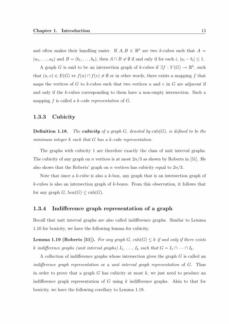
1.3.3 Cubicity

Definition 1.18. The cubicity of a graph G, denoted by cub(G), is defined to be the

minimum integer k such that G has a k-cube representation.

The graphs with cubicity 1 are therefore exactly the class of unit interval graphs.

The cubicity of any graph on n vertices is at most 2n/3 as shown by Roberts in [51]. He

also shows that the Roberts’ graph on n vertices has cubicity equal to 2n/3.

Note that since a k-cube is also a k-box, any graph that is an intersection graph of

k-cubes is also an intersection graph of k-boxes. From this observation, it follows that

for any graph G, box(G) ≤ cub(G).

1.3.4 Indifference graph representation of a graph

Recall that unit interval graphs are also called indifference graphs. Similar to Lemma

1.10 for boxicity, we have the following lemma for cubicity.

Lemma 1.19 (Roberts [51]). For any graph G, cub(G) ≤ k if and only if there exists

k indifference graphs (unit interval graphs) I1, . . . , Ik such that G = I1 ∩ · · · ∩ Ik.A collection of indifference graphs whose intersection gives the graph G is called an

indifference graph representation or a unit interval graph representation of G. Thus

in order to prove that a graph G has cubicity at most k, we just need to produce an

indifference graph representation of G using k indifference graphs. Akin to that for

boxicity, we have the following corollary to Lemma 1.19.


Corollary 1.20. If G = G1 ∩G2 ∩ · · · ∩Gk, then cub(G) ≤ ∑ki=1 cub(Gi).

1.4 A note on the asymptotic notation

We use the asymptotic notation to express various bounds on the boxicity and cubicity

of graphs. A short description of the way in which we use the asymptotic notation is

given below.

Let ℘(G) be a graph parameter such as box(G) or cub(G) and let f(G) be a function

that is defined in terms of various parameters of G. We denote by “℘(G) = O(f)” or

“℘(G) ∈ O(f)” or “℘ is O(f)” the fact that there exists constants c0 and c such that

for any graph G, ℘(G) ≤ c0 + cf(G). For example, in Chapter 4, we prove that for

any graph G on n vertices and having maximum degree ∆, cub(G) ≤ ⌈4(∆ + 1) lnn⌉.Because of this result, we say that cub(G) is O(∆ lnn).

Similarly, by “℘(G) = Ω(f)” or “℘(G) ∈ Ω(f)” or “℘ is Ω(f)” we mean that there

exist constants c0 and c such that f(G) ≤ c0 + c℘(G). “℘(G) = Θ(f)” denotes the fact

that ℘(G) = O(f) and ℘(G) = Ω(f).

1.5 A short survey of previous literature

The parameters boxicity and cubicity of graphs were introduced by F. S. Roberts [51] in

1969. Roberts showed that for any graph G on n vertices box(G) ≤ n/2 and cub(G) ≤2n/3. Both these bounds are tight since box(K2,2,...,2) = n/2 and cub(K3,3,...,3) = 2n/3

where K2,2,...,2 denotes the complete n/2-partite graph with 2 vertices in each part and

K3,3,...,3 denotes the complete n/3-partite graph with 3 vertices in each part.

It is easy to see that the boxicity of any graph is at least the boxicity of any induced

subgraph of it.


1.5.1 Results on boxicity

It was shown by Cozzens [23] that computing the boxicity of a graph is NP-hard. This

was later improved by Yannakakis [62], and finally by Kratochvıl [40] who showed that

deciding whether the boxicity of a graph is at most 2 itself is NP-complete.

In many algorithmic problems related to graphs, the availability of certain convenient

representations turns out to be extremely useful. Probably, the most well-known and

important examples are the tree decompositions and path decompositions [7]. Many

NP-hard problems are known to be polynomial time solvable given a tree(path) decom-

position of bounded width for the input graph. Similarly, the representation of graphs

as intersections of “disks” or “spheres” lies at the core of solving problems related to

frequency assignments in radio networks, computing molecular conformations etc. For

the maximum independent set problem which is hard to approximate within a factor

of n(1/2)−ǫ for general graphs [35], a PTAS is known for disk graphs given the disk rep-

resentation [27, 13]. In a similar way, the availability of a box representation in low

dimension makes some well known NP hard problems polynomial time solvable. For

example, it was shown in [53] that the max-clique problem is polynomial time solvable

in graph classes with a polynomial bound on the number of maximal cliques. Since

boxicity k graphs have only O((2n)k) maximal cliques, the max-clique problem admits

a polynomial-time algorithm in bounded boxicity graphs. It was shown in [35] that the

complexity of finding the maximum independent set is hard to approximate within a

factor n(1/2)−ǫ for general graphs. In fact, [35] gives the stronger inapproximability result

of n1−ǫ, for any ǫ > 0, under the assumption that NP6=ZPP. Though this problem is

NP-hard even for boxicity 2 graphs, it is approximable to a factor of ⌊1 + 1c

log n⌋d−1 for

any constant c ≥ 1 for boxicity d (d ≥ 2) graphs given a box representation [2, 5]. It was

shown in [16] that for any graph G, box(G) ≤ tw(G) + 2, where tw(G) is the treewidth

of G. This result implies that the class of ‘low boxicity’ graphs properly contains the

class of ‘low treewidth graphs’.

Researchers have also tried to bound the boxicity of graph classes with special struc-

ture. Scheinerman [54] showed that the boxicity of outer planar graphs is at most 2.


Thomassen [57] proved that the boxicity of planar graphs is bounded above by 3. Upper

bounds for the boxicity of many other graph classes such as chordal graphs, AT-free

graphs, permutation graphs etc. were shown in [16] by relating the boxicity of a graph

with its treewidth. Researchers have also tried to generalize or extend the concept of box-

icity in various ways. The poset boxicity [59], the rectangle number [20], grid dimension

[4], circular dimension [30, 55] and the boxicity of digraphs [19] are some examples.

1.5.2 Boxicity in other scientific disciplines

Box representations of graphs find application in problems from ecology and operations

research. As an example, we give an outline of a problem from ecology below:

Niche problem in ecology:

Ecologists study the interactions between various organisms in an environment. Each

species has a natural habitat in which it is commonly found. If we examine different

environmental factors like temperature, humidity, pH etc. of the natural habitats of a

species, we can find for each factor a range of values which characterizes the habitats

in which the species is found. If we have k such factors, we can define a k-dimensional

space with an axis for each such factor. Such a space is called the “ecological phase

space”. The range of values of each factor for a species together defines a k-box, or

the “ecological niche” of the species. If the ecological niches of two species overlap,

then they can be together found in some habitats. Ecologists traditionally use directed

graphs called “food webs” which define the “predator-prey” relationship between a set

of species. There is an edge from a species X to a species Y in this graph if Y preys on

X. Now, two species compete for food if they have a common prey. An undirected graph

drawn with the vertex set as a set of species and with edges in such a way that there is

an edge between two species if they have a common prey is called a “competition graph”.

An edge in this graph between two species X and Y means that X and Y compete for

food. At the same time, considering an ecological phase space in which one dimension

is the “feeding dimension” (an axis with the kinds of food that various species eat along


it), two species compete if and only if their ecological niches in this phase space overlap.

Now, if we have a competition graph of a set of species from various sources of data like

food webs, then the question of what the boxicity of the graph is becomes interesting.

This problem was studied extensively by Cohen [21]. He observed that in most cases,

the competition graphs turn out to be interval graphs which means that one dimension

suffices to explain the competition graph. Considering that a large majority of possible

graphs are not interval graphs, this seems too much of a coincidence. Roberts gives a

nice overview of this problem in [52].

1.5.3 Results on cubicity

It has been shown that deciding whether the cubicity of a given graph is at least 3 is

NP-hard [62].

It is easy to see that the problem of representing graphs using k-cubes can be equiv-

alently formulated as the following geometric embedding problem. Given an undirected

unweighted graph G = (V,E) and a threshold t, find an embedding f : V → Rk of the

vertices of G into a k-dimensional space (for the minimum possible k) such that for any

two vertices u and v of G, ||f(u) − f(v)||∞ ≤ t if and only if u and v are adjacent. The

norm || ||∞ is the L∞ norm. Clearly, a k-cube representation of G yields the required

embedding of G in the k-dimensional space. The minimum dimension required to embed

G as above under the L2 norm is called the sphericity of G. Refer to [47] for applications

where such an embedding under L∞ norm is argued to be more appropriate than em-

bedding under L2 norm. The connection between cubicity and sphericity of graphs were

studied in [31, 45]. The cube representation of special classes of graphs like hypercubes

and complete multipartite graphs were investigated in [51, 45, 48]. Also, the cubicity of

the d-dimensional hypercube was shown to be Θ( dlog d

) in [17]. A lower bound for the

cubicity of general graphs in terms of the diameter and maximum independent set size

was shown in [14].

The ratio of cubicity to boxicity of any graph on n vertices was shown to be at most

⌈log2 n⌉ in [15].


1.5.4 Other geometric intersection graph classes

Like interval and unit interval graphs, a number of classes of geometric intersection

graphs have been studied. Circular arc graphs [32] are the intersection graphs of arcs

on a circle and circle graphs are the intersection graphs of chords of a circle. Tolerance

graphs [33] generalize interval graphs to allow a restricted overlap between two intervals.

An intersection model for permutation graphs is given [32]. Trapezoid graphs are the

intersection graphs of trapezoids between two parallel lines [25]. Graphs defined as the

intersection of a number of different kinds of geometric objects in the plane are described

in [40].

Interval catch digraphs [49] have an intersection model very similar to that of interval

graphs but are directed graphs. In this model, a pair (Ix, px), where Ix is an interval and

px is a point in Ix, is assigned to each vertex such that there is a directed edge (x, y) in

the graph if and only if py ∈ Ix.

Another generalization of interval graphs is to make the set assigned to each vertex

the union of k intervals such that two vertices are adjacent if and only if the sets assigned

to them have a non-empty intersection. The minimum k required to represent a graph

in such a way is called its interval number [58].

A survey of a number of intersection graph classes and their applications is available

in [46].

1.6 Outline of the rest of the thesis

Chapter 2 investigates the relationship between the maximum degree and the boxicity

of a graph. The previous upper bound for boxicity in terms of the maximum degree ∆

of a graph was ⌈(∆ + 2) lnn⌉ 1. A new upper bound of 2∆2 for boxicity is presented,

thereby showing that the boxicity of a bounded degree graph is bounded no matter how

large the graph is.

1Note that almost invariably, we use n to denote the number of vertices of the graph under

consideration.


Chapter 3 shows that even though there are graphs whose boxicity is not O(dav lnn)

where dav is the average degree, such graphs are rare. The theory of random graphs is

used to show that in a suitable random graph model, the probability of the randomly

drawn graph to have a boxicity that is O(dav lnn) goes to 1 as n becomes large. We

make use of the upper bound on boxicity proved in Chapter 2 to prove this result.

In Chapter 4, we see that if we randomly generate ⌈4(∆ + 1) lnn⌉ indifference su-

pergraphs of an input graph G, then there is a slight possibility that these indifference

graphs form an indifference graph representation of G. Thus we have an upper bound of

⌈4(∆ + 1) lnn⌉ on the cubicity of a graph. The randomized algorithm is derandomized

to obtain a deterministic polynomial-time algorithm that outputs a cube representation

of the input graph in ⌈4(∆ + 1) lnn⌉ dimensions.

Two results relating the cubicity and the bandwidth of a graph are presented in

Chapter 5. A bandwidth ordering of the graph is taken as input and the construction

introduced in Chapter 4 is applied to show an O(∆ ln b) upper bound for the cubicity of

any graph with maximum degree ∆ and bandwidth b. Another upper bound of b+ 1 on

the cubicity is also shown. This bound is used to show upper bounds on the cubicity of

circular-arc graphs, cocomparability graphs and AT-free graphs.

Each of Chapters 6–8 deals with a special graph class.

The upper bound of b+1 for cubicity automatically gives us an upper bound of ∆+1

for the cubicity of any interval graph. In Chapter 6, we show that a much tighter upper

bound of ⌈log2 ∆⌉ + 4 exists for the cubicity of interval graphs.

Outerplanar graphs are studied next. As mentioned before, it was proved by Schein-

erman [54] that outerplanar graphs need boxicity at most 2. Chapter 7 gives an inde-

pendent proof that shows the same result.

In Chapter 8, we look at Halin graphs, which are a restricted class of planar graphs

incomparable with the class of outerplanar graphs. We show that every Halin graph that

is not a K4 has boxicity equal to 2.

Chapter 2

Upper bounds for boxicity

Roberts gave us an upper bound of n/2 for the boxicity of any graph on n vertices. We

shall now try to derive a different upper bound for boxicity in terms of the maximum

degree ∆ of the graph.

2.1 Previous upper bounds on boxicity

2.1.1 Boxicity is O(∆ lnn)

Lemma 1.10 tells us that the boxicity of a graph G is the minimum number of interval

supergraphs of G such that each non-edge (or “missing edge”) in G is a non-edge in at

least one of these interval supergraphs. One could try to devise some method by which

we can obtain supergraphs of G in such a way that each missing edge in G is missing

in one of these supergraphs. Of course, one could obtain supergraphs of G by adding

arbitrary sets of edges to G. But the catch is that we need only those supergraphs of G

that are also interval graphs. It seems difficult to systematically generate supergraphs

of G that are also interval graphs. In [18], Chandran and Sivadasan try to generate

interval supergraphs of G at random and come up with a simple randomized algorithm

that generates an interval graph representation of the input graph G on n vertices and

with maximum degree ∆ using ⌈(∆ + 1) lnn⌉ interval graphs with non-zero probability.

The existence of this algorithm proves the following theorem.

21

Chapter 2. Upper bounds for boxicity 22

Theorem 2.1 (Chandran and Sivadasan). Given a graph G on n vertices with

maximum degree ∆, box(G) ≤ ⌈(∆ + 2) lnn⌉.In Chapter 4, we extend this randomized construction to show that a similar upper

bound exists for cubicity.

2.1.2 Boxicity and average degree

The relationship between the boxicity of a graph and its average degree is also explored

in [18]. It is shown that in general the boxicity of a graph on n vertices with average

degree dav is not O(dav lnn) as there exist graphs with boxicity that is exponentially

larger than dav lnn. In Chapter 3, we show that even though such graphs exist, for most

graphs, boxicity is O(dav lnn).

2.2 Boxicity of bounded degree graphs

If the family of graphs under consideration has bounded degree, the upper bound of

⌈(∆ + 2) lnn⌉ for the boxicity is an improvement over previous bounds as it implies that

boxicity of graphs in that family is O(lnn). But is this the best possible for bounded

degree graphs? No matter what graph we take, it seems that the boxicity is always less

than or equal to ∆. Might it be the case that the boxicity of any graph with maximum

degree ∆ is O(∆)? The anwer to that question certainly does not appear to be easy. We

could first try and see if boxicity can be bounded from above by a function of ∆ alone.

Such an upper bound would be interesting as it would mean that the boxicity of graphs

with bounded degree—like expander graphs—is bounded no matter how large the graph

is. We shall now look at a simple proof that shows that boxicity is in fact O(∆2).

In order to avoid confusion, we shall use ∆(G) to denote the maximum degree of a

graph G for the remainder of this section. We shall show that for any graph G with

maximum degree ∆(G), box(G) ≤ 2∆(G)2. Let χ(G) denote the chromatic number of

G. We use Brooks’ theorem, which states that χ(G) ≤ ∆(G) for any connected graph G

unless it is an odd cycle or a complete graph. We also use the square G2 of a graph G,


defined to be the graph obtained from G by adding edges joining nonadjacent vertices

that have a common neighbour in G. Note that since any vertex will become adjacent

to at most ∆(G) (∆(G) − 1) new vertices when the graph is squared, ∆(G2) ≤ ∆(G)2.

If G = G1∩G2∩· · ·∩Gk, then by Corollary 1.11, box(G1∩· · ·∩Gk) ≤ ∑ki=1 box(Gi);

we will use this fact.

Theorem 2.2. If G is a graph with ∆(G) = D, then box(G) ≤ 2D2.

Proof: Let n = |V (G)|. Let k = χ(G2), and let c be a proper k-coloring ofG2 using colors

1, . . . , k. For 1 ≤ i ≤ k, let Vi = u ∈ V (G) : c(u) = i (recall that V (G2) = V (G)). For

1 ≤ i ≤ k, let Hi be the complete graph with vertex set V (G) − Vi, and let Gi be the

graph with V (Gi) = V (G) and E(Gi) = E(G) ∪ E(Hi).

Consider vertices u and v. If they are adjacent in G, then they are adjacent in each

Gi, since E(G) ⊆ E(Gi). If they are not adjacent in G, then they are nonadjacent in

both Gc(u) and Gc(v). Hence G = G1 ∩ · · · ∩ Gk. Note that G2 will contain a triangle

if there is a vertex with degree 2 or more in G. Therefore, it is clear that G2 cannot

be an odd cycle except when n = 3, in which case it is a complete graph. If G2 is a

complete graph, we have D2 ≥ ∆(G2) = n−1 and therefore, box(G) ≤ 2D2 (because we

know that box(G) ≤ n/2). Thus, by Brooks’ theorem, we can assume that k = χ(G2) ≤∆(G2) ≤ D2. Now, it suffices to show that box(Gi) ≤ 2 for each i.

· · ·Vi

V − Vi

= Gi

Figure 2.1: Structure of Gi: the two dotted edges cannot be both present


If x, y ∈ Vi (i.e., c(x) = c(y) = i) and (x,w), (y, w) ∈ E(G) for some w ∈ V (G), then

(x, y) ∈ E(G2), which prevents c(x) = c(y). Hence in G, each vertex outside Vi has at

most one neighbour in Vi (see Figure 2.1). By construction, the edges of Gi incident to

Vi are edges of G. Hence in Gi each vertex outside Vi has at most one neighbour in Vi.

To obtain box(Gi) ≤ 2, we define interval graphs I and I ′ on V (G) whose intersection

is Gi. Let Vi = v1, . . . , vh. In both I and I ′, assign the single-point interval j to vj.

Consider w ∈ V (G) − Vi. If w has no neighbour in Vi, then assign w the single-point

intervals 0 in I and n in I ′. If w has neighbour vj ∈ Vi (there can only be one such

neighbour, as noted before), then assign w the intervals [0, j] in I and [j, n] in I ′. By

construction, E(Gi) ⊆ E(I) ∩ E(I ′).

It remains to show that nonadjacent vertices in Gi are nonadjacent in I or I ′. All

nonadjacent pairs in Gi include a vertex of Vi; consider vj ∈ Vi. Let (vj, w) be the

nonadjacent pair. Note that Vi is independent in both I and I ′. Thus, we can assume

that w ∈ V (G) − Vi. Then either the interval for w in I ends before the point j, or the

interval for w in I ′ begins after the point j.

2.3 Concluding remarks

We have seen that the availability of a low dimensional box representation for a graph

can lead to polynomial time algorithms and to better approximation ratios for NP-hard

problems. Thus, it is interesting to design efficient algorithms to represent graphs of

small boxicity in a small number of dimensions. Theorem 2.2 gives an upper bound

for boxicity in terms of the maximum degree ∆ alone. This means that no matter how

large a graph might be, a box representation in a small number of dimensions can be

constructed for it if it has a small maximum degree.

Most bounds on boxicity show that box(G) is small when the complement of G is

small or sparse (for example, box(G) is bounded by the minimum size of a maximal

matching in the complement; see [24]). This upper bound is perhaps the first general

bound showing that box(G) is small when G itself is small. We do not claim that this


upper bound is optimal; but make the following conjecture instead.

Conjecture. For any graph G with maximum degree ∆, box(G) is O(∆).

Roberts’ graphs are a family of graphs that have boxicity Ω(∆). In fact, we do not

know of any graph that has boxicity greater than its maximum degree.

Since box(G) ≤ n/2 when G has n vertices (as shown in [51]), the upper bound

provided by Theorem 2.2 is of no use when ∆ >√n/2. Since for any graph G on n

vertices with maximum degree ∆, box(G) ≤ ⌈(∆ + 2) lnn⌉ as shown by Theorem 2.1,

the bound of 2∆2 given by Theorem 2.2 is better only when ∆ ≤ lnn.

We are now armed with two upper bounds for the boxicity of general graphs in terms

of the maximum degree. Both these bounds come in handy in the next chapter when we

look at the boxicity of random graphs. As mentioned in Section 2.1.2, there are families

of graphs for which the boxicity is exponentially larger than dav lnn, but we now exploit

the power of probabilistic techniques to show that such graphs are rare.

Chapter 3

Boxicity of random graphs

Though an O(dav lnn) upper bound does not exist for boxicity of a general graph on

n vertices with average degree dav, we now show that for almost all graphs, there does

exist an upper bound for boxicity that is O(dav lnn). First, we shall look at some basics

of the theory of random graphs.

3.1 Random graph preliminaries

Often, it is informative to look at graph properties from a statistical viewpoint. We

could ask such questions as “if a graph is randomly drawn from a collection of graphs,

what is the probability that the randomly chosen graph has property P?”. In order to

answer such questions, we need to define a probability space of graphs (we consider only

finite graphs here) from which we draw a graph at random. The two most popularly

used probability distributions (also called random graph models) are:

• The G(n, p) model: This is a probability space of all graphs on n vertices. The

act of drawing a graph at random from this model is defined by the following

random experiment. Toss a coin that turns up heads with probability p for each

of the(

n2

)

possible edges. If the coin turns up heads, then we decide that the

particular edge is present in the randomly drawn graph and the edge is not present

otherwise. Thus, each edge has an independent probability of p of being present

27

Chapter 3. Boxicity of random graphs 28

in the randomly drawn graph. Clearly, this is not a uniform distribution over all

graphs on n vertices. The probability of a graph with m edges to be the randomly

drawn graph is pm(1 − p)(n2)−m. Note that the distribution becomes uniform if

p = 12.

• The G(n,m) model: In this model, the randomly chosen graph is drawn uniformly

at random from the collection of all graphs on n vertices with m edges. Thus the

probability of any given graph on n vertices and m edges to occur as the randomly

chosen graph is the same, i.e. 1/(

Nm

)

where N =(

n2

)

.

We say that a given property P is true for almost all graphs if for a randomly chosen

graph G from the random graph model under consideration, Pr[G has property P ] → 1

when n → ∞. This can be seen as the mathematical way of saying that the proportion

of graphs without property P becomes negligibly small as n becomes large and therefore

“almost all” graphs can be thought to have this property.

3.2 Boxicity is O(dav lnn) for almost all graphs

The proof shows that for almost all graphs G drawn from the G(n,m) model, box(G) ∈O(c lnn) where c = 2m/n (refer to Section 1.4 for a description of the asymptotic

notation as we use it). We assume c > 1 as we are mainly interested in connected

graphs. But we first show the result for the G(n, p) model setting p = c/(n − 1). As

shown in [9], we can then carry over the result to the G(n,m) model since p = m/(

n2

)

.

Consider the G(n, p) model with p = c/(n− 1). Let G denote a random graph drawn

according to this model. For a vertex u, define a random variable du that denotes the

degree of u, i.e. du = |N(u)| =∑

v∈V (G),v 6=u eu,v where eu,v is an indicator random variable

whose value is 1 if (u, v) ∈ E(G) and 0 otherwise. Therefore, E[du] = p(n− 1) = c.

Case 1: c ≥ lnn.

Since du is the sum of independent Bernoulli random variables, we can use Chernoff

bound to bound the probability of du becoming large. In particular, we use the following


form of the Chernoff bound given in [3] for the rest of the proof.

Pr[X ≥ (1 + δ)E[X]] ≤ e−δ2E[X]2+δ (3.1)

for all δ > 1. Taking δ = 5, we get, Pr[du ≥ 6c] ≤ 1/n3. Now, by the union

bound, it follows that Pr[∆(G) ≥ 6c] = Pr[∃u ∈ V (G), du ≥ 6c] ≤ 1/n2. Using the re-

sult box(G) ≤ ⌈(∆ + 2) lnn⌉, we now have, box(G) ≤ (6c + 2) lnn with probability at

least 1 − 1/n2.

Case 2: c < lnn.

Let Su = V (G) −N(u) − u.

Let N ′(u) = v ∈ Su | ∃u′ ∈ N(u) such that (u′, v) ∈ E(G).

In this case, we will use a different technique to upper bound boxicity. Let the graph

G2 denote the square of G. That is, V (G2) = V (G) and (u, v) ∈ E(G2) if there is a path

of length 1 or 2 between u and v. Recall that the proof of Theorem 2.2 shows that for

any graph G, box(G) ≤ 2χ(G2) ≤ 2∆(G2) + 2. We will show below that if c < lnn, then

∆(G2) ≤ c + 6 lnn + 7c2 + 42c lnn, with high probability. The reader may note that

the degree of a vertex u in G2 equals |N(u)| + |N ′(u)|. We will now show that for any

vertex u, Pr[|N(u)| + |N ′(u)| /∈ O(c log n)] ≤ 3/n3.

Let k = c+ 6 lnn. We apply Chernoff bound (3.1) with δ = 6 lnn/c to obtain

Pr[du ≥ k] ≤ e−δ(6 ln n)/(2+δ) ≤ 1/n3

Let A ⊆ V (G) such that |A| < k. Let Z(A) denote the event that N(u) = A. Now, for

each vertex v ∈ Su, let Xv,A denote an indicator random variable indicating whether v ∈N ′(u) conditioned on the event Z(A). Note that for any vertex v ∈ Su, Pr[Xv,A = 1] ≤kp. Let XA =

∑

v∈SuXv,A. It follows that E[XA] ≤ kp(n− 1) = kc. Since XA is the sum

of independent Bernoulli random variables, we apply the Chernoff bound (3.1) by fixing

δ = 6kc/E[XA] to obtain Pr[XA ≥ 7kc] ≤ e−δ(6kc)/(2+δ) ≤ 1/n3.


Let the random variable Xu denote the cardinality of N ′(u). We now have,

Pr[Xu ≥ 7kc | du < k] =∑

A⊆V (G),|A|<k

Pr[(Xu ≥ 7kc) ∧ Z(A)]

=∑

A⊆V (G),|A|<k

Pr[XA ≥ 7kc] Pr[Z(A)] ≤ 1/n3

It follows that

Pr[Xu ≥ 7kc] = Pr[Xu ≥ 7kc | du < k] Pr[du < k]

+Pr[Xu ≥ 7kc | du ≥ k] Pr[du ≥ k]

≤ (1/n3)Pr[du < k] + (1/n3)Pr[Xu ≥ 7kc | du ≥ k] ≤ 2/n3

Let tu = |N(u)|+ |N ′(u)| = du +Xu. Combining the bounds on the values of du and Xu,

we get,

Pr[tu ≥ k + 7kc] ≤ Pr[du ≥ k] + Pr[Xu ≥ 7kc] ≤ 3/n3

Observe that ∆(G2) = maxu∈G tu. Thus, by applying the union bound, we obtain

Pr[

∆(G2) ≥ k + 7kc]

= Pr

∨

u∈V (G)

tu ≥ k + 7kc

≤ 3/n2

Thus, with high probability, ∆(G2) < k + 7kc = c + 6 lnn + 7c2 + 42c lnn. Recalling

that box(G) ≤ 2∆(G2) + 2, we obtain box(G) ∈ O(c lnn) with high probability, since

c < lnn.

Having shown that in the G(n, p) model, Pr[box(G) 6∈ O(c lnn)] ≤ 3/n2, the following

relation from page 35 of [9] helps us to extend our result to the G(n,m) model.

Pm(Q) ≤ 3m1/2Pp(Q)

where Q is a property of graphs of order n, and Pm(Q) and Pp(Q) are the probabilities

of a graph chosen at random from the G(n,m) or the G(n, p) models respectively to have


property Q given that p = m/(

n2

)

. Using this result, we now have, for a graph G drawn

randomly from the G(n,m) model,

Pr[box(G) 6∈ O(c lnn)] ≤ 9n−2√m ≤ 9/n

As c = 2m/n = dav, which is the average degree, we have shown that for almost all

graphs with a given average degree dav, the boxicity is O(dav lnn).

Thus we have the following theorem:

Theorem 3.1. For a random graph G on n vertices and m edges drawn according to

G(n,m) model,

Pr

[

box(G) = O

(

2m

nlnn

)]

≥ 1 − 9

n

3.3 Remarks

We know that box(G) ≤ tw(G) + 2 [16]. It is well known that almost all graphs on n

vertices and m = cn edges (for a sufficiently large constant c) have treewidth Ω(n) [37].

From the discussion in this chapter, we know that almost all graphs on n vertices and m

edges have boxicity O(dav lnn) where dav = 2m/n. An implication of this is that when c

is a large enough constant, for almost all graphs on m = cn edges, there is an exponential

gap between their boxicity and treewidth. Hence it is interesting to reconsider those NP-

hard problems that are polynomial time solvable in bounded treewidth graphs and see

whether they are also polynomial time solvable for bounded boxicity graphs.

Chapter 4

A randomized construction for

cubicity

Let us now turn our attention to the cubicity of graphs. Recall that the cubicity of a

graph is the minimum dimension in which it can be represented as the intersection of

k-cubes. It is immediate that the cubicity of a graph is always at least its boxicity as a

k-cube representation for a graph is also a k-box representation for it.

It seems natural to think about the relationship between the boxicity and cubicity of

a graph. Chandran and K. A. Mathew show in [15] that cub(G)box(G)

≤ ⌈log2 n⌉ for any graph G

on n vertices. In Chapter 2, we saw two upper bounds on the boxicity of any graph G on n

vertices and having maximum degree ∆, namely, box(G) = O(∆ lnn) and box(G) ≤ 2∆2.

Combining these with the result cub(G)box(G)

≤ ⌈log2 n⌉, we get cub(G) = O(∆ ln2 n) and

cub(G) ≤ 2∆2⌈log2 n⌉. In this chapter, we suitably adapt the randomized construction

of [18] to show that cub(G) is O(∆ lnn) which is an improvement over both these bounds

on cubicity.

Let G be a graph on n vertices with maximum degree ∆. We first show a ran-

domized algorithm RAND to construct the cube representation of G in ⌈4(∆ + 1) lnn⌉dimensions. We then give a detailed exposition of the derandomization technique by

demonstrating how the algorithm RAND can be derandomized to obtain a polynomial

time deterministic algorithm DET that gives a cube representation of G in the same

33

Chapter 4. A randomized construction for cubicity 34

number of dimensions. Both these algorithms compute an indifference graph represen-

tation of G using ⌈4(∆ + 1) lnn⌉ indifference graphs. The algorithms construct equal

interval representations (recall the definition from Section 1.3) for each graph in the

indifference graph representation.

4.1 The algorithm RAND

In this section we describe the randomized algorithm RAND that computes a cube

representation in O(∆ lnn) dimensions for any graph G on n vertices and maximum

degree ∆ .

For ease of notation we will let V = V (G) for the remainder of this chapter. The

reader might find it useful to recall the definition of a permutation as given in Definition

1.2.

Definition 4.1. Let π be a permutation of a set S. Let X ⊆ S. The restriction of π

onto X, denoted as πX , is a permutation of X defined as follows. Let X = u1, . . . , ursuch that π(u1) < π(u2) < · · · < π(ur). Then πX(u1) = 1, πX(u2) = 2, . . . , πX(ur) = r.

Construction of the indifference supergraph M(G, π,A):

Let π be a permutation on V and let A be a subset of V . We define M(G, π,A) to be

an indifference graph G′ with V (G′) = V constructed as follows.

Let B = V − A. We shall construct f , an equal interval representation (recall

Definition 1.16) with interval length n for G′ as follows:

∀u ∈ B, define f(u) = n+ π(u),

∀u ∈ A and N(u) ∩B = ∅, define f(u) = 0,

∀u ∈ A and N(u) ∩B 6= ∅, define f(u) = maxx∈N(u)∩B π(x).

Thus, two vertices u and v will have an edge in G′ if and only if |f(u) − f(v)| ≤ n.

Clearly, G′ is an indifference graph. It can be seen that the vertices in B induce a clique

in G′ as the intervals assigned to each of them contain the point 2n. Similarly, all the


vertices in A also induce a clique in G′ as the intervals mapped to each contain the point

n.

Now, we show that G′ is a supergraph of G. To see this, take any edge (u, v) ∈ E(G).

If u and v both belong to A or if both belong to B, then (u, v) ∈ E(G′) as we have

observed above. If this is not the case, then we can assume without loss of generality that

u ∈ A and v ∈ B. Let t = maxx∈N(u)∩B π(x). Obviously, t ≥ π(v), since v ∈ N(u) ∩ B.

From the definition of f , we have f(u) = t and we have f(v) = n + π(v). Therefore,

f(v) − f(u) = n + π(v) − t and since t ≥ π(v), it follows that f(v) − f(u) ≤ n. This

shows that (u, v) ∈ E(G′).

We are now ready to give the randomized algorithm RAND that, given an input

graph G, outputs an indifference supergraph G′ of G.

RAND

Input: G.

Output: G′ which is an indifference supergraph of G.

begin

1. Generate a permutation π of V uniformly at random.

2. for each vertex u ∈ V ,

Toss an unbiased coin to decide whether u should belong to A

or to B (i.e. Pr[u ∈ A] = Pr[u ∈ B] = 12).

3. return G′ = M(G, π,A).

end

Lemma 4.2. Let e = (u, v) /∈ E(G). Let G′ be the graph returned by RAND(G).

Then,

Pr[e ∈ E(G′)] ≤ 1

2+

1

4

(

d(u)

d(u) + 1+

d(v)

d(v) + 1

)

≤ 2∆ + 1

2∆ + 2

where d(u) and d(v) denote the degrees of the vertices u and v respectively in G.


Proof: Let π be the permutation and A,B be the partition of V generated randomly

by RAND(G). An edge e = (u, v) /∈ E(G) will be present in G′ if and only if one of the

following cases occur:

1. Both u, v ∈ A or both u, v ∈ B

2. u ∈ A, v ∈ B and maxx∈N(u)∩B π(x) > π(v)

3. u ∈ B, v ∈ A and maxx∈N(v)∩B π(x) > π(u)

Let P1 denote the probability of situation 1 to occur, P2 that of situation 2 and P3 that of

situation 3. Since all the three cases are mutually exclusive, Pr[e ∈ E(G′)] = P1+P2+P3.

It can be easily seen that P1 = Pr[u, v ∈ A] + Pr[u, v ∈ B] = 14

+ 14

= 12. P2 and P3 can

be calculated as follows:

P2 = Pr

[

u ∈ A ∧ v ∈ B ∧ maxx∈N(u)∩B

π(x) > π(v)

]

Note that creating the random permutation and tossing the coins are two different ex-

periments independent of each other. Moreover, the coin toss for each vertex is an

experiment independent of all other coin tosses. Thus, the events u ∈ A, v ∈ B and

maxx∈N(u)∩B π(x) > π(v) are all independent of each other. Therefore,

P2 = Pr[u ∈ A] × Pr[v ∈ B] × Pr

[

maxx∈N(u)∩B

π(x) > π(v)

]

Now, Pr[

maxx∈N(u)∩B π(x) > π(v)]

≤ Pr[

maxx∈N(u) π(x) > π(v)]

= p (say). Let X =

v ∪ N(u) and let πX be the restriction of π onto X. Then p is the probability

that the condition πX(v) 6= |X| is satisfied. Since πX can be any permutation of

|X| = d(u) + 1 elements with equal probability 1(d(u)+1)!

and the number of permu-

tations which satisfy our condition is d(u)!d(u), p = d(u)!d(u)(d(u)+1)!

= d(u)d(u)+1

. Therefore,

Pr[

maxx∈N(u)∩B π(x) > π(v)]

≤ d(u)d(u)+1

. It can be easily seen that Pr[u ∈ A] = 12

and

Pr[v ∈ B] = 12. Thus,

P2 ≤1

2× 1

2× d(u)

d(u) + 1=

1

4

(

d(u)

d(u) + 1

)


Using similar arguments,

P3 ≤1

4

(

d(v)

d(v) + 1

)

Thus,

Pr[e ∈ E(G′)] = P1 + P2 + P3

≤ 1

2+

1

4

(

d(u)

d(u) + 1+

d(v)

d(v) + 1

)

Hence the lemma.

Theorem 4.3. Given a simple, undirected graph G on n vertices with maximum degree

∆, cub(G) ≤ ⌈4(∆ + 1) lnn⌉.Proof: Let us invoke RAND(G) k times so that we obtain k indifference supergraphs

of G which we will call G′1, G

′2, . . . , G

′k. Let G′′ = G′

1 ∩G′2 ∩ · · · ∩G′

k. Obviously, G′′ is a

supergraph of G. If G′′ = G, then we have obtained an indifference graph representation

for G using k indifference graphs, which means that cub(G) ≤ k. We now estimate an

upper bound for the value of k so that G′′ = G.

Let (u, v) /∈ E(G).

Pr[(u, v) ∈ E(G′′)] = Pr

[

∧

1≤i≤k

(u, v) ∈ E(G′i)

]

≤(

2∆ + 1

2∆ + 2

)k

(From Lemma 4.2)


Pr[G′′ 6= G] = Pr

∨

(u,v)/∈E(G)

(u, v) ∈ E(G′′)

≤ n2

2

(

2∆ + 1

2∆ + 2

)k

=n2

2

(

1 − 1

2(∆ + 1)

)k

≤ n2

2× e−

k2(∆+1)

Note that we used the inequality 1 + x ≤ ex for the last step of the derivation. Now,

choosing k = 4(∆ + 1) lnn, we get,

Pr[G′′ 6= G] ≤ 1

2

Therefore, if we invoke RAND k = ⌈4(∆+1) lnn⌉ times, there is a non-zero probability

that G′1, G

′2 . . . , G

′k form an indifference graph representation of G. Thus, there exists an

indifference graph representation of G using ⌈4(∆ + 1) lnn⌉ graphs which implies that

cub(G) ≤ ⌈4(∆ + 1) lnn⌉.

Theorem 4.4. Given a graph G on n vertices with maximum degree ∆. Let G1, G2, . . . ,

Gk be k indifference supergraphs of G generated by k invocations of RAND(G) and let

G′′ = G′1 ∩G′

2 ∩ . . . ∩G′k. Then, for k ≥ 6(∆ + 1) lnn, G′′ = G with high probability.

Proof: Choosing k = 6(∆ + 1) lnn in the final step of proof of Theorem 4.3, we get,

Pr[G′′ 6= G] ≤ 1

2n

Thus, if k ≥ 6(∆ + 1) lnn, G′′ = G with high probability.

Theorem 4.5. Given a graph G with n vertices, m edges and maximum degree ∆, with

high probability, its cube representation in ⌈6(∆ + 1) lnn⌉ dimensions can be generated


in O(∆(m+ n) lnn) time.

Proof: We assume that a random permutation π on n vertices can be computed in O(n)

time and that a random coin toss for each vertex takes only O(1) time. We take n steps

to assign intervals to the n vertices. Suppose in a given step, we are attempting to assign

an interval to vertex u. If u ∈ B, then we can assign the interval [n + π(u), 2n + π(u)]

to it in constant time. If u ∈ A, we look at each neighbour of the vertex u in order to

find out a neighbour v ∈ B such that π(v) = maxx∈N(u)∩B π(x) and assign the interval

[π(v), n+π(v)] to u. It is obvious that determining this neighbour v will take just O(d(u))

time. Since the number of edges in the graph m = 12Σu∈V d(u), one invocation of RAND

needs only O(m + n) time. Since we need to invoke RAND O(∆ lnn) times (see the

proof of Theorem 4.3), the overall algorithm that generates the cube representation in

⌈6(∆ + 1) lnn⌉ dimensions runs in O(∆(m+ n) lnn) time.

4.2 Derandomizing RAND

The above algorithm can be derandomized by adapting the techniques used in [18] to

obtain a deterministic polynomial time algorithm DET with the same performance guar-

antee on the number of dimensions for the cube representation.

Let t = ⌈4(∆ +1) lnn⌉. Given G, DET selects t permutations π1, . . . , πt and t subsets

A1, . . . , At of V in such a way that the indifference graphs M(G, πi, Ai) | 1 ≤ i ≤ tform an indifference graph representation of G.

4.2.1 Some notations

A permutation π can also be written as an ordered set of vertices 〈v1, v2, . . . , vn〉. This

notation means that π−1(i) = vi, for 1 ≤ i ≤ n. Let b : V → 0, 1 so that b(v) = 0

denotes v ∈ A and b(v) = 1 denotes v ∈ B. We construct π by choosing the vertices

v1, v2, . . . , vn in that order. As we choose each vertex v, we also decide whether it should

belong to A or B by setting the bit b(v) to 0 or 1. After step i, we have an ordered set


of i “vertex-bit” pairs, Vi = 〈(v1, b1), (v2, b2), . . . , (vi, bi)〉 where bj = b(vj), for 1 ≤ j ≤ i.

Let Vi = v1, v2, . . . , vi. Also define function mVi: Vi → 0, 1 where mVi

(vj) = bj, for

1 ≤ j ≤ i. Let πVi: Vi → 1, . . . , i denote the ordering of Vi defined by πVi

(vj) = j.

Note that πVncan also be seen as a permutation of V . Also let AVi

= vj : mVi(vj) = 0.

We also define an operator ⋄ as:

Vi ⋄ (u, c) = 〈(v1, b1), (v2.b2), . . . , (vi, bi), (u, c)〉.

4.2.2 A closer look at RAND

Observe that in RAND, G′ is the outcome of a random experiment since in essence,

RAND computes a random permutation π and selects the bit b(v) (mentioned above)

for each vertex v at random. For each non-edge e = (u, v) ∈ E(G), define a random

variable xe such that xe = 0 if and only if one of the following is true : (i) Both u, v ∈ A

or both u, v ∈ B, (ii) u ∈ A, v ∈ B and maxx∈N(u) π(x) > π(v), (iii) u ∈ B, v ∈ A and

maxx∈N(v) π(x) > π(u). We set xe = 1 for all other cases. It can be easily observed that

(xe = 1) ⇒ e 6∈ E(G′).

For any set H ⊆ E(G), define random variable XH =∑

e∈H xe. It is easy to see that

there will be at least XH edges in H that are missing in G′.

Given Vi = 〈(v1, b1), (v2, b2), . . . , (vi, bi)〉, let C(Vi) denote the event that v1, v2, . . . , vi

form the first i elements of the permutation π and b(vj) = bj for 1 ≤ j ≤ i.

Define fe(Vi) = E[xe|C(Vi)] = Pr[xe = 1|C(Vi)]. Also for H ⊆ E(G), define FH(Vi) =

E[XH |C(Vi)] =∑

e∈H fe(Vi).

We will let V0 denote the empty ordering—i.e., one that contains no vertex-bit pairs.

Thus, C(V0) is the event that the status of every vertex (meaning the position in the

final permutation and whether the vertex should belong to set A or B) is undetermined.

Therefore, fe(V0) = Pr[xe = 1] ≥ 12(∆+1)

(note that the proof of Lemma 4.2 actually

proves that Pr[xe = 0] ≤ 2∆+12∆+2

) and therefore FH(V0) =∑

e∈H fe(V0) ≥ |H|2(∆+1)

.


4.2.3 Constructing the permutations and subsets

Given H ⊆ E(G), we deterministically construct a permutation π and a subset A of V

so that at least |H|2(∆+1)

of the non-edges in H are missing in M(G, π,A). Our strategy is

to start with V0 and construct V1, V2, . . . , Vn in n steps. The final permutation π and the

subset A of V are given by πVnand AVn

respectively. After step i, we have determined

an ordering Vi of vertex-bit pairs. During step i + 1, we find a suitable vertex-bit pair

(u, c) where u ∈ V − Vi and c ∈ 0, 1 that can be added to Vi using the ⋄ operator so as

to get Vi+1. Recall that FH(Vi) is actually E[XH |Vi], i.e., it is the expected value of XH

if in the ith step, we have determined the status of i vertices as given in Vi. When we

are constructing Vi+1 in the the (i+ 1)th step, we have 2|V − Vi| possible choices, since

we can pick any of the |V − Vi| remaining vertices to be u and at the same time we have

two choices for c—0 or 1. Thus, after any step i, we have 2|V − Vi| possible choices for

Vi+1. It can be easily seen that E[XH |Vi] is the average of E[XH |Vi+1] values over all the

different choices of Vi+1. Therefore,

FH(Vi) = E[XH |Vi]

=1

2|V − Vi|

∑

u∈V −Vi,c∈0,1

FH(Vi ⋄ (u, c))

Now, in order to construct Vi+1, we take such a vertex as u and such a value for c and

make Vi+1 = Vi ⋄ (u, c) so that FH(Vi+1) is maximized (we shall show later that FH(Vi+1)

can be calculated in polynomial time). It is obvious that if we proceed in this manner,

FH(Vi+1) ≥ FH(Vi), for 0 ≤ i < n. Therefore, FH(Vn) ≥ FH(V0) ≥ |H|2(∆+1)

. Note that

if G′ = M(G, π,A), where π = πVnand A = AVn

, then FH(Vn) ≤ |H ∩ E(G′)|. Thus,

|H ∩ E(G′)| ≥ |H|2(∆+1)

. We can summarize the procedure for constructing Vn and the

indifference graph G′ associated with Vn as the algorithm DET′ given below:

DET′

Input: G, H ⊆ E(G).

Output: G′ which is an indifference supergraph of G, such that


|E(G′) ∩H| ≥ |H|2(∆+1)

.

begin

for i from 1 to n

max := 0, v := (0, 0)

for u ∈ V − Vi−1

for c ∈ 0, 1f := FH(Vi−1 ⋄ (u, c))

if f ≥ max, then v := (u, c), max := f

Vi := Vi−1 ⋄ vreturn G′ = M(G, πVn

, AVn).

end

It is easily observed that DET′ runs deterministically in polynomial time if each

FH(Vi) can be computed in polynomial time. But calculation of each FH(Vi)

=∑

e∈H fe(Vi) in polynomial time is possible only if we can calculate fe(Vi) in poly-

nomial time.

4.2.4 Calculating fe(Vi)

Let e = (u, v) ∈ E(G). fe(Vi) is the probability that xe = 1 given C(Vi) has happened.

We will analyze the different situations that can occur. We will let π denote the permu-

tation given by πVn.

1. If u, v ∈ Vi:

In this case, the status of u and v have already been determined. Therefore, we

can tell for sure whether xe is 1 or 0. Recalling that fe(Vi) = Pr[xe = 1|C(Vi)],

this means that fe(Vi) will be either 1 or 0. If the bits that have been selected for

u and v, mVi(u) and mVi

(v) respectively, are equal, then u and v are either both in

A or both in B. In that case, xe = 0 and therefore fe(Vi) = 0. Now, consider the


case mVi(u) 6= mVi

(v). Let us assume without loss of generality that u ∈ A and

v ∈ B. If N(u) 6⊆ Vi, there is some neighbour x of u such that π(x) > π(v). Even

if N(u) ⊆ Vi, there may be some neighbour of u, say x, such that πVi(x) > πVi

(v).

In both these cases, xe = 0 by definition of xe. Thus xe = 1 only if N(u) ⊆ Vi and

maxx∈N(u) πVi(x) < πVi

(v). We summarize these below:

Case 1 : If mVi(u) = mVi

(v), fe(Vi) = 0

Case 2 : If mVi(u) 6= mVi

(v)

let u ∈ A, v ∈ B.

Case 2.1 : If N(u) ⊆ Vi and maxx∈N(u) πVi(x) < πVi

(v), fe(Vi) = 1

Case 2.2 : otherwise, fe(Vi) = 0

2. If u ∈ Vi, v 6∈ Vi :

Here, we know about u’s position in the final permutation and also whether u is

in set A or B. But we have no such information about v.

If u ∈ A, then xe = 1 if and only if v ∈ B and also maxx∈N(u) π(x) < π(v). This

means that all neighbours of u should come before v in the final permuation π.

We know that those neighbours of u that are in Vi will anyway come before v in

the final permutation. Now, let Mu denote the set of neighbours of u that are not

there in Vi, i.e., Mu = N(u) ∩ (V − Vi). Let ku = |Mu|. It is easy to see that

fe(Vi) is the probability that v ∈ B and all the vertices in Mu come before v in the

final permutation. Obviously, Pr[v ∈ B] = 12. Now, let X = Mu ∪ v. Consider

the restriction of π onto X, denoted by πX . Pr[

maxx∈N(u) π(x) < π(v)|C(Vi)]

=

Pr[v is the last element in the permutation πX ] = Pr[πX(v) = ku + 1] = ku!(ku+1)!

=

1ku+1

. Therefore, fe(Vi) = 12(ku+1)

.

If u ∈ B, then fe(Vi) is the probability that v ∈ A and all neighbours of v come

before u in the final permutation. Whether all neighbours of v come before u can

be determined right away as we have already created the permutation at least till

the position of u. Thus we check whether N(v) ⊆ Vi and maxx∈N(v) πVi(x) < πVi

(u)


and set fe(Vi) = 0 if not. If the condition is satisfied, still v might be put in set B

itself with probability 12

and thus xe can become 0. Thus, we set fe(Vi) = 12

if the

condition is satisfied.

We summarize below:

Case 1 : If u ∈ A (i.e. mVi(u) = 0),

fe(Vi) =1

2(ku + 1), where ku = |N(u) ∩ (V − Vi)|.

Case 2 : otherwise, (i.e. u ∈ B,mVi(u) = 1)

Case 2.1 : if N(v) ⊆ Vi and maxx∈N(v) πVi(x) < πVi

(u), fe(Vi) = 12

Case 2.2 : otherwise, fe(Vi) = 0

3. If u, v 6∈ Vi :

The positions of neither u nor v have been determined. fe(Vi) is the probability

that xe = 1, which is the probability that given C(Vi) has happened,

(i) u ∈ A and v ∈ B and maxx∈N(u) π(x) < π(v), or

(ii) u ∈ B and v ∈ A and maxx∈N(v) π(x) < π(u).

Note that cases (i) and (ii) are mutually exclusive. Let Mu denote the set of neigh-

bours of u that are not present in Vi, i.e. Mu = N(u)∩(V −Vi). Similarly, let Mv =

N(v)∩ (V − Vi). Let ku = |Mu| and kv = |Mv|. As we observed in the previous sec-

tion, Pr[

maxx∈N(u) π(x) < π(v)]

= 1ku+1

. Similarly, Pr[

maxx∈N(v) π(x) < π(u)]

=

1kv+1

. Also, it is easy to see that Pr[u ∈ A ∧ v ∈ B] = Pr[u ∈ B ∧ v ∈ A] = 14.


Therefore, fe(Vi) can be computed as,

fe(Vi) = Pr[u ∈ A ∧ v ∈ B] × Pr

[

maxx∈N(u)

π(x) < π(v)

]

+Pr[u ∈ B ∧ v ∈ A] × Pr

[

maxx∈N(v)

π(x) < π(u)

]

=1

4

(

1

ku + 1

)

+1

4

(

1

kv + 1

)

=1

4

(

1

ku + 1+

1

kv + 1

)

Searching for a given vertex in the set Vi obviously takes only polynomial time.

Since the neighbours of any given vertex can also be determined in polynomial time, it

follows that the value ku for any vertex u can be computed in polynomial time as well.

Therefore, at any given stage, fe(Vi) and hence FH(Vi) can be computed in polynomial

time. Thus, it follows that the algorithm DET′ runs in polynomial time. All of this can

be summarized in the following lemma.

Lemma 4.6. DET′, on input G and H, where H ⊆ E(G), outputs in polynomial time

an indifference supergraph G′ of G such that |E(G′) ∩H| ≥ |H|2(∆+1)

.

Proof: Follows from the discussions in the previous sections.

4.2.5 The algorithm DET

Our main algorithm DET constructs the indifference graph representation of an input

graph G using ⌈4(∆ + 1) lnn⌉ indifference graphs. It invokes DET′ as a subroutine. It

initially sets H to be the set of non-edges in G and runs DET′ with G and H as input.

The indifference graph G′ output by DET′ will have some non-edges in H missing. We

remove those non-edges from H and repeat the procedure. Each time, G′ is added to a

list L of indifference supergraphs of G. The algorithm stops when H becomes empty, i.e.

every non-edge in G is missing in one of the indifference graphs that have been added to

L. The algorithm then outputs L as the indifference graph representation of G.


DET

Input: G.

Output: An indifference graph representation of G.

begin

L := ∅H := E(G)

while H 6= ∅G′ := DET′(G,H)

Add G′ to L

H := H − E(G′)

return L.

end

Let Hi denote the set H after i iterations of the while loop. Therefore, H0 = E(G).

From Lemma 4.6, we have

|Hi| ≤ |H0|(

1 − 1

2(∆ + 1)

)i

≤ n2

2

(

1 − 1

2(∆ + 1)

)i

≤ n2

2· e

−i2(∆+1) .

For i ≥ 4(∆ + 1) lnn, |Hi| ≤ 1/2 < 1. Therefore H becomes empty after ⌈4(∆ + 1) lnn⌉iterations implying that the while loop does not run for more than that many iterations.

Each graph added to L is an indifference supergraph of G and each non-edge in H is

removed only when that non-edge is missing in the graph just added to L. Thus, when

the loop exits, L is a set of indifference supergraphs of G such that each non-edge in G is

missing in at least one graph in L. This shows that DET outputs an indifference graph

representation using ⌈4(∆ + 1) lnn⌉ graphs.


Tight example:

Consider the case when G is a complete binary tree of height d = log n. Using the

results shown in [14], we can see that cub(G) ≥ dlog 2d

= log nc1+log log n

where c1 is a constant.

Therefore, cub(G) = Ω( log nlog log n

). From Theorem 4.3, cub(G) ≤ 4(∆ + 1) lnn = 16 lnn =

c2 log n, where c2 is a constant. Therefore, the upper bound provided by Theorem 4.3 is

tight up to a factor of O(log log n).

4.3 A useful result

The simple technique of randomly constructing indifference supergraphs of a graph has

helped us prove that for any graph G on n vertices and having maximum degree ∆,

cub(G) ≤ ⌈4(∆ + 1) lnn⌉. We had seen in Chapter 2 that box(G) = O(∆ lnn). Now

we know that even cub(G) = O(∆ lnn). Section 4.2 showed how the randomness in the

procedure can be removed to obtain a deterministic algorithm that constructs the cube

representation of an input graph in ⌈4(∆ + 1) lnn⌉ dimensions.

What makes this upper bound more interesting is the fact that it comes in handy

while proving various other results about cubicity. In the next chapter, the upper bound

and the construction used to derive it are employed to prove a new upper bound on

cubicity in terms of the bandwidth of the graph. The same construction is used again in

Chapter 6 where we show that the upper bound of O(∆ lnn) on cubicity can be improved

substantially for the class of interval graphs.

Chapter 5

Cubicity and bandwidth

Given an undirected graph G = (V,E) on n vertices, a linear ordering of G is a bijection

f : V (G) → 1, . . . , n. The width of the linear ordering f is defined as max(u,v)∈E |f(u)−f(v)|. The bandwidth minimization problem is to compute f with minimum possible

width.

Definition 5.1. The bandwidth of G denoted as bw(G) is the minimum possible

width achieved by any linear ordering of G. A bandwidth ordering of G is a linear

ordering of G with width bw(G).

It can be easily seen that if ∆ is the maximum degree of G, then ⌈∆/2⌉ ≤ bw(G) ≤n − 1. We now present two upper bounds on the cubicity of a graph in terms of its

bandwidth. For any graph G with bandwidth b and maximum degree ∆,

• cub(G) = O(∆ ln b)

We make use of the construction used in the proof of Theorem 4.3 and improve the

O(∆ lnn) bound given by the theorem. A deterministic algorithm that outputs the

cube representation of a graph in O(∆ ln b) dimensions given a bandwidth ordering

of it is presented. Note that the bandwidth b is at most n and b is much smaller

than n for many well-known graph classes.

• cub(G) ≤ b+ 1

We analyze the bandwidth ordering of a graph in detail and show that there exists

49

Chapter 5. Cubicity and bandwidth 50

a cube representation in b + 1 dimensions for any graph with bandwidth b. The

proof can be used to construct a deterministic algorithm that outputs the cube

representation of an input graph G in b + 1 dimensions, given a linear ordering of

G with width b in O(b · n) time. Note that in cases where ∆ is Ω(b/ log b), this

algorithm produces a cube representation in a lower number of dimensions than

the previous one.

Combining the above two algorithms we can construct the cube representation of G in

O(minb,∆ ln(b)) dimensions given a linear ordering of G with width b in polynomial

time. Clearly, this upper bound on cubicity is exponentially better than Roberts’ bound

of 2n/3 [51] for many well-known graph classes.

A note on bandwidth computation:

Our algorithms to compute the cube representation of a graph G take as input a linear

ordering of G. The smaller the width of this ordering, the lesser the number of dimensions

of the cube representation of G computed by these algorithms. Thus, it would be best if

a bandwidth ordering of G can be obtained. But computing the bandwidth is an NP-

complete problem and approximating the bandwidth of G within a ratio better than k

for every k ∈ N is also NP-complete [61]. Feige [29] gives a O(log3(n)√

log n log log n)

factor approximation algorithm to compute the bandwidth and also the corresponding

linear ordering for general graphs. We can use this algorithm in combination with our

first algorithm to obtain a polynomial time deterministic algorithm to construct the cube

representation of G in O(∆(ln b+ln lnn)) dimensions, given only G. Also, for bandwidth

computation, several algorithms with good heuristics are known that perform very well

in practice [60].

5.1 Cube representation in O(∆ ln b) dimensions

In this section we show an algorithm DETBAND to construct the cube representation

of G = (V,E) in O(∆ ln b) dimensions given a linear arrangement A of V (G) with width


b. The DETBAND algorithm internally invokes the DET algorithm (see Section 4.2).

Let the linear arrangement A be v1, . . . , vn. For ease of presentation, assume that n is

a multiple of b. Define a partition B0, . . . , Bk−1 of V (G) where k = n/b, where Bj =

vjb+1, . . . , vjb+b. Let Hi for 0 ≤ i ≤ k−2 be the induced subgraph of G on the vertex set

Bi ∪Bi+1. Since for any i, |V (Hi)| = 2b, we have cub(Hi) ≤ ⌈4(∆ + 1) ln(2b)⌉ = t (say).

Let H1i , . . . , H

ti be the indifference graph representation for Hi produced by DET when

given Hi as the input. Let g1i , . . . , g

ti be their corresponding equal interval representations

with interval length n 1.

We shall define graphs I0, G0, G1 and G2 such that G = I0 ∩G0 ∩G1 ∩G2. Clearly,

these graphs all need to be supergraphs of G such that any edge not present in G is

missing in at least one of them. We can categorize the non-edges in G into the following

classes:

1. (u, v) 6∈ E(G) such that u ∈ Bi and v ∈ Bj and |i− j| > 1,

2. (u, v) 6∈ E(G) such that u ∈ Bi and v ∈ Bi+1, and

3. (u, v) 6∈ E(G) such that u, v ∈ Bi.

We construct I0 in such a way that all non-edges of type 1 are missing in I0. For

0 ≤ s ≤ k − 2, the non-edges between vertices in Hs (which includes all the non-edges

between blocks Bs and Bs+1 and also the type 3 non-edges in Bs and Bs+1) are taken

care of in the graph Gs mod 3. Note that the type 3 non-edges in Bs will be missing in

both Gs mod 3 and G(s−1) mod 3. The formal definition of these graphs follows.

Define, for 0 ≤ i ≤ 2, the graph Gi with V (Gi) = V (G) as the intersection of t

indifference graphs Ii,1, . . . , Ii,t. The indifference graph Ii,j is defined by fi,j, an equal

interval representation with interval length n for it. For each vertex u ∈ V (Gi), define

fi,j(u) as follows:

If u ∈ V (Hs) such that s ∈ i, i+ 3, i+ 6, . . ., then define fi,j(u) = gjs(u).

Otherwise, define fi,j(u) = n.

1Note that throughout this chapter, the term “equal interval representation” is considered to be

defined in the way it is defined in Definition 1.16.


The indifference graph I0 is constructed by assigning to each vertex in Bi the interval

[in, (i+ 1)n], for 0 ≤ i ≤ k − 1.

We prove that G = I0 ∩G0 ∩G1 ∩G2 which by Corollary 1.20 shows that cub(G) ≤3t+ 1 ≤ 12(∆ + 1)⌈ln(2b)⌉ + 1 or cub(G) = O(∆ ln b).

The construction described above is given below as the algorithm DETBAND that

given G and an arrangement A with width b of V (G), outputs I0 ∪ Ii,j | 0 ≤ i ≤2 and 1 ≤ j ≤ t, an indifference graph representation of G using 3t + 1 indifference

graphs where t = ⌈4(∆+1) ln(2b)⌉. In fact, DETBAND outputs equal interval represen-

tations with interval length n for each graph in the indifference graph representation—f0

for I0 and fi,j for each graph Ii,j.

Definition 5.2. Let V1 and V2 be disjoint sets and let f1 : V1 → R and f2 : V2 → R

be two functions. The union of f1 and f2 is the function f : V1 ∪ V2 → R defined as

follows:

f(u) =

f1(u), if u ∈ V1 and

f2(u), if u ∈ V2.

Let t = ⌈4(∆ + 1) ln(2b)⌉.

DETBAND

Input: G, A.

Output: The indifference graph representation I0 ∪ Ii,j | 0 ≤ i ≤ 2 and

1 ≤ j ≤ t of G using 3t+ 1 indifference graphs.

begin

Construction of I0: for each i and for each node v ∈ Bi, f0(v) = i · n.

Construction of Ii,j, 0 ≤ i ≤ 2 and 1 ≤ j ≤ t:

for 0 ≤ i ≤ 2,

Invoke DET on each induced subgraph in H = H3r+i : r = 0, 1, . . ..

Let H1k , . . . , H

tk be the indifference graphs output by DET for Hk.

Let glk denote the equal interval representation with interval length n


that DET produces for H lk.

Let S = V (G) − ⋃

H∈H V (H).

Let fS : S → R be defined as fS(v) = n for all v ∈ S.

for 1 ≤ j ≤ t, define fi,j as the union of fS and the functions

in gj3r+i : r = 0, 1, . . ..

end

Theorem 5.3. DETBAND constructs the cube representation of G in at most 12(∆+

1)⌈ln(2b)⌉ + 1 dimensions in polynomial time.

Proof: Let t = ⌈4(∆+1) ln(2b)⌉ and let A be v1, v2, . . . , vn. Note that if (vx, vy) ∈ E(G),

then |x− y| ≤ b since A has width b.

Claim 1. I0 is a supergraph of G.

Proof: Consider an edge (vx, vy) ∈ E(G) (assume x < y). If Bm is the block containing

vx, then vy is contained in either Bm or Bm+1 since y − x ≤ b and each block contains b

vertices. Thus, f0(vx) = mn and f0(vy) = mn ormn+n. In either case, |f0(vx)−f0(vy)| ≤n and therefore, (vx, vy) ∈ E(I0).

Claim 2. Ii,j, for 0 ≤ i ≤ 2 and 1 ≤ j ≤ t, is a supergraph of G.

Proof: Consider an edge (vx, vy) ∈ E(G) (assume x < y). Let Bm be the block that

contains vx. As we have seen earlier, vy is either in Bm or in Bm+1. We shall show that

(vx, vy) is an edge in the indifference graph Ii,j.

First, we make the following observation. If vx, vy ∈ V (Hp), where p = 3r + i for

some r ≥ 0, then by definition of fi,j, fi,j(vx) = gjp(vx) and fi,j(vy) = gj

p(vy), where gjp

is the equal interval representation with interval length n constructed by DET for the

indifference graph Hjp . Since (vx, vy) ∈ E(Hp) and E(Hp) ⊆ E(Hj

p), |gjp(vx)−gj

p(vy)| ≤ n

implying that |fi,j(vx) − fi,j(vy)| ≤ n. Therefore (vx, vy) ∈ E(Ii,j).

Now, if m = 3r + i, for some r ≥ 0, then since vx, vy ∈ Hm, it follows from the

discussion in the previous paragraph that (vx, vy) ∈ E(Ii,j).

If m = 3r + i + 1, for some r ≥ 0, then we look at the following two cases: either

vy ∈ Bm or vy ∈ Bm+1. In the first case, we have vx, vy ∈ V (Hm−1) and therefore the


earlier argument can be applied again to obtain the result that (vx, vy) ∈ E(Ii,j). Now, if

vy ∈ Bm+1, we have vx ∈ V (Hm−1) and vy ∈ S. Since m−1 = 3r+ i, by definition of fi,j,

fi,j(vx) = gjm−1(vx). From the construction of DET, it is clear that 0 ≤ fi,j(vx) ≤ 2n.

Also, we have fi,j(vy) = fS(vy) = n. Therefore, it follows that |fi,j(vx) − fi,j(vy)| ≤ n

and therefore (vx, vy) ∈ E(Ii,j).

Similarly, if m = 3r + i + 2, for some r ≥ 0, then vx ∈ S and vy is contained either

in S or in V (Hm+1) depending on whether vy is in Bm or Bm+1. It can be shown using

arguments similar to the ones used in the preceding paragraph that (vx, vy) ∈ E(Ii,j).

This completes the proof that E(G) ⊆ E(Ii,j), for 0 ≤ i ≤ 2, 1 ≤ j ≤ t.

Claim 3. The indifference graphs Ii,j, for 0 ≤ i ≤ 2 and 1 ≤ j ≤ t, along with I0

constitute a valid indifference graph representation of G.

Proof: We have to show that given any non-edge (vx, vy) 6∈ E(G), there is at least one

graph among the 3t + 1 indifference graphs generated by DETBAND that does not

contain the edge (vx, vy).

Assume that x < y. Let Bm and Bl be the blocks containing vx and vy respectively.

If l − m > 1 then f0(vy) − f0(vx) = (l − m)n > n. Therefore, (vx, vy) 6∈ E(I0). Now

we consider the case when l − m ≤ 1. Consider the set of indifference graphs I =

Hjm | 1 ≤ j ≤ t that is generated by DET when given Hm as input. We know that

(vx, vy) 6∈ E(Hm) because Hm is an induced subgraph of G containing the vertices vx and

vy. Since I is a valid indifference graph representation of Hm, at least one of the graphs

in I, say Hpm, should not contain the edge (vx, vy). Recall that we denote by gp

m be the

equal interval representation with interval length n for Hpm that is constructed by DET.

Since (vx, vy) 6∈ E(Hpm), |gp

m(vx) − gpm(vy)| > n. Let i = m mod 3. Thus, m = 3r + i,

for some r ≥ 0. Now, since fi,p is defined as the union of all the functions in the set

fS∪ gp3r+i : r = 0, 1, 2, . . . which contains gp

m, fi,p(vx) = gpm(vx) and fi,p(vy) = gp

m(vy)

which implies that |fi,p(vx) − fi,p(vy)| > n. Therefore, (vx, vy) 6∈ E(Ii,p).

Thus, DETBAND generates a valid indifference graph representation of G using at


most 3t + 1 ≤ 12(∆ + 1)⌈ln(2b)⌉ + 1 indifference graphs. Since DET runs in polyno-

mial time and there are only polynomial number of invocations of DET, the procedure

DETBAND runs in polynomial time.

Tightness of the bound: Consider the case when G is a complete binary tree of

height d = log n. Using the results shown in [14], we can see that cub(G) ≥ dlog 2d

=

log nc1+log log n

where c1 is a constant. Therefore, cub(G) = Ω( log nlog log n

). Since the bandwidth

of the complete binary tree on n vertices is Θ( nlog n

) as shown in [36], our O(∆ ln b) bound

on cubicity is tight up to a factor of O(log log n).

5.2 Cube representation in b + 1 dimensions

We shall now show that given a linear ordering of the vertices of G with width b, we can

construct an indifference graph representation of G using b+ 1 indifference graphs.

Theorem 5.4. If G is any graph with bandwidth b, then cub(G) ≤ b+ 1.

Proof: Let n denote |V (G)| and let A = u0, u1, . . . , un−1 be a linear ordering of the

vertices of G with width b. It is obvious that n > b. Since A has width b, if (uj, uk) ∈E(G), then |j − k| ≤ b. For two vertices uj, uk ∈ V (G), we will abuse notation to say

that uj < uk if j < k and uj > uk if j > k. The relations ≤ and ≥ on V (G) are also

defined similarly.

We construct b+ 1 indifference graphs I0, I1, . . . , Ib−1 and H, such that G = I0 ∩ I1 ∩· · · ∩ Ib−1 ∩H.

Construction of indifference graph H:

The vertex set of H is V (G) and let its edge set be denoted by E(H). Since H

has to be a supergraph of G, we have to make sure that every edge in E(G) has to

be present in E(H). b being the width of the linear ordering A of vertices taken, a

vertex uj is not adjacent in G to any vertex uk when |j − k| > b. Let the function

h : V (G) → R be the equal interval representation for H with interval length b, i.e., for

uj, uk ∈ V (G), (uj, uk) ∈ E(H) ⇔ |h(uj) − h(uk)| ≤ b. We construct h in such a way


that E(H) = (uj, uk) | |j − k| < b ∪ (uj, uk) | |j − k| = b and (uj, uk) ∈ E(G). h is

defined as:

Let ǫ = 1/n2.

h(uj) =

j, for j < b,

h(uj−b) + b, for j ≥ b and (uj−b, uj) ∈ E(G),

h(uj−b) + b+ ǫ, for j ≥ b and (uj−b, uj) 6∈ E(G).

Note that for a vertex uj,

h(uj) ≤ h(uj−b) + b+ ǫ

≤ h(uj−2b) + 2b+ 2ǫ ≤ · · · ≤ h(uj mod b) + ⌊j/b⌋b+ ⌊j/b⌋ǫ

= j mod b+ ⌊j/b⌋b+ ⌊j/b⌋ǫ

= j + ⌊j/b⌋ǫ

≤ j + nǫ = j + 1/n

Claim 4. H is a supergraph of G.

Proof: First we observe that for any vertex uj, j ≤ h(uj) ≤ j + 1/n. Now, consider

an edge (uj, uk) of G where j < k. Since the width of the input linear ordering A is

b, we have k − j ≤ b. Now we consider the following two cases. If k − j ≤ b − 1

then h(uk) − h(uj) ≤ k + 1/n − j ≤ b − 1 + 1/n < b. Since |h(uk) − h(uj)| ≤ b, it

follows that (uj, uk) ∈ E(H). If k − j = b then from the definition of h, it follows that

h(uk) = h(uk−b) + b = h(uj) + b. Thus h(uk)− h(uj) = b implying that (uj, uk) ∈ E(H).

Every edge in G is therefore present in H, or in other words, H is a supergraph of G.

Construction of Ii, for 0 ≤ i ≤ b− 1 :

The vertex set of the indifference graph Ii is V (G) and let E(Ii) denote the edge

set of Ii. Ii is constructed as follows. Let v0, v1, . . . , vk−1 be a subsequence of A of

k vertices such that v0 = ui, v1 = ui+b, v2 = ui+2b, . . . , vj = ui+jb and so on where


k = ⌈n−ib⌉. We define vk as a dummy vertex with the property that ∀u ∈ V (G), u < vk.

We now define fi, the equal interval representation for Ii with interval length 2, as follows:

fi(u) = 1, if u < ui

If u be a vertex such that u ≥ ui:

fi(u) = t, if u = vt

= t+ 2, if vt < u < vt+1 and (u, vt) ∈ E(G)

= t+ 3, if vt < u < vt+1 and (u, vt) 6∈ E(G)

Claim 5. Ii for 0 ≤ i ≤ b− 1 is a supergraph of G.

Proof: Consider the indifference graph Ii. Let (x, y) be any edge in E(G). We assume

without loss of generality that x < y.

Case x < ui = v0: Then y < ui+b = v1. Thus, fi(x) = 1 and 0 ≤ fi(y) ≤ 3. Therefore,

|fi(x) − fi(y)| ≤ 2 which implies that (x, y) ∈ E(Ii) (since fi is an equal interval repre-

sentation with interval length 2 for Ii).

Case x = vt for some t ≤ k − 1: Then y ≤ vt+1, therefore fi(x) = t and fi(y) = t + 1

(if y = vt+1) or t + 2 (if y < vt+1). In either case, |fi(x) − fi(y)| ≤ 2 and therefore,

(x, y) ∈ E(Ii).

Case vt < x < vt+1 for some t ≤ k − 1: Then y < vt+2. Therefore, fi(x) can take

values in t+ 2, t+ 3 while fi(y) can take values in t+ 1, t+ 2, t+ 3, t+ 4. Therefore,

|fi(x) − fi(y)| ≤ 2, which implies that (x, y) ∈ E(Ii).

Since all the cases have been considered, it follows that any edge in E(G) is also an

edge in E(Ii).

It remains to show that G = I0 ∩ · · · ∩ Ib−1 ∩H. To do this, it suffices to show that

any (x, y) /∈ E(G) is not present in at least one of the indifference graphs I0, . . . , Ib−1, H.

Let x = uj and y = uk and we will assume without loss of generality that j < k (i.e.


x < y). Consider the case k − j ≥ b. In this case, we claim that (x, y) /∈ E(H). This is

because of the following. If k − j = b then clearly h(x) − h(y) = h(uk) − h(uj) = b + ǫ

and thus (x, y) /∈ E(H) (recall that h is an equal interval representation with interval

length b). Now, if k − j ≥ b + 1 then h(uk) − h(uj) ≥ k − j − 1/n ≥ (b + 1) − 1/n > b

(since h(uk) ≥ k and h(uj) ≤ j + 1/n). Thus (uj, uk) /∈ E(H). Now the remaining case

is k− j < b. Consider the graph Il where l = j mod b. Let t = ⌊j/b⌋ and let vr = ul+rb,

for r = 0, 1, 2, . . .. Then vt = uj. Since k − j < b, uk < vt+1. Thus we have fl(uj) = t

and fl(uk) = t+ 3. Thus, |fl(uj) − fl(uk)| > 2 and hence (uj, uk) /∈ E(Il) as required.

Thus I0, . . . , Ib−1, H is a valid indifference graph representation of G using b + 1

indifference graphs which establishes that cub(G) ≤ b+ 1.

Tightness of the bound: Though the bound of cub(G) ≤ bw(G) + 1 might seem far

from being tight for many graphs such as complete graphs, there are several graphs for

which the bound becomes almost tight. For example, the bandwidth and cubicity of

paths are both equal to 1 and for cycles, the bandwidth and cubicity are both equal to

2—our bound is thus tight but for an additive constant of 1. A Roberts’ graph is the

graph obtained by removing a perfect matching from a complete graph. It can be seen

from the results given in [51] that the cubicity of a Roberts’ graph on n vertices is n/2.

The bandwidth of the Roberts’ graph can be seen to be n − 2 upon observation. Thus

our bound is tight upto a factor of 2 for Roberts’ graphs.

The algorithm:

Our algorithm to compute the cube representation of G in b+1 dimensions given a linear

ordering of the vertices of G with width b constructs the indifference supergraphs of G,

namely, I0, . . . , Ib−1, H using the constructive procedure used in the proof of Theorem

5.4. It is easy to verify that this algorithm runs in O(b · n) time where b is the width of

the input linear arrangement and n is the number of vertices in G.


5.3 Cubicity of special graph classes

Theorem 5.4 can be used to derive upper bounds for the cubicity of several special classes

of graphs such as circular-arc graphs, cocomparability graphs and AT-free graphs. We

find upper bounds for the bandwidth of these graph classes in terms of the maximum

degree and consequently obtain upper bounds on the cubicity. Bandwidth of circular-

arc graphs have been studied in [42, 38], that of AT-free graphs in [39] and that of

cocomparability graphs in [41]. The following lemmas can also be proved using certain

properties given in [42, 39, 41].

5.3.1 Circular-arc graphs

Definition 5.5. Circular-arc graphs are the intersection graphs of intervals (or

“arcs”) on a circle.

Figure 5.1 shows a circular-arc graph and its representation as the intersection of arcs

on a circle.

v1

v5

v7

v2

v3

v4

v6

v1

v2

v3v4

v5

v6 v7

Figure 5.1: A circular-arc graph: the graph on the right is the intersection graph of thecircular-arcs on the left

Lemma 5.6. If G is a circular-arc graph, bw(G) ≤ 2∆, where ∆ is the maximum degree


of G.

Proof: Let an arc on a circle corresponding to a vertex u be denoted by [h(u), t(u)]

where h(u)(called the head of the arc) is the starting point of the arc when the circle is

traversed in the clockwise order and t(u) (called the tail of the arc) is the ending point

of the arc when traversed in the clockwise order. We assume without loss of generality

that the end-points of all the arcs are distinct and that no arc covers the whole circle.

If any of these cases occur, the end-points of the arcs can be shifted slightly so that our

assumption holds true.

Choose a vertex v1 ∈ V (G). Start from h(v1) and traverse the circle in the clockwise

order. We order the vertices of the graph (other than v1) as v2, . . . , vn in the order in

which the heads of their corresponding arcs are encountered during this traversal. Now,

we define an ordering f : V (G) → 1, . . . , n of the vertices of G as follows:

f(vj) = 2j, if 1 ≤ j ≤ ⌊n/2⌋.f(vj) = 2(n− j) + 1, if ⌊n/2⌋ < j ≤ n.

We now prove that the width of this ordering is at most 2∆.

We claim that if h(vj) and h(vk) are two consecutive heads encountered during a

clockwise traversal of the circle, |f(vj) − f(vk)| ≤ 2. To see this, we will consider the

different cases that can occur:

Case 1. When 1 ≤ j < j + 1 = k ≤ ⌊n/2⌋. Here, f(vj) = 2j and f(vk) = 2(j + 1).

Therefore, |f(vj) − f(vk)| = 2.

Case 2. When ⌊n/2⌋ < j < j + 1 = k ≤ n. In this case, f(vj) = 2(n − j) + 1 and

f(vk) = 2(n− (j + 1)) + 1, which means that |f(vj) − f(vk)| = 2.

Case 3. When j = ⌊n/2⌋ < j + 1 = k,

Case 3.1. If n is even. f(vj) = 2j = n and f(vk)= 2(n− (j + 1)) + 1

= 2n− 2j − 1 = n− 1.

Case 3.2. If n is odd, f(vj) = 2j = n− 1 and f(vk) = 2n− 2j − 1 = n.

In both these cases, |f(vj) − f(vk)| = 1.

Case 4. When j = n and k = 1. We then have f(vj) = 1 and f(vk) = 2. Therefore,

|f(vj) − f(vk)| = 1.


Now, consider any edge (vj, vk) ∈ E(G). Assume without loss of generality that

h(vj) occurs first when we traverse the circle in clockwise direction starting from h(v1).

Now, if we traverse the arc corresponding to vj from h(vj) to t(vj), we will encounter

at most ∆ − 1 heads h(u1), h(u2), . . . , h(u∆−1) before we reach h(vk) since vj can be

connected to at most ∆ vertices in G. We already know that |f(vj) − f(u1)| ≤ 2 and

|f(ui) − f(ui+1)| ≤ 2, for 1 ≤ i ≤ ∆ − 2. Also, |f(u∆−1 − f(vk)| ≤ 2. It follows that

|f(vj) − f(vk)| ≤ 2∆. Thus f is an ordering of the vertices of G with width at most 2∆

and therefore we have bw(G) ≤ 2∆.

Corollary 5.7. If G is a circular-arc graph with maximum degree ∆, then cub(G) ≤2∆ + 1.

Proof: Follows from Theorem 5.4 and Lemma 5.6.

5.3.2 Cocomparability graphs

Definition 5.8. Comparability graphs are graphs that have a transitive orientation.

That is, the edges of such a graph G can be oriented to obtain a directed graph

~G so that if there is a directed path from u to v in ~G then the directed edge (u, v) is

present in ~G. As an exercise, it is instructive to verify that Cn (a cycle on n vertices) is

a comparability graph if and only if n is even.

Definition 5.9. Cocomparability graphs are graphs whose complements are com-

parability graphs.

Lemma 5.10. If G is a cocomparability graph, then bw(G) ≤ 2∆ − 1, where ∆ is the

maximum degree of G.

Proof: Let |V (G)| = n. Since G is a comparability graph, there exists a partial order ≺in G on the node set V (G) such that (u, v) ∈ E(G) if and only if u ≺ v or v ≺ u. This


partial order gives a direction to the edges in E(G). We can run a topological sort on

this partial order to produce a linear ordering of the vertices, say, f : V (G) → 1, . . . , n.

The topological sort ensures that if u ≺ v, then f(u) < f(v). Now, let (u, v) ∈ E(G) and

let w be a vertex such that f(u) < f(w) < f(v). We will show that w is adjacent to either

u or v in G. Suppose not. Then (u,w), (w, v) ∈ E(G) and therefore u ≺ w and w ≺ v.

Now, by transitivity of ≺, this implies that u ≺ v, which means that (u, v) ∈ E(G)—a

contradiction. Therefore, any vertex w such that f(u) < f(w) < f(v) in the ordering f

is adjacent to either u or v. Since the maximum degree of G is ∆, there can be at most

2∆ − 2 vertices between with f(·) value between f(u) and f(v). Thus, the width of the

ordering given by f is at most 2∆ − 1 and therefore, bw(G) ≤ 2∆ − 1.

Corollary 5.11. If G is a cocomparability graph with maximum degree ∆, then

cub(G) ≤ 2∆.


5.3.3 AT-free graphs

AT-free graphs were defined in Section 1.2 (see Definition 1.6). A caterpillar is a tree

such that a path (called the spine) is obtained by removing all its leaves (see Figure 5.2).

In the proof of Theorem 3.16 of [39], Kloks et al. show that every connected AT-free

Figure 5.2: An example of a caterpillar: the white vertices indicate the spine


graph G has a spanning caterpillar subgraph T , such that adjacent nodes in G are at a

distance at most four in T . Moreover, for any edge (u, v) ∈ E(G) such that u and v are

at distance exactly four in T , both u and v are leaves of T . Let p1, . . . , pk be the nodes

along the spine of G.

Lemma 5.12. If G is an AT-free graph, bw(G) ≤ 3∆ − 2, where ∆ is the maximum

degree of G.

Proof: Let Li denote the set of leaves of T adjacent to pi. Clearly, |Li| ≤ ∆ and

Li ∩ Lj = ∅ for i 6= j. For any set S of vertices, let 〈S〉 denote an arbitrary ordering of

the vertices in set S. Let 〈u〉 denote ordering with just one vertex u in it. If α = u1, . . . , us

and β = v1, . . . , vt are two orderings of vertices in G, then let α ⋄ β denote the ordering

u1, . . . , us, v1, . . . , vt. Let A = 〈L1〉⋄〈p1〉⋄〈L2〉⋄〈p2〉⋄ · · ·⋄〈Lk〉⋄〈pk〉 be a linear ordering

of the vertices of G. One can use the property of T stated in the previous paragraph to

easily show that A is a linear ordering of the vertices of G with width at most 3∆ − 2.

Therefore, bw(G) ≤ 3∆ − 2.

Corollary 5.13. If G is an AT-free graph with maximum degree ∆, then cub(G) ≤3∆ − 1.


5.4 A summary of results

The upper bounds for cubicity we have presented so far are summarized in the following

table:


Graph class Upper bound for cubicity

Any graph 12(∆ + 1)⌈ln(2b)⌉ + 1

Any graph ⌈4(∆ + 1) lnn⌉Any graph b + 1

AT-free graphs 3∆ − 1

Interval graphs ∆ + 1

Circular arc graphs 2∆ + 1

Cocomparability graphs 2∆

Note that AT-free graphs include well-known graph classes like interval graphs, per-

mutation graphs and trapezoidal graphs. It is well known that interval graphs have

bandwidth at most ∆ and hence the upper bound for interval graphs. However, this

bound is far from being tight as we see in the next chapter.

Chapter 6

Cubicity of interval graphs

Interval graphs are a very well studied class of graphs not just because of their well-

defined structure but also because of their usefulness in a wide variety of applications

ranging from DNA analysis to process scheduling. Since interval graphs have boxicity

at most 1, the result in [15] gives us an upper bound of ⌈log2 n⌉ for the cubicity of any

interval graph on n vertices. Theorem 5.4 gives us an upper bound of ∆ + 1 for any

interval graph with maximum degree ∆. We now show that the special structure of these

graphs can be exploited to show that a much tigher upper bound exists for their cubicity

when compared to either of these bounds.

We prove constructively that for any interval graph I on n vertices with maximum

degree ∆, cub(I) ≤ ⌈log2 ∆⌉ + 4. More specifically, an indifference graph representation

of I is constructed using ⌈log2 ∆⌉ + 4 indifference graphs.

6.1 A few results that we need

Two lemmas that we need for the proof follow.

Lemma 6.1. For an interval graph I, there exists an interval representation such that

the intervals assigned to no two vertices have the same left end-point.

Proof: Consider an interval representation of I and let l(u) and r(u) denote the left and

right end-points of the interval assigned to vertex u by this interval representation. We

65

Chapter 6. Cubicity of interval graphs 66

construct a new interval representation of I by mapping each vertex u to a new interval

[l′(u), r(u)] such that l′(u) 6= l′(v) for any two vertices u and v. We define l′(u) as follows.

Let P = x ∈ R | ∃u ∈ V such that l(u) = x or r(u) = x. Let ǫ = 1n+1

minx,y∈P|x−y|.

Let v1, . . . , vn be an ordering of the vertices of I such that if i < j then l(vi) ≤ l(vj)

(resolving ties arbitrarily). For a vertex vi, define l′(vi) = l(vi) − (n+ 1 − i)ǫ. It is easy

to verify that for any two vertices vi and vj, l′(vi) 6= l′(vj). In the following we show that

mapping each vertex vi to [l′(vi), r(vi)] yields a valid interval representation of I. Clearly

for any vertex vi, l′(vi) ≤ r(vi). Consider any two vertices vi and vj and let i < j.

Recalling the ordering, we know that l(vi) ≤ l(vj) since i < j. It is easy to see that

(vi, vj) is an edge in I if and only if r(vi) ≥ l(vj). It is easy to verify that under the new

mapping, l′(vi) ≤ l′(vj). Moreover, r(vi) ≥ l′(vj) if and only if r(vi) ≥ l(vj). It follows

that for vi and vj, their corresponding new intervals [l′(vi), r(vi)] and [l′(vj), r(vj)] have

a non-empty intersection if and only if their corresponding original intervals [l(vi), r(vi)]

and [l(vj), r(vj)] have a non-empty intersection.

A construction to obtain the indifference graph representation of any interval graph

on n vertices using ⌈log2 n⌉ indifference graphs was given in [15]. We state the lemma and

describe in brief the construction involved because we use the result and the underlying

construction to prove the main result in this chapter.

Lemma 6.2 (Chandran and K. A. Mathew [15]). If G is an interval graph on n

vertices, cub(G) ≤ ⌈log2 n⌉.The construction in [15]: The proof of this lemma gives an indifference graph rep-

resentation of G using k = ⌈log2 n⌉ indifference graphs I1, . . . , Ik. The construction of

each Ii, 1 ≤ i ≤ k involves partitioning the vertex set into two sets Ai and Bi. For

each Ii, its equal interval representation with interval length n (recall Definition 1.16) is

specified by a function hi : V → [0, 2n] in such a way that hi(u) ∈ [0, n] for all u ∈ Ai

and hi(u) ∈ [n + 1, 2n] for all u ∈ Bi. We can assume the existence of fi : V → [0, 2], a

unit interval representation of Ii. (As noted in Section 1.3, the function fi : V → [0, 2]

such that fi(u) = hi(u)/n is a unit interval representation of Ii.)


6.2 The proof

Let I(V,E) be an interval graph on n vertices with maximum degree ∆. We assume

n ≥ 2 and ∆ ≥ 2 as the remaining cases are trivial. Consider an interval representation

of I which assigns the interval [l(u), r(u)] to each vertex u ∈ V (G). By Lemma 6.1 we can

assume that this given interval representation of I is such that l(u) 6= l(v) for all u, v ∈V (I) where u 6= v.

Below we state a useful property of interval graphs.

Lemma 6.3. Let (u, v) ∈ E(I) such that l(u) < l(v) and let S = w | l(u) < l(w) <

l(v). Then d(u) ≥ |S| + 1.

Proof: This is so because we have r(u) ≥ l(v) since (u, v) ∈ E(I) and therefore

l(w) ∈ [l(u), r(u)] for each w ∈ S. Thus u is adjacent to all the vertices in S (in addition

to v).

6.2.1 Grouping the vertices

Let v1, v2, . . . , vn be an ordering of the vertices of I such that if i < j, then l(vi) < l(vj).

Now, we group the vertices into disjoint blocks B1, B2, . . . , Bk where k = ⌈n/(2∆)⌉. Each

block except possibly the last consists of 2∆ vertices. That is, Bi = v2(i−1)∆+1 . . . , v2i∆for 1 ≤ i ≤ k − 1 and Bk = v2(k−1)∆+1, . . . , vn. Let the block number of a vertex u,

denoted as b(u), be defined as follows. For 1 ≤ i ≤ k and for all u ∈ Bi, define b(u) = i.

For 1 ≤ i ≤ k − 1, let the block Bi be partitioned into two parts Xi and Yi where

Xi = u ∈ Bi | N(u) ∩Bi+1 = ∅ and Yi = Bi −Xi

Let Xk = Bk and Yk = ∅.

Lemma 6.4. Let (u, v) ∈ E(I) such that l(u) < l(v). If b(u) 6= b(v) then u ∈ Yb(u) and

v ∈ Xb(u)+1.

Proof: Suppose b(u) 6= b(v). First we show that b(v) = b(u) + 1. In other words, we


show that v ∈ Bb(u)+1. Clearly b(v) > b(u) since l(v) > l(u) and b(u) 6= b(v). Assume for

the sake of contradiction that b(v) > b(u) + 1. It follows that for all w ∈ Bb(u)+1, l(u) <

l(w) < l(v). By Lemma 6.3, it implies that d(u) ≥ |Bb(u)+1| + 1. Since b(v) > b(u) + 1,

we have b(u) + 1 ≤ k− 1 and hence |Bb(u)+1| = 2∆. It follows that d(u) ≥ 2∆ + 1 which

contradicts the fact the ∆ is the maximum degree of I.

Now it is easy to see from the definition of Yb(u) that u ∈ Yb(u) since v ∈ Bb(u)+1 and

v ∈ N(u).

It remains to be shown that v ∈ Xb(u)+1. If b(u) + 1 = k, then we are done. Let

b(u) + 1 = t < k. Let Bt be partitioned as Zt and Z ′t where

Zt = v2(t−1)∆+1, . . . , v2(t−1)∆+∆ and Z ′t = Bt − Zt

Recalling that |Bt| = 2∆, we have |Zt| = |Z ′t| = ∆. First we note that v ∈ Zt. This

is because, if v ∈ Z ′t then for all w ∈ Zt, l(u) < l(w) < l(v). This would imply that

d(u) ≥ ∆+1 by Lemma 6.3, which is a contradiction. Now we show that N(v)∩Bt+1 = ∅.

This is because, if say p ∈ N(v) ∩ Bt+1 then clearly for all w ∈ Z ′t, l(v) < l(w) < l(p).

This would imply by Lemma 6.3 that d(v) ≥ ∆ + 1, which is a contradiction. Thus we

have v ∈ Xt.

Corollary 6.5. Let (u, v) ∈ E(I) such that l(u) < l(v). If u ∈ Xb(u) then b(u) = b(v).

Lemma 6.6. Let u and v be two vertices of I such that b(u) = b(v) = b. If (u, v) /∈ E(I)

then either u ∈ Xb or v ∈ Xb.

Proof: If b = k, then the theorem is trivially true as Xk = Bk. Therefore, we consider

the case when b < k. Assume for the sake of contradiction that u, v ∈ Yb. From the

definition of set Yb, we have N(u)∩Bb+1 6= ∅ and N(v)∩Bb+1 6= ∅. Let u′ ∈ N(u)∩Bb+1

and let v′ ∈ N(v) ∩ Bb+1. Let w ∈ V such that l(w) = minx∈Bb+1l(x). It follows that

l(u) ≤ l(w) ≤ l(u′) and l(v) ≤ l(w) ≤ l(v′). Since (u, u′), (v, v′) ∈ E(I), we also have

l(u′) ≤ r(u) and l(v′) ≤ r(v). It follows that l(w) ∈ [l(u), r(u)] and l(w) ∈ [l(v), r(v)]. In


other words, the intervals corresponding to u and v have non-empty intersection, which

contradicts the fact that (u, v) /∈ E(I). Thus, either u ∈ Xb or v ∈ Xb.

6.2.2 Constructing the indifference graph representation

Let t = ⌈log2(2∆)⌉ = ⌈log2(∆)⌉ + 1. We now construct t + 3 indifference graphs

H1, H2, . . . , Ht, H′0, H

′1 and H ′

2 such that

I = H ′0 ∩H ′

1 ∩H ′2 ∩

t⋂

i=1

Hi.

Let us define these indifference graphs by giving their unit interval representations.

Let Ij, for 1 ≤ j ≤ k, denote the subgraph induced by Xj on I. Clearly, Ij is an

interval graph on at most 2∆ vertices. Also, Ij is not empty as Xj is not empty for

any j. This is because it follows from Lemma 6.6 that Yj induces a clique in I. Now,

for j < k, if Xj = ∅, then |Yj| = 2∆. Thus Yj induces a clique of size 2∆ in I

which is an obvious contradiction to the fact that ∆ is the maximum degree in I. If

j = k, Xj = Bj by definition and hence not empty. Now, from Lemma 6.2, we have

cub(Ij) ≤ ⌈log2(2∆)⌉ = t. This means that Ij can be represented as the intersection of

t indifference graphs, say, Ij1 , Ij

2 , . . . , Ijt . From the construction described in Section 6.1,

it follows that there is a unit interval representation of Iji given by f j

i : Xj → [0, 2].

Construction of indifference graphs H1, . . . , Ht:

We define the unit interval representation of Hi, for 1 ≤ i ≤ t by the function gi : V →[0, 2] as follows: Let u be a vertex of I. Let b = b(u). That is u belongs to the block Bb.

For 1 ≤ i ≤ t:

gi(u) = f bi (u) if u ∈ Xb and gi(u) = 1 if u ∈ Yb

Recalling the definition of f bi (), it follows that gi(u) ∈ [0, 2] for any vertex u.

Lemma 6.7. For i ∈ 1, . . . , t, Hi is a supergraph of I.


Proof: Consider Hi for i ∈ 1, . . . , t. Let (u, v) ∈ E(I) such that l(u) < l(v). We show

that (u, v) ∈ E(Hi). If u ∈ Yb(u), then by definition of gi, gi(u) = 1. Since gi(v) lies in

[0, 2], we have |gi(u) − gi(v)| ≤ 1 and therefore (u, v) ∈ E(Hi). By similar reasoning,

it follows that if v ∈ Yb(v) then (u, v) ∈ E(Hi). The only remaining case is that both

u ∈ Xb(u) and v ∈ Xb(v). From corollary 6.5, we have b(u) = b(v) = b. That is, u ∈ Xb

and v ∈ Xb. Hence u, v ∈ V (Ib). Since (u, v) ∈ E(I) and hence (u, v) ∈ E(Ib), the edge

(u, v) is present in all the indifference graphs Ib1, Ib

2, . . . , Ibt . In particular, (u, v) ∈ E(Ib

i ).

Thus, we have, |f bi (u)−f b

i (v)| ≤ 1. Now, from the definition of gi, we have gi(u) = f bi (u)

and gi(v) = f bi (v). Thus, |gi(u) − gi(v)| ≤ 1 implying that (u, v) ∈ Hi.

Lemma 6.8. Let (u, v) 6∈ E(I) such that u, v ∈ Xl where l = b(u) = b(v). Then

(u, v) 6∈ E(⋂t

i=1Hi).

Proof: Clearly u and v are vertices in the induced subgraph I l induced by Xl on I. Since

(u, v) /∈ E(I), we have (u, v) /∈ E(I l). Recalling that⋂t

i=1 I li is an indifference graph

representation of I l, it follows that there exists a j ∈ 1, . . . , t such that (u, v) /∈ E(I lj).

In other words, the unit intervals corresponding to u and v in I lj, given by f l

j(u) and

f lj(v), are such that |f l

j(u) − f lj(v)| > 1. We now show that (u, v) /∈ Hj, implying that

(u, v) /∈ E(⋂t

i=1Hi). To see this, first recall that u, v ∈ Xl. Hence, in the unit interval

representation of Hj, the intervals corresponding to u and v, given by gj(u) and gj(v), are

such that gj(u) = f lj(u) and gj(v) = f l

j(v), by definition. It follows that |gj(u)−gj(v)| > 1

implying that (u, v) /∈ Hj.

Construction of H ′0 and H ′

1:

For i ∈ 0, 1, let g′i : V → R specify the unit interval representation of H ′i.

Consider a vertex u ∈ V . Let b = b(u) be the block to which u belongs. Define

S(u) as S(u) = Xb if u ∈ Xb and S(u) = Yb otherwise. (Either u ∈ Xb or u ∈ Yb.) Let

p(u) = |x ∈ S(u) | l(x) ≤ l(u)|. Let ǫ = 1/n.

Define g′0 as follows:


g′0(u) = b+ ǫ · p(u) if u ∈ Yb

g′0(u) = b− 1 if u ∈ Xb and Yb ∩N(u) = ∅g′0(u) = b− 1 + ǫ · p(nu) if u ∈ Xb and Yb ∩N(u) 6= ∅, where

p(nu) = maxx∈Yb∩N(u)p(x)Similarly, define g′1 as:

g′1(u) = b+ ǫ · p(u) if u ∈ Xb

g′1(u) = b+ ǫ · p(nu) if u ∈ Yb, where p(nu) = maxx∈Xb+1∩N(u)p(x).

(Note that if u ∈ Yb, then Xb+1 ∩N(u) 6= ∅).

Lemma 6.9. H ′0 and H ′

1 are supergraphs of I.

Proof: Let (u, v) ∈ E(I) such that l(u) < l(v). We show that (u, v) ∈ E(H ′0) and

(u, v) ∈ E(H ′1) by proving that |g′0(u) − g′0(v)| ≤ 1 and |g′1(u) − g′1(v)| ≤ 1. Note that

b(u) ≤ b(v) since l(u) < l(v).

Case b(u) = b(v) = b where either u, v ∈ Xb or u, v ∈ Yb:

It is straightforward to verify from the definition of g′0 that |g′0(u) − g′0(v)| ≤ 1 (by

observing that 0 < ǫ · p(w) ≤ 1 for any w ∈ V ).

Case b(u) = b(v) = b where either u ∈ Xb and v ∈ Yb or u ∈ Yb and v ∈ Xb:

If u ∈ Xb and v ∈ Yb then by noting that g′0(u) = b(u)−1+ǫ·p(nu) and p(v) ≤ p(nu), it

follows that |g′0(u)−g′0(v)| ≤ 1. The symmetric case u ∈ Yb and v ∈ Xb follows similarly.

Case b(u) 6= b(v) :

In this case, by Lemma 6.4 we have b(v) = b(u) + 1 with u ∈ Yb(u) and v ∈ Xb(u)+1.

Now, by noting that b(u) ≤ g′0(u) ≤ b(u) + 1 and b(u) ≤ g′0(v) ≤ b(u) + 1, it follows that

|g′0(u) − g′0(v)| ≤ 1.

Using similar arguments, it is straightforward to show that |g′1(u)−g′1(v)| ≤ 1 for the

above three cases. Thus, H ′0 and H ′

1 are supergraphs of I.

Lemma 6.10. Let u and v be two vertices of I such that b(u) = b(v) and v ∈ Yb(v). If

(u, v) 6∈ E(I) then (u, v) 6∈ E(H ′0).


Proof: Let b(u) = b(v) = b. Since v ∈ Yb, we have b < k. From Lemma 6.6 we have

u ∈ Xb. In the following, we show that |g′0(u) − g′0(v)| > 1, which would imply that

(u, v) /∈ E(H ′0). Since v ∈ Yb, we have g′0(v) = b+ ǫ · p(v). Since u ∈ Xb, if Yb ∩N(u) = ∅

then it is easy to verify that |g′0(u) − g′0(v)| > 1, and thus (u, v) /∈ E(H ′0).

Consider the remaining case Yb ∩ N(u) 6= ∅. Recall that nu ∈ Yb ∩ N(u) such that

p(nu) = maxx∈Yb∩N(u)p(x). We first show that p(v) > p(nu) as follows. Recalling that

u ∈ Xb and v ∈ Yb, we have N(u) ∩ Bb+1 = ∅ and N(v) ∩ Bb+1 6= ∅. It easily follows

that r(v) > r(u) because for any w ∈ N(v) ∩ Bb+1, r(v) ≥ l(w) and r(u) < l(w) (since

N(u)∩Bb+1 = ∅). Since r(v) > r(u) and (u, v) /∈ E(I), it follows that l(u) < l(v). Since

nu ∈ N(u) we also have r(u) ≥ l(nu). If l(v) ≤ l(nu), we would obtain that l(u) < l(v) ≤l(nu) ≤ r(u), which would imply that (u, v) ∈ E(I), which is a contradiction. Hence

it follows that l(v) > l(nu). Since v, nu ∈ Yb, it follows from the definition of p(·) that

p(v) > p(nu). Recalling that g′0(u) = b− 1 + ǫ · p(nu) and g′0(v) = b + ǫ · p(v), it follows

that |g′0(v) − g′0(u)| = |1 + ǫ · (p(v) − p(m))| > 1. Therefore, (u, v) 6∈ E(H ′0).

Lemma 6.11. Let u and v are two vertices of I such that b(v) = b(u) + 1, u ∈ Yb(u) and

v ∈ Xb(v). If (u, v) 6∈ E(I) then (u, v) 6∈ E(H ′1).

Proof: We have l(u) < l(v) since b(v) = b(u) + 1. Let b(u) = b and b(v) = b + 1. We

show that (u, v) /∈ E(H ′1) by showing that |g′1(u) − g′1(v)| > 1. If Xb+1 ∩N(u) = ∅, from

the definition of g′1, it is straightforward to verify that |g′1(u)− g′1(v)| > 1, implying that

(u, v) 6∈ H ′1.

Consider the remaining case Xb+1 ∩ N(u) 6= ∅. Recall that nu ∈ Xb+1 ∩ N(u) such

that p(nu) = maxx∈N(u)∩Xb+1p(x). Note that l(u) < l(nu) since b(nu) = b(u) + 1.

Since nu ∈ N(u) and l(u) < l(nu), we have l(u) < l(nu) ≤ r(u). If l(v) < l(nu) then,

recalling that l(u) < l(v), it follows that l(u) < l(v) < l(nu) ≤ r(u), implying that

(u, v) ∈ E(I), which is a contradiction. Thus we have l(v) > l(nu). Since v, nu ∈ Yb, it

follows from the definition of p(·) that p(v) > p(nu). Finally we have |g′1(v) − g′1(u)| =

|1 + ǫ · (p(v) − p(m))| > 1. Therefore, (u, v) 6∈ E(H ′1).


Construction of the indifference graph H ′2:

Let g′2 : V → R denote the unit interval representation of H ′2.

Define g′2 as follows: Let u ∈ V .

g′2(u) = 2b(u) − 1 if u ∈ Xb(u)

g′2(u) = 2b(u) if u ∈ Yb(u)

Lemma 6.12. H ′2 is a supergraph of I.

Proof: Consider an edge (u, v) ∈ E(I) such that l(u) < l(v). We show that |g′2(u) −g′2(v)| ≤ 1, which implies that (u, v) ∈ E(H ′

2). Let b(u) = b. If b(u) = b(v) = b

then clearly |g′2(u) − g′2(v)| ≤ 1. If b(u) 6= b(v) then it follows from Lemma 6.4 that

b(v) = b(u) + 1 = b + 1 and u ∈ Yb and v ∈ Xb+1. Thus, g′2(u) = 2b and g′2(v) = 2b + 1,

implying that |g′2(u) − g′2(v)| ≤ 1. Therefore, (u, v) ∈ E(H ′2).

Lemma 6.13. Let u and v be two vertices such that b(v) > b(u) and (u, v) 6∈ E(I).

If b(v) > b(u) + 1, then (u, v) 6∈ E(H ′2). Also, if b(v) = b(u) + 1 and if u 6∈ Yb(u) or

v 6∈ Xb(v), then (u, v) 6∈ E(H ′2).

Proof: We show that for any such u and v, |g′2(v) − g′2(u)| > 1, which implies that

(u, v) /∈ E(H ′2).

Consider the first case b(v) > b(u) + 1. It is clear from the definition of g′2 that

|g′2(v) − g′2(u)| > 1. The remaining case is b(v) = b(u) + 1. If u 6∈ Yb(u) then g′2(u) =

2b(u)−1. But g′2(v) ≥ 2b(v)−1 = 2b(u)+1. It follows that |g′2(v)−g′2(u)| > 1. If v 6∈ Xb(v)

then g′2(v) = 2b(v) = 2b(u) + 2. But g′2(u) ≤ 2b(u) and therefore |g′2(v) − g′2(u)| > 1.

Thus (u, v) /∈ E(H ′2).

6.2.3 The theorem

Theorem 6.14. Given an interval graph I with maximum degree ∆, cub(I) ≤⌈log2 ∆⌉ + 4.

Proof: Recall that t = ⌈log2(2∆)⌉ = ⌈log2(∆)⌉+1. We show that I =⋂t

i=1Hi∩⋂2

i=0H′i,

which by Lemma 1.19 implies our theorem. From Lemmas 6.7, 6.9 and 6.12, we know


that each of H1, . . . , Ht, H′0, H

′1, H

′2 is a supergraph of I.

It remains to show that if (u, v) /∈ E(I) then (u, v) is not present in at least one of

the indifference graphs H1, . . . , Ht, H′0, H

′1, H

′2.

Case b(u) = b(v) and u, v ∈ Xb(u):

In this case, from Lemma 6.8, we have, (u, v) 6∈ E(⋂t

i=1Hi).

Case b(u) = b(v), and either v ∈ Yb(v) or u ∈ Yb(u):

If v ∈ Yb(v) then from Lemma 6.10, we have (u, v) 6∈ E(H ′0). Clearly, the symmetric

case u ∈ Yb(u) also follows from Lemma 6.10.

Now for the remaining case of b(u) 6= b(v) we assume without loss of generality that

b(v) > b(u).

Case b(v) = b(u) + 1:

If u ∈ Yb(u) and v ∈ Xb(v) then from Lemma 6.11 we have (u, v) 6∈ E(H ′1). If u /∈ Yb(u)

or v /∈ Xb(v) then from Lemma 6.13 we have (u, v) 6∈ E(H ′2).

Case b(v) > b(u) + 1:

In this case, from Lemma 6.13 we have (u, v) 6∈ E(H ′2).

Tight example:

Consider the star graph S = K1,n. It was shown in [51] that cub(S) = ⌈log2 n⌉. The

maximum degree of S being n, we have cub(S) = ⌈log2 ∆(S)⌉. This shows that our

upper bound of ⌈log2 ∆⌉ + 4 is tight up to the additive constant of 4.

6.3 Remarks

It follows from the results of Booth and Lueker [12] that interval graphs can be rec-

ognized in polynomial time and that an interval representation can be constructed in

polynomial time for interval graphs. Thus, given an interval graph, its cube representa-

tion in ⌈log2 ∆⌉ + 4 dimensions can also be computed in polynomial time. It should be


noted that our result does not improve the upper bound of ⌈log2 n⌉ on cub(G)box(G)

since the

maximum degree of each interval graph in an interval graph representation of G could

be as large as n− 1.

Chapter 7

Planar graphs

The boxicity of planar graphs was shown to be at most 3 by Thomassen [57]. A better

bound holds for outerplanar graphs, a subclass of planar graphs. Scheinerman [54]

showed that the boxicity of outerplanar graphs is at most 2. But this bound does not

hold for the class of series-parallel graphs, a slightly bigger subclass of planar graphs

than the outerplanar graphs. Bohra et al. [8] showed that there exists series-parallel

graphs with boxicity 3.

In this chapter, we present an independent proof for the fact that outerplanar graphs

have boxicity at most 2.

7.1 Preliminaries

The plane drawing of a graph refers to a drawing of a graph on the plane such that

no two edges cross each other. Planar graphs are exactly those graphs that have

plane drawings. The plane drawing of a graph splits the plane into regions (contiguous

sets of points enclosed between the edges of the graph) called “faces”. A face is said to

be bounded if it is possible to draw a large enough circle that contains the whole face.

Otherwise, it is unbounded. In every plane drawing, there is exactly one face that is

unbounded, called the “outermost face”.

Pagenumber of a graph: Consider drawing a graph as follows. Arrange the vertices

77

Chapter 7. Planar graphs 78

of the graph in some order along the spine of a book and draw each edge on a page of

the book in such a way that no two edges on the same page cross each other. Such a

drawing is called a book drawing of the graph (see Figure 7.1). The minimum number of

pages required for a book drawing of a graph is called the pagenumber or book thickness

of the graph.

Figure 7.1: A book drawing of K5 using 3 pages

Book thickness of a graph was defined in 1979 by Bernhart and Kainen [6]. It was

shown by Yannakakis [64] that planar graphs have pagenumber at most 4. The following

lemma is fairly straightforward.

Lemma 7.1. Let G be a graph with n vertices. G has pagenumber 1 if and only if there

is an arrangement v1, . . . , vn of the vertices of G such that ∀i, j, k, l | i < j < k < l,

(vi, vk) ∈ E(G) ⇒ (vj, vl) 6∈ E(G).


7.2 Outerplanar graphs

Definition 7.2. Outerplanar graphs are planar graphs which have a plane drawing

such that all the vertices lie on the boundary of the outermost face.

The following lemma is from [6].

Lemma 7.3 (Bernhart and Kainen [6]). Outerplanar graphs have pagenumber at

most 1.

We shall now show that every outerplanar graph has an interval graph representation

using two interval graphs and therefore has boxicity at most 2.

Theorem 7.4. Outerplanar graphs have boxicity at most 2.

Proof: Let G be an outerplanar graph on n vertices. G therefore has pagenumber 1 by

Lemma 7.3. Consider a book drawing of G with one page in which the ordering of vertices

along the spine is given by v1, . . . , vn. For any vertex vi, define Nr(vi) = j | n ≥ j >

i and (vi, vj) ∈ E(G). Similarly, define Nl(vi) = j | 1 ≤ j < i and (vi, vj) ∈ E(G).

Let

right(vi) =

i, if Nr(vi) = ∅maxNr(vi), otherwise

and

left(vi) =

i, if Nl(vi) = ∅minNl(vi), otherwise.

We shall construct two interval graphs I1 and I2 by defining their interval represen-

tations f1 and f2 respectively as follows:

∀i, 1 ≤ i ≤ n, f1(vi) = [i, right(vi)]

∀i, 1 ≤ i ≤ n, f2(vi) = [left(vi), i]

Claim 1. I1 and I2 are supergraphs of G.

Proof: Let (vi, vj) ∈ E(G). Assume without loss of generality that i < j. Clearly,


j ∈ Nr(vi) and hence right(vi) ≥ j. Thus we have l(f1(vi)) < l(f1(vj)) ≤ r(f1(vi))

and therefore f1(vi) ∩ f1(vj) 6= ∅ implying that (vi, vj) ∈ E(I1). Similarly, i ∈ Nl(vj).

Thus, left(vj) ≤ i. We therefore get l(f2(vj)) ≤ r(f2(vi)) < r(f2(vj)) which means that

(vi, vj) ∈ E(I2).

Claim 2. If (vi, vj) 6∈ E(G), then (vi, vj) 6∈ E(I1) or (vi, vj) 6∈ E(I2).

Proof: Let (vj, vk) 6∈ E(G). Assume without loss of generality that j < k. Suppose

(vj, vk) ∈ E(I1). Therefore, f1(vj) ∩ f1(vk) 6= ∅ implying that l(f1(vj)) < l(f1(vk)) ≤r(f1(vj)). Thus, k ≤ right(vj). This means that there exists some vl with l > k such

that (vj, vl) ∈ E(G). Now, we claim that (vj, vk) 6∈ E(I2). Suppose for the sake of

contradiction that (vj, vk) ∈ E(I2). Then we have f2(vj) ∩ f2(vk) 6= ∅ implying that

l(f2(vk)) ≤ r(f2(vj)) < r(f2(vk)). Thus, left(vk) ≤ j which means that there exists

some vi with i < j such that (vk, vi) ∈ E(G). Now, we have i < j < k < l and

(vi, vk), (vj, vl) ∈ E(G) which contradicts Lemma 7.1.

It follows from Claims 1 and 2 that G = I1 ∩ I2. Hence the theorem.

7.3 Discussion

The pagenumber of a graph is a property that one would like to relate with the boxic-

ity. But some facts should be noted: complete graphs are a class of graphs with boxicity

smaller than the pagenumber and outerplanar graphs are a class of graphs with pagenum-

ber smaller than the boxicity. Again, K2,2,2 can be seen to be a graph with boxicity 3

and pagenumber 2 and at the same time planar graphs need boxicity at most 3 but

there are planar graphs that need pagenumber 4 [63]. Still, the problem is interesting as

both boxicity and pagenumber are bounded for planar graphs; a possible hint to some

geometric connection between the two parameters.

Chapter 8

Boxicity of Halin graphs

8.1 A short introduction

For a graph G = (V,E), we write G = T ∪C if E(G) = E(T )∪E(C) where T is a tree on

the vertex set V (G) and C is a simple cycle on the leaves of T . Such a graph G is called

a Halin graph if G has a planar embedding and T has no vertices of degree 2. Figure

8.1 shows an example of a Halin graph. The notion of Halin graphs were first used by

Figure 8.1: A Halin graph: the tree edges are in bold

Halin [34] in his study of minimally 3-connected graphs. Bondy and Lovasz [11] proved

that these graphs are almost pancyclic—they contain a cycle of each length between 3

and n with the possible exception of one length, which must be even. Bondy [10] has

81

Chapter 8. Boxicity of Halin graphs 82

also shown that Halin graphs are 1-Hamiltonian—i.e, they are Hamiltonian and if any

one vertex or edge from the graph is removed, the resulting graph is also Hamiltonian.

Lovasz and Plummer [44] show that every Halin graph with an even number of vertices

is minimal bicritical (a graph is bicritical if the removal of any two vertices from the

graph will result in a graph with a perfect matching). Halin graphs are also interesting

because some problems that are NP-complete for general graphs have been shown to

be polynomial-time solvable for Halin graphs. Examples are the travelling salesman

problem [22] and the problem of finding a dominating cycle with at most l vertices [56].

It has been shown in [58] that every Halin graph is a 2-interval graph—i.e., the

intersection graph of sets, each of which is the union of at most 2 intervals. We show

in this chapter that the boxicity of a Halin graph (not isomorphic to K4) is equal to 2

which means that every Halin graph is the intersection graph of axis-parallel rectangles

on the plane (in other words, Cartesian products of two intervals) as well. In fact, we

show a stronger result—we show that our result holds for any graph G = T ∪C that has

a planar embedding, even if there are vertices of degree 2 in T . Since box(G) = 1 when

G is isomorphic to K4, we show our result for graphs not isomorphic to K4.

We know that planar graphs need boxicity at most 3 [57]. It was proved in the last

chapter that outerplanar graphs, a subclass of planar graphs, need boxicity at most 2.

We show here that Halin graphs, another subclass of planar graphs, need boxicity at

most 2. Quest and Wegner [50] have characterized the graphs with boxicity at most 2

using the adjacency matrix and the “induced C–V matrices” of a graph. But as far as

we can see, there is no straightforward way to use this characterization on Halin graphs

to obtain the result presented here.

8.2 The proof

Let G = T ∪ C where C is a simple cycle connecting the leaves of a tree T such that

G is planar. Our strategy will be to construct two interval graphs G1 and G2 such that

G = G1 ∩ G2 thus proving that boxicity of G is at most 2. It can be easily seen that a


cycle has boxicity 2 unless it is a triangle (in which case it has boxicity 1) and a wheel

being just a universal vertex added to a cycle, has boxicity 2 unless it is a K4 (in which

case it has boxicity 1). Therefore, we will assume that G is not a wheel. For the sake of

ease of presentation, a vertex will be called a “leaf” or “leaf vertex” if it is a leaf of the

tree T . Given H ⊆ V (G), we denote by GH the subgraph induced by the vertices of H

in G. Since T is a tree, there is unique path between any two vertices u and v in T . We

denote this path by uTv.

8.2.1 Finding u′

Let S = V (G) − V (C) denote the set of internal vertices of the tree T . We claim that

there is a vertex u′ ∈ S such that |N(u′)∩ S| = 1 and |N(u′)∩ V (C)| ≥ 1. If there is no

such vertex, then GS, the induced subgraph of G on S, has no vertices of degree 1 which

is not possible since GS is a tree (GS has more than one vertex since G is not a wheel).

Now, u′ has at least one leaf of T as its neighbour since if it did not, then its degree in T

is 1 implying that u′ is a leaf of T—a contradiction since we have assumed that u′ ∈ S.

8.2.2 Fixing the root of T

Designate the internal vertex of T adjacent to u′, say r, to be the root of T . Given two

vertices u and v, u is said to be an ancestor of v if u lies in the path rTv and u is said

to be a descendant of v if v is an ancestor of u. Note that every vertex is an ancestor

and a descendant of itself. Let D(u) for any vertex u ∈ V (G) be defined as the set of all

leaves of T that are descendants of u. It can be easily seen that if u is a descendant of

v, then D(u) ⊆ D(v).

8.2.3 Ordering the vertices of C

Let |V (C)| = k and let C be p0p1 . . . pk−1p0. Note that D(u′) cannot contain all the

leaves since that would mean that D(u′) = D(r), implying that u′ is the only neighbour

of r in T . Then the degree of r in T would be 1, a contradiction since r is an internal


vertex in T and not a leaf. Therefore, we can always find a leaf pi ∈ D(u′) such that

p(i−1) mod k 6∈ D(u′) (recall that u′ has at least one leaf of T as its neighbour and there-

fore, D(u′) is not empty). We define lj = p(i+j) mod k, for 0 ≤ j ≤ k − 1. This implies

that lk−1 6∈ D(u′) since lk−1 = p(i−1) mod k. For u ∈ V (C), we define c(u) = i when u = li.

For the convenience of the reader, we summarize the construction as of now:

• We chose a vertex u′ such that its neighbourhood contains exactly one internal

vertex and at least one leaf of T .

• We chose the only internal vertex in the neighbourhood of u′ to be the root r of T

and defined the natural tree-order on T with r as the root. We also defined D(u)

to be the set of all leaves that are descendants (in our tree-order) of the vertex u.

• We defined a linear ordering l0, . . . , lk−1 of the vertices in V (C) (the leaves of T )

where l0 ∈ D(u′) and lk−1 6∈ D(u′).

Lemma 8.1. For any vertex u ∈ V (G), the vertices in D(u) will occur in consecutive

places in the ordering l0, . . . , lk−1 of the vertices in C. In other words, if u ∈ V (G) and

x, y, z ∈ V (C) such that c(x) < c(z) < c(y) then it is not possible that x, y ∈ D(u) and

z 6∈ D(u).

Proof: If u is a leaf of T , then the lemma is true because |D(u)| = 1. Let us assume

that this is not the case.

Consider any planar embedding of G. The cycle C divides the plane into a bounded

region and an unbounded region. We claim that all the internal vertices of T will lie in

one of these regions. Suppose there are two internal vertices of T such that they lie in

different regions of C. Then, the path between them in T will have to pass the boundary

of C. But the path cannot pass through a leaf of T and because the drawing is planar, no

edge of the path can cross the boundary of C. We thus have a contradiction. Therefore,

C forms the boundary of a face in any planar drawing of G.

Now, consider a planar embedding of G such that C forms the boundary of the

unbounded face (i.e., all the internal vertices of T lie in the bounded region of C).


Suppose x, y ∈ D(u) and z 6∈ D(u) such that c(x) < c(z) < c(y) (recall that c(li) = i).

Let B = xCyTuTx. It can be easily verified that B has exactly two regions—one

bounded and the other unbounded. We say that a vertex is “inside” B if it lies in the

bounded region bounded by B and say that it is “outside” B if it lies in the unbounded

region whose boundary is B. We say that a vertex “lies on” B if it is in B.

Observation 1. Because of the planar embedding of G that we have chosen, it can be

seen that any leaf vertex will have to either lie on xCy or outside B.

Observation 2. r does not lie on B.

We can assume that r 6= u since that would contradict our assumption that z 6∈ D(u).

Also, r cannot lie on yTu or uTx since it contradicts our assumption that x and y are

descendants of u and it cannot lie on xCy since it is not a leaf. Therefore, r does not lie

on B.

Observation 3. u′ is not inside B.

If u′ is inside B, then l0 cannot be outside B since u′ is adjacent to l0. From Obser-

vation 1, l0 is in xCy which implies that x = l0 (since 0 ≤ c(x) ≤ c(v), for any vertex

v ∈ xCy, as c(x) < c(y)) and u′, being the only internal vertex in N(l0), should lie on

uTx. This contradicts our assumption that u′ is inside B.

Observation 4. r is outside B.

Now suppose r is inside B. Then, u′ cannot be outside B since r is adjacent to u′

and it cannot be inside B due to Observation 3. Therefore, u′ lies on B. If u 6= u′,

then the fact that r is the only internal vertex adjacent to u′ implies that r will have

to lie on B, which contradicts Observation 2. Therefore, u = u′. Now, it can be seen

that because of our choice of u′ and r, D(u′) = N(u′) − r. This means that uTx and

uTy are the edges u′x and u′y respectively and therefore, any path from r (inside B)

to a vertex outside B will have to go through u′. Now, consider the leaf lk−1. By our

construction, lk−1 6∈ D(u′). Therefore, y 6= lk−1 and lk−1 does not lie on xCy and hence

lies outside B (from Observation 1). The path from r to lk−1 will have to go through

u′ as we have noted before—but this implies that lk−1 ∈ D(u′) which is a contradiction.

Therefore, r is outside B since we know from Observation 2 that r does not lie on B.


Because of Observation 4, the path zTr must contain a vertex v in B because of

our planarity assumption. But if v 6= u, then x and y cannot both be descendants of u

since either rTx or rTy will not contain u. If v = u, then rTz contains u and therefore,

z ∈ D(u), again a contradiction.

This proves our claim that for any vertex u ∈ V (G), the vertices in D(u) have to

occur consecutively in the ordering l0, l1, . . . , lk−1.

8.2.4 Construction of the interval graphs G1 and G2

We define f1 and f2 to be mappings of the vertex set V (G) to closed intervals on the

real line. Let G1 and G2 denote the interval graphs defined by f1 and f2 respectively.

For a vertex u ∈ V (G), let d(u) denote the number of ancestors of u other than itself

(or “depth” of u in T ). Let h denote the maximum depth of a vertex in T . Recall that

k = |V (C)| and S denotes the set of internal vertices of T .

Definition of f1:

For u ∈ V (G),

f1(l0) = [0, k].

f1(u) = [c(u) − 1/2, c(u) + 1/2], if u ∈ V (C) and u 6= l0.

f1(u) = [minv∈D(u)c(v),maxv∈D(u)c(v)], if u ∈ S.

Definition of f2:

For u ∈ V (G),

f2(u′) = [d(u′), h+ 2] = [1, h+ 2].

f2(u) = [d(u), d(u) + 1], if u ∈ S and u 6= u′.

f2(l0) = [h+ 2, h+ 2].

f2(l1) = [d(l1), h+ 2].

f2(lk−1) = [d(lk−1), h+ 2].

f2(u) = [d(u), h+ 1], if u ∈ V (C) and u is not l0, l1 or lk−1.


Lemma 8.2. G1 is a super graph of G.

Proof: Consider an edge (u, v) ∈ E(G). Clearly, (u, v) ∈ E(T ) or (u, v) ∈ E(C).

1. (u, v) ∈ E(T ).

In this case, either u is an ancestor of v or vice versa as T is a tree. Let us assume

without loss of generality that u is the ancestor of v. Therefore, D(v) ⊆ D(u).

There are two possibilities now:

(a) u and v are both internal vertices of T .

Since D(v) ⊆ D(u), we have minx∈D(u)c(x) ≤ minx∈D(v)c(x) ≤maxx∈D(v)c(x) ≤ maxx∈D(u)c(x). Therefore, f1(u) ∩ f1(v) 6= ∅, which

implies that (u, v) ∈ E(G1).

(b) u is an internal vertex of T and v is a leaf vertex of T .

Since v ∈ D(u), minx∈D(u)c(x) ≤ c(v) ≤ maxx∈D(u)c(x). Thus, both

f1(u) and f1(v) contain the point c(v) and therefore, (u, v) ∈ E(G1) (Note

that c(l0) = 0 and thus c(l0) ∈ f1(l0)).

2. (u, v) ∈ E(C).

Without loss of generality, we can assume that u = li, for some i, and v =

l(i+1) mod k. For 1 ≤ i ≤ k − 2, f1(u) and f1(v) contain the point i+ 1/2. If u = l0

or v = l0, then it is clear that (u, v) ∈ E(G1), since f1(l0) contains f1(u),∀u ∈ V (G).

Therefore, G1 is a supergraph of G.

Lemma 8.3. G2 is a supergraph of G.

Proof: Consider an edge (u, v) ∈ E(G). We have the following three cases now.

1. u or v is l0.

By our choice of l0, it is adjacent only to l1, lk−1 and u′ in G. Since f2(l0),

f2(l1), f2(lk−1) and f2(u′) contain the point h+ 2, all the edges incident on l0 in G

are also present in G2.


2. (u, v) ∈ E(T ), u 6= l0 and v 6= l0.

Let us assume without loss of generality that u is the parent of v. It is easily

seen that d(v) = d(u) + 1. Since u 6= l0 and v 6= l0, the point d(u) + 1 is contained

in both f2(u) and f2(v) (Recall that d(u) ≤ h, ∀u ∈ V (G)).

3. (u, v) ∈ E(C), u 6= l0 and v 6= l0.

Since u and v are leaf vertices, f2(u) and f2(v) both contain the point h + 1

and therefore (u, v) ∈ E(G2).

This shows that G2 is a supergraph of G.

Lemma 8.4. G = G1 ∩G2.

Proof: Since Lemmas 8.2 and 8.3 have established that G1 and G2 are supergraphs of

G, it is sufficient to show that, for any pair of vertices u, v ∈ V (G), (u, v) 6∈ E(G) implies

(u, v) 6∈ E(G1) or (u, v) 6∈ E(G2). Consider such a pair of vertices. There are three cases

to be considered.

1. One of u or v is l0.

Let us assume without loss of generality that u = l0. (u, v) 6∈ E(G) now implies

that v ∈ V (G)−l1, lk−1, u′ since l0 is only adjacent to l1, lk−1 and u′ in G. It can

be easily verified that only f2(u′), f2(l1) and f2(lk−1) have a non-empty intersection

with f2(l0). Therefore, (u, v) 6∈ E(G2).

2. u 6= l0, v 6= l0 and one of u and v is the ancestor of the other.

Let us assume without loss of generality that u is the ancestor of v. This

implies that d(v) ≥ d(u) + 2 since (u, v) 6∈ E(G). We know that u 6= u′ since

all the descendants of u′ are its neighbours by our choice of u′ and the root r.

Now, since u 6= u′, the right end-point of f2(u) is d(u) + 1 and for all possible

choices of v (excluding l0), the left end-point of f2(v) is d(v) ≥ d(u)+2. Therefore,

f2(u) ∩ f2(v) = ∅ by the definition of f2. Thus, in this case, (u, v) 6∈ E(G2).

3. u 6= l0, v 6= l0 and neither one of u and v is an ancestor of the other.

One of the following three subcases hold.


(a) u and v are both leaves of T .

Let u = li and v = lj. Assume without loss of generality that i < j.

Since neither of u or v is l0, we have 1 ≤ i < j ≤ k − 1. Also, j > i + 1 as

(u, v) 6∈ E(G). Therefore, f1(li) ∩ f1(lj) = ∅, from the definition of f1. Thus,

we have (u, v) 6∈ E(G1).

(b) u and v are both internal vertices of T .

Since u 6∈ rTv and v 6∈ rTu, we have D(u)∩D(v) = ∅ (To see this, suppose

there is a vertex z ∈ D(u) ∩ D(v). Then both u and v would lie on rTz,

implying that either u ∈ rTv or v ∈ rTu). Now, from Lemma 8.1, we have

maxx∈D(u)c(x) < minx∈D(v)c(x) or maxx∈D(v)c(x) < minx∈D(u)c(x).

By the definition of f1, it can be seen that f1(u) ∩ f1(v) = ∅, implying that

(u, v) 6∈ E(G1).

(c) One of u and v is a leaf of T and the other is an internal vertex of T .

Let us assume that u is an internal vertex and v is a leaf of T . Since we

are considering the case when neither of u and v is an ancestor of the other

and neither is l0, we have v 6∈ D(u) and v 6= l0. From Lemma 8.1, we know

that either c(v) < minx∈D(u)c(x) or c(v) > maxx∈D(u)c(x). Therefore,

by definition of f1 and because v 6= l0, f1(u) ∩ f1(v) = ∅ and thus we have

(u, v) 6∈ E(G1).

Since we have considered all possible cases when (u, v) 6∈ E(G) and have shown that

in each case, (u, v) is not present either in E(G1) or in E(G2), it follows that G = G1∩G2.

Now, to complete the proof, we show that if G is not isomorphic to K4, then box(G) ≥2. Suppose G is not isomorphic to K4. We will show that G is not an interval graph. By

definition of G, |V (C)| ≥ 3. If |V (C)| > 3, then C is an induced cycle with more than

3 vertices which means that G cannot be an interval graph and therefore box(G) ≥ 2.

If |V (C)| = 3, then C is a triangle. Now, all the leaves in V (C) cannot be adjacent to

the same internal vertex of T . To see this, look at GS, the subgraph induced by S in


G (recall that S = V (G) − V (C), or the set of internal vertices of T ). Since G is not

isomorphic to K4, GS is a tree with more than one vertex. Therefore, there are at least

two vertices of degree 1 in GS. But if all the vertices in V (C) are adjacent only to one

vertex of S in G, there should be at least one vertex in S with degree 1 in G—which is a

contradiction since all vertices of S, being internal vertices of T , have degree more than

1 in G. Therefore, we can find two leaves, say x and y, of T such that they are adjacent

to different internal vertices in T . Let u and v denote the internal vertices of T adjacent

to x and y respectively. Now, xuTvyx forms an induced cycle of length greater than or

equal to 4 (note that x and y are adjacent since |V (C)| = 3). Therefore, G cannot be

an interval graph. Thus, we have box(G) ≥ 2.

8.3 Results

From the discussion in the last section, we have the main result of this chapter in the

form of the following theorem.

Theorem 8.5. If G = T ∪ C, where T is a tree and C is a simple cycle of the leaves

of T such that G is planar, then box(G) = 2 if G is not isomorphic to K4.

Corollary 8.6. Every Halin graph has boxicity equal to 2 unless it is isomorphic to

K4, in which case it has boxicity equal to 1.

Chapter 9

Conclusion

9.1 Improvements

Some of the results presented in this thesis have been since improved. A short survey of

these and other related results follows.

In Chapter 2, we showed that for any graph G with maximum degree ∆, box(G) ≤2∆2. This upper bound has been improved to box(G) ≤ ∆2 + 2 for any graph G by

Esperet [28]. That paper improves upon the basic idea of colouring the graph by using

a more sophisticated colouring scheme and a modified interval graph representation to

achieve the better bound.

The upper bound on the cubicity of interval graphs presented in Chapter 6 has also

been improved. In a recent unpublished work, Adiga and Chandran [1] show that for

any interval graph G, cub(G) ≤ ⌈log2 ψ(G)⌉ + 2 where ψ(G) is defined as the largest

integer m such that K1,m, the star graph with m arms, is an induced subgraph of G.

Note that ψ(G) ≤ ∆ where ∆ is the maximum degree of G and therefore, this is a much

tigher bound when compared to our upper bound of ⌈log2 ∆⌉ + 4.

91

Chapter 9. Conclusion 92

9.2 Open problems

9.2.1 Boxicity and maximum degree

We conjectured in Chapter 2 that the boxicity of any graph with maximum degree is

O(∆). The conjecture is still open and any progress towards proving or disproving the

conjecture would be exciting.

9.2.2 The boxicity of hypercubes

Chandran and Sivadasan show in [17] that the cubicity of the d-dimensional hyper cube

Hd is Θ( dlog d

). This automatically shows that box(Hd) is O( dlog d

). We do not know of

any tighter upper bound for the boxicity of the d-dimensional hypercube. The problem

of whether a tighter upper bound exists seems to be an interesting one.

9.2.3 Cubicity of planar graphs

We know that any planar graph has boxicity at most 3 [57]. Now, what about the

cubicity? The result from [15] gives us an upper bound of 3⌈log2 n⌉ for the cubicity of

any planar graph on n vertices but is it the best possible bound? In terms of n only, we

cannot hope to achieve a bound better than ⌈log2 n⌉ as the star graph is a planar graph

with cubicity ⌈log2 n⌉. But a better bound might be possible in terms of other graph

parameters.

9.2.4 Algorithms for computing the boxicity

In many practical applications, the graphs that arise have some special structure that

can be utilized for speeding up the computations on them. Although it is NP-hard

to compute the boxicity of general graphs, we could restrict ourselves to special graph

classes and see if the problem becomes polynomial-time solvable.


9.2.5 Hard problems on bounded boxicity graphs

We have seen in Section 1.5.1 that the max-clique problem is polynomial-time solvable if

the box representation of the input graph in a bounded number of dimensions is available.

It was also mentioned that better approximation algorithms could be constructed for

some problems with the assumption that a box or cube representation of the input graph

in a bounded number of dimensions is available. What other hard problems become easier

to solve given a low dimensional box or cube representation is worth studying.

9.2.6 Fixed-parameter tractable algorithms

Fixed-parameter tractable or FPT algorithms typically solve hard problems in O(f(k)nc)

time where n is the input size, c is a constant and k is an input parameter that depends

on the problem instance. f can be any function that is defined solely in terms of k.

The idea is that if the input parameter for all the problem instances that we need to

solve is small, then the algorithm performs well for all the required problem instances.

A number of FPT algorithms use the treewidth of the input graph as a parameter.

Chandran and Sivadasan [16] showed that box(G) ≤ tw(G) + 2. As noted before, the

max-clique problem is polynomial-time solvable if the box representation of the input

graph in a bounded number of dimensions is available. It might therefore be possible

that FPT algorithms could be constructed with the boxicity of the graph as a parameter.

9.3 Endnote

The author is aware that this thesis is more of a collection of results on boxicity and

cubicity than a comprehensive guide to these topics. A large body of literature is available

for the interested reader who wishes to pursue the study of geometric intersection graphs

and a number of references are listed in the bibliography that follows.

Though primarily defined in terms of the intersection of geometric objects, the combi-

natorial nature of boxicity and cubicity are evinced by their relationship with parameters


such as the partial order dimension. Being natural generalizations of the widely stud-

ied class of interval graphs, and possessing a neat geometric intersection model, the

class of intersection graphs of boxes and cubes offers an exciting direction of research.

Generalizations of other geometric intersection models might also be attempted.

Bibliography

[1] A. Adiga and L. S. Chandran. Cubicity of interval graphs and the claw num-

ber. To appear in EuroComb 2009, Bordeaux. Preprint available online at

http://arxiv.org/abs/0903.1197.

[2] P. K. Agarwal, M. van Kreveld, and S. Suri. Label placement by maximum inde-

pendent set in rectangles. Comput. Geom., 11(3-4):209–218, 1998.

[3] D. Angluin and L. G. Valiant. Fast probabilistic algorithms for hamiltonian circuits

and matchings. J. Comput. System Sci., 18(2):155–193, 1979.

[4] S. Bellantoni, I. B.-A. Hartman, T. Przytycka, and S. Whitesides. Grid intersection

graphs and boxicity. Discrete Math., 114(1-3):41–49, 1993.

[5] P. Berman, B. DasGupta, S. Muthukrishnan, and S. Ramaswami. Efficient approx-

imation algorithms for tiling and packing problems with rectangles. J. Algorithms,

41(2):443–470, 2001.

[6] F. Bernhart and P. C. Kainen. The book thickness of a graph. J. Combin. Theory

Ser. B, 27(3):320–331, 1979.

[7] H. L. Bodlaender. A tourist guide through treewidth. Acta Cybernet., 11(1-2):1–21,

1993.

[8] A. Bohra, L. S. Chandran, and J. K. Raju. Boxicity of series parallel graphs. Discrete

Math., 306(18):2219–2221, 2006.

[9] B. Bollobas. Random Graphs. Cambridge University Press, 2 edition, 2001.

96

BIBLIOGRAPHY 97

[10] J. A. Bondy. Infinite and Finite Sets 1, volume 10 of Colloquia Mathematica Soci-

etatis Janos Bolyai, chapter Pancyclic graphs: recent results, pages 181–187. North-

Holland, 1975.

[11] J. A. Bondy and L. Lovasz. Lengths of cycles in halin graphs. J. Graph Theory,

9(3):397–410, 1985.

[12] K. S. Booth and G. S. Lueker. Testing for the consecutive ones property, interval

graphs, and graph planarity using PQ-tree algorithms. J. Comput. System Sci.,

13(3):335–379, 1976.

[13] T. M. Chan. Polynomial-time approximation schemes for packing and piercing fat

objects. J. Algorithms, 46(2):178–189, 2003.

[14] L. S. Chandran, C. Mannino, and G. Orialo. On the cubicity of certain graphs.

Inform. Process. Lett., 94(3):113–118, 2005.

[15] L. S. Chandran and K. A. Mathew. An upper bound for cubicity in terms of boxicity.

Discrete Math., 309(8):2571–2574, 2009.

[16] L. S. Chandran and N. Sivadasan. Boxicity and treewidth. J. Combin. Theory Ser.

B, 97(5):733–744, 2007.

[17] L. S. Chandran and N. Sivadasan. The cubicity of hypercube graphs. Discrete

Math., 308(23):5795–5800, 2008.

[18] L. Sunil Chandran and N. Sivadasan. Geometric representation of graphs in low

dimension. In Proceedings of the 12th Annual International Computing and Combi-

natorics Conference, Taipei, Taiwan, pages 398–407, August 2006.

[19] Y.-W. Chang and D. B. West. Interval number and boxicity of digraphs. In Pro-

ceedings of the 8th International Graph Theory Conf., pages 171–179. Wiley, 1998.

BIBLIOGRAPHY 98

[20] Y.-W. Chang and D. B. West. Rectangle number for hypercubes and complete

multipartite graphs. In 29th SE Conf. Comb., Graph Th. and Comp., volume 132

of Congr. Numer., pages 19–28, 1998.

[21] J. E. Cohen. Food Webs and Niche Space, volume 11 of Monographs in Population

Biology. Princeton University Press, New Jersey, 1978.

[22] G. Cornuejols, D. Naddef, and W. R. Pulleyblank. Halin graphs and the travelling

salesman problem. Math. Program., 26(3):287–294, 1983.

[23] M. B. Cozzens. Higher and Multidimensional Analogues of Interval graphs. PhD

thesis, Rutgers University, 1981.

[24] M. B. Cozzens and F. S. Roberts. Computing the boxicity of a graph by covering

its complement by cointerval graphs. Discrete Appl. Math., 6(3):217–228, 1983.

[25] I. Dagan, M. C. Golumbic, and R. Y. Pinter. Trapezoid graphs and their coloring.

Discrete Appl. Math., 21(1):35–46, 1988.

[26] Reinhard Diestel. Graph Theory, volume 173. Springer Verlag, New York, 2 edition,

2000.

[27] T. Erlebach, K. Jansen, and E. Seidel. Polynomial-time approximation schemes for

geometric intersection graphs. SIAM J. Comput., 34(6):1302–1323, 2005.

[28] L. Esperet. Boxicity of graphs with bounded degree. European J. Combin.,

30(5):1277–1280, 2009.

[29] U. Feige. Approximating the bandwidth via volume respecting embeddings. In

Proceedings of the 30th Annual ACM Symposium on Theory of Computing, pages

90–99. ACM Press, 1998.

[30] R. B. Feinberg. The circular dimension of a graph. Discrete Math., 25(1):27–31,

1979.

BIBLIOGRAPHY 99

[31] P. C. Fishburn. On the sphericity and cubicity of graphs. J. Combin. Theory Ser.

B, 35(3):309–318, 1983.

[32] M. C. Golumbic. Algorithmic Graph Theory and Perfect Graphs. Academic Press,

New York, 1980.

[33] M. C. Golumbic and A. N. Trenk. Tolerance Graphs, volume 89 of Cambridge studies

in advanced mathematics. Cambridge University Press, 2004.

[34] R. Halin. Studies on minimally n-connected graphs. In D.J.A. Welsh, editor, Com-

binatorial Mathematics and its Applications, pages 129–136. Academic Press, New

York, 1971.

[35] J. Hastad. Clique is hard to approximate within n1−ǫ. Acta Math., 182(1):105–142,

1999.

[36] R. Heckmann, R. Klasing, B. Monien, and W. Unger. Optimal embedding of com-

plete binary trees into lines and grids. J. Parallel Distrib. Comput., 49(1):40–56,

1998.

[37] T. Kloks. Treewidth: Computations and Approximations, volume 842 of Lecture

Notes in Computer Science. Springer Verlag, Berlin, 1994.

[38] T. Kloks, D. Kratsch, Y. Le Borgne, and H. Muller. Bandwidth of split and circular

permutation graphs. In Proceedings of the 26th International Workshop on Graph-

Theoretic Concepts in Computer Science (WG 2000), LNCS 1928, pages 243–254.

Springer-Verlag, 2000.

[39] T. Kloks, D. Kratsch, and H. Muller. Approximating the bandwidth of asteroidal

triple-free graphs. J. Algorithms, 32(1):41–57, 1999.

[40] J. Kratochvıl. A special planar satisfiability problem and a consequence of its NP–

completeness. Discrete Appl. Math., 52(3):233–252, 1994.

BIBLIOGRAPHY 100

[41] D. Kratsch and L. Stewart. Domination on cocomparability graphs. SIAM J.

Discrete Math., 6(3):400–417, 1993.

[42] D. Kratsch and L. Stewart. Approximating bandwidth by mixing layouts of interval

graphs. SIAM J. Discrete Math., 15(4):435–449, 2002.

[43] C.G. Lekkerkerker and J.C. Boland. Representation of a finite graph by a set of

intervals on the real line. Fund. Math., 51:45–64, 1962.

[44] L. Lovasz and M. Plummer. On a family of planar bicritical graphs. Proc. Lond.

Math. Soc. (3), 30:160–176, 1975.

[45] H. Maehara. Sphericity exceeds cubicity for almost all complete bipartite graphs.

J. Combin. Theory Ser. B, 40(2):231–235, 1986.

[46] T. A. McKee and F. R. McMorris. Topics in Intersection Graph Theory. SIAM,

1999.

[47] T.S. Michael and T. Quint. Sphere of influence graphs and the L∞-metric. Discrete

Appl. Math., 127(3):447–460, 2003.

[48] T.S. Michael and T. Quint. Sphericity, cubicity, and edge clique covers of graphs.

Discrete Appl. Math., 154(8):1309–1313, 2006.

[49] E. Prisner. A characterization of interval catch digraphs. Discrete Math., 73(3):285–

289, 1989.

[50] M. Quest and G. Wegner. Characterization of the graphs with boxicity ≤ 2. Discrete

Math., 81(2):187–192, 1990.

[51] F. S. Roberts. On the boxicity and cubicity of a graph. In Recent Progresses in

Combinatorics, pages 301–310. Academic Press, 1969.

[52] F. S. Roberts. Theory and Applications of Graphs, volume 642 of Lecture Notes

in Computer Science, chapter Food webs, competition graphs, and the boxicity of

ecological phase space, pages 477–490. Springer Berlin/Heidelberg, 1978.

BIBLIOGRAPHY 101

[53] B. Rosgen and L. Stewart. Complexity results on graphs with few cliques. Discrete

Math. Theor. Comput. Sci., 9(1):127–136, 2007.

[54] E. R. Scheinerman. Intersection Classes and Multiple Intersection Parameters. PhD

thesis, Princeton University, 1984.

[55] J. B. Shearer. A note on circular dimension. Discrete Math., 29(1):103–103, 1980.

[56] M. Skowronska and M. M. Sys lo. Dominating cycles in halin graphs. Discrete Math.,

86(1-3):215–224, 1990.

[57] C. Thomassen. Interval representations of planar graphs. J. Combin. Theory Ser.

B, 40(1):9–20, 1986.

[58] W. T. Trotter and F. Harary. On double and multiple interval graphs. J. Graph

Theory, 3(3):205–211, 1979.

[59] W. T. Trotter and Jr. D. B. West. Poset boxicity of graphs. Discrete Math.,

64(1):105–107, 1987.

[60] J. Turner. On the probable performance of heuristics for bandwidth minimization.

SIAM J. Comput., 15(2):561–580, 1986.

[61] W. Unger. The complexity of the approximation of the bandwidth problem. In

Proceedings of the 39th Annual Symposium on Foundations of Computer Science,

pages 82–91. IEEE Computer Society, 1998.

[62] M. Yannakakis. The complexity of the partial order dimension problem. SIAM J.

Algebraic Discrete Methods, 3(3):351–358, 1982.

[63] M. Yannakakis. Four pages are necessary and sufficient for planar graphs. In Proceed-

ings of the 18th Annual ACM Symposium on Theory of Computing, pages 104–108,

1986.

[64] M. Yannakakis. Embedding planar graphs in four pages. J. Comput. System Sci.,

38(1):36–67, 1989.

Documents

Intersection graphs of boxes and cubes - ERNET