Interval Constraint Propagation in SMT Compliant Decision ... · Interval Constraint Propagation in SMT Compliant Decision Procedures Stefan Schupp Supervisors: Prof. Dr. Erika Ábrahám

Master of Science Thesis

Interval ConstraintPropagation in

SMT Compliant DecisionProcedures

Stefan Schupp

Supervisors:Prof. Dr. Erika ÁbrahámProf. Dr. Peter RossmanithAdvisors:Dipl.-Inform. Ulrich LoupDipl.-Inform. Florian Corzilius March 2013

Abstract

There is a wide range of decision procedures available for solving theexistential fragment of first order theory of linear real algebra (QFLRA).However, for formulas of the theory of quantifier-free nonlinear real arith-metic (QFNRA), which are much harder to solve, there are only few de-cision procedures (the lower bound for complete solvers is exponential).The context this thesis is settled in is the software project SMT-RAT, asoftware framework for SAT Modulo Theories (SMT) solving. SMT solv-ing is a combination of a SAT solver, which checks the Boolean skeletonof a given input formula and a theory solver, which handles the involvedtheory constraints. SMT-RAT maintains different complete and incom-plete solving modules and allows to combine several modules to operateas a theory solver.

Interval constraint propagation (ICP) is an incomplete decision pro-cedure to efficiently reduce the domain of a set of variables with respectto a conjunction of polynomial constraints. The goal of this thesis is topresent a module based on ICP for SMT-RAT. This module takes a con-junction of polynomial constraints as well as an initial set of boundaries,represented by intervals, for the variables occurring in the constraints asan input. It utilizes an interval extension of Newton’s method to reducethe domain of the given variables up to a certain bound and passes theset of constraints as well as the new boundaries to complete solvers, suchas the module based on the cylindrical algebraic decomposition (CAD).

iv

v

ErklärungHiermit versichere ich, dass ich die vorgelegte Arbeit selbstständig verfasst undnoch nicht anderweitig zu Prüfungszwecken vorgelegt habe. Alle benutztenQuellen und Hilfsmittel sind angegeben, wörtliche und sinngemäße Zitate wur-den als solche gekennzeichnet.

Stefan SchuppAachen, den 30. März 2013

AcknowledgementsI would like to express my gratitude to Prof. Dr. Erika Ábrahám, which gave methe opportunity to write this thesis and supported me throughout the creationof this thesis. Furthermore, I want to thank Dr. Prof. Peter Rossmanith foroffering his services as my second supervisor.I also would like to show my gratitude to my advisers Florian and Ulrich –without your effort and support this thesis would not have been possible. Ilearned a lot from you during the past months, which helped me to develop myskills in both, theoretical and practical matters.Last, but not least I thank my family, my flat-mates and my friends, whichsupported and encouraged me, especially during the last period of my thesis.

vi

Contents

1 Introduction 9

2 Interval arithmetic 112.1 Basic operations . . . . . . . . . . . . . . . . . . . . . . . . . . . 11

3 SMT solving 173.1 QFNRA formulae . . . . . . . . . . . . . . . . . . . . . . . . . . . 173.2 Bounded NRA . . . . . . . . . . . . . . . . . . . . . . . . . . . . 183.3 Classic SMT solving . . . . . . . . . . . . . . . . . . . . . . . . . 193.4 SMT-RAT . . . . . . . . . . . . . . . . . . . . . . . . . . . . . . . 20

4 The ICP module 234.1 Algorithm . . . . . . . . . . . . . . . . . . . . . . . . . . . . . . . 234.2 Preprocessing . . . . . . . . . . . . . . . . . . . . . . . . . . . . . 244.3 Consistency check . . . . . . . . . . . . . . . . . . . . . . . . . . 264.4 Contraction/ICP . . . . . . . . . . . . . . . . . . . . . . . . . . . 274.5 Split . . . . . . . . . . . . . . . . . . . . . . . . . . . . . . . . . . 344.6 Validation . . . . . . . . . . . . . . . . . . . . . . . . . . . . . . . 374.7 Incrementality . . . . . . . . . . . . . . . . . . . . . . . . . . . . 42

5 Conclusion 455.1 Results . . . . . . . . . . . . . . . . . . . . . . . . . . . . . . . . . 455.2 Future work . . . . . . . . . . . . . . . . . . . . . . . . . . . . . . 485.3 Summary . . . . . . . . . . . . . . . . . . . . . . . . . . . . . . . 49

Bibliography 51

viii Contents

Chapter 1

Introduction

Satisfiability checking has become more and more important during the lastdecades. The SAT Modulo Theories (SMT) approach is widely used for deci-sion procedures, for example for the analysis of physical or chemical processesor real-time systems. The approach combines the usage of highly efficient SATsolvers with dedicated theory solvers.In this thesis we focus on the quantifier-free nonlinear real arithmetic (QFNRA),which is convenient to describe the above mentioned problems. Currently thereexist only few approaches for the satisfiability check of QFNRA formulae as theyare hard to solve. Complete methods for QFNRA formulae have a lower com-plexity bound which is exponential. Among others, there exists the approachof the cylindrical algebraic decomposition (CAD) [Col74] which is complete.Virtual substitution (VS) [Wei88] and Gröbner bases [BKW93] are both incom-plete procedures for QFNRA formulae. The context this thesis is settled inis the project SMT-RAT [CA11] with the aim to provide open-source softwaremodules, which can be used for the development of SMT solvers. This tool-box includes various modules, among them modules which implement Gröbnerbases, VS or CAD. Other modules currently implemented handle the conver-sion of input formulae to conjunctive normal form (CNF), linear real algebra(LRA) solving [Dan98, DM06] or the preprocessing of formulae. Additionally,SMT-RAT provides a manager where the single modules can be combined to asolving strategy.The goal of this thesis is to develop a module for SMT-RAT which allows to ef-ficiently reduce intervals, which form over-approximations of the solution spaceof variables contained in NRA formulae, by implementing an interval constraintpropagation (ICP) [VHMK97] algorithm. This branch and prune algorithm isused to reduce the search space by contraction of interval domains for the vari-ables of the input formula.The implementation as an SMT-RAT module poses several difficulties: Themodule has to be integrable and thus fulfill certain constraints such as incre-mentality and compatibility to the demanded structure and communication in-terfaces of an SMT-RAT module. Furthermore, the module should be as in-dependent as possible, which also includes an internal handling of solver statesand an own preprocessing.So far there exist implementations of the ICP algorithm, such as RealPaver[GB06], which implements ICP standalone and iSAT [FHT+07], which combines

10 Chapter 1. Introduction

ICP with SAT. This thesis is based on the proposal of Gao et al. [GGI+10],which combines ICP and LRA methods. We use this approach as a basis forour own enhancements based on the work of Goualard et al. [GJ08] towardsreinforced learning and Herbort et al. [HR97] concerning the Newton-operator.

First we will provide background knowledge on interval arithmetic in Chap-ter 2 which includes definitions and notations as well as operations needed forthe ICP algorithm.After that in Chapter 3 we will focus on SMT solving and especially on the tool-box SMT-RAT in detail. There we will also sketch the structure and nature ofthe input formulae and then focus on the communication between the differentmodules of SMT-RAT presenting the essence of the most important functions.The main Chapter 4 is about the ICP algorithm. It consists of two parts – onthe one hand the ICP algorithm itself and on the other hand the description ofthe implementation in the ICP module. The technical details on the single partsof the algorithm are presented as well as the adaption to embed the designedmodule in SMT-RAT.Results from a simple example and an outlook as well as a summary concludethis thesis in Chapter 5.

Chapter 2

Interval arithmetic

In this section we present basic operations of interval arithmetic as defined in[Kul08]. The ICP module operates on multivariate polynomials defined overinterval domains (see Chapter 4). As ICP only uses the basic calculations ad-dition, subtraction, multiplication and division, it suffices to extend only thoseoperations to intervals.

There is more than one way to extend arithmetic operations to intervals(e.g., the natural interval extension, the distributed interval extension or theTaylor interval extension, see [VHMK97]). We only refer to the natural intervalextension as it is the most intuitive one and parts of it were already imple-mented in GiNaCRA [LA13], the library used for SMT-RAT. The other intervalextensions are not implemented in the context of SMT-RAT but would also besuitable for our purposes.

2.1 Basic operations

In the following we define the basic arithmetic operations addition, subtraction,multiplication and division in the ICP setting. We define a real interval asfollows:

Definition 2.1.1 (Interval). An interval I ⊆ R is a set, such that there existsa, b ∈ R ∪ {−∞,+∞} such that I = {x ∈ R | a ∼l x ∼u b} for some ∼l, ∼u∈{<,≤}. The set of intervals is denoted by IR.

We write I as 〈a, b〉, where 〈∈ {(, [} and 〉 ∈ {), ]}. When ∼l is < we denotethis by "(", which means that the lower bound is not contained in the intervaland call this a strict bound. When ∼l is ≤ we denote this by "[", which meansthat the lower bound is contained in the interval and refer to it as a weak bound.The upper bound types are defined accordingly. Note that combinations suchas a lower strict and a weak upper bound are also possible.

The central idea behind interval extensions for arithmetic operations is toobtain a result interval which fulfills the following property:No matter which number from the given interval domain you would insert intothe algebraic operation without interval extension, the result is contained in the

12 Chapter 2. Interval arithmetic

obtained result interval

∀x ∈ Ix,∀y ∈ Iy : x� y ∈ Ix � Iy, � ∈ {+,−, ·,÷}

where Ix, Iy ∈ IR. Additionally, we have to consider the bound types wheneverperforming binary functions on intervals.

Example 2.1.1 (Boundtypes). The intersection of two intervals

[1, 3] ∩ (2, 4) = (2, 3]

results in the maximal interval which respects both boundtypes.

With this information we are now able to explain the four basic operationsneeded for the ICP algorithm.

Example 2.1.2 (Interval addition). The addition of the intervals [2, 4] and[1, 5] results in the interval [3, 9] = [2 + 1, 4 + 5]

Example 2.1.3 (Interval subtraction). The difference of the intervals [2, 4] and[1, 5] results in the interval [−3, 3] = [2− 5, 4− 1].

Example 2.1.4 (Interval multiplication). The product of the intervals [2, 4] and[1, 5] results in the interval [2, 20] = [2 · 1, 4 · 5]

Example 2.1.5 (Interval division). The division of the intervals [2, 4] and [1, 5]results in the interval [0.4, 4] = [2/5, 4/1]. However, if we divide the giveninterval [2, 4] by [−1, 5], we obtain (−∞,−2] ∪ [0.4,+∞) = (−∞, 2/ − 1] ∪[2/5,+∞) as a result of the divisor interval containing zero.

We encounter a problem, whenever the divisor interval contains zero. There-fore we have to introduce and apply extended interval arithmetic, which definesthe division by intervals containing zero as well as definitions of the basic arith-metic functions for unbounded intervals.

According to [Kul08], the basic arithmetic operations on A,B ∈ PR, wherePR denotes the power set (the set of all subsets) of real numbers, which IR is asubset of, are defined by:∧

A,B∈PRA ◦B := {a ◦ b | a ∈ A ∧ b ∈ B}, for all ◦ ∈ {+,−, ·, /}. (2.1)

According to 2.1 the interval division in IR is defined as∧A,B∈PR

A/B := {a/b | a ∈ A ∧ b ∈ B}. (2.2)

Considering, that division is the inverse operation of multiplication, such thata/b is the solution of b · x = a we can rewrite 2.2 as∧

A,B∈PRA/B := {x | bx = a ∧ a ∈ A ∧ b ∈ B}

which allows to define and interpret the result of division by an interval con-taining zero. For more details we refer to [Kul08].

Now we can define the basic operations +, − , · and /:

2.1. Basic operations 13

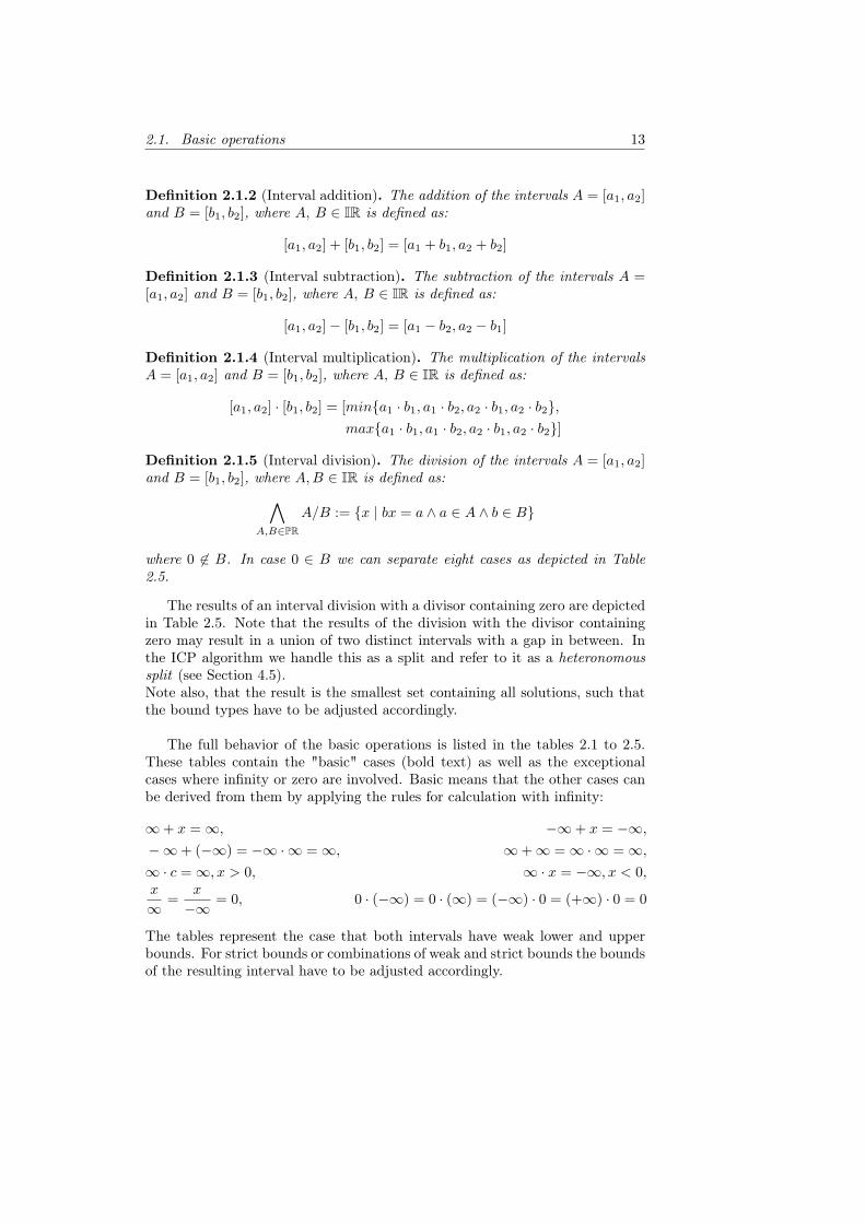
Definition 2.1.2 (Interval addition). The addition of the intervals A = [a1, a2]and B = [b1, b2], where A, B ∈ IR is defined as:

[a1, a2] + [b1, b2] = [a1 + b1, a2 + b2]

Definition 2.1.3 (Interval subtraction). The subtraction of the intervals A =[a1, a2] and B = [b1, b2], where A, B ∈ IR is defined as:

[a1, a2]− [b1, b2] = [a1 − b2, a2 − b1]

Definition 2.1.4 (Interval multiplication). The multiplication of the intervalsA = [a1, a2] and B = [b1, b2], where A, B ∈ IR is defined as:

[a1, a2] · [b1, b2] = [min{a1 · b1, a1 · b2, a2 · b1, a2 · b2},max{a1 · b1, a1 · b2, a2 · b1, a2 · b2}]

Definition 2.1.5 (Interval division). The division of the intervals A = [a1, a2]and B = [b1, b2], where A,B ∈ IR is defined as:∧

A,B∈PRA/B := {x | bx = a ∧ a ∈ A ∧ b ∈ B}

where 0 6∈ B. In case 0 ∈ B we can separate eight cases as depicted in Table2.5.

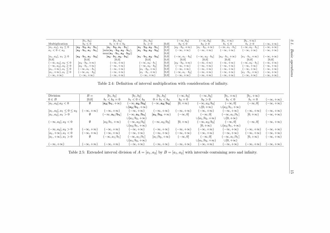
The results of an interval division with a divisor containing zero are depictedin Table 2.5. Note that the results of the division with the divisor containingzero may result in a union of two distinct intervals with a gap in between. Inthe ICP algorithm we handle this as a split and refer to it as a heteronomoussplit (see Section 4.5).Note also, that the result is the smallest set containing all solutions, such thatthe bound types have to be adjusted accordingly.

The full behavior of the basic operations is listed in the tables 2.1 to 2.5.These tables contain the "basic" cases (bold text) as well as the exceptionalcases where infinity or zero are involved. Basic means that the other cases canbe derived from them by applying the rules for calculation with infinity:

∞+ x =∞, −∞+ x = −∞,−∞+ (−∞) = −∞ ·∞ =∞, ∞+∞ =∞ ·∞ =∞,∞ · c =∞, x > 0, ∞ · x = −∞, x < 0,x

∞=

x

−∞= 0, 0 · (−∞) = 0 · (∞) = (−∞) · 0 = (+∞) · 0 = 0

The tables represent the case that both intervals have weak lower and upperbounds. For strict bounds or combinations of weak and strict bounds the boundsof the resulting interval have to be adjusted accordingly.


Addition (−∞, b2] [b1, b2] [b1,+∞) (−∞,+∞)(−∞, a2] (−∞, a2 + b2] (−∞, a2 + b2] (−∞,+∞) (−∞,+∞)[a1, a2] (−∞, a2 + b2] [a1 + b1,a2 + b2] [a1 + b1,+∞) (−∞,+∞)[a1,+∞) (−∞,+∞) [a1 + b1,+∞) [a1 + b1,+∞) (−∞,+∞)(−∞,+∞) (−∞,+∞) (−∞,+∞) (−∞,+∞) (−∞,+∞)

Table 2.1: Definition for interval addition with consideration of infinity.

Subtraction (−∞, b2] [b1, b2] [b1,+∞) (−∞,+∞)(−∞, a2] (−∞,+∞) (−∞, a2 − b1] (−∞, a2 − b1] (−∞,+∞)[a1, a2] [a1 − b2,+∞) [a1 − b2,a2 − b1] (−∞, a2 − b1] (−∞,+∞)[a1,+∞) [a1 − b2,+∞) [a1 − b2,+∞) (−∞,+∞) (−∞,+∞)(−∞,+∞) (−∞,+∞) (−∞,+∞) (−∞,+∞) (−∞,+∞)

Table 2.2: Definition for interval subtraction with consideration of infinity wherethe interval B = [b1, b2] is subtracted from the interval A = [a1, a2].

Division [b1, b2] [b1, b2] (−∞, b2] [b2,+∞)0 6∈ B b2 < 0 b1 > 0 b2 < 0 b1 > 0[a1, a2] , a2 ≤ 0 [a2/b1,a1/b2] [a1/b1,a2/b2] [0, a1/b2] [a1/b1, 0][a1, a2] , a1 ≤ 0 ≤ a2 [a2/b2,a1/b2] [a1/b1,a2/b1] [a2/b2, a1/b2] [a1/b1, a2/b1][a1, a2] , a1 ≥ 0 [a2/b2,a1/b1] [a1/b2,a2/b1] [a2/b2, 0] [0, a2/b1][0,0] [0,0] [0,0] [0,0] [0,0](−∞, a2], a2 ≤ 0 [a2/b1,+∞) (−∞, a2/b2] [0,+∞) (−∞, 0](−∞, a2], a2 ≥ 0 [a2/b2,+∞) (−∞, a2/b1] [a2/b2,+∞) (−∞, a2/b1][a1,+∞), a1 ≤ 0 (−∞, a1/b2] [a1/b1,+∞) (−∞, a1/b2] [a1/b1,+∞)[a1,+∞), a1 ≥ 0 (−∞, a1/b1] [a1/b2,+∞) (−∞, 0] [0,+∞)(−∞,+∞) (−∞,+∞) (−∞,+∞) (−∞,+∞) (−∞,+∞)

Table 2.3: Definition for interval division with consideration of infinity butwithout the divisor interval B containing zero.

2.1.Basic

operations15

[b1, b2] [b1, b2] [b1, b2] (−∞, b2] (−∞, b2] [b1,+∞) [b1,+∞)Multiplication b2 ≤ 0 b1 < 0 < b2 b1 ≥ 0 [0,0] b2 ≤ 0 b2 ≥ 0 b1 ≤ 0 b1 ≥ 0 (−∞,+∞)[a1, a2], a2 ≤ 0 [a2 · b2, a1 · b1] [a1 · b2, a1 · b1] [a1 · b2, a2 · b1] [0,0] [a2 · b2,+∞) [a1 · b2,+∞) (−∞, a1 · b1] (−∞, a2 · b1] (−∞,+∞)a1 < 0 < a2 [a2 · b1, a1 · b1] [min(a1 · b2, a2 · b1), [a1 · b2, a2 · b2] [0,0] (−∞,+∞) (−∞,+∞) (−∞,+∞) (−∞,+∞) (−∞,+∞)

max(a1 · b1, a2 · b2)] [0,0][a1, a2], a1 ≥ 0 [a2 · b1, a1 · b2] [a2 · b1, a2 · b2] [a1 · b1, a2 · b2] [0,0] (−∞, a1 · b2] (−∞, a2 · b2] [a2 · b1,+∞) [a1 · b1,+∞) (−∞,+∞)[0,0] [0,0] [0,0] [0,0] [0,0] [0,0] [0,0] [0,0] [0,0] [0,0](−∞, a2], a2 ≤ 0 [a2 · b2,+∞) (−∞,+∞) (−∞, a2 · b1] [0,0] [a2 · b2,+∞) (−∞,+∞) (−∞,+∞) (−∞, a2 · b1] (−∞,+∞)(−∞, a2], a2 ≥ 0 [a2 · b1,+∞) (−∞,+∞) (−∞, a2 · b2] [0,0] (−∞,+∞) (−∞,+∞) (−∞,+∞) (−∞,+∞) (−∞,+∞)[a1,+∞), a1 ≤ 0 (−∞, a1 · b1] (−∞,+∞) [a1 · b2,+∞) [0,0] (−∞,+∞) (−∞,+∞) (−∞,+∞) (−∞,+∞) (−∞,+∞)[a1,+∞), a1 ≥ 0 (−∞, a1 · b2] (−∞,+∞) [a1 · b1,+∞) [0,0] (−∞, a1 · b2] (−∞,+∞) (−∞,+∞) [a1 · b1,+∞) (−∞,+∞)(−∞,+∞) (−∞,+∞) (−∞,+∞) (−∞,+∞) [0,0] (−∞,+∞) (−∞,+∞) (−∞,+∞) (−∞,+∞) (−∞,+∞)

Table 2.4: Definition of interval multiplication with consideration of infinity.

Division B = [b1, b2] [b1, b2] [b1, b2] (−∞, b2] (−∞, b2] [b1,+∞) [b1,+∞)0 ∈ B [0,0] b1 < b2 = 0 b1 < 0 < b2 0 = b1 < b2 b2 = 0 b2 > 0 b1 < 0 b1 = 0 (−∞,+∞)[a1, a2].a2 < 0 ∅ [a2/b1,+∞) (−∞,a2/b2] (−∞,a2/b2] [0,+∞) (−∞, a2/b2] (−∞, 0] (−∞, 0] (−∞,+∞)

∪[a2/b1,+∞) ∪[0,+∞) ∪[a2/b1,+∞)[a1, a2], a1 ≤ 0 ≤ a2 (−∞,+∞) (−∞,+∞) (−∞,+∞) (−∞,+∞) (−∞,+∞) (−∞,+∞) (−∞,+∞) (−∞,+∞) (−∞,+∞)[a1, a2], a1 > 0 ∅ (−∞,a1/b1] (−∞,a1/b1] [a1/b2,+∞) (−∞, 0] (−∞, 0] (−∞, a1/b1] [0,+∞) (−∞,+∞)

∪[a1/b2,+∞) ∪[a1/b2,+∞) ∪[0,+∞)(−∞, a2], a2 < 0 ∅ [a2/b1,+∞) (−∞, a2/b2] (−∞, a2/b2] [0,+∞) (−∞, a2/b2] (−∞, 0] (−∞, 0] (−∞,+∞)

∪[a2/b1,+∞) [0,+∞) ∪[a2/b1,+∞)(−∞, a2], a2 > 0 (−∞,+∞) (−∞,+∞) (−∞,+∞) (−∞,+∞) (−∞,+∞) (−∞,+∞) (−∞,+∞) (−∞,+∞) (−∞,+∞)[a1,+∞), a1 < 0 (−∞,+∞) (−∞,+∞) (−∞,+∞) (−∞,+∞) (−∞,+∞) (−∞,+∞) (−∞,+∞) (−∞,+∞) (−∞,+∞)[a1,+∞), a1 > 0 ∅ (−∞, a1/b1] (−∞, a1/b1] [a1/b2,+∞) (−∞, 0] (−∞, 0] (−∞, a1/b1] [0,+∞) (−∞,+∞)

∪[a1/b2,+∞) ∪[a1/b2,+∞) ∪[0,+∞)(−∞,+∞) (−∞,+∞) (−∞,+∞) (−∞,+∞) (−∞,+∞) (−∞,+∞) (−∞,+∞) (−∞,+∞) (−∞,+∞) (−∞,+∞)

Table 2.5: Extended interval division of A = [a1, a2] by B = [a1, a2] with intervals containing zero and infinity.


Chapter 3

SMT solving

The goal of the presented ICP module is to speed up the search of an SMT solverfor a solution for quantifier-free nonlinear real arithmetic (QFNRA) formulae.SAT Modulo Theories (SMT) solving for the existential fragment of nonlinearreal algebra is able to cope with formulae of this type. At the beginning wepresent the theory fragment QFNRA and introduce definitions relevant for theremainder of this thesis. Afterwards we shortly sketch the general process ofSMT-solving. In the last section we introduce the underlying SMT toolboxSMT-RAT for the presented ICP module.

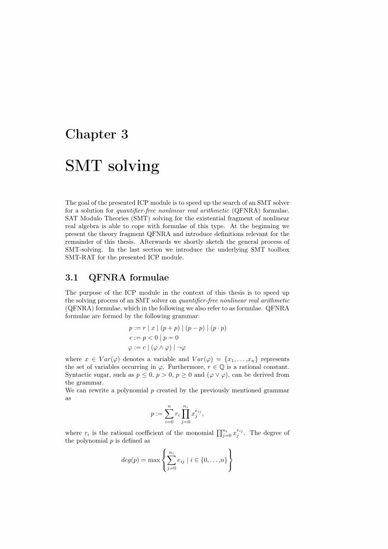
3.1 QFNRA formulaeThe purpose of the ICP module in the context of this thesis is to speed upthe solving process of an SMT solver on quantifier-free nonlinear real arithmetic(QFNRA) formulae, which in the following we also refer to as formulae. QFNRAformulae are formed by the following grammar:

p := r | x | (p+ p) | (p− p) | (p · p)c := p < 0 | p = 0

ϕ := c | (ϕ ∧ ϕ) | ¬ϕ

where x ∈ V ar(ϕ) denotes a variable and V ar(ϕ) = {x1, . . . ,xn} representsthe set of variables occurring in ϕ. Furthermore, r ∈ Q is a rational constant.Syntactic sugar, such as p ≤ 0, p > 0, p ≥ 0 and (ϕ ∨ ϕ), can be derived fromthe grammar.We can rewrite a polynomial p created by the previously mentioned grammaras

p :=

n∑i=0

ri

ni∏j=0

xeijj ,

where ri is the rational coefficient of the monomial∏ni

j=0 xeijj . The degree of

the polynomial p is defined as

deg(p) = max

ni∑j=0

eij | i ∈ {0, . . . ,n}

18 Chapter 3. SMT solving

The constraints can be separated into two groups: The set of linear constraints inϕ, Lϕ (deg(p) ≤ 1) and the set of nonlinear constraints in ϕ, Nϕ with deg(p) > 1,where p is the left-hand side of the constraint c. If Nϕ is empty we call ϕ aquantifier-free linear real arithmetic (QFLRA) formula.The set of variables which occur in nonlinear constraints of ϕ is denoted by VNϕ

while the set VLϕ denotes variables, which occur in linear constraints. Notethat the intersection VNϕ ∩ VLϕ does not have to be empty, as there might bevariables which occur in both linear and nonlinear constraints.The solving process for QFNRA formulae with current solvers is in the worstcase doubly exponential. Procedures to solve QFNRA formulae are cylindri-cal algebraic decomposition (CAD), virtual substitution (VS) or Gröbner basesamong others. The mentioned procedures have already been implemented asSMT-RAT modules. For QFLRA-solving there exist methods which are fast(polynomial) [Kha79]. The module implemented in SMT-RAT to solve QFLRAformulae is based on the Simplex algorithm [DM06, Dan98], which has an ex-ponential worst-case complexity. However, in practice it is the fastest approachby far.

3.2 Bounded NRA

The ICP method operates on bounded intervals, which requires that all vari-ables have to be bounded initially. In general it suffices to provide an over-approximating bound for every variable as long as this bound is given. This isrequired due to the behavior of the underlying interval arithmetic on unboundedintervals (see Section 2.1). Even if one bound for xj ∈ V ar(ϕ) is given whilethe other bound is not, interval arithmetic operations will most likely result incompletely unbounded intervals (−∞,+∞).Thus, we assume that each variable xj ∈ V ar(ϕ) has a corresponding interval[x]xj

∈ IR. Each interval has a lower and an upper bound such that we can sep-arate four cases, depending on the bound types (see Chapter 2):[x]xj

= [lj ,uj ],(lj ,uj), (lj ,uj ] or [lj ,uj) with lj , uj ∈ R, lj ≤ uj . We denote a point intervalas [c], c ∈ R, which stands for [c,c].We denote a vector of intervals [x] = ([x]x1

, . . . ,[x]xn)T ∈ IRn as a search box.

Definition 3.2.1. A search box of a given constraint set C is a vector of inter-vals [x] = ([x]x1 , . . . ,[x]xn) ∈ IRn for the variables occurring in C. Each intervalcan be represented independently by the conjunction of two linear constraints:

Φ([x]xj) =

lj ≤ xj ∧ xj ≤ uj iff [x]xj = [lj ,uj ]

lj < xj ∧ xj < uj iff [x]xj= (lj ,uj)

lj < xj ∧ xj ≤ uj iff [x]xj= (lj ,uj ]

lj ≤ xj ∧ xj < uj iff [x]xj= [lj ,uj)

and the search box can be represented by the conjunction of linear interval con-straints:

Φ([x]) =

n∧i=1

Φ([x]xi)

3.3. Classic SMT solving 19

Without loss of generality we can assume that constraints include only therelational symbols < , ≤ , =. A preprocessing in the ICP module enables us totransform all original constraints

ci :

n∑j=1

rj ·ni∏k=1

xejkk ∼ 0, ∼∈ {< , ≤ , =}

to the form

c′i : hi +

n∑j=1

rj ·ni∏k=1

xejkk = 0 (3.1)

such that all relations are encoded in the interval bound types of the additionalvariables hi. Therefore all constraints can be transformed to the required formof equations as demanded in Section 4.4.1.

Outlook Currently the ICP module demands a bounded initial search box. Itis still unresolved how to determine initial bounds efficiently. A rather inefficientway of obtaining initial bounds would be to pass all equations we gained afterthe preprocessing to a CAD implementation to project all polynomials occurringin the equations to univariate polynomials and then calculate Cauchy-bounds.The interval bounds would be the minimal and the maximal Cauchy-bound.

3.3 Classic SMT solving

ϕ

Boolean abstraction

SAT solver

(partial) assignment

Theory solver

infeasible subset

SAT/UNSAT

Figure 3.1: The classic SMT-solving approach.

As there are already very efficient SAT solvers, SMT-solving benefits froma combination of them, when combined with theory solving. At first a Booleanabstraction of the formula ϕ is created which is brought to conjunctive normal


form (CNF). The Boolean abstraction introduces a fresh Boolean variable forevery constraint in the original formula and keeps the Boolean skeleton intact.Converting the formula to CNF can be done efficiently by applying Tseitin’s en-coding [Tse68]. The SAT solver now tries to assign the variables of the Booleanabstraction in less-lazy DPLL style [GHN+04]. Each variable represents theabstraction of an original QFNRA subformula of the input formula. After eachassignment the set of asserted subformulae which are constraints is checked forconsistency by a theory solver. The difference to full-lazy SMT-solving is, thatin full-lazy SMT-solving the SAT-solver creates a full assignment for all Booleanvariables and afterwards hands the corresponding constraints over to the theorysolver.

The theory solver now tries to solve the given set of constraints. If the theorysolver finds a solution it informs the SAT solver about this and further decisionscan be made until a complete satisfying assignment is found. If the theory solvercannot find a solution because the set of constraints is unsatisfiable it providesinfeasible subsets of the checked set of constraints. Using this piece of informa-tion the conflict can be resolved and the search for a satisfying full assignmentof the Boolean variables whose corresponding set of constraints is consistent canbe continued. If no backtracking is possible as all available options have alreadybeen tried by the SAT solver the input formula is declared as unsatisfiable.Due to this behavior the underlying theory solver should support incrementalitywhich means that an belated assertion or a removal of a constraints results in aminimum of adjustments and already gained information which is not affectedcan be used for further computation. Furthermore, if the implementation sup-ports the creation of infeasible subsets and backtracking we refer to it as SMTcompliant.

3.4 SMT-RAT

The context in which the ICP module we present is used is the SMT-solvingtoolbox SMT-RAT [CLJA12]. The toolbox provides a set of modules, amongothers SMT compliant implementations of Gröbner bases, the virtual substi-tution and the cylindrical algebraic decomposition. Furthermore, SMT-RATmaintains a manager, which can use the provided modules to combine them toa solving strategy (see Figure 3.2).

Each module maintains received formulae Crec which is a set of QFNRAformulae the module is intended to solve. This set can be modified by usingthe provided functions assert(formula ϕ) and remove(formula ϕ). The centralmethod isConsistent() calls the consistency check of the actual received formu-lae Crec. As some of the contained modules are not complete (e.g. VS andGröbner bases) the modularity enables us to pass QFNRA formula sets to suc-ceeding modules in case they cannot be solved by the current module. This isreferred to as calling a backend and is performed by calling the function run-Backends(). When the consistency check fails it is intended to give a reason forthe failure, which is determined by sets of subsets of formulae Cinf called theinfeasible subset, where Cinf ⊆ 2Crec .

3.4. SMT-RAT 21

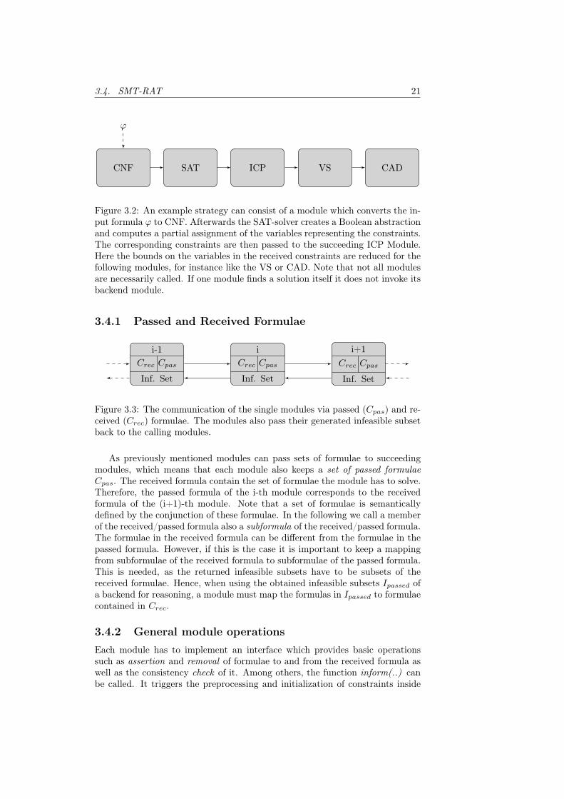
ϕ

CNF SAT ICP VS CAD

Figure 3.2: An example strategy can consist of a module which converts the in-put formula ϕ to CNF. Afterwards the SAT-solver creates a Boolean abstractionand computes a partial assignment of the variables representing the constraints.The corresponding constraints are then passed to the succeeding ICP Module.Here the bounds on the variables in the received constraints are reduced for thefollowing modules, for instance like the VS or CAD. Note that not all modulesare necessarily called. If one module finds a solution itself it does not invoke itsbackend module.

3.4.1 Passed and Received Formulae

i-1Crec Cpas

Inf. Set

iCrec Cpas

Inf. Set

i+1Crec Cpas

Inf. Set

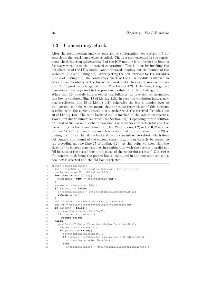
Figure 3.3: The communication of the single modules via passed (Cpas) and re-ceived (Crec) formulae. The modules also pass their generated infeasible subsetback to the calling modules.

As previously mentioned modules can pass sets of formulae to succeedingmodules, which means that each module also keeps a set of passed formulaeCpas. The received formula contain the set of formulae the module has to solve.Therefore, the passed formula of the i-th module corresponds to the receivedformula of the (i+1)-th module. Note that a set of formulae is semanticallydefined by the conjunction of these formulae. In the following we call a memberof the received/passed formula also a subformula of the received/passed formula.The formulae in the received formula can be different from the formulae in thepassed formula. However, if this is the case it is important to keep a mappingfrom subformulae of the received formula to subformulae of the passed formula.This is needed, as the returned infeasible subsets have to be subsets of thereceived formulae. Hence, when using the obtained infeasible subsets Ipassed ofa backend for reasoning, a module must map the formulas in Ipassed to formulaecontained in Crec.

3.4.2 General module operationsEach module has to implement an interface which provides basic operationssuch as assertion and removal of formulae to and from the received formula aswell as the consistency check of it. Among others, the function inform(..) canbe called. It triggers the preprocessing and initialization of constraints inside


a module. The management of infeasible subsets also happens according to amodule interface, called getInfeasibleSubsets().In the following paragraphs we sketch the purpose of the most important func-tions every module implements.

inform(constraint c)

The purpose of the method inform(constraint c) is to be able to perform allpossible preprocessing before the assertion of formulae. This requires that amodule is informed about all possible constraints before adding formulae withassert(formula ϕ) which contain them.

assert(formula ϕ)

The general difference between assert(..) and inform(..) can be described asfollows: While inform(..) just determines the set of constraints a module willpossibly encounter, assert(formula ϕ) indicates that a formula ϕ has been addedto the received formula. During assert(formula ϕ) all operations should beperformed which are needed to activate constraints of ϕ for a later consistencycheck.

remove(formula ϕ)

The method remove(formula ϕ) is called in order to indicate, that ϕ is removedfrom the received formulae Crec. With the removal of a formula all resultsgained from calculations including this formula need to be removed as well.The remaining results from calculations of formulae ψ ∈ Crec, ψ 6= ϕ shouldstay untouched.

isConsistent()

The method isConsistent() is called to check the consistency of current receivedformulae. Note that a call to runBackends() conforms to calling the methodisConsistent() of the succeeding module. The function performs the solvingand returns an answer of the type "True", "False" or "Unknown". In case theanswer is "False", the module should be able to provide an explanation in theform of an infeasible subset.

getInfeasibleSubsets()

The method getInfeasibleSubsets() is called in order to return the infeasiblesubsets to the preceding module in case the consistency check evaluated toFalse.

Chapter 4

The ICP module

In this section we provide background information about the Interval ConstraintPropagation (ICP) module which is inspired by the approach by Gao et al.[GGI+10]. The module can be separated in the four major parts preprocessing,contraction, splitting and validation. First, we present the general module inthe first section. The next sections cover further details of the module, startingwith the preprocessing of the given constraints. The central element of thealgorithm, the contraction of intervals, is described afterwards. This sectionalso contains information about the proper selection of contraction candidates.When the algorithm has come to a fixpoint, an autonomous split can advance theprocedure and provide new possibilities of progress. After a solution candidatehas been found this candidate has to be verified during the validation part ofthe algorithm.

4.1 Algorithm

In this section we present the basic functionality of the ICP module. Note thatthe input formula of a general module is a set of subformulae, which is definedas the conjunction of the subformulae. The ICP module can only perform aconsistency check on a set of constraints and returns "Unknown" if this is notthe case. The Sections 4.2 to 4.6 deal with this consistency check, whereas Sec-tion 4.7 explains how incremental manipulation of the received formula of theICP module is performed.

As the module is designed to be part of a whole solver strategy as well asto be usable standalone, a preprocessing has to be included. This ensures, thatall constraints are put in the correct format for further processing, no matterin which way the module is used. The main idea of the preprocessing is to splitnonlinear constraints from the linear ones and to transform all constraints toequations. The former is achieved by introducing a fresh real-valued variablevm for each nonlinear monomial m, replace all occurrences of m in the consid-ered constraint by vm and add the equation vm = m. The latter is done byintroducing fresh variables to obtain equations (see Section 4.2).After the preprocessing the actual contraction of the intervals takes place. Thealgorithm chooses the next possible combination of constraint and variable, we

24 Chapter 4. The ICP module

refer to as the contraction candidate (see Definition 4.4.1), by a certain heuris-tic (see Section 4.4.2), in order to apply contraction. The algorithm repeatschoosing a contraction candidate and contracting until we fulfill the precisionrequirements (see Section 4.6.2), i.e. a given target diameter for all intervals ofthe current search box is reached, or there is no contraction candidate contract-ing the search box sufficiently, what we refer to as fixpoint.If the latter case occurs, the search box is split in half and contraction is re-sumed on the gained search box (see Section 4.5). After reaching a point wherethe precision requirements are met, the contraction is stopped and the resultingsearch box is handed over to the validation. After successfully validating thebox against the linear feasible region it possibly contains a solution. We verifythe existence of a solution in this box by an according backend call. In caseof an unsuccessful validation either the violated linear constraints are added ascontraction candidates or if already existing the box is set as (unsuccessfully)validated (see Section 4.6). If contraction leads to an empty set the box is dis-carded as a possible solution and the algorithm continues with the next possiblebox (see Section 4.5.1).

4.2 PreprocessingLinear and nonlinear constraints are separated during the preprocessing (line 3)and ICP mainly performs on the nonlinear constraints, because firstly there arealready efficient algorithms to solve linear constraints [DM06] and secondly ICPis known to suffer from the slow convergence problem, which can occur, whenwe perform ICP on linear constraints (see Example 4.4.2).Therefore it is important to detect the nonlinear parts in the given constraintset, such that ICP initially can be applied on nonlinear constraints only. Thepreprocessing we implement in the ICP module is related to the approach pre-sented by Gao et al. [GGI+10].For every new nonlinear mononomial mi of the left-hand side of the consideredconstraint ci (see Section 3.1) we introduce a fresh nonlinear variable ni suchthat we obtain a new constraint mi − ni = 0. Additionally to keep the originalstructure, the nonlinear part in the original constraint ci is replaced by the newlyintroduced variable ni. To be able to cope with relational symbols in the nowlinearized constraints, we add a new slack variable si for every new (linearized)left-hand side, set the relation to equality and add the bound correspondingly.Assume, we have the nonlinear constraint

n∑i=0

ci

ni∏j=0

xeijj ∼ b,∼∈ {< , ≤},

we replace∏ni

j=0 xeijj by a fresh real-valued variable mi. For all linear con-

straints∑cimi we equalize it by adding a slack variable si gaining the equation

−si +∑cimi and add the bound si ∼ b. Note that we introduce only one

nonlinear variable for equal nonlinear monomials and only one slack variable forequal linear left-hand sides without constant parts.This is done because the ICP algorithm demands equations as input, which aregained by using the bounds of the slack variables to represent possible inequa-tions.

4.2. Preprocessing 25

Example 4.2.1 (Preprocessing). Original constraints given to the module:

[x2 − 1− y = 0 ∧ x− y ≤ 0]

Add nonlinear variable n1 for x2: First add the identity x2−n1 = 0 and replaceall occurrences of x2 in the original constraints to obtain linearized constraints:

[x2 − n1 = 0 ∧ n1 − 1− y = 0 ∧ x− y ≤ 0]

Introduce slack variables for the linear constraints:

[x2 − n1 = 0 ∧ n1 − 1− y = 0 ∧ x− y − s1 = 0 ∧ s1 ≤ 0]

It is important to keep the mapping from the original constraints to thepreprocessed ones as for the communication to the other modules we need toremember the original constraints. If we, for instance, obtain an infeasible subsetfrom a backend and we want to use it for the construction of the ICP module’sinfeasible subset, it is necessary to look up the correct preprocessed originalconstraints. We introduce a mapping from original constraints to linearizedones and from linearized constraints to the corresponding equations with slackvariables to achieve this (see Section 4.7).

After the preprocessing, the obtained linear equations are passed to an in-ternal LRA module implemented according to [DM06] – the method inform(..)of the LRA module is called with the linearized constraint (line 4). Due to thefact that the internal LRA module is implemented as an SMT-RAT module itis accessed by the same functions inform(..), assert(..), remove(..) and isCon-sistent().

At this point we already have all information required for the creation of thenonlinear contraction candidates (line 5). Note that we use the LRA module’sinternal slack variables, which are created in the aforementioned fashion. Thelinear contraction candidates are held in a mapping, which maps the slack vari-ables of the LRA module to the linear contraction candidates. Furthermore, weinform the backend about the new constraints.

1 inform(Constraint _constr)2 {3 (linearConstraint, [nonlinearReplacements]) = linearize(_constr);4 informLRASolver(linearConstraint);5 createNonlinearCandidates([nonlinearReplacements]);6 informBackend(_constr);7 }

Listing 4.1: The method inform(constraint), which is called at first to performpreprocessing.

Outlook Currently, we use the constraints from the received formula of theICP module as the constraints for the backends. It is also possible to pass thepreprocessed constraints to the backend which saves transformation time in casewe need the infeasible subset returned by the backend for internal purposes anddo not intend to pass the gained infeasible subset to a preceding module.


4.3 Consistency checkAfter the preprocessing and the assertion of subformulae (see Section 4.7 forassertion), the consistency check is called. The first step executed in the consis-tency check function isConsistent() of the ICP module is to obtain the boundsfor every variable in the linearized constraints. This is done by invoking theinitialization of the LRA module and afterwards reading out the bounds of thevariables (line 3 of Listing 4.2). After getting the new intervals for the variables(line 5 of Listing 4.2), the consistency check of the LRA module is invoked tocheck linear feasibility of the linearized constraints. In case of success the ac-tual ICP algorithm is triggered (line 12 of Listing 4.2). Otherwise, the gainedinfeasible subset is passed to the previous module (line 10 of Listing 4.2).When the ICP module finds a search box fulfilling the precision requirements,this box is validated (line 13 of Listing 4.2). In case the validation fails, a newbox is selected (line 15 of Listing 4.2), otherwise the box is handed over tothe backend module, which means that the consistency check of this backendis called with the current search box together with the received formula (line20 of Listing 4.2). The same backend call is invoked, if the validation rejects asearch box due to numerical errors (see Section 4.6). Depending on the solutionreturned of the backend, either a new box is selected for contraction (in case thebackend rejects the passed search box, line 24 of Listing 4.2) or the ICP modulereturns "True" (in case the search box is accepted by the backend, line 29 ofListing 4.2). Note that if the backend returns an infeasible subset, which doesnot contain any bound of the current search box, it can directly be passed tothe preceding module (line 27 of Listing 4.2). At this point we know that thecheck of the current constraint set in combination with the current box did notfail because of the passed box but because of the constraint set itself. Otherwiseif a constraint defining the passed box is contained in the infeasible subset, anew box is selected and the old box is rejected.

1 Answer isConsistent(){2 initializeLRA(); // creates intervals for variables3 variables = getVariablesFromLRA();4 for (var in variables){5 currentBox[var] = getIntervals(var);6 }7 answer = isConsistentLRA();8 if (answer == false){9 infeasibleSubset = getInfeasibleSubsetFromLRA();10 return answer;11 }12 solutionCandidateBox = contract(currentBox)13 answer = validateSolution(solutionCandidateBox);14 if (answer = false){15 currentBox = selectNextBox();16 if (currentBox == NULL)17 return false;18 }else{19 pushBoundsToPassedFormula(solutionCandidateBox);20 answer = callBackends();21 if (answer = false){22 createInfeasibleSubset();23 if (infeasibleSubsetContains(solutionCandidateBox))24 currentBox = selectNextBox();25 else26 infeasibleSubset = getInfeasibleSubsetFromBackend();

4.4. Contraction/ICP 27

27 return false;28 }else{29 return answer;30 }31 }32 }

Listing 4.2: The procedure isConsistent calls the ICP algorithm and managesalso the validation as well as the calling of backends.

The detailed methods used during the consistency check are described during thefollowing sections starting with the contraction of intervals which is performedby the ICP algorithm giving this module its name.

4.4 Contraction/ICPIn our version of the ICP algorithm, the contraction of intervals is performed byan interval extension of Newton’s method [Moo77, HR97]. In general each con-traction takes a constraint as well as a variable occurring in the constraint anduses this to contract the interval of the variable. We refer to this combinationas a contraction candidate:

Definition 4.4.1. A contraction candidate c is a tuple

c = 〈fi, xj〉, fi = 0 ∈ Nϕ ∪ Lϕ, xj ∈ V ar(fi) (4.1)

where V ar(fi) denotes the set of variables contained in fi. Note that the con-straint fi = 0 is taken from the set of preprocessed constraints Nϕ ∪ Lϕ whichare generated from the input formula ϕ.

Each contraction candidate holds a weight which measures the importanceof this candidate during the past contractions and is updated after each con-traction according to a weighting function (see Section 4.4.2). Having chosen acontraction candidate, the actual contraction of the interval of the correspondingvariable can be started.

1 contract(IntervalBox _box){2 relevantCandidates = updateRelevantCandidates();3 while ( !relevantCandidatesEmpty() && !targetSizeReached){4 candidate = chooseCandidate(relevantCandidates);5 splitOccured = Newton(candidate, _box);6 if(!splitOccured)7 {8 addContractionToHistoryNode(candidate);9 addAllAffectedCandidatesToRelevant();

10 }11 else12 {13 performSplit(candidate);14 }15 updateWeight(candidate);16 relevantCandidates = updateRelevantCandidates();17 }18 }

Listing 4.3: Contraction in pseudo-code. The function updateRelevantCandi-dates keeps the sorted mapping of relevant candidates up to date (see Paragraph4.4.2 for details).


4.4.1 Newton’s method

−2 −1 1 2 3

−1

1

2

3

4

x1x2

x2 = x1 − f(x1)f ′(x1)

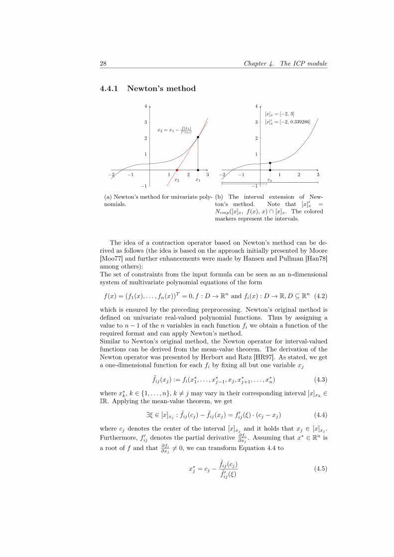
(a) Newton’s method for univariate poly-nomials.

−2 −1 1 2 3

−1

1

2

3

4

cx

[x]x = [−2, 3]

[x]′x = [−2, 0.339286]

(b) The interval extension of New-ton’s method. Note that [x]′x =Ncmp([x]x, f(x), x) ∩ [x]x. The coloredmarkers represent the intervals.

The idea of a contraction operator based on Newton’s method can be de-rived as follows (the idea is based on the approach initially presented by Moore[Moo77] and further enhancements were made by Hansen and Pullman [Han78]among others):The set of constraints from the input formula can be seen as an n-dimensionalsystem of multivariate polynomial equations of the form

f(x) = (f1(x), . . . , fn(x))T = 0, f : D → Rn and fi(x) : D → R, D ⊆ Rn (4.2)

which is ensured by the preceding preprocessing. Newton’s original method isdefined on univariate real-valued polynomial functions. Thus by assigning avalue to n− 1 of the n variables in each function fi we obtain a function of therequired format and can apply Newton’s method.Similar to Newton’s original method, the Newton operator for interval-valuedfunctions can be derived from the mean-value theorem. The derivation of theNewton operator was presented by Herbort and Ratz [HR97]. As stated, we geta one-dimensional function for each fi by fixing all but one variable xj

f̃ij(xj) := fi(x∗1, . . . , x

∗j−1, xj , x

∗j+1, . . . , x

∗n) (4.3)

where x∗k, k ∈ {1, . . . , n}, k 6= j may vary in their corresponding interval [x]xk∈

IR. Applying the mean-value theorem, we get

∃ξ ∈ [x]xj: f̃ij(cj)− f̃ij(xj) = f ′ij(ξ) · (cj − xj) (4.4)

where cj denotes the center of the interval [x]xjand it holds that xj ∈ [x]xj

.Furthermore, f ′ij denotes the partial derivative ∂fi

∂xj. Assuming that x∗ ∈ Rn is

a root of f and that ∂fi∂xj6= 0, we can transform Equation 4.4 to

x∗j = cj −f̃ij(cj)

f̃ ′ij(ξ)(4.5)


because x∗ is a root of fi as well. If we replace the indeterminate ξ by the wholeinterval [x]xj

we end at

N := cj −f̃ij(cj)

f̃ ′ij([x]xj), (4.6)

x∗j ∈ N

As stated above, the partial derivative should not be equal to zero. However, inthis setting it can happen that the resulting interval of the derivative containszero. In this case we make use of extended interval division (see Table 2.5)which results in an interval with a gap (a heteronomous split, see Section 4.5).Nevertheless, we do not have any information of the remaining zeroes containedin x∗ – the only information we have is that they are contained in their intervals[x]xj , j ∈ {1, . . . ,n} which defines the search box [x] = ([x]x1 , . . . , [x]xn)T ∈ IRn.If we replace each x∗i , i ∈ {1, . . . ,n} by its corresponding interval, due to inclu-sion monotonicity we obtain a superset of N :

N ⊆ cj −fi([x]x1 , . . . , [x]xj−1 , cj , [x]xj+1 , . . . , [x]xn)

∂fi∂xj

([x]x1 , . . . , [x]xn)(4.7)

Note that the subtraction of an interval from a number (here: cj) can be handledby treating cj as a point interval such that cj − [a, b] = [cj , cj ] − [a, b] = [cj −b, cj − a].We are now able to define the interval Newton operator, which uses the i-thequation of the equation system to treat the j-th component of the search box :

Definition 4.4.2. Let D ⊆ Rn, f : D → Rn, f = (f1, . . . ,fn)T be a con-tinuously differentiable function, and let [x] = ([x]x1

, . . . ,[x]xn)T ∈ IRn be an

interval vector with [x] ⊆ D and i, j ∈ {1, . . . ,n}. Then the component-wiseinterval Newton operator Ncmp is defined by:

Ncmp([x], i, j) := cj −fi([x]x1 , . . . , [x]xj−1 , cj , [x]xj+1 , . . . , [x]xn)

∂fi∂xj

([x]x1 , . . . , [x]xn)(4.8)

The arguments of the component-wise interval Newton operator are the rea-son for the structure of the contraction candidates which contain the neededparameters i and j (see Definition 4.4.1). Herbort and Ratz elaborated twoimportant properties concerning the existence of a zero of the component-wiseinterval Newton operator Ncmp [HR97]:

Theorem 4.4.1. Let D ⊂ Rn, f : D → Rn be a continuously differentiablefunction, and let [x] = ([x]x1

, . . . ,[x]xn)T ∈ IRn be an interval vector with [x] ⊆

D. Then the component-wise interval Newton operator Ncmp has the followingproperties:

1. Let x∗ ∈ [x] be a zero of f , then we have for arbitrary i, j ∈ {1, . . . ,n} :x∗ ∈ ([x]x1

, . . . , [x]xj−1,Ncmp([x], i, j), [x]xj+1

, . . . , [x]xn)

2. If Ncmp([x], i, j) ∩ [x]xj= ∅ for any i, j ∈ {1, . . . ,n} then there exists no

zero of f in [x].


Proof. Herbort and Ratz prove their first statement by referring to the deriva-tion of the Ncmp operator. Let x∗ ∈ [x] be a zero of f , and let i, j ∈ {1, . . . ,n}.If we take fi as a one-dimensional real-valued function in xj , we can derive fromthe mean-value theorem (see Equation 4.4):

x∗j = cj −fi(x

∗1, . . . , x

∗j−1, cj , x

∗j+1, . . . , x

∗n)

∂fi∂xj

(x∗1, . . . , x∗j−1, ξ, x

∗j+1, . . . , x

∗n), ξ ∈ [x]xj

(4.9)

with cj := m([x]xj) and assuming that ∂fi

∂xj(. . .) 6= 0. As we know that x∗ ∈ [x]

and especially x∗j ∈ [x]xj we do not lose validity if we replace the unknown ξby the whole interval [x]xj

– in fact we include x∗j . If we additionally replaceevery x∗k, k 6= j by its corresponding interval [x]xk

(as we do not know the exactcomponent x∗k but the same statement x∗k ∈ [x]xk

holds) we get a superset ofthe previous inclusion:

x∗j ∈ cj −fi(x

∗1, . . . , x

∗j−1, cj , x

∗j+1, . . . , x

∗n)

∂fi∂xj

(x∗1, . . . , x∗j−1, [x]xj

, x∗j+1, . . . , x∗n)

(inclusion) (4.10)

⊆ cj −fi([x]x1 , . . . , [x]xj−1 , cj , [x]xj+1 , . . . , [x]xn)

∂fi∂xj

([x]x1 , . . . , [x]xj−1 , [x]xj , [x]xj+1 , . . . , [x]xn)(4.11)

= Ncmp([x], i, j) . (4.12)

As only the j-th component of [x] is treated we can conclude that

x∗ ∈ ([x]x1 , . . . , [x]xj−1 , Ncmp([x], i, j), [x]xj+1 , . . . , [x]xn) . (4.13)

By using the first statement of the theorem the second one can be proven usingcontradiction. We assume that there exists a zero x∗ ∈ [x] of f and we assumethat Ncmp([x], i, j) ∩ [x]xj

= ∅. If we apply the Newton operator with somearbitrary i, j ∈ {1, . . . , n} we get:

x∗j ∈ Ncmp([x], i, j) ⊆ Ncmp([x], i, j) ∩ [x]xj= ∅ . (4.14)

This neglects the assumed zero and proves the second statement by contradic-tion.

Both statements from Theorem 4.4.1 have an important meaning for the ap-plication of the component-wise interval Newton operator in the ICP algorithmfor contraction. The first statement ensures that regardless of how often aninterval is contracted by a contraction candidate, we do not lose a solution – allzeros in the initial search box are always contained in the resulting search box.The second statement is useful in rejecting possible search boxes: If the con-secutive application of the component-wise interval Newton operator on a givensystem of equations results in an empty set, the original search box did not con-tain any zeros. This has two important implications for the data structure ofthe ICP module: Firstly, if we are able to contract a box to the empty intervalwe can drop the whole box and, secondly, it suffices to store the contractionswhich are applied on a certain box instead of storing each resulting box afterone contraction step. This is because if we are able to create the empty set viacontraction we can drop all previously made contractions until the point where


the box has been created, e.g. by a split (see Section 4.5.1 for details of thedata structure).

After contraction, the result is intersected with the original interval of thevariable before contraction. Therefore, the resulting interval is at least as wide asthe original one. This is done to prevent the method from diverging. Due to thisapproach, if the actual setup tends to diverge, the resulting relative contractionequals zero and thus, the contraction candidate is rated down. The rating ofcontraction candidates is done via the relative contraction and the weight isupdated after each successful contraction (see Section 4.4.2). Successful in thiscase means that the relative contraction is above a predefined threshold and thecontraction did not result in an empty interval.

Example 4.4.1 (Contraction). We choose the constraint set from previous ex-amples but omit the preprocessing to increase readability: C = [c1 : x2 − y =0 ∧ c2 : x− y = 0]. The initial search box is set as: [x] ∈ IR2 = [1, 3]x × [1, 2]y.If we consider the two contraction candidates 〈c1, x〉 and 〈c2, y〉 and alter theirapplication, we gain a contraction sequence. We show the first contraction indetail with the previously mentioned Newton operator:

Ncmp([1, 3]x × [1, 2]y, x2 − y = 0, [1, 3]x) = [2, 2]− [2, 2]2 − [1, 2]

2 · [1, 3]

= [2, 2]− [2, 3]

[2, 6]

= [0.5, 1.66667]

what results in an updated interval for x : [1, 3]c1,x→ [1, 3] ∩ [0.5, 1.66667] =

[1, 1.66667]. If we now alter the contraction candidates we obtain the sequence:

[1, 3]xc1,x→ [1, 1.66667]x

c1,x→ [1, 1.3]xc1,x→ [1, 1.14135]x

c1,x→ . . .c1,x→ [1, 1]x

[1, 2]yc2,y→ [1, 1.66667]y

c2,y→ [1, 1.3]yc2,y→ [1, 1.14135]y

c2,y→ . . .c2,y→ [1, 1]y

As mentioned in Section 4.2, the presented preprocessing approach separatesnonlinear and linear constraints. This is done due to the fact that ICP isvulnerable to slow convergence. We can outline this behavior by an example:

Example 4.4.2 (Slow convergence). Consider the constraint set C = [c1 :y = x + 1 ∧ c2 : x = y + 1]. If we limit the initial box, e.g.: [x] ∈ IR2 =[1, n]x × [1, n]y, n ∈ N, we observe, that the constraint system is unsatisfiable.However the contraction sequence of the ICP algorithm would look like

[1, n]xc2,x→ [2, n]x

c2,x→ [3, n]xc2,x→ [4, n]x

c2,x→ . . .

[1, n]yc1,y→ [2, n]y

c1,y→ [3, n]yc1,y→ [4, n]y

c1,y→ . . .

until the system is finally declared unsatisfiable. A linear solver would find thisfact without taking 2n contraction steps.

Outlook The contraction as described above is the first approach to con-tract intervals. Herbort and Ratz [HR97] mention extensions to the presentedcomponent-wise Newton operator: The usage of index lists is one of them.


The introduction of index lists aims at improving the choice of the best possiblecontraction candidate. The idea is to use automatic differentiation to determineall partial derivatives, which corresponds to a single evaluation of the Jacobianmatrix of the system. This is done because if the derivative equals zero (thedenominator in Equation 4.8) and the numerator contains zero the result willbe (−∞,+∞), which does not contribute to the solution and, thus, can directlybe avoided.According to [HR97] it is sufficient to choose only candidates from the obtainedJacobian matrix with entries different from zero. This results in a set of possiblecontraction candidates. However, the order of those candidates is still to be de-termined. The idea is to successively use all possible variables on one constraintas this results in an interval at least as small as if we choose the optimal variabledirectly. In fact it can be even smaller – the next optimal step can be in the setof remaining candidates

Remark 4.4.1 (Index Lists). Let S := (〈ci, x1〉, . . . , 〈ci, xn〉), j ∈ {1, . . . , n}, n :=|V ar(ci)| be the unknown optimal contraction sequence for the constraint ciwhere each variable xk, k ∈ {1, . . . , n} occurs exactly once. It can be assuredthat the resulting relative contraction c when using a sequence S ′ 6= S is at leastas big as if the first contraction candidate of S is chosen directly.

Herbort and Ratz propose the usage of two index lists L1 and L2. The firstone contains all pairs (i, j), where the entry in the calculated Jacobian is dif-ferent from zero while the second list contains all pairs where extended intervaldivision has to be applied.The items for L1 are picked starting from the diagonal element of the calculatedJacobian matrix and proceeding downwards and jumping to the first row if thebottom is reached.The list L2 is created by choosing the element with the largest diameter fromeach column whose entry is equal to zero.

4.4.2 Choice of the Contraction CandidateDuring the contraction of the given search box we can choose between severalcontraction candidates, as we usually have more than one asserted constraintwith more than one variable. However, not all candidates will result in the samerelative contraction. Even worse, the possible relative contraction is dependenton the order and appearance of the previous contractions.This means that, on the one hand, we cannot predict the possible relative con-traction of a contraction candidate and, on the other hand, the possible relativecontraction changes during time. Goualard and Jermann [GJ08] have relatedthis problem to a standard problem in reinforced learning, the multi-armed ban-dit problem. This problem is described as follows.There are k slot machines with an unknown probability to win and a fixed timehorizon. The goal is to find a sequence of levers to pull such that the out-come is maximized in the given time horizon. In our case the slot machines arethe contraction candidates and the outcome is the relative contraction. Thereexists a non-stationary version of the problem where the probabilities of theslot machines to win change non-deterministically while time passes. The non-stationary version of this problem is closely related to our problem as the re-


sulting contraction is not predictable until the actual calculation is done andvaries during time.

If we consider our equation system of n equations with at most n vari-ables, we have to choose between n2 contraction candidates before every singlecontraction. As previously mentioned, there is no way to predict the relativecontraction of a candidate such that we stick to heuristics. Goualard and Jer-mann [GJ08] propose a reinforced learning approach for this problem which weadapt.The basic idea of this learning approach is to rate every applied contraction suchthat the weight W (ij) of every contraction candidate represents its importanceduring the past solving process. Goualard proposes an update formula whoseresult represents the average of the last contractions biased with a factor αwhich introduces a parameter to adjust the effect of the last applied contractionon the whole weight

W(ij)k+1 = W

(ij)k + α(r

(ij)k+1 −W

(ij)k ) (4.15)

where r(ij)k+1 represents the last contraction and W (ij)k the previous weight of the

candidate. The factor α has a strong influence on how the weights evolve: Is αclose to 0, for example α = 0.1, the initial weight has a longterm influence onthe weights. On the other hand, if we pick a value close to 1, e.g. α = 0.9, theweights change with faster pace and the last payoffs have a stronger impact onthe weighting. In our approach we choose a value of α = 0.9, as the importanceof certain candidates in our examples varied a lot. Nevertheless, this factor isone of the many relevant parameters which can be tuned to change the behaviorof the whole algorithm. Therefore, the optimal setting of this parameter stillhas to be determined.After picking a contraction candidate, the actual contraction is performed withthe component-wise interval Newton operator Ncmp (see Section 4.4.1). Afterthe contraction, the relative contraction is computed and the weight of the cho-sen contraction candidate is updated.

ICP-relevant candidates Currently we keep a sorted mapping of weightsto contraction candidates, which we refer to as "ICP-relevant candidates". Inthis mapping it is easy to pick the candidate with the highest weight, as it islocated at the last position in the mapping. Due to the improbable but stillpossible case, that two candidates have the same weight, we extended the keyof the ICP-relevant candidates to a tuple (weight, id), where the id is set uponcreation of the contraction candidate by an internal manager.If a relative contraction above a certain threshold has been made, the candidateis kept in the mapping, otherwise it is removed. Additionally, all candidateswhich contain the variable whose interval has changed and are active (see Section4.6), are added to the ICP-relevant candidates.This ensures that all candidates which could profit from a changed interval areenlisted and are at least considered once for contraction. This implies, that eachchange is eventually propagated throughout the whole system, as every affectedcontraction candidate, which is active is added as a relevant candidate.


Outlook As previously mentioned, the influence of the parameter α may be ofinterest during the proper selection of the next contraction candidate. Further-more, Herbort and Ratz introduced index lists which also might be of interest toimprove the algorithm [HR97]. In their paper Goualard and Jermann proposeto use priority queues for every variable which should ensure that each variableis eventually used for contraction [GJ08]. The current approach via the weightsallows, that a limited number of contraction candidates are chosen alternately,which might suppress the reduction of all variables. However, the current imple-mentation also stops reducing one variable if the target diameter of its intervalhas been reached such that this suppression is only temporary.Another small optimization is to use linear contraction candidates only once asthe relative contraction of a linear candidate equals zero if it is applied morethan once consecutively.

4.5 Split

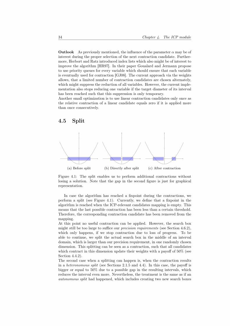
(a) Before split (b) Directly after split (c) After contraction

Figure 4.1: The split enables us to perform additional contractions withoutlosing a solution. Note that the gap in the second figure is just for graphicalrepresentation.

In case the algorithm has reached a fixpoint during the contractions, weperform a split (see Figure 4.1). Currently, we define that a fixpoint in thealgorithm is reached when the ICP-relevant candidates mapping is empty. Thismeans that the last possible contraction has been less than a certain threshold.Therefore, the corresponding contraction candidate has been removed from themapping.At this point no useful contraction can be applied. However, the search boxmight still be too large to suffice our precision requirements (see Section 4.6.2),which only happens, if we stop contraction due to loss of progress. To beable to continue, we split the actual search box in the middle of an intervaldomain, which is larger than our precision requirement, in one randomly chosendimension. This splitting can be seen as a contraction, such that all candidateswhich contract in this dimension update their weights with a payoff of 50% (seeSection 4.4.2).The second case when a splitting can happen is, when the contraction resultsin a heteronomous split (see Sections 2.1.5 and 4.4). In this case, the payoff isbigger or equal to 50% due to a possible gap in the resulting intervals, whichreduces the interval even more. Nevertheless, the treatment is the same as if anautonomous split had happened, which includes creating two new search boxes

4.5. Split 35

and enlisting them into the history tree.

4.5.1 History Tree

Root, id: 1

Contractions: [∅]

Split:

[x]init

id: 2Contractions: [. . .]

Split: x1


Split: x2

id: 4Contractions: ∅

Split:


Split: x4

id: 6Contractions: ∅

Split:

...

id: iContractions: ∅

Split:

id: i+1Contractions: ∅

Split:

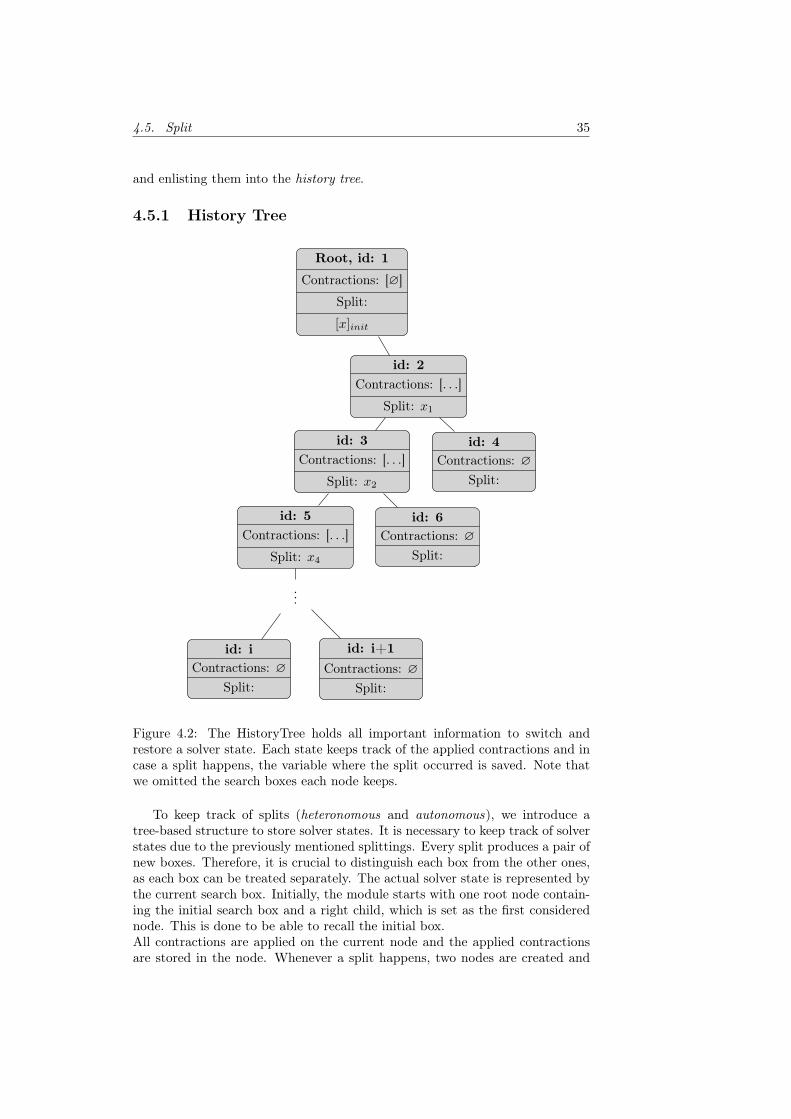
Figure 4.2: The HistoryTree holds all important information to switch andrestore a solver state. Each state keeps track of the applied contractions and incase a split happens, the variable where the split occurred is saved. Note thatwe omitted the search boxes each node keeps.

To keep track of splits (heteronomous and autonomous), we introduce atree-based structure to store solver states. It is necessary to keep track of solverstates due to the previously mentioned splittings. Every split produces a pair ofnew boxes. Therefore, it is crucial to distinguish each box from the other ones,as each box can be treated separately. The actual solver state is represented bythe current search box. Initially, the module starts with one root node contain-ing the initial search box and a right child, which is set as the first considerednode. This is done to be able to recall the initial box.All contractions are applied on the current node and the applied contractionsare stored in the node. Whenever a split happens, two nodes are created and


appended to the current node. Each new node contains one half or less of theoriginal search box. Additionally, the old node sets a variable indicating inwhich dimension it has been split.To be able to get infeasible subsets, all nodes keep track of their applied contrac-tions, such that we can apply a simple backtracking mechanism if needed. Thisincludes that a set of references to the used contraction candidates is stored,where each candidate occurs at most once.When selecting a new state in the tree, the current considered intervals con-cerned for contraction are set to this state (see also lines 15 and 24 in Algorithm4.2). The selection of the next state follows a left-most depth-first traversal ofthe tree. When selecting a new box, the older nodes left of the new node can bedeleted. This keeps the tree in an almost linear structure, as every split resultsin two nodes from which only one is considered. Furthermore, the old nodes arenot of interest any more as they were already visited.

1

2 3

4 5

...

i i+1

Figure 4.3: The choice of the next solver state is done in a left-most depth-firstmanner. Note that when switching the solver state all visited nodes are cut tokeep the overall number of nodes small.

Outlook Currently, the splitting creates an almost linear binary tree. Au-tonomous splits divide an interval into two equal parts by cutting in the middleof the interval of the desired dimension.One variation of this approach is to split in more than two parts. This wouldresult in a tree structure with a higher branching rate and the relative contrac-tion by an autonomous split would be increased (e.g. splitting into three equalparts results in 66% relative contraction).Another possible improvement is to raise the selection of the next box after asplit to a SAT solver. Whenever a splitting decision has been made, it is possible

4.6. Validation 37

to create deductions of the form

[(Ai−1 ∨Bi−1 ∨ ¬x < r ∨Bi)∨(Ai−1 ∨Bi−1 ∨ ¬x ≥ r ∨B′i)]∧

(x′ < r ∨ x′ ≥ r)∧(¬x′ < r ∨ ¬x′ ≥ r),

where Ai denotes the set of active constraints, Bi denotes the future searchbox and r is the proposed split. This deduction indicates, that from the actualactive constraints Ai−1 and the actual search box Bi−1 a split in dimension xis proposed at point r, which either results in the search box Bi or B′i, but notboth at the same time. This tautology is passed to a SAT solver, which mightuse this and other information to select the next box with more informationthan the ICP module has at this point.

4.6 ValidationAfter obtaining a search box which suffices our needs in terms of size, it isnecessary to validate this box against the linear feasible region, represented bythe conjunction of all linear constraints. We have to consider three cases whichcan occur:

1. The search box resides completely inside the linear feasible region

2. The search box resides partially inside the linear feasible region

3. The search box lies completely outside the linear feasible region

It is especially important to separate the first case from the second. To doso, Gao et. al. have introduced a two-phase validation which we use as well[GGI+10].

In the first step, to separate the third case from the other two cases, weconsider an arbitrary point of the resulting box and check whether it is containedin the linear feasible region.

Definition 4.6.1 (Linear feasible region). The linear feasible region determinesthe solution space resulting from the conjunction of the linear constraints

n∧i=1

k∑j=1

aijyj = si ∧ si ∼ ei

,∼∈ {< , ≤ , ≥ , >}

where ei is the constant part and VLϕ := {y1, . . . , yk} are the k variables occur-ring in the linear constraint with their coefficients aij.

If this check fails, we either have a case-two scenario where the consideredpoint occasionally lies outside the linear feasible region, or the box is completelyoutside such that any chosen point inside the box would violate at least onelinear constraint. As it does not matter which point is chosen, we simply takethe center of the search box as the point which is checked in the first phase (line3 of Listing 4.4). The checking of a point can be performed by the internal LRA


0 0.2 0.4 0.6 0.8 10

0.2

0.4

0.6

0.8

1

linear feasible region

Case 1

Case 2

Case 3

Figure 4.4: The three cases we want to separate during validation: Case 1,where the center and the rest of the box lies inside the linear feasible region,Case 2 which is distinguished from case 3 by the maximal point and Case 3which we distinguish using the center point.

module. To this end, all linearized constraints as well as constraints representingthe center point of the search box are handed over to the LRA module (lines 4and 5 of Listing 4.4)

∧xi∈VNϕ

(ui − li

2= 0

)∧ Lϕ ∧

∧Λ,

where the set VNϕ := {x1, . . . , xn} denotes the set of variables, which occur innonlinear constraints of ϕ, Λ denotes the set of already asserted constraints andli, ui are the lower respectively upper bound of [x]xi . In case the center pointof the search box lies inside the linear feasible region, the LRA module returnsa point-solution ~y for all variables {y1, . . . , ym} ∈ VLϕ \ VNϕ, which only occurin linear constraints (line 6 of Listing 4.4).

The second phase of the validation process separates the second case from thefirst one. The goal is to verify characteristic points of the search box against thelinear constraints. As the linear feasible region is determined by the intersectionof the linear constraints, it suffices to check each linear constraint separately.The point solution ~y, obtained from the LRA module, is used to set all remainingvariables, which only occur in the linear constraints Lϕ (line 13 of Listing 4.4).We can rewrite Lϕ ∧

∧Λ as the intersection of half-spaces where we separate

the linear and nonlinear variables:

Lϕ ∧∧

Λ ≡k∧

j=1

~cTj ~x ≤ ej + ~d Tj ~y (4.16)

The vector ~cj contains all coefficients of the nonlinear variables, such that ~cj =

(cj1, . . . , cjn) and the vector ~dj = (dj1, . . . , djm) contains the coefficients of the

4.6. Validation 39

0 0.2 0.4 0.6 0.8 10

0.2

0.4

0.6

0.8

1

~c1

~c2

~c3

linear feasible region

Figure 4.5: The linear feasible region as a conjunction of linear constraints([c1 ∧ c2 ∧ c3]), each defining a half-space.

linear variables.If the conjunction is satisfied, this means that the chosen point for the variablexj lies in the linear feasible region. To check the actual search box, it is sufficientto validate only the maximal points of the box (lines 16 and 17 of Listing 4.4).

Lemma 4.6.1 (Maximal points). Given cj and [x] := [l1, u1]× . . .× [ln, un] themaximal points of [x] are

max

{~cTj ~p | ~p = (p1, . . . , pn) ∈ [x] and pi =

{li if cji ≤ 0

ui if cji > 0

}.

The intuitive idea behind Lemma 4.6.1 is, to pick the point of the box far-thest in the direction of the linear constraint and verify it against this constraint.If this point lies outside the half-space depicted by the linear constraint, we canbe sure that the actual search box covers the linear feasible region only partially.Note that we only perform the second check if the center point of the search boxis verified. Thus, at least the center point lies inside the linear feasible region,while the maximal point lies outside - we encounter a case two scenario.

1 Validate(searchBox, assertedLinearConstraints)2 {3 centerConstraints = centerPoint(searchBox);4 assertLRA(centerConstraints);5 assertLRA(assertedLinearConstraints);6 pointSolution = isConsistentLRA();7 if ( isEmpty(pointSolution) ) // the centerpoint lies outside8 {9 violatedConstraints = getInfeasibleSubsetLRA();

10 }11 else // validate maximal points12 {13 linearVariables = pointSolution;14 for(constraint in assertedLinearConstraints) do


−1 1 2 3

1

2

3

~ci

(a) (cix > 0 ∧ ciy > 0)

−1 1 2 3

1

2

3

~ci

(b) (cix > 0 ∧ ciy ≤ 0)

−1 1 2 3

1

2

3

~ci

(c) (cix ≤ 0 ∧ ciy ≤ 0)

−1 1 2 3

1

2

3

~ci

(d) (cix ≤ 0 ∧ ciy > 0)

Figure 4.6: The maximal points in relation to different constraints.

15 {16 p = MaximalPoint(searchBox, assertedLinearConstraints);17 answer = validatePoint(p);18 if (answer == False )19 {20 addToViolatedConstraints(constraint);21 }22 }23 }24 return violatedConstraints;25 }

Listing 4.4: Validation algorithm in pseudo-code.

During the validation there are two steps where the linear constraints mightbe violated: Either, while validating the center point (line 6 of Listing 4.4) orduring the validation of the maximal points (line 17 of Listing 4.4). In eachcase, the validation algorithm returns a set of linear constraints. In order toconsider the linear feasible region during the further solving process, we add theviolated linear constraints to the constraints relevant for contraction, if they arenot already contained. The contraction candidates of those constraints are setas active to track whether they were already considered during validation. Notethat firstly, all nonlinear contraction candidates are always active and secondly,the state active is different from "being asserted" (asserted linear contractioncandidates are only considered for contraction if they have been activated before

4.6. Validation 41

during validation).In a future contraction, the added active linear constraints are considered as well.If they are again violated during a later validation phase, they can be neglectedas this violation is only because of numerical errors. This can be assumed,because if the constraints are already contained in the relevant candidates set,they are at least once considered for contraction before the next validation iscalled. Note that validation is only called if the set of relevant candidates isempty and thus, every contraction candidate inside it has been unsuccessfullyused for contraction at least once.If a linear constraint, which is already activated (and thus has been in therelevant candidates set) is violated due to the validation process, the violationcan be neglected, as it can only occur due to numerical errors, as ICP producesa solution box which fulfills all considered constraints (see Theorem 4.4.1).

4.6.1 Involving backendsWhenever a search box has been validated, it is a solution candidate for the suc-ceeding backends. As the idea of the ICP module as a part of a solver strategyis to reduce the search space for the subsequent backends, the latter are calledwith solution boxes which usually are smaller than the initial problem. To calla backend with a solution box, the constraints representing the box are addedto the passed formulae.If the backends declare the passed formulae as inconsistent, they provide an in-feasible subset. The infeasible subset is a subset of the constraints contained inthe passed formulae. This means that it can also contain constraints represent-ing the solution box. If this is not the case, the infeasible subset obtained by thebackend can be re-transformed to the constraints from the received formulae ofthe ICP module and can be used as the infeasible subset.However, if the infeasible subset of a backend contains constraints, which arepart of the constraints representing the solution box, it is necessary to select anew box, as this box has been invalidated.If we have already tried all possible boxes the ICP module returns "False" anduses the whole received formula as an infeasible subset.

Outlook Another approach, which has to be implemented yet, may result ingenerally smaller infeasible subsets. If we use the information gained from theinfeasible subsets of child nodes to create an infeasible subset for the parent nodein the history tree, we could optimize the process of infeasible subset generationand might exclude branches in the tree early.

4.6.2 PrecisionPrecision is one of the tunable parameters in the ICP module. We define athreshold for the contraction, which we refer to as target diameter. It determinesthe maximal size of the solution candidate, which is handed over to the backend.However, this parameter is crucial for the interaction of the ICP module andits backends. On the one hand, the backend profits from a smaller size of thereceived solution candidate box. For example, the CAD module might be ableto reduce the set of considered polynomials or the VS module can drop certainsubstitution candidates. This results in a faster solving in the backend.


i− 1

cci−1 = Bi−1 ∪ LA ∪NA

Infi−1 =?

i

cci = Bi ∪ LA ∪NA

Infi ⊆ ci

i′

cci′ = Bi′ ∪ LA ∪NA

Infi′ ⊆ ci

split1(Bi−1)cci→ Bi split2(Bi−1)

cc′i→ B′i

Figure 4.7: The challenge for finding the infeasible subset of a falsified parentnode.

On the other hand, the calculation of a smaller solution candidate box requiresmore contraction and splitting steps. We assume, that this marks a trade-off,as there might be a point where the gain of the contractions is less effectivethan the reduction by the backend. However, this is still to be evaluated andfurthermore, this point might differ from constraint system to constraint system.

4.7 Incrementality

So far, we only considered a fixed set of constraints. As previously mentioned weapply less-lazy SMT-solving, which implies that the ICP module should supportincrementality. This means, that the set of constraints can change. In SMT-RAT this is realized via the functions assert(formula ϕ) and remove(formula ϕ).

4.7.1 assert(formula ϕ)

When the assertion of a constraint is called, the linearized constraint is assertedin the internal LRA module (line 4). Furthermore, the original constraint isasserted in the backend (line 5). Note that assert has a parameter of typeformula, which contains an original constraint. This requires, that during thepreprocessing a mapping from original constraints (referred to as origins) tomodified constraints has to be kept. This is necessary in order to identify thecreated nonlinear contraction candidates in case, that the original constraintcontains nonlinear parts (line 6).

Example 4.7.1 (Origins). During inform(..) the constraints

(x2 + x− y = 0 ∧ x3 + 2x2 − y = 0)

have been passed to the module and the nonlinear contraction candidates 〈hr0 −x3 = 0, x〉, 〈hr0 − x3 = 0, hr0〉, 〈hr1 − x2 = 0, x〉, 〈hr1 − x2 = 0, hr1〉 have been

4.7. Incrementality 43

created. In case the function assert(x2 + x − y = 0) is called, the nonlinearcontraction candidates 〈hr1 −x2 = 0, x〉, 〈hr1 −x2 = 0, hr1〉 have to be identifiedby their corresponding origins and are activated.

These nonlinear contraction candidates are activated during this step (line7). Furthermore, the linear contraction candidates are created during assertionif they do not already exist. At this point, the LRA module should be informedabout all possible constraints and thus has created the according slack variables(line 8). These are collected by the ICP module and assigned to the newly cre-ated linear contraction candidates (line 9). The intervals of the slack variablestaken from the LRA module are the intervals for the slack variables of the lin-earized constraints. However, the intervals for slack variables are not calculatedyet, as the assertion of further constraints can have influence.Note that it can occur, that one contraction candidate is representing morethan one constraint. This happens especially for the nonlinear contraction can-didates. Consider the set of asserted constraints:

(x2 + x− y = 0 ∧ x3 + 2x2 − y = 0)

During inform(..) the nonlinear replacements hr0 − x3 = 0 and hr1 − x2 = 0with their corresponding contraction candidates 〈hr0 − x3 = 0, x〉, 〈hr0 − x3 =0, hr0〉, 〈hr1 − x2 = 0, x〉, 〈hr1 − x2 = 0, hr1〉 are created. The contraction can-didates which replace x2 are now asserted twice. This is handled by a counterwhich is increased during assertion if the candidate already exists and decreasedupon removal of an original constraint.

1 assert(Formula _subformula)2 {3 linearFormula = getLinearizedConstraints(_subformula);4 assertLRASolver(linearFormula);5 assertBackend(_subformula);6 nonlinearCandidates = findNonlinearCandidates(_subformula);7 activateCandidates(nonlinearCandidates);//increases counter if active8 slackVariable = getLRASlackvariables(_subformula);9 createContractionCandidate(_subformula, slackVariable);

10 }

Listing 4.5: The assertion procedure in pseudo-code.

4.7.2 remove(formula ϕ)During the solving phase, the preceding module can remove formulae, for ex-ample during backtracking and indicate, that after the call of remove(..) theconstraint will be removed from the received formulae and thus is irrelevant forthe next call of isConsistent().When the function remove(formula ϕ) is called, we require the mapping fromoriginal to preprocessed constraints to identify the corresponding contractioncandidates (linear and nonlinear ones). The counter of a contraction candidateis decreased in case it is > 1. Otherwise, the contraction candidate is set toinactive and thus will not be considered for contraction until it is asserted again(see Section 4.4).


4.7.3 Data StructureThe needed data structure to realize incrementality includes several aspects.First of all, contraction candidates are separated into linear and nonlinear con-traction candidates. Furthermore, the contraction candidates can be asserted,such that we have to keep track of the asserted ones, as they are the only oneswhich should be considered for contraction. Each contraction candidate can beactive or inactive. This property is important whenever contraction candidatesare considered for contraction. Nonlinear candidates are always active, whilelinear ones only become active after validation in case their corresponding linearconstraints were violated (see Section 4.6 for details).In case new constraints are asserted or removed, we need a mapping from originalconstraints to preprocessed constraints. This is needed, because the constraintscontained in the subformulae, which are passed with assert(..) or remove(..)are original constraints and we need to update the corresponding contractioncandidates, which have been created from the preprocessed constraints.

Chapter 5

Conclusion

In this chapter we show an exemplary run of the designed ICP module with dif-ferent target diameters for the solution candidate boxes and discuss the results.Furthermore, we sum up the ideas for future work as also presented in the lastchapters. A final summary concludes this thesis.

5.1 Results

1.0 0.5 0.0 0.5 1.01.0

0.5

0.0

0.5

1.0

Figure 5.1: An extract of an exemplary run of Example 5.1.1 with an initial box[x] = [−1000, 1000]x × [−1000, 1000]y and a target diameter of 1. The resultingboxes are drawn without filling, the dropped ones are colored red and the boxeswhich are passed over to the backend are colored green. The intersection of thegreen boxes shows, that in fact two boxes have been passed to the backend.

46 Chapter 5. Conclusion

Example 5.1.1. For first testing we created a simple input formula which cov-ers most interesting cases:The required constraint system should contain linear as well as nonlinear con-straints. Furthermore, incrementality should be tested with a disjunction, whereat least one removal and one assertion are possible.[ (

x3 − 2x2 − y > 0

)∧(

1

2+ y ≥ 0

)∧(

1

4x− y ≥ 0

)∧(−4x2 + 20x− y = 0 ∨ 1

2x2 − 1− y = 0

)∧(x2 − y = 0 ∨ 1

2x2 − 1

4− y = 0

)]The test was done with an initial box [x] = [−1000, 1000]x×[−1000, 1000]y whichadded the constraints for the boundaries[

(x ≤ 1000)

∧(x ≥ −1000)

∧(y ≤ 1000)

∧(y ≥ −1000)

]to the constraint set.

We tried different target diameters for the solution candidate boxes startingfrom 10 decreasing by factor 10 until we reached the target diameter 0.0001. Thedescribed test run was made by the strategy previously presented in Section 3.4which consists of the modules

ϕ→ CNF→ SAT→ ICP→ VS→ CAD

The modules VS and CAD are succeeding the ICP module and thus operate assupporting backends. The results of the test runs are depicted in the followingtable

∅ backend calls inv. boxes depth avg(max) # contr. # splits10 8 1 28(64) 155 1001 7 2 25(66) 219 1200.1 4 5 36(82) 369 1770.01 7 9 39(94) 525 2180.001 4 17 43(106) 638 2470.0001 4 22 48(122) 735 281

Table 5.1: The results of the test run show, that with decreased target diameterthe number of contractions and splits increases, while the number of backendcalls only changes marginally.

5.1. Results 47

3 2 1 0 1 2 33

2

1

0

1

2

3

c1 c4

c3

c2

c5c7

c6

Figure 5.2: The solution space is denoted by the blue area, which is gained byan intersection of half-spaces created by two linear and one cubic inequation(blue). The actual solution is the intersection between the quadratic functions(red), which lies inside the solution space.

The area covered by boxes, which are handed over to the backend is visual-ized in Figure 5.1 by the green boxes with a target diameter of 1. In this casethere did not occur any rejections of boxes in the visible extract.The solution candidate boxes, which should be generated to a diameter of 1are in this case smaller than 1. This can be explained with the fact, that thecontraction is done stepwise while the contraction per step cannot be predictedas already mentioned (see Section 4.4.2). Therefore, if a box is marginally largerthan the target diameter, it often occurs that the next contraction results in aninterval smaller than the target diameter.The results for the presented example with different target diameters are de-picted in Table 5.1. Note that with a smaller target diameter the number ofsplits and contractions rises as expected. The average depth of the tree alsosatisfies our expectations. The system has, due to the preprocessing at most7 variables, which all require a search box of the demanded target diameter (2original variables (x, y), 2 variables for nonlinear replacements and 5 variablesas linear slack variables). Without contraction, the tree depth is limited by thenumber of splits until the target diameter is reached. We can calculate the up-per limit for the tree depth when using binary splits as

∑x∈V ar(ϕ) log2([x]initx ),

where [x]initx denotes the initial interval for x.The number of backend calls does not change significantly. This can be explainedby the fact, that a smaller target diameter but the same set of constraints justrequires more contractions and splits per step, than the same set with a largertarget diameter. Note that a smaller box diameter speeds up the backend calls.


0.10 0.05 0.00 0.05 0.10 0.150.30

0.28

0.26

0.24

0.22

Figure 5.3: Another extract of a run with the example constraint set, made witha target diameter of 0.1. The diameter of the box in the y-dimension is by farsmaller than the target diameter, which results of the unpredictable outcome ofthe contractions.

5.2 Future workThe presented ICP module has lots of options for optimizations. The currentstate of the module provides the basic behavior of a module in the context ofSMT-RAT [CA11]. However, most of the operations performed can be optimizedand improved.

• Contraction and choice of contraction candidates: The choice ofcontraction candidates currently depends on the weighting. An optimiza-tion is to improve the weighting itself, meaning, that the influences, whichaffect the weight are extended (e.g. number of variables, number of oc-currences in the input formula, degree of the polynomial). Also the initialweight can be adjusted according to preliminary information concerningthe constraints themselves. This is closely related to the usage of indexlists encouraged by Herbort and Ratz [HR97] (see Section 4.4f).

• Splitting: The splitting also offers options for optimization. A mentionedidea was, to experiment with more than binary splits to increase the rel-ative contraction gained by the split and to flatten the resulting historytree. It is also mentioned, to raise the splitting decision to the SAT solverby creating tautologies, such that the decision for the chosen box after thesplit can be done by the SAT solver (see Section 4.5).

• History tree: In the current version, the history tree is reset whenevera change to the constraint set happens. However, in case a constraint isadded we could use the already existing information of the search boxes

5.3. Summary 49

and further decrease diameter by cutting it with the results from thecontractions according to the new constraint set (see Section 4.5.1).

• Infeasible subset generation: The current approach does not includeany intelligence concerning the infeasible subsets. Therefore it offers a lotof improvements as on the one hand minimized infeasible subsets mightdecrease the number of theory calls, as the SAT solver has more informa-tion. On the other hand, by creating more sophisticated infeasible subsets,we also might deduct reductions of the maintained history tree and thusdrop boxes earlier (see Section 4.6.1).

5.3 SummaryThe goal of this thesis was to develop a module for the SMT-RAT toolbox, whichuses ICP as a mechanism to efficiently reduce search boxes for given QFNRAformulas.We presented an SMT-RAT module, which combines ICP and an LRA solvermodule to achieve the mentioned goal. In this context, we introduced generalbackground knowledge about SMT-RAT and the SMT solving procedure. Wepresented the existential fragment of nonlinear real arithmetic, which is theunderlying logic for the input formulas. Furthermore, we outlined the neededinformation about interval arithmetic, which is crucial to perform the ICP al-gorithm.We showed the general structure of the designed module as well as technicaldetails concerning the single parts it contains. We sketched the preprocessingof the input formula to separate linear and nonlinear constraints. We showedhow the interval contraction works in the ICP algorithm and provided a proofof its validity. The splitting as a mechanism, which helps to reduce intervalswhere simple contraction does not show progress, was shown after the contrac-tion. In combination with the splitting, the history tree was introduced to storethe solver states resulting from the splits. We showed a lightweight validationprocedure to validate possible solution candidate boxes before passing them tothe backend.We gave ideas for optimizations for most of the parts of the presented module.At last we used a small example to present the correct functioning of the moduleand to visualize the progress during the decision process of the created module.We thereby also sketched the influence of the target diameter of the solutioncandidate boxes on the behavior of the module.


Bibliography

[BKW93] Thomas Becker, Heinz Kredel, and Volker Weispfenning. Gröbnerbases: A computational approach to commutative algebra. Springer,1993.

[CA11] Florian Corzilius and Erika Ábrahám. Virtual substitution for SMT-solving. In Proceedings of the 18th International Conference onFundamentals of Computation Theory (FCT’11), volume 6914 ofLecture Notes in Computer Science, pages 360–371. Springer, 2011.

[CLJA12] Florian Corzilius, Ulrich Loup, Sebastian Junges, and ErikaÁbrahám. SMT-RAT: An SMT-compliant nonlinear real arith-metic toolbox. In Theory and Applications of Satisfiability Test-ing (SAT’12), volume 7317 of Lecture Notes in Computer Science,pages 442–448. Springer, 2012.

[Col74] George E. Collins. Quantifier elimination for real closed fields bycylindrical algebraic decomposition. SIGSAM Bull., 8(3):80–90, Au-gust 1974.

[Dan98] George B. Dantzig. Linear Programming and Extensions. PrincetonLandmarks in Mathematics and Physics Series. Princeton Univer-sity Press, 1998.

[DM06] Bruno Dutertre and Leonardo De Moura. Integrating Simplex withDPLL(T). Technical report, CSL, SRI INTERNATIONAL, 2006.

[FHT+07] Martin Fränzle, Christian Herde, Tino Teige, Stefan Ratschan, andTobias Schubert. Efficient solving of large non-linear arithmetic con-straint systems with complex boolean structure. Journal on Satis-fiability, Boolean Modeling and Computation, 1:209–236, 2007.

[GB06] Laurent Granvilliers and Frédéric Benhamou. Algorithm 852: Re-alPaver: An interval solver using constraint satisfaction techniques.ACM Trans. Math. Softw., 32(1):138–156, March 2006.

[GGI+10] Sicun Gao, Malay Ganai, Franjo Ivančić, Aarti Gupta, SriramSankaranarayanan, and Edmund M. Clarke. Integrating ICP andLRA solvers for deciding nonlinear real arithmetic problems. InProceedings of Formal Methods in Computer-Aided Design (FM-CAD’10), 2010.

52 Bibliography

[GHN+04] Harald Ganzinger, George Hagen, Robert Nieuwenhuis, Albert Oliv-eras, and Cesare Tinelli. DPLL(T): Fast decision procedures. InComputer Aided Verification (CAV’04), volume 3114 of LectureNotes in Computer Science, pages 175–188. Springer, 2004.

[GJ08] Frédéric Goualard and Christophe Jermann. A reinforcement learn-ing approach to interval constraint propagation. Technical report,University of Nantes, 2008.

[Han78] Eldon R. Hansen. Interval forms of Newton’s method. Computing,Volume 20, Issue 2:153–163, 1978.

[HR97] Stefan Herbort and Dietmar Ratz. Improving the efficiency of anonlinear-system-solver using a componentwise Newton method.Technical report, Universität Karlsruhe, 1997.

[Kha79] Leonid G. Khachiyan. A polynomial algorithm in linear program-ming. Soviet Mathematics Doklady, 20(1):191–194, 1979.

[Kul08] Ulrich W. Kulisch. Complete interval arithmetic and its imple-mentation on the computer. In Numerical Validation in CurrentHardware Architectures, volume 5492 of Lecture Notes in ComputerScience, pages 7–26. Springer, 2008.

[LA13] Ulrich Loup and Erika Ábrahám. Ginacra: Ginac real algebra pack-age website (http://ginacra.sourceforge.net/), March 2013.

[Moo77] Ramon E. Moore. A test for existence of solutions to non-linearsystems. SIAM Journal on Numerical Analysis, 14:611–615, 1977.

[Tse68] Grigori S. Tseitin. On the complexity of derivations in the propo-sitional calculus. Studies in Mathematics and Mathematical Logic,Part II:115–125, 1968.

[VHMK97] Pascal Van Hentenryck, David McAllester, and Deepak Kapur.Solving polynomial systems using a branch and prune approach.SIAM J. Numer. Anal., 34(2):797–827, April 1997.

[Wei88] Volker Weispfenning. The complexity of linear problems in fields.Journal of Symbolic Computation, 5:3–27, 1988.

Documents

Interval Constraint Propagation in SMT Compliant Decision ... · Interval Constraint Propagation in SMT Compliant Decision Procedures Stefan Schupp Supervisors: Prof. Dr. Erika Ábrahám