Embed Size (px)
Citation preview

March 18, 1998 2:39 pm.
I n t r i n s i c L o c a t i o n P a r a m e t e r o f a D i f f u s i o n
P r o c e s s
R. W. R. Darling
1
2
1.
University of South Florida. E-mail: [email protected]
2.
Supported by the Air Force Office of Scientific Research. For updates, go to Report 493 at http://www.stat.ber-keley.edu/tech-reports/
Titre franais:
ÒParamtre intrinsque de centrage dÕun processus de diffusionÓ
Dedicated to James Eells on his 72nd Birthday
ABSTRACT:
For nonlinear functions
f
of a random vector
Y
, E[
f
(
Y
)] and
f
(E[
Y
]) usually differ. Conse-quently the mathematical expectation of
Y
is not intrinsic: when we change coordinate systems, it isnot invariant.This article is about a fundamental and hitherto neglected property of random vectors ofthe form , where
X
(
t
) is the value at time
t
of a diffusion process
X
: namely that thereexists a measure of location, called the Òintrinsic location parameterÓ (ILP), which coincides withmathematical expectation only in special cases, and which is invariant under change of coordinatesystems. The construction uses martingales with respect to the intrinsic geometry of diffusion pro-cesses, and the heat flow of harmonic mappings. We compute formulas which could be useful to stat-isticians, engineers, and others who use diffusion process models; these have immediate application,discussed in a separate article, to the construction of an intrinsic nonlinear analog to the Kalman Fil-ter. We present here a numerical simulation of a nonlinear SDE, showing how well the ILP formulatracks the mean of the SDE for a Euclidean geometry.
RESUME:
Pour une fonction non linaire Ä dÕun vecteur alatoire, et sontusuellement diffrents. Par consquent, lÕesprance mathmatique de
Y
nÕest pas intrinsque: quandnous changeons le systme des coordonnes, elle nÕest pas invariante. Cet article concerne une pro-prit fondamentale, neglige jusquÕ maintenant, des vecteurs alatoires de la forme ,o
X
(
t
) est la valeur au temps
t
dÕun processus de diffusion
X
: cÕest dire quÕil existe une mesure deposition, nomme le Òparamtre intrinsque de centrageÓ (PIC), qui coincide avec lÕesprancemathmatique seulement dans des cas spcifiques, et qui est invariante par changement du systmedes coordonnes. La construction utilise des martingales en rapport avec la gometrie intrinsque desprocessus de diffusion, et le flot de chaleur des applications harmoniques. Nous calculons des for-mules qui peuvent tre utiles aux statisticiens, aux ingnieurs, et toute autre personne qui utilise desmodles fonds sur des processus de diffusion; ces formules se mettent en service la constructiondÕune analogue non linaire intrinsque du filtre de Kalman, discute dans un autre article. Nousprsentons ici une simulation numrique dÕune EDS non linaire, qui montre la prcision avec laque-lle la formule de PIC suit la moyenne de lÕEDS pour une gometrie Euclidenne.
AMS (1991) SUBJECT CLASSIFICATION:
Primary: 60H30, 58G32.
KEY WORDS:
intrinsic location parameter, gamma-martingale, stochastic differential equation, for-ward-backwards SDE, harmonic map, nonlinear heat equation
Y f X t( )( )=
E f Y( )[ ] f E Y[ ]( )
Y f X t( )( )=
Thi d d i h F M k 4 0 3

2 Technical Overview
1 Technical Overview
Suppose
X
is a Markov diffusion process on , or more generally on a manifold
N
. The diffusion
variance of
X
induces a semi-definite metric on the cotangent bundle, a version of the Levi-Civita
connection
Γ
, and a Laplace-Beltrami operator
∆
. We may treat
X
as a diffusion on
N
with generator
, where
ξ
is a vector field.
For sufficiently small , has an Òintrinsic location parameterÓ, defined to be the non-random
initial value of a
Γ
-martingale
V
terminating at . It is obtained by solving a system of forward-
backwards stochastic differential equations (FBSDE): a forward equation for
X
, and a backwards
equation for
V
. This FBSDE is the stochastic equivalent of the heat equation (with drift
ξ
) for harmonic
mappings, a well-known system of quasilinear PDE.
Let be the flow of the vector field
ξ
, and let . Our main result is
that can be intrinsically approximated to first order in by
where . This is computed in local coordinates. More generally,
we find an intrinsic location parameter for , if is a map into a Riemannian
manifold
M
.
We also treat the case where is random.
2
Geometry Induced by a Diffusion Process
2.1 Diffusion Process Model
Consider a Markov diffusion process with values in a connected manifold
N
of dimension
p
, represented in coordinates by
,
(1)
where is a vector field on
N
, , and
W
is a Wiener process in
.We assume for simplicity that the coefficients , are with bounded first derivative.
2.2 The diffusion variance semi-definite metric
Given a stochastic differential equation of the form (1) in each chart, it is well known that one may
define a semi-definite metric on the cotangent bundle
,
which we call the
diffusion variance
semi-definite metric,
by the formula
.
(2)
Rp
. .⟨ | ⟩
ξ 1 2⁄( ) ∆+
δ 0> XδV0 Xδ
φt:N N→ t 0≥, xt φt x0( ) N∈≡expxδ
1–V0 Txδ
N
∇ dφδ x0( ) Πδ( ) φδ t–( )*
∇ dφt x0( )( ) Π td0
δ∫–
Π t φ s–( )*
. .⟨ | ⟩ xssd
0
t∫ Tx0
N Tx0N⊗∈=
ψ Xδ( ) ψ:N M→ C2
X0
Xt t 0≥,
dXti
bi
Xt( ) dt σji
Xt( ) dWtj
j 1=
p
∑+=
bi
xi∂∂∑ σ x( ) σj
ix( )( ) L R
pTxN;( )∈≡
Rp
bi σj
iC
2
C2
. .⟨ | ⟩
dxidx
k⟨ | ⟩ x σ σ⋅( ) ikx( ) σj
ix( ) σj
kx( )
j 1=
p
∑≡ ≡

Geometry Induced by a Diffusion Process 3
Note that may be degenerate. This semi-definite metric is actually intrinsic: changing coordinates
for the diffusion will give a different matrix , but the same semi-definite metric. We postulate:
Axiom A: The appropriate metric for the study of X is the diffusion variance semi-definite metric, not
the Euclidean metric.
The matrix defined above induces a linear transformation ,
namely
.
Let us make a constant-rank assumption, i.e. that there exists a rank r vector bundle , a sub-
bundle of the tangent bundle, such that for all . In Section 7 below,
we present a global geometric construction of what we call the canonical sub-Riemannian connec-
tion for , with respect to a generalized inverse g, i.e. a vector bundle isomorphism
such that
. (3)
In local cordinates, is expressed by a Riemannian metric tensor , such that if
, then
. (4)
The Christoffel symbols for the canonical sub-Riemannian connection are specified by (83)
below. The corresponding local connector can be written in the more
compact notation:
, (5)
where is a 1-form, acting on the tangent vector w.
2.3 Intrinsic Description of the Process
The intrinsic version of (1) is to describe X as a diffusion process on the manifold N with generator
(6)
where ∆ is the (possibly degenerate) Laplace-Beltrami operator associated with the diffusion variance,
and ξ is a vector field, whose expressions in the local coordinate system are as follows:
, . (7)
Note that has been specified by (2) and (5).
. .⟨ | ⟩σj
i( )
p p× σ σ⋅( ) i j( ) α x( ) :Tx∗ N TxN→
α x( ) dxi( ) σ σ⋅( ) i j∂ ∂xj⁄∑≡
E N→Ex range σ x( )( ) TxN⊆= x N∈
∇° . .⟨ | ⟩g:TN T∗ N→
α x( ) g x( )• α x( )• α x( )=
g x( ) grs( )α i j σ σ⋅( ) i j≡
α irgrsα
sj
r s,∑ α i j
=
Γ i js
Γ x( ) L TxRp
TxRp⊗ TxR
p;( )∈
2g Γ x( ) u v⊗( )( ) w⋅ D g v( ) g w( )⟨ | ⟩ u( ) D g w( ) g u( )⟨ | ⟩ v( ) D g u( ) g v( )⟨ | ⟩ w( )–+=
g Γ x( ) u v⊗( )( )
L ξ 12---∆+≡
x1
É xp, ,
∆ σ σ⋅( ) i jDij Γ i j
kDk
k∑–
i j,∑= ξ b
k 12--- σ σ⋅( ) i jΓ i j
k
i j,∑+ Dk
k∑=
σ σ⋅( ) i jΓ i jk∑
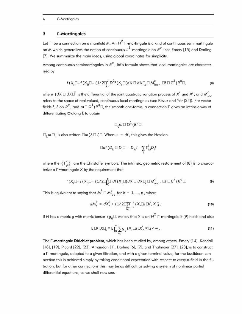
4 G-Martingales
3 Γ-Martingales
Let be a connection on a manifold M. An Γ-martingale is a kind of continuous semimartingale
on M which generalizes the notion of continuous martingale on : see Emery [15] and Darling
[7]. We summarize the main ideas, using global coordinates for simplicity.
Among continuous semimartingales in , ItÕs formula shows that local martingales are character-
ized by
, , (8)
where is the differential of the joint quadratic variation process of and , and
refers to the space of real-valued, continuous local martingales (see Revuz and Yor [24]). For vector
fields ξ, ζ on , and , the smooth one-forms, a connection Γ gives an intrinsic way of
differentiating ω along ξ to obtain
.
is also written . When , this gives the Hessian
where the are the Christoffel symbols. The intrinsic, geometric restatement of (8) is to charac-
terize a Γ−martingale X by the requirement that
, . (9)
This is equivalent to saying that for , where
. (10)
If N has a metric g with metric tensor , we say that X is an Γ-martingale if (9) holds and also
. (11)
The Γ-martingale Dirichlet problem, which has been studied by, among others, Emery [14], Kendall
[18], [19], Picard [22], [23], Arnaudon [1], Darling [6], [7], and Thalmaier [27], [28], is to construct
a Γ-martingale, adapted to a given filtration, and with a given terminal value; for the Euclidean con-
nection this is achieved simply by taking conditional expectation with respect to every σ-field in the fil-
tration, but for other connections this may be as difficult as solving a system of nonlinear partial
differential equations, as we shall now see.
Γ H2
L2
Rq
Rq
f Xt( ) f X0( )– 1 2⁄( ) D2f Xs( )
0
t∫ dX dX⊗( ) s– Mloc
c∈ f∀ C2
Rq( )∈
dX dX⊗( ) i jX
iX
jMloc
c
Rq ω Ω1
Rq( )∈
∇ ξω Ω1R
q( )∈
∇ ξω ζ⋅ ∇ω ξ ζ⊗( ) ω df=
∇ df Dk Di⊗( ) Dkif Γkij
Djfj
∑–=
Γ jki
f Xt( ) f X0( )– 1 2⁄( ) ∇ df Xs( )0
t∫ dX dX⊗( ) s– Mloc
c∈ f∀ C2
Rq( )∈
Mk
Mlocc∈ k 1 É p, ,=
dMtk
dXtk 1 2⁄( ) Γ i j
kXt( )
i j,∑ d X
iX
j,⟨ ⟩ t+=
gij( ) H2
E X X,⟨ ⟩ ∞ E gij Xt( )i j,∑ d X
iX
j,⟨ ⟩ t0
∞∫ ∞<≡

Taylor Approximation of a Gamma-Martingale Dirichlet Problem 5
4 Taylor Approximation of a Gamma-Martingale Dirichlet Problem
4.1 Condition for the Intrinsic Location Parameter
Consider a diffusion process on a p-dimensional manifold N with generator
where ∆ is the Laplace-Beltrami operator associated with the diffusion variance, and ξ is a vector field,
as in (7). The coordinate-free construction of the diffusion X, given a Wiener process W on , uses
the linear or orthonormal frame bundle: see Elworthy [13] p. 252. We suppose .
Also suppose is a Riemannian manifold, with Levi-Civita connection , and is a
map. The case of particular interest is when , , and the metric on N is a
Ògeneralized inverseÓ to in the sense of (4). The general case of is needed in the
context of nonlinear filtering: see Darling [8].
Following Emery, and Mokobodzki [16], we assert the following:
Axiom B: Any intrinsic location parameter for should be the initial value of an -
adapted -martingale on M, with terminal value .
This need not be unique, but we will specify a particular choice below. In the case where
does not depend on x, then the local connector Γ, given by (5), is zero, and is simply .
However our assertion is that, when Γ is not the Euclidean connection, the right measure of location
is , and not . We begin by indicating why an exact determination of is not compu-
tationally feasible in general.
4.2 Relationship with Harmonic Mappings
For simplicity of exposition, let us assume that there are diffeomorphisms and
which induce global coordinate systems for N and for M, respectively. By
abuse of notation, we will usually neglect the distinction between and , and write x
for both. is given by (2) and (5), and the local connector
comes from the Levi-Civita connection for .
In order to find , we need to construct an auxiliary adapted process , with values in
, such that the processes and satisfy the following system of forward-
backwards SDE:
, ; (12)
, . (13)
We also require that
. (14)
Xt 0 t δ≤ ≤, ξ 12---∆+
Rp
X0 x0 N∈=
M h,( ) Γ ψ:N M→C
2M N= ψ identity=
σ σ⋅ ψ:N M→
ψ Xδ( ) V0 ℑ tW
H2 Γ Vt 0 t δ≤ ≤, Vδ ψ Xδ( )=
σ σ⋅ x( )V0 E ψ Xδ( )[ ]
V0 E ψ Xδ( )[ ] V0
ϕ :N Rp→ ϕ:M R
q→x
1É x
p, , y1
É yq, ,
x N∈ ϕ x( ) Rp∈
Γ x( ) σ σ⋅( ) x( )( ) TxRp∈
Γ y( ) L TyRq
TyRq⊗ TyR
q;( )∈ M h,( )
Vt Zt L R
pTVt
Rq
; Xt Vt Zt,( )
Xt x0 b Xs( ) ds0
t∫ σ Xs( ) dWs0
t∫+ += 0 t δ≤ ≤
Vt ψ Xδ( ) Zs Wsdt
δ∫–
12--- Γ Vs( ) Zs Zs⋅( ) sd
t
δ∫+= 0 t δ≤ ≤
E hij Vs( ) Zs Zs⋅( ) i j
i j,∑ ds
0
δ∫ ∞<

6 Taylor Approximation of a Gamma-Martingale Dirichlet Problem
[Equation (13) and condition (14) together say that V is an -martingale, in the sense of (10)
and (11).] Such systems are treated by Pardoux and Peng [21], but existence and uniqueness of solu-
tions to (13) are outside the scope of their theory, because the coefficient is not Lipschitz
in z.
However consider the second fundamental form of a mapping . Recall that
may be expressed in local coordinates by:
(15)
for , . Let ξ be as in (7). Consider a system of quasilinear parabolic
PDE (a Òheat equation with driftÓ for harmonic mappings - see Eells and Lemaire [11], [12]) consist-
ing of a suitably differentiable family of mappings , for , such that
, , (16)
. (17)
For , the right side of (16) is . Following
the approach of Pardoux and Peng [21], ItÕs formula shows that
, (18)
(19)
solves (13). In particular . (A similar idea was used by Thalmaier [27].)
4.2.a Comments on the Local Solvability of (16) - (17)
Recall that the energy density of is given by
. (20)
Note, incidentally, that this formula still makes sense when is degenerate. In the case where
is non-degenerate and smooth, , and , the inverse function theorem
method of Hamilton [17], page 122, suffices to show existence of a unique smooth solution to (16) -
(17) when is sufficiently small. For a more detailed account of the properties of the solutions
when , see Struwe [26], pages 221 - 235. Whereas Eells and Sampson [10] showed the
existence of a unique global solution when has non-positive curvature, Chen and Ding [4]
showed that in certain other cases blow-up of solutions is inevitable. The case where is degener-
ate appears not to have been studied in the literature of variational calculus, and indeed is not within
the scope of the classical PDE theory of Ladyzenskaja, Solonnikov, and UralÕceva [20]. A probabilistic
construction of a solution, which may or may not generalize to the case where is degenerate,
H2 Γ
Γ v( ) z z⋅( )
∇ dφ C2 φ:N M→
∇ dφ x( ) L TxN TxN⊗ Tφ x( ) M;( )∈
∇ dφ x( ) v w⊗( ) D2φ x( ) v w⊗( ) Dφ x( ) Γ x( ) v w⊗( )– Γ y( ) Dφ x( ) v Dφ x( ) w⊗( )+=
v w,( ) TxRp
TxRp×∈ y φ x( )≡
u t .,( ) :N M→ t 0 δ,[ ]∈
t∂∂u du ξ⋅ 1
2--- ∇ du σ σ⋅( )+= 0 t δ≤ ≤
u 0 .,( ) ψ=
x N∈ du t .,( ) ξ x( )⋅ 12--- ∇ du t .,( ) σ σ⋅ x( )( )+ Tu t x,( ) M∈
Vt u δ t– Xt,( ) M∈=
Z t( ) du δ t– Xt,( ) σ Xt( )• L Rp
TVtM;
∈=
u δ x0,( ) V0=
ψ:N M→
e ψ( ) x( ) 12--- dψ dψ⊗ σ σ⋅( ) ψ x( )
2≡ 12--- hβγ ψ x( )( ) dψβ
x( ) dψγx( )⊗ σ σ⋅ x( )( )
β γ,∑=
σ σ⋅σ σ⋅ ξ 0= e ψ( ) volN( )d∫ ∞<
δ 0>dim N( ) 2=
M h,( )σ σ⋅
σ σ⋅

Taylor Approximation of a Gamma-Martingale Dirichlet Problem 7
will appear in Thalmaier [28]. Work by other authors, using Hrmander conditions on the generator
, is in progress. For now we shall merely assume:
Hypothesis I Assume conditions on ξ, , ψ, and h sufficient to ensure existence and unique-
ness of a solution , for some .
4.3 Definition: the Intrinsic Location Parameter
For , the intrinsic location parameter of is defined to be , where .
This depends upon the generator , given in (7), where ∆ may be degenerate; on the mapping
; and on the metric h for M. It is precisely the initial value of an -adapted -
martingale on M, with terminal value . However by using the solution of the PDE, we
force the intrinsic location parameter to be unique, and to have some regularity as a function of .
The difficulty with Definition 4.3 is that, in filtering applications, it is not feasible to compute solutions
to (16) and (17) in real time. Instead we compute an approximation, as we now describe.
4.4 A Parametrized Family of Heat Flows
Consider a parametrized family of equations of the type (16), namely
, , (21)
. (22)
Note that the case gives the system (16), while the case gives ,
where is the flow of the vector field ξ.
In a personal communication, Etienne Pardoux has indicated the possibility of a probabilistic con-
struction, involving the system of FBSDE (46) and (55), of a unique family of solutions for suffi-
ciently small , and for small time , based on the results of Darling [6] and methods of
Pardoux and Peng [21]. For now, it will suffice to replace Hypothesis I by the following:
Hypothesis II Assume conditions on ξ, , ψ, and h sufficient to ensure existence of and
such that there is a unique mapping from
to M satisfying (21) and (22) for each .
4.4.a Notation
For any vector field ζ on N, and any differentiable map into a manifold P, the Òpush-for-
wardÓ takes the value at ; likewise .
We must also assume for the following theorem that we have chosen a generalized inverse
to , in the sense of (3), so that we may construct a canonical sub-Riemannian
connection for , with respect to g.
We now state the first result, which will later be subsumed by Theorem 4.7.
ξ 12---∆+
σ σ⋅u t .,( ) :N M→ 0 t δ1≤ ≤, δ 1 0>
0 δ δ1≤ ≤ ψ Xδ( ) u δ x0,( ) x0 X0=
ξ 12---∆+
ψ:N M→ ℑ tW H
2 ΓVδ ψ Xδ( )=
x0
uγ 0 γ 1≤ ≤,
t∂∂u
γdu
γ ξ⋅ γ2--- ∇ du
γ σ σ⋅( )+= 0 t δ≤ ≤
uγ 0 .,( ) ψ=
γ 1= γ 0= u0
t x,( ) ψ φt x( )( )=
φt t 0≥,
uγ
γ 0≥ δ 0>
σ σ⋅ δ1 0>γ1 0> C
2 γ t x, ,( ) uγ
t x,( )→0 γ1,[ ] 0 δ1,[ ]× N× γ 0 γ1,[ ]∈
φ:N P→φ*ζ dφ ζ x( )⋅ TyP∈ y φ x( ) P∈≡ φ* ζ ζ′⊗( ) φ*ζ φ*ζ′⊗≡
g:T∗ N TN→ σ σ⋅∇° . .⟨ | ⟩

8 Taylor Approximation of a Gamma-Martingale Dirichlet Problem
4.5 Theorem (PDE Version)
Assume Hypothesis II, and that . Then, in the tangent space ,
(23)
where is the flow of the vector field ξ, , and
. (24)
In the special case where , , and , the right side of (23) simplifies to the
part in parentheses É.
4.5.a Definition
The expression (23) is called the approximate intrinsic location parameter in the tangent space
, denoted .
4.5.b Remark: How the Formula is Useful
First we solve the ODE for the flow of the vector field ξ, compute at
using (23) (or rather, using the local coordinate version (32)), then use the exponential map to
project the approximate location parameter on to N, giving
. (25)
Computation of the exponential map likewise involves solving an ODE, namely the geodesic flow on
M. In brief, we have replaced the task of solving a system of PDE by the much lighter task of solving
two ODEÕs and performing an integration.
4.6 The Stochastic Version
We now prepare an alternative version of the Theorem, in terms of FBSDE, in which we give a local
coordinate expression for the right side of (23). In this context it is natural to define a new parameter
ε, so that in (21). Instead of X in (12), we consider a family of diffusion processes
on the time interval , where has generator . Likewise V in (13) will
be replaced by a family of -martingales, with , and
. Note, incidentally, that such parametrized families of -martingales are also
treated in recent work of Arnaudon and Thalmaier [2], [3].
4.6.a Generalization to the Case of Random Initial Value
Suppose that, instead of as in (12), we have , where is a zero-
mean random variable in , independent of W, with covariance ; the last
expression means that, for any pair of cotangent vectors ,
0 δ δ1≤ ≤ Tψ xδ( ) M
γ∂∂ u
γ δ x0,( )γ 0=
∇ dψ xδ( ) φδ*Π
δ( ) ψ* ∇° dφδ x0( ) Πδ( ) φδ t–( )
*∇° dφt x0( ) Π td
0
δ∫– +
2-----------------------------------------------------------------------------------------------------------------------------------------------------------------------------------------=
φt t 0≥, xt φt x0( )≡
Π t φ s–( )*
. .⟨ | ⟩ xssd
0
t∫ Tx0
N Tx0N⊗∈≡
M N= ψ identity= h g=
Tψ xδ( ) M Ix0ψ Xδ( )[ ]
φt 0 t δ≤ ≤, ∂ uγ δ x0,( ) ∂γ⁄
γ 0=
expψ xδ( ) γ∂∂ u
γ δ x0,( )γ 0=
M∈
γ ε2=
Xε ε 0≥, 0 δ,[ ] X
ε ξ ε2∆ 2⁄+
Vε ε 0≥, H
2 Γ Vδε ψ Xδ
ε( )=
V0γ
uγ δ x0,( )= Γ
X0 x0 N∈= X0 expx0U0( )= U0
Tx0N Σ0 Tx0
N Tx0N⊗∈
β λ, Tx0
*N∈

Taylor Approximation of a Gamma-Martingale Dirichlet Problem 9
.
Now set up the family of diffusion processes with initial values
. (26)
Each -martingale is now adapted to the larger filtration .
In particular,
is now a random variable in depending on .
4.6.b Definition
In the case of a random initial value as above, the approximate intrinsic location parameter of
in the tangent space , denoted , is defined to be
. (27)
We will see in Section 6.3 below that this definition makes sense. This is the same as
,
and coincides with , given by (23), in the case where .
4.6.c Some Integral Formulas
Given the flow of the vector field ξ, the derivative flow is given locally by
, (28)
where , for . In local coordinates, we compute as a matrix, given by
.
Introduce the deterministic functions
, (29)
. (30)
Note, incidentally, that could be called the intrinsic variance parameter of .
E β U0⋅( ) λ U0⋅( )[ ] β λ⊗( ) Σ0⋅=
Xε ε 0≥,
X0ε
expx0εU0( )=
Γ Vtε 0 t δ≤ ≤, ℑ ˜
tW
ℑ tW σ U0( )∨ ≡
expψ xδ( )1–
V0ε
Tψ xδ( ) M U0
X0ψ Xδ( ) Tψ xδ( ) M Ix0 Σ0, ψ Xδ( )[ ]
ε2( )∂
∂ E expψ xδ( )1–
V0ε
ε 0=
γ∂∂ E expψ xδ( )
1–u
γ δ X0γ,
γ 0=
Ix0ψ Xδ( )[ ] Σ0 0=
φt 0 t δ≤ ≤,
τst
d φt φs1–•( ) xs( ) L Txs
N TxtN;( )∈≡
xs φs x( )= 0 s δ≤ ≤ τst
p p×
τst
exp Dξ xu( ) uds
t∫ =
χt φt s–( )*
. .⟨ | ⟩ xssd
0
t∫≡ τs
t σ σ⋅( ) xs( ) τst( )
Tsd
0
t∫ Txt
N TxtN⊗∈=
Ξt χt τ0t Σ0 τ0
t( )T
+ TxtN Txt
N⊗∈≡
Ξt Xt

10 Example of Computing an Intrinsic Location Parameter
4.7 Theorem (Local Cordinates, Random Initial Value Version)
Under the conditions of Theorem 4.5, with random initial value as in Section 4.6.a, the approxi-
mate intrinsic location parameter exists and is equal to the right side of (23), after
redefining
. (31)
In local coordinates, is given by
(32)
where , , and is given by (30).
4.7.a Remarks
• Theorem 4.7 subsumes Theorem 4.5, which corresponds to the case .
• In the special case where , , and , formula (32) reduces to:
. (33)
• In the filtering context [8], formulas (32) and (33) are of crucial importance.
5 Example of Computing an Intrinsic Location Parameter
The following example shows that Theorem 4.7 leads to feasible and accurate calculations.
5.1 Target Tracking
In target tracking applications, it is convenient to model target acceleration as an Ornstein-Uhlenbeck
process, with the constraint that acceleration must be perpendicular to velocity. Thus
must satisfy , and the trajectory must lie within a set on which is con-
stant. Therefore we may identify the state space N with , since the v-component lies on a
sphere, and the a-component is perpendicular to v, and hence tangent to .
Within a Cartesian frame, X is a process in with components V (velocity) and A (acceleration), and
the equations of motion take the nonlinear form:
. (34)
Here the square matrix consists of four matrices, λ and γ are constants, W is a three-dimen-
sional Wiener process, and if ,
, (35)
X0Ix0 Σ0, ψ Xδ( )[ ]
Π t Σ0 φ s–( )*
. .⟨ | ⟩ xssd
0
t∫+ Tx0
N Tx0N⊗∈≡
2Ix0 Σ0, ψ Xδ( )[ ]
J τ tδ
D2ξ xt( ) Ξt( ) Γ xt( ) σ σ⋅ xt( )( )–[ ] td
0
δ∫ D
2ψ xδ( ) Ξδ( ) Jτ0δΓ x0( ) Σ0( )– Γ yδ( ) JΞδJ
T( )+ +
yδ ψ xδ( )≡ J Dψ xδ( )≡ Ξt
Σ0 0=
M N= ψ identity= h g=
Ix0 Σ0, Xδ[ ] 12--- τ t
δD
2ξ xt( ) Ξt( ) Γ xt( ) σ σ⋅ xt( )( )–[ ] td0
δ∫ τ0
δΓ x0( ) Σ0( )– Γ xδ( ) Ξδ( )+ =
v a,( ) R3
R3×∈ v a⋅ 0= v
2
TS2
R6⊂
S2
R6
dVdA
03 3× I3ρ X( ) I3– λP V( )–
VA
dt 0γP V( ) dW t( )
+=
3 3×x
Tv
Ta
T,( )≡
ρ x( ) a2
v2⁄≡

Example of Computing an Intrinsic Location Parameter 11
, (36)
Note that is precisely the projection onto the orthogonal complement of v in , and has
been chosen so that .
5.2 Geometry of the State Space
The diffusion variance metric (2) is degenerate here; noting that , we find
. (37)
The rescaled Euclidean metric on is a generalized inverse to α in the sense of (3), since
. We break down a tangent vector ζ to into two 3-dimensional components and .
The constancy of implies that
. (38)
Referring to formula (5) for the local connector ,
, .
Taking first and second derivatives of the constraint , we find that
, . (39)
Using the last identity, we obtain from (5) the formula
, . (40)
In order to compute (32), note that, in particular,
. (41)
5.3 Derivatives of the Dynamical System
It follows from (7), (34), and (41) that the formula for the intrinsic vector field ξ is:
P v( ) I vvT
v2---------– L R
3R
3;( )∈≡
P v( ) R3 ρ x( )
d V A⋅( ) 0=
P2
P=
α σ σ⋅03 3× 03 3×
03 3× γ2P v( )
≡ ≡
g γ 2–I6= R
6
P2
P= R6 ζv ζa
v2
DP v( ) ηv1–
v2--------- ηvv
Tvηv
T+ =
Γ x( )
D g ζ( ) g ς( )⟨ | ⟩ η( ) 1–
γ2v
2---------------ζaT ηvv
Tvηv
T+( ) ςa= ζ ς η, ,( ) TxN TxN× TxN×∈
v a⋅ 0=
ζaTv ζv
Ta+ 0= ηa
Tζv ηvTζa+ 0=
Γ x( ) ζ ς⊗( ) S ζ ς⊗( ) v
2 v2--------------------------= S ζ ς⊗( )
ζaςaT ςaζa
T+
ζvςaT
– ςvζaT
–
≡
Γ x( ) σ σ⋅ x( )( ) γ2
v2--------- P v( )
0v 0
0= =

12 Example of Computing an Intrinsic Location Parameter
. (42)
Differentiate under the assumptions is constant and , to obtain
, . (43)
Differentiating (43) and using the identities (39),
. (44)
5.3.a Constraints in the Tangent Space of the State Manifold
Let us write a symmetric tensor in blocks as the matrix
,
where . Replacing by , and by , etc., in (44), we find that
. (45)
5.4 Ingredients of the Intrinsic Location Parameter Formula
Let be the inclusion of the state space into Euclidean . Thus in formula (32),
the local connector is zero on the target manifold, J is the identity, and is zero. When
is taken to be zero, the formula for the approximate intrinsic location parameter for
becomes:
,
where and are the velocity and acceleration components of , for , and
and are given by (28) and (29). A straightforward integration scheme for calculating
at the same time, using a discretization of , is:
,
,
ξ x( ) aρ x( ) v– λP v( ) a–
=
v2
v a⋅ 0=
Dξ x( ) ζ( ) 0 IλQ ρ– λP– 2Q–
ζv
ζa
= Q vaT
v2---------≡
D2ξ x( ) η ζ⊗( ) 2–
v2---------
0
ηaTζav ζvηa
T ηvζaT
+( ) a+=
χ TxN TxN⊗∈ 3 3×
χvv χva
χav χaa
χavT χva= ηvζa
T χva ηaTζa Tr χaa( )
D2ξ x( ) χ( ) 2–
v2---------
0Tr χaa( ) v χva χav+( ) a+
=
ψ:N R6→ N TS
2≅ R6
Γ .( ) D2ψ Σ0mδ Ix0
Xδ[ ]≡ Xδ
mt τutHu ud
0
t∫= Ht
1–
v02------------
0Tr χaa t( )( ) vt χva t( ) χav t( )+( ) at+
≡
vt at xt φt x( )≡ 0 t δ≤ ≤ τut
χt τut χt mt, ,( )
0 δ,[ ]
τut
exp t u–2
----------- Dξ xu( ) Dξ xt( )+[ ] ≈
χtt u–
2----------- σ σ⋅( ) xt( ) τu
t χut u–
2----------- σ σ⋅( ) xu( )+ τu
t( )T
+≈

Example of Computing an Intrinsic Location Parameter 13
.
Since the local connector is zero on the target manifold, geodesics are simply straight lines, and
is a suitable estimate of the mean position of .
5.5 Simulation Results
FIGURE 1 SIMULATIONS OF THE MEAN OF AN SDE, VERSUS ITS APPROXIMATE ILP
We created simulations of the process (34), with and , on the time inter-
val , which was discretized into 25 subintervals for integration purposes. In each case V and A
were initialized randomly, with magnitudes of 200 m/s and 50 m/s2, respectively. The plot shows the
x-component of acceleration (the other two are similar): the Ò+Ó signs represent the mean of the pro-
cess (34) over simulations , with bands showing plus and minus one standard error, the solid line
is the solution of the discretized ODE , and the circles denote the
approximate intrinsic location parameter (ILP). The reader will note that the ILP tracks the mean of
the process better than the ODE does.
mt τut
mut u–
2-----------Hu+
t u–2
-----------Ht+≈
xδ Ix0Xδ[ ]+ Xδ
0 5 10 15 20 25-12
-10
-8
-6
-4
-2
0
2x-acceleration: ODE "-", mean SDE +/- 1 s.e. "+", ILP "o"
104 λ 0.5= γ 5.2 103×=
0 1,[ ]
104
xt 0 t 1≤ ≤, dxt dt⁄ ξ xt( )=
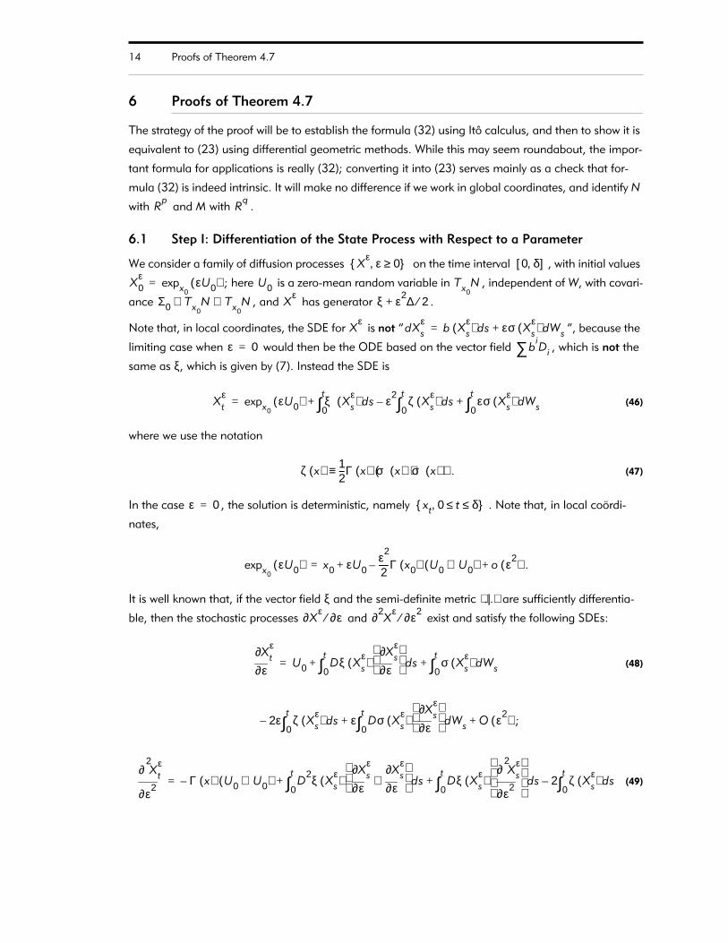
14 Proofs of Theorem 4.7
6 Proofs of Theorem 4.7
The strategy of the proof will be to establish the formula (32) using It calculus, and then to show it is
equivalent to (23) using differential geometric methods. While this may seem roundabout, the impor-
tant formula for applications is really (32); converting it into (23) serves mainly as a check that for-
mula (32) is indeed intrinsic. It will make no difference if we work in global coordinates, and identify N
with and M with .
6.1 Step I: Differentiation of the State Process with Respect to a Parameter
We consider a family of diffusion processes on the time interval , with initial values
; here is a zero-mean random variable in , independent of W, with covari-
ance , and has generator .
Note that, in local coordinates, the SDE for is not Ò Ò, because the
limiting case when would then be the ODE based on the vector field , which is not the
same as ξ, which is given by (7). Instead the SDE is
(46)
where we use the notation
. (47)
In the case , the solution is deterministic, namely . Note that, in local cordi-
nates,
.
It is well known that, if the vector field ξ and the semi-definite metric are sufficiently differentia-
ble, then the stochastic processes and exist and satisfy the following SDEs:
(48)
;
(49)
Rp
Rq
Xε ε 0≥, 0 δ,[ ]
X0ε
expx0εU0( )= U0 Tx0
N
Σ0 Tx0N Tx0
N⊗∈ Xε ξ ε2∆ 2⁄+
Xε
dXsε
b Xsε( ) ds εσ Xs
ε( ) dWs+=
ε 0= biDi∑
Xtε
expx0εU0( ) ξ Xs
ε( ) ds0
t∫ ε2 ζ Xs
ε( ) ds0
t∫– εσ Xs
ε( ) dWs0
t∫+ +=
ζ x( ) 12---Γ x( ) σ x( ) σ x( )⋅( )≡
ε 0= xt 0 t δ≤ ≤,
expx0εU0( ) x0 εU0
ε2
2-----Γ x0( ) U0 U0⊗( )– o ε2( )+ +=
. .⟨ | ⟩∂X
ε ∂ε⁄ ∂2X
ε ∂ε2⁄
ε∂∂Xt
ε
U0 Dξ Xsε( ) ε∂
∂Xsε
ds0
t∫ σ Xs
ε( ) dWs0
t∫+ +=
2ε ζ Xsε( ) ds
0
t∫– ε Dσ Xs
ε( ) ε∂∂Xs
ε
dWs0
t∫ O ε2( )+ +
ε2
2
∂
∂ Xtε
Γ x( ) U0 U0⊗( )– D2ξ Xs
ε( ) ε∂∂Xs
ε
ε∂∂Xs
ε
⊗
ds0
t∫ Dξ Xs
ε( )ε2
2
∂
∂ Xsε
ds0
t∫ 2 ζ Xs
ε( ) ds0
t∫–+ +=

Proofs of Theorem 4.7 15
,
where denotes terms of order ε. Define
, . (50)
Now (48) and (49) give:
, ; (51)
, (52)
,
where . Let be the two-parameter semigroup of deterministic matrices
given by (28), so that
; .
Then (51) becomes , which has a Gaussian solution
. (53)
Likewise (52) gives , whose
solution is
. (54)
6.2 Step II: Differentiation of the Gamma-Martingale with Respect to a Parameter
Consider the pair of processes obtained from (18) and (19), where u is replaced by . As
in the case where , gives an adapted solution to the backwards equation correspond-
ing to (13), namely
.
However the version of (19) which applies here is , so we may replace
by , and the equation becomes
2 Dσ Xsε( ) ε∂
∂Xsε
dWs0
t∫ O ε( )+ +
O ε( )
Λt ε∂∂Xt
ε
ε 0=
≡ Λt2( )
ε2
2
∂
∂ Xtε
ε 0=
≡
dΛt AtΛtdt σ xt( ) dWt+= Λ0 U0=
dΛt2( )
D2ξ xt( ) Λt Λt⊗( ) AtΛt
2( ) 2ζ xt( )–+[ ] dt 2Dσ xt( ) Λt( ) dWt+=
Λ02( ) Γ x0( ) U0 U0⊗( )–=
At Dξ xt( )≡ τst 0 s t δ≤,≤,
t∂∂τ t
s
τ tsAt–= τs
r τ trτs
t=
d τ t0Λt( ) τ t
0σ xt( ) dWt=
Λt τ0tU0 τ0
t τs0σ xs( ) Wsd
0
t∫+ τ0
tU0 τs
t σ xs( ) Wsd0
t∫+= =
d τ t0Λt
2( )( ) τ t0
D2ξ xt( ) Λt Λt⊗( ) 2ζ xt( )–[ ] dt 2τt
0Dσ xt( ) Λt( ) dWt+=
Λt2( ) τ0
t Γ x0( ) U0 U0⊗( )– τst
D2ξ xs( ) Λs Λs⊗( ) 2ζ xs( )–[ ] ds 2Dσ xs( ) Λs( ) dWs+
0
t∫+=
Vε
Zε,( ) u
ε
ε 1= Vε
Zε,( )
Vtε ψ Xδ
ε( ) ZsεdWst
δ∫–
12--- Γ Vs
ε( ) Zsε
Zsε⋅( ) sd
t
δ∫+=
Ztε
Duε δ t– Xt,( ) εσ Xt( )=
Zsε εZs
ε
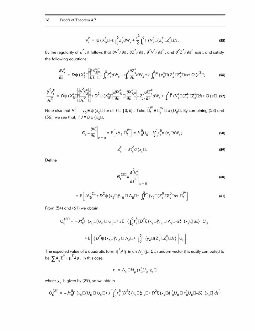
16 Proofs of Theorem 4.7
. (55)
By the regularity of , it follows that , , , and exist, and satisfy
the following equations:
; (56)
. (57)
Note also that for all . Take . By combining (53) and
(56), we see that, if ,
; (58)
. (59)
Define
(60)
(61)
From (54) and (61) we obtain:
.
The expected value of a quadratic form in an random vector η is easily computed to
be . In this case,
,
where is given by (29), so we obtain
Vtε ψ Xδ
ε( ) ε ZsεdWst
δ∫–
ε2
2----- Γ Vs
ε( ) Zsε
Zsε⋅( ) sd
t
δ∫+=
uε ∂V
ε ∂ε⁄ ∂Zε ∂ε⁄ ∂2
Vε ∂ε2⁄ ∂2
Zε ∂ε2⁄
ε∂∂Vt
ε
Dψ Xδε( ) ε∂
∂Xδε
ZsεdWst
δ∫– ε ε∂
∂Zsε
dWst
δ∫– ε Γ Vs
ε( ) Zsε
Zsε⋅( ) sd
t
δ∫ O ε2( )+ +=
ε2
2
∂
∂ Vtε
Dψ Xδε( )
ε2
2
∂
∂ Xδε
D2ψ Xδ
ε( ) ε∂∂Xδ
ε
ε∂∂Xδ
ε
⊗
2 ε∂∂Zs
ε
dWst
δ∫– Γ Vs
ε( ) Zsε
Zsε⋅( ) sd
t
δ∫ O ε( )+ + +=
Vt0
yδ ψ xδ( )≡= t 0 δ,[ ]∈ ℑ ˜tW
ℑ tW σ U0( )∨≡
J Dψ xδ( )≡
Θt ε∂∂Vt
ε
ε 0=
E JΛδ ℑ tW
Jτ0δU0 J τs
δσ xs( ) Wsd0
t∫+= =≡
Zs0
Jτsδσ xs( )=
Θt2( )
ε2
2
∂
∂ Vtε
ε 0=
≡
E JΛδ2( )
D2ψ xδ( ) Λδ Λδ⊗( ) Γ yδ( ) Zs
0Zs
0⋅( ) sdt
δ∫+ + ℑ t
W=
Θ02( )
Jτ0δΓ x0( ) U0 U0⊗( )– JE τs
δD
2ξ xs( ) Λs Λs⊗( ) 2ζ xs( )–[ ] ds0
δ∫ U0+=
E D2ψ xδ( ) Λδ Λδ⊗( ) Γ yδ( ) Zs
0Zs
0⋅( ) sd0
δ∫+ U0+
ηTAη Np µ Σ,( )
AijΣi j∑ µT
Aµ+
η Λ s Np τ0tU0 χs,( )∼=
χt
Θ02( )
Jτ0δΓ x0( ) U0 U0⊗( )– J τs
δD
2ξ xs( ) χs( ) D2ξ xs( ) τ0
sU0 τ0
sU0⊗( ) 2ζ xs( )–+[ ] ds
0
δ∫+=

Proofs of Theorem 4.7 17
. (62)
6.3 Step III: A Taylor Expansion Using the Exponential Map
Let , and define . Referring to (27), we are seeking . It
follows immediately from the geodesic equation that
, (63)
It follows from (58) and (62) that
.
A Taylor expansion based on (63) gives
.
Taking expectations, and recalling that has mean zero and covariance , we
obtain
It follows that , and hence that
where . If we write
, (64)
then the formula becomes
D2ψ xδ( ) χδ( ) D
2ψ xδ( ) τ0δU0 τ0
δU0⊗( ) Γ yδ( ) JχδJ
T( )+ + +
yδ ψ xδ( )≡ β ε( ) E expyδ
1–V0
ε≡ ∂β δ⁄ ε2ε 0=
D expy( ) 1–y( ) w( ) w= D
2expy( ) 1–
y( ) v w⊗( ) Γ y( ) v w⊗( )=
V0ε
yδ εJτ0δU0
ε2
2-----Θ0
2( )o ε2( )+ + +=
expyδ
1–V0
εV0
εyδ–
12---Γ yδ( ) V0
εyδ–( ) V0
εyδ–( )⊗( ) o V0
εyδ–
2
+ +=
εJτ0δU0
ε2
2----- Θ0
2( ) Γ yδ( ) Jτ0δU0 Jτ0
δU0⊗( )+ o ε2( )+ +=
U0 Σ0 Tx0N Tx0
N⊗∈
β ε( ) ε2
2----- E Θ0
2( )[ ] Γ yδ( ) Jτ0δΣ0 Jτ0
δ( )T
+ o ε2( )+=
εddβ
ε 0=
0=
ε2( )∂
∂ β ε( ) ε 0=12---
ε2
2
d
d β
ε 0=
=
12--- E Θ0
2( )[ ] Γ yδ( ) Jτ0δΣ0 Jτ0
δ( )T
+ =
12--- J τs
δD
2ξ xs( ) χs( ) Γ xs( ) σ σ⋅ xs( )( )–[ ] ds0
δ∫ D
2ψ xδ( ) χδ( ) Γ yδ( ) JχδJT( )+ +=
J τsδD
2ξ xs( ) Σs( ) ds0
δ∫ Jτ0
δΓ x0( ) Σ0( )– D2ψ xδ( ) Σδ( ) Γ yδ( ) JΣδJ
T( )+ + +
Σs τ0s Σ0 τ0
s( )T
≡
Ξs χs Σs+≡
18 Proofs of Theorem 4.7
.
This establishes the formula (32). ×
6.4 Step IV: Intrinsic Version of the Formula
It remains to prove that (23), with as in (31), is the intrinsic version of (32). We abbreviate here by
writing as . By definition of the flow of ξ,
,
and so, differentiating with respect to x, and exchanging the order of differentiation,
(65)
or, by analogy with (28), taking ,
; . (66)
Since , we have , which upon differentiation yields
,
which gives
; . (67)
A further differentiation of (65) when ψ is the identity yields
. (68)
Combining (67) and (68), we have
. (69)
The formula (15) for can be written as
12--- J τs
δD
2ξ xs( ) Ξs( )[ ] ds0
δ∫ D
2ψ xδ( ) Ξδ( ) Γ yδ( ) JΞδJT( )+ +
12---J τs
δΓ xs( ) σ σ⋅ xs( )( ) ds0
δ∫ τ0
δΓ x0( ) Σ0( )+ –
Π t
ψ φt• ψ t
t∂∂ ψt x0( ) dψ ξ• φt x0( )( )=
t∂∂ Dψt x0( ) D
t∂∂ ψt x0( )
=
θst
Dψt s– xs( )≡ Dψ xt( ) D φt φs1–•( ) xs( )• Dψ xt( ) τs
t= =
t∂∂τs
t
Dξ xt( ) τst
=t∂
∂θst
Dψ xt( ) Dξ xt( ) τst•=
τ tδτ0
t τ0δ
= θtδτ0
tDψ xδ( ) τ t
δτ0t θ0
δ= =
t∂∂θt
δ
τ0t θt
δt∂
∂τ0t
– θtδDξ xt( ) τ0
t–= =
t∂∂τ t
δ
τ tδDξ xt( )–=
t∂∂θt
δ
θtδDξ xt( )–=
t∂∂ D
2φt x0( ) v w⊗( ) D
2ξ xt( ) τ0tv τ0
tw⊗( ) Dξ xt( ) D
2φt x0( ) v w⊗( )+=
t∂∂ θt
δD
2φt x0( )( ) θtδDξ xt( ) D
2φt x0( )– θtδ
D2ξ xt( ) τ0
t.( ) τ0
t.( )⊗( ) Dξ xt( ) D
2φt x0( )+ +=
t∂∂ θt
δD
2φt x0( )( ) v w⊗( ) θtδD
2ξ xt( ) τ0tv τ0
tw⊗( )=
∇° dφt

Proofs of Theorem 4.7 19
(70)
It is clear that
.
Hence from (69) and (70) it follows that
. (71)
The last term in (71) can be written, using (66), as
, (72)
for . We will replace by
(73)
where . Observe that
. (74)
Moreover from (74) and (66), it is easily checked that
. (75)
It follows from (71) - (75) that
.
∇° dφt x0( ) v w⊗( ) D2φt x0( ) v w⊗( ) τ0
t Γ x0( ) v w⊗( )– Γ xt( ) τ0tv τ0
tw⊗( )+=
t∂∂ θt
δτ0t Γ x0( )( )
t∂∂ θ0
δΓ x0( )( ) 0= =
t∂∂ ψδ t–( )
*∇° dφt x0( ) v w⊗( )
t∂∂ θt
δD
2φt x0( ) v w⊗( ) Γ xt( ) τ0tv τ0
tw⊗( )+[ ] =
θtδD
2ξ xt( ) τ0tv τ0
tw⊗( )
t∂∂ θt
δΓ xt( ) τ0tv τ0
tw⊗( ) +=
t∂∂ θt
δΓ xt( ) τ 0tv τ0
tw⊗( ) θt
δΓ xt( ) Dξ xt( ) τ0tv τ0
tw⊗ τ 0
tv Dξ xt( ) τ
0tw⊗+
+
v w⊗ Tx0N Tx0
N⊗∈ v w⊗
Π t τ t0Ξt τ t
0( )T
≡ Σ0 τs0 σ σ⋅( ) xs( ) τs
0( )T
sd0
t∫+ Tx0
N Tx0N⊗∈=
Ξt χt τ0t Σ0 τ0
t( )T
+≡
τ0t Π t τ0
t( )T
Ξt= TxtN Txt
N⊗∈
td
dΞt σ σ⋅( ) xt( ) Dξ xt( ) Ξt Ξt Dξ xt( ) T
+ +=
t∂∂ ψδ t–( )
*∇° dφt x0( ) Π t( ) ψ δ t–( )
*∇° dφt x0( )
td
dΠ t
–t∂
∂ ψδ t–( )*∇° dφt x0( ) Π t( )=
θtδD
2ξ xt( )t∂
∂ θtδΓ xt( ) + Ξt( ) θt
δΓ xt( ) Dξ xt( ) Ξt Ξt Dξ xt( )( ) T+[ ]+=
θtδD
2ξ xt( )t∂
∂ θtδΓ xt( ) + Ξt( ) θt
δΓ xt( )td
dΞt σ σ⋅( ) xt( )–
+=
θtδD
2ξ xt( ) Ξt( ) θtδΓ xt( ) σ σ⋅( ) xt( )( )–
t∂∂ θt
δΓ xt( ) Ξt( ) +=

20 The Canonical Sub-Riemannian Connection
Since , it follows upon integration from 0 to δ that in ,
. (76)
However the formula (15) for can be written as
. (77)
where , and . We take , and add (76) and (77):
.
The equivalence of (23) and (32) is established, completing the proofs of Theorems 4.5 and 4.7. ×
7 The Canonical Sub-Riemannian Connection
The purpose of this section is to present a global geometric construction of a torsion-free connection
on the tangent bundle which preserves, in some sense, a semi-definite metric on the
cotangent bundle induced by a section σ of of constant rank. In other words,
we assume that there exists a rank r vector bundle , a sub-bundle of the tangent bundle, such
that for all .
Given such a section σ, we obtain a vector bundle morphism by the formula
, , (78)
where is the canonical isomorphism induced by the Euclidean inner product. The rela-
tion between α and is that, omitting x,
, . (79)
7.1 Lemma
Under the constant-rank assumption, any Riemannian metric on N induces an orthogonal splitting of
the cotangent bundle of the form
, (80)
where is a rank r sub-bundle of the cotangent bundle on which is non-degenerate. There
exists a vector bundle isomorphism such that , and
is a generalized inverse to , in the sense that
∇° dφ0 0= Tψ xδ( ) M
ψ*∇° dφδ x0( ) Πδ( ) ψδ t–( )*
∇° dφt x0( )( ) Π td0
δ∫– =
Dψ xδ( ) τ tδ
D2ξ xt( ) Ξt( ) Γ xt( ) σ σ⋅( ) xt( )( )–[ ] td
0
δ∫ Γ xδ( ) Ξδ( ) τ0
δΓ x0( ) Ξ0( )–+
∇ dψ xδ( ) v w⊗( )
D2ψ xδ( ) v w⊗( ) JΓ xδ( ) v w⊗( )– Γ yδ( ) Jv Jw⊗( )+
yδ ψ xδ( )≡ J Dψ xδ( )≡ v w⊗ Ξ δ TxδN Txδ
N⊗∈=
J τ tδ
D2ξ xt( ) Ξt( ) Γ xt( ) σ σ⋅( ) xt( )( )–[ ] td
0
δ∫ D
2ψ xδ( ) Ξδ( ) Jτ0δΓ x0( ) Ξ0( )– Γ yδ( ) JΞδJ
T( )+ +
∇ dψ xδ( ) φδ( )*Π
δ( ) ψ* ∇° dφδ x0( ) Πδ( ) φδ t–( )
*∇° dφt x0( )( ) Π td
0
δ∫– +=
∇° TN C2
. .⟨ | ⟩T∗ N Hom R
pTN;( )
E N→Ex range σ x( )( ) TxN⊆= x N∈
α :T∗ N TN→
α x( ) σ x( ) ι• σ x( ) ∗•≡ x N∈
ι : Rp( ) ∗
Rp→. .⟨ | ⟩
µ α λ( )⋅ µ λ⟨ | ⟩≡ µ T∗ N∈∀
Tx∗ N Ker α x( )( ) Fx⊕=
F N→ . .⟨ | ⟩α° :T∗ N TN→ Fx Ker α° x( ) α x( )–( )=
α° x( ) 1– α x( )

The Canonical Sub-Riemannian Connection 21
.
Proof: For any matrix A, , and so . It fol-
lows that
.
Given a Riemannian metric g on N (which always exists), let be the dual metric on the cotan-
gent bundle. Define
.
We omit the proof that is a vector bundle. Since , it follows that
; since the rank of is r, we see that for all non-zero . This shows that
is non-degenerate on the sub-bundle .
Now (80) results from the orthogonal decomposition of with respect to . Hence an arbi-
trary can be decomposed as , with and . The metric
induces a vector bundle isomorphism , namely
, .
Now define by
.
It is clearly linear, and a vector bundle morphism. Since β is injective,
,
which shows that . To show is an isomorphism, it suffices to show that
whenever . When , non-degeneracy of implies that
.
On the other hand when , and , non-degeneracy of on implies that
.
Hence is a vector bundle isomorphism as claimed. The generalized inverse property
follows from the fact that . ×
7.2 Proposition
Suppose σ is a constant-rank section of , inducing a semi-definite metric on
and a vector bundle morphism as in (78) and (79). Suppose furthermore that
is a vector bundle isomorphism such that , as in
α x( ) α° x( ) 1–• α x( )• α x( )=
range A( ) range AAT( )= range α x( )( ) range σ x( )( )=
dim Ker α x( )( ) p dimEx– p r–= =
. .⟨ | ⟩°
Fx θ Tx∗ N∈ : θ λ⟨ | ⟩ x° 0= λ Ker α x( )( )∈∀ ≡
F N→ dim Ker α x( )( ) p r–=
dimFx r= . .⟨ | ⟩ θ θ⟨ | ⟩ 0> θ Fx∈. .⟨ | ⟩ F N→
Tx∗ N . .⟨ | ⟩°
λ Tx∗ N∈ λ λ 0 λ1⊕= λ0 Ker α x( )( )∈ λ 1 Fx∈
. .⟨ | ⟩° β :T∗ N TN→
µ β λ( )⋅ µ λ⟨ | ⟩°≡ µ T∗ N∈∀
α° :T∗ N TN→
α° λ( ) β λ0( ) α λ 1( )+≡
λ Tx∗ N∈ : α° λ( ) α λ( )= λ 0 λ1⊕ Tx
∗ N∈ : β λ0( ) 0= Fx= =
Fx Ker α° x( ) α x( )–( )= α°α° λ( ) 0≠ λ 0≠ λ0 0≠ . .⟨ | ⟩°
λ0 α° λ( )⋅ λ0 λ0⟨ | ⟩° λ 0 λ1⟨ | ⟩+ λ0 λ0⟨ | ⟩° 0≠= =
λ0 0= λ1 0≠ . .⟨ | ⟩ F N→
λ1 α° λ( )⋅ λ1 α λ 1( )⋅ λ1 λ1⟨ | ⟩ 0≠= =
α° :T∗ N TN→α x( ) α° x( ) 1–• α x( )• λ( ) λ1=
Hom Rp
TN;( ) . .⟨ | ⟩ T∗ N
α :T∗ N TN→α° :T∗ N TN→ α x( ) α° x( ) 1–• α x( )• α x( )=

22 The Canonical Sub-Riemannian Connection
Lemma 7.1. Then admits a canonical sub-Riemannian connection for , with respect to
, which is torsion-free, and such that the dual connection preserves in the following sense:
for vector fields V in the range of α, and for 1-forms which lie in the sub-bundle ,
. (81)
[Here .] For any 1-forms , and corresponding vector fields
, , ,
the formula for is:
. (82)
7.2.a Expression in Local Cordinates
Take local cordinates for N, so that is represented by a matrix , and by a
matrix , where by Lemma 7.2,
.
Take , , and in (82), so that , etc.; (82) becomes
. (83)
When is non-degenerate, then , and (83) reduces to the standard formula for the
Levi-Civita connection for g, namely
.
7.2.b Remark
A similar construction appears in formula (2.2) of Strichartz [25], where he cites unpublished work of
N. C. Gnther.
7.2.c Proof of Proposition 7.2
First we check that the formula (82) defines a connection. The R-bilinearity of is
immediate. To prove that for all , we replace W by and λ
by on the right side of (82), and the required identity holds. Verification that (82) is torsion-free is
likewise a straightforward calculation.
Next we shall verify (81). By (79), and the definition of duality, taking ,
.
Switch µ and λ in the last expression to obtain:
TN ∇° . .⟨ | ⟩α° ∇ˆ . .⟨ | ⟩
θ λ, F Ker α° α–( )≡
V θ λ⟨ | ⟩ ∇ˆ Vθ λ⟨ | ⟩ θ ∇ˆ Vλ⟨ | ⟩+=
∇ Zθ W⋅ Z θ W⋅( ) θ ∇° ZW⋅–= θ µ λ, ,
Y α° θ( )≡ Z α° µ( )≡ W α° λ( )≡
∇°
µ ∇° YW⋅ 12--- Y λ µ⟨ | ⟩ W µ θ⟨ | ⟩ Z θ λ⟨ | ⟩– λ Z Y,[ ]⋅ µ Y W,[ ]⋅ θ W Z,[ ]⋅–+ + + ≡
α° x( ) 1–glm( ) α x( )
α jk( )
α jkgkrα
rm
k r,∑ α jm
=
Y ∂ ∂xi⁄≡ W ∂ ∂xj⁄≡ Z ∂ ∂xk⁄≡ µ gksdxs∑=
Γ i js
gsks∑ 1
2---
xi∂∂ gjrα
rsgsk( )
xj∂∂ girα
rsgsk( )
xk∂∂ girα
rsgsj( )–+
r s,∑=
. .⟨ | ⟩ gjrαrs
r∑ δj
s=
Γ i js
gsks∑ 1
2---
xi∂∂gjk
xj∂∂gik
xk∂∂gij–+
=
Y W,( ) ∇° YW→∇° YfW f∇° YW Yf( ) W+= f C
∞N( )∈ fW
fλ
V α θ( )≡
µ ∇° Vα λ( )⋅ V µ α λ( )⋅( ) ∇ Vµ α λ( )⋅– V λ µ⟨ | ⟩ λ ∇ˆ Vµ⟨ | ⟩–= =

Future Directions 23
.
Taking and , we see that
. (84)
In terms of the splitting of Lemma 7.1, we may write , etc., and
we find that, if , then , etc. It follows from (82) that
;
.
To prove (81), we can assume , and now the right side of (84) becomes
,
as desired. ×
8 Future Directions
We would like to find out under what conditions on ξ, , ψ, and h the system of PDE (16) - (17)
has a unique solution for small time, other than the well-known case where is non-degenerate,
and ; likewise for the parametrized family (21) - (22). It is likely that the conditions will involve
the energy of the composite maps . Both stochastic and geometric methods should
be considered. Another valuable project would be to derive bounds on the error of approximation
involved in the linearization used in Theorem 4.7. This is likely to involve the curvature under the diffu-
sion variance semi-definite metric Ð see Darling [9].
Acknowledgments: The author thanks the Statistics Department at the University of California at Berkeley for its hospitality during the writing of this article, Anton Thalmaier for allowing access to unpublished work, and James Cloutier, James Eells, Etienne Pardoux, and Richard Schoen for their advice.
9 References
[1] M. Arnaudon. Esprances conditionelles et C-martingales dans les varits. Sminaire de Probabilit XXVIII, Lecture Notes in Mathematics 1583, (1994) 300-311.
[2] M. Arnaudon, A. Thalmaier. Stability of stochastic differential equations in manifolds. Smi-naire de Probabilits XXXI, Lecture Notes in Mathematics (1997, to appear).
[3] M. Arnaudon, A. Thalmaier. Complete lifts of connections and stochastic Jacobi fields. Uni-versitt Regensburg Preprint (1997).
[4] Y.-M. Chen, W.-Y. Ding. Blow-up and global existence for heat flows of harmonic maps. Invent. Math. 99, (1990) 567-578.
[5] R. W. R. Darling. Differential Forms and Connections. Cambridge University Press, 1994.[6] R. W. R. Darling. Constructing gammaÐmartingales with prescribed limit using backwards
SDE. Annals of Probability, 23 (1995), 1234-1261.
λ ∇° Vα µ( )⋅ V λ µ⟨ | ⟩ µ ∇ˆ Vλ⟨ | ⟩–=
U α µ( )≡ S α λ( )≡
V λ µ⟨ | ⟩ λ ∇ˆ Vµ⟨ | ⟩– µ ∇ Vλ⟨ | ⟩– µ ∇° VS⋅ λ ∇° VU⋅ V λ µ⟨ | ⟩–+=
Tx∗ N Ker α x( )( ) Fx⊕= θ θ0 θ1+≡
V α θ( )≡ V α θ1( ) α° θ1( )= =
µ1 ∇° VS⋅ 12--- V λ1 µ1⟨ | ⟩ S µ1 θ1⟨ | ⟩ U θ1 λ1⟨ | ⟩– λ1 U V,[ ]⋅ µ1 V S,[ ]⋅ θ1 S U,[ ]⋅–+ + + ≡
λ1 ∇° VU⋅ 12--- V λ1 µ1⟨ | ⟩ U λ1 θ1⟨ | ⟩ S θ1 µ1⟨ | ⟩– µ1 S V,[ ]⋅ λ1 V U,[ ]⋅ θ1 U S,[ ]⋅–+ + + ≡
λ0 µ0 0= =
µ1 ∇° VS⋅ λ1 ∇° VU⋅ V λ1 µ1⟨ | ⟩–+ 0=
σ σ⋅σ σ⋅
ξ 0=
ψ φt• 0 t δ≤ ≤,
24 References
[7] R. W. R. Darling. Martingales on noncompact manifolds: maximal inequalities and prescribed limits. Ann. de lÕInstitut H. Poincar B, 32, No. 4 (1996), 1-24.
[8] R. W. R. Darling. Geometrically intrinsic nonlinear recursive filters I: algorithms. Preprint (1997), available as No. 494 at http://www.stat.berkeley.edu/tech-reports/
[9] R. W. R. Darling. Geometrically intrinsic nonlinear recursive filters II: foundations. Preprint (1998), available as No. 512 at http://www.stat.berkeley.edu/tech-reports/
[10] J. Eells, J. H. Sampson. Harmonic mappings of Rimeannian manifolds. Amer. J. Math 86 (1964), 109-160.
[11] J. Eells, L. Lemaire. A report on harmonic maps. Bull. London Math. Soc. 10 (1978), 1Ð68.[12] J. Eells, L. Lemaire. Another report on harmonic maps. Bull. London Math. Soc. 20 (1988),
385Ð524.[13] K. D. Elworthy. Stochastic Differential Equations on Manifolds. Cambridge University Press,
1982.[14] M. Emery. Convergence des martingales dans les varits. Colloque en lÕhommage de Lau-
rent Schwartz, Vol. 2, Astrisque 132, Socit Mathmatique de France (1985), 47Ð63.[15] M. Emery. Stochastic Calculus on Manifolds. Springer, Berlin, 1989. (Appendix by P. A.
Meyer).[16] M. Emery, G. Mokobodzki. Sur le barycentre dÕune probabilit dans une varitÕ. Sminaire
de Probabilits XXV, Lecture Notes in Mathematics 1485 (1991), 220Ð233.[17] R. S. Hamilton. Harmonic maps of manifolds with boundary. Lecture Notes in Mathematics
471 (1975).[18] W. S. Kendall. Probability, convexity, and harmonic maps with small image I: uniqueness and
fine existence. Proc. London Math. Soc. 61 (1990), 371Ð406.[19] W.S. Kendall. Probability, convexity, and harmonic maps II: smoothness via probabilistic gra-
dient inequalities. Journal of Functional Analysis 126 (1994), 228-257.[20] O. A. Ladyzenskaja, V. A. Solonnikov, N. N. UralÕceva. Linear and Quasilinear Equations of
Parabolic Type. Translations of Math. Monongraphs 23, American Mathematical Society, Providence, 1968.
[21] E. Pardoux, S. Peng. Backward stochastic differential equations and quasilinear parabolic partial differential equations, in Stochastic Partial Differential Equations and Their Applica-tions, B.L. Rozowskii, R.B. Sowers (eds.), Lecture Notes in Control and Information Sciences 176, Springer-Verlag, Berlin, 1992.
[22] J. Picard. Martingales on Riemannian manifolds with prescribed limit. J. Functional Analysis 99 (1991), 223Ð261.
[23] J. Picard. Barycentres et martingales sur une varit. Annales de LÕInstitut Henri Poincar B, 30 (1994), 647-702.
[24] D. Revuz, M. Yor. Continuous Martingales and Brownian Motion. SpringerÐVerlag, Berlin 1991.
[25] R. Strichartz. Sub-Riemannian geometry. Journal of Differential Geometry 24 (1986), 221 - 263; corrections 30 (1989), 595 - 596.
[26] M. Struwe: Variational Methods: Applications to Nonlinear Partial Differential Equations and Hamiltonian Systems. Springer-Verlag, Berlin, 1996.
[27] A. Thalmaier. Brownian motion and the formation of singularities in the heat flow for har-monic maps. Probability Theory and Related Fields 105 (1996), 335-367.
[28] A. Thalmaier. Martingales on Riemannian manifolds and the nonlinear heat equation. Uni-versity of Regensburg Preprint (1996).