Embed Size (px)
Citation preview

Intro to Inverse Problems
in Exploration Seismology
M. D. Sacchi
Department of Physics
Institute for Geophysical Research
University of Alberta
PIMS Summer School 06 - Inversion and Imaging
M.D.Sacchi 1

Contact:
M.D.Sacchi
Notes:
www-geo.phys.ualberta.ca/~ sacchi/slides.pdf
M.D.Sacchi 2

• Inverse Problems in Geophysics
• Reflection Seismology
• Introduction to Inverse Problems
• Inverse Problems in Reflection Seismology
M.D.Sacchi 3

Geophysics
• In Geophysics old and new physical theories
are used to understand processes that occur in
the Earth’s interior (i.e., mantle convection,
Geo-dynamo, fluid flow in porous media, etc)
and to estimate physical properties that
cannot be measured in situ (i.e., density,
velocity, conductivity, porosity, etc)
M.D.Sacchi 4

What makes Geophysics different from other
geosciences?
• Physical properties in the Earth’s interior are
retrieved from indirect measurements
(observations)
• Physical properties are continuously
distributed in a 3D volume, observations are
sparsely distributed on the surface of the
earth.
M.D.Sacchi 5
How do we convert indirect measurements
into material properties ?
• Brute force approach
• Inverse Theory
• A combination of Signal Processing and
Inversion Techniques
M.D.Sacchi 6

Another aspect that makes Geophysics unique is
the problem of non-uniqueness
Toy Problem:
m1 + m2 = d
given one observation d find m1 and m2
M.D.Sacchi 7

Dealing with non-uniqueness
Non-uniqueness can be diminished by
incorporating into the problem:
• Physical constraints
Velocities are positives
Causality
• Non-informative priors
Bayesian inference, MaxEnt priors
• Results from Lab experiments
• Common sense = Talk to the Geologists a
aThey can understand the complexity involved in defin-
ing an Earth model.
M.D.Sacchi 8

Reflection Seismology involves solving problems
in the following research areas:
Wave Propagation Phenomena: we deal
with waves
Digital Signal Processing (DSP): large
amounts of data in digital format, Fast
Transforms are needed to map data to
different domains
Computational Physics/Applied Math:
large systems of equations, FDM, FEM,
Monte Carlo methods, etc
High Performance Computing (HPC):
large data sets (>Terabytes), large systems of
equations need to be solved again and again
and again
Inverse Problems: to estimate an Earth
model
Statistics: source estimation problems, to
deal with signals in low SNR environments,
risk analysis, etc
M.D.Sacchi 9
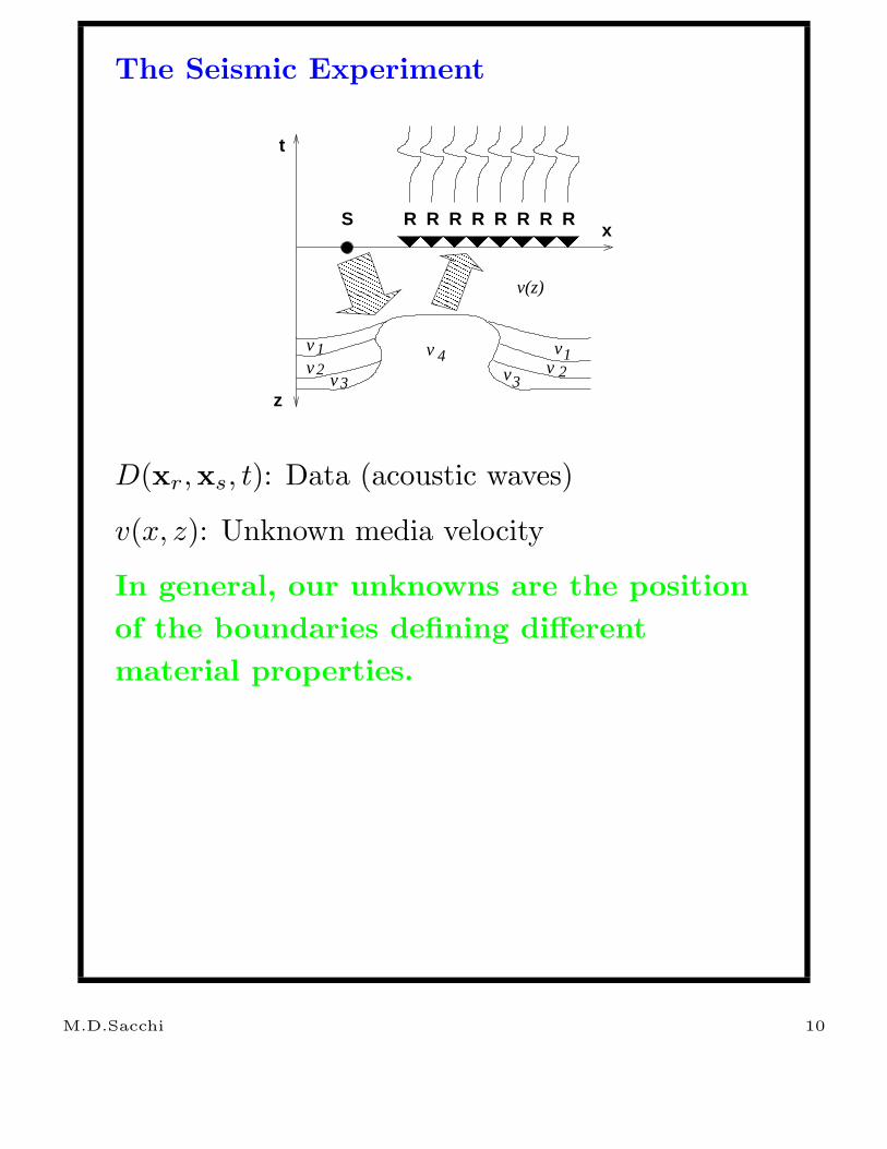
The Seismic Experiment
������������������������������������������������������������������������������
������������������������
�������������������������������������������������
�������������������������������������������������
� � � � � � � � � � � � � �
����������������������������������� ���
���������������������������������������
������������������ x
S RRRRR
z
t
R RR
v(z)
v 4v 1v 2
v 3
v12v3
v
D(xr,xs, t): Data (acoustic waves)
v(x, z): Unknown media velocity
In general, our unknowns are the position
of the boundaries defining different
material properties.
M.D.Sacchi 10

The Seismic Experiment :/eps: Command
not found.
M.D.Sacchi 11
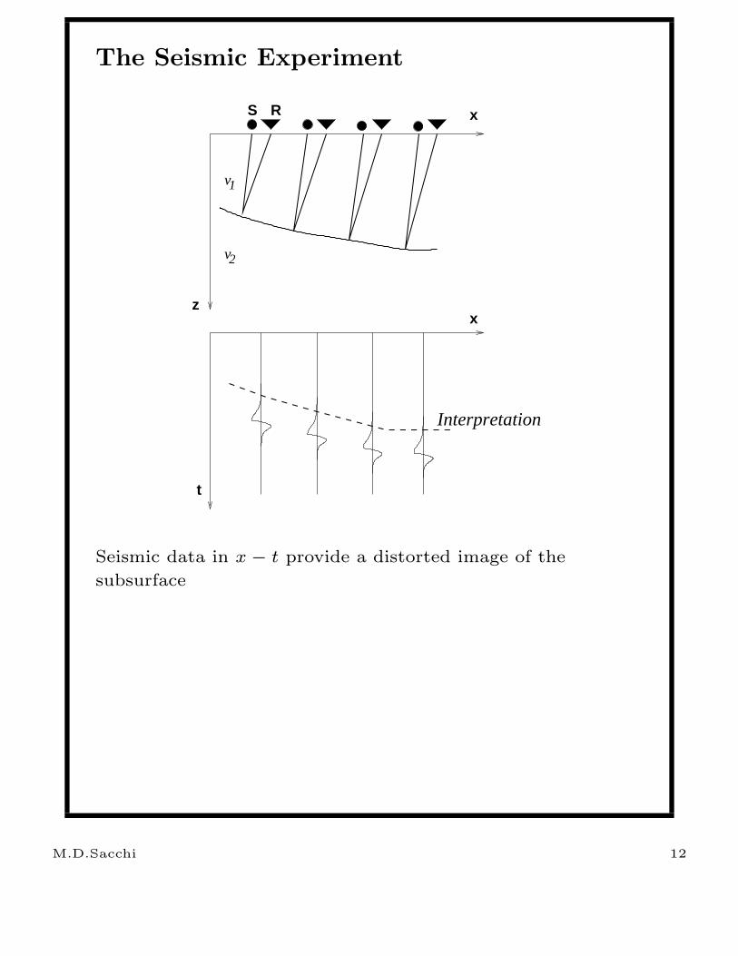
The Seismic Experiment
Interpretation
������������������������
������������������������
1v
2v
x
z
S R
t
x
Seismic data in x − t provide a distorted image of the
subsurface
M.D.Sacchi 12
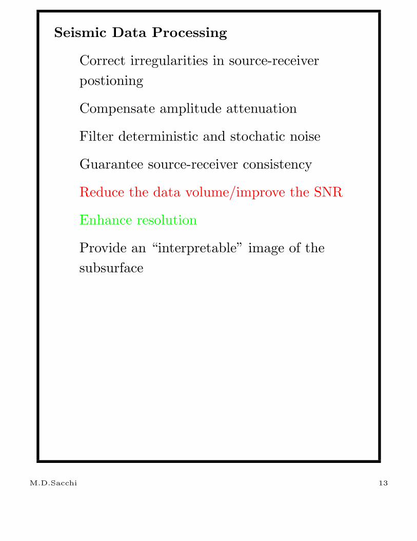
Seismic Data Processing
Correct irregularities in source-receiver
postioning
Compensate amplitude attenuation
Filter deterministic and stochatic noise
Guarantee source-receiver consistency
Reduce the data volume/improve the SNR
Enhance resolution
Provide an “interpretable” image of the
subsurface
M.D.Sacchi 13

Reduce the data volume/improve the SNR
Redundancy in the data is exploited to improve
the SNR
Data(r, s, t) → Image(x, z)
M.D.Sacchi 14
Forward and Inverse Problems
Forward Problem:
Fm = d
F : Mathematical description of the physical
process under study
m: Distribution of physical properties
d: Observations
In the forward problem m and F are given and
we want to compute d at discrete locations.
In general, m(x) is a continuous distribution of
some physical property (velocity is defined
everywhere), whereas d is a discrete vector of
observations di, i = 1 : N
M.D.Sacchi 15

Inverse Problem: Given F and d, we want to
estimate the distribution of physical properties m.
In other words:
1 - Given the data
2 - Given the physical equations
3 - Details about the experiment →What is the distribution of physical properties???
M.D.Sacchi 16
In general, the forward problem can be indicated
as follows:
F : M → D
M : Model Space, a space whose elements consist
of all possible functions or vectors which are
permitted to serve as possible candidates for a
physical model
D: Data Space, a space whose elements consists
of vector of observations d = (d1, d2, d3, . . . , dN )T
Conversely, the inverse problem entails finding the
mapping F−1 such that
F−1 : D → M
M.D.Sacchi 17
Linear and non-linear problems
The function F can be linear or non-linear.
If F is linear the following is true
given m1 ∈ M and m2 ∈ M , then
L(αm1 + βm2) = αLm1 + βLm2
for arbitrary constants α and β. Otherwise is
non-linear.
M.D.Sacchi 18

Fredholm Integral equations of the first
kind
dj =
∫ b
a
gj(x) m(x) dx, j = 1, 2, 3, . . . , N
N : Number of observations
Example: Deconvolution problem
s(tj) =
∫
r(τ)w(tj − τ)dτ
s(tj): observed samples of the seismogram
r(t) : earth’s impulse response (reflectivity)
w(t) : seismic source wavelet
M.D.Sacchi 19

Questions:
Is there a solution ?
How do we construct the solution ?
Is the solution unique ?
Can we characterize the degree
non-uniqueness?
To answer the above questions, we first need to
consider what kind of data we have at hand:
a- Infinite amount of accurate data
b- Finite number of accurate data
c- Finite number of inaccurate data (the real
life scenario!)
M.D.Sacchi 20
Linear Inverse Problems: The Discrete case
We will consider the discrete linear inverse
problem with accurate data. Let us assume that
we have finite amount of data dj , j = 1, . . . N , the
unknown model after discretization using layers
or cells is given by the vector m with elements
mi, i = 1, . . .M . The data as a function of the
model parameters are given by
d = Gm
where G is a N × M matrix that arises after
discretizing the Kernel function of the Forward
problem.
If M > N many solution can solve the above
system of equations.
M.D.Sacchi 21
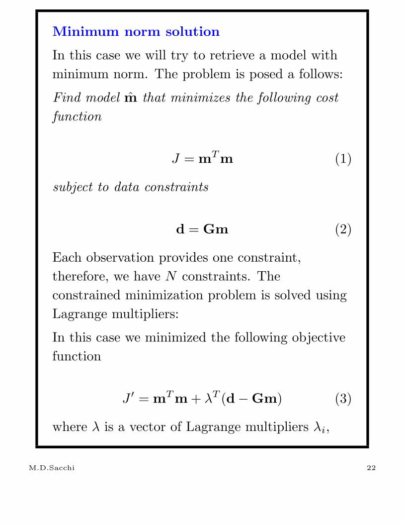
Minimum norm solution
In this case we will try to retrieve a model with
minimum norm. The problem is posed a follows:
Find model m that minimizes the following cost
function
J = mT m (1)
subject to data constraints
d = Gm (2)
Each observation provides one constraint,
therefore, we have N constraints. The
constrained minimization problem is solved using
Lagrange multipliers:
In this case we minimized the following objective
function
J ′ = mT m + λT (d − Gm) (3)
where λ is a vector of Lagrange multipliers λi,
M.D.Sacchi 22
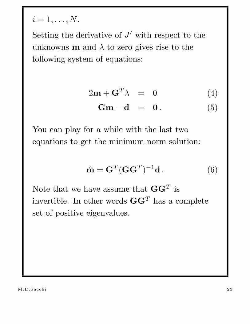
i = 1, . . . , N .
Setting the derivative of J ′ with respect to the
unknowns m and λ to zero gives rise to the
following system of equations:
2m + GT λ = 0 (4)
Gm − d = 0 . (5)
You can play for a while with the last two
equations to get the minimum norm solution:
m = GT (GGT )−1d . (6)
Note that we have assume that GGT is
invertible. In other words GGT has a complete
set of positive eigenvalues.
M.D.Sacchi 23

Example
Suppose that some data dj is the result of the
following experiment
dj = d(rj) =
∫ L
0
e−α(x−rj)2
m(x)dx . (7)
Note that rj can indicate the position of an
observation point (receiver). We can discretize
the above expression using the trapezoidal rule:
d(rj) =
M−1∑
k=0
∆x e−α(rj−xk)2 m(xk) , j = 0 . . . N−1
(8)
Suppose that rj are N observation distributed in
[0, L], then
rj = j . L/(N − 1) , j = 0 . . . N − 1 .
The above system can be written down as
d = Gm (9)
M.D.Sacchi 24
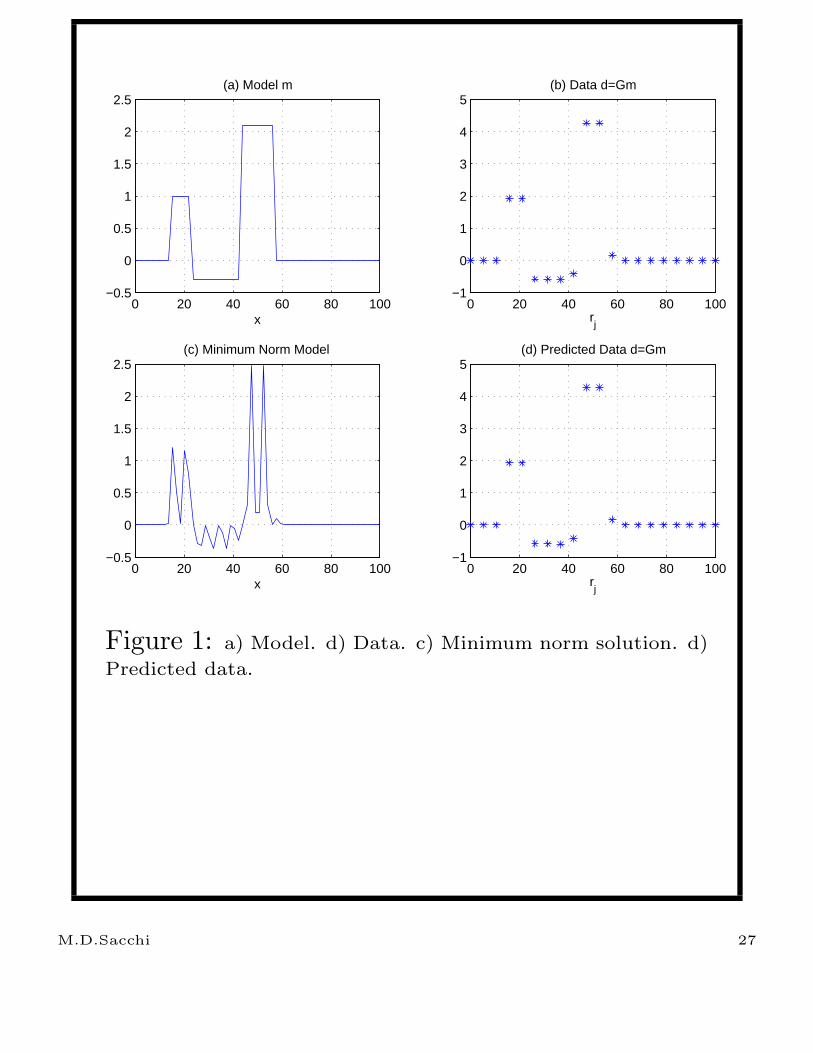
In our example we will assume a true solution
given by the profile m portrayed in Figure 1a.
The corresponding data are displayed in Figure
1b. For this toy problem I have chosen the
following parameters:
α = 0.8, L = 100., N = 20, M = 50
The following script is used to compute the
Kernel G and generate the observations d:
M.D.Sacchi 25
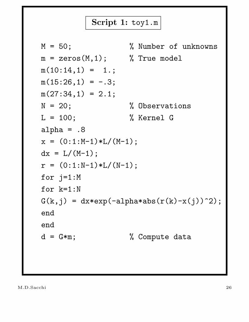
Script 1: toy1.m
M = 50; % Number of unknowns
m = zeros(M,1); % True model
m(10:14,1) = 1.;
m(15:26,1) = -.3;
m(27:34,1) = 2.1;
N = 20; % Observations
L = 100; % Kernel G
alpha = .8
x = (0:1:M-1)*L/(M-1);
dx = L/(M-1);
r = (0:1:N-1)*L/(N-1);
for j=1:M
for k=1:N
G(k,j) = dx*exp(-alpha*abs(r(k)-x(j))^2);
end
end
d = G*m; % Compute data
M.D.Sacchi 26
0 20 40 60 80 100−0.5
0
0.5
1
1.5
2
2.5(a) Model m
x0 20 40 60 80 100
−1
0
1
2
3
4
5(b) Data d=Gm
rj
0 20 40 60 80 100−0.5
0
0.5
1
1.5
2
2.5(c) Minimum Norm Model
x0 20 40 60 80 100
−1
0
1
2
3
4
5(d) Predicted Data d=Gm
rj
Figure 1: a) Model. d) Data. c) Minimum norm solution. d)
Predicted data.
M.D.Sacchi 27
The MATLAB solution for the minimum norm
solution is given by:
Script 2: mns.m
function [m_est,d_pred] = min_norm_sol(G,d);
%
% Given a discrete Kernel G and the data d, computes the
% minimum norm solution of the inverse problem d = Gm.
% m_est: estimates solution (minimum norm solution)
% d_pred: predicted data
m_est = G’*inv(G*G’)*d;
d_pred = G* m_est;
M.D.Sacchi 28

Let’s see how I made Fig.1 using Matlab
Script 3: makefigs.m
% Make figure 1 - 4 figures in the same canvas.
figure(1); clf;
subplot(221);
plot(x,m) ;title(’(a) Model m’); xlabel(’x’);grid;
subplot(222);
plot(r,d,’*’);title(’(b) Data d=Gm’); xlabel(’r_j’);grid
subplot(223);
plot(x,m_est);title(’(c) Minimum Norm Model ’);xlabel(’x’);grid;
subplot(224);
plot(r,d,’*’);title(’(d) Predicted Data d=Gm’); xlabel(’r_j’);grid;
M.D.Sacchi 29

Weighted Minimum norm solution
As we have observed the minimum norm solution
is too oscillatory. To alleviate this problem we
introduce a weighting function into the model
norm. Let us first define a weighted minimum
norm solution
J = ||Wm||2 = mT WT Wm , (10)
this new objective function is minimized subject
to data constraints Gm = d.
m = QGT (GQGT )−1d (11)
where
Q = (WT W)−1 (12)
This solution is called the minimum weighted
norm solution.
M.D.Sacchi 30

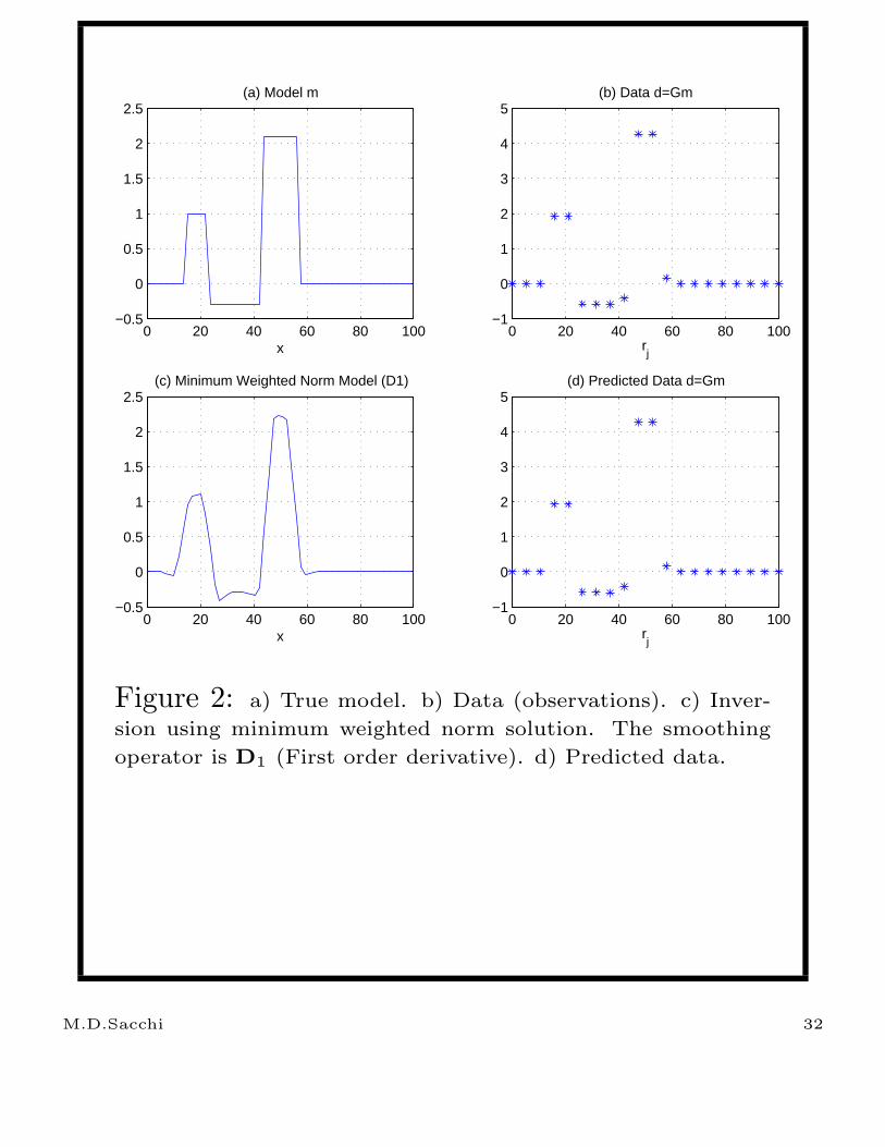
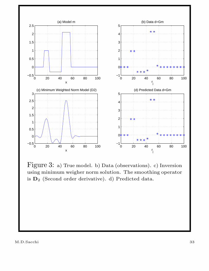
In Figs. 2 and 3, I computed the minimum norm
weighted solution using W = D1 and W = D2,
that is the first derivative operator and the
second derivative operator respectively.
M.D.Sacchi 31
0 20 40 60 80 100−0.5
0
0.5
1
1.5
2
2.5(a) Model m
x0 20 40 60 80 100
−1
0
1
2
3
4
5(b) Data d=Gm
rj
0 20 40 60 80 100−0.5
0
0.5
1
1.5
2
2.5(c) Minimum Weighted Norm Model (D1)
x0 20 40 60 80 100
−1
0
1
2
3
4
5(d) Predicted Data d=Gm
rj
Figure 2: a) True model. b) Data (observations). c) Inver-
sion using minimum weighted norm solution. The smoothing
operator is D1 (First order derivative). d) Predicted data.
M.D.Sacchi 32
0 20 40 60 80 100−0.5
0
0.5
1
1.5
2
2.5(a) Model m
x0 20 40 60 80 100
−1
0
1
2
3
4
5(b) Data d=Gm
rj
0 20 40 60 80 100−0.5
0
0.5
1
1.5
2
2.5
3(c) Minimum Weighted Norm Model (D2)
x0 20 40 60 80 100
−1
0
1
2
3
4
5(d) Predicted Data d=Gm
rj
Figure 3: a) True model. b) Data (observations). c) Inversion
using minimum weigher norm solution. The smoothing operator
is D2 (Second order derivative). d) Predicted data.
M.D.Sacchi 33

This is the MATLAB script that I used to
compute the solution with 1D first order
derivative smoothing:
Script 3: toy1.m
W = convmtx([1,-1],M); % Trick to compute D1
D1 = W(1:M,1:M);
Q = inv(D1’*D1); % Matrix of weights
m_est = Q*G’*inv(G*Q*G’)*d; % Solution
M.D.Sacchi 34

Similarly, you can use second order derivatives:
Script 4: toy1.m
W = convmtx([1,-2,1],M);
D2 = W(1:M,1:M);
Q = inv(D2’*D2);
m_est = Q*G’*inv(G*Q*G’)*d;
M.D.Sacchi 35

The Derivative operators D1 and D2 behave like
high pass filters. If you are not convince compute
the amplitude spectrum of a signal/model after
and before applying one of these operators.
Question: We want to find smooth solutions then,
why are we using High Pass operators?
M.D.Sacchi 36
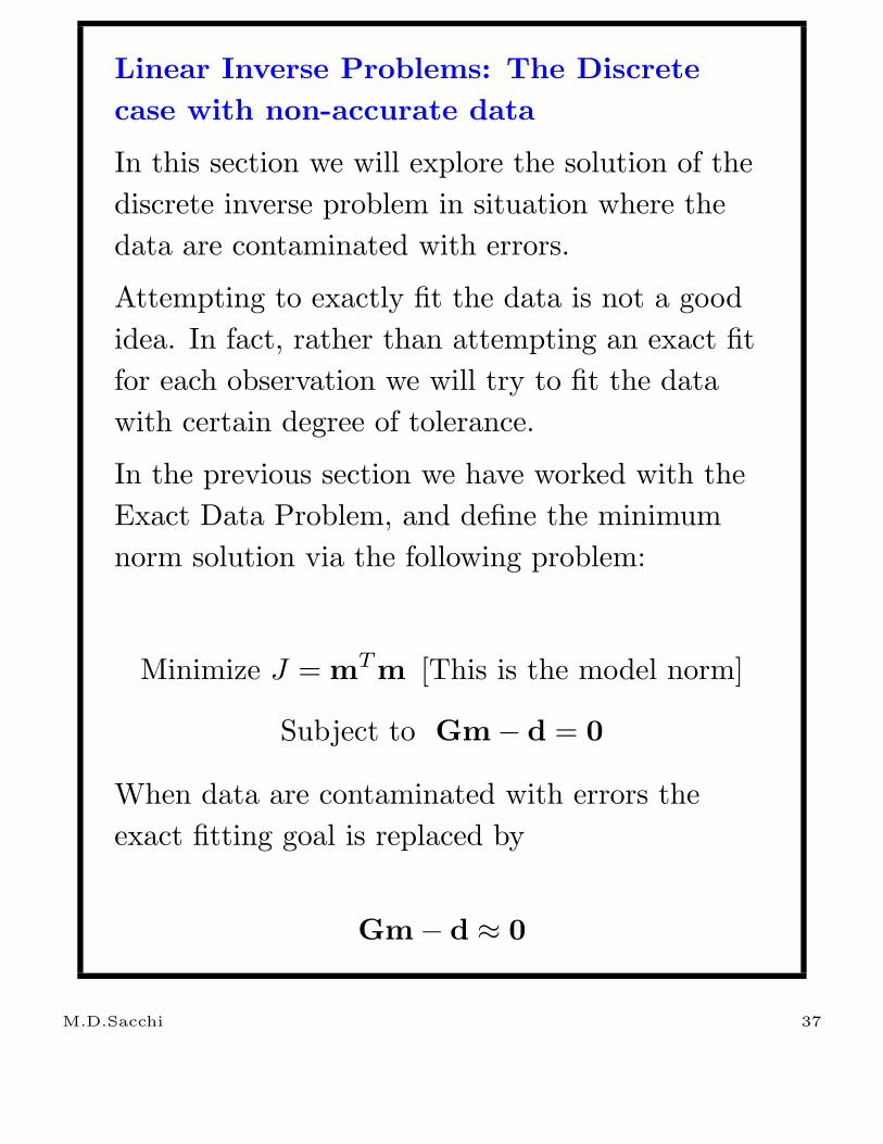
Linear Inverse Problems: The Discrete
case with non-accurate data
In this section we will explore the solution of the
discrete inverse problem in situation where the
data are contaminated with errors.
Attempting to exactly fit the data is not a good
idea. In fact, rather than attempting an exact fit
for each observation we will try to fit the data
with certain degree of tolerance.
In the previous section we have worked with the
Exact Data Problem, and define the minimum
norm solution via the following problem:
Minimize J = mT m [This is the model norm]
Subject to Gm − d = 0
When data are contaminated with errors the
exact fitting goal is replaced by
Gm − d ≈ 0
M.D.Sacchi 37

A model like the above can also be written as
Gm = d + e
where e is used to indicate the error or noise
vector. This quantity is unknown.
M.D.Sacchi 38
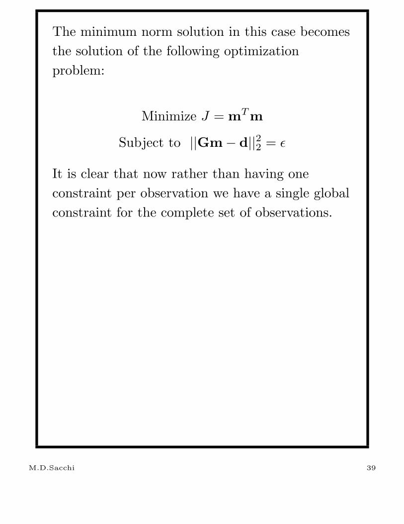
The minimum norm solution in this case becomes
the solution of the following optimization
problem:
Minimize J = mT m
Subject to ||Gm − d||22 = ε
It is clear that now rather than having one
constraint per observation we have a single global
constraint for the complete set of observations.
M.D.Sacchi 39

Please, notice that in the previous equation we
have used the l2 norm as a measure of distance
for the errors in the data; we will see that this
also implies that the errors are considered to be
distributed according to the normal law
(Gaussian errors). Before continuing with the
analysis, we recall that
||Gm − d||22 = ||e||22
which in matrix/vector notation can be also
expressed as
||e||22 = eT e .
Coming back to our optimization problem, we
now minimize the cost function J ′ given by
J ′ = µModel Norm + Misfit
= µmT m + eT e
= µmT m + (Gm − d)T (Gm − d)
M.D.Sacchi 40

The solution is now obtained by minimizing J ′
with respect to the unknown m. This requires
some algebra and I will give you the final solution:
d J ′
dm = 0
= (GT G + µI)m − GT d = 0 .
The minimizer is then given by
m = (GT G + µI)−1GT d . (13)
This solution is often called the damped least
squares solution. Notice that the structure of the
solution looks like the solution we obtain when we
solve a least squares problem. A simple identity
permits one to make equation (13) look like a
minimum norm solution:
M.D.Sacchi 41

Identity (GT G + I)−1GT = GT (GGT + I)−1 .
Therefore, equation (13) can be re-expressed as
m = GT (GGT + µI)−1d . (14)
It is important to note that the previous
expression reduces to the minimum norm solution
for exact data when µ = 0.
M.D.Sacchi 42

About µ
The importance of µ can be seen from the cost
function J ′
J ′ = µModel Norm + Misfit
• Large µ means more weight (importance) is
given to minimizing the misfit over the model
norm.
• Small µ means that the model norm is the
main term entering in the minimization; the
misfit becomes less important.
• You can think that we are trying to
simultaneously achieve two goals:
Norm Reduction (Stability - we don’t
want higly oscillatory solutions)
Misfit Reduction (We want to honor our
observations)
We will explore the fact that these two goals
cannot be simultaneously achieved, and, this is
why we often call µ a trade-off parameter.
M.D.Sacchi 43
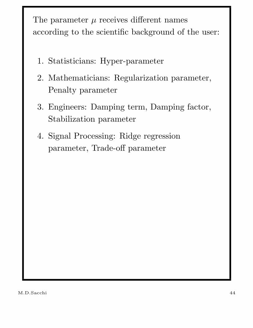
The parameter µ receives different names
according to the scientific background of the user:
1. Statisticians: Hyper-parameter
2. Mathematicians: Regularization parameter,
Penalty parameter
3. Engineers: Damping term, Damping factor,
Stabilization parameter
4. Signal Processing: Ridge regression
parameter, Trade-off parameter
M.D.Sacchi 44

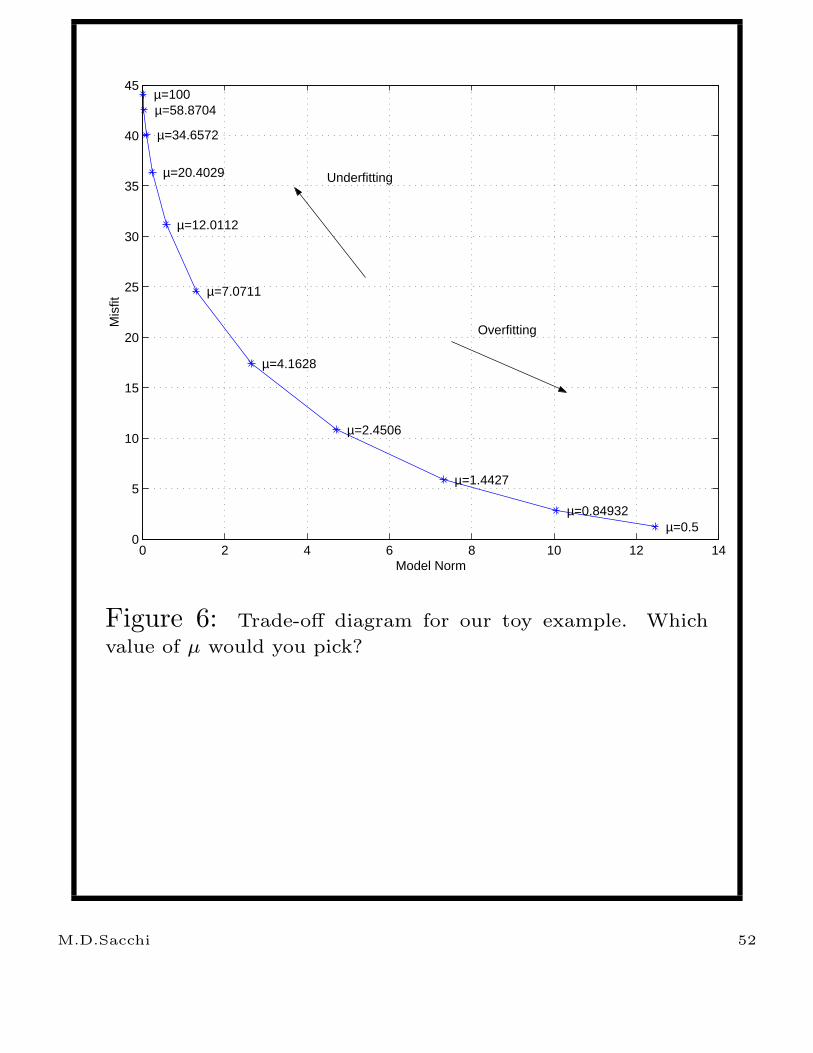
Trade-off diagrams
A trade-off diagram is a display of the model
norm versus the misfit for different values of µ.
Say we have computed a solution for a value µ
this gives the model estimate:
m(µ) = (GT G + µI)−1GT d
This solution can be used to compute the model
norm and the misfit:
Model Norm J(µ) = m(µ)Tm(µ)
Misfit(µ) = (Gm(µ) − d)T (Gm(µ) − d)
by varying µ, we get a curve of J(µ) versus
Misfit(µ).
M.D.Sacchi 45

Example
We use the toy example given by Script 1 to
examine the influence of the trade-off parameter
in the solution of our inverse problem. But first, I
will add noise to the synthetic data generated by
script (toy.m). I basically add a couple of lines to
the code:
Script 5
% Add noise to synthetic data
%
dc = G*m; % Compute clean data
s = 0.1; % Standart error of the noise
d = dc + s*randn(size(dc)); % Add noise
M.D.Sacchi 46

The Least Squares Minimum Norm solution is
obtained with the following script
Script 6
% LS Min Norm Solution
%
I = eye(N);
m_est = G’*((G*G’+mu*I)\d);
Don’t forget our identity; the solution can also be
written in the following form:
Script 6’
% Damped LS Solution
%
I = eye(M);
m_est = (G’*G+mu*I)\ (G’*d);
Q - Script 6 or Script 6’?? Which one would you
use??
M.D.Sacchi 47

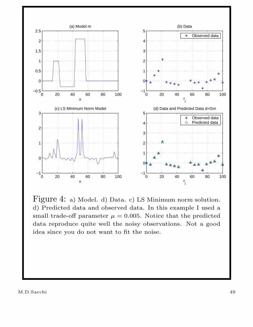
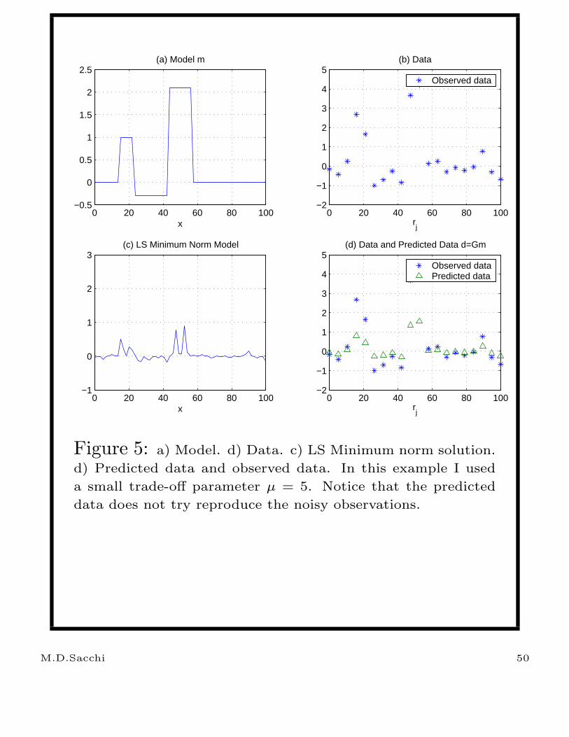
Inversion of the noisy data using the least squares
minimum norm solution for µ = 0.05 and µ = 5.
are portrayed in Figures 4 and 5, respectively.
Notice, that a small value of µ leads to data
over-fitting. In other words, we are attempting to
reproduce the noisy observations like if they were
accurate observations. This is not a good idea
since over-fitting can force the creation of
non-physical features in the solution (highly
oscillatory solutions).
M.D.Sacchi 48
0 20 40 60 80 100−0.5
0
0.5
1
1.5
2
2.5(a) Model m
x0 20 40 60 80 100
−1
0
1
2
3
4
5(b) Data
rj
Observed data
0 20 40 60 80 100−1
0
1
2
3(c) LS Minimum Norm Model
x0 20 40 60 80 100
−1
0
1
2
3
4
5(d) Data and Predicted Data d=Gm
rj
Observed dataPredicted data
Figure 4: a) Model. d) Data. c) LS Minimum norm solution.
d) Predicted data and observed data. In this example I used a
small trade-off parameter µ = 0.005. Notice that the predicted
data reproduce quite well the noisy observations. Not a good
idea since you do not want to fit the noise.
M.D.Sacchi 49
0 20 40 60 80 100−0.5
0
0.5
1
1.5
2
2.5(a) Model m
x0 20 40 60 80 100
−2
−1
0
1
2
3
4
5(b) Data
rj
Observed data
0 20 40 60 80 100−1
0
1
2
3(c) LS Minimum Norm Model
x0 20 40 60 80 100
−2
−1
0
1
2
3
4
5(d) Data and Predicted Data d=Gm
rj
Observed dataPredicted data
Figure 5: a) Model. d) Data. c) LS Minimum norm solution.
d) Predicted data and observed data. In this example I used
a small trade-off parameter µ = 5. Notice that the predicted
data does not try reproduce the noisy observations.
M.D.Sacchi 50
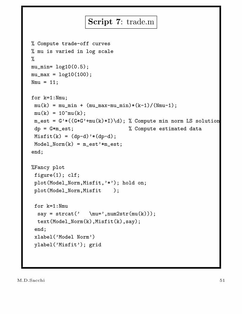
Script 7: trade.m
% Compute trade-off curves
% mu is varied in log scale
%
mu_min= log10(0.5);
mu_max = log10(100);
Nmu = 11;
for k=1:Nmu;
mu(k) = mu_min + (mu_max-mu_min)*(k-1)/(Nmu-1);
mu(k) = 10^mu(k);
m_est = G’*((G*G’+mu(k)*I)\d); % Compute min norm LS solution
dp = G*m_est; % Compute estimated data
Misfit(k) = (dp-d)’*(dp-d);
Model_Norm(k) = m_est’*m_est;
end;
%Fancy plot
figure(1); clf;
plot(Model_Norm,Misfit,’*’); hold on;
plot(Model_Norm,Misfit );
for k=1:Nmu
say = strcat(’ \mu=’,num2str(mu(k)));
text(Model_Norm(k),Misfit(k),say);
end;
xlabel(’Model Norm’)
ylabel(’Misfit’); grid
M.D.Sacchi 51
0 2 4 6 8 10 12 140
5
10
15
20
25
30
35
40
45
µ=0.5 µ=0.84932
µ=1.4427
µ=2.4506
µ=4.1628
µ=7.0711
µ=12.0112
µ=20.4029
µ=34.6572
µ=58.8704 µ=100
Model Norm
Mis
fit
Underfitting
Overfitting
Figure 6: Trade-off diagram for our toy example. Which
value of µ would you pick?
M.D.Sacchi 52

Smoothing in the presence of noise
In this case we minimize:
J ′ = µModel Norm + Misfit
= µ(Wm)T (Wm) + eT e
= µmWT Wm + (Gm − d)T (Gm − d)
where W can be a matrix of first or second order
derivatives as shown before. The minimization of
J ′ leads to a least squares weighted minimum
norm solution
d J ′
dm = 0
= (GT G + µWT W)m − GT d = 0 .
or,
m = (GT G + µWT W)−1GT d
Exercise: Try to rewrite last equation in a way that looks like
a minimum norm solution, this is a solution that contains the
operator GGT .
M.D.Sacchi 53

Script 8: mwnls.m
% Trade-off parameter
%
mu = 5.;
%
% First derivative operator
%
W = convmtx([1,-1],M);
W1 = W(1:M,1:M);
m_est = (G’*G+mu*W1’*W1)\(G’*d);
dp = G*m_est;
Model_Norm = m_est’*m_est;
Misfit = (d-dp)’*(d-dp);
M.D.Sacchi 54

0 20 40 60 80 100−0.5
0
0.5
1
1.5
2
2.5(a) Model m
x0 20 40 60 80 100
−4
−2
0
2
4
6(b) Data
rj
Observed data
0 20 40 60 80 100−1
0
1
2
3(c) LS Minimum Weigthed Norm Model
x0 20 40 60 80 100
−4
−2
0
2
4
6(d) Data and Predicted Data d=Gm
rj
Observed dataPredicted data
Figure 7: a) Model. d) Data. c) LS Minimum Weighted
norm solution. d) Predicted data and observed data. In this
example I used a trade-off parameter µ = 5. Notice that the
predicted data does not try reproduce the noisy observations.
In this example the model norm is ||Wm||22
where W is the
first order derivative operator D1. This example was computed
with Script 8
M.D.Sacchi 55
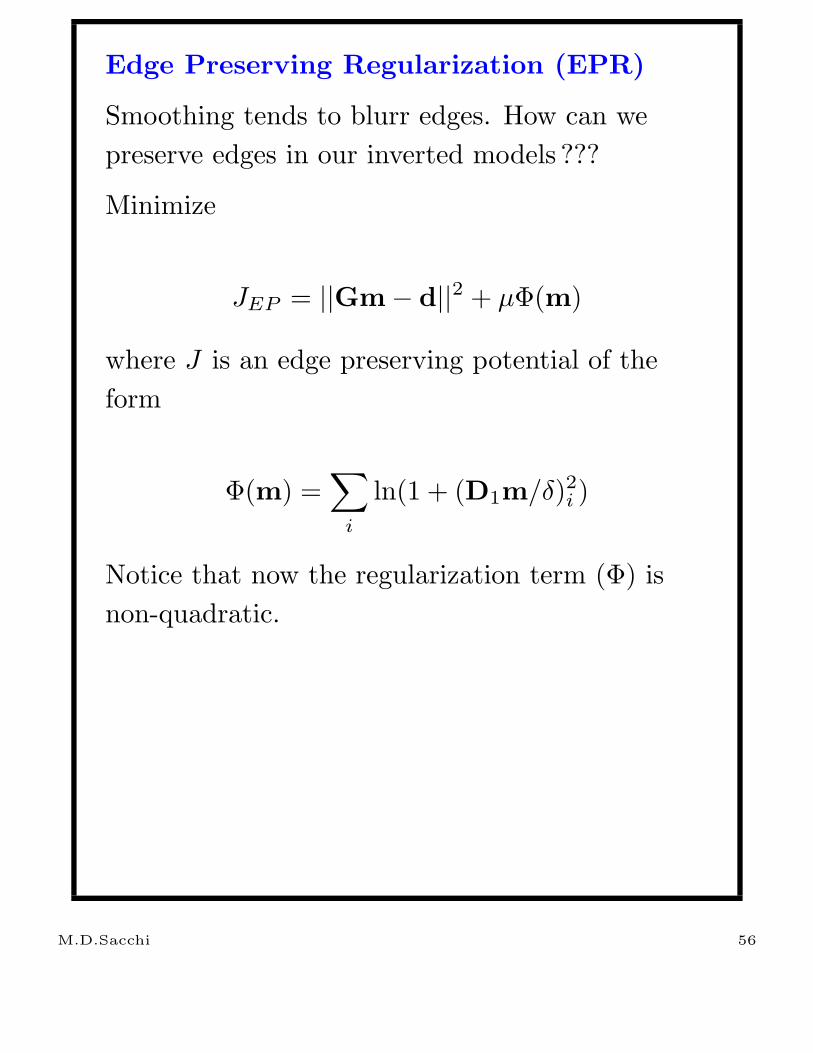
Edge Preserving Regularization (EPR)
Smoothing tends to blurr edges. How can we
preserve edges in our inverted models ???
Minimize
JEP = ||Gm − d||2 + µΦ(m)
where J is an edge preserving potential of the
form
Φ(m) =∑
i
ln(1 + (D1m/δ)2i )
Notice that now the regularization term (Φ) is
non-quadratic.
M.D.Sacchi 56

The EP solution involves an iterative solution of
the following system:
mk = (GT G + µQk−1)−1 GT d
where Q is a diagonal matrix that depends on m.
k indicates iteration number.
M.D.Sacchi 57
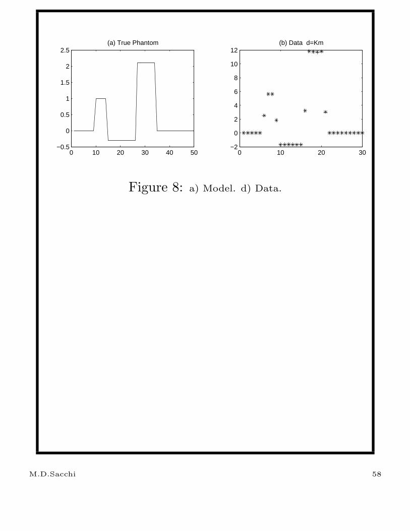
0 10 20 30 40 50−0.5
0
0.5
1
1.5
2
2.5(a) True Phantom
0 10 20 30−2
0
2
4
6
8
10
12(b) Data d=Km
Figure 8: a) Model. d) Data.
M.D.Sacchi 58

0 50 100 150 200−0.5
0
0.5
1
1.5
2
2.5(a) First order Smoothing
0 50 100 150 200−0.5
0
0.5
1
1.5
2
2.5(b) Second order Smoothing
x
0 50 100 150 200−0.5
0
0.5
1
1.5
2
2.5(c) Edge Preserving regularization
Figure 9: a) and b) Smooth solution obtained with quadratic
regularization (first and second order derivative smoothing) c)
Edge preserving solution.
Email me for the EPR scripts: [email protected]
M.D.Sacchi 59
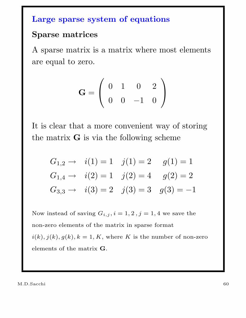
Large sparse system of equations
Sparse matrices
A sparse matrix is a matrix where most elements
are equal to zero.
G =
0 1 0 2
0 0 −1 0
It is clear that a more convenient way of storing
the matrix G is via the following scheme
G1,2 → i(1) = 1 j(1) = 2 g(1) = 1
G1,4 → i(2) = 1 j(2) = 4 g(2) = 2
G3,3 → i(3) = 2 j(3) = 3 g(3) = −1
Now instead of saving Gi,j , i = 1, 2 , j = 1, 4 we save the
non-zero elements of the matrix in sparse format
i(k), j(k), g(k), k = 1, K, where K is the number of non-zero
elements of the matrix G.
M.D.Sacchi 60
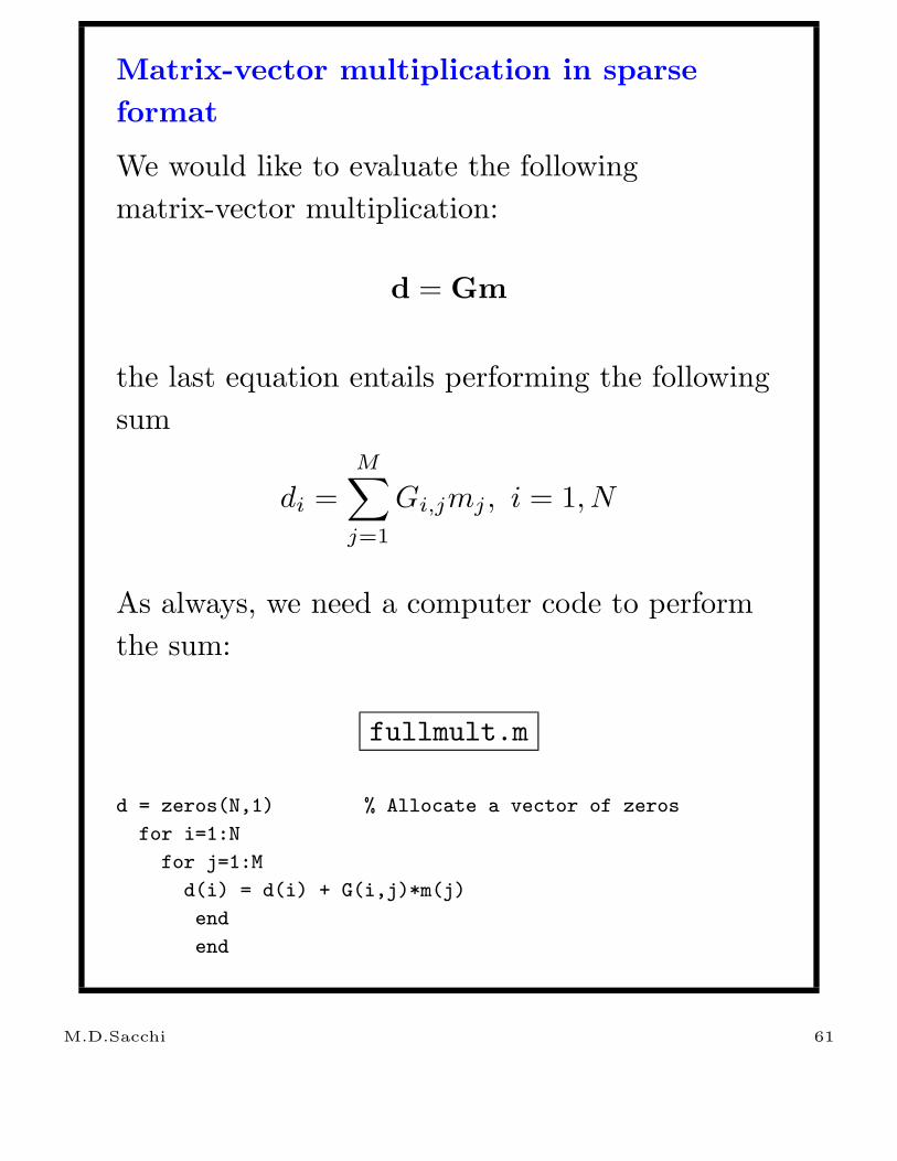
Matrix-vector multiplication in sparse
format
We would like to evaluate the following
matrix-vector multiplication:
d = Gm
the last equation entails performing the following
sum
di =
M∑
j=1
Gi,jmj , i = 1, N
As always, we need a computer code to perform
the sum:
fullmult.m
d = zeros(N,1) % Allocate a vector of zeros
for i=1:N
for j=1:M
d(i) = d(i) + G(i,j)*m(j)
end
end
M.D.Sacchi 61

Let’s see how many operations have been used to
multiple G times m
Number of sums = M*N
Number of products = N*M
M.D.Sacchi 62

If G is sparse and we use the sparse format
storage, the matrix-vector multiplication can be
written as:
sparsemult.m
d = zeros(N,1) % Allocate a vector of zeros
for k=1:K
d(i(k)) = d(i(k)) + g(k)*m(j(k))
end
Now the total number of operations is given by
Number of sums = K
Number of products = K
It is clear that only when sparsity of the matrix
K/(N × M) << 1 there is an important
computational saving.
M.D.Sacchi 63
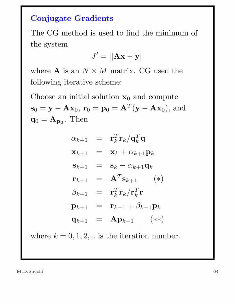
Conjugate Gradients
The CG method is used to find the minimum of
the system
J ′ = ||Ax − y||where A is an N × M matrix. CG used the
following iterative scheme:
Choose an initial solution x0 and compute
s0 = y − Ax0, r0 = p0 = AT (y − Ax0), and
q0 = Ap0. Then
αk+1 = rTk rk/qT
k q
xk+1 = xk + αk+1pk
sk+1 = sk − αk+1qk
rk+1 = AT sk+1 (∗)βk+1 = rT
k rk/rTk r
pk+1 = rk+1 + βk+1pk
qk+1 = Apk+1 (∗∗)
where k = 0, 1, 2, .. is the iteration number.
M.D.Sacchi 64

Theoretically, the minimum is found after M
iterations (steps). In general, we will stop in a
number of iterations M ′ < M an be happy with
an approximate solution. It is clear that all the
computational cost of minimizing J ′ using CG is
in the lines I marked ∗ and ∗∗.
M.D.Sacchi 65
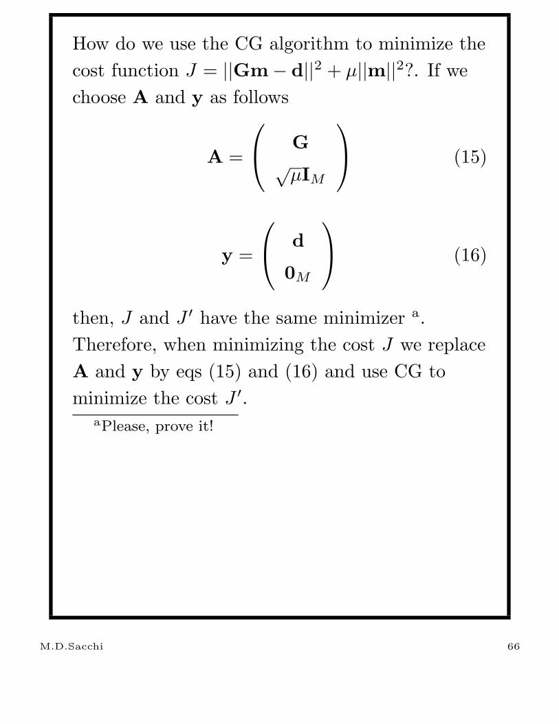
How do we use the CG algorithm to minimize the
cost function J = ||Gm − d||2 + µ||m||2?. If we
choose A and y as follows
A =
G√
µIM
(15)
y =
d
0M
(16)
then, J and J ′ have the same minimizer a.
Therefore, when minimizing the cost J we replace
A and y by eqs (15) and (16) and use CG to
minimize the cost J ′.aPlease, prove it!
M.D.Sacchi 66
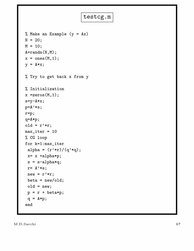
testcg.m
% Make an Example (y = Ax)
N = 20;
M = 10;
A=randn(N,M);
x = ones(M,1);
y = A*x;
% Try to get back x from y
% Initialization
x =zeros(M,1);
s=y-A*x;
p=A’*s;
r=p;
q=A*p;
old = r’*r;
max_iter = 10
% CG loop
for k=1:max_iter
alpha = (r’*r)/(q’*q);
x= x +alpha*p;
s = s-alpha*q;
r= A’*s;
new = r’*r;
beta = new/old;
old = new;
p = r + beta*p;
q = A*p;
end
M.D.Sacchi 67

An excellent tutorial for CG methods:
Jonathan Richard Shewchuk, An Introduction to the
Conjugate Gradient Method Without the Agonizing Pain,
1994. [http://www-2.cs.cmu.edu/~ jrs/jrspapers.html]
M.D.Sacchi 68

Imaging vs. inversion
Imaging - Where?
Inversion - Where and What ?
M.D.Sacchi 69
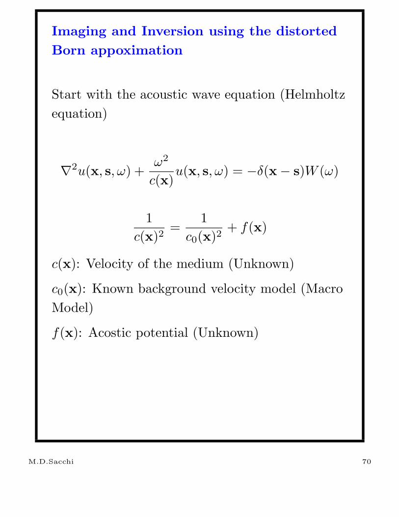
Imaging and Inversion using the distorted
Born appoximation
Start with the acoustic wave equation (Helmholtz
equation)
∇2u(x, s, ω) +ω2
c(x)u(x, s, ω) = −δ(x − s)W (ω)
1
c(x)2=
1
c0(x)2+ f(x)
c(x): Velocity of the medium (Unknown)
c0(x): Known background velocity model (Macro
Model)
f(x): Acostic potential (Unknown)
M.D.Sacchi 70
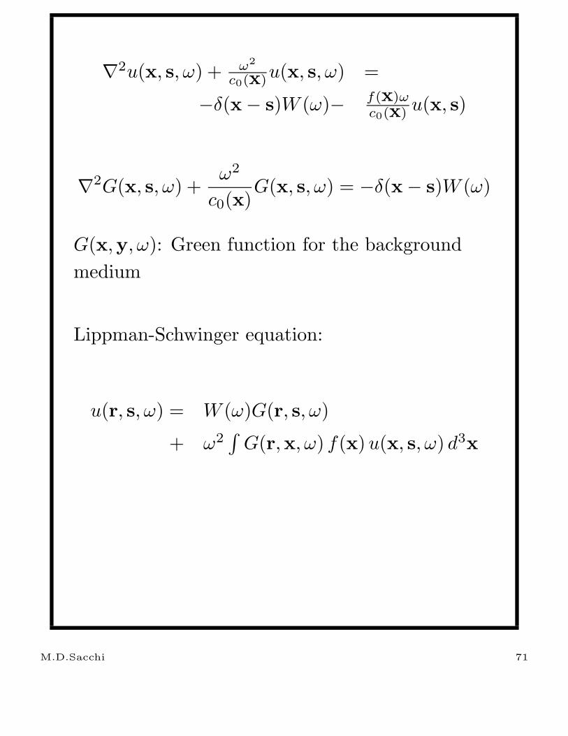
∇2u(x, s, ω) + ω2
c0(x)u(x, s, ω) =
−δ(x − s)W (ω)− f(x)ωc0(x) u(x, s)
∇2G(x, s, ω) +ω2
c0(x)G(x, s, ω) = −δ(x − s)W (ω)
G(x,y, ω): Green function for the background
medium
Lippman-Schwinger equation:
u(r, s, ω) = W (ω)G(r, s, ω)
+ ω2∫
G(r,x, ω) f(x) u(x, s, ω) d3x
M.D.Sacchi 71

u(r, s, ω) = W (ω)G(r, s, ω)
+ ω2∫
G(r,x, ω) f(x) u(x, s, ω) d3x
u(r, s, ω) = uinc(r, s, ω) + usc(r, s, ω)
If usc(r, s, ω) ≈ uinc(r, s, ω) = W (ω)G(r, s, ω)
→Single scattering approximation about the
background medium
usc(r, s, ω) =
ω2W (ω)∫
G(r,x, ω) f(x) G(x, s, ω) d3x
or, in compact notation:
u = Bf
M.D.Sacchi 72

• c0 = constant - First Born Approximation
• c0 = c0(x) - Distorted Born Approximation
• Validity of the approximation requires
c(x) ≈ c0(x)
• G(x,y, ω) can be written explicitly only for
very simple models
• In arbirtrary backgrounds we can use the
First Order Asymtotic approximation
(Geometrical Optics)
G(x,y, ω) = A(x,y)eiω τ(x,y)
M.D.Sacchi 73
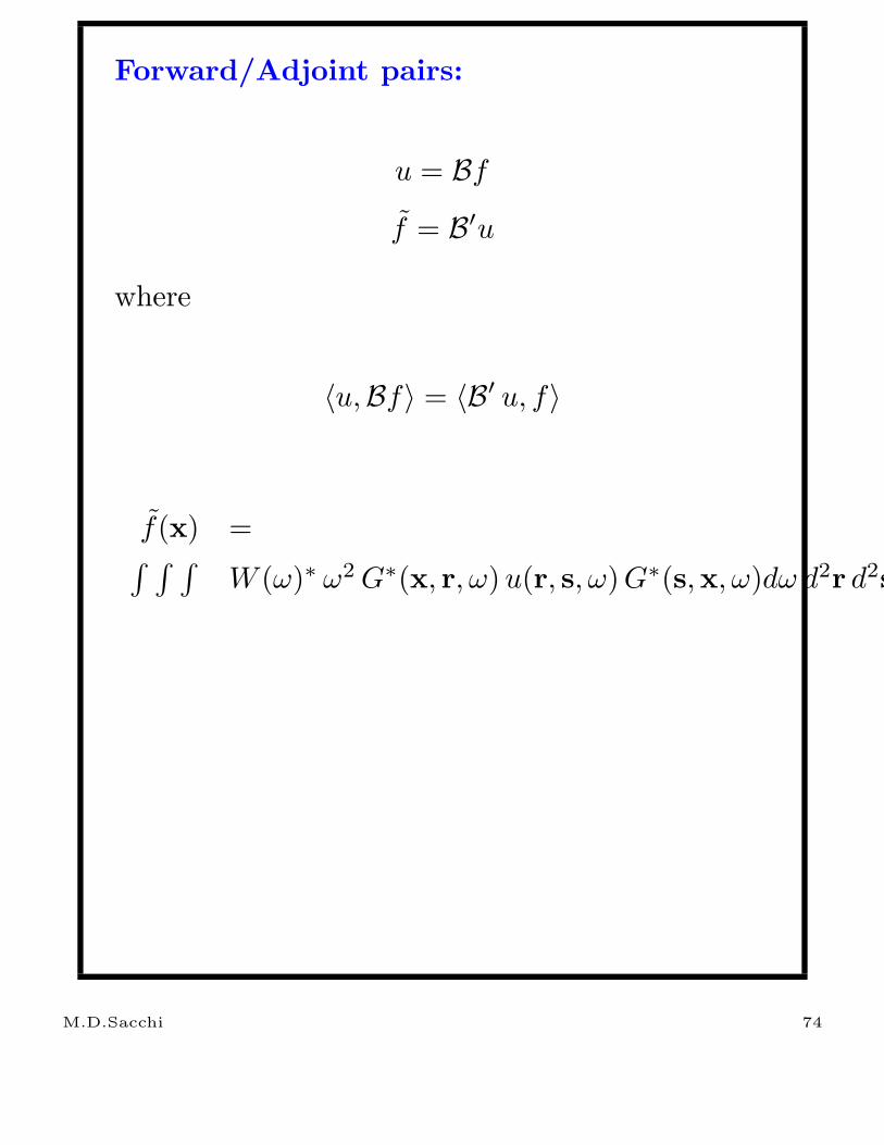
Forward/Adjoint pairs:
u = Bf
f = B′u
where
〈u,Bf〉 = 〈B′ u, f〉
f(x) =∫ ∫ ∫
W (ω)∗ ω2 G∗(x, r, ω) u(r, s, ω) G∗(s,x, ω)dω d2r d2s
M.D.Sacchi 74
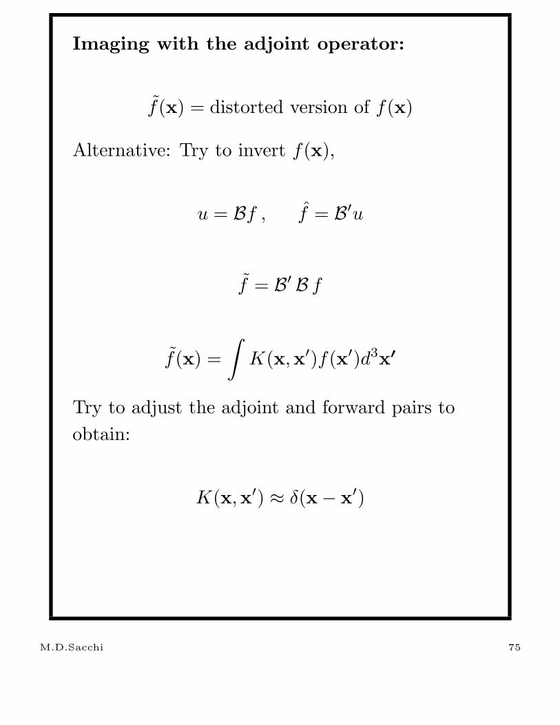
Imaging with the adjoint operator:
f(x) = distorted version of f(x)
Alternative: Try to invert f(x),
u = Bf , f = B′u
f = B′ B f
f(x) =
∫
K(x,x′)f(x′)d3x′
Try to adjust the adjoint and forward pairs to
obtain:
K(x,x′) ≈ δ(x − x′)
M.D.Sacchi 75
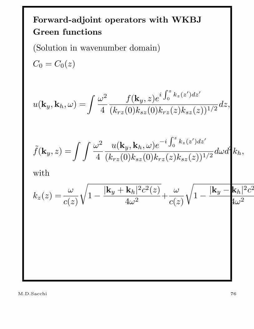
Forward-adjoint operators with WKBJ
Green functions
(Solution in wavenumber domain)
C0 = C0(z)
u(ky,kh, ω) =
∫
ω2
4
f(ky, z)ei∫
z
0kz(z′)dz′
(krz(0)ksz(0)krz(z)ksz(z))1/2dz,
f(ky, z) =
∫ ∫
ω2
4
u(ky,kh, ω)e−i
∫
z
0kz(z′)dz′
(krz(0)ksz(0)krz(z)ksz(z))1/2dωd2kh,
with
kz(z) =ω
c(z)
√
1 − |ky + kh|2c2(z)
4ω2+
ω
c(z)
√
1 − |ky − kh|2c2(z)
4ω2.
M.D.Sacchi 76

Recursive implementation (Downward
continuation)
u(ky,kh, z, ω) = u(ky,kh, ω)e−i
∫
z
0kz(z′)dz′
≈ u(ky,kh, ω)e−i∑
z
z′=0kz(z′)∆z
u(ky,kh, z + ∆z, ω) = u(ky,kh, z, ω)e−ikz(z)∆z
M.D.Sacchi 77

Lateral variant background velocity c0 = c0(x, z)
(Splittinga)
e−ikz(x,z)∆z ≈ e−ikz(z)∆z × e−iω∆S∆z
∆S =2
c0(z)− 1
c0(y + h, z)− 1
c0(y − h, z)
c0(z): mean velocity at depth z
c0(x, z): background velocity
The algorithm recursively downward
continues the data with c0(z) in kh, ky
The split-step correction is applied in y ,h.
aFeit and Fleck’78, Light Propagation in graded-index
fibers, Appl. Opt. 17
M.D.Sacchi 78
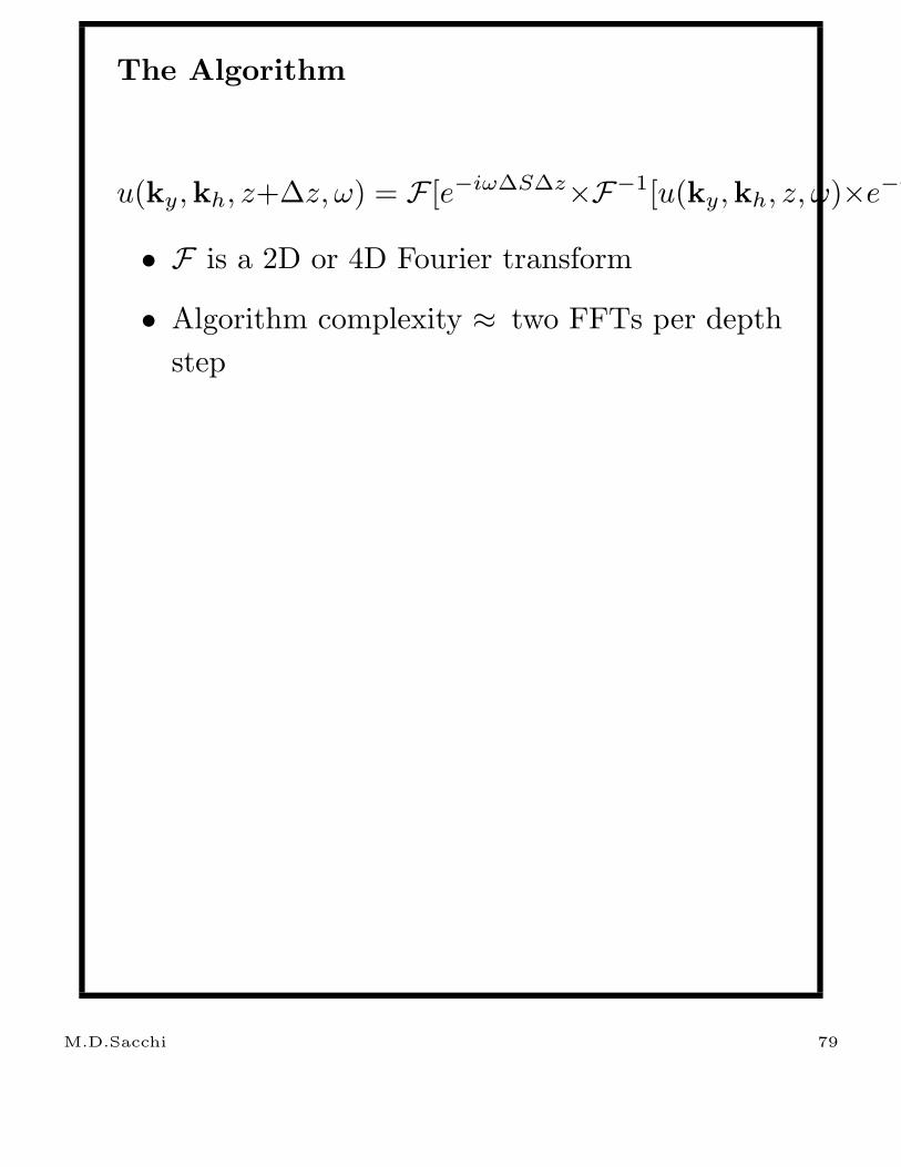
The Algorithm
u(ky,kh, z+∆z, ω) = F [e−iω∆S∆z×F−1[u(ky,kh, z, ω)×e−ikz(z)∆z]]
• F is a 2D or 4D Fourier transform
• Algorithm complexity ≈ two FFTs per depth
step
M.D.Sacchi 79
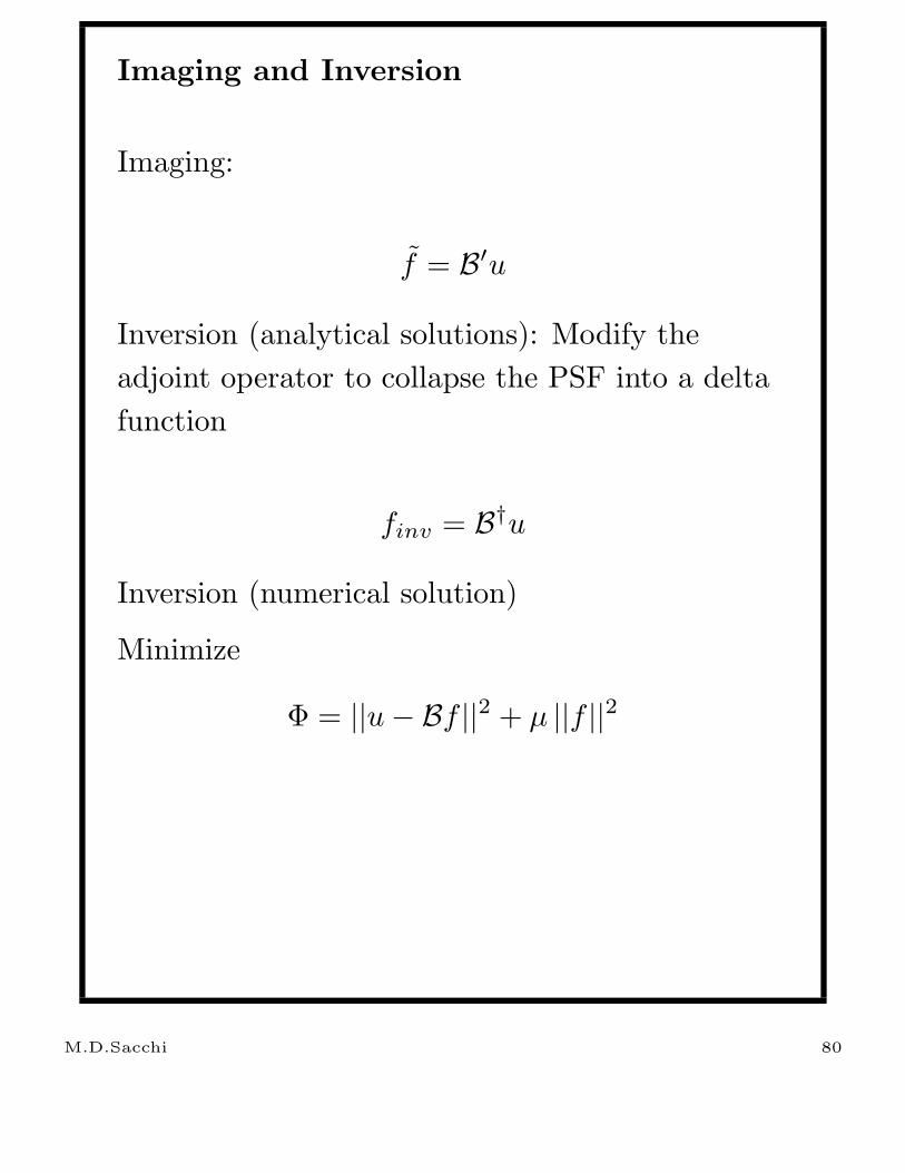
Imaging and Inversion
Imaging:
f = B′u
Inversion (analytical solutions): Modify the
adjoint operator to collapse the PSF into a delta
function
finv = B†u
Inversion (numerical solution)
Minimize
Φ = ||u − Bf ||2 + µ ||f ||2
M.D.Sacchi 80

Inversion (numerical solution) - CG
Method
• CG: Conjugate Gradients to solve large linear
systems of equation (in this case linear
operators)
• Easy to implement if you have B and B′
• Don’t need to iterate forever
M.D.Sacchi 81
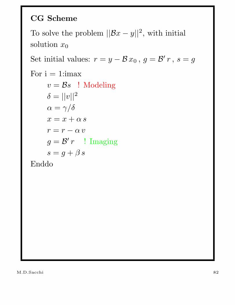
CG Scheme
To solve the problem ||Bx − y||2, with initial
solution x0
Set initial values: r = y − B x0 , g = B′ r , s = g
For i = 1:imax
v = Bs ! Modeling
δ = ||v||2α = γ/δ
x = x + α s
r = r − α v
g = B′ r ! Imaging
s = g + β s
Enddo
M.D.Sacchi 82
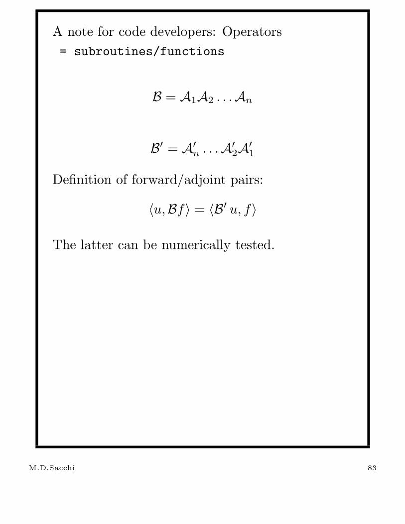
A note for code developers: Operators
= subroutines/functions
B = A1A2 . . .An
B′ = A′n . . .A′
2A′1
Definition of forward/adjoint pairs:
〈u,Bf〉 = 〈B′ u, f〉
The latter can be numerically tested.
M.D.Sacchi 83
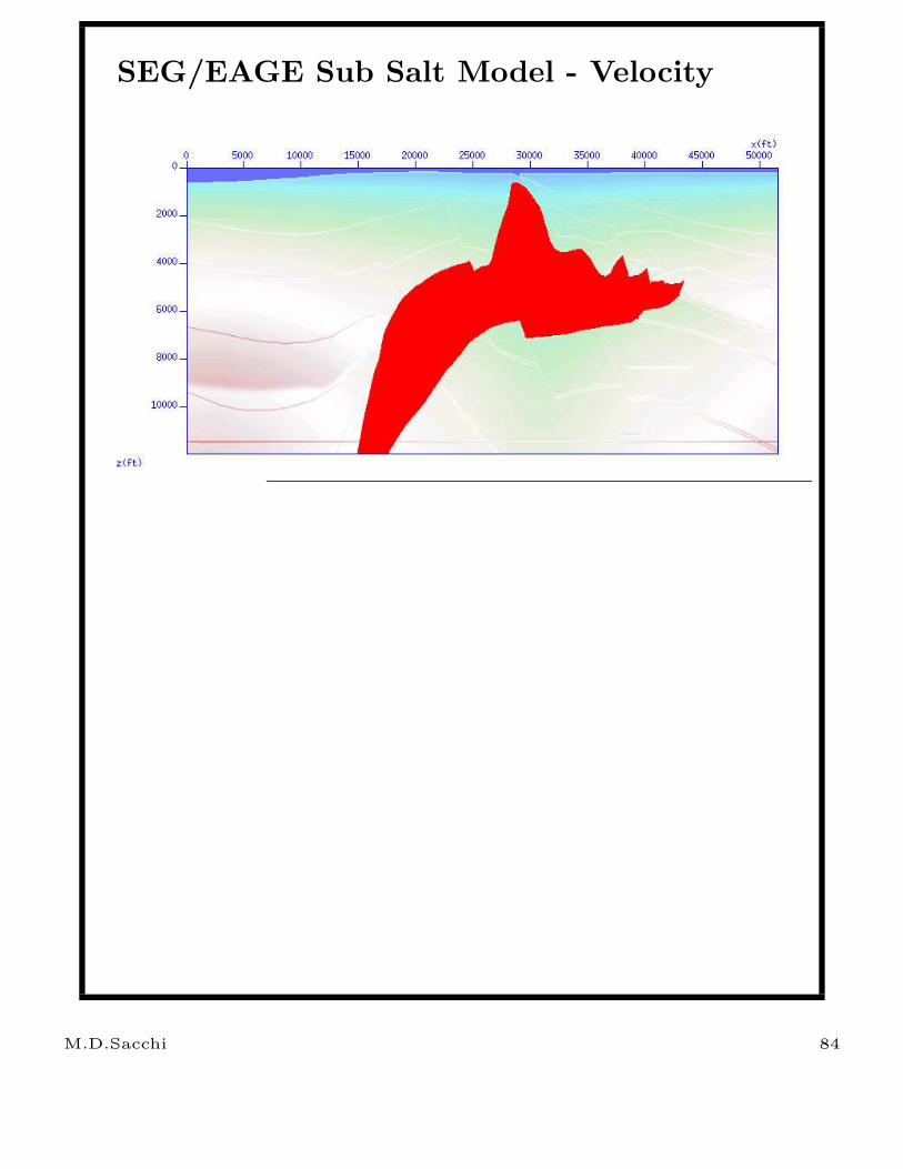
SEG/EAGE Sub Salt Model - Velocity
M.D.Sacchi 84
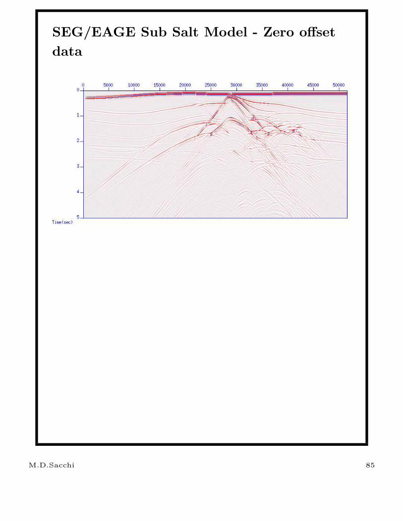
SEG/EAGE Sub Salt Model - Zero offset
data
M.D.Sacchi 85
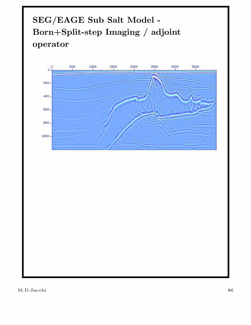
SEG/EAGE Sub Salt Model -
Born+Split-step Imaging / adjoint
operator
M.D.Sacchi 86

Edge Preserving Regularization
J = ||usc−Bf ||2+βx
∑
k
R[(Dxf)k]+βz
∑
k
R[(Dzf)k] .
R(x) = ln(1 + x2)
with spatial derivative operators:
(Dxf)i,j = (fi,j+1 − fi,j)/δx
(Dzf)i,j = (fi+1,1 − fi,j)/δz
M.D.Sacchi 87
1900
2000
2100
2200
2300
2400
2500
Offset (m)
Dep
th (
m)
(A)
0 50 100 150 200
0
50
100
150
200
Offset (m)
Tim
e (s
)
(B)
0 50 100 150
0
0.05
0.1
0.15
1900
2000
2100
2200
2300
2400
2500
Offset (m)
Dep
th (
m)
(C)
0 50 100 150 200
0
50
100
150
200 1900
2000
2100
2200
2300
2400
2500
Offset (m)
Dep
th (
m)
(D)
0 50 100 150 200
0
50
100
150
200
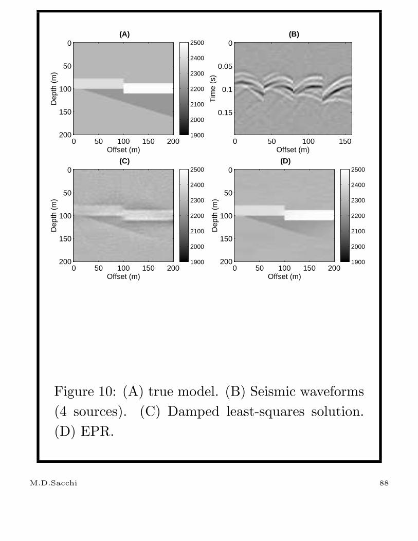
Figure 10: (A) true model. (B) Seismic waveforms
(4 sources). (C) Damped least-squares solution.
(D) EPR.
M.D.Sacchi 88

From Inverse Filters toFrom Inverse Filters to LS LS MigrationMigration
Mauricio Sacchi
Institute for Geophysical Research & Department of Physics
University of Alberta, Edmonton, AB, Canada
Review 1
• Impulse response (hitting the system with an impulse)
y(t) = ∫ h(t −τ )x(τ )dτ = h(t) * x(t)
h(t)
x(t) = δ (t)
x(t) y(t)
h(t)h(t)
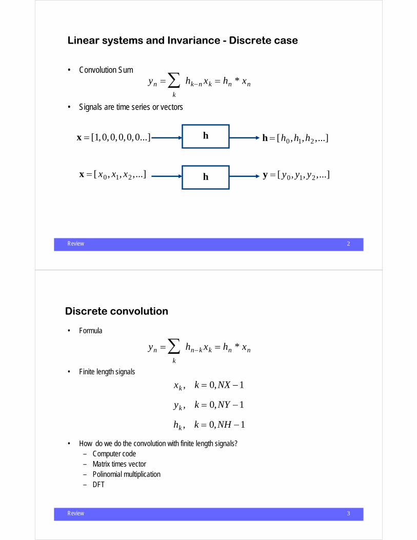
Linear systems and Invariance
Input Inputh(t)δ (t)
Review 2
• Convolution Sum
• Signals are time series or vectors
yn =k
∑ hk−n xk = hn * xn
x = [1,0,0,0,0,0...]
Linear systems and Invariance - Discrete case
h = [h0,h1,h2,...]
x = [ x0, x1, x2,...] y = [ y0, y1, y2,...]
h
h
Review 3
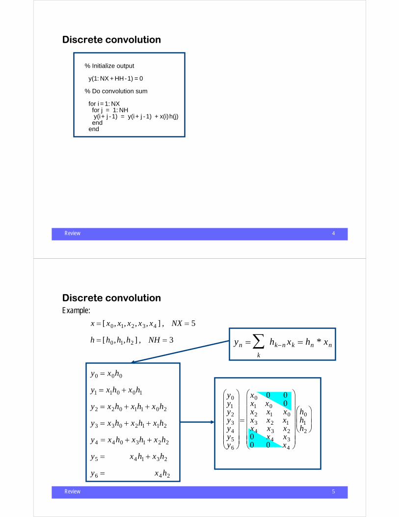
Discrete convolution
• Formula
• Finite length signals
• How do we do the convolution with finite length signals?– Computer code– Matrix times vector– Polinomial multiplication– DFT
yn =k
∑ hn−k xk = hn * xn
xk , k = 0,NX −1
yk , k = 0,NY −1
hk , k = 0,NH −1
Review 4
Discrete convolution
% Initialize output
y(1: NX + HH-1) = 0
% Do convolution sum for i = 1: NX for j = 1: NH y(i+ j -1) = y(i+ j -1) + x(i)h(j) end end
Review 5
Discrete convolution
x = [ x0, x1, x2, x3, x4 ] , NX = 5
h = [h0,h1,h2 ] , NH = 3
y0 = x0h0
y1 = x1h0 + x0h1
y2 = x2h0 + x1h1 + x0h2
y3 = x3h0 + x2h1 + x1h2
y4 = x4h0 + x3h1 + x2h2
y5 = x4h1 + x3h2
y6 = x4h2
yn =k
∑ hk−n xk = hn * xn
Example:
y0y1y2y3y4y5y6
⎛
⎝
⎜ ⎜ ⎜ ⎜ ⎜ ⎜
⎞
⎠
⎟ ⎟ ⎟ ⎟ ⎟ ⎟
=
x0 0 0x1 x0 0x2 x1 x0x3 x2 x1x4 x3 x20 x4 x30 0 x4
⎛
⎝
⎜ ⎜ ⎜ ⎜ ⎜ ⎜
⎞
⎠
⎟ ⎟ ⎟ ⎟ ⎟ ⎟
h0h1h2
⎛
⎝ ⎜ ⎜
⎞
⎠ ⎟ ⎟
Review 6
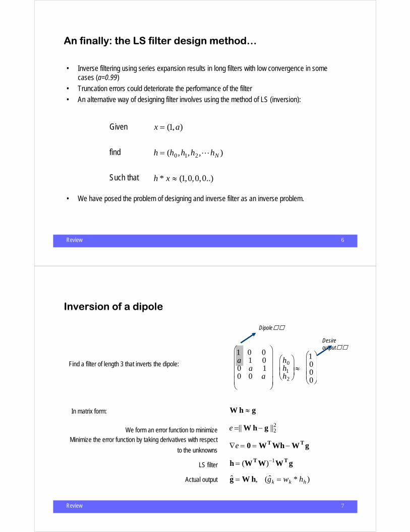
An finally: the LS filter design method…
• Inverse filtering using series expansion results in long filters with low convergence in some cases (a=0.99)
• Truncation errors could deteriorate the performance of the filter
• An alternative way of designing filter involves using the method of LS (inversion):
• We have posed the problem of designing and inverse filter as an inverse problem.
x = (1,a)
h = (h0,h1,h2, hN )
h * x ≈ (1,0,0,0..)
Given
find
Such that
Review 7
1 0 0a 1 00 a 10 0 a
⎛
⎝
⎜ ⎜ ⎜ ⎜
⎞
⎠
⎟ ⎟ ⎟ ⎟
h0h1h2
⎛
⎝ ⎜ ⎜
⎞
⎠ ⎟ ⎟ ≈
1000
⎛
⎝
⎜ ⎜ ⎜
⎞
⎠
⎟ ⎟ ⎟
W h ≈ g
e =|| W h − g ||22
∇e = 0 = WT Wh − WT g
h = (WT W)−1WT g
ˆ g = W h, ( ˆ g k = wk * hh )
Inversion of a dipole
Find a filter of length 3 that inverts the dipole:
In matrix form:
We form an error function to minimizeMinimize the error function by taking derivatives with respect
to the unknowns
LS filter
Actual output
Dipole
Desire output
Review 8
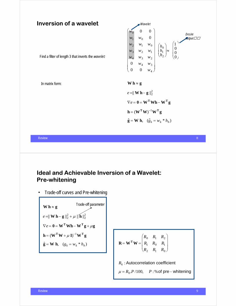
Inversion of a waveletw0 0 0
w1 w0 0
w2 w1 w0
w3 w2 w1
w4 w3 w2
0 w4 w3
0 0 w4
⎛
⎝
⎜ ⎜ ⎜ ⎜ ⎜ ⎜ ⎜ ⎜ ⎜
⎞
⎠
⎟ ⎟ ⎟ ⎟ ⎟ ⎟ ⎟ ⎟ ⎟
h0h1h2
⎛
⎝ ⎜ ⎜
⎞
⎠ ⎟ ⎟ ≈
1000
⎛
⎝
⎜ ⎜ ⎜
⎞
⎠
⎟ ⎟ ⎟
W h ≈ g
e =|| W h − g ||22
∇e = 0 = WT Wh − WT g
h = (WT W)−1WT g
ˆ g = W h, ( ˆ g k = wk * hh )
Find a filter of length 3 that inverts the wavelet:
In matrix form:
Wavelet
Desire output
Review 9
Ideal and Achievable Inversion of a Wavelet:Pre-whitening
• Trade-off curves and Pre-whitening
W h ≈ g
e =|| W h − g ||22 + µ || h ||2
2
∇e = 0 = WT Wh − WT g + µg
h = (WT W + µ I)−1WT g
ˆ g = W h, (gk = wk * hh )
Trade-off parameter
R = WT W =R0 R1 R2
R1 R0 R1
R2 R1 R0
⎛
⎝
⎜ ⎜ ⎜
⎞
⎠
⎟ ⎟ ⎟
Rk : Autocorrelation coefficient
µ = R0.P /100, P :%of pre − whitening
Review 10
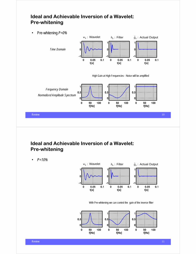
Ideal and Achievable Inversion of a Wavelet:Pre-whitening
• Pre-whitening P=0%
Time Domain
Frequency Domain
Normalized Amplitude Spectrum
wk : Wavelet hk : Filter g k : Actual Output
High Gain at High Frequencies - Noise will be amplified
Review 11
Ideal and Achievable Inversion of a Wavelet:Pre-whitening
• P=10% wk : Wavelet hk : Filter g k : Actual Output
With Pre-whitening we can control the gain of the inverse filter

Review 12
Ideal and Achievable Inversion of a Wavelet:Pre-whitening
• P=20% wk : Wavelet hk : Filter g k : Actual Output
With Pre-whitening we can control the gain of the inverse filter
Review 13
Ideal and Achievable Inversion of a Wavelet:Pre-whitening & Trade-off curve
e =|| W h − g ||22 + µ || h ||2
2
= Misfit + µ Model Norm
Misfit
Model Norm
µ = 0.01µ = 0.1
µ = 1.*
* *
Resolution +Stability -
Resolution -Stability +
Review 14
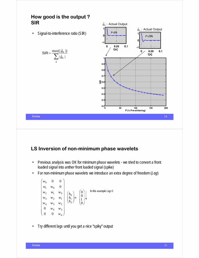
How good is the output ?SIR
• Signal-to-interference ratio (SIR)
SIR =max(| ˆ g k |)
| ˆ g k |k
∑
g k : Actual Output g k : Actual Output
P=0%P=20%
Review 15
LS Inversion of non-minimum phase wavelets
• Previous analysis was OK for minimum phase wavelets - we tried to convert a front loaded signal into anther front loaded signal (spike)
• For non-minimum phase wavelets we introduce an extra degree of freedom (Lag)
• Try different lags until you get a nice “spiky” output
w0 0 0
w1 w0 0
w2 w1 w0
w3 w2 w1
w4 w3 w2
0 w4 w3
0 0 w4
⎛
⎝
⎜ ⎜ ⎜ ⎜ ⎜ ⎜ ⎜ ⎜ ⎜
⎞
⎠
⎟ ⎟ ⎟ ⎟ ⎟ ⎟ ⎟ ⎟ ⎟
h0h1h2
⎛
⎝ ⎜ ⎜
⎞
⎠ ⎟ ⎟ ≈
0010
⎛
⎝
⎜ ⎜ ⎜
⎞
⎠
⎟ ⎟ ⎟
In this example Lag=3
Review 16
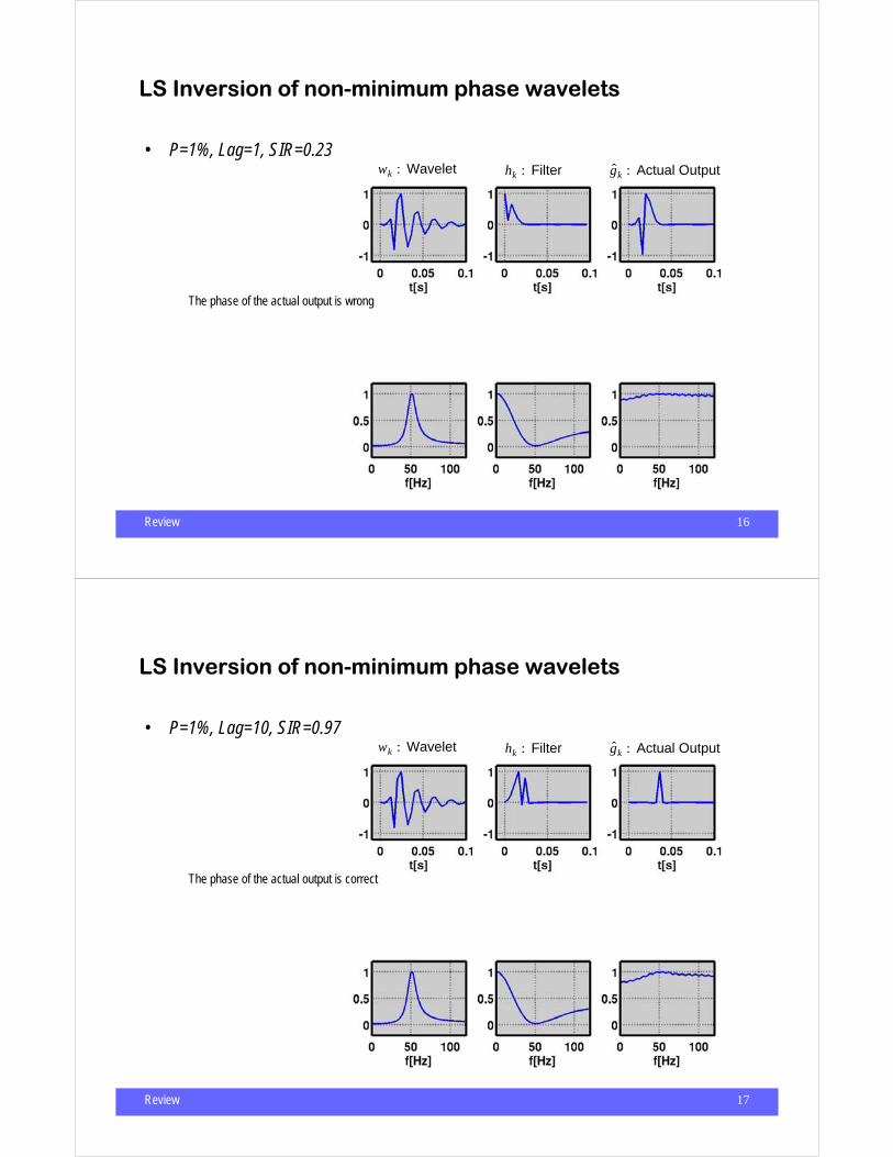
LS Inversion of non-minimum phase wavelets
• P=1%, Lag=1, SIR=0.23 wk : Wavelet hk : Filter g k : Actual Output
The phase of the actual output is wrong
Review 17
LS Inversion of non-minimum phase wavelets
• P=1%, Lag=10, SIR=0.97 wk : Wavelet hk : Filter g k : Actual Output
The phase of the actual output is correct
Review 18
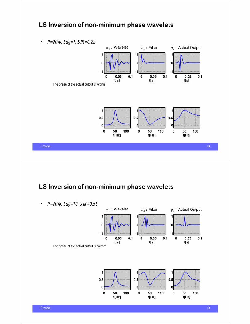
LS Inversion of non-minimum phase wavelets
• P=20%, Lag=1, SIR=0.22 wk : Wavelet hk : Filter g k : Actual Output
The phase of the actual output is wrong
Review 19
LS Inversion of non-minimum phase wavelets
• P=20%, Lag=10, SIR=0.56 wk : Wavelet hk : Filter g k : Actual Output
The phase of the actual output is correct

Review 20
Where does the wavelet come from?
R = WT W =R0 R1 R2
R1 R0 R1
R2 R1 R0
⎛
⎝
⎜ ⎜ ⎜
⎞
⎠
⎟ ⎟ ⎟
• Observations
• Finding the inverse filter requires the matrix R. This is the autocorrelation matrix of the wavelet.
• If the reflectivity is assumed to be white then the autocorrelation of the trace is equal (within a scale factor) to the autocorrelation of the wavelet
• In Short: Since you cannot measure the wavelet or its autocorrelation, we replace the autocorrelation coefficients of the wavelet by those of the trace and then, we hope that the validity of thewhite reflectivity assumption holds!!
RTrace = c RWavelet
Review 21
Why is that ?
Rks = st +ksk
t∑
sk = wk * rk
Rks = Rk
r * Rkw
Rkr = c if k = 0
0 every where else⎧ ⎨ ⎩
Rks = cRk
w
Autocorrelation of the trace s
Convolution model
We can show this one
If reflectivity is white (Geology does not have
memory?)
Then……

Review 22
Color ?
Rks = st +ksk
t∑
sk = wk * rk
Rks = Rk
r * Rkw
Rkw = (Rk
r )−1 * Rks
Autocorrelation of the trace s
Convolution model
We can show this one
If the reflectivity is non-white (Geology does
have memory)
Rosa, A. L. R., and T. J. Ulrych, 1991, Processing via spectral modeling: Geophysics, 56, 1244-1251.
Haffner, S., and S. Cheadle, 1999, Colored reflectivity compensation for increased vertical resolution: 69th Annual International Meeting, SEG, Expanded Abstracts, 1307-1310.
Saggaf, M.M., and E. A. Robinson, 2000, A unified framework for the deconvolution of traces of nonwhite reflectivity: Geophysics, 65, 1660-1676.
Review 23
Practical aspects of deconvolution
• We often compute deconvolution operators from the data (we by-pass the wavelet)
• This is what we called Wiener filter or spiking filter
• Inversion is done with a fast algorithm that exploits the fact that the autocorrelation matrix has a special structure (Toeplitz Matrix, Levinson Recursion)
h = (WT W + µ I)−1WT g
ˆ g = W h, ( ˆ g k = wk * hh )
h = (RTrace + µ I)−1v
v = WT g = WT
1
0
0
⎛
⎝
⎜ ⎜ ⎜
⎞
⎠
⎟ ⎟ ⎟
=
w0
0
0
0
⎛
⎝
⎜ ⎜ ⎜ ⎜
⎞
⎠
⎟ ⎟ ⎟ ⎟
, v =
1
0
0
0
⎛
⎝
⎜ ⎜ ⎜ ⎜
⎞
⎠
⎟ ⎟ ⎟ ⎟
ˆ r k = hk * sk
I started with a wavelet
I started with the traceFilter will not have the rightscale factor… not a problem!!
Estimate reflectivity

Review 24
Practical aspects of deconvolution:Noise
• How to control the noise?
– Pre-whitening
sk = wk * rk + nk
ˆ r k = hk * sk = hk * (wk * rk + nk )
= hk * wk * rk + hk * nk
1 - This is the actual output 2- This is filtered/amplified noise (Noise after filtering)
•1- should become a spike
•2- should go to zero
•1-2 cannot be simultaneously achieved
•The pre-whitening is included in the design of h and is the parameter that controls1-2
ˆ g k bk
Review 25
Practical aspects of deconvolution:Noise
wk : Wavelet hk : Filter g k : Actual OutputFilter Design
P=0%
Noise = 1%
The filter will amplify high-frequencynoise components
•Noise variance is 1% of the max amplitude of the noise-free signal
•Spectra are normalized

Review 26
Filter Application
P=0%
Noise = 1%
Practical aspects of deconvolution:Noise
rk : True reflectivity sk : Seismogram r k : Estimated reflectivity
Noise amplified by the inverse filter
Review 27
Practical aspects of deconvolution:Noise
wk : Wavelet hk : Filter g k : Actual OutputFilter design
P=10%
Noise = 1%
Low gain at high frequencies - no noise amplification

Review 28
Practical aspects of deconvolution:Noise
rk : True reflectivity sk : Seismogram r k : Estimated reflectivityFilter Application
P=10%
Noise = 1%
Review 29
Practical aspects of deconvolution:Noise
sk = wk * rk + nk
ˆ r k = hk * sk = hk * (wk * rk + nk )
= hk * wk * rk + hk * nk
S(ω) = W (ω).R(ω) + N (ω)
ˆ R (ω) = H (ω).S(ω) = H (ω).[W (ω).R(ω)]+ N (ω))
= H (ω).W (ω).R(ω) + H (ω).N (ω)
| ˆ R (ω) |=| H (ω) | . |W (ω) | . | R(ω) | + | H (ω) | . | N (ω) |
The previous results can be interpreted in the freq. domain
Time
Frequency

Review 30
To Reproduce the examples
• http://www-geo.phys.ualberta.ca/saig/SeismicLab/SeismicLab/
function [f,o] = spiking(d,NF,mu);
%SPIKING: Spiking deconvolution using Levinson recursion
function [f,o] = ls_inv_filter(w,NF,Lag,mu);
%LS_INV_FILTER: Given a wavelet compute the LS inverse filter
function [K] = kurtosis(x)%KURTOSIS: Compute the kurtosis of a time series or% of a multichannel series
Review 31
Non-Uniqueness
- A simple problem

Review 32
m1 + a m2 ≈ dm2
m1
Simple example
Review 33
m1 + a m2 ≈ dm2
m1

Review 34
m12 + m1
2 = min, subject m1 + a m2 ≈ d
m2
m1
m2m1
Smallest Solution
Review 35
m2
m1
(m2 − m1 )2 = min, subject m1 + a m2 ≈ d
m1 m2
Flattest Solution

Review 36
m2
m1
S(m2,m1 ) = min, subject m1 + am2 ≈ d
m2m1
Sparse Solution
Review 37
Deconvolution
- debluring
- equalization
Increase resolution - ability to “see” thin layers

Review 38
Seismic Deconvolution
•Assume wavelet is know and we want to estimate a high resolution volume of the variability of the reflectivity or impedance
•In conventional deconvolution we attempt to equalize sources/receivers
•In seismic inversion we go after images of the reflectivity or impedance parameters or attributes with high frequency content
High Frequency Imaging
High Frequency Restoration
BW extrapolation
All names used to indicate we are trying to squeeze high frequencies out of the seismic data
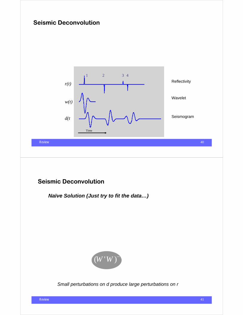
Review 39
S r
Depth
or Time
1
2
3
4
d(t) = w(τ - t)r(τ )dτ∫
Seismic Deconvolution
Review 40
d(t) = w(τ - t)r(τ )dτ∫w(t) = δ (t) ⇒ d (t) = r(r)
r(t)
w(t)
d(t)
Time
1 2 3 4
Reflectivity
Wavelet
Seismogram
Seismic Deconvolution
d = Wr
Review 41
Seismic Deconvolution
d = W r + n
J =||Wr − d ||22
∇J = W 'W r −W ' d = 0
ˆ r = (W 'W )−1W ' d
Small perturbations on d produce large perturbations on r
Naïve Solution (Just try to fit the data…)

Review 42
Seismic Deconvolution
d = W r + n
J =||Wr − d ||22
∇J = W 'W r −W ' d = 0
c I ≈ W 'W
ˆ r ≈ c−1W ' d
Some sort of “backprojection”
Low Resolution Solution:
Review 43
Seismic Deconvolution
d = W r + n
J =||Wr − d ||22 +µ || Lr ||2
2
∇J = W 'W r −W ' d + µL' L r = 0
ˆ r = (W 'W + µL' L)−1W ' d
L = I ⇒
ˆ r = (W 'W + µI)−1W ' d
Quadratic Regularization
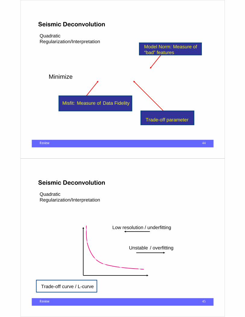
Review 44
Seismic Deconvolution
J =||Wr − d ||22 +µ || Lr ||2
2
Quadratic Regularization/Interpretation
Misfit: Measure of Data Fidelity
Model Norm: Measure of “bad” features
Trade-off parameter
Minimize
Review 45
Seismic Deconvolution
J =||Wr − d ||22 +µ || Lr ||2
2Quadratic Regularization/Interpretation
|| Lr ||22
||Wr − d ||22
µ = 104
µ = 10−6
∗∗
∗∗ ∗ ∗
Unstable / overfitting
Low resolution / underfitting
Trade-off curve / L-curve

Review 46
Seismic Deconvolution
L = I
L = D1
L = D2
D1, D2
zero order quadratic regularization (smallest model)
First order quadratic regularization (flattest model)
Second order quadratic regularization (smoothest model)
Are high pass operators (First and Second order Derivatives)
Quadratic Regularization
Typical regularizers J =||Wr − d ||22 +µ || Lr ||2
2
Review 47
Seismic Deconvolution: Trying to squeeze resolutionvia mathematical tricks..
When in Doubt, Smooth
Sir Harold Jeffreys (Quoted by Moritz, 1980; Taken from Tarantola, 1987)
But…, I don’t want to smooth!
A geophysicist trying to resolve thin layers
Let’s see how one can avoid smoothing and resolution degradation..

Review 48
Seismic Deconvolution: Trying to squeeze resolutionvia mathematical tricks..
Super-resolution via non-quadratic regularization
J =||Wr − d ||22 +µR(r)
R(r)= | ri |i
∑
R(r)= | ri |i
∑ 2
R(r) = ln(1+ri
2
σ c2
)i
∑
L1 norm
Cauchy regularizer
Let’s study the Cauchy norm invrsion
L2 norm Quadratic Norm
Non Quadratic Norm
Non Quadratic Norm
Review 49
Seismic Deconvolution: Non-quadratic norms and sparse deconvolution
•Non-quadratic norms can be used to retrieve sparse models
•Sparse models area associated to broad-band solution
•A sparse-spike solution can be used to retrievedsparse reflectivity series which is equivalent to finding blocky impedance profiles
•Historically the problems arose in the context of impedance inversion (80’s)
- Claerbout, J. F., and F. Muir, 1973, Robust modeling with erratic data: Geophysics, 38, 826-844.
- Taylor, H. L., S. C. Banks, and J. F. McCoy, 1979, Deconvolution with the L-one norm: Geophysics, 44, 39-52.
- Oldenburg, D. W., T. Scheuer, and S. Levy, 1983, Recovery of the acoustic impedance from reflection
seismograms: Geophysics, 48, 1318-1337.

Review 50
Cauchy Norm Deconvolution
Super-resolution via non-quadratic regularization
J =||W r − d ||22 +µS(r)
S(r) = ln(1+ri
2
σ 2)
i∑
∇J = W 'W r −W ' d + µ Q(r) r = 0
r = (W 'W + µQ(r) )−1W ' dIRLS
Review 51
r = (W 'W + µQ(r) )−1W ' d
Qii =1
σ 2 (1+ ri2 /σ c
2)
Cauchy Norm Deconvolution
The problem is non-linear, the reflectivity depends on the reflectivity…
iter = 0r iter = 0
For iter = 1: iter_max
Qiterii =
1
σ c2 (1+ (ri
iter )2 /σ c2)
r iter+1 = (W 'W + µQiter )−1W ' d
End
Iterative Re-weighted Least Squares
Review 52
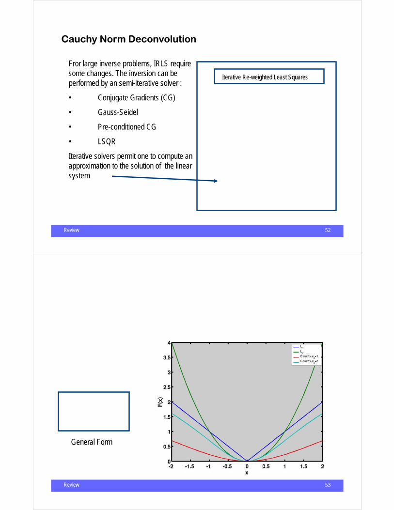
Cauchy Norm Deconvolution
Fror large inverse problems, IRLS require some changes. The inversion can beperformed by an semi-iterative solver :
• Conjugate Gradients (CG)
• Gauss-Seidel
• Pre-conditioned CG
• LSQR
Iterative solvers permit one to compute an approximation to the solution of the linear system
iter = 1r iter = 0
For iter = 1: iter_max
Qiterii =
1
σ c2 (1+ (ri
iter )2 /σ c2)
r iter+1 = (W 'W + µQiter )−1W ' d
End
Iterative Re-weighted Least Squares
Review 53
R(r)= | ri |i
∑
R(r)= | ri |i
∑ 2
R(r) = ln(1+ri
2
σ c2
)i
∑
R(r) = F (ri)i
∑
General Form
Review 54
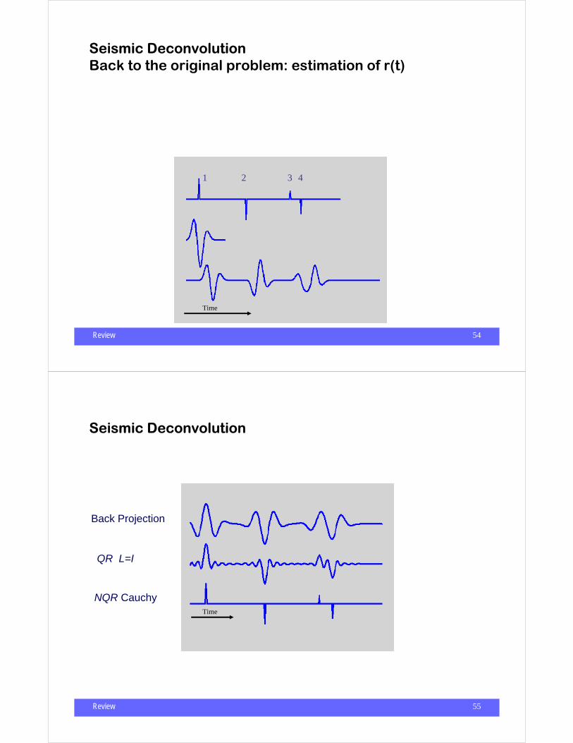
d(t) = w(τ - t)r(τ )dτ∫
r(t)
w(t)
d(t)
Time
1 2 3 4
Reflectivity
Wavelet
Seismogram
Seismic DeconvolutionBack to the original problem: estimation of r(t)
Review 55
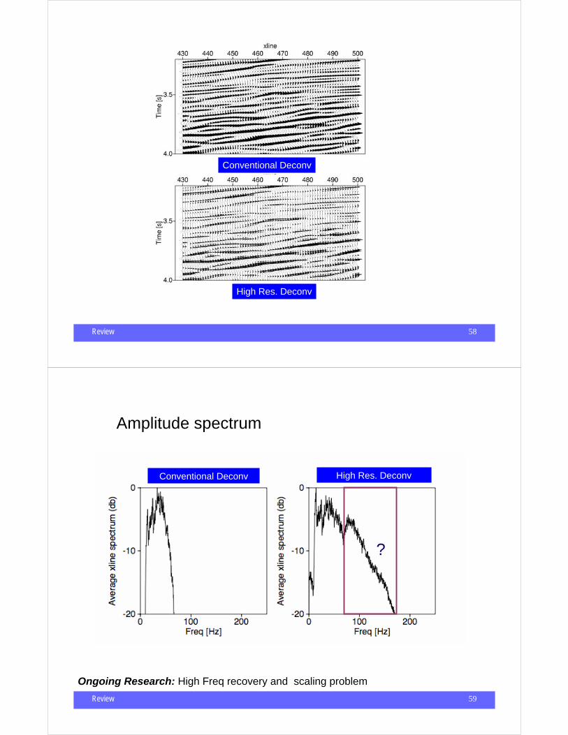
Back Projection
QR L=I
NQR Cauchy
Seismic Deconvolution
Time

Review 56
Back Projection
QR L=I
NQR Cauchy
Seismic Deconvolution
Time
True
Review 57
Conventional Deconv High Res. Deconv
3D Seismic Section from somewhere (HFR - High Freq. Restoration)
Review 58
High Res. Deconv
Conventional Deconv
Review 59
High Res. DeconvConventional Deconv
Amplitude spectrum
Ongoing Research: High Freq recovery and scaling problem
?
Review 60
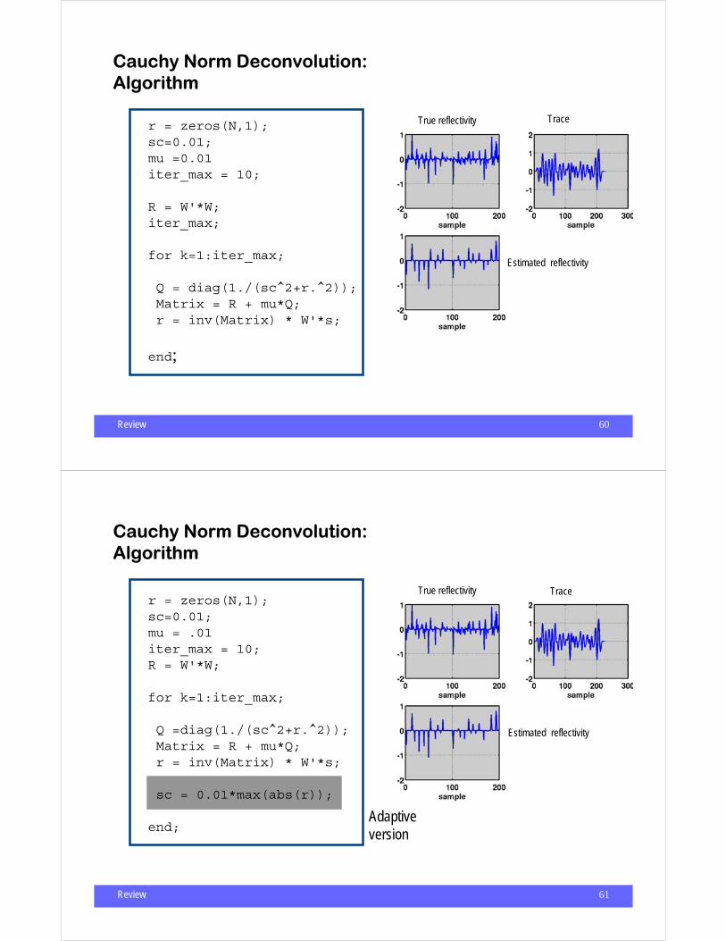
Cauchy Norm Deconvolution:Algorithm
r = zeros(N,1);sc=0.01; mu =0.01iter_max = 10;
R = W'*W;iter_max;
for k=1:iter_max;
Q = diag(1./(sc^2+r.^2));Matrix = R + mu*Q;r = inv(Matrix) * W'*s;
end;
True reflectivity Trace
Estimated reflectivity
Review 61
Cauchy Norm Deconvolution:Algorithm
r = zeros(N,1);sc=0.01;mu = .01iter_max = 10;R = W'*W;
for k=1:iter_max;
Q =diag(1./(sc^2+r.^2));Matrix = R + mu*Q;r = inv(Matrix) * W'*s;
sc = 0.01*max(abs(r));
end;Adaptive version
True reflectivity Trace
Estimated reflectivity

Review 62
High frequency imaging methods….
Other methods exits - they all attempt to retrieve a sparse reflectivity sequence:
Atomic Decompostion/Matching Pursuit / Basic Pursuit (like an L1)
Chopra, S., J. Castagna, and O. Portniaguine, 2006, Seismic Resolution and Thin-Bed ReflectivityInversion: Recorder, 31, 19-25. (www.cseg.ca)
Portniaguine, O., and J. P. Castagna, 2004, Inverse spectral decomposition: 74th AnnualInternational Meeting, SEG, Expanded Abstracts, 1786-1789.
Review 63
rk =Ik +1 − Ik
Ik +1 + Ik
ξk =1
2log(Ik / I0) ≈ rk
j= 0
k
∑
J =||W r − d ||22 +µS(r) + β || Cr −ξ ||2
2
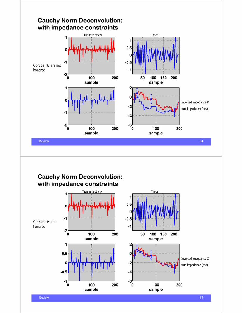
Cauchy Norm Deconvolution:with impedance constraints
Reflectivity as a function of P-impedance
Approximation
Fit the dataSolution must be sparse (High freq)
Fit impedance constraints
Review 64
Cauchy Norm Deconvolution:with impedance constraints
β = 0Constraints are not honored
True reflectivity Trace
Inverted impedance &
true impedance (red)
Review 65
Cauchy Norm Deconvolution:with impedance constraints
β = 0.25
Constraints are honored
True reflectivity Trace
Inverted impedance &
true impedance (red)

Review 66
beta=0.25iter_max=10R = W'*W+beta*C'*C;r = zeros(N,1);
for k=1:iter_max;Q = diag(1./(sc^2+r.^2));Matrix = R + mu*Q;r = inv(Matrix) * (W'*s+beta*C'*psi)sc = 0.01*max(abs(r));end;
Cauchy Norm Deconvolution:with impedance constraints - Algorithm
Review 67
AVO: Amplitude versus offset
AVA: Amplitude versus angle
AVP: Amplitude versus Ray Parameter
Estimation of rock properties & HCI
AVO
Review 68
α α
r(t,α, x) = f (x,α,v− ,v+ ,ρ− ,ρ+) = A(t, x) + B(t, x) × F (α)
d (t,α, x) = ∫ r(τ ,α, x) w(τ − t)dτ
v− ,ρ−
v+ ,ρ+
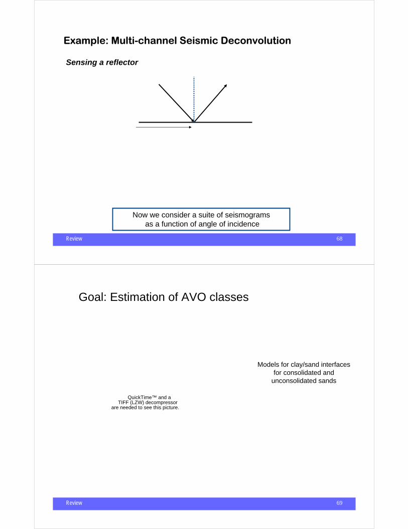
Example: Multi-channel Seismic Deconvolution
x
w(t) d (t,α, x)
Sensing a reflector
Now we consider a suite of seismogramsas a function of angle of incidence
Review 69
QuickTime™ and aTIFF (LZW) decompressor
are needed to see this picture.
Goal: Estimation of AVO classes
Models for clay/sand interfaces for consolidated and
unconsolidated sands

Review 70
ˆ A (t, x) ˆ B (t, x)
Quadratic regularization
L=I
ˆ A (t, x) ˆ B (t, x)
Cauchy Solution

ˆ A (t, x) ˆ B (t, x)
IIIIII
Identify gasbearing sand lens
Interpretation/
AVA Analysis
r(t,α, x) = f (x,α,v− ,v+ ,ρ− ,ρ+)
= A(t, x) + B(t, x) × F (α)
A
B
Review 73
Large inverse problems: Pre-stack depth Imaging
Structural Imaging -- Where ?Where ?
Imaging Angle Dependent Reflectivity -- Where and What ?Where and What ?
Wang J., Kuehl H. and Sacchi M.D., 2005, High-resolution wave-equation AVA imaging: Algorithm and tests with a data set from the Western Canadian Sedimentary Basin: Geophysics, 70, 891-899

Review 74
Imaging - Large scale problems
r(α, x,z)
x
z
SOURCE (s)
RECEIVER/GEOPHONE (g)
h
m
m: midpointh: offset
Wang, Kuehl and Sacchi, Geophysics 2005
α
We want the variation of the reflectivity at each subsurface position:
A 2D image is in fact a 3D volume
A 3D Image is a 5D Volume
Review 75
Imaging in Operator Form..
A m = d + n
m = m(x, y,z, p), p =sin(α)
v (x, y,z)
d = d (
g ,
s , t)
g = [gx ,gy ],
s = [sx ,sy ]
r(α, x,z)
d: is now pre-processed seismic data

Review 76
A r = d
rmig = A' d
rinv = A−1d
Modeling
Migration
Inversion
Migration/Inversion Hierarchy..
Review 77
Regularized Imaging
• We don’t have A, we only have a code that knows how to apply A to m and, another, that knows how to apply A’ to d
• A and A’ are built to pass the dot product test
• Importance of sampling Matrix W for reducing footprints (Kuehl, 2002, PhD Dissertation)
Remarks:
J=||W (Ar − d) ||22 +µR(r)
Migration
MigrationInversion
Review 79
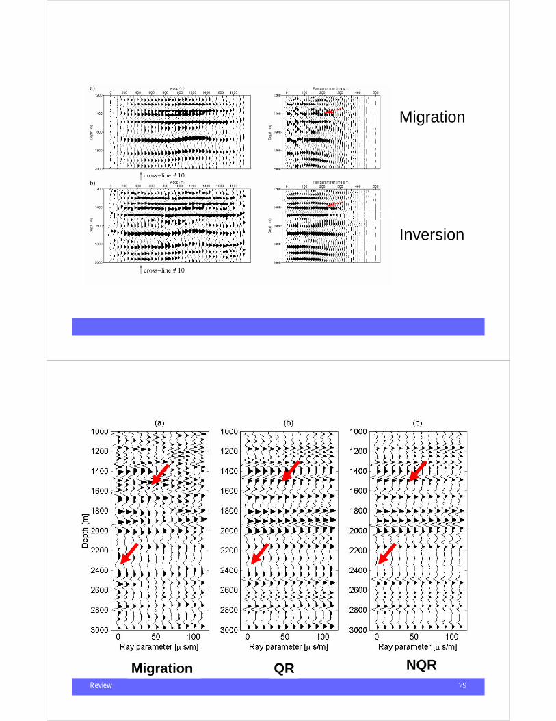
r = r(x = x' ,y = y' ,z, p),
Migration QR NQR
Review 80
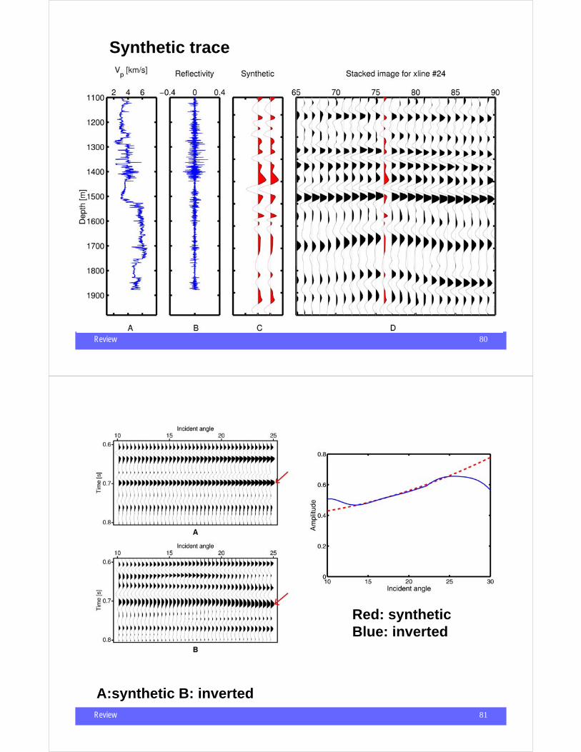
Synthetic trace
Review 81
A:synthetic B: inverted
Red: syntheticBlue: inverted