P-ADIC POLYNOMIAL DYNAMICS

AIHUA FAN

Abstract. This introductory lecture intends to present polynomial dynamics

on the ring Zp of p-adic integral numbers, a large class of topological symbolic

dynamics. Such symbolic dynamics can be studied as algebraic dynamics us-ing algebraic and analytic methods. To this end, we will first present p-adic

numbers and analysis on the filed Qp of p-adic numbers.

1. Introduction

Our objects of study are Cantor topological dynamical systems T : X → Xwhere T is a continuous map on a Cantor set X. Typically

X = {0, 1}∞.

We would like to consider (T,X) as an algebraic dynamics. By identifying 0, 1 with2Z, 1 + 2Z, we can consider X as

X = (Z/2Z)× (Z/2Z)× (Z/2Z)× · · · .

It is a group, an infinite product group. But we will consider another group op-eration on X. Better is that we can make X into a ring, a local ring and evenZ-module. So, continuous maps on X include polynomials which are dense in thespace of all continuous maps (Kaplansky). Calculus can also be well developed onsuch a local ring and on its fraction fields.

(1) Do the algebraic structure and the calculus helps us to understand thedynamics T : X → X ?

(2) How about the polynomial dynamics ?

Such dynamics are called dyadic dynamics and more generally we can considerp-adic dynamics for any prime p.

One of motivation for studying p-adic dynamics come from physics. Volovich [?]published the first paper on application of p-adic numbers to theoretical physics( p-adic string theory). The string theory attempts to reconsider foundations of physicsby using space extended objets (strings) instead of pointwise objects (elementaryparticles). The scenarios of string spectacle is performed at Planck distances (10−34

cm). Physicists have the feeling that the space-time at Planck scale have somedistinguishing features which cannot be described by the standard mathematicalmodels based on the Archimedean field R which has the following Archimedeanproperty:

` > 0, L > 0⇒ ∃n ∈ N, n` > L.

There were also intuitive cosmological ideas that the space-time at Planck scalehas non-Archimedean structure. On the other hand, at Planck scale, there wouldbe no order, not like on R. The field Qp of p-adic numbers has non-Archimedeanstructure and is non-ordered.

1

2 AIHUA FAN

The theory of p-adic dynamical systems is recently rapidly developing (see thebooks [4, 30, 32, 41, 49, 50]). Motivated by different parts of mathematics andphysics where it is natural to treat the p-adic completion of the field Q of rationalnumbers and to use this completed field (including number theory, algebraic andarithmetic geometry, cryptography, physical models, biological models, and so on).

The p-adic dynamics appears naturally in the study of smooth dynamics. Forexample, an ergodic algebraic automorphism of a torus preserving Haar measurewas shown by Katznelson [29] to be isomorphic to a Bernoulli shift which is of p-adic nature. This was generalized by Lind [36] to skew products with ergodic groupautomorphism where the understanding of the p-adic hyperbolicity was involved.See [?, 37, 38] for other situations where p-adic dynamics or p-adic considerationarise.

It seems that the first study of p-adic dynamical systems is the work of Oseliesand Zieschang [44] where they considered the continuous automorphisms of the ringof p-adic integers Zp viewed as an additive group, which are multiplication trans-formations Ma(x) = ax with a ∈ Z×p , a unit in Zp. They constructed an ergodic

decomposition of Ma : Z×p → Z×p which consists of the cosets of the smallest closed

subgroup containing a of the unit group Z×p . These multiplication transformationswere also studied by Coelho and Parry [13] in order to study the distribution ofFibonacci numbers. The simple power transformations ψn(x) = xn acting on thegroup of units Z×p were studied by Gundlach, Khrennikov and Lindahl [25]. Hermanand Yoccoz ([26]) proved that Siegel’s linearization theorem in complex dynamicalsystems is also true for non-Archimedean fields. Their work might be the first oneon complex p-adic dynamics. Lubin [40] used the formal groups from local arith-metic geometry to study iterates of p-adic analytic maps. Li [35], Benedetto [9],Hsia [27], Rivera-Letelier [46], Jones [28] and others have systematically studiediteration of rational maps over the p-adic Riemann sphere. In a different direc-tion, Morton and Silverman [43], Arrowsmith and Vivaldi [6] and others have alsostudied arithmetic dynamics using p-adic techniques.

In this lecture, we first introduce p-adic numbers and present basic notions ofp-adic analysis. Then we present two kinds of polynomial dynamics, one is chaoticand the other is 1-Lipschitz.

2. Random number generators

We need random numbers. p-adic dynamics are related to random number gen-eration and to cryptography etc.

2.1. von Neumann method. The middle-square method is a method of gener-ating pseudorandom numbers, a first method. The method was first described ina manuscript by a Franciscan friar (known as Brother Edvin) between 1240 and1250. John von Neumann reinvented it and described it at a conference in 1949.The method is defined by the function N taking the middle k-digit number of thesquare of an integer.

Here is the method: take a seed a0: a k-digit number.define the recurrencean+1 = N(an): the middle k-digit number of a2

n.There are bad seeds (k = 4) like 0100, 2500, 3792, 7600. For example, 3792 is fixedby N :

37922 = 143972 64, 3972 = N(3972)

P-ADIC POLYNOMIAL DYNAMICS 3

The following seeds (n = 4) 0540, 2916, 5030, 3009 are good. Actually 0540 →9160 → 9056 → 0111 → 1232 → 5178 → 8116 → 8994 → 8920 → 5664 → 0808 →5386 → 0089 → 7921 → 7422 → 0860 → 3960 → 6816 → 4578 → 9580 → 7764 →...

How to find cycles as long as possible ? This method is not a good method, sinceits period is usually very short.

2.2. Linear Congruently Generator (ECG). The linear congruently generatormethod represents one of the oldest and best-known pseudorandom number gen-erator algorithms. The method is easy to understand and easy implement. Thegenerator is defined by the recurrence relation:

Xn+1 = aXn + b mod m (n ≥ 0)

where

• m ≥ 2: modulus• a: multiplier• b: increment• X0: seed

Remark that Xn ∈ {0, 1, · · · ,m − 1} = Z/mZ and Xn/m ∈ {0/m, 1/m, · · · , (m −1)/m} ⊂ [0, 1]. We consider Xn/m as pseudorandom number. {Xn} is an orbit.One problem is to find maximal period of the system, which is smaller than ≤ m.

Is Xn/m a sample of U(0, 1) (the uniform distribution on the interval [0, 1]) ?Non, it is not and can only consider it as pseudorandom.

Here comes the first dynamical system to study: the affine dynamics x 7→ ax+b (mod m), which is a finite dynamical system on the ring Z/mZ.

2.3. A simple algebraic dynamics (warmup). Notice that Z/pZ is a field.Computations below are made in the field. For example, a = 1 means a = 1 (modp) and a−1 mean the inverse in the field.

Theorem 1. Ta,bx = ax+ b is minimal on Z/pZ iffy a = 1 and b 6= 0.

Proof. Necessity. If b = 0, 0 would be a fixed point. Contradiction. If a 6= 1,1−a would be invertible. Then we solve Ta,bx = x and get a fixed point (1−a)−1b.Contradiction.

Sufficiency. Since a = 1, Ta,bx = x+b. It is clear that the orbit of 0: 0, b, · · · , (p−1)b is a full cycle if b 6= 0. �

Let us make some remarks:

• It seems too simple. But conveniently choose b (large enough, but not toolarge), we see some randomness it the orbits. For example, the orbit of 0for 12x+ 5 on Z/11Z:

0, 5, 10, 4, 9, 3, 8, 2, 7, 1, 6

• It is not so simple on the ring Z/mZ for general m.• On any ring, we have

T ka,bx = akx+ (1 + a+ · · ·+ ak−1)b = akx+ak − 1

a− 1b

(assuming a − 1 is invertible for the last equality). So the behavior of thepowers ak play a role.

4 AIHUA FAN

The following simple analysis gives a full picture of the dynamics of Ta,b on Z/pZ.

Theorem 2. Consider an arbitrary affine mapping Ta,bx = ax+ b.

(1) If a = 0, there is one fixed point b who attracts all other points.(2) If a = 1 and b = 0, there are p fixed points.(3) If a = 1 and b 6= 0, there is a (maximal) cycle.(4) If a 6= 0, 1 (having d as its order), there is one fixed point −b/(a − 1) and

(p− 1)/d cycles of length d.

Proof. Only the last point needs a proof. For any k ≥ 1

T ka,bx− x = (ak − 1)

(x+

b

a− 1

).

So T ka,bx = x iff x+ b/(a− 1) = 0 or ak − 1 = 0. The least such k is the order of a,

which is independent of x (6= −b/(a− 1)). �How to do with higher order polynomial generator ?

3. Ring of integer-valued polynomials Int(Z)

Integer-valued polynomials were studied by Polya (see [10]). We say that P ∈Q[x] is an integer-valued polynomials (we write P ∈ Int(Z)): if P (Z) ⊂ Z. Exam-

ples: x(x−1)2 , x(x+1)(x+2)

6 . Typical examples:

B0(x) ≡ 1, Bn(x) =x(x− 1)(x− 2) · · · (x− n+ 1)

n!=

(x

n

).

Theorem 3 (Polya). {Bk}0≤k≤n is a basis of the Q-vector space Qn[x]. It is alsoa basis of the Z-module Intn(Z) = Int(Z) ∩Qn[x].

Proof The first assertion follows from the basic properties of Bn:

• degBk = k.• If 0 ≤ k < n, Bn(k) = 0 (all zeros of Bn).• If k > n, Bn(k) ∈ N∗ (choose n from k)• If x < 0, Bn(k) = (−1)nBn(n+ |k| − 1) ∈ Z.

For the second assertion, we need to observe that Bk ∈ Int(Z). �Conclusion: f ∈ Int(Z) with degf = n iff there exists (unique) (a0, a1, · · · , an) ∈

Zn+1 such that

f(x) =

n∑k=0

ak

(x

n

).

How to find a0, a1, · · · , an ? The Gregory-Newton interpolation gives a solution.Define the (forward) difference operator

∆f(x) = f(x+ 1)− f(x)

and the translation operator

Tf(x) = f(x+ 1).

They have the relations:

∆ = T − I, ∆n = (T − I)n =

n∑k=0

(−1)n−k(nk

)T k.

P-ADIC POLYNOMIAL DYNAMICS 5

So,

∆nf(x) =

n∑k=0

(−1)n−k(nk

)f(x+ k).

Theorem 4 (Gregory-Newton). For f ∈ Rn[x], we have

f(x) =

n∑k=0

∆kf(0)Bk(x).

Proof It is a consequence of the facts: Bn(k) = δn,k for 0 ≤ k ≤ n); ∆Bn = Bn−1

(B−1 ≡ 0) which is a consequence of Pascal relation; and

∆kf(x) = akB0(x) + ak+1B1(x) + · · ·+ anBn−k(x).

�This result will be generalized to the Mahler expansion of p-adic continuous

functions.

4. p-adic Numbers

In this section, we construct from different ways the field Qp of p-adic numbersand we prove a first theorem in the p-adic analysis, namely the theorem on Mahlerexpansions in C(Zp,Qp) which is the space of all continuous functions defined onZp taking values in Qp. The result is a generalization of the above mentioned Polyatheorem. See [42, 47, 48] for the theory of p-adic numbers.

4.1. Systems of numbers constructed from N. Suppose that we are givena sequence of positive integers (m0,m1, · · · ,mk, · · · ) with mk ≥ 2. The mostimportant case is mk = p for all k, where p is a prime. We claim that

N '∐{0, 1, · · · ,mk − 1}.

In other word, for any integer n ∈ N, there exists unique ak ∈ {0, 1, · · · ,mk − 1}such that

(1) n = a0 + a1m0 + a2m0m1 + · · ·+ aNm0m1 · · ·mN−1.

We can actually find the ak’s (called digits) recursively by the Euclidean algorithm:

(Euclid) n = m0n′ + a0, n′ = m1n

′′ + a1, · · · .We define the product space

Z(mk) :=

∞∏k=0

Z/mkZ.

For x = (a0, a1, · · · ) ∈ Z(mk), we can formally write

(2) x =

∞∑k=0

akm0 · · ·mk−1.

Actually, as we will see, the series converges with respect to a metric which iscompatible with the product topology. The space Z(mk) is compact, by Tychonov’stheorem.

We have the embedding N ⊂ Z(mk)?according to (1) and N is evidently dense in

Z(mk) (i.e. N = Z(mk)).

6 AIHUA FAN

For the special case mk = p, we denote special Z(mk) with mk = p by Zp. Inthis case, we have the (formal) expansion

x =

∞∑k=0

akpk.

4.2. Z(mk) is a ring. Addition and multiplication are defined in N, which is densein Z(mk). These operations defined from N × N into N are uniformly continuous.So, they can be uniquely extended on Z(mk).

How to add and multiply two positive integers using their digits? Just as usual,we manipulate (add or multiply) the digits with carry to the right. In the same wecan add and multiply two ”numbers” in Z(mk) by manipulating their digits withcarry to the right. For example,

(1, 0, 0, · · · ) + (m0 − 1,m1 − 1,m2 − 1, · · · ) = (0, 0, 0, · · · ).Recall that

1 = (1, 0, 0, · · · )So, we could say that

−1 = (m0 − 1,m1 − 1,m2 − 1, · · · ).

Theorem 5. Z(mk) is a ring. In particular, Zp is a ring.

Proof. Clearly, 0 = (0, 0, · · · ) is the neutral element of the addition and 1 =(1, 0, · · · ) is the unit of the multiplication. The commutativity, associativity anddistributivity are consequences of those in N. It is easy to check that

−(a0, a1, ak, · · · ) = (m0 − a0 − 1,m1 − a1 − 1,m2 − a2 − 1? · · · ).�

The proof shows that Z ⊂ Z(mk). But any strictly negative integer has infinitelymany non zero digits.

The mapping on Z(mk) defined by x 7→ x+ 1 s called the Odometer on Z(mk).

4.3. Field of p-adic numbers. If mk = p for some prime p, we get a betterstructure.

Theorem 6. Let p ≥ 2 be a prime. Then Zp is an integral ring. An element∑∞k=0 akp

k ∈ Zp is invertible iff a0 6= 0.

Proof. The commutative ring Zp contains Z as subring. We are going to showthat it has no zero divisor. Let

a =

∞∑k=0

akpk 6= 0, b =

∞∑k=0

bkpk 6= 0.

Define u (respectively v) to be the first k such that ak 6= 0 (respectively bk 6= 0).Then au and bv are not divisible by p, and then so is anbv. By definition ofmultiplication, the first nonzero digit cu+v of the product ab is the digit associatedto pu+v and it is defined by

0 ≤ cu+v < p, cu+v = aubv( mod p).

Since aubv is not divisible by p, we have cu+v 6= 0, so that ab 6= 0.If a is invertible and b is its inverse, the above proof shows that we must have

u = v = 0, in particular u = 0. Now suppose u = 0. Choose 0 < b0 < p such that

P-ADIC POLYNOMIAL DYNAMICS 7

a0b0 = 1(mod p). So we can write a0b0 = 1 + kp for some integer 0 ≤ k < p. Nowif we write a = a0 + pα, then

ab0 = 1 + kp+ pαb0 = 1 + pβ

for β ∈ Zp. We claim that it suffices to show that 1 + pβ is invertible, becausea · b0(1 + pβ)−1 = 1. So we get

a−1 = b0(1 + pβ)−1.

For the inverse of 1 + pβ, we can formally take

(l + pβ)−1 = 1− pβ + p2β2 − · · · = 1 + c1p+ c2p2 + · · · .

with 0 ≤ cj < p. We can surely find cj ’s by applying the rules for carries, althoughthe procedure is cumbersome. �

For example, 1− p is invertible in Zp. Actually we have

(1− p)−1 =1

1− p= 1 + p+ p2 + · · · ∈ Zp.

Elements in Zp are called p-adic integers. The sets N and Z are both dense subsetof Zp. By definition, the field of p-adic numbers, denoted by Qp, is the fractionfield of Zp. The following theorem provides a canonical representation for p-adicnumbers.

Theorem 7. Let x ∈ Qp be a p-adic number. Then there exists an integer v(x) ∈ Zsuch that

x =

∞∑i=v(x)

aipi

where ai ∈ {0, 1, · · · , p− 1} for all i with av(x) 6= 0. This expansion is unique. Therules of addition and multiplication in Qp is the same as in Qp.

Proof. Assume x 6= 0. Otherwise v(x) = −∞ and ak = 0 for all k. Bydefinition, there are z1, z2 ∈ Zp such that x = z1

z2. We can assume that z1 = p−va

for some v ∈ Z and z2 = b where

a =

∞∑k=0

akpk, b =

∞∑k=0

bkpk

with a0 6= 0 and bk 6= 0. Then a, b ∈ Zp and b is invertible in Zp. So ab ∈ Zp. Write

a

b=

∞∑k=0

ckpk.

Thus

x = p−v∞∑k=0

ckpk =

∞∑n=v

cn+vpn.

The uniqueness of the expansion is left as exercise. For the above number x, aftermultiply x by pv we get a p-adic integer xpv. This fact allows us immediately tounderstand how operate the addition and the multiplication. �

If x has the above expansion, the following fraction

{x} :=∑

v(x)≤i<0

aipi

8 AIHUA FAN

is called the fractional part of x. While x− {x} is the integral part of x.

It is easy to see that the shift on Zp has the following algebraic expression:

(x0, x1, · · · ) 7→ σp(x) = (x1, x2, · · · ) =x

p−{x

p

}.

Thus, we could consider the shift as an ”algebraic” dynamics. But it is not poly-nomial in the strict sense.

As we shall see, odometers and shifts are prototypes of our algebraic dynamicalsystems.

4.4. Norm and valuation on Qp (second way of introducing Qp). Now letus explain the second way to construct the field of p-adic numbers. The usual fieldR of real numbers is the completion of the field Q of rational numbers relative tothe usual absolute value | · |.

We can construct the field Qp in the same way but with another absolute value(also called norm).

The p-adic norm of a rational number x ∈ Q, denoted by |x|p, is defined asfollows:

|x|p = p−vp(x) if x = pvp(x) r

swith (r, p) = (s, p) = 1

where the integer vp(x) is called the p-adic valuation of x.It is not difficult to check that |x|p is a non-Archimedean norm in the sense that

• | − x|p = |x|p• |xy|p = |x|p|y|p• |x+ y|p ≤ max{|x|p, |y|p}

The last inequality is called ultra triangle inequality, which implies that there areonly isocele triangles in (Q, | · |p).

Theorem 8 (Ostrowski). Each non-trivial norm on Q is equivalent to | · | or to| · |p for some prime p.

By definition, the field of p-adic numbers Qp is the | · |p-completion of Q.The fields C of complex numbers is the quadratic extension R(i) of R. The

field C is topologically complete and algebraically closed. But no finite extensionQp(α1, · · · , αr) is algebraically closed. Take an algebraically closed extension Qacp .The completion of Qacp is denoted Cp which is topologically complete and alge-braically closed. We call Cp the field of ”complex” p-adic numbers.

As a vector space over Qp, Cp has an infinite dimension. Also notice that, unlikeC, Cp is not locally compact.

4.5. Properties of Zp and Qp (Third point of view). The ring Zp is equal tothe inverse limit

Zp ← · · · ← Z/pn+1Z← Z/pnZ← · · · ← Z/pZ.

In other word, z ∈ Zp is identified with (zn) ∈∏∞n=1 Z/pnZ such that

zn+1 = zn ( mod pn).

We can actually take zn =∑n−1k=0 p

kak when z =∑∞k=0 p

kak.Let us give the following list of properties:

P-ADIC POLYNOMIAL DYNAMICS 9

(1) We have

Zp = {x ∈ Qp : |x|p ≤ 1}and the closed (open) ball Bp−k(a) centered at a of radius P−k equals

a+ pkZp.(2) U := {x ∈ Zp : |x|p = 1} is the group of units of Zp and

U =

p−1⊔i=1

B1/p(i).

(3) P = {x ∈ Zp : |x|p < 1} = B1/p(0) is the unique maximal ideal of Zp.(4) |Q∗p|p = {pk : k ∈ Z} a discrete subgroup of (R∗+,×).(5) Qp is separable, locally compact and totally disconnected.

4.6. Legendre formula. Let us present the Legendre formula. Its proof showshow to compute the valuation of a number.

Theorem 9. Write n =∑tk=0 akp

k. Then

vp(n!) =

∞∑j=1

⌊n

pj

⌋=n− sp(n)

p− 1

where sp(n) =∑tk=0 ak.

Proof. Consider the sequence {1, 2, · · · , n}. The subsequence of bn/pc elements

p, 2p, · · · , bn/pcpis compose of those divisible by p, and that of bn/p2c elements

p2, 2p2, · · · , bn/p2cp2

is composed of those divisible by p2 (an element in both sequences will be accountedtwice), and so on. Thus the first equality is proved. Notice that⌊

n

pj

⌋= aj + aj+1p+ · · ·+ atp

t−j = p−j(ajpj + · · ·+ atp

t).

Then vp(n!) is equal to

t∑j=1

p−jt∑i=j

aipi =

t∑i=1

aipi

i∑j=1

p−j =p−1

1− p−1

t∑i=0

(1− p−i)aipi =n− sp(n)

p− 1.

�

4.7. Mahler expansion. Continuous functions on Zp taking values in Qp are de-scribed by the following theorem.

Theorem 10. Any f ∈ C(Zp → Qp) is uniquely expanded as

f(x) =

∞∑n=0

an

(x

n

)where

an = 4nf(0) =

n∑j=0

(n

j

)(−1)n−jf(j).

10 AIHUA FAN

Proof. Recall that Tf(x) = f(x+1), 4f(x) = f(x+1)−f(x). Thus4 = T−I.Then

4n = (T − I)n =

n∑j=0

(n

j

)(−1)n−jT j .

Since f ∈ C(Zp → Qp) is uniformly continuous, we have limωn(f) = 0 where

ωn(f) := sup|x−y|p≤p−n

|f(x)− f(y)|p.

For x ∈ Zp, we have

∆nf(x) =

n∑k=0

(−1)n−k(n

k

)[f(x+ k)− f(x)]

(Notice that the sum of coefficients equals to zero because of (1 − 1)n = 0). For

0 ≤ k ≤ pn we have |(pn

k

)|p = p−n+vp(k) (Exercise, try by Legendre formula) so

that ∥∥∥∆pnf∥∥∥∞≤ max

0≤s≤np−n+sωs(f)→ 0.

Then ∆nf converges uniformly to zero (using ‖∆g‖∞ ≤ ‖g‖∞) so that

an := ∆nf(0)→ 0.

On the other hand,

∀x ∈ N, f(x) =

∞∑n=0

an

(x

n

).

(it is a finite sum). We finish the proof by using the fact that N is dense in Zp. �

5. p-adic analysis

5.1. Sequence, Series, Continuity, Derivative. (Qp, |·|p) is a complete normedfield. Notions like limit of a sequence, convergence of a series and continuity of afunction are ”classical”. The ultra-metric inequality makes things simpler in p-adicworld, and sometimes different.

A sequence (an) ⊂ Qp is a Cauchy sequence iff limn→∞ |an+1 − an|p = 0. Aseries

∑∞n=1 an converges iff limn→∞ an = 0. Cauchy-Hadamard formula holds for

Taylor series∑∞n=0 anx

n.The derivative is defined formally as usual:

f ′(a) = limh→0

f(a+ h)− f(a)

h.

But the space C1 of continuously differentiable function is not a ”good” space.

(1) Locally constant functions admits zero derivatives. There are even injectivemaps having zero derivative: f(x) =

∑∞n=0 xnp

2n for x =∑∞n=0 xnp

n ∈ Zp.We have |f(x)− f(y)|p = |x− y|2p.

(2) The mean value theorem doesn’t holds in C1(Zp → Qp):

f(x)− f(y) = f ′(ξ)(x− y) (for some ξ between x and y)

[Between means ξ = tx+ (1− t)y with |t|p ≤ 1].

P-ADIC POLYNOMIAL DYNAMICS 11

5.2. Strict differentiability. We define a stronger differentiability. Let f : U →Qp be defined on an open set and a ∈ U . We say f is strictly differentiable at a ifthe limit exists:

f ′(a) = lim(x,y)→(a,a),x 6=y

f(x)− f(y)

x− y.

We denote by C1s (U → Qp) ⊂ C1(U → Qp the space of all functions defined and

strictly differentiable in U taking values in Qp.We remark that

(1) C1s (U → Qp) ⊂ C1(U → Qp (strict inclusion).

(2) f ∈ C1s (U → Qp) iff there exists R ∈ C(U × U → Qp) such that

f(x)− f(y) = (x− y)R(x, y).

Then we must have R(a, a) = f ′(a).(3) Lip1+δ(U → Qp) ⊂ C1

s (U → Qp).(4) analytic functions are strictly differentiable.

Theorem 11 (local injectivity). Let f ∈ C1s (U → Qp) and a ∈ U . Suppose

f ′(a) 6= 0, then there is an neighborhood V of a such that

∀x, y ∈ V, |f(x)− f(y)|p = |f ′(a)|p|x− y|p.

Proof. Directly from the definition and the fact f ′(a) 6= 0. For x and y close toa, we have ∣∣∣∣f(x)− f(y)

x− y− f ′(a)

∣∣∣∣p

< |f ′(a)|p.

�As an example, let us examine the differentiability of the shift σp. The shift map

σp is derivable and even strictly derivable and

σ′p(x) =1

p

In fact, the shift σp is locally affine:

σp(x) =

p−1∑j=0

(x

p− j

p

)1[j](x).

The differentiability follows immediately. So does the strict differentiability, becausewhen |x− y| ≤ p−1 we have

σp(x)− σp(y) =x− yp

.

But σp is not analytic at 0.

5.3. Newton Approximation and Local invertibility.

Theorem 12 (Newton Approximation). Let f : Br(a)→ Qp. Suppose there existss ∈ Qp such that

supx,y∈Br(a);x 6=y

∣∣∣∣f(x)− f(y)

x− y− s∣∣∣∣p

< |s|p.

Then s−sf is an isometry, which maps any ball Br′(b) onto B|s|pr′(f(b)), wherer′ ≤ r.

12 AIHUA FAN

Proof. The condition implies

|f(x)− f(y)|p = |s||x− y|p.Then the isometry follows. Consequently

f(Br′(b)) ⊂ B|s|pr′(f(b)).

For c ∈ f(Br′(b)), we shall find a zero of f(x)− c in Br′(b) by the Newton method:let

g(x) = x− s−1(f(x)− c).Actually g : Br′(b)→ Br′(b) is an contraction and admits a fixed point. �

In particular, if f is strictly differentiable and f ′(a) 6= 0, then we can locallyinverse the mapping f .

Theorem 13 (Local invertibility). Let f : Br(a) → Qp be strictly differentiable.Suppose f ′(a) 6= 0. Then for sufficiently small r′, f : Br′(a) → B|f ′(a)|pr′(f(a)) isa diffeomorphism and

(f−1)′(f(a)) = (f ′(a))−1.

Proof. Apply the above lemma with s = f ′(a). g := f−1 is a scalar multiple ofan isometry and it is then continuous. For z, w ∈ B|f ′(a)|pr(f(a)), we have

g(z)− g(w)

z − w=

(f(g(z))− f(g(w))

g(z)− g(w)

)−1

.

It follows the strict differentiability of g at f(a). �

5.4. Analytic functions, exponential and logarithmic functions. As usual,a function f defined in a disk D is analytic if there exists u ∈ D such that

f(x) =

∞∑n=0

an(x− u)n,∀x ∈ D.

A function f defined in an open set U is locally analytic function if for any a ∈ U ,f is analytic in a disk containing a.

Theorem 14 (non analytic continuation by power series). If f is analytic in a diskD, then for any v ∈ D, f(x) is equal to some power series

∑∞n=0 bn(x−v)n around

v for all x ∈ D.

Let us make the following remarks:

(1) If f(x) =∑∞n=0 an(x− u)n,∀x ∈ D, then ann! = f (n)(u).

(2) The zeros of an analytic function don’t have accumulation points.(3) Composition of analytic functions are not necessarily analytic. Counter

example: f(x) = xp − x is analytic in Zp taking values in pZp and g(x) =(1− x)−1 is analytic in pZp. But g ◦ f is not analytic in Zp.

(4) Composition is stable for locally analytic functions.

The exponential function on Qp is defined formally as usual:

expx =

∞∑n=0

xn

n!.

A big difference from usual analysis is that the p-adic exponential function is notdefined on the whole space Qp. Let us recall the Legendre formula, which is useful to

P-ADIC POLYNOMIAL DYNAMICS 13

determine the domain of convergence of the series defining the exponential function.Let sp(n) be the sum of p-adic digits of n. Then

vp(n!) =

∞∑j=0

⌊n

pj

⌋=n− sp(n)

p− 1.

Here are some properties of the exponential function:

• Domain of convergence: E = {x : |x|p < p−1/(p−1) < 1}.• E = pZp for p 6= 2 (1/p < 1/(p− 1) < 1);E = 4Z2 for p = 2 (1/(p− 1) = 1, divergence at x = 2).• exp(x+ y) = expx exp y (∀x, y ∈ E).• (expx)′ = expx.• | expx− 1|p < 1. The image of E under exp is 1 + E.

The Logarithm function on Qp is defined formally as usual:

log x =

∞∑n=1

(−1)n+1 (x− 1)n

n.

The estimate vp(n) = O(log n) (or for pvp(n) ≤ n) is useful to determine thedomain of convergence of the series defining the logarithmic function.

Here are some properties of the logarithmic function:

• Domain of convergence: L = {x : |x− 1|p < 1} = 1 + pZp.• log(xy) = log x+ log y (∀x, y ∈ L).• (log x)′ = 1/x.• ∀x ∈ 1 + E, | log x|p < p−1/(p−1).

The image of 1 + E under log x is E.• log expx = x (∀x ∈ E); exp log y = y (∀y ∈ 1 + E).• exp and log are isometries, respectively on E and 1 + E.

5.5. Hensel lemma. Hensel lemma is a very useful tool for finding zeros of ananalytic or polynomial function.

Theorem 15 (Hensel Lemma). Let f be analytic in Zp, given by

f(x) =

∞∑n=0

anxn.

Suppose that

|an|p ≤ 1, |f(a)|p < 1, |f ′(a)|p = 1

for some a ∈ Zp. Then f admits a (unique ) zero b ∈ Zp such that |b−a|p ≤ |f(a)|p.

Proof. Assume r := |f(a)|p > 0 (otherwise, b = 0). We shall apply thelemma of Newton approximation to f |Br(a) and s = f ′(a). First develop f at a:

f(x) =∑∞n=0 bn(x− a)n (|x|p ≤ 1). Observe that b0 = f(a), b1 = f ′(a), |bn|p ≤ 1.

Then for x, y ∈ Br(a) with x 6= y,∣∣∣∣f(x)− f(y)

x− y− f ′(a)

∣∣∣∣p

=

∣∣∣∣∣∞∑n=2

bn(x− a)n − (y − a)n

x− y

∣∣∣∣∣p

.

Let u = x− a and v = x− b. We have u 6= v, |u|p ≤ r, |v|p ≤ r.

14 AIHUA FAN

The last sum is then bounded by

supn≥2

|un − vn|p|uv|p

≤ supn≥2

rn−1 = r = |f(a)|p < 1 = |f ′(a)|p.

The Newton Approximation lemma shows that f : Br(a)→ Br(f(a)) is surjective.But 0 ∈ Br(f(a)). So there is a b ∈ Br(a) such that f(b) = 0. �

Theorem 16 (Hensel lemma for polynomials). Let P ∈ Zp[x]. Suppose there existsβ ∈ Zp such that

P (β) = 0 ( mod p), P ′(β) 6= 0 ( mod p).

Then there exists a unique α ∈ Zp such that

α = β ( mod p), P (α) = 0.

5.6. Integration and Antiderivative. There is no Newton-Leibniz formula forthe p-adic analysis. There is no Qp-valued Lebesgue measure.

∫f(x)dx is not well

defined as usual.We say that f is an antiderivative of f ′ if f ′ exists. If f admits an antiderivative

F , so is F + g for every locally constant g.

Theorem 17 (Dieudonne). Each f ∈ C(Zp → Qp) admits an antiderivative.

Theorem 18 (No Lebesgue measure). Additive, translation invariant and boundedQp-valued measure µ on clopens of Zp is the zero measure.

Proof. For each n, Zp is the disjoint union of a+ pnZp (0 ≤ a < pn). Then weget µ(Zp) = pnµ(pnZp). The boundedness implies

µ(Zp) = limnpnµ(pnZp) = 0.

Thus µ(a+ pnZp) = µ(pnZp) = p−nµ(Zp) = 0. �Here is a version of p-adic Riesz representation. This can be generalized to

compact ultrametric spaces.Let X ⊂ Qp be compact. Let A = A(X) be the set of all clopens of X.An integral on C(X → Qp) is by definition a continuous linear functional on

C(X → Qp), i.e. an element of C(X → Qp)′. A measure is by definition afunction µ : A → Qp which is finitely additive, and bounded in the sense

‖µ‖ = supK∈A

|µ(K)|p <∞.

Let M(X → Qp) denote the set of measures.

Theorem 19 (p-adic Riesz representation). The C(X → Qp)′ of integrals is iso-metrically isomorphic to the space M(X → Qp) of measures. The isomorphismφ 7→ µφ is defined by

µφ(K) = µ(1K).

The so-called Volkenborn integral is a different integral. It is a functional onC1s (Zp → Qp) but not on C(Zp → Qp).Let us first recall the following general principle of interpolation. Any uniformly

continuous map from N to Qp uniquely extends to a continuous function in C(Zp →Qp).

P-ADIC POLYNOMIAL DYNAMICS 15

Theorem 20. Let f ∈ C(Zp → Qp) be a continuous function. The function definedon N by

F (0) = 0, F (n) = f(0) + f(1) + · · ·+ f(n− 1)

is uniformly continuous. The extended function is denoted by Sf(x) (called indefi-nite sum of f). If f is strictly differentiable, so is Sf .

The Volkenborn integral of f ∈ C1s (Zp → Qp) is defined by the ”Riemann sum”∫

Zpf(x)dx = lim

n→∞p−n

pn−1∑j=0

f(j) = limn→∞

Sf(pn)− Sf(0)

pn= (Sf)′(0).

5.7. Fourier Analysis. Here we would like to present a Fourier analysis of func-tions defined in the field of p-adic numbers but taking values in the field of usualnumbers. So it is a special case of commutative harmonic analysis. We need toknow what are the group characters.

A character of the group (ZP ,+) is a continuous function γ : Zp → C such that|γ(z)| = 1 for all z ∈ and

γ(z1 + z2) = γ(z1)γ(z2) (z1, z2 ∈ Zp).

The set of all continuous characters, denoted by Zp, is a group for the usual point-wise multiplication.

Define

γn,k(z) := exp(2iπ{ kpnz}), (n > 1, pn > k > 1, p - k).

Theorem 21. Zp = {1} ∪ {γn,k}.Proof. Each γn,k is a character because

• {x+ y} = {x}+ {y} ( mod Z).• Zp 3 x 7→ R is locally constant then continuous.

Let γ ∈ Zp. We have γ(1) = e2iπθ for some θ ∈ [0, 1) and γ(pn) = γ(1)pn

.

γ continuous, pm → 0⇒ limm→+∞

exp(2iπpmθ) = limm→+∞

γ(pm) = γ(0) = 1.

Write θ =∑+∞j=1

θjpj (0 6 θj < p).

exp(2iπpmθ)→ 1⇒ limm→∞

θmθ = limm→∞

+∞∑j>m

θjpj−m

= 0.

It follows that the digit θm ends with 0’s. Write

θ = 0 or θ = k/pn (pn > k > 1, p - k).

Now for any z =∑+∞j=0 zjp

j ∈ Zp, we have

γ(z) = limN→+∞

γ(

N∑j=0

zjpj) = lim

N→+∞exp(2iπθ

N∑j=0

zjpj) = exp(2iπ{θz}).

Hence we have γ = 1 or γn,k. �

Then for any f ∈ L1(λp) where λp is the Haar measure of Zp, we have a Fourierseries

f(x) ∼ a0 +∑n,k

an,kγn,k(x).

16 AIHUA FAN

6. p-adic repellers

6.1. Basic notions of dynamical systems. Recall that a dynamical system is acouple (X,T ) where T : X → X. We assume that X is compact, T is continuous.

Here are some notions and notation:

• O(x) := {Tnx}n∈N is an orbit;

• T is transitive if O(x) = X (∃x ∈ X);

• T is minimal if O(x) = X (∀x ∈ X);• A probability measure µ is invariant if µ = µ ◦ T−1;• T is ergodic w.r.t. µ if µ(A) = µ(T−1A) implies µ(A) = 0 or 1;• T is uniquely ergodic if ∃ ! invariant probability measure;• T is strictly ergodic if ”uniquely ergodic” + ”minimal”.

Theorem 22 (Birkhoff Theorem). Suppose (T,X, µ) is ergodic. Then for anyf ∈ L1(µ) we have

limn→∞

1

n

n−1∑k=0

f(T kx) =

∫fdµ µ-a.e. x

Theorem 23 (Unique ergodicity). (X,T ) is uniquely ergodic iff for any continuousfunction g : X → R,

1

n

n−1∑k=0

g(T kx)⇒∫gdµ.

Recall that T : X → X is equicontinuous if

∀ε > 0,∃δ > 0 s. t. d(Tnx, Tny) < ε (∀n ≥ 1,∀d(x, y) < δ).

Theorem 24 (Strict ergodicity). Suppose T : X → X be an equicontinuous trans-formation. Then the following statements are equivalent:

(1) T is minimal.(2) T is uniquely ergodic.(3) T is ergodic for any/some invariant measure with X as its support.

There are many equicontinuous p-adic dynamics:

• 1-Lipschitz transformation is equicontinuous.• Polynomial f ∈ Zp[x] : Zp → Zp is equicontinuous.

6.2. Shift dynamics (an example and a model). The full shift dynamics(Σ+

m, T ) is defined as follows. Let m ≥ 2 be an integer. Let Σ+m = {0, 1, · · · ,m−1}N

be the space of sequences with distance defined by

d(x, y) =

∞∑n=0

|xn − yn|mn

.

The shift T : Σ+m → Σ+

m is defined by

(xn)n≥0 7→ (xn+1)n≥0.

Properties of (Σ+m, T ):

(1) T is not minimal, not unique ergodic.(2) T is chaotic (sensitively depending on the initial points).(3) There are many invariant measures, including Markov measures.

P-ADIC POLYNOMIAL DYNAMICS 17

(4) Compare it with f : [0, 1)→ [0, 1), f(x) = 2x (mod 1). k2n−1 is n-periodic:

3

7→ 6

7→ 5

7→ 3

7.

(5) (Cantor) Σ+m is compact, perfect, totally disconnected.

(6) (Density of periodic points) Σ+m = Per(T ).

x1x2 · · ·xn = x1x2 · · ·xnx1x2 · · ·xn · · · .

(7) (Transitivity) The orbit {Tnz}n≥0 is dense for some z.

z = concatenation of all words.

(8) (Topological entropy) h(T ) = logm.(9) A subset Λ of N corresponds to a point x ∈ Σ+

2 : x = 1Λ(n).

A subshit X is a closed T -invariant subset (i.e. TX ⊂ X). Then (X,T ) becomesa subshift dynamics. If A = (ai,j) is a m×m matrix of entries 0, 1, then

Σ+A = {x ∈ Σ+

m : ∀n ≥ 0, axn,xn+1 = 1}

is a subshift, called a subshift of finite type.

(1) If AN > 0 for some N ≥ 1, then T : Σ+A → Σ+

A is transitive.(2) There are tr(An) n-periodic points. In fact,

Ani,j = Card{i0i1 · · · in : i0 = i, in = j, aik,ik+1= 1}.

(3) If AN > 0 for some N ≥ 1, then h(T,X) = log ρ(A). ρ(A) is the spectralradius of A.

(4) ( Gibbs measure) For any Holder function φ : ΣA → R, there exists aunique invariant probability measure µ such that

µ([x0, x1, · · · , xn−1]) ≈ exp[

n−1∑k=0

φ(T kx)− nP ].

Look at an example: Fibonacci subshift Σ+A, where

A =

(1 11 0

).

We have uA = ρu, Av = ρv where

ρ =1 +√

5

2, u = vt = (ρ−1, ρ−2).

(1) (Parry measure) Maximal entropy measure is the Markov measure

µmax([x0x1 · · ·xn]) = πx0px0,x1

· · · pxn−1,xn

pi,j =ai,jujρui

, πi =uivi∑k ukvk

.

(2) (Frequency) For µmax-a.e. x,

limn→∞

1

n

n∑k=1

xk = π1 =5−√

5

10= 0, 27639... <

1

2.

(3) (Entropy) h(T,Σ+A) = log 1+

√5

2 .

18 AIHUA FAN

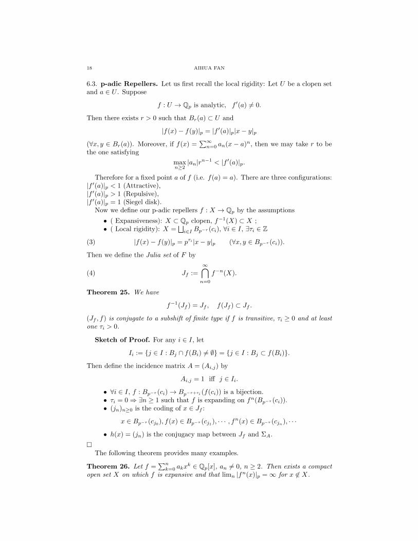
6.3. p-adic Repellers. Let us first recall the local rigidity: Let U be a clopen setand a ∈ U . Suppose

f : U → Qp is analytic, f ′(a) 6= 0.

Then there exists r > 0 such that Br(a) ⊂ U and

|f(x)− f(y)|p = |f ′(a)|p|x− y|p

(∀x, y ∈ Br(a)). Moreover, if f(x) =∑∞n=0 an(x − a)n, then we may take r to be

the one satisfying

maxn≥2|an|rn−1 < |f ′(a)|p.

Therefore for a fixed point a of f (i.e. f(a) = a). There are three configurations:|f ′(a)|p < 1 (Attractive),|f ′(a)|p > 1 (Repulsive),|f ′(a)|p = 1 (Siegel disk).

Now we define our p-adic repellers f : X → Qp by the assumptions

• ( Expansiveness): X ⊂ Qp clopen, f−1(X) ⊂ X ;• ( Local rigidity): X =

⊔i∈I Bp−τ (ci), ∀i ∈ I, ∃τi ∈ Z

(3) |f(x)− f(y)|p = pτi |x− y|p (∀x, y ∈ Bp−τ (ci)).

Then we define the Julia set of F by

(4) Jf :=

∞⋂n=0

f−n(X).

Theorem 25. We have

f−1(Jf ) = Jf , f(Jf ) ⊂ Jf .

(Jf , f) is conjugate to a subshift of finite type if f is transitive, τi ≥ 0 and at leastone τi > 0.

Sketch of Proof. For any i ∈ I, let

Ii := {j ∈ I : Bj ∩ f(Bi) 6= ∅} = {j ∈ I : Bj ⊂ f(Bi)}.

Then define the incidence matrix A = (Ai,j) by

Ai,j = 1 iff j ∈ Ii.

• ∀i ∈ I, f : Bp−τ (ci)→ Bp−τ+τi (f(ci)) is a bijection.• τi = 0⇒ ∃n ≥ 1 such that f is expanding on fn(Bp−τ (ci)).• (jn)n≥0 is the coding of x ∈ Jf :

x ∈ Bp−τ (cj0), f(x) ∈ Bp−τ (cj1), · · · , fn(x) ∈ Bp−τ (cjn), · · ·

• h(x) = (jn) is the conjugacy map between Jf and ΣA.

�The following theorem provides many examples.

Theorem 26. Let f =∑nk=0 akx

k ∈ Qp[x], an 6= 0, n ≥ 2. Then exists a compactopen set X on which f is expansive and that limn |fn(x)|p =∞ for x 6∈ X.

P-ADIC POLYNOMIAL DYNAMICS 19

Sketch of Proof. ∃` (so sufficiently large |x|n−1p |an| ≥ p) such that if |x|p ≥ p`

we have

|f(x)| = |xn|p∣∣∣an +

an−1

x+ · · ·+ a0

xn

∣∣∣ = |xn|p|an| = |x|n−1p |an| · |x|p ≥ p|x|p

by the ultra-metric property

|x+ y|p ≤ max{|x|p, |y|p}.

Let X = Bp`(0). �Remark that We should make the assumption: f ′(x) 6= 0 on X. Then f will

have the rigidity property on X.

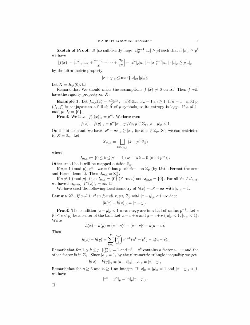
Example 1. Let fm,a(x) = xp−axpm , a ∈ Zp, |a|p = 1,m ≥ 1. If a = 1 mod p,

(Jf , f) is conjugate to a full shift of p symbols, so its entropy is log p. If a 6= 1mod p, Jf = {0}.

Proof. We have |f ′m(x)|p = pm. We have even

|f(x)− f(y)|p = pm|x− y|p∀x, y ∈ Zp, |x− y|p < 1.

On the other hand, we have |xp − ax|p ≥ |x|p for al x 6∈ Zp. So, we can restrictedto X = Zp. Let

Xm,a =⊔

k∈Im,a

(k + pmZp)

where

Im,a := {0 ≤ k ≤ pm − 1 : kp − ak ≡ 0 (mod pm)}.Other small balls will be mapped outside Zp.

If a = 1 (mod p), xp − ax = 0 has p solutions on Zp (by Little Fermat theoremand Hensel lemma). Then Jm,a ' Σ+

p .If a 6= 1 (mod p), then Im,a = {0} (Fermat) and Jm,a = {0}. For all ∀x 6∈ Jm,a,

we have limn→∞ |fn(x)|p =∞. �We have used the following local isometry of h(x) = xp − ax with |a|p = 1.

Lemma 27. If a 6= 1, then for all x, y ∈ Zp with |x− y|p < 1 we have

|h(x)− h(y)|p = |x− y|p.

Proof. The condition |x− y|p < 1 means x, y are in a ball of radius p−1. Let c(0 ≤ c < p) be a center of the ball. Let x = c+u and y = c+ v (|u|p < 1, |v|p < 1).Write

h(x)− h(y) = (c+ u)p − (c+ v)p − a(u− v).

Then

h(x)− h(y) =

p∑k=1

(p

k

)cn−k(uk − vk)− a(u− v).

Remark that for 1 ≤ k ≤ p, |(pk

)|p = 1 and uk − vk contains a factor u− v and the

other factor is in Zp. Since |a|p = 1, by the ultrametric triangle inequality we get

|h(x)− h(y)|p = |u− v|p| − a|p = |x− y|p.

Remark that for p ≥ 3 and n ≥ 1 an integer. If |x|p = |y|p = 1 and |x − y|p < 1,we have

|xn − yn|p = |n|p|x− p|p.�

20 AIHUA FAN

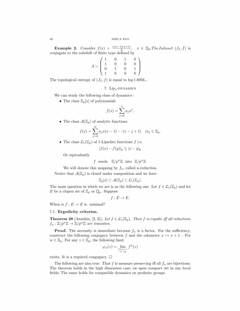
Example 2. Consider f(x) = x(x−1)(x+1)2 , x ∈ Q2.TheJuliaset (Jf , f) is

conjugate to the subshift of finite type defined by

A =

1 0 1 01 0 0 00 1 0 11 0 0 0

The topological entropy of (Jf , f) is equal to log 1.6956...

7. Lip1-dynamics

We can study the following class of dynamics :

• The class Zp[x] of polynomials

f(x) =

n∑j=0

ajxj .

• The class A(Zp) of analytic functions

f(x) =

∞∑j=0

ajx(x− 1) · · · (x− j + 1) (aj ∈ Zp.

• The class L1(Zp) of 1-Lipschtz functions f i.e.

|f(x)− f(y)|p ≤ |x− y|pOr equivalently

f sends Z/pnZ into Z/pnZ.We will denote this mapping by fn, called n-reduction.

Notice that A(Zp) is closed under composition and we have

Zp[x] ⊂ A(Zp) ⊂ L1(Zp).The main question in which we are is as the following one. Let f ∈ L1(Zp) and letE be a clopen set of Zp or Qp. Suppose

f : E → E.

When is f : E → E is minimal?

7.1. Ergodicity criterion.

Theorem 28 (Anashin, [2, 3]). Let f ∈ L1(Zp). Then f is ergodic iff all reductionsfn : Z/pnZ→ Z/pnZ are transitive.

Proof. The necessity is immediate because fn is a factor. For the sufficiency,construct the following conjugacy between f and the odometer x 7→ x + 1 : Fixw ∈ Zp. For any z ∈ Zp, the following limit

ϕw(z) = limZ3n→zin Zp

fn(z)

exists. It is a required congugacy. �

The following are also true. That f is measure preserving iff all fn are bijections;The theorem holds in the high dimension case, on open compact set in any localfields; The same holds for compatible dynamics on profinite groups.

P-ADIC POLYNOMIAL DYNAMICS 21

7.2. Behavior on Zp of a general polynomial. The behavior on Zp of an ar-bitrary polynomial from Zp[x] is clear, due to the following result. The notion ofminimal decomposition reflects the common feature of integer-valued polynomialdynamics.

Theorem 29 (Fan-Liao, [17]). Let f ∈ Zp[x] be a polynomial. We have the follow-ing minimal decomposition

Zp = A tB t C• A: the finite set of all periodic points• B: at most countable union of minimal sets• C: every point of C is attracted by A or B.

This result is generalized to other analytic dynamics and rational dynamics [21,18].

7.3. Minimality on Zp.

Theorem 30 (Anashin [3]). Let f(x) =∑∞k=0 ak

(xk

)be a 1-Lip mapping on Z2.

The dynamics (Zp, f) is minimal iff the following conditions hold simultaneously:

• a0 6≡ 0 (mod 2);• a1 ≡ 1 (mod 4),• ak ≡ 0 (mod 2blog2(i+1)c+1), (k ≥ 2)

Similar conditions are sufficient for p ≥ 3, but not necessary (Anashin). The Re-sult for polynomials (p = 2) using Taylor coefficients is due to Larin (1995). Durandand Paccaut ([15]) obtained a necessary and sufficient condition for polynomials inZ3 to be minimal, using Taylor coefficients.

Theorem 31 (Larin [34]). Let f(x) =∑akx

k ∈ Z2[x]. Then (Z2, f) is minimaliff

(1) a0 ≡ 1 (mod 2);(2) a1 ≡ 1 (mod 2);(3) 2a2 ≡ a3 + a5 + · · · (mod 4);(4) a2 + a1 − 1 ≡ a4 + a6 + · · · (mod 4).

Durand-Paccaut’s result on Z3 is similarly stated.For general quadratic polynomial on any Zp, there is a complete characterization

(Larin, Knuth).

Theorem 32 (Larin [34], Knuth [33]). Let f(x) = ax2 + bx + c with a, b, c ∈ Zp.Then f is minimal iff

(1) When p ≥ 5,

a = 0( mod p), b = 1( mod p), c 6= 0( mod p).

(2) When p = 3,

a = 0( mod 32), b = 1( mod 3), c 6= 0( mod 3)

or

ac = 6( mod 32), b = 1( mod 3), c 6= 0( mod 3).

(3) When p = 2,

a = 0( mod 2), a+ b = 1( mod 4), c 6= 0( mod 2).

22 AIHUA FAN

7.4. Affine dynamics. Affine maps are of the form

Ta,bx = ax+ b (a, b ∈ Qp).Assume a, b ∈ Zp. We get a dynamics (Zp, Ta,b).

Theorem 33 (Fan-Li-Yao-Zhou, [16]). Suppose a, b ∈ Zp and p ≥ 3.

(1) Ta,b is ergodic on Zp iff

a = 1 ( mod p), b 6= 0 ( mod p).

(2) The space Zp is decomposed into at most countable components, restrictedon each of which Ta,b is uniquely ergodic.

Proof. We give a short proof of (1), which is very specific to affine dynamics.Necessity. Since bZp is T is Ta,b-invariant ( for a(bx) + b = b(ax+ 1)), we must

have |b|p = 1. If a 6≡ 1 ( mod p), a − 1 would be invertible and then Ta,b admits afixed point (a− 1)−1b, contradiction.

Sufficiency. Assume |b|p = 1. Then Ta,b is conjugate to Ta,1:

Tb,0 ◦ Ta,1(x) = b(ax+ 1) = a(bx) + b = Ta,b ◦ Tb,0.We can assume that b = 1. Write Ta = Ta,1. Define

Φa(z) :=az − 1

a− 1=

Exp(zLog(a))− 1

a− 1, Ψa(z) :=

Log(1 + (a− 1)z)

Log(a).

which are homeomorphisms from Zp onto Zp and one is the inverse of the other (to check). They realize a congugacy between Ta and T1 ( odometer):

Ta(Φa(z)) = aaz − 1

a− 1+ 1 =

az+1 − 1

a− 1= Φa(z + 1) = Φa(T1(z)).

�We finish by making some remarks:

• The theorem holds for p = 2, but the condition a = 1 ( mod p) must bereplaced by a = 1 ( mod 22).• The multiplication ax was studied by Coelho and Parry.• Another proof uses Fourier series ( [16]): Solutions of f(Ta,b(x)) = f(x) are

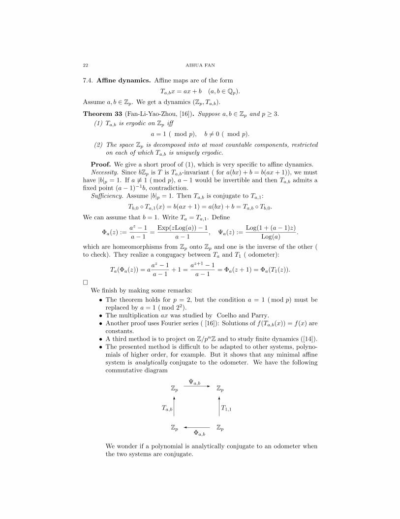
constants.• A third method is to project on Z/pnZ and to study finite dynamics ([14]).• The presented method is difficult to be adapted to other systems, polyno-

mials of higher order, for example. But it shows that any minimal affinesystem is analytically conjugate to the odometer. We have the followingcommutative diagram

Zp- Zp

Ψa,b

6Ta,b

6T1,1

Zp Zp�Φa,b

We wonder if a polynomial is analytically conjugate to an odometer whenthe two systems are conjugate.

P-ADIC POLYNOMIAL DYNAMICS 23

References

[1] V. S. Anashin, Uniformly distributed sequences of p-adic integers, Diskret. Mat., 14 (2002)3–64; translation in Discrete Math. Appl., 12 (6) (2002), 527–590.

[2] V. S. Anashin, Uniformly distributed sequences of p-adic integers, II, Available at

http://arXiv.org/math.NT/0209407.[3] V. S. Anashin, Ergodic transformations in the space of p-adic integers, in p-adic mathematical

physics ed. A. Y. Khrennikov, Z. Rakic and I. V. Volovich, AIP Conference Proceedings vol.

826, 2006, 3–24.[4] V. S. Anashin and A. Khrennikov, Applied Algebraic Dynamics, de Gruyter Expositions in

Mathematics. 49. Walter de Gruyter & Co., Berlin, 2009.[5] D. K. Arrowsmith and F. Vivaldi, Some p-adic representations of the Smale horseshoe, Phys.

Lett. A, 176 (1993), 292294.

[6] D. K. Arrowsmith and F. Vivaldi, Geometry of p-adic Siegel discs, Physica D, 71 (1994),222236.

[7] M. Bhargava, P -orderings and polynomial functions on arbitrary subsets of Dedekind rings,

J. Reine Angew. Math., 490 (1997), 101–127.[8] M. Bhargava, The factorial function and generalizations, Amer. Math. Monthly, 107 (2000),

783–799.

[9] R. Benedetto, Fatou components in p-adic dynamics, PhD thesis, Brown University, 1998.[10] P. J. Cahen and J. L. Chabert, Integer-valued polynomials, Mathematical Survey and Mono-

graphs, vol. 48, American Mathematical Society, Providence, 1997.

[11] J. L. Chabert, A. H. Fan and Y. Fares, Minimal dynamical systems on a discrete valuationdomain, DCDS, 2009.

[12] A. Chambert-Loir, Mesures et equidistribution sur les espaces de Berkovich, J. Reine Angew.Math., 595 (2006), 215–235.

[13] Z. Coelho and W. Parry, Ergodicity of p-adic multiplications and the distribution of Fibonacci

numbers, in Topology, Ergodic Theory, Real Algebraic Geometry, Amer. Math. Soc. Transl.Ser. 2, no. 202, American Mathematical Society, Providence, (2001), 51–70.

[14] D. L. Desjardins and M. E. Zieve, On the structure of polynomial mappings modulo an odd

prime power, Available at http://arXiv.org/math.NT/0103046, 2001.[15] F. Durand and F. Paccaut, Minimal polynomial dynamics on the set of 3-adic integers, Bull.

Lond. Math. Soc., 41(2):302–314, 2009.

[16] A. H. Fan, M. T. Li, J. Y. Yao and D. Zhou, Strict ergodicity of affine p-adic dynamicalsystems on Zp, Adv. Math., 214 (2007), 666-700. See also A. H. Fan, M. T. Li, J. Y. Yao et

D. Zhou, p-adic affine dynamical systems and applications, C. R. Acad. Sci. Paris, Ser. I 342

(2006), 129–134.[17] A. H. Fan and L. M. Liao, On minimal decomposition of p-adic polynomial dynamical systems,

Adv. Math., 228:2116–2144, 2011.

[18] On minimal decomposition of p-adic rational functions with good reduction, preprint 2015.[19] A.H. Fan, S. L. Fan, L. M. Liao, and Y. F. Wang, On minimal decomposition of p-adic

homographic dynamical systems, Adv. Math., 257:92–135, 2014.[20] A. H. Fan, L. M. Liao, Y. F. Wang and D. Zhou, p-adic repellers in Qp are subshifts of finite

type , C. R. Acad. Sci. Paris, 344 (4) (2007), 219–224.[21] S. L. Fan and L. M. Liao, Dynamics of convergent power series on the integral ring of a finite

extension of Qp, J. Differential Equations, 259(4):1628–1648, 2015.

[22] S. L. Fan and L. M. Liao, Dynamics of the square mapping on the ring of p-adic integers, To

appear in Pro. American Math. Society, 2015.[23] C. Favre and J. Rivera-Letelier, Theoreme d’equidistribution de Brolin en dynamique p-

adique, C. R. Math. Acad. Sci. Paris, 339 (4) (2004), 271–276.

[24] C. Favre and J. Rivera-Letelier, Equidistribution quantitative des points de petite hauteursur la droite projective, Math. Ann., 335 (2) (2006), 311–361.

[25] M. Gundlach, A. Khrennikov and K.-O. Lindahl, On ergodic behavior of p-adic dynamicalsystems, Infin. Dimens. Anal. Quantum Probab. Relat. Top., 4 (2001), 569–577.

[26] M. R. Herman and J. C. Yoccoz, Generalization of some theorem of small divisors to non-archimedean fields. In: Geometric Dynamics, LNM 1007, Springer-Verlag (1983), 408-447.

[27] L. Hsia, Closure of periodic points over a non-Archimedean field, J. London Math. Soc., 62

(3)(2000), 685–700.

24 AIHUA FAN

[28] R. Jones, Galois Martingales and the hyperbolic subset of the p-adic Mandelbrot set, PhD

thesis, Brown University, 2005.

[29] Y. Katznelson, Ergodic automorphisms of Tn are Bernoulli shifts, Israel J. Math., 10 (1971),186–195.

[30] A. Khrennikov, Non-Archimedean Analysis: Quantum Paradoxes, Dynamical Systems and

Biological Models, Kluwer, Dordrecht, 1997.[31] A. Khrennikov and M. Nilsson, On the number of cycles of p-adic dynamical systems, J.

Number Th., 90 (2) (2001), 255–264.

[32] A. Yu. Khrennikov and M. Nilsson, p-adic deterministic and random dynamics, Kluver Aca-demic Publ., Dordrecht, 2004.

[33] D. Knuth, The art of computer programming, vol. 2, Seminumerical algorithms, Addison-

Wesley, Third edition, 1998.[34] M. V. Larin, Transitive polynomial transformations of residue class rings, Discrete Mathe-

matics and Applications, 12(2) (2002), 141–154.[35] H. C. Li, p-adic dynamical systems and formal groups, Compositio Math., 104, no. 1 (1996),

41–54.

[36] D. A. Lind, The structure of skew products with ergodic group automorphisms, Israel J.Math., 28 (3) (1977), 205–248.

[37] D. Lind and K. Schmidt, Bernoullicity of solenoidal automorphisms and global fields, Israel

J. Math., 87 no. 1-3 (1994), 33–35.[38] D. A. Lind and T. Ward, Automorphisms of solenoids and p-adic entropy, Erg. Th. Dynam.

Syst., 8(3) (1988), 411-419.

[39] K-O. Lindahl, On Siegel’s linearization theorem for fields of prime characteristic, Nonlinearity,17 (2004), 745-763.

[40] J. Lubin, Non-Archimedean dynamical systems, Compositio Mathematica, 94 (1994), 321–

346.[41] J. M. Luck, P. Moussa and M. Waldschmidt (editors), Number theory and physics, No 47 in

Springer Proceeding in Physics, Berlin, Springer-Verlag, 1990.[42] K. Mahler, p-adic Numbers and their Functions, Cambridge Tracts in Mathematics, vol. 76.,

Cambridge University Press, 1980.

[43] P. Morton and J. Silverman, Periodic points, multiplicities and dynamical units, J. ReineAngew. Math., 461 (1995), 81–122.

[44] R. Oselies and H. Zieschang, Ergodische Eigenschaften der Automorphismen p-adischer

Zahlen, Arch. Math., 26 (1975), 144–153.[45] T. Pezda, Polynomial cycles in certain local domains, Acta Arithmetica, vol. LXVI (1994),

11–22.

[46] J. Rivera-Letelier, Dynamique des fonctions rationnelles sur des corps locaux, Geometricmethods in dynamics. II. Asterisque No. 287 (2003), xv, 147–230.

[47] A. M. Robert, A course in p-adic analysis, Graduate Texts in Mathematics 198, Springer-

Verlag, New York, 2000.[48] W. H. Schikhof, Ultrametric calculus, Cambridge University Press, 1984.

[49] J. Silverman, The Arithmetic of Dynamical Systems, Springer-Verlag, 2007.

[50] V. S. Vladimirov, I. V. Volovich, and E. I. Zelenov, p-adic Analysis and Mathematical Physics,Series on Soviet and East European Mathematics, Vol. 1, World Scientific Co., Inc. 1994.

[51] C. F. Woodcock and N. P. Smart, p-adic chaos and random number generation, ExperimentMath., (1998), 333–342.

Laboratoire Amienois de Mathematiques Fondamentales et Appliquees, CNRS-UMR

7352, Universite de Picardie Jules Verne, 33 rue Saint Leu, 80039 Amiens cedex 1,

France.E-mail address: ai-hua.fan@u-picardie.fr