Introducing the EquiPop software

an application for the calculation of

k-nearest neighbour contexts/neighbourhoods

John Östh

Uppsala University, Department of Social and Economic Geography, Box 513,

SE-751 20 Uppsala (Sweden); email: john.osth@kultgeog.uu.se

Keywords: KNN, k-nearest neighbour, EquiPop, context, contextual analysis,

distance decay, individualised neighbourhood, Egocentric neighbourhood,

bespoke neighbourhood

Abstract

In health science and social science much attention is paid to understand the links between the

contexts in which individuals reside, and the effects these contexts have on peoples choices,

health and similar. Contextual statistics are often derived from area based aggregates or

floating catchment area aggregates and in almost all cases, these aggregates are based on

varying population counts. Depending on research question, population distribution and

shapes of areas or sizes of radiuses, contextual variables with varying population counts may

be more or less reliable in analyses. Using a k-nearest neighbour approach, fixed population

counts may be used to construct contextual variables. Traditionally, non-heuristic, k-nearest

neighbour analyses are computationally very demanding, a fact that has contributed to its

limited use in research. In this article, EquiPop, a software application for the creation of k-

nearest neighbour contexts is presented. EquiPop approaches the k-nearest neighbour

computation using new calculation techniques, which enables the creation of contextual

variables also for spatially very large and detailed datasets in relatively short time spans. How

to install, prepare files, load and run the software, do optional settings as well as handling of

output is presented in this paper.

1. The nature of neighbourhoods and the measurement of contexts

Within health science and social science, the study of contexts and contextual effects usually

centres on individuals and usually using the word “neighbourhood” to capture the individual

contexts, and neighbourhood effects to capture how individuals affect and are being affected

by social networks, topography and extents of a certain area. However, the interchangeable

use of the phrase neighbourhood meaning context is not entirely unproblematic, since

neighbourhoods often are single concepts, representing a piece of territory having little or no

correspondence with human behaviour (Lee, 1968; Galster, 2001). The ‘real’, human-centred

neighbourhoods are more complex and require more than a designated piece of land to be

studied. So complex in fact that bounding a neighbourhood spatially becomes impossible

since different neighbourhood attributes have different and varying scales.

The complexity of neighbourhood means that measuring neighbourhoods becomes difficult.

A pragmatic solution to the measurement problems outlined above is to measure the different

neighbourhood attributes, rather than neighbourhoods, using scales and shapes that suite the

attribute best. This means either using statistics aggregated to some kind of pre-existing areal

unit, using statistics collected using radiuses or using a k-nearest neighbour approach.

Evidently, choosing neighbourhood measurement method becomes important.

There is a large body of work discussing neighbourhoods and especially neighbourhood

effects in both social and health sciences (for review articles see for instance: Pickett & Pearl,

2001; Sampson et al., 2002; Mair et al. 2008; Sellström & Bremberg, 2006). Central in most

of the reviewed articles is that how neighbourhoods are perceived spatially and analytically is

critical for both outcome and inference. There are examples of studies where individual-

centred k-nearest neighbour approaches or bespoke neighbourhoods have been used in social

science and health science (see for instance Johnston et al. 2004, Johnston et al. 2005, Chaix,

et al. 2005 & Davies and Hazelton, 2010). However, as the above listed review articles also

note, contextual or neighbourhood variables are occasionally depicted by fixed bandwidths

(radiuses), almost always represented by fixed area entities such as wards, tracts, blocks or

counties but almost never represented by k-nearest neighbour contexts.

Whether this is a problem or not is entirely dependent on the studied neighbourhood

attribute(s) and the research question at hand. In cases where the area itself contains attributes,

structures or values that define neighbourhood, neighbourhoods are best defined by fixed

border areas. However, for the study of social processes, fixed border areas are problematic

(Sampson et al., 2002). Fixed border areas also disregards the scale and distribution of what is

measured since, leading to biases related to MAUP ( Modifiable Areal Unit Problem) (see for

instance Openshaw, 1994; Wong, 2004; Andersson and Musterd, 2010).

In cases where a predefined radius best depicts the spatial perimeter of the neighbourhood,

radii-based neighbourhoods should be used. This would potentially be more common where

space is an important determinants for the definition of neighbourhoods, such as locations

with proximity to services, scenic views, metro stations or similar. Radii-based

neighbourhoods have been used extensively in planning over a long time where planning

ideals have been centred on reaching local amenities with a short walking distance; see for

instance (Perry 1929/1998). Though a majority of the radii based neighbourhood studies have

been focused on the planned landscape rather than on people, also social processes such as

segregation have successfully been studied using radii-based approaches (Reardon et al.,

2008).

If the spatial relationship between individuals and their ilk (or opposite) define

neighbourhoods, contexts would preferably be defined by the composition of neighbours. This

is preferably done using a k-nearest neighbour approach. That is, as long as the physical

separation between neighbours is not too big for neighbourhoods to be factual.

There is no single good scale or method for the measurement of all attributes taking place

within a neighbourhood since neighbourhood attributes are produced and consumed at

different scales (Galster, 2001). For the measurement of neighbourhood and neighbourhood

effects this means that the palette of methods is best if varied and sensitive to the spatial

structures and scales at play. This also means that the introduction of EquiPop and its method

for the calculation of k-nearest neighbours is to be viewed as a new tool in the toolbox,

specifically designed for easy calculation of k-nearest neighbour statistics also using very

large datasets.

The remainder of the article is focused on the functionality and use of EquiPop. First, the

computational idea behind EquiPop is presented, followed by an installation guide, manual

for running EquiPop and handling its output. Finally two examples of how EquiPop can be

used are presented followed by a conclusion. Additional EquiPop-related material is available

on http://equipop.kultgeog.uu.se.

2. Idea behind EquiPop

Regular non-heuristic k-nearest neighbour computations are very computer demanding. This

because finding the k-nearest neighbour requires all populated locations j to be sorted

adjacently according to their distance from any origin i. By accumulating population counts

from the vector of j until value k has been reached, neighbour and neighbourhood statistics

can be constructed for location i. However, for all other locations i, the sorting and

accumulative counting process needs to be repeated. In cases where the count of locations

reaches thousands or even millions of unique locations, iterative sorting procedures are no

longer viable computation procedures. More pragmatic solutions to the computational

problems are usually to substitute the non-heuristic k-NN algorithms for context

approximations, where fixed-border areas such as municipalities, blocks or wards or floating

catchment areas of a predefined radius are used instead.

In cases where contexts best is studied and understood in terms of neighbouring members of

the studied population, a k-nearest neighbour approach is to prefer. In order to make k-NN

computations possible also in very large datasets, EquiPop calculates k-NN without sorting

the data according to distances between all i and j. Instead, EquiPop categorizes all in-data in

a runtime geocoded matrix according to the x and y coordinates so that the data is arranged

according to their spatial extent. However, the matrix is organized similar to pixels in a digital

image, where space is rectified into gridded units. By gridding the data, calculations of

distances between any units i and j will be less accurate compared to using original

coordinates1. This means that the average error will be more influential on shorter distances

and smaller k-values, since the average error (being fixed) makes up a greater proportion of

the distance.

Using gridded data has a fundamental advantage in the computation of k-nearest neighbours.

From any unit i the distances to surrounding units j will be the same regardless where i is

located (See Östh et al. 2014c). This means that rather than calculating the unique distances

1 On average, the error introduced by gridding will equal roughly 70.7% of the size of the grid-unit

between i and all j:s for each location, a pre-set rule for all distances can be applied. This is

also the single-most important reason why EquiPop can be used to calculate k-NN in larger

datasets.

Currently, EquiPop holds the distance-order instructions for the 4 million nearest units. In

Figure 1 the principle behind gridded distance is shown. From any unit i, the distance to any

unit j, with the suffix “a”, is the same. The same distance relationship is true for all units j

with suffix “b”.

Figure 1 illustrates that the distance between any i and any ja or any i and any jb always will be the same in a gridded dataset.

3. Installation of EquiPop

In order to obtain the software (download from http://equipop.kultgeog.uu.se) the user needs

to enter usage-related information in two steps. First, the user will need to create a user

account online and agree to user-license terms. Secondly, the user needs to enter information

about the computer(s) on which the software is installed. Thereafter the user will be able to

download the software and an activation code.

Two files are available for installation. The EquiPop-file contains the GUI (Graphical User

Interface), from which all EquiPop operations are controlled, while the EquiPop-service-file

contains the computational parts. The separation of the GUI and computational parts enables

users to install computing demanding parts of the software on a fast computer/server, whilst

the GUI-part of the program may be installed on any computer having Windows as OS2. It is

possible to install the EquiPop-file on several computers, all sharing the same EquiPop-

service. EquiPop has been developed in C# using Windows-NET. This means that a .NET

framework needs to be installed on the computer3. During installation of the EquiPop file, the

user will be asked to configure the EquiPop-service endpoint by confirming or adding an

URL for the installed EquiPop-service. By default the address is

http://localhost:19999/equipop, where “localhost” indicates that the computational parts of the

program are located on the same computer as is the GUI. If the user decides to separate GUI

and computational parts, the URL needs to be reformulated so that “localhost” is replaced

with an IP or DNS-address – however, the “:19999/equipop” part should remain unaltered4.

There is no installation order for the EquiPop and EquiPop-service files as long as the service

endpoint URL points to the correct computer. However, after a trial period the user will be

prompted to enter an activation code. The activation code is generated on the EquiPop website

and renders the user access to EquiPop during the 365 days following registration. The

activation code can be updated online after installation.

4. Preparing files for EquiPop

Central for the preparation of EquiPop input files is to determine a ‘good-enough’ grid unit,

fine enough not to compromise local characteristics and spatial patterns but not large enough

to make computing time-consuming. A first step is to determine the minimum distance

between any two objects in the studied population. The ‘Near’ function in ArcGis can be used

to retrieve minimum distances as well as finding out near distances for different percentiles in

the population. Choosing a grid unit smaller than the observed minimum distance will ensure

that data will not need to be aggregated. However, if the dataset is detailed and spans over

larger areas, some aggregation may need to be accepted. In two recent analyses of segregation

in California (Clark et al. 2014; Östh et al. 2014d), a grid unit of 250ft was chosen for the

analysis of the racial composition on block-level. In a few cases, the block-midpoint to block-

midpoint distances were shorter than 250ft. In those cases the block populations were

aggregated and treated as one.

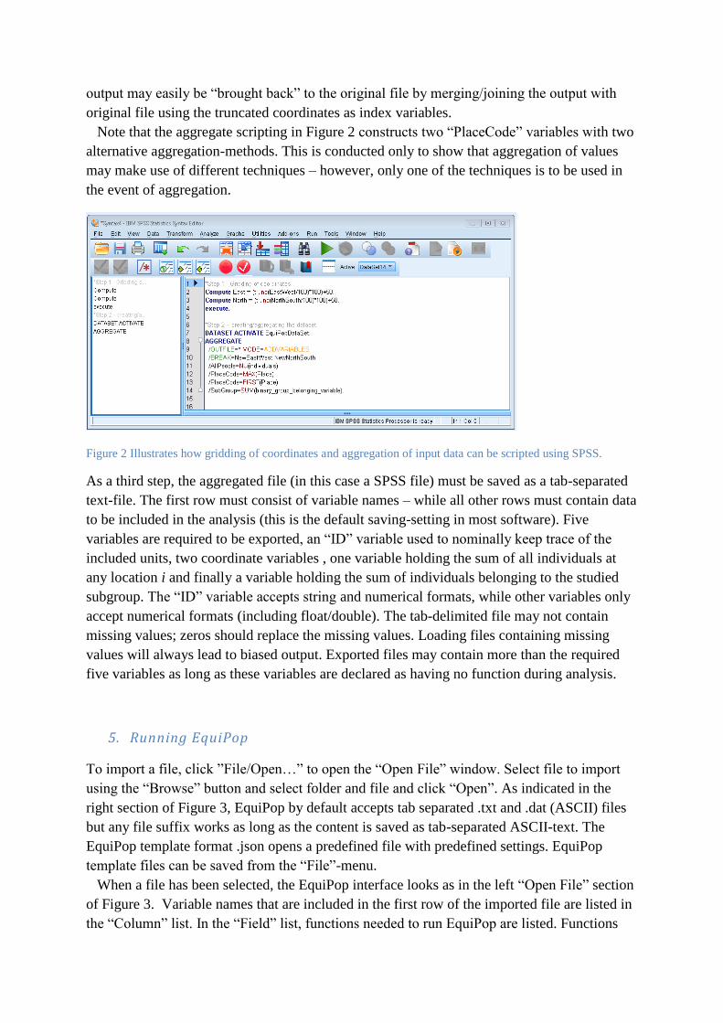
In the second step the data is gridded and aggregated. In Figure 2, an example of how

gridding and aggregation of data is conducted for future use in EquiPop is shown. Where

truncating of coordinates are conducted in the first step and aggregation of an EquiPop dataset

in the second. In the example, SPSS-syntax is used to exemplify – however, most statistics

and/or spreadsheet software can be used. If another software is used the SPSS syntax can be

seen as pseudo-code.

The truncation procedure in the syntax takes out all coordinate details finer than 100 metric

units and aligns/rounds them all to the nearest 50 metric unit. The following aggregation

procedure makes sure that not more than one instance of each pair of coordinates may exist. It

is important not to have coordinate duplicates in the in-data file since the last encountered

value will overwrite any former values (leading to biased output). After running EquiPop, the

2 Tested on Windows Vista/7/ 8 & Windows server 2003/2008/2012 R2

3 .NET can be found on Microsoft.com

4 Number refers to port used for transferring of data between EquiPop and EquiPop-service.

output may easily be “brought back” to the original file by merging/joining the output with

original file using the truncated coordinates as index variables.

Note that the aggregate scripting in Figure 2 constructs two “PlaceCode” variables with two

alternative aggregation-methods. This is conducted only to show that aggregation of values

may make use of different techniques – however, only one of the techniques is to be used in

the event of aggregation.

Figure 2 Illustrates how gridding of coordinates and aggregation of input data can be scripted using SPSS.

As a third step, the aggregated file (in this case a SPSS file) must be saved as a tab-separated

text-file. The first row must consist of variable names – while all other rows must contain data

to be included in the analysis (this is the default saving-setting in most software). Five

variables are required to be exported, an “ID” variable used to nominally keep trace of the

included units, two coordinate variables , one variable holding the sum of all individuals at

any location i and finally a variable holding the sum of individuals belonging to the studied

subgroup. The “ID” variable accepts string and numerical formats, while other variables only

accept numerical formats (including float/double). The tab-delimited file may not contain

missing values; zeros should replace the missing values. Loading files containing missing

values will always lead to biased output. Exported files may contain more than the required

five variables as long as these variables are declared as having no function during analysis.

5. Running EquiPop

To import a file, click ”File/Open…” to open the “Open File” window. Select file to import

using the “Browse” button and select folder and file and click “Open”. As indicated in the

right section of Figure 3, EquiPop by default accepts tab separated .txt and .dat (ASCII) files

but any file suffix works as long as the content is saved as tab-separated ASCII-text. The

EquiPop template format .json opens a predefined file with predefined settings. EquiPop

template files can be saved from the “File”-menu.

When a file has been selected, the EquiPop interface looks as in the left “Open File” section

of Figure 3. Variable names that are included in the first row of the imported file are listed in

the “Column” list. In the “Field” list, functions needed to run EquiPop are listed. Functions

can be dragged from the “Field” list and dropped onto variables in the “Column” list. The

association between function and variables is confirmed in the “Mapped field” list. In case the

imported file contains more than the five variables needed for running EquiPop, the function

“None” needs to be dropped on remaining variables.

At the bottom of the “Open File” interface, users may enter a rectification-unit value. By

default this textbox is empty but in cases where the rectification unit is known to the user, the

value may be entered. If left empty, EquiPop will search the imported data and set the

rectification value automatically. It should be noted that by setting rectification value

incorrectly, computation output will be biased5. By clicking “OK” the file importation settings

are accepted and the main EquiPop interface is shown.

Figure 3 illustrates windows used for importation of files for analysis.

After importation of an analysis file, k-levels need to be set, output-variables to be selected

and decay mode and decay parameter determined before the computations can start. First, the

k-levels need to be set. In Figure 4 requested settings are shown in detail where sections 1a

and 1b illustrate how k-levels are added to and deleted from the running-order list. Requested

value is typed in the top left textbox and added to the running-order list by clicking “Add”

(1a.). By selecting value in the running-order list and by clicking “Delete” the value can be

removed (1b). The running-order list can contain multiple values. Theoretically, there is

neither a maximum count of k-values nor a maximum k-value that can be entered. However,

for each k-level additional sets of output-variables will be created during runtime making

larger datasets with multiple k-levels challenging for some computers. Similarly, very large k-

values mean that very large neighbourhoods need to be searched which in turn will increase

computation time.

If accepting default settings, EquiPop is ready to run at this point. Click the “Run analysis”

button and the analysis will start. During runtime, an approximation of remaining time for

computation will be illustrated by the progress-bar (2 in Figure 4). The progress-bar indicates

time by increasing the green part of the progress-bar until computation is ready. During

runtime it is possible to load and start the next rounds of analysis. Analyses not yet started

will show up in a queue.

Under the running-order list, four checkboxes (checked by default) enables the user to 5 Setting value manually limits computation times marginally. Practical use includes setting finer rectification

units than automatically generated. This is desirable in certain comparative frameworks.

determine which output-variables to save. For each k-level defined by the user, every checked

output-variable will report output-variables for the corresponding k. The “Include distance”

will report the Euclidian distance from each location i to location j where the user defined k-

value was reached. The “Include count all” will report the factual k at every user defined k.

This seemingly odd variable is useful in aggregated datasets. For instance, if the original

dataset consists of individuals whilst the used file is aggregated to block mid-points, the

factual k-value is often a bit greater than the requested user defined value. To exemplify, if the

runtime value < k before adding an additional block but becomes > k after adding the next

nearest block, reported variable value will be based on the count after adding the next nearest

block. Similarly, the two remaining variables “(Include) count group” and “(Include) ratio”

will report factual k-values. The “count group” reports the count of members belonging to the

treatment population for each k and the “ratio” reports the quota of “count group” over “count

all”. When larger datasets with multiple k-levels are studied, either “count all”, “count group”

or “ratio” can be excluded to reduce file-size. The missing variable can easily be calculated in

retrospect.

By default EquiPop runs without distance decay. This means that all objects/individuals will

be assumed to contribute with equal weight to the reported output-variables regardless of

distance from i. In case more distant objects/individuals are assumed to be of less importance,

five different distance decay models including exponential, exponential normal, exponential

square-root, log-normal and power-functions may be employed (see 3a. and 3b. in Figure 4).

The properties of various decay models are discussed at length in the works of Wilson (1981),

Fotheringham and O’Kelly (1989) and Reggiani et al. (2011). For specifications of decay

parameters see for instance Östh et al. (2014a and 2014b)

Figure 4 illustrates how k-levels are defined (1a. and 1b), runtime progression (2) and the specification of

distance decay models.

In the “processing status” section (2 in Figure 4) a completed analysis is identified not only by

the progression of the green progress-bar but also through the file-name that transforms itself

to a HTML-link by which the user can download a zip-file containing the output. Clicking the

link will trigger the default web-browser to open and a transfer of the output from EquiPop to

the computer’s “Downloading area”. It is important to note that the web-browser is used as a

service provider and no data is transferred externally. Having that said, during installation, the

user may choose to separate installations of the computational parts of EquiPop and the GUI.

If the computational parts are installed on another computer data will be transferred over the

Intranet/ Internet.

In the left section of Figure 5 the arrow points at a “downloaded” zip-file ready for

decompression. In the right section of Figure 5, the two files contained by the zip-file are

shown; 1a shows a meta-information-file and 1b the contents of the meta-information file. It

should be noted that the contents of the meta-information file, describing the settings and file

use, is identical to the information shown in the “mouse-cursor-fly-over” message shown

under section 2 in Figure 4. Label 2 in Figure 5 points to the file containing the analysis

output. The output file is always named as the input file.

Figure 5 Illustrates how a zipped folder containing metadata and EquiPop output is saved/downloaded (left) and

what the zipped folder contains (right)

6. Handling EquiPop output

EquiPop output is arranged as tab-separated ASCII. This format guarantees that output can be

opened in many software packages. The output variables can be categorized into three main

groups – files always created, files created for each k if checked during setup and files created

if checked and distance decay is specified. In table 1, variables from an EquiPop run with k-

levels 25 and 50 are illustrated. In the Always category, the first five variables are identical to

the five input variables, however renamed after function. The four remaining variables in the

Always category form a special case. Results are saved to these four variables in cases where

the highest k-value has been reached and EquiPop moves on to the next location i for search

of k-nearest neighbours or when the k-levels are too large (for example greater than the sum

of individuals in the population) and/or the spatial distribution of the studied population

means that some individuals will be located far from others the requested k-level may not be

reached within the four million next nearest gridded units. In order not to be caught in an

(almost) eternal search loop, EquiPop terminates the search for the k-nearest neighbours from

any location i if the requested k has not been reached when four million units have been

searched. Before moving to the next unit the (maximum) count of individuals in the

population is saved to the variable “SumCountAll”, the sum of subgroup members are saved

to “SumCountGroup”, the ratio between “SumCountGroup” over “SumCountAll” is saved to

the “Ratio” variable. Finally, the “MaxDistance” variable describes at what distance from unit

i where the last neighbour was counted before terminating.

If checked, four variables are added for each k-level entered by the user. The four variables

are “IntervalSumCountAll_x”,”IntervalSumCountGroup_x”, “IntervalRatio_x” and

“IntervalDistance_x” where x represents the user entered k-value. Variable

“IntervalSumCountAll_x” holds the factual count of individuals needed to reach k-level “x”

and ”IntervalSumCountGroup_x” holds the equivalent count of treatment group members. In

“IntervalRatio_x” the quota of ”IntervalSumCountGroup_x” over

”IntervalSumCountGroup_x” is calculated and saved. Finally, the “IntervalDistance_x”

variable holds the Euclidian distance between origin location i and the unit where the k=x

nearest neighbour was encountered.

The corresponding decayed variables are making use of the same k-values as the non-

decaying variables6. What is different with this type of variables is that encountered

individuals are given less weight (according to decay specification) as distance increases. This

means that decayed count variables by necessity have smaller values that non-decayed.

Table 1 Variables exported in EquiPop output files. Column “Always” lists variables always being exported,

column “if checked” lists variables being exported if variables are checked during setup. Variables “If checked

plus decay is activated” are exported if variables are checked during setup and distance decay settings are used.

Variables Always if checked If checked plus

decay is activated

Id X

EastWest X

NorthSouth X

CountAllLocal X

CountGroupLocal X

SumCountAll X

SumCountGroup X

Ratio X

MaxDistance X

IntervalSumCountAll_25 X

IntervalSumCountGroup_25 X

IntervalRatio_25 X

IntervalSumCountAllDecay_25 X

IntervalSumCountGroupDecay_25 X

IntervalRatioDecay_25 X

IntervalDistance_25 X

IntervalSumCountAll_50 X

IntervalSumCountGroup_50 X

IntervalRatio_50 X

IntervalSumCountAllDecay_50 X

IntervalSumCountGroupDecay_50 X

IntervalRatioDecay_50 X

IntervalDistance_50 X

6 This is also the reason why no specific distance decay distance variable is available.

Due to the size of the output-files certain third-party software will be needed for the analysis

of the output. Using spreadsheet software, EquiPop-output can be imported to Excel as long

as the file-import format is changed from spreadsheet to text. The importation wizard will

present the user with different alternatives. By choosing “delimited” rather than “fixed width”

as importation method, the tab-separated order of the EquiPop-output file will be used parse

values to cells in the spreadsheet. Importation to statistical software such as SPSS is

conducted in similar fashion7. Many GIS software can transform the EquiPop output files to

shape-files directly in the software. For ArcGis, the file-suffix must be changed to .txt to be

recognized.

7. Two short examples- using EquiPop with a slightly different angle

EquiPop is designed to calculate ratios, i.e. to find out how many from any subpopulation x

that can be found within the k-nearest neighbours from any origin i. This means that all in-

data is arranged as counts where individuals are listed either as belonging to or not belonging

to the studied subgroup in question. Below, two slightly different analyses are conducted.

First, historical epidemical data are used to find out spatial concentrations of incidences in

terms distance needed to encounter 100 cases. Second, by tweaking the input data, EquiPop

can be used to calculate mean values. In the second example, average age for the 6 400

nearest neighbours year 2010 in Sweden is analysed. The purpose of these two examples is to

inspire users to set up analyses also where some data is missing (as in the first example) or

where other results than ratios are preferred (as in the second example).

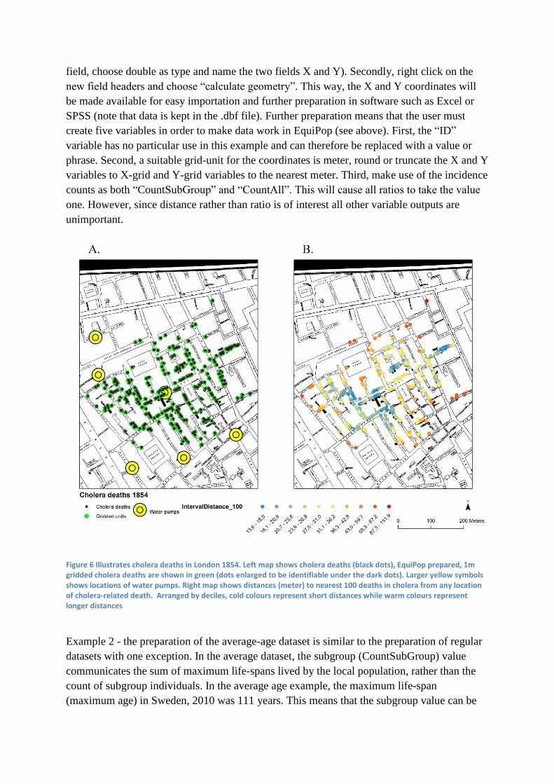
Example 1 - a pioneer in mapping epidemical incidences was John Snow. In 1854, Snow used

a map to show that Cholera deaths in Soho, London, were clustered around a certain water

pump (Johnson, 2006). In this example we make use of EquiPop to calculate distances needed

to reach a k-level of 100 deaths from any location where a cholera-related death was

observed. In Figure 6, the results are revealed. Map B., shows that for almost 20% of the

addresses hit by the epidemic no less than 100 fatalities were encountered within 20 meters

and almost 50% were encountered within 30 meters (deciles were used to categorize the

distances). The spatial relationship between pumps and deaths is illustrated in section A.,

where yellow markers indicate pumps, dark dots indicated addresses where cholera deaths

were encountered and finally, larger green dots indicating the locations of the EquiPop-

gridded units, used in analysis (made larger to be visible).

The data needed for this analysis was downloaded from Robin’s blog (2014). Robin has

kindly digitized incidences and water pumps from Snow’s map and projected the material to

OSGB 1936 / British National Grid, and made it available for public use.

Though the mapped material is made available as a shape-file it is not automatically ready

for use in EquiPop. Using ArcMap as a tool for preparing, this is how the preparation is

conducted. First two fields holding doubles are added (open attribute table and choose add

7 The importation wizard in SPSS sometimes lists the ratio-variables as string-variables rather

than numerical variables – changing the importation format to “dot” solves this problem.

field, choose double as type and name the two fields X and Y). Secondly, right click on the

new field headers and choose “calculate geometry”. This way, the X and Y coordinates will

be made available for easy importation and further preparation in software such as Excel or

SPSS (note that data is kept in the .dbf file). Further preparation means that the user must

create five variables in order to make data work in EquiPop (see above). First, the “ID”

variable has no particular use in this example and can therefore be replaced with a value or

phrase. Second, a suitable grid-unit for the coordinates is meter, round or truncate the X and Y

variables to X-grid and Y-grid variables to the nearest meter. Third, make use of the incidence

counts as both “CountSubGroup” and “CountAll”. This will cause all ratios to take the value

one. However, since distance rather than ratio is of interest all other variable outputs are

unimportant.

Figure 6 Illustrates cholera deaths in London 1854. Left map shows cholera deaths (black dots), EquiPop prepared, 1m gridded cholera deaths are shown in green (dots enlarged to be identifiable under the dark dots). Larger yellow symbols shows locations of water pumps. Right map shows distances (meter) to nearest 100 deaths in cholera from any location of cholera-related death. Arranged by deciles, cold colours represent short distances while warm colours represent longer distances

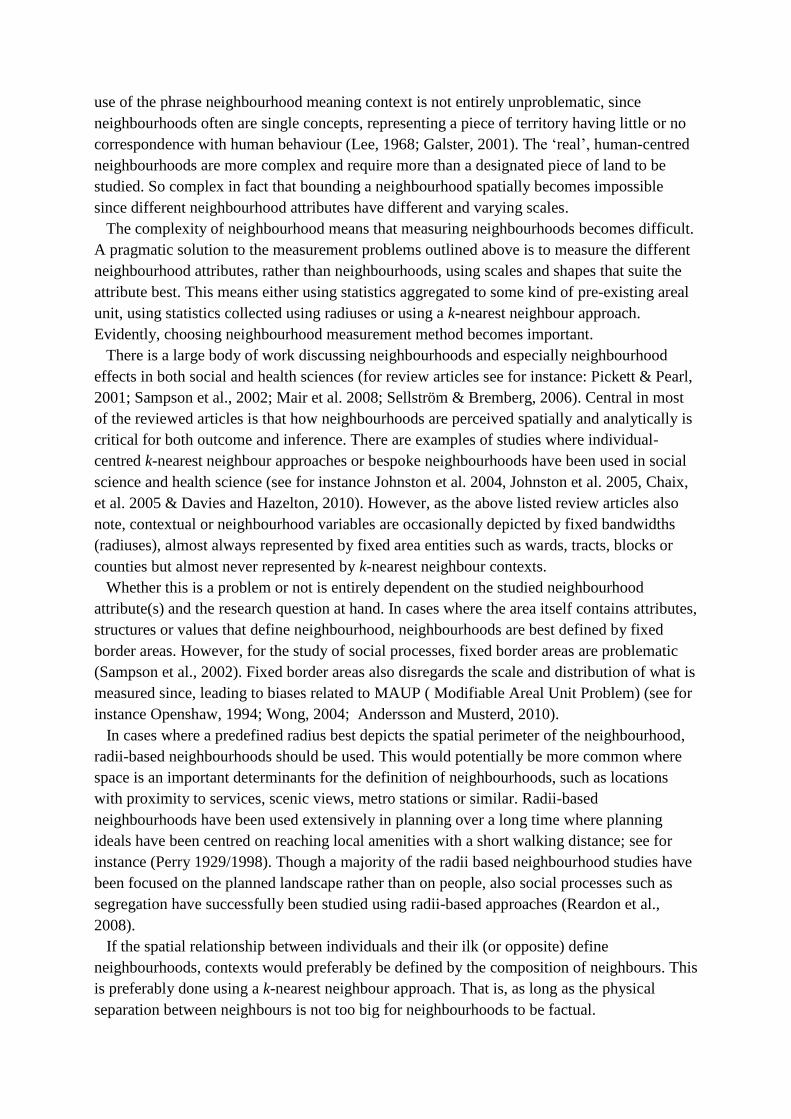
Example 2 - the preparation of the average-age dataset is similar to the preparation of regular

datasets with one exception. In the average dataset, the subgroup (CountSubGroup) value

communicates the sum of maximum life-spans lived by the local population, rather than the

count of subgroup individuals. In the average age example, the maximum life-span

(maximum age) in Sweden, 2010 was 111 years. This means that the subgroup value can be

defined as the sum all years lived by the local residents divided by the maximum age in

Sweden. Since EquiPop accepts decimal values in the variables, the variable should not be

rounded to the nearest integer.

After running the dataset in EquiPop, the ratio-variables should be multiplied with the

maximum age lived to produce the average age among the k-nearest neighbours from any

location i. In Figure 7, the left-side maps are illustrating the average ages in Sweden 2010,

using 2% quantiles. The right-side maps illustrate the average ages using fixed-age-intervals

(0.5 years per colour). The 2x3 top maps magnify average-age patterns in the three major

metropolitan areas. The average-age maps are interesting from two perspectives. First, from a

computational perspective, the analysis make use of almost 800 000 unique, populated

locations and millions of unpopulated spatial units using a grid of 100m x 100m. The

computation-time on a 28 GB RAM, workstation is less than 10 minutes. Secondly, from an

age-distribution perspective, the results show that average age varies considerably between

parts of the country. It is noteworthy that younger individuals are clustered in ‘islands’ around

the major city areas, while rural areas are considerably older.

Figure 7 Illustrates average age among k=6 400 nearest neighbours in Sweden 2010. The left-side maps are illustrating the average ages in Sweden 2010, using 2% quantiles. The right-side maps illustrate the average ages using fixed age-intervals (0.5 years per colour).

8. Conclusion

Using a k-nearest neighbour approach to denote individual centred neighbourhoods can in some

analyses be more accurate than using administrative areas or radii based areas. By introducing the

EquiPop software application, k-nearest neighbour computations can be conducted with greater

ease, also in datasets containing millions of populated locations. This article has demonstrated how

EquiPop is installed, data is prepared, analyses conducted and output used. The demonstration

shows that EquiPop is capable of counting shares of the studied population belonging to any studied

subgroup at any specific k-values and for any location i. In addition, settings or methods for the

calculation of mean values, distances, making use of several k-values at the same time, as well as

enabling for analyses of different distance decay functions are included in the software.

ACKNOWLEDGMENT: The author gratefully acknowledges financial support from VR project 2012-

5509 “Stadens segrationsmönster: En internationell jämförande studie av boendesegregationens

mönster, drivkrafter och effekter”

References

Andersson, R. & Musterd, S., (2010), What scale matters? Exploring the relationships between

individuals’ social position, neighbourhood context and the scale of neighbourhood,

Geografiska Annaler: Series B, Human Geography 92 (1): 23–43.

Chaix, B., Merlo, J., Subramanian, S. V., Lynch, J. and Chauvin, P. (2005): 'Comparison of a Spatial

Perspective with the Multilevel Analytical Approach in Neighborhood Studies: The Case of

Mental and Behavioral Disorders due to Psychoactive Substance Use in Malmö, Sweden, 2001'.

American Journal of Epidemiology, vol, 162 no, 2 pp 171-182.

Clark A. William, Malmberg Bo & Östh John, (PAA 2014), Segregation and De-segregation in

Metropolitan Contexts: Los Angeles as a paradigm for our changing ethnic world.

Davies, T. M. and Hazelton, M. L. (2010): 'Adaptive kernel estimation of spatial relative risk'. Statistics

in Medicine, vol, 29 no, 23 pp 2423-2437.

Fotheringham, A.S. and M.E. O’Kelly (1989), Spatial Interaction Models: Formulations and

Applications, Dordrecht: Kluwer Academic.

Galster George, (2001), On the Nature of Neighbourhood, Urban Studies, Vol. 38, No. 12, 2111–2124

Johnson, Steven (2006), The Ghost Map: The Story of London's Most Terrifying Epidemic – and How it

Changed Science, Cities and the Modern World. Riverhead Books. ISBN 1-59448-925-4

Johnston, R. J., Jones, K., Burgess, S., Propper, C., Sarker, R., & Bolster, A. (2004) Scale, factor

analyses, and neighborhood effects, Geographical Analysis 36(4): 350–369.

Johnston, R. J., Propper, C., Burgess, S., Sarker, R., Bolster, A. & Jones, K., (2005), Spatial scale and the

neighbourhood effect: multinomial models of voting at two recent British general elections,

British Journal of Political Science 35 (3): 487–514

Lee, T., (1968), Urban Neighbourhood as a Socio-Spatial Schema, Human Relations 1968 21: 241,

DOI: 10.1177/001872676802100303

Mair C., Diez Roux, A V. & Galea S., (2008), Are neighbourhood characteristics associated with

depressive symptoms? A review of evidence Journal of Epidemiology and Community Health;

62:940–946. doi:10.1136/jech.2007.066605

Openshaw, S. (1984). The modifiable areal unit problem, CATMOG (Concepts and Techniques in

Modern Geography). Geo Abstracts:40.

Östh John, Clark A. William. & Malmberg Bo, (forthcoming in Geographical Analysis), Measuring the

scale of segregation using k-nearest neighbor aggregates

Östh John, Lyhagen, Johan and Reggiani Aura, (2014b), Half-life and Spatial Interaction Models: Job

Accessibility Analysis in Sweden, Forthcoming in European Journal of Transport and

Infrastructure Research

(online estimator: http://files.kultgeog.uu.se/files/spatialanalysis/halflife.html)

Östh, John, Malmberg, Bo and Andersson, Eva, (2014c) Analysing segregation with individualized

neighbourhoods defined by population size, in C. D. LLOYD, I. SHUTTLEWOTH and D. WONG

(Ed.) Social-Spatial Segregation: Concepts, Processes and Outcomes, Policy Press.

Östh, John, Reggiani, Aura and Galiazzo, Giacomo (2014a) Conventional and New Approaches for the

Estimation of Distance Decay in Potential Accessibility Models: Comparative analyses, in

Condeço Ana, Reggiani Aura & Gutiérrez Javier (Ed.) Accessibility and spatial interaction,

Edward Elgar (EE).

Perry, C., (1929/1998), The Neighbourhood Unit (1929) Reprinted Routledge/Thoemmes, London,

1998

Pickett, K. E., & Pearl, M. (2001), Multilevel analyses of neighbourhood socioeconomic context and

health outcomes: a critical review, J Epidemiol Community Health 2001;55:111–122

Reardon, S. F., S. A. Matthews, D. O'Sullivan, B. A. Lee, G. Firebaugh, C. R. Farrell, and K. Bischoff.

(2008). The geographic scale of metropolitan racial segregation. Demography 45 (3):489-514.

Reggiani, A., P. Bucci, and G. Russo, (2011), ‘Accessibility and impedance forms: empirical

applications to the German commuting networks’, International Regional Science Review 34

(2), pp. 230-252.

Robin’s blog (2014), file: SnowGIS_SHP.zip,

URL: http://blog.rtwilson.com/john-snows-cholera-data-in-more-formats/

Sampson R. J., Morenoff J. D. & Gannon-Rowley T., (2002), Assessing “Neighborhood Effects”: Social

Processes and New Directions in Research, Annual Review of Sociology, Vol. 28, pp. 443-478

Sellström E. & Bremberg S., (2006), The significance of neighbourhood context to child and

adolescent health and well-being: A systematic review of multilevel studies, Scandinavian

Journal of Public Health, 34: 544–554

Wilson, A. G. (1981), Geography and the Environment: Systems Analytical Methods, Chichester: John

Wiley & Sons.

Wong, D. (2004) Comparing traditional and spatial segregation measures: a spatial scale perspective.

Urban Geography 25, 66-82