Introduction (2/2) – Comparison of Modalities

Review:

Modalities:

X-ray: Measures line integrals of attenuation coefficient

CT: Builds images tomographically; i.e. using a set of projections

Nuclear: Radioactive isotope attached to metabolic marker

Strength is functional imaging, as opposed to anatomical

Ultrasound: Measures reflectivity in the body.

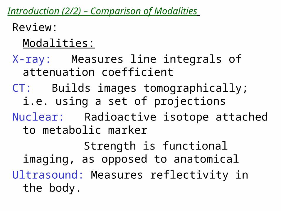
UltrasoundUltrasound uses the transmission and reflection of acoustic energy.

prenatal ultrasound image

clinical ultrasound system

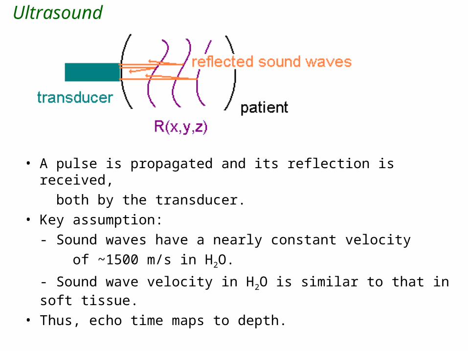
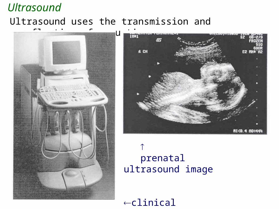
Ultrasound

• A pulse is propagated and its reflection is received,

both by the transducer.

• Key assumption:

- Sound waves have a nearly constant velocity

of ~1500 m/s in H2O.

- Sound wave velocity in H2O is similar to that in soft tissue.

• Thus, echo time maps to depth.

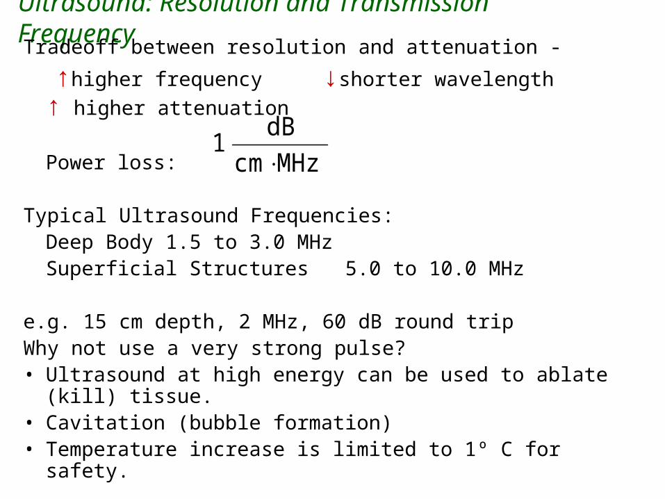
Ultrasound: Resolution and Transmission FrequencyTradeoff between resolution and attenuation -

↑higher frequency ↓shorter wavelength ↑ higher attenuation

Power loss:

Typical Ultrasound Frequencies: Deep Body 1.5 to 3.0 MHzSuperficial Structures 5.0 to 10.0 MHz

e.g. 15 cm depth, 2 MHz, 60 dB round tripWhy not use a very strong pulse?• Ultrasound at high energy can be used to ablate (kill) tissue.• Cavitation (bubble formation)• Temperature increase is limited to 1º C for safety.

MHz cm

dB 1

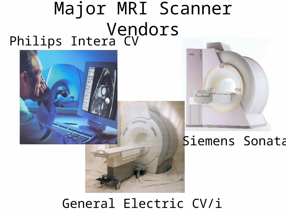
Major MRI Scanner Vendors

Siemens Sonata

General Electric CV/i

Philips Intera CV

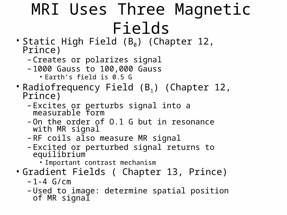
MRI Uses Three Magnetic Fields• Static High Field (B0) (Chapter 12, Prince)

– Creates or polarizes signal– 1000 Gauss to 100,000 Gauss

• Earth’s field is 0.5 G

• Radiofrequency Field (B1) (Chapter 12, Prince)– Excites or perturbs signal into a measurable form– On the order of O.1 G but in resonance with MR

signal– RF coils also measure MR signal– Excited or perturbed signal returns to equilibrium

• Important contrast mechanism

• Gradient Fields ( Chapter 13, Prince)– 1-4 G/cm– Used to image: determine spatial position of MR

signal

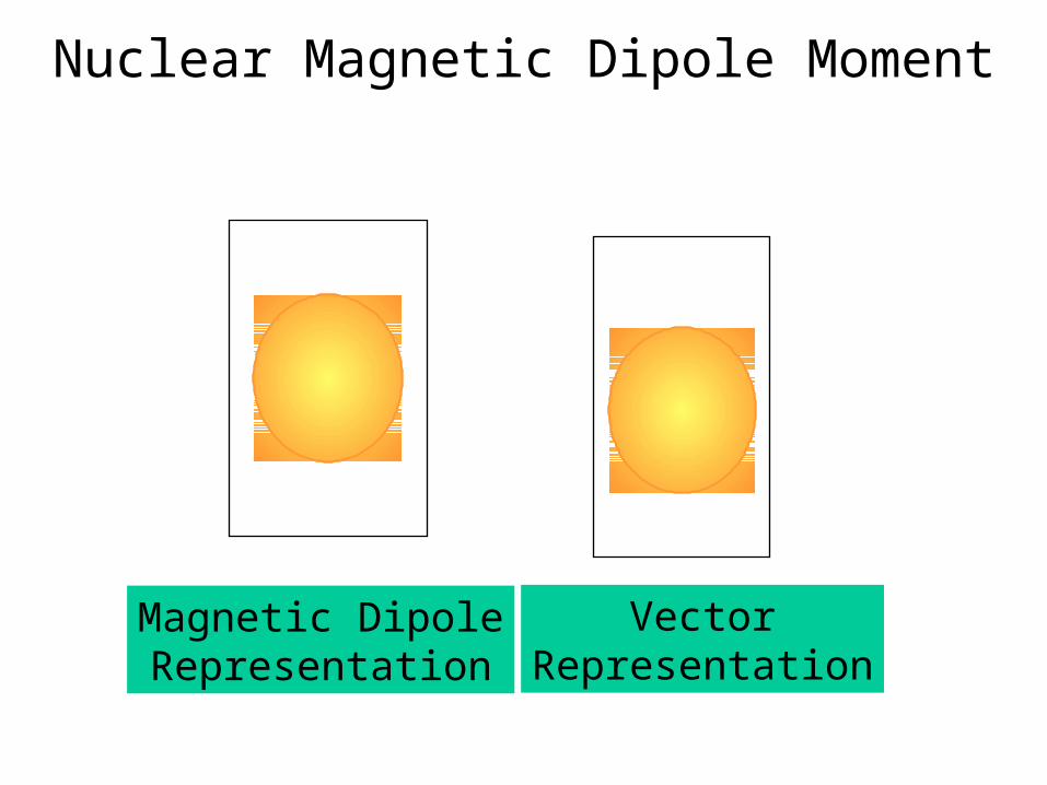
Magnetic DipoleRepresentation

VectorRepresentation

Nuclear Magnetic Dipole Moment

N

S

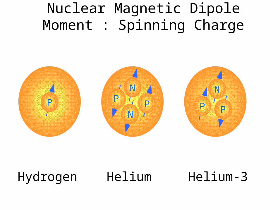
Nuclear Magnetic Dipole Moment : Spinning Charge

P PP

N

NP P

Hydrogen Helium Helium-3

N

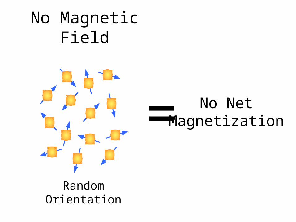
No Magnetic Field

RandomOrientation

= No NetMagnetization

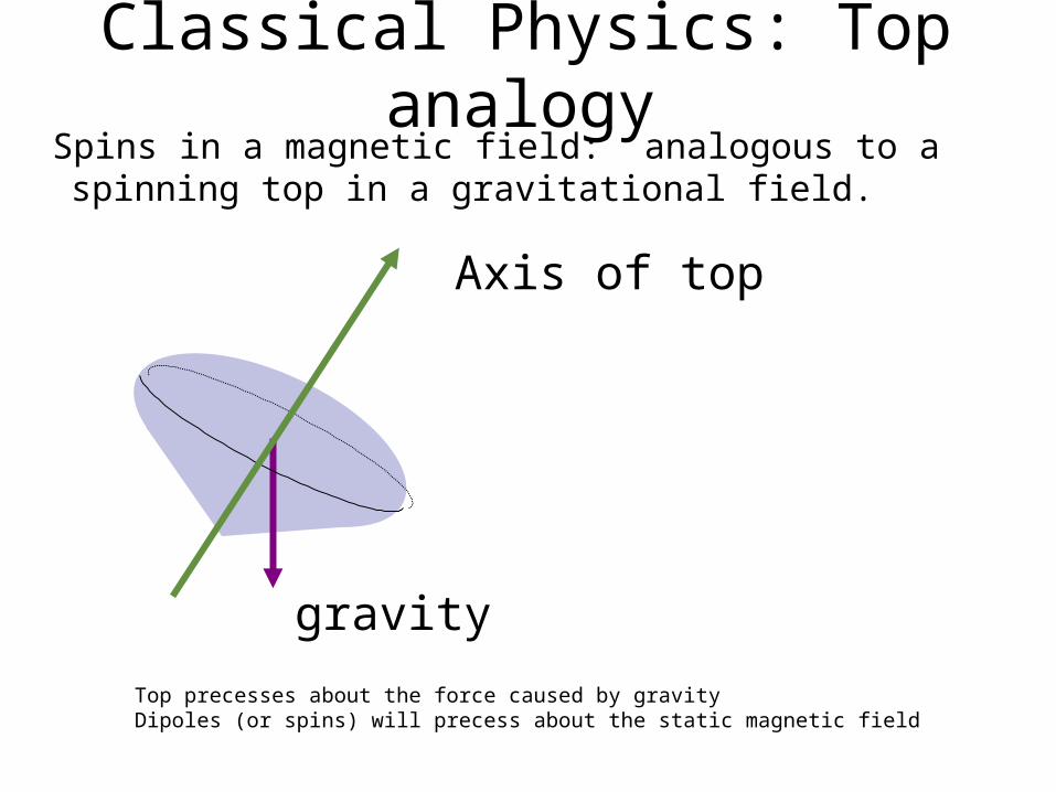
Classical Physics: Top analogy Spins in a magnetic field: analogous to a spinning top in a

gravitational field.

gravity

Top precesses about the force caused by gravityDipoles (or spins) will precess about the static magnetic field

Axis of top

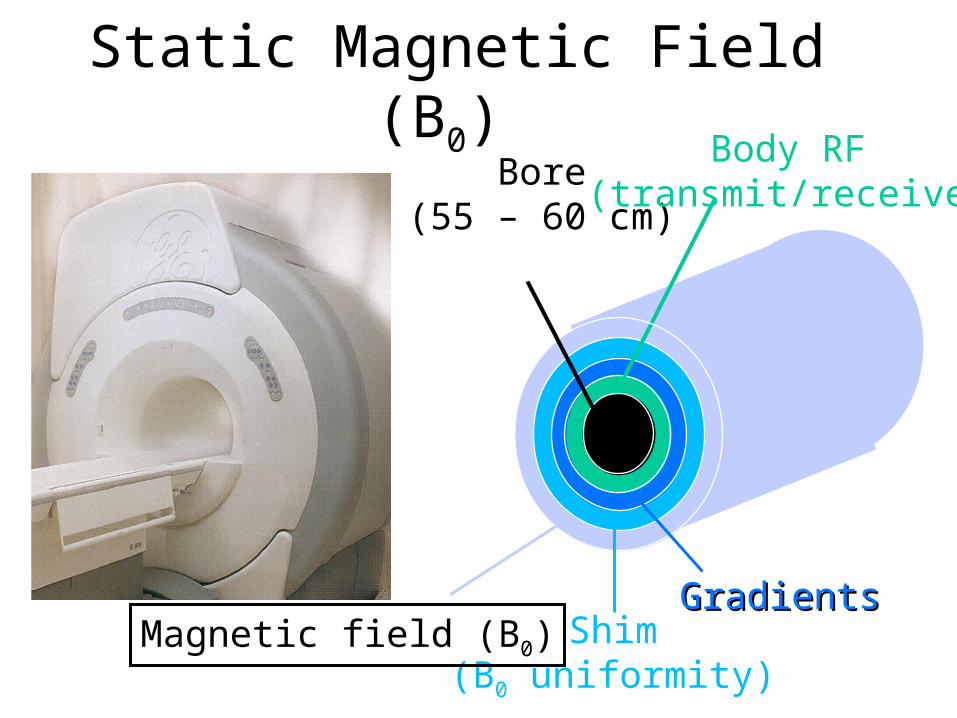
Static Magnetic Field (B0)

Bore(55 – 60 cm)

Shim(B0 uniformity)

Magnetic field (B0)

Body RF(transmit/receive)

GradientsGradients

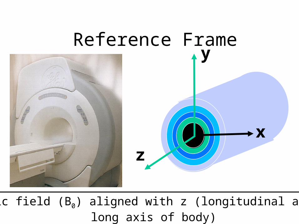
Reference Frame

Magnetic field (B0) aligned with z (longitudinal axis and long axis of body)

y

x

z

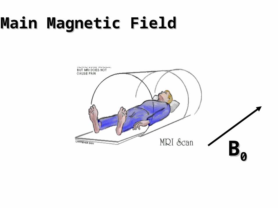
Main Magnetic FieldMain Magnetic Field

BB00

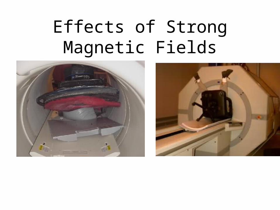
Effects of Strong Magnetic Fields

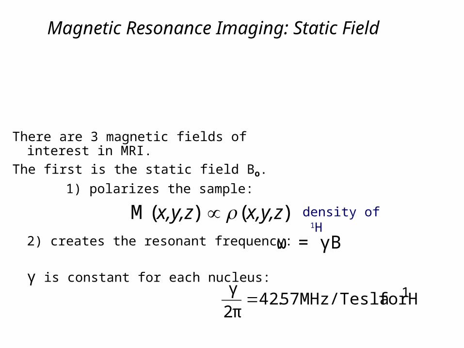
Magnetic Resonance Imaging: Static Field

There are 3 magnetic fields of interest in MRI.

The first is the static field Bo.

1) polarizes the sample:

2) creates the resonant frequency:

γ is constant for each nucleus:

)( )(M x,y,zx,y,z density of 1H

Hfor MHz/Tesla 57.42π2

γ 1

ω = γB

x

y

z

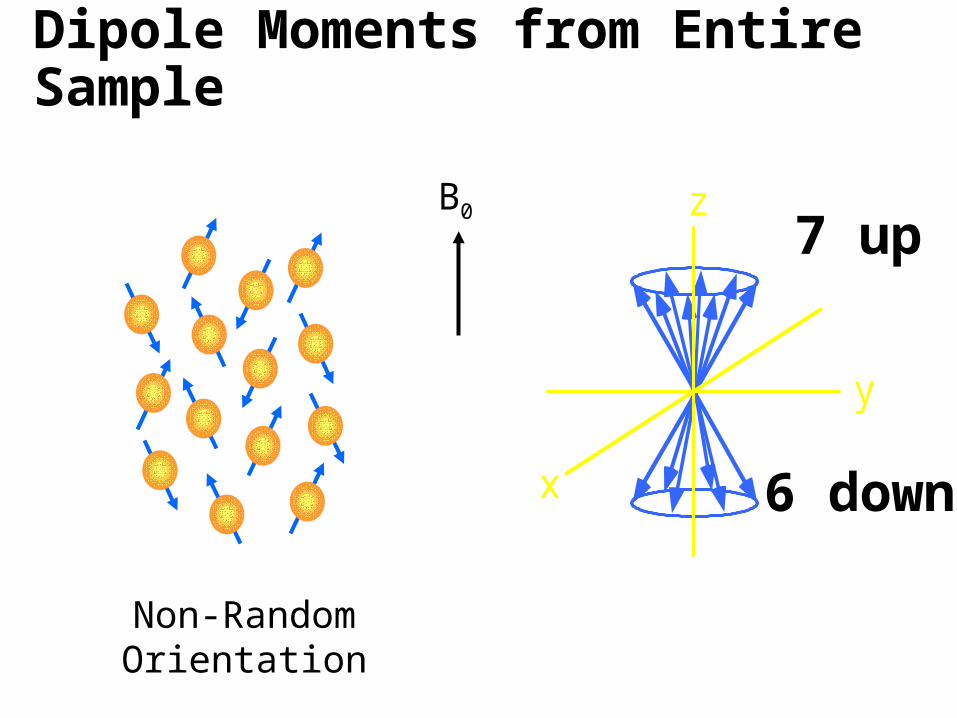
Dipole Moments from Entire Sample

B0

Non-RandomOrientation

7 up

6 down

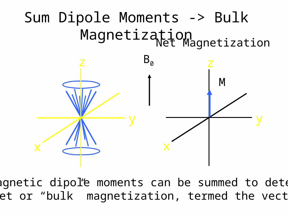
Net Magnetization

Sum Dipole Moments -> Bulk Magnetization

The magnetic dipole moments can be summed to determinethe net or “bulk” magnetization, termed the vector M.

B0

M

x

y

z

x

y

z

Static Magnetic Field (B0)

Bore(55 – 60 cm)

Shim(B0 uniformity)

Magnetic field (B0)

Body RF(transmit/receive)

GradientsGradients

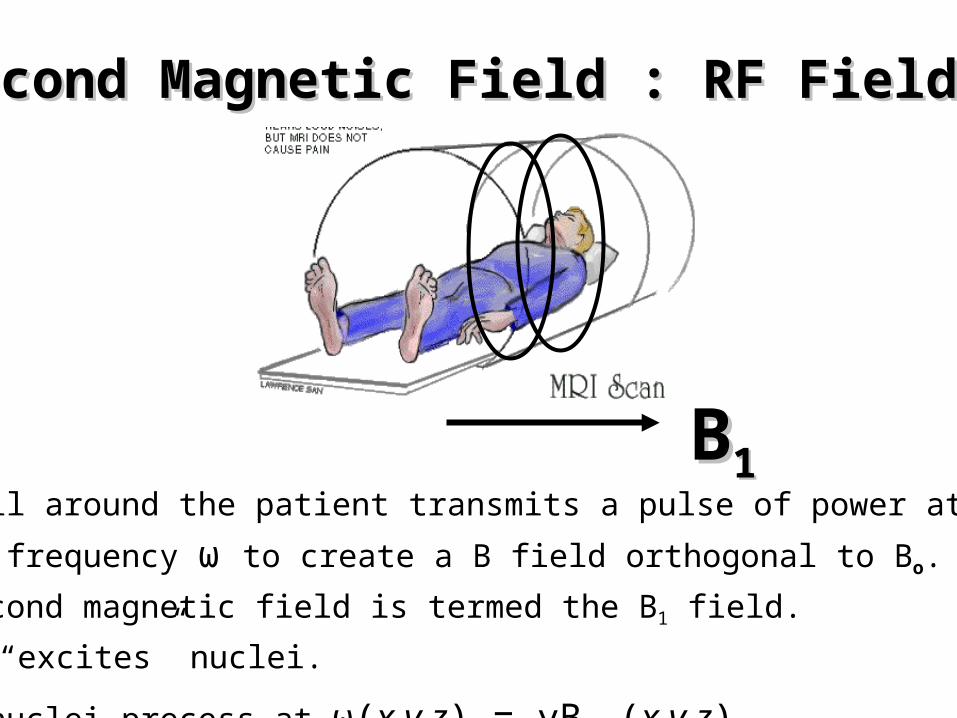
Second Magnetic Field : RF FieldSecond Magnetic Field : RF Field

BB11An RF coil around the patient transmits a pulse of power at the

resonant frequency ω to create a B field orthogonal to Bo.

This second magnetic field is termed the B1 field.

B1 field “excites” nuclei.

Excited nuclei precess at ω(x,y,z) = γBo (x,y,z)

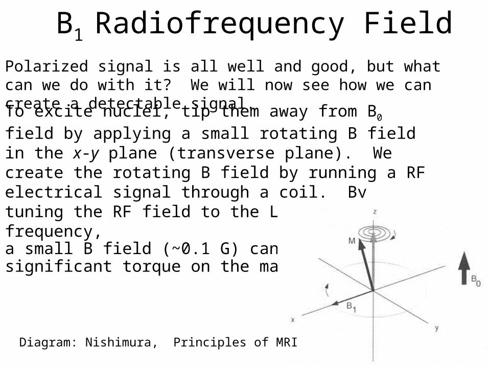
Polarized signal is all well and good, but what can we do with it? We will now see how we can create a detectable signal.

To excite nuclei, tip them away from B0 field by applying a small rotating B field in the x-y plane (transverse plane). We create the rotating B field by running a RF electrical signal through a coil. By tuning the RF field to the Larmor frequency,a small B field (~0.1 G) can create a significant torque on the magnetization.

B1 Radiofrequency Field

Diagram: Nishimura, Principles of MRI

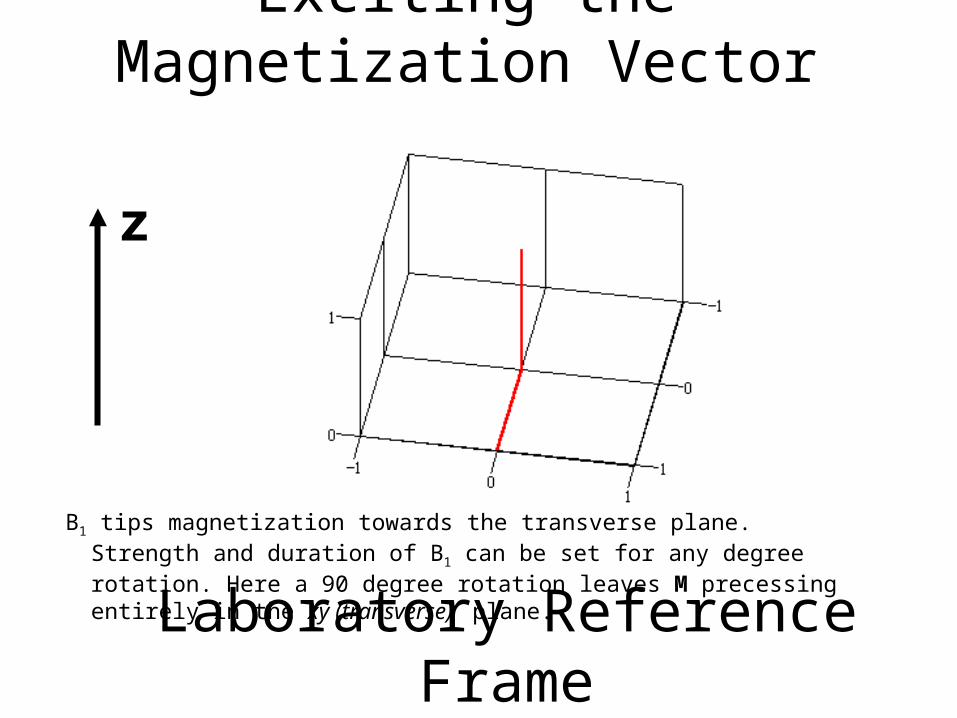
Exciting the Magnetization Vector

z

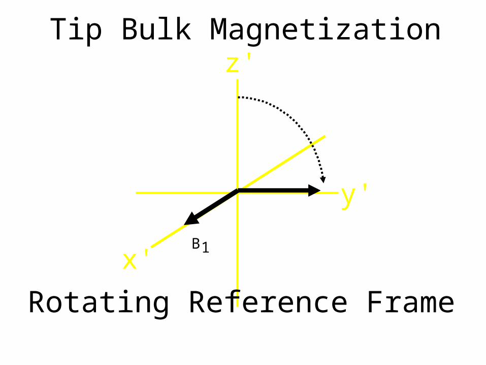
B1 tips magnetization towards the transverse plane. Strength and duration of B1 can be set for any degree rotation. Here a 90 degree rotation leaves M precessing entirely in the xy (transverse) plane.

Laboratory Reference Frame

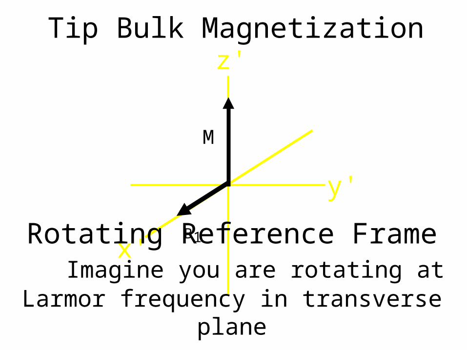
Tip Bulk Magnetization

x'

y'

z'

M

B1

Rotating Reference FrameImagine you are rotating at Larmor frequency in transverse plane

Tip Bulk Magnetization

x'

y'

z'

B1

Rotating Reference Frame

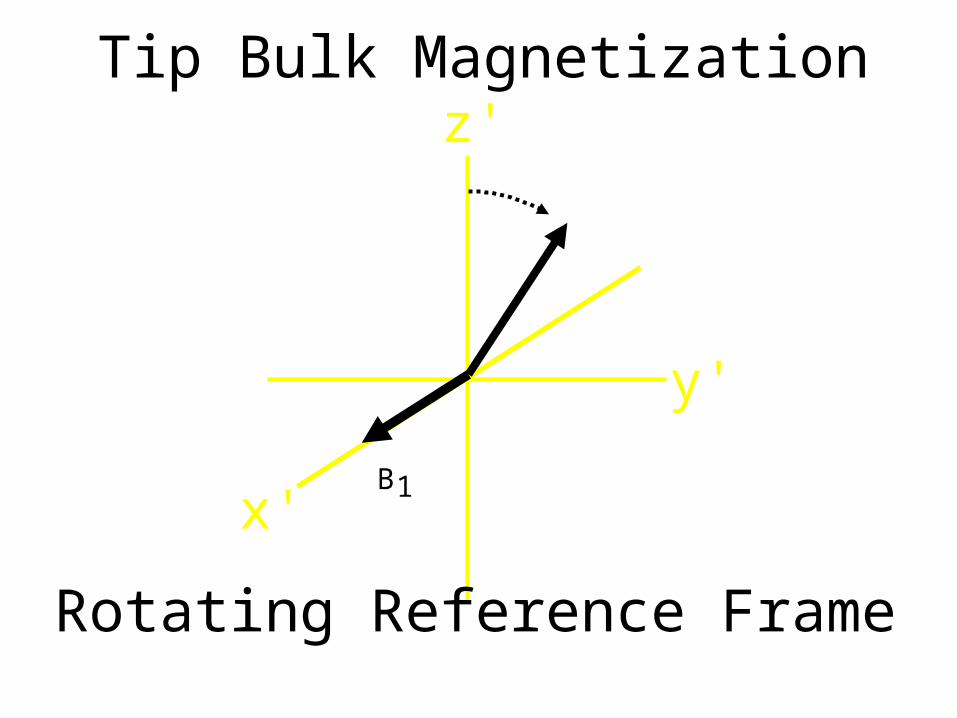
Tip Bulk Magnetization

x'

y'

z'

B1

Rotating Reference Frame

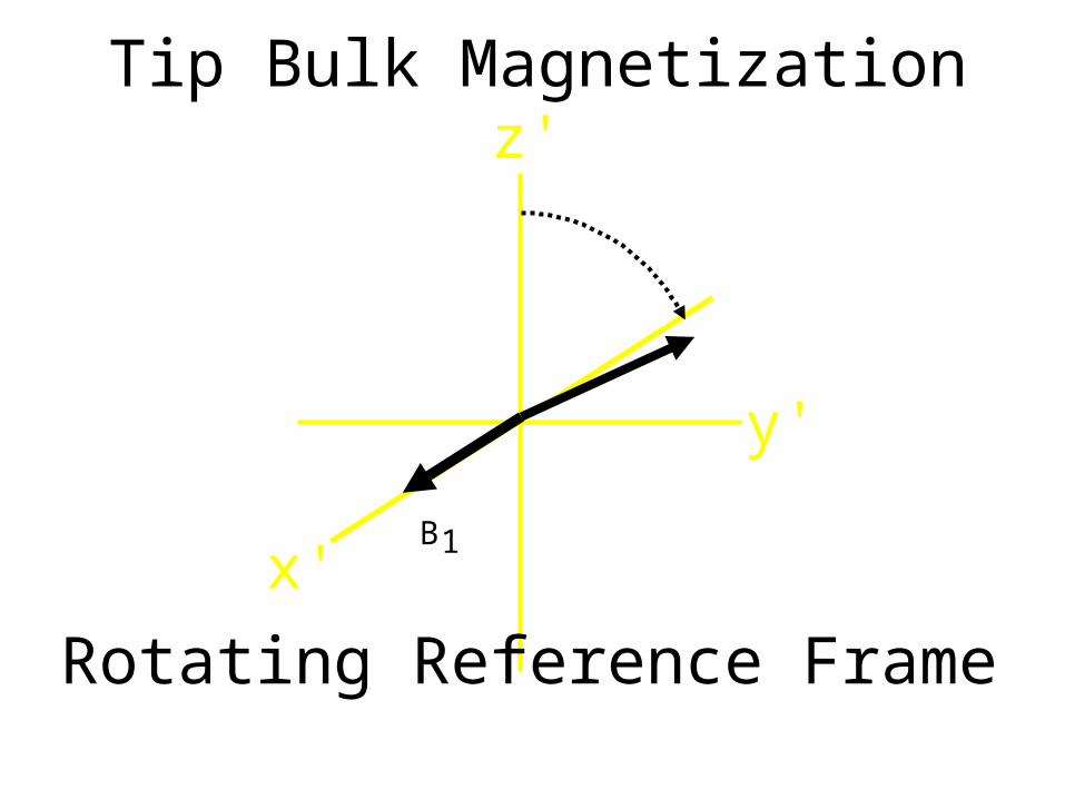
Tip Bulk Magnetization

x'

y'

z'

B1

Rotating Reference Frame

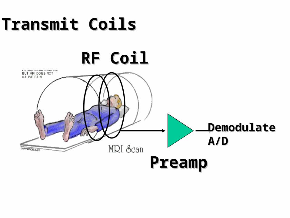
Transmit Coils Transmit Coils

PreampPreamp

Demodulate Demodulate A/DA/D

RF CoilRF Coil

Static Magnetic Field (B0)

Bore(55 – 60 cm)

Shim(B0 uniformity)

Magnetic field (B0)

Body RF(transmit/receive)

GradientsGradients

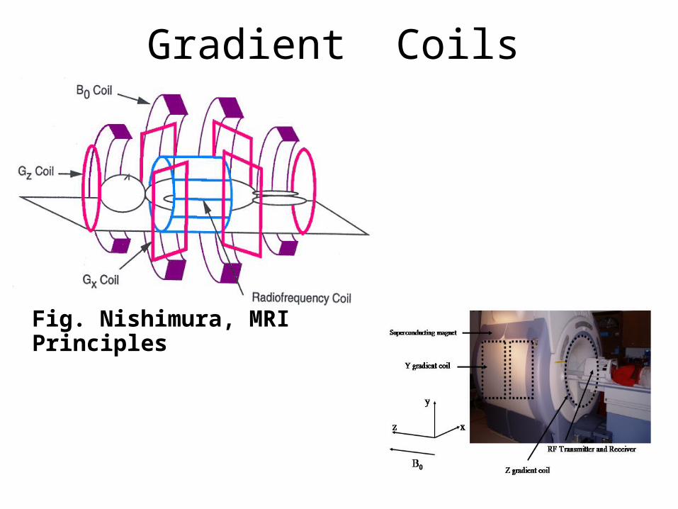
Gradient Coils

Fig. Nishimura, MRI Principles

Spin Encoding

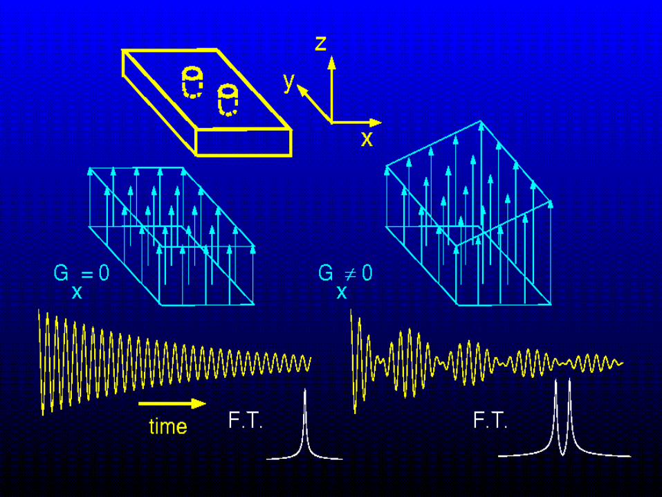
Magnetic ResonanceThe spatial location is encoded by using gradient field coils around

the patient. (3rd magnetic field) Running current through these coils changes the magnitude of the magnetic field in space and thus the resonant frequency of protons throughout the body. Spatial positions is thus encoded as a frequency.

The excited photons return to equilibrium ( relax) at different rates. By altering the timing of our measurements, we can create contrast. Multiparametric excitation – T1, T2

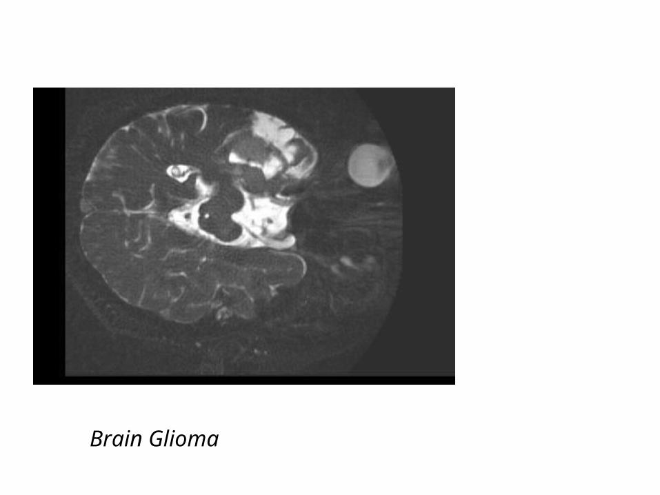
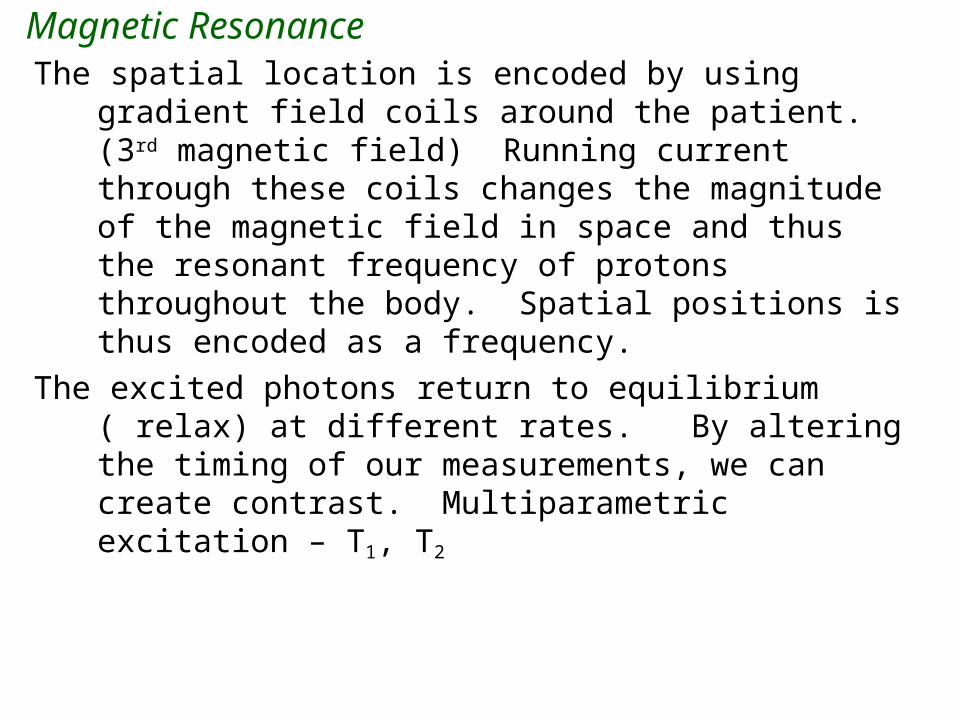
Brain Glioma

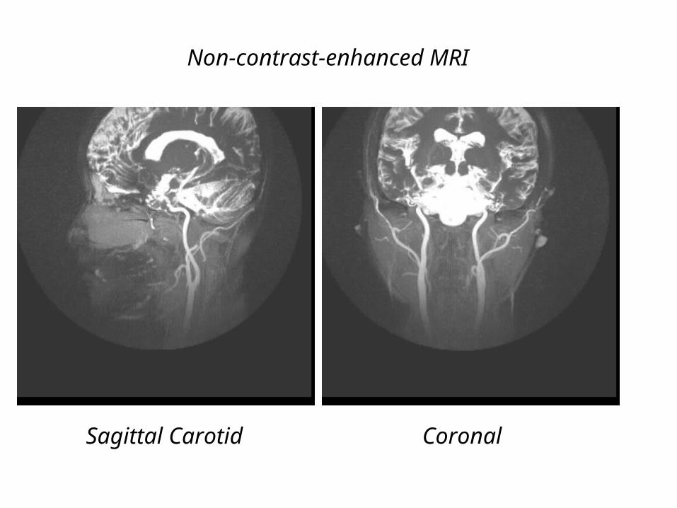
Sagittal Carotid

Non-contrast-enhanced MRI

Coronal

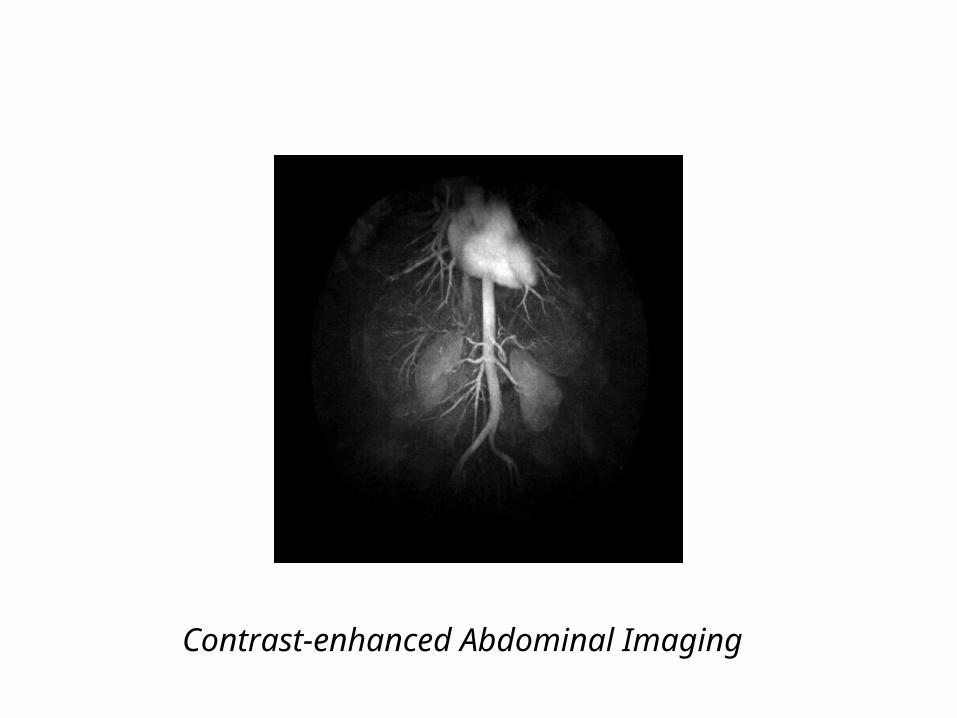
Contrast-enhanced Abdominal Imaging

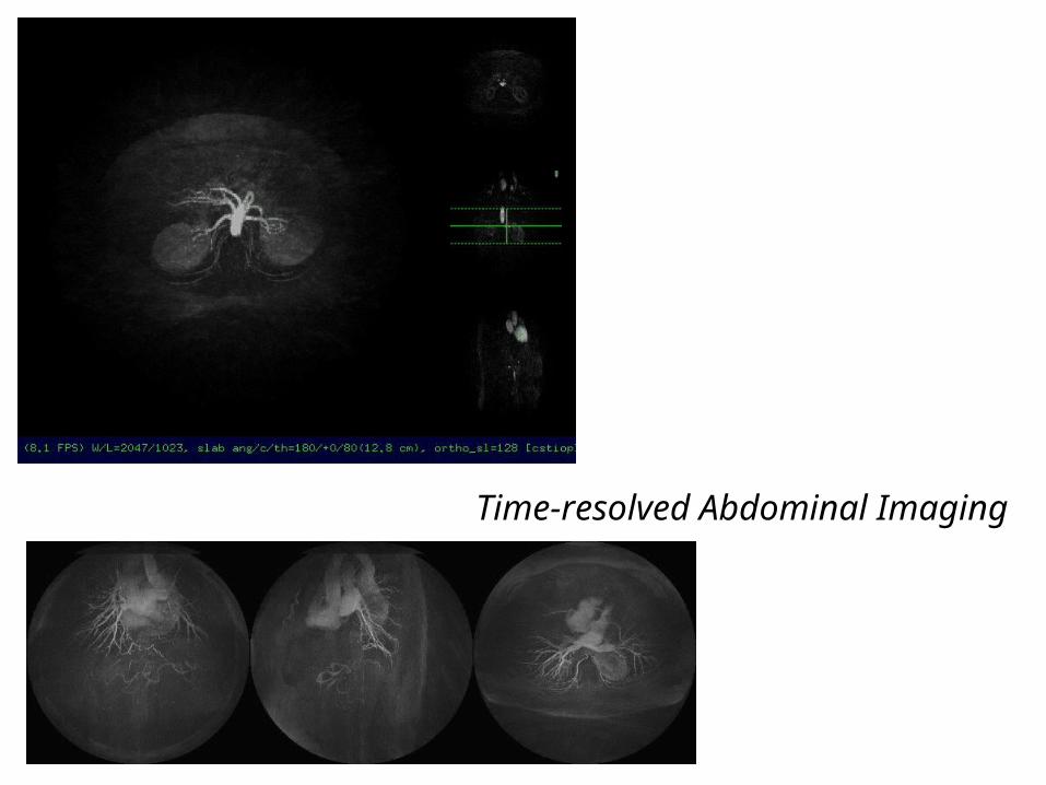
Time-resolved Abdominal Imaging

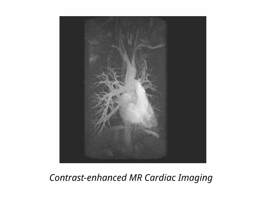
Contrast-enhanced MR Cardiac Imaging

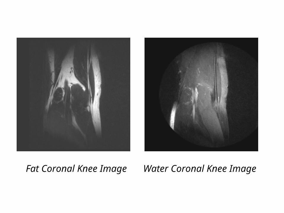
Fat Coronal Knee Image Water Coronal Knee Image

Comparison of modalities

Why do we need multiple modalities?

Each modality measures the interaction between energy and

biological tissue.

- Provides a measurement of physical properties of tissue.

- Tissues similar in two physical properties may differ in a third.

Note:

- Each modality must relate the physical property it measures to normal or abnormal tissue function if possible.

- However, anatomical information and knowledge of a large patient base may be enough.

- i.e. A shadow on lung or chest X-rays is likely not good.

Other considerations for multiple modalities include:

- cost - safety - portability/availability

Comparison of modalities:X-Ray

Measures attenuation coefficient

Safety: Uses ionizing radiation

- risk is small, however, concern still present.

- 2-3 individual lesions per 106

- population risk > individual risk

i.e. If exam indicated, it is in your interest to get exam

Use: Principal imaging modality

Used throughout body

Distortion: X-Ray transmission is not distorted.

),,(μ zyx

Comparison of modalities:Ultrasound

Measures acoustic reflectivity

Safety: Appears completely safe

Use: Used where there is a complete soft tissue and/or fluid path

Severe distortions at air or bone interface

Distortion:

Reflection: Variations in c (speed) affect depth estimate

Diffraction: λ ≈ desired resolution (~.5 mm)

),,R( zyx

Comparison of modalities:Magnetic Resonance (MR)Multiparametric

M(x,y,z) proportional to ρ(x,y,z) and T1, T2.(the relaxation time constants)

Velocity sensitive Safety: Appears safe

Static field - No problems

- Some induced phosphenes

Higher levels - Nerve stimulationRF heating: body temperature rise < 1˚C - guideline

Use: Distortion: Some RF penetration effects

- intensity distortion

T/s 10dt

dB

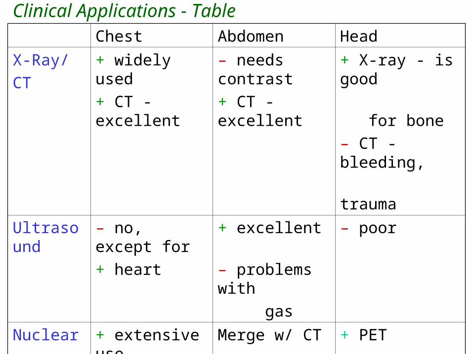
Clinical Applications - TableChest Abdomen Head

X-Ray/

CT

+ widely used

+ CT - excellent

– needs contrast

+ CT - excellent

+ X-ray - is good

for bone

– CT - bleeding,

trauma

Ultrasound – no, except for

+ heart

+ excellent

– problems with

gas

– poor

Nuclear + extensive use

in heart

Merge w/ CT + PET

MR + growing

cardiac

applications

+ minor role + standard

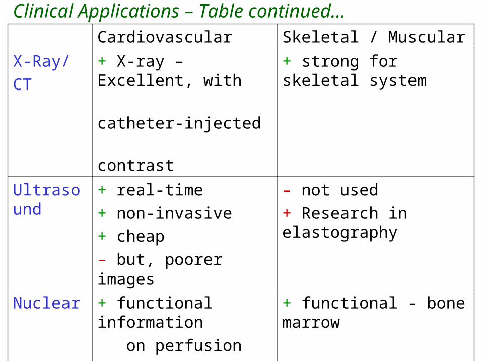
Clinical Applications – Table continued…Cardiovascular Skeletal / Muscular

X-Ray/

CT

+ X-ray – Excellent, with

catheter-injected

contrast

+ strong for skeletal system

Ultrasound + real-time

+ non-invasive

+ cheap

– but, poorer images

– not used

+ Research in elastography

Nuclear + functional information

on perfusion

+ functional - bone marrow

MR + getting better

High resolution

Myocardium viability

+ excellent

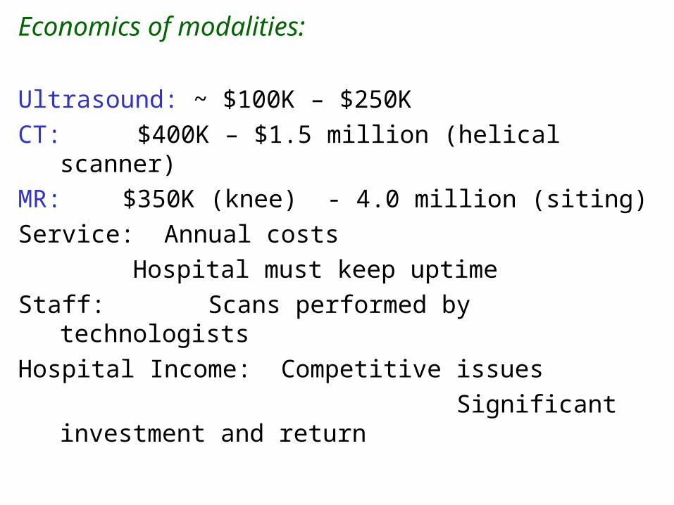
Economics of modalities:

Ultrasound: ~ $100K – $250K

CT: $400K – $1.5 million (helical scanner)

MR: $350K (knee) - 4.0 million (siting)

Service: Annual costs

Hospital must keep uptime

Staff: Scans performed by technologists

Hospital Income: Competitive issues

Significant investment and return