Introduction - Aalborg Universitetprojekter.aau.dk/projekter/files/17606498/CAE... · Web viewAnother LS-DYNA material model, *MAT _083, is sometimes also used in these types of analyses

DMS10Spring 2009

CAE Correlation of Automotive foam material using LS-DYNA 971

Mentor:Jesper Christensen Lars Rosgaard Jensen

PrefaceThis report is the outcome of a final year M.Sc. project conducted at Jaguar Land Rover

Whitley engineering centre in Coventry, United Kingdom in the spring of 2009.

This report consists of a main part, appendices and 4 DVDs. In addition to the main report and

the appendices, all FEM models, results and additional data referred to throughout the report

can be found on these DVDs.

The referencing method used in this report is modelled after the Harvard method, where the

reference setup is [Author, publication year]

In connection with this report the author would like to express his appreciation to Mr.

Jonothan Bowen of Jaguar Land Rover and Mr. Eduardo Arvelo of Advanced Simtech for

their involvement and commitment to this project.

The author would also like to express his utmost appreciation to Mr. Christophe Bastien of

Coventry University, for his dedication and assistance, and without whom this project would

never have been.

Title: CAE Correlation of Automotive foam material using LS-DYNA 971Semester: DMS10Project period: 02 / 02 / 2009 – 03 / 06 / 2009ECTS: 30Mentor: Lars Rosgaard Jensen

_________________________________[Jesper Christensen]

Number of reports printed: 5 Number of pages: 75Number of appendices: 5 Enclosed: 4 DVDs

SYNOPSIS:This report commences with a description of the purpose of conducting this project. Next an explanation of how the physical testing of the foam samples were conducted follows. The next focus of attention is a mathematical explanation of the b spline algorithm that has been programmed into a post process macro in order to extract the data needed to conduct the subsequent FEM correlation. This post process macro is enclosed.Subsequently the physical testing method is summed up and weaknesses in this procedure are pointed out. The culmination of this is a list of recommendations intended to be used for future testing.Thereafter the focus is aimed upon explaining the FEM correlation process, including a complete description of the general FEM model which utilises the *MAT_057 material model. The outcome of this correlation process is 600 correlated models, which are all enclosed in *.key format. The correlation results, including detailed information of the model variables are enclosed in a html file. The final focus of attention explores the limitations of the used *MAT_057 material model and compares this to the alternative *MAT_083 material model.The outcome is that that the *MAT_083 model is the better of the two when accounting for rate effects, but the *MAT_083 material model show signs of inconsistency when combined with a specific element formulation and a specific solver.

Table of contents

Summary....................................................................................a

1. Introduction..........................................................................12. H-Point and SGRP-point......................................................3

2.1 Occupant positioning........................................................................................................32.2 Occupant safety.................................................................................................................6

3. MIRA test setup....................................................................74. Post processing of MIRA test data...................................10

4.1 Curve fitting algorithm...................................................................................................124.2 B spline algorithm...........................................................................................................154.3 V6 post process macro....................................................................................................184.4 Comparison of V3 and V6 macros..................................................................................234.5 Accuracy of V6 post process macro...............................................................................264.6 Criteria for post processing MIRA test data...................................................................28

5. Evaluation of physical testing...........................................365.1 MIRA test results............................................................................................................365.2 Strain values....................................................................................................................405.3 Load cell..........................................................................................................................415.4 Test specimens................................................................................................................425.5 Plus Pad results...............................................................................................................435.6 Recommendations for future testing...............................................................................45

6. LS-DYNA 971 keyword FEM correlation...........................466.1 General FEM model description.....................................................................................466.2 Determination of damping constant................................................................................516.3 Correlation results...........................................................................................................52

7. *MAT_057 - *MAT_083........................................................557.1 Theoretical comparison...................................................................................................557.2 *MAT_057 and *MAT_083 results comparison............................................................587.3 Practical comparison.......................................................................................................617.4 Strain rate effects............................................................................................................687.5 Shape effects...................................................................................................................737.6 Recommendations for choosing a material model..........................................................74

8. Conclusion..........................................................................75References.................................................................................iAppendix A............................................................................... iiAppendix B.............................................................................. iiiAppendix C.............................................................................. iv

Appendix D..............................................................................viAppendix E................................................................................x

SummaryThis report is the documentation of a DMS10 project conducted at Jaguar Land Rover in

Whitley, Coventry, United Kingdom, in the spring semester of 2009.

The overall aim of the project documented by this report and associated appendices is to

determine material characteristics as a function of strain rates, for foam material used for

seats in various vehicle programs manufactured by Jaguar Land Rover (JLR). The final

outcome is to be fully developed FEM material models to represent the material

characteristics for a given location of a particular foam. These material models are all

compliant with LS-DYNA keyword 971.

These FEM material models are based upon physical test data.

Initially the report explains why this project is of great interest to JLR, and thereby the

reasons for conducting it.

The next focus of attention is concerned with the physical testing procedure. This includes a

detailed description of the methodology and also points out strengths and weaknesses in the

procedure. The culmination of these discussions is a list of recommendations intended to be

used as a guide for future testing of a similar nature.

Thereafter the focus is aimed upon the post processing part of the obtained test data, in order

to be able to utilise this in relation to the overall aim. This has been conducted by

programming various Excel, Visual Basic, macros for post processing. This includes a B

spline algorithm that can be used to curve fit the test data in order to decrease unwanted

“noise” as experienced in some of the physical test data. This B spline algorithm is complete

with mathematical documentation.

The following topic is the actual FEM correlation process, this has been conducted using the

LS-DYNA keyword 971 *MAT_057 material model. The FEM correlation process contains a

total of 600 correlated FEM models, i.e. a total of 600 correlated *MAT_057 material models.

The final topic focuses upon comparing the alternative *MAT_083 material model to the

*MAT_057 material model. In addition some of the limitations of the *MAT_057 material

model is explored. These include rate effects, shape effects and ability to control energy

dissipation during a load / unload cycle.

1. IntroductionThe aim of this report is to solve a problem set forth by Jaguar cars limited. The problem is

concerned with the material characteristics of the foam used to produce the seats used for four

model ranges manufactured by Jaguar / Land Rover (JLR). The four ranges in question are:

Jaguar:

o XK (X150)

o XF( X250)

o XJ (X358)

Land Rover:

o Range Rover (L322)

The terms in parenthesis represent the model IDs used internally at JLR, and will be referred

to throughout this report.

The foam for the seats used in these four model ranges are all supplied from the same external

subcontractor: Lear foam. The foam is thought to be made from a type of Urethane foam,

although this has not been confirmed by Lear foam. The manufacturing process can briefly be

described as follows:

The seat foaming is produced by pouring liquid chemicals into a mould, which are

subsequently allowed to harden. The subcontractor has vividly described this process as a

“black art”. This is to be interpreted in terms of material characteristics, because no specific or

detailed material characteristics are supplied from the subcontractor.

Important parts of automotive seat design include occupant positioning and occupant safety.

These are the two major reasons for Jaguar Land Rover to be interested in conducting this

project. These reasons will be further outlined in chapter 2.

The FEA analyses conducted at JLR in context to occupant positioning and occupant safety

are conducted in LS-DYNA 971 keyword format. Therefore all FEA analysis and associated

discussions documented throughout this report will be related to the LS-DYNA 971 keyword

format.

The outcome of this report aims to enable JLR to:

1. Dictate the desired material characteristics of the seating foam for the individual

model range to the subcontractor.

2. Set up a complete material model in the LS-DYNA 971 keyword format to model the

seating foam in question.

Jesper Christensen 1. Introduction 1 / 75

3. Verify the above material model used to model the seating foam in various FEM

analyses.

Because of the described manufacturing process, a single seating foam is expected to have

different characteristics in different areas of the seat.

Based on the above statements, the governing task of this report can be described as:

“Find and verify engineering stress vs. engineering strain curves representing the

characteristics of the seat foam in the particular area of a seat from a particular model

range”.

The initial steps for the governing task stated above have already been made. The physical

testing has been conducted, the post process part has been initiated, and the LS-DYNA part of

the project has also been initiated. The problem is that none of these steps, with the exception

of the physical testing have been documented. Therefore, the task documented by this report

is to use this previous work as a type of steppingstone, outlining the path in between, and

highlighting the strengths, weaknesses, assumptions made, the implication of these and

recommendations for future testing and correlation assignments. Never the less, the overall

governing task remains identical to the one stated above.

In addition to the overall governing task, a stretch objective has been set forth. The purpose of

which is to further analyse the strength and the weakness of the material model set up in step

2 and step 3 above. In addition, the possibilities of using alternative material models to the

one previously defined will be examined. In this context it should be noted that all material

models must be LS-DYNA keyword 971 compatible. Therefore, the two stretch objectives

can be formulated as stated below:

4. Examine the limitations of the material model set forth in step 2 and step 3 above.

5. Search for alternative material models in LS-DYNA keyword 971 format that can be

used to model the foam in question.

The five steps listed above will all be elaborated throughout the individual chapters and

associated appendices of this report. Before the actual correlation process commences it is of

great importance to further substantiate the major reasons for Jaguar Land Rovers interest in

the foam correlation process and data that is to be the outcome of this report. This will be the

focus of attention in the next chapter.

Jesper Christensen 1. Introduction 2 / 75

2. H-Point and SGRP-pointThe purpose of this chapter is to outlay some of the major reasons for Jaguar Land Rover to

be interested in the foam correlation process that is the basis of this report.

The contents of this chapter are primarily based upon information provided by JLR and

information supplied by SAE international.

In chapter 1 it was stated that important parts of automotive seat design included occupant

positioning and occupant safety.

2.1 Occupant positioning

One of the major aims of this report is to enable JLR to dictate the desired material

characteristics of the seating foam for the individual model range to the subcontractor.

The reasons for JLR to set forth this specific aim for this project can all be linked to two

terms; the H-point and the SGRP-point.

The H-point is also known as the hip point, and is a well known term within the automotive

industry. The H-point relates to a physical point on a crash test dummy, which is intended to

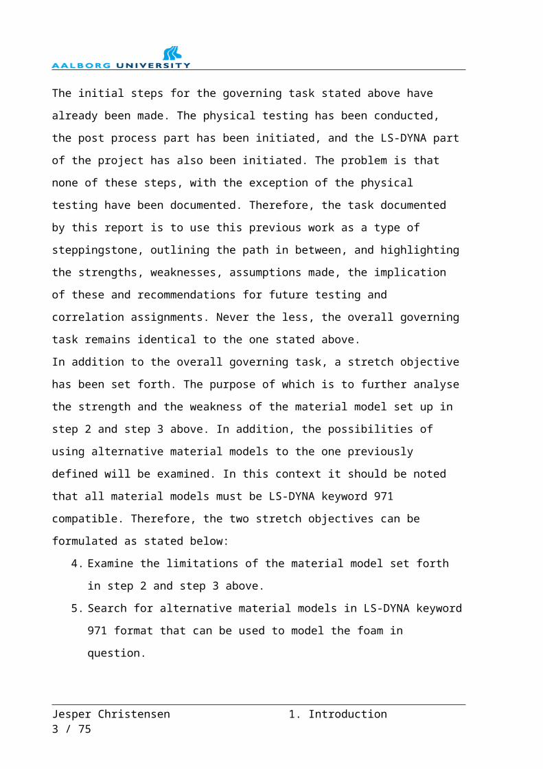
represent the theoretical point on a human body around which the torso rotates. Figure 1

below, is an illustration of the H-point location.

Figure 1, illustration of H-point location on a crash test dummy.

In the illustration above, the y-coordinate of the H-point is positioned in the symmetry line of

the crash test dummy in the yz-plane.

The Seating Global Reference Point, SGRP point, is to be defined for each individual vehicle

programme. It is essentially from this datum point that all the design related to the drivers

position is carried out. I.e. the location of the steering wheel, switches, pedals, etc. are all

defined from this single point.

Prior to selling a road car in any market it must comply with the given legislation. In order to

provide evidence that the legislation has not been violated, numerous tests must be carried out

on the road car in question. In the case of JLR and any other manufacturer which mass

produces vehicles it is beneficial to obtain a vehicle type approval. Obtaining this approval

Jesper Christensen 2. H-Point and SGRP-Point 3 / 75

allows for not testing each individual road car for the complete series of tests dictated by the

legislation, although certain basic tests still need to be conducted on the individual vehicle. In

the UK a vehicle type approval can be granted by the Vehicle Certification Agency, the VCA:

“VCA is the designated UK Approval Authority and Technical Service for type approval to all

automotive European Community (EC) Directives and the equivalent United Nations

Economic Community for Europe (ECE) Regulations. Vehicle Type Approval is the

confirmation that production samples of a design will meet specified performance standards.”

[VCA, 2009]

One of the tests that must be passed in order to obtain a vehicle type approval is related to the

H-point and the SGRP point, this test could e.g. be the ECE17.

The test procedure can briefly be described as placing a crash test dummy in the driver’s seat

and then checking that certain requirements are met.

The requirements all relate to the positioning and the drivers view of the road.

The crash test dummy must comply with SAE J826 standards. This includes the geometrical

dimensions of the dummy, which represents 50 percentile of the population. Figure 2 is an

illustration of the dummy positioned in the seat.

Figure 2, illustration of crash test dummy positioned in driver’s seat.

The 4 points denoted in Figure 2 indicates the locations were some of the checks in the test

are conducted. Point 1 is the point from where the required minimum viewing angles are

measured. Point 2 is the location of the dummy’s hands, which must be able to reach the

steering wheel etc. Position 4 is the location of the dummy’s feet which must be able to reach

the foot pedals. Point 3 represents the H-point of the dummy. The distances from this point,

i.e. point 3, to point 1, 2 and 4 respectively are defined in the test procedure. These distances


are measured in three dimensions, but the y-coordinate of the H-point is, as illustrated in

Figure 1, located in the dummy’s line of symmetry in the yz-plane. The angle of the seat back

in relation to the z-axis is also dictated by the test procedure.

When the dummy is positioned in the seat, the test states that the coordinates of the H-point of

this specific dummy must be located within a square having a side length of maximum 25mm,

centred in the SGRP point in the xz-plane. This is illustrated in Figure 3, which can be

perceived as a close up of point 3 in Figure 2.

Figure 3, H-point and SGRP point.

The side length of 25 mm is a legal requirement, however at JLR this requirement has been

sharpened by specifying a side length of 10 mm. Considerations relating to passing this

specific test are most often introduced at an early stage in the design process.

In order to be able to fulfil the objective illustrated by Figure 3 it is therefore necessary to

calculate where the dummy’s H-point will be when it is placed in the driver’s seat. In order to

do this as accurately as possible, it is necessary to know the characteristics of the seating foam

used. This is one of the major reasons for conducting the foam correlation of this report.

The importance of being able to predict this location accurately at an early stage in the design

process is further underlined when observing the ideal project plan for developing a new

vehicle program, which JLR strides to obtain. A simplified version of this is illustrated in

Figure 4.

Figure 4, simplified ideal project plan for new vehicle program.


The UNV stage in Figure 4 is the under body vehicle stage, which covers tasks such as design

of deformation zones, suspension, location of seating mounts etc. The UPV stage, or the

upper body stage briefly entails tasks such as body panels, roof line etc.

The completion of these two stages is marked by the final data judgement event, after this

point only minor is allowed on the vehicle program. The next stage is concerned with setting

up the manufacturing line. Once this stage is complete, the 1st prototype is built. Only at this

point can the calculations relating to the H-point and SGRP point as described above be

verified by physical testing. If the calculations prove to be inaccurate, changes at this stage are

very expensive in terms of resource and money.

Job 1 is the time where the first production vehicle rolls of the production line.

Observing Figure 4 reveals another reason for the JLR interest in this correlation project,

because the more accurately the SGRP / H-point location can be calculated in the initial UNV

phase, the less likely it is that changes will be made between the 1st prototype and job 1.

2.2 Occupant safety

The first major reason for Jaguar Land Rover’s interest in this project as described above

suggests that only the foam characteristics from quasi-static or low strain rate tests are of

interest. However the other major reason implies that also foam characteristics at larger strain

rates are of interest, this is related to occupant safety.

The expression safety can be understood in many ways. However, in this particular case it is

to be understood in terms of a car crash and its influence on the passengers of the car(s) in

question, e.g. whiplash effects or Head Injury Criteria (HIC) which is used to determine

whether damages are fatal or not. In an attempt to improve the accuracy of a given crash

analysis it is of great importance to implement the characteristics of the seating foam when

setting up an FEA model.

This is the second major reason for Jaguar Land Rover’s interest in the work documented by

this report. In addition it underlines the fact that not only the quasi-static foam characteristics

are of interest but also the foam characteristics at higher strain rates are of great interest.

The next chapter will explain the testing procedure used to conduct the physical testing of the

seat foam in greater detail.


3. MIRA test setupThis chapter aims to describe the method and procedure used to conduct the physical testing

of the seat foams. This part of the project was conducted in 2008 and was therefore completed

before the author of this report became involved in the project.

The actual testing of the seat foams was not conducted by Jaguar Land Rover; these were

conducted by the testing provider: MIRA.

Therefore, this chapter will solely be based upon data and information supplied by JLR and

MIRA.

The purpose of the test was to obtain curves plotting force in N vs. compression in mm. for

both loading and unloading scenarios. These curves are intended to form the basis of the LS-

DYNA material models for the FEM crash analysis.

Selection of seats, the test speeds, the specimen geometry etc. were all dictated by JLR. The

test was set up to compress the foam specimens by 80% of their original height, i.e. a strain

value of 0.8.

Four different test speeds were defined: 10 mm/min, 100 mm/min, 250 mm/min and

500 mm/min.

The geometry of the test specimens was chosen to be cylindrical in an attempt to minimise the

influence of shape effects.

Experience showed that the seats had different characteristics in different part of the seat.

Therefore, the specimens were to be cut directly out of actual seats. A cutting tool was

designed to cut the specimens from the seats. Figure 5 illustrates the cutting tool.

Figure 5, cutting tool.

Figure 6 illustrates examples of test specimens; note the difference in height of the individual

test specimens.

Jesper Christensen 3. MIRA test setup 7 / 75

Figure 6, examples of test specimens.

As Figure 6 indicates, some of the specimens vary significantly in height. In general, three

specimen heights exist: 50mm, 25mm, and 15mm. The majority of the specimens are

approximately 50mm in height. All test specimens have a diameter of approximately 50mm.

As many specimens as possible were cut out of the individual seats. Figure 7 illustrates L322

seat foam with the specimens cut out.

Figure 7, L322 seat foams with specimens cut out.

As previously stated the seats are from four different JLR vehicle programs. Each vehicle

program contains seat variations due to various seat functions, e.g. climate controlled seats or

comfort seats. This leads to additional specimens, a total of 652 specimens being cut out of

the seats. A complete overview of the seat specimens and their original location on the

individual seats is enclosed on DVD 1 in the file: “Foam_samples_matrix.xls”

In addition to these specimens JLR utilises additional foam padding for the head rests and to

“harden up” the feel of the seat in e.g. sports seats. Specimens were also made from this

additional padding. The additional padding is denoted “Rowa” and “Plus Pad” respectively.

These added specimens mean that the combined number of specimens is 686. The 686

specimens, the 4 test speeds and the fact that loading as well as unloading were to be tested

brought the total number of tests to 5488.


However, the loading and unloading tests were conducted in immediate succession, i.e. two

tests were conducted per one test setup.

In an attempt to minimise the possible effects of viscoelasticity the specimens were allowed to

between tests, this was done by conducting e.g. all 10 mm / min tests before commencing the

100 mm / min tests.

The test setup basically consisted of a compression test machine and a 1000 N load cell. The

test setup can be seen in Figure 8.

Figure 8, experimental test setup.

The overall test procedure can briefly be described as follows:

1. Cut the foam specimens from the chosen locations and label them accordingly.

2. Measure the diameter, height and weight of each individual specimen.

3. Conduct the loading and unloading tests for all specimens at a test speed of 10

mm/min, a strain value of 0.8 must be reached.

4. Repeat step 3 for test speeds of 100 mm/min, 250 mm/min and 500 mm/min.

The price for these tests, including a test report and a total of 800 specimens was quoted at

£14360 + VAT. The reason for 800 specimens is that additional square foam blocks were

tested, however these are of no interest in relation to this report.

The MIRA test data report is enclosed on DVD 1 in the file: “MIRA_test_data_report.pdf”.

The next chapter will focus on the post processing phase of the project, which includes

processing the obtained physical testing data in order to extract correlation curves and data to

be used as input for the FEM correlation models.



4. Post processing of MIRA test dataThe purpose of this chapter is to explain the method that has been used to post process the test

data from MIRA as well as preparing input data for use in the FEM correlation models. The

MIRA test results were given in the format of Excel files, i.e. *.xls. A more detailed

description of the contents of these files can be found in Appendix A.

At this point it would seem obvious to simply export the test result data and utilise these

directly in the LS-DYNA material model. However, closer inspection of the test data results

reveals that some of these contain unwanted “noise”, the amount of which varies greatly with

the individual specimen. Possible reasons for this noise will be addressed later in this report.

For the time being all that is established is that the noise exists. One of the more obvious

examples of the presence of noise can be seen in Figure 9, which illustrates the loading curve

of a specimen taken from a seat intended for the L322 vehicle program, i.e. a Range Rover.

Figure 9, loading curve for: L322-1-2- 500 mm/min, specimen 4.

Figure 9 clearly indicates the presence of noise because the force required to compress the

foam specimen is roughly zero, until the compression reaches a value of approximately 2 mm.

As previously stated, possible reasons for the noise will not be discussed at this point in the

report.

Now that the presence of noise in the test data results has been established, it is clear that the

test data can not be directly utilised as input for the LS-DYNA FEM models, before some

form of adjustment of the test data has been carried out.

Jesper Christensen 4. Post processing of MIRA test data 10 / 75

Due to this fact, the substantial amount of data and the systematic build up of the individual

*.xls files it was previously chosen to program an Excel macro in order to make these

adjustments and post process the test data results. As stated in chapter 1 the post processing

stage of the test data had already commenced before the author of this report became involved

in this project. Therefore, a post process macro had already been programmed. This macro is

denoted: “post-process_macro_V3.xls”, and is enclosed on DVD 1 and will henceforth be

referred to as: “V3”. However, no documentation for the V3 Excel macro existed. Therefore,

the author of this report set about analysing the programmed macro, in order to be able to

provide documentation for the macro. A general description of the V3 macro can be found in

Appendix B.

Following the completion of the V3 Excel macro analysis, it was clear that the adjustments of

the test data were done by the implementation of a curve fitting algorithm. A meeting between

the author of this report, and the programmer of the V3 macro was held, in order to confirm

the results of the analysis and to discuss the mathematical expressions utilised in the curve

fitting algorithm of the macro. During this meeting it became clear, that the programmer had

imported the curve fitting part of the code from elsewhere, and thus the mathematical

definitions of the curve fitting algorithm were not known. However, the accuracy of the V3

macro outputs had previously been supported, through the comparison of the results of an LS-

DYNA FEM model to those of the physical MIRA tests.

In the program code, the curve fitting function was denoted as being a Cubic spline, which is

not unlikely, as the polynomial expression has a cubic form, i.e. 3rd degree polynomial.

The reason why the mathematics behind the curve fitting algorithm used in the V3 macro has

not been further analysed is the desire to further improve the curve fitting technique. In

agreement with JLR it was decided to explore the options of adopting a more versatile and

flexible curve fitting algorithm complete with mathematical documentation. Part of the reason

for this was to improve the curve fitting algorithm for the test results in question, thereby

enabling a greater accuracy in reproducing the physical test data, without unwanted “noise”.

Another reason for exploring the options available was to provide Jaguar Land Rover with a

curve fitting algorithm that, with relative ease, could be utilised to post process data from

other physical testing or experiments.


4.1 Curve fitting algorithm

The following two sections are primarily based upon [Rasmussen, 1999] and [Rogers, 2001].

To meet the requirements of providing a more flexible and versatile curve fitting technique,

and based upon the exploration of the techniques available, the following four was chosen as

potential solutions:

Cubic spline

Bezier curve

B spline

Non Uniform Rational B spline (NURBS)

All of the curve fitting techniques listed above make use of so-called “control points”,

however the way they are implemented differ from algorithm to algorithm.

The general idea of control points is to “guide” or “control” the entire curve by use of these

control points.

The purpose of the following discussion is to compare the four proposed curve fitting

algorithms in order to select one of these to be implemented in the post process macro.

Cubic Spline

Although the curve fitting techniques to be replaced seemingly is a Cubic spline it was worth

investigating the characteristics of this curve fitting technique. Some of the advantages and

disadvantages of the Cubic spline are listed below:

Interpolates through a set of control points

The Cubic spline fits exactly through the control points

÷ Certain locations of the control points can lead to undesirable changes in the curve far

away from the control point in question.

As the new curve fitting algorithm is supposed to be versatile and flexible, the ability to

control the curve locally is rated very high. The lack of local control in the V3 macro,

believed to contain a Cubic spline algorithm, is illustrated in Figure 10, which represents the

unloading curve of a specimen taken from a seat intended for the Jaguar XK.


Figure 10, V3 post processed unloading curve for: X150-2-2-10 mm/min, specimen 8.

The yellow points represent the control points which as mentioned are a general feature of all

the curve fitting algorithms presented in this report. Note that the curve fit, i.e. the purple line

in Figure 10 passes directly through all of the control points, complying with the

characteristics of a Cubic spline.

Based upon the lack of local control the Cubic spline curve fitting algorithm is abandoned.

Bezier curve

The next curve fitting algorithm to be examined is the Bezier curve; some of the

characteristics of a Bezier curve are listed below:

Creates a curve through a set of control points

Partial local control

÷ Does not fit the curve exactly through all of the control points

÷ The shape of the curve is dominated by the end control points

÷ Moving one control point influences the entire curve.

Thus, the Bezier curve offers only partial local control, and is therefore abandoned in the

search of increased local control.

B spline

The next curve fitting algorithm is the B spline, which is a general case of the Bezier curve.

Two general B spline algorithms exist: The rational and the non rational, one of the

differences between the two is that the rational B spline can be used to reproduce curves

[Cambridge, 2009] and is therefore the only one of interest in this connection. Therefore the


phrase: “B spline” will refer to a rational B spline throughout the remainder of this report,

unless otherwise stated.

The main characteristics of the B spline are:


Variable local control

Variable smoothness of the curve


Thus the B spline offers the desired amount of local control, and is therefore a reel candidate

to replace the current curve fitting algorithm of the V3 macro.

NURBS

The final curve fitting algorithm to be analysed is the Non Uniform Rational B spline,

NURBS, which is a generalisation of the rational B spline, and does therefore have similar

characteristics to those of the B spline above:


Variable local control

Variable smoothness of the curve

Can exactly represent ordinary geometric shapes, such as lines, circles, ellipses,

hyperboles etc.


NURBS is a more recent curve fitting algorithm than e.g. a B spline, and is often used in CAD

software, due to its ability to perfectly represent ordinary geometric 2D and 3D shapes. The

price for this added accuracy is higher degree of complexity of the mathematical expressions.

The purple line of Figure 11 can be used to represent either a B spline or a NURBS. The blue

line in Figure 11 represents the curve to be fitted by the algorithm, and the yellow dots

represent the control points.


Figure 11, illustration of B spline and NURBS.

The purple line of Figure 11 is obviously not a good curve fit to the blue line, this is because

the purpose of the figure is to show the flexibility and local control associated with a B spline

or a NURBS. Figure 11 does not relate to any physical test data, but is to be regarded as a

visual illustration of the two curve fitting algorithms in question.

Therefore, the choice of a curve fitting algorithm is ultimately a choice between the NURBS

and the B spline. Given the fact, that the curve fitting ultimately is based upon subjective

visual assessments, it has been deemed that implementing the more complex NURBS

algorithm will not provide an equally large increase in the accuracy of the fitted curve.

Therefore, it has been chosen to utilise the B spline algorithm to replace the curve fitting

algorithm of the V3 macro.

4.2 B spline algorithm

As previously stated, the B spline in question is a rational B spline, because these can be used

to reproduce curves. The principle of a B spline is to interpolate a curve through specified

control points. The B spline curve will pass through the endpoints, i.e. P1 and P2, but not

necessarily through the internal control points, Pi. The control points, including the endpoints

can then be adjusted to fit the B spline curve to the desired geometry. The local control is

achieved by introducing so called blending functions, Ni,k which determines how much

influence the individual control point has. As previously stated, the smoothness of the curve


can also be adjusted. This is done by introducing the smoothness factor, k. If the variable is

denoted t, the polynomial for the B spline is given by equation :

The number of control points is equal to: n -1.

Before proceeding with the definitions it is of vital importance to further define the type of B

spline in question. This can be done by simply regarding the data plotted on Figure 9, which

immediately reveals that the curve is open on the right hand side, making the B spline open.

In addition it is desirable to being able to alter the 1st axis coordinates of the control points.

This effectively means that these values will no longer be equally spaced, as is the case of the

V3 macro. This means that the B spline will be non uniform. Thus the B spline to be

programmed can be defined as:

A rational, non uniform, open B spline.

Smoothness factor, k

The smoothness factor k effectively determines the continuity of the curve by ensuring the

number of derivatives that are continuous. Under normal circumstances, this value is set to 3

or 4. In effect, k can assume any integer value within the interval:

As the value of k increases, the curve will become increasingly smooth. The price for this

smoothness is that that curve will become increasingly controlled by the endpoints, and

thereby loose the local control. If then , i.e. the number of control points,

and the end points become all dominant, which means that the curve has become a Bezier

curve.

For this particular case the value of k has been set equal to 3, ensuring that the 1st derivative is

continuous, i.e. a 1st order continuity is achieved.

Knot vector,

The values of the entries in the knot vector are subsequently used to calculate the blending

functions, Ni,k(t). The values of the knot vector calculated here, are based upon a non uniform

knot vector with values proportional to the chord distances. The chord distance, Ci is the

direct distance between the individual control points, Pi, and is calculated by use of

Pythagoras’ theorem, as stated in equation :


In equation , Pxi represents the x- or 1st axis value, and Pyi represent the y- or 2nd axis value of

the point Pi.

The entries of the knot vector can then be calculated by the following expressions:

The number of entries in the knot vector will therefore be proportional to the smoothness

factor k, and the number of control points, n-1.

The knot vector will thus take the form:

The variable t will thus have to be found within the interval:

Blending functions, Ni,k(t)

As stated, the blending functions, also often denoted as basis functions, determine how much

influence the individual control point has on the curve in a given region. The blending

functions, Ni,k(t) are normalised functions, i.e. for any given k and t that complies with and ,

respectively the following statement is valid:

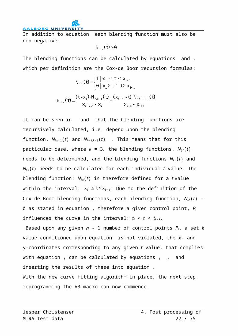
In addition to equation each blending function must also be non negative:

The blending functions can be calculated by equations and , which per definition are the Cox-

de Boor recursion formulas:

It can be seen in and that the blending functions are recursively calculated, i.e. depend upon

the blending function, Ni,k - 1(t) and Ni + 1,k - 1(t) . This means that for this particular case, where


k = 3, the blending functions, Ni,1(t) needs to be determined, and the blending functions Ni,2(t)

and Ni,3(t) needs to be calculated for each individual t value. The blending function: Ni,k(t) is

therefore defined for a t value within the interval: . Due to the definition of the

Cox-de Boor blending functions, each blending function, Ni,k(t) = 0 as stated in equation ,

therefore a given control point, Pi influences the curve in the interval: ti < t < ti + k.

Based upon any given n - 1 number of control points Pi, a set k value conditioned upon

equation is not violated, the x- and y-coordinates corresponding to any given t value, that

complies with equation , can be calculated by equations , , and inserting the results of these

into equation .

With the new curve fitting algorithm in place, the next step, reprogramming the V3 macro can

now commence.

4.3 V6 post process macro

As previously stated an Excel macro to post process the MIRA test data, named V3 already

exists. The main reason for reprogramming this is to adapt a better, more versatile and flexible

curve fitting technique, which has been selected to be a B spline.

Part of the V3 Excel macro has been reused in the V6 macro, although the majority of the V6

macro, i.e. the curve fitting algorithm is new. The reused part of the V3 macro is limited to

the initial task of importing the test data from the individual MIRA test result files. Referring

to the V3 step explanation of Appendix B, the steps 1., 2., 3 A) and 3 B): a) through e) have

been reused.

The main characteristics and differences between the two post process macros are listed in

Table 1.Table 1, comparison of V3 and V6 characteristics.

Characteristic: V3 macro V6 macroVar. x-value 1st control point Yes YesVar. x-value all control points No YesVar. y-value all control points Yes YesVar. number of control points No Yes

The B spline chosen for the V6 macro is able to meet the requirements set forth in Table 1

above. The Cubic spline, thought to be the curve fitting algorithm of V3, could also meet the

demands for the V6 macro, but as previously outlined, the B spline has the benefit of local

control.

The ability to vary the V6 macro characteristics listed in Table 1 is possible through the

variables listed in Table 2


Table 2, variables to enforce the characteristics of V6 macro.Characteristic: Variable through:

Var. x-value 1st control point Px1

Var. x-value all control points Pxi

Var. y-value all control points Pyi

Var. number of control points n

In Table 2, Pxi represents the x- or 1st axis value, and Pyi represent the y- or 2nd axis value of

the point Pi.

Comparing the variables stated in Table 2, to those listed in the section: “4.2 B spline

algorithm” it could be noticed that the value of the smoothness factor k, has been set equal to

3, i.e. it is no longer a variable, and is hence not stated in Table 2.

The reason for this is similar to the reason why the NURBS algorithm was deselected when

choosing the curve fitting algorithm, namely the fact that the curve fitting will be carried out

based upon subjective visual assessments. In addition to this fact, it is also a fact that part of

the local control will be lost, when the smoothness factor is increased, the limiting case being

the Bezier curve, as previously explained.

The V6 post process macro is denoted: “post-process_macro_V6” and is enclosed on DVD 1.

The V6 macro is like the V3 macro, an Excel macro, which means that the programming

language is Visual Basic (VB). The VB code can be viewed by opening the above file, click:

“Tools” “Macro” “Macros…” Highlight the desired Macro name, and click: “Edit”. The

macros: “B spline load” and “B spline unload” contain the curve fitting B spline algorithm,

and they are essentially identical, only minor details regarding where the input data is found,

and where to output the results differs.

To describe the VB code of the entire V6 post process macro in minute detail is a very

lengthy task, and will therefore not be conducted in this report. A detailed flow diagram of

how the V6 macro works is enclosed on DVD 1 in the file: “V6_macro_overview”. In

addition, a point form description of the contents of the individual cells on the Template

spreadsheet contained in the macro is also enclosed in Appendix C. Instead, the focus of

attention will now be aimed at describing the overall algorithm that makes up the V6 post

process macro.

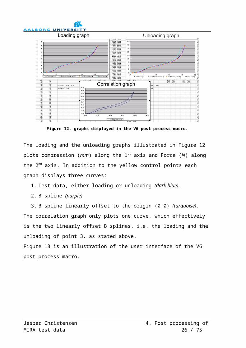
Figure 12 is and illustration of the graphs displayed in the V6 post process macro.


Figure 12, graphs displayed in the V6 post process macro.

The loading and the unloading graphs illustrated in Figure 12 plots compression (mm) along

the 1st axis and Force (N) along the 2nd axis. In addition to the yellow control points each

graph displays three curves:

1. Test data, either loading or unloading (dark blue).

2. B spline (purple).

3. B spline linearly offset to the origin (0,0) (turquoise).

The correlation graph only plots one curve, which effectively is the two linearly offset B

splines, i.e. the loading and the unloading of point 3. as stated above.

Figure 13 is an illustration of the user interface of the V6 post process macro.

Figure 13, illustration of V6 post process macro user interface.

The test data is imported into the macro by pressing the orange button, and choosing a *.xls

file. The macro will subsequently import all the test data of the *.xls in the active folder.


In Table 2, the variables used to enforce the characteristics of the V6 macro stated in Table 1

were listed. These variables are adjusted by the cells highlighted in yellow and green in

Figure 13. Once the test data has been imported by the macro, the buttons highlighted in

yellow can then be used to fit the B spline curves illustrated in Figure 12 to the test data. If a

change in the number of control points is desired, this can be done by entering the desired

number of control points in the areas highlighted in green, Figure 13, and subsequently

pressing either the button highlighted in violet or turquoise to refit the B spline with the

desired number of control points. The maximum number of control points has been set to 17,

although this number could be altered with relative ease.

Furthermore an area is highlighted in red in Figure 13. This area displays the difference in the

endpoint values, i.e. the difference of the last control point values between the loading and the

unloading curve. This is intended to serve as a basic quality check, in order to confirm that the

two B spline endpoints are coincident, thus ensuring that the correlation curve is continuous.

For further details regarding the V6 post process macro, please see Appendix C and the file:

“V6_macro_overview” enclosed on DVD 1.

The output of the V6 macro is the material data to be used for the subsequent LS-DYNA

analyses. At this point it is necessary to specify which material model is to be used. The

choice of material model has been dictated by JLR, as the one primarily used to model the

seat foam in conjunction with crash analysis, namely: *MAT_057.

Another LS-DYNA material model, *MAT _083, is sometimes also used in these types of

analyses at JLR. The implications, differences, advantages and disadvantages of using either

of the two material models will be addressed in the LS-DYNA chapter of this report. At this

particular point, only one thing needs to be underlined:

The *MAT_057 and the *MAT_083 material values are derived by using the loading values

from the MIRA tests, i.e. the unloading data is not used for this task. This may seem an odd

choice, but the reason is simple, and the choice has already been made, when choosing either

the *MAT_057 or the *MAT_083 material model for the LS-DYNA analyses. The reason is

quite simply, that the material models only takes the loading curve into account and calculates

the unloading curve based on the loading curve and other variables. This is done regardless of

whether the unloading curve data is entered or not. The variables related to the *MAT_057

material model will be further explained in chapter 6.

The loading data is to be given in table form stating engineering stress vs. engineering strain

hence this is the ultimate output of the V6 post process macro.


This obviously raises the question why have the unloading tests been conducted, and why

spend the time post processing them?

The answers to these questions are relatively simple. Firstly the overall governing task of this

project, i.e. the coalition of physical foam testing to a LS-DYNA model must be taken into

account.

Figure 14 illustrates a correlation curve, i.e. post processed force vs. compression values for

the loading and the unloading curve.

Figure 14, correlation curve for: L322-1-1-10 mm/min, specimen1.

Figure 14 clearly shows that the force vs. compression curve for the tested foam is nonlinear,

and thus so will the engineering stress vs. engineering strain curve be.

Furthermore, Figure 14 also clearly indicates that the loading and the unloading paths are not

identical, which is likely to be caused by the viscoelastic nature of the material. This justifies

the choice of testing the specimens for loading and unloading. The reason for post processing

the results is simply to be able to compare these results to the LS-DYNA model results which

will be introduced in chapter 6.

The description of the V6 macro is now complete, and the next step is to compare results

obtained by the V3 macro to those of the V6 macro.


4.4 Comparison of V3 and V6 macros

This section aims to compare the post processed results obtained by use of the V3 macro to

those of the V6 macro. As previously stated, some post processing had already been done,

before the author of this report became involved in this project. To elaborate, the post

processing of the L322 vehicle program, i.e. the Range Rover, had already been completed

with the V3 post process macro. Subsequently the post processing of the specimens chosen to

represent the characteristics of the L322 seats in the defined locations has been repeated by

use of the V6 macro in order to compare these results. Figure 15 illustrates a V3 post

processed loading curve, and Figure 16 illustrates the loading curve, but post processed using

the V6 macro.

Figure 15, V3 post processed loading curve for: L322-1-4-500 mm/min, specimen 3.

In Figure 15 and Figure 16, the dark blue line is the actual test results, the purple line is the

Cubic spline (Figure 15) or the B spline(Figure 16), the yellow dots are the control points, and

finally the turquoise line is the purple line linearly displaced to the origin of the coordinate

system.


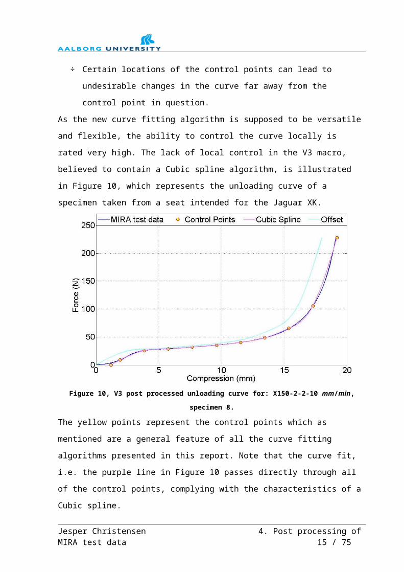
Figure 16, V6 post processed loading curve for: L322-1-4-500 mm/min, specimen 3.

The two figures show a sample that is seemingly not particularly corrupted by noise.

When comparing Figure 15 to Figure 16 for a compression value of approximately 35 mm and

above it is clear that the B spline of Figure 16 provides a better curve fit to the original test data

than the Cubic spline of the V3 macro.

The difference in force values relative to a compression values calculated by the V3 macro

and the V6 macro are somewhat cumbersome to determine, as the two macros do not specify

identical 1st axis values as reference points. Instead the two areas below the curves, i.e. the

area below the purple line of Figure 15 and the purple line of Figure 16, have been estimated

by means of numerical integration. These calculations show that in this particular case the

difference is approximately 0.9 %.

This calculation has been repeated for the remaining has been repeated for specimen 3 at the

three other test speeds of the L322-1-4 batch, and the results show an average difference

between the two areas of approximately 5.3%. The minimum difference was found to be app.

0.3% and the maximum difference was found to be app.18.7%.

These results clearly indicate that substantial differences between the two curve fitting

algorithms can be achieved, with the V6 post process macro providing results that are more

true to the original test data.

It should be noted that the end control points in Figure 15 and in Figure 16 are not coincident

with the maximum compression value of this specific test. This is due to the fact that when


either of the macros determines the end points it is based upon the largest force value, and not

the largest compression value. In the majority of the test results the largest force value

correlates to the largest compression value. This is however not the case for the given test

results illustrated in Figure 15 and Figure 16. The exact reason for this inconsistency remains

unknown; it could simply be considered as noise in the test data, it could be due to limitations

of the measuring accuracy of the test machine, it could be a consequence of the high

compression value combined with the high strain rate, it could be due to viscoelastic- or

plasticity-effects, a combination of the above, or it could be due to a completely different

reason. The fact remains that the location of the control end points throughout the post

processing phase will be based upon the largest force value.

It should also be noted that the Cubic spline of the V3 macro passes exactly through all of the

control points. This is clearly not the case of the B spline, which merely utilises the control

points to influence the resulting curve.

Figure 15 and Figure 16 does thereby confirm the claim that the B spline algorithm of the V6

post process macro would provide a better curve fit to the original test data, than that of the

supposed Cubic spline algorithm of the V3 post process macro.

Figure 17, V3 post processed unloading curve for: L322-1-4-500 mm/min, specimen 3.


The improved curve fitting ability of the V6 macro as opposed to the V3 macro is even more

obvious when regarding the unloading curves, illustrated in Figure 17 and Figure 18,

respectively.

Figure 18, V6 post processed unloading curve for: L322-1-4-500 mm/min, specimen 3.

The maximum end point of the purple curves in Figure 17 and Figure 18 does at first glance

not seem to line up with the test data. These end points are coincident with the maximum end

point values of the loading test; see Figure 15 and Figure 16, respectively. The reason for this

is to ensure that when plotting the loading and unloading curve in a force vs. compression

diagram the curve will be continuous.

At this particular point in time, the accuracy of theV6 post process macro has not been

determined, this is necessary in order to justify the results of the V6 macro.

4.5 Accuracy of V6 post process macro

The accuracy of the V3 post process macro has prior to this project been substantiated by

comparing the results of the physical testing to those of the LS-DYNA models. As the part of

the code used to import the MIRA data is identical for the two macros, this part of the V6 post

process macro can straightforwardly be substantiated.

The major difference between the two macros is as previously mentioned, the curve fitting

algorithm.


Figure 16 and Figure 18 further gives a clear visual indication of the accuracy of the V6 post

process macro, because it is clear that the B spline to a certain extend fits the original data. In

an attempt to further support the accuracy of the B spline algorithm that has been programmed

in the V6 macro one example from [Rogers, 2001] has been calculated using the B spline

algorithm of the V6 macro. This is example 3.5 pp. 67-69, which has 5 given control points

and a smoothness factor, k = 3. During this process, the following values were checked and

compared:

Individual chord lengths

Total chord length

Values of the knot vector

The values of all blending functions Ni,k(t) for k =1, 2, 3 and t = ½ and t = 2.

P(t) values for t = ½ and t = 2.

All checks listed above showed coincidence, and can thus be used to further substantiate the

accuracy of the B spline algorithm of the V6 post process macro.

The next step is to compare the *MAT_057 material data for the L322 seats obtained by the

V3 and V6 macros, respectively. Figure 19 illustrates such a comparison.

Figure 19, comparison of V3 and V6 *MAT_057 data.


Figure 19 shows overall a good correlation between the *MAT_057 values, i.e. the

engineering strain vs. the engineering stress, of the V3 and the V6 post process macros.

However, at strain values above approximately 0.75 the two curves show subtle differences.

This is an indication of the difference in the precision of the curve fit adopted by the two

macros, which can also be seen by comparing Figure 15 with Figure 16. Figure 19 is thus an

indication that the V6 macro gives slightly different results than the V3 macro, the

comparison of Figure 15 with Figure 16 indicates that the values are more accurate in relation

to the original test data. Figure 16, Figure 18 and Figure 19 does therefore indicate that the

goal of obtaining more accurate post processed data, which was used to justify the

reprogramming of the V3 macro, has been obtained. Graphs similar to Figure 19 have been

made for all the specimens in L322-1-1-10mm / min and for the remaining specimens chosen

to represent the characteristics of the L322 seats in the defined locations for CAE reference 1,

i.e. L322-1-x-x. This data and the associated graphs are enclosed in *.xls format on DVD 1in

the folder: “Comparison of V3 and V6 post process macros”. The above discussions and

arguments have all contributed towards the validation of the V6 macro.

If the B spline algorithm of the V6 macro was to be fully validated, further steps such as

performing a statistical analysis would be necessary.

The circumstantial evidence stated above is deemed sufficient for justifying the results of the

V6 post process macro for this particular application, and therefore no further steps towards

the full validation will be made.

4.6 Criteria for post processing MIRA test data

Before the actual post processing of the MIRA test data can commence, given criteria for

attempting to minimise the noise have to be set up. This includes which specimen to choose to

represent the foam characteristics of a given location. These criteria were mutually agreed

upon with Jaguar Land Rover, and are defined as follows:

1. The 1st control point of the B spline will be determined by the presence or the absence

of noise in the specific test data for engineering strain values less than 5%. The

presence of noise will be based upon the slope of the line segments that connect the

individual points recorded during the specimen testing at MIRA. If it is determined

that noise is present, the 1st control point will be dependent upon the location of the

next line segment that does not violate the specified criteria for noise. If the

coordinates of the two end points of this line segment are denoted (Pxi, Pyi) and (Pxi+1,

Pyi+1) the compression value that is equal to 5% engineering strain is denoted


P5%engs and the corresponding force value is denoted P5corrf then the criteria for

determining the value of the 1st control point, SCP coordinates can be formulated as:

2. The end control point of the B spline will be determined based upon the maximum

value of the force applied and the corresponding compression value.

3. The specimen used to represent the foam in the specific location should be a typical

specimen where the post processed data show a relatively small deviation from the

majority of the other relevant post processed specimens. This deviation is to be

understood in terms of engineering stress vs. engineering strain values. The specimen

must be an actual physical specimen, i.e. not any type of averaged specimen.

The execution of points 1 and 2 stated above will be based upon mathematical formulations,

where as point 3 will be based upon a subjective assessment.

The criteria stated above imply that additional programming is required before the actual post

processing can begin. The end control point requirement is already implemented in the V6

macro, as it does find the maximum force value and utilises this as the end control point. The

selection of the specific specimen will be further elaborated later on in this chapter, because

this selection will not be made, before the curve fitting stage has been completed. This leaves

the starting control point to be determined. As stated, the determination of this will be based

upon the slope of the lines segments connecting two adjacent points recorded during the

physical testing, below 5% engineering strain. The implementation of this “built in noise

reduction” has been carried out as described below.

Figure 20 is an example of the start of a load curve to be processed. The dots on the blue line

represent the data recorded from the physical testing. The lines in between represent the linear

line segments connecting two adjacent points. The red dot with the yellow centre represents a

control point. The red, the yellow and the orange lines indicate areas where noise has been

detected, based upon the slopes of the line segments. In this particular example, 5%

engineering strain is equal to a compression value of 1.0 mm. Please note that Figure 20 is for

illustrational purposes only.


Figure 20, example of initial load curve.

The 2nd control point of the B spline is positioned at the point of the actual test data closest to

5% engineering strain in this example this value is 1.0mm. In the case, where

The slopes of each individual line segment below this engineering strain value are

subsequently calculated. The number of points below 5% engineering strain is approximately

60, this is however not the case in the example illustrated by Figure 20, as the number of

points has been reduced for clarity.

This relatively large number of points in a relatively small interval of strain values means that

even though the slope of the individual line segment may be very low or even negative it does

not necessarily mean that the overall slope of the curve in a specified interval is very low or

negative. This can be illustrated by Figure 20, where, in general, the force values of the blue

points increase with increased compression values. However, it can also be seen that

individual line segments that have negative slopes exist. This poses a potential problem,

because the presence of a single line segment with low or negative slope may result in a larger

interval of the test data being cut off unnecessarily. In the example illustrated by Figure 20,

the 1st control point coordinates would be placed at point 2 on Figure 20. This results in all

data below this point being unnecessarily omitted from the continued correlation process.

This problem has however been overcome by considering a continuous series of line segment

slopes, and basing the assessment of whether noise is present or not upon an accumulated

slope of line segments. The determination of the 1st control point coordinates will still be

based upon equations , and . However, this moderation will in this example imply that the 1st


control point coordinates will be those of point 1 in Figure 20 and only data below this point

will be omitted.

The next step is to determine the minimum accumulated slope value that is acceptable without

adjusting the 1st control point coordinates. For this purpose, the loading graph for L322-1-1-

10 specimen 1 was chosen as being the bordering case where the accumulated slope value is

deemed acceptable. The slope of the curve, the indication of the 5% engineering stress

interval and the location of the 2nd control point are all illustrated in Figure 21.

Figure 21, close up of L322-1-1-10 spec. 1 loading curve.

The unloading graph of the L322-1-1-10 specimen 1 has an accumulated slope value less than

that of the border line curve of Figure 21, and therefore the V6 PP macro has adjusted the 1st

control point, as illustrated in Figure 22.

Figure 22, unloading curve for L322-1-1-10 spec. 1, adjusted 1st control point.

In the previously conducted post processing of the L322 series, the starting points were

manually adjusted by a subjective assessment with no clear definition to follow. These


manual adjustments are compared to the ones conducted by the V6 post process macro for 6

specimens of the L322-1 batch. The documenting for this process can be found on DVD 1 in

the folder: “Comparison of V3 and V6 post process macros”.

The built in adjustment of the 1st control point as described above is a coarse one, and further

steps could be made to refine this built in adjustment. However, a systematic approach to

adjust the 1st control point is now being used, as opposed to a manual adjustment.

Furthermore, JLR states that the material characteristics below 5% engineering strain is of

less importance, as these are very seldom used in the FEA analyses.

Therefore, the V6 post process macro is now complete and the curve fitting of the MIRA test

data can commence.

As mentioned earlier, part of the curve fitting stage of this project had previously been

completed this included the L322 and the X150 series. In addition, the task of selecting the

specimens to represent the characteristics in a specific area of a particular seat in the L322 and

X150 vehicle programs had also previously been conducted. However, due to the fact that the

curve fitting algorithm technique has changed, it is chosen to refit the curves to the previously

chosen specimens, i.e. the curve fit of the specimens in the L322 and the X150 series are

limited to specific specimens. The list of specimens can be found in the file: “PP_tracker.xls”

enclosed on DVD1. In addition to the curve fitting of these specific curves, all MIRA test

results relating to the X250, the X358, the Rowa and the Plus Pad series have been curve

fitted. All post processed files, including the V3 post processed files of the L322 and the

X150 vehicle programs can be found in the folder: “Post processed data” on DVD 1. The criterion for choosing the individual specimens to represent the characteristics of a

specific area of a particular seat has been previously stated. The actual selection of a specific

specimen is carried out, based upon a visual assessment. Figure 23 is a plot of the correlation

curves initially obtained by curve fitting the B spline of the V6 macro to MIRA test data from

the X250-1-3A-10 mm / min tests. The curves of the graph are obtained by plotting the

correlation force vs. compression curves for all the specimens with identical reference

numbers. In the case of Figure 23 the reference is: X250-1-3A-10 mm / min. In this example

specimen 4, i.e. the blue curve, was chosen as the specimen to represent the characteristics for

this specific location.


Figure 23, correlation curves for ref: X250-1-3A-10 mm / min.

In general, all test speeds and the general tendency off all the curves have been considered

when choosing a specimen, i.e. the overall shape and location of the individual curves in

relation to each other. If no distinct abnormalities, such as relatively large peak force values,

were found, the 10 mm / min test was used to select the specimens. In the case distinct

abnormalities existed, the deviations were assessed on a case by case basis, and in certain

cases the deviating curves were deselected. This was the case, if the correlation curves of the

specific specimen did not show consistency throughout the different test speeds, relative to

the general tendency of the other specimens in the batch.

A closer look at Figure 23 reveals that the peak force value of the chosen specimen, i.e.

specimen 4, is somewhat larger than the other peak force values. The lowest force peak value

of the correlation curves in question is that of specimen 1, which is approximately 0.82 times

the peak force value of specimen 4s correlation curve.

During the post processing stage, it was revealed that the difference in peak force value is a

general tendency of the test results. In fact, the factor of 0.82 found in the above case is

relatively low compared to the overall tendency. This fact substantiates one of the overall

governing problems that initially led JLR to initiate this project; namely that the material

characteristics throughout a seat foam varies greatly with location, which is highly

undesirable in relation to FEM crash analysis.


The overall object of this project it to determine 1 set of material characteristics per location

to be used in relation with FEM analyses a JLR. However, this task is obstructed by this

tendency of difference in peak force values.

In an attempt to overcome this obstacle it has been decided to allow a difference of up to 50%

in peak force values of specimens with identical references, without selecting multiple

specimens to represent the characteristics of the seat foam within that specific reference. This

criterion is set up as stated in equation below:

If the criterion in equation is violated and the specimen in question follows the overall

tendency of the other specimens with identical references as explained above, multiple

specimens were chosen to represent the material characteristics of that particular reference.

Figure 24 illustrates the correlation curves for the reference: X250-4-2A-10, which is an

example where equation is violated.

Figure 24, correlation curves for all specimens in X250-4-2A at a test speed of 10 mm / min.

From Figure 24 it is clear that the correlation curves for specimens 1 and 2 differ significantly

from those of specimen 3 and 4, despite all specimens being of similar height and diameter.

The tendency of “two general correlation curves” as illustrated in Figure 24 is consistent

throughout this particular batch. Figure 25 illustrates the correlation curves for specimens 2

and 3 from this batch, for all test speeds, where it can be seen that the correlation curves for

specimen 3 differ significantly from those of specimen 2, thereby further confirming the


acclaimed tendency. Plotting the correlation curves of specimen 1 and 4 reveal the same

tendency, however due to clarity these curves have been omitted from Figure 25.

Figure 25, correlation curves for X250-4-2A, specimens 2 and 3.

In the case above, i.e. X250-4-2A, both specimen 2 and specimen 3 have been selected to

represent the characteristics of the seat foam in this particular area. This is due to the fact that

equation has been violated, and because the correlation curves for specimen 1 and specimen

3 show relatively small differences when compared to specimen 2 and specimen 4

respectively. This indicates that the difference is not likely to be due to noise being present in

the test results.

The above example is not a unique case, in fact several batches have shown the tendency

illustrated in Figure 24 and Figure 25, these batches and further discussions as to why these

differences occur will be elaborated in the following chapter. In addition, the next chapter will

evaluate the test results, and point out some of the issues connected with the test procedure

adopted to perform the physical testing of the foam specimens.



5. Evaluation of physical testingThe purpose of this chapter is to highlight some of the weaknesses, uncertainties and errors

that were made during the physical testing of the foam specimens, in addition to evaluate the

overall test results.

The outcome is to be a general list of recommendations and suggestions that can be used as a

starting point for future testing similar to those documented by this report.

5.1 MIRA test results

In general the related test results show an overall consistency, when the criteria of equation

is applied. However, test results that violate this criterion where still found, all of which are

examined throughout this chapter.

In the introduction to this report it was revealed that not all specimens from the same batch

have similar height, which could lead to differences in correlation curves as all specimens was

to be compressed by approximately 80% of their original height. This is however not the case

in the example illustrated by Figure 24 and Figure 25, but this could be a factor in certain

cases. Table 3 lists all the cases found during the post processing stage, where equation has

been violated, and therefore two specimens have been chosen to represent the foam

characteristics of the area in question. Please note that the specimens listed in Table 3 do not

necessarily represent the actual specimens that have been chosen to represent the foam

characteristics. Instead they represent the minimum, denoted “MIN” and the maximum,

denoted “MAX”, peak force values of the correlation curves of a particular batch at a

particular test speed. Please also note that the engineering stress difference and the

engineering strain difference both have been calculated as the value of the specimen denote

“MAX” minus the value of the related specimen denoted “MIN” in Table 3. Negative values

in either of the last two columns will therefore imply that the value of the specimen denoted

“MIN” is larger than the related specimen denoted “MAX”.

Jesper Christensen5. Evaluation of physical testing 36 / 75

Table 3, batches where two specimens have been chosen for correlation.

Reference

# Peak force

Spec No.

D (mm

)

T (mm

)

Peak Force Value (N

)

Displ. C

orresp. to F (m

m)

Eng. stress diff.(Pa)

Eng. strain diff.

Peak force factor (MAX/M

IN)

L322-2-4A 10 mm/min

MAX 3 49.4 25.6 80.8 19 21275.6 0.04 2.25MIN 2 46.8 26.8 35.92 18.83

L322-3-6 10 mm/min

MAX 2 49.1 23.9 82.3 17.32 18461.2 -0.03 1.68

MIN 3 49.9 23.1 48.9 17.42L322-4-4A 10 mm/min

MAX 6 48.6 48.8 64.58 39 16810.6 0.05 1.99MIN 12 47.9 24.2 32.44 18.12

X150-2-4A 10 mm/min

MAX 4 51.3 24.6 119.38 18.7 17475.1 -0.04 1.54

MIN 6 49.5 23.5 77.52 18.8X150-4-2A 10 mm/min

MAX 5 48.9 23.5 156.6 17.9 48495.1 -0.04 2.35

MIN 2 49.3 22.4 66.6 17.9X250-4-2A 10 mm/min

MAX 3 50.2 12.9 22.25 9.78 -37666.1 0.09 0.24

MIN 1 49.6 15.4 94.5 10.3X358-1-4

500 mm/minMAX 10 50 24.9 194 18.08 69108.2 0.00 3.19MIN 1 51.1 25 60.9 18.1

X358-1A-2 10 mm/min

MAX 1 49.5 26.3 84.9 19.5 18317.2 -0.01 1.71

MIN 2 49.5 26 49.65 19.56X358-2-1

100 mm/minMAX 4 49.9 50.4 172 37.04 52568.6 0.11 2.47MIN 3 50.1 51.2 69.75 32.02

X358-2-2 10 mm/min

MAX 4 50 25.5 230.25 19.5 91069.5 0.03 4.49MIN 6 49.9 25 51.23 18.44

X358-4-3 10 mm/min

MAX 3 49.6 22.3 149.1 17.6 55844.6 0.03 3.66MIN 6 49.3 23.1 40.7 17.6

X358-5-1 10 mm/min

MAX 1 49.7 24.4 184.4 18.2 64377.2 0.02 3.12MIN 2 49.5 25 59.03 18.18

X358-5-1B 10 mm/min

MAX 4 49.6 24.7 144.6 17.86 48942.3 -0.03 2.93

MIN 5 49.3 23.8 49.43 17.84X358-5-2

100 mm/minMAX 3 50 24.6 169 18.26 47116.5 0.00 2.19MIN 14 50.2 24.5 77.1 18.22

In addition to Table 3, the specimens denoted in Table 4 also violates equation . Therefore, it

would seem that the material characteristics in the locations referred to in Table 4 should also

be represented by two specimens.


Table 4, specimens of batches where equation has been violated.

Reference

# Peak force

Spec No.

D (m

m)

T (mm

)

Peak Force Value (N

)

Displ. C

orresp. to F (m

m)

Eng. stress diff.(Pa)

Eng. strain diff.

Peak force factor (MAX/M

IN)

X358-1-2 100 mm/min

MAX 5 48.7 18.9 313.6 18.58 146332.5 0.24 7.52MIN 2 49.1 24.5 41.7 18.26

X250-4-1 500 mm/min

MAX 2 49.5 48.6 360 38.8 86872.8 0.05 1.86MIN 4 49.6 24.1 193.6 18.06

X250-4-1A 10 mm/min

MAX 1 48.9 49.8 1025 42.5 447913.8 0.07 5.67MIN 5 48.5 25.1 180.8 19.7

However, if the engineering stresses vs. the engineering strains for the specimens in Table 4

are plotted, it becomes clear why this is unnecessary.

Figure 26, strain vs. stress for X358-1-2 at a test speed of 100 mm / min.

Figure 26 plots the engineering stress vs. the engineering strain for X358-1-2 specimen 2 and

5, at a test speed of 100 mm / min. These two test specimens represent the highest found peak

force factor of 7.52, as denoted in Table 4. Figure 26 does however reveal that the deviation

between the two curves is relatively small. The relatively large peak force factor occurs

because specimen 2 is only compressed to a strain value of approximately 0.75, where as

specimen 5 is compressed to a strain value of approximately 0.98. This fact, substantiated by

Figure 26 makes for a strong argument as to why this relatively large peak force factor occurs.


In Table 4 it can also be seen that the thickness of the two specimens, i.e. X358-1-2, specimen

5 and specimen 2 are of significantly different height, which could be used to further explain

the peak force factor. Similar arguments could be made for the remaining four test specimens

listed in Table 4, plots of the related eng. stress vs. eng. strain curves supports the decision to

only use one specimen to model the material characteristics in these locations.

The argument relating to the different specimen heights could also be used to partly explain

the peak force factors of the specimens listed in Table 3. However, when plotting the eng.

stress vs. eng. strain for the related specimens, they show relatively large deviations from each

other, and therefore rules out the possibility of utilising one specimen to represent the material

characteristics in the area in question.

In an attempt to further explain the differences listed in Table 3 the specimens in question

were located, and it was attempted to find the precise location on the actual seat foam where

they were originally cut from. During this process, it became clear that all specimens in

question were cut from larger samples, i.e. a taller cylindrical specimen was initially cut from

the seat foam. The ends of these initial specimens have presumably been cut off due to

geometric reasons, as the end faces of these specimens would most certainly not have been

plane. The result of this is that the specimens are from different depths, in relation to the outer

surface of the original seat foam, please see Figure 27 for details.

The majority of the test specimens denoted “MAX” in Table 3 could be directly linked to

having one surface from the actual seat foam surface. On the other hand, the majority of those

specimens denoted “MIN” in Table 3 were linked to have been taken from the “inner” part of

the original seat foam, i.e. neither of the surfaces of these test specimens were from an actual

outer surface of the original seat foam. An example of this can be seen in Figure 27 below,

which illustrates X358-1-2 specimens 2 and 5 “refitted” in the actual seat foam.

Figure 27, X358-1-2 specimens 2 and 5 locations and example of “in depth location”.


The reason why it was not possible to directly link all of the test specimens in Table 3 to

either an outer surface of the original seat foam, or the inner part of the seat foam in question

is that the original seat foam where these specimens were taken from could not be found.

If any of the original seat foams, where the test specimens were cut from, are examined, it

immediately becomes clear that the foam material characteristics changes rapidly with

location. This is the case when moving upon the outer surface of the original seat foam, as

well as when moving away from the surface, i.e. in depth. In fact, there is a tendency for the

seating foam to “soften” as the overall thickness of the cross section increases. In other words,

as the depth, i.e. distance from any outer surface of the original seat foam, increases the seat

foam seems to “soften”. This tendency might suggest that that the varying material

characteristics of the seat foam could be related to the overall heat distribution during the

hardening process of the seat foam manufacturing. However due to the overall purpose of this

report, this train of thought is not further pursued.

5.2 Strain values

The focus of attention is now returned to the issue of varying engineering strain values as

illustrated by Figure 26. The fact that specimen 2 in this case only has been compressed to a

strain value of 0.75 is not a unique example, as several cases have been discovered where the

maximum strain value is significantly below 0.8. If the MIRA test result files are scrutinised it

appears that the height of a random specimen of the batch has been utilised to calculate the

compression value corresponding to a strain value of 0.8 for that particular batch. In some

cases neither of the heights of any specimen in the batch divided by the maximum

compression value from the test data equals a strain value of 0.8. The implications of this

approach seemingly has a direct influence upon the test results, because if the height of a

given specimen is particularly lower than that used to calculate the 80% strain, then the test

data will show compression, but the force applied will be very low. This can be interpreted as

the “noise” which the V6 post process macro was programmed to cut out of the test results.

This effectively means that the actual strain value for the individual test specimen varies

greatly. The lowest strain value found is for X358-1-2 specimen 1, where the strain value is

0.68. The maximum strain value that has been found is the one stated above, namely 0.98.

The specifications dictated by JLR before the test stated that all specimens must be

compressed to a maximum strain value of 0.8. The calculations above clearly show that this

test specification has not been met. The fact that the specimens have been compressed in

excess of 80% strain is of less importance, as the value of the engineering stress at a strain


value of 0.8 can still be found from the data supplied by the test. This is off course not the

case when a strain value of 0.8 has not been reached during the testing. This poses a serious

issue that greatly influences the results of the correlation process, as the majority of the test

specimens seem to “stiffen up”, i.e. the slope of the engineering stress vs. engineering strain

curve increases as the engineering strain increases, examples of which can be seen in Figure

24 and Figure 25. This issue need to be addressed and corrected for future testing. However,

for the time being it is not possible to retest these specimens, and even though cases exist

where the strain value is less than 0.8, these results will still be used in the continued

correlation process.

5.3 Load cell

As stated in the introduction, the load cell used for the physical testing was 1000 N.

MIRA has been contacted, in order to receive information regarding the compression test

machine, the load cell used to conduct the testing of the foam featured in this report and

general guidelines for physical testing.

The 1st question given to MIRA is regarding load cells used for compression testing.

The question was formulated as:

What is the percentage of a load cell value under which they should not be used?

The answer listed below is a direct answer from MIRA, the email which was sent can be

found enclosed on DVD 1 in the file “MIRA information regarding test facilities.doc”:

“They are calibrated between 1% and 100%, but it is not recommended to use any load cell

below 5% of scale due to resolution etc. If you consistently operate below 5%, then get a

smaller load cell! It is good practice to ensure your UTS is within 25% to 75% of your load

cell”

As 5% of 1000 N is 50 N, the question can be raised as to why a 1000 N load cell has been

used when many of the conducted measurements lie beneath 50 N. A glance at Table 3 and

Table 4 reveals that approximately 30% of the peak force values listed are below or in the

immediate vicinity of 50 N. It is therefore likely that the choice of load cell has had an

influence on the test results, although the scale of this influence remains unknown. However,

the lower calibration value should, according to MIRA be 10 N, thereby somewhat

confirming the accuracy of the test results. One thing is for certain, the “good practice” as

stated in the MIRA answer has not been met in this case, assuming that these values are the

identical for compression as well as tensile testing.


Figure 8, page 9 in chapter 3 is a picture of the actual MIRA test setup.

The picture reveals that a long rod connects the compression test machine to the plate that is

in direct contact with the actual test specimen. Depending on the straightness of this long rod,

the presence of it could contribute to the force applied to the test specimen being at a different

angle than 90 degrees relative to the top surface of the cylindrical test specimen. Furthermore,

the presence of the long rod implies that the force measured during testing is measured at a

relatively large distance from where the test specimen is located, and thus part of the measure

force could contribute to the compression / bending of the long rod during testing. If the rod is

assumed to be made from aluminium with a Young’s modulus of 70 GPa, and the stiffness of

a typical foam test specimen is estimated from the initial slope of the engineering stress vs.

strain curve, to be 10 MPa, it is highly unlikely that the compression/bending of the rod will

have a significant influence on the actual test data. Nevertheless, the fact remains that the

presence of the long rod is a contributing factor to the uncertainty of the tests conducted.

5.4 Test specimens

The focus of this chapter now shifts to the actual foam specimens.

As previously stated, the foam test specimens were chosen to be cylindrical in an attempt to

minimise shape effects. However, as the specimens are cut out of actual seats, the end

surfaces of the cylindrical test specimens are not necessarily parallel.

Figure 28 illustrates a typical example of a specimen where the ends of the test specimen are

unparallel, the volume of this specimen is approximately mm3, and is thus

representative of the majority of specimens with an approximate diameter of 50 mm and an

approximate height of 50 mm.

Figure 28, example of non parallel ends, X250-4-1, specimen 3.

The fact that the height of the specific specimen is not constant, as the ends are not parallel

means that the height of the individual specimen can not be uniquely determined. In addition,

the consequences of the unparallel ends could mean that initially, lower force values would be


measured during testing, opposed to a specimen where the ends are more parallel than the

specimen illustrated in Figure 28. This possibility could also contribute to the presence of

noise in the test data, as discussed in chapter 3 and illustrated by Figure 9, page 10.

A way of overcoming this problem could be to cut the foam specimens in such a way that the

ends of the individual specimens would be more parallel. However, this approach has

apparently been applied to some of the test specimens, resulting in specimens from varying

depths as previously discussed. An alternative way of attempting to minimise this problem

could be to initially introduce a given strain value before commencing the actual

measurements. In connection with the previous discussion regarding the presence of noise in

the test data, it was stated that the values below 5% strain is of negligible interest in relation to

FEA analyses. Therefore, a possible solution to the problem of the unparallel ends could be to

subject the specimens to a strain value of 0.05, in relation to the maximum height, see Figure

28, of the test specimen, and setting this as the starting point for the test.

The net section of this chapter is solely related to the Plus Pad results.

5.5 Plus Pad results

This section is solely concerned with the Plus Pad test results. It explains why the Plus Pad

results have been omitted for the remainder of the correlation process.

Figure 29 is an illustration of the 6 mm Plus Pad results for specimen 1.

Figure 29, 6 mm Plus Pad results specimen 1.

All curves on Figure 29 show a “hump” on the correlation curve in the region of 0.5 mm to

1.0 mm compression value. The presence of these “humps” can be used to question the

accuracy of the test results for this foam specimen.


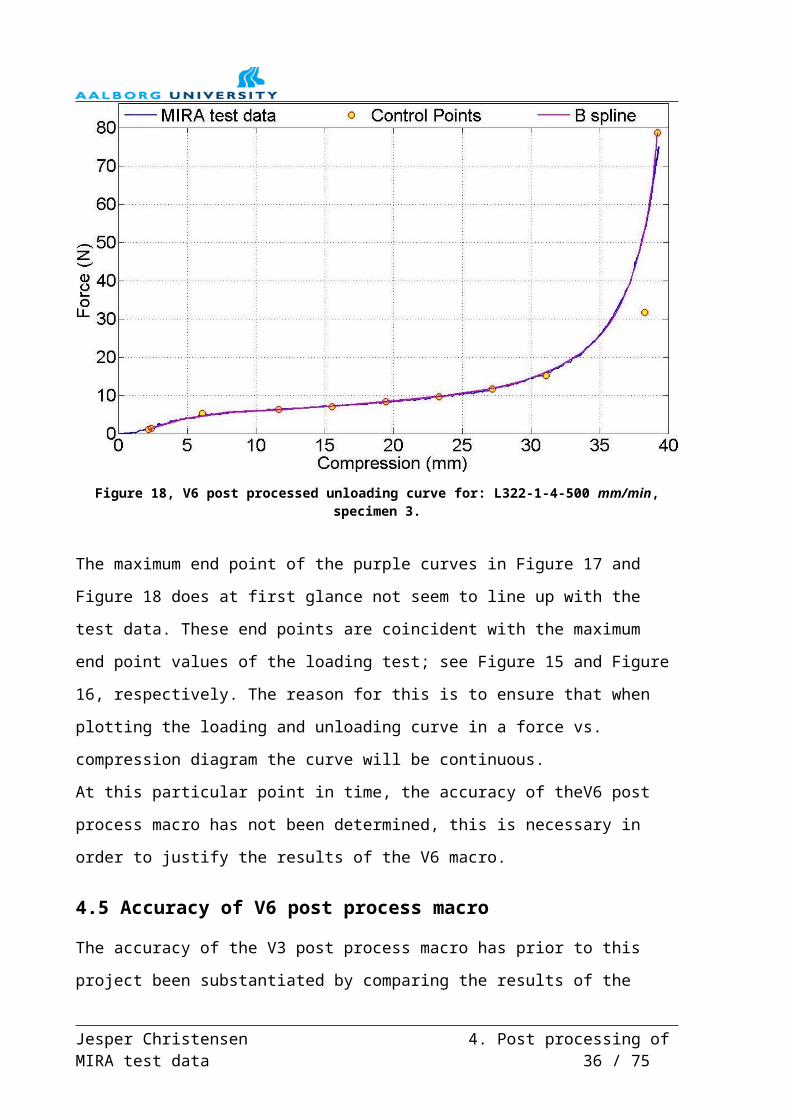
All the 6 mm plus pad specimens for a test speed of 10 mm / min are plotted in Figure 30.

Figure 30, 6 mm plus pad correlation curves, test speed 10 mm / min.

A close look at Figure 30 reveals that all the correlation curves show relatively small

deviations in relation to each other. This fact could be interpreted as the material

characteristics of all the test specimens being very similar.

However, due to the fact that all curves in Figure 29 and in Figure 30 display a “hump” in the

region of 0.5 mm to 1.0 mm compression could suggest that what has been measured is in fact

a form of inertial effects in the compression test machine. This claim can be further

substantiated by plotting all the correlation curves for the 6 mm plus pad, which also reveals

very similar results combined with the “hump” in the 0.5-1 mm compression interval. The

overall tendency is repeated when plotting the correlation curves for the 10 mm Plus Pad

specimens.

The reason for these why these tendencies occur could be found in the dimensions of the

specimens, which have a height of 6 mm. At a test speed of 500 mm / min, the time to achieve

a strain value of 0.8 is 0.58 s. Information from MIRA dictates that an average acceleration

time for the compression test machine to achieve a steady speed is 0.1 sec, which is

approximately 17 % of the test time, for either loading or unloading.

Furthermore, the “humps” illustrated in Figure 29 and in Figure 30 all occur in the vicinity of

a force of 10 N, which according to information supplied by MIRA is the lower value for

which a 1000 N load cell, such as the one used in the testing, is calibrated for.

For these reason, all the Plus Pad and the Rowa 6 mm test results, all of which display the

tendencies as described above, are deemed as unusable, and are therefore not used throughout

the remainder of this report.


In chapter 3 it was also stated that in an attempt to avoid viscoelastic effects interfering in the

test results, the specimens were allowed to rest in between tests at different speeds. No checks

were made to see whether the specimens had actually changed heights. This could simply be

done by re-measuring the heights of the individual specimens, and used as a method of

detecting the presence or absence of viscoelastic effects.

Based on the above discussion regarding the accuracy of the results from the MIRA testing of

the Plus Pads, these have been omitted from the remainder of the correlation process.

5.6 Recommendations for future testing

Based upon the discussions of this chapter, the following recommendations are given, which

are intended to serve as guidelines for similar future testing.

Attempt to create cylindrical test specimens, thereby minimising shape effects.

Attempt to create test specimens of identical height.

Attempt to create test specimens that represent the entire cross sectional area, i.e.

stride to cut the test specimens from outer surface to outer surface of the original seat

foam, see Figure 27.

Viscoelasticity, re-measure test specimens between testing to suggest the presence or

absence.

Ensure a strain value of 0.8 is achieved for all individual test specimens, provided 0.8

is the target strain value.

Choose correct size load cell, i.e. typical load values should all exceed 5% of the max

load cell value.

Attempt to avoid a long rod in the test setup.

Place load cell as close to the test specimen as possible.

Stride to make the ends of the cylindrical test specimen parallel in order to minimise

noise in the test data.

Alternatively, apply 5% strain, relative to the maximum specimen height, see Figure

28, before starting the test.

Make sure that the time before the test machine reaches a constant velocity is

negligible compared to the overall test time.


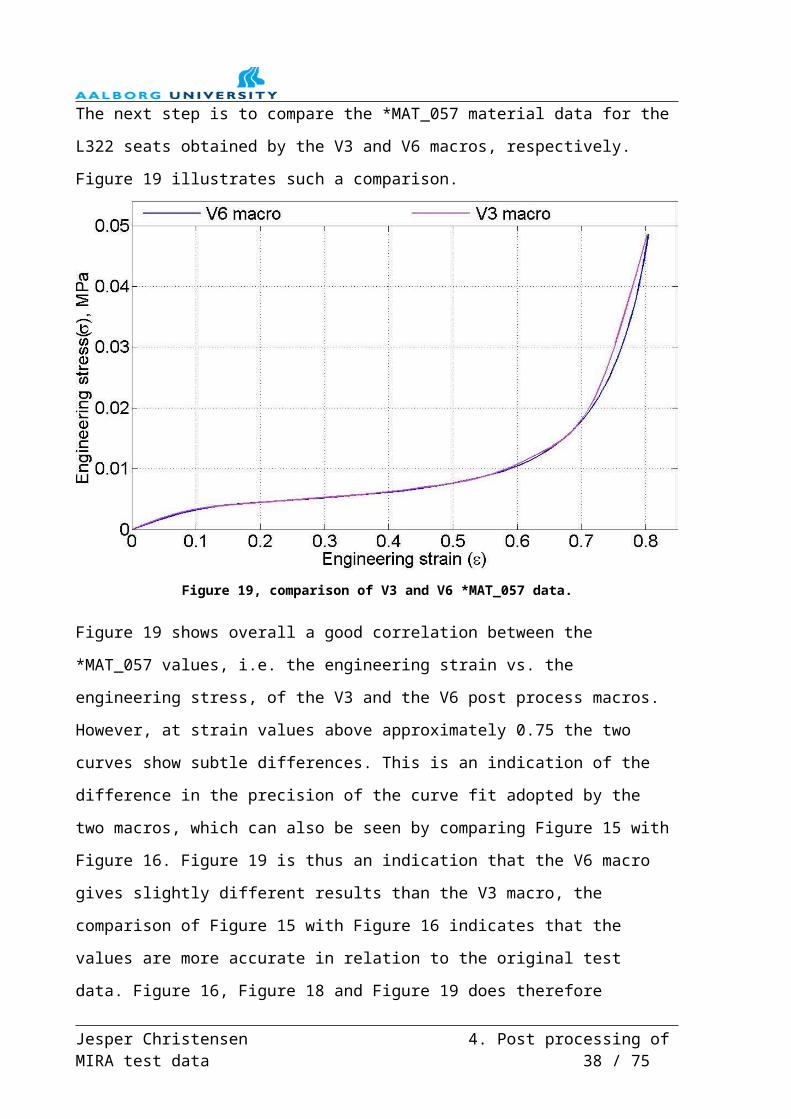
Jesper Christensen 46 / 75

6. LS-DYNA 971 keyword FEM correlation The purpose of this chapter is to document the correlation process of the physical testing

results presented in chapter 4.

The chapter will commence with a description of the actual FEM model and a thorough

explanation of the material model parameters used in the correlation process. Thereafter, the

methodology used in the actual FEM correlation process will be explained.

Throughout the entire FEM correlation process the single precision “MPP Single 971 R 3.1”

has been used, unless otherwise stated. It should also be noted that the engineering stress

referred to throughout the correlation process are σzz stresses unless otherwise stated.

An illustration of the FEM model used in the correlation process can be seen in Figure 31.

Figure 31, illustration of LS-DYNA model.

The model depicted in Figure 31 consists of five components; stem part (1), upper platform

(2), foam specimen (3), lower platform (4), spring (5) and damper (6).

6.1 General FEM model description

The spring and the damper, i.e. components 5 and 6 are connected in parallel. The lower end

point of these, i.e. the endpoint with the lowest z-value is rigidly connected to the stem part.

The end point with the higher z-value is rigidly clamped. The stem part, i.e. part 1, is rigidly

connected to the upper platform, part 2. These two combined components have 1 DOF,

namely in the z-direction, as they will initially compress the foam specimen, i.e. component 3.

Jesper Christensen 6. LS-DYNA 971 keyword FEM correlation 46 / 75

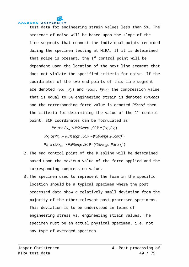
The interface between components 2 / 3 and the interface between components 3 / 4 are

modelled as contact surfaces. The lower platform is rigidly clamped.

In the dynamic analyses part 2 and part 3 will move along the global z-axis defined in Figure

31 initially loading, i.e. compressing, and subsequently unloading, uncompressing the foam

specimen.

Components 1, 2 and 4

It is desirable to reduce the influence of components 1, 2 and 4 on the analyses results, in

terms of strain and deformation energy,. Therefore, the material models of these three

components have all been set to the LS-DYNA keyword 971 material: *MAT_20: Rigid,

which models the individual component as a rigid body. The validity of this choice was

substantiated in chapter 5 , which found the stiffness of the foam specimen, part 3 in Figure

31, in relation to the stiffness of the stem part to be negligible.

The *MAT_20 material model requires three inputs; Young’s modulus, Poisson’s ratio and

the mass density. Young’s modulus and Poisson’s ratio are in this case solely used in relation

to contacting surfaces. In chapter 5, the stem part was assumed to be made from aluminium,

therefore the Young’s modulus, Poisson’s ratio and the mass density have for all three

components in question, been set to 70GPa, 0.3 and 2700 kg/m3, respectively.

Components 5 and 6

The justification for implementing component number 5, the spring, is quite simply

convenience. A spring is defined as a discrete element which can be used to directly extract

the force data during the analysis. This is less computational heavy than extracting the data

from the solid elements used to model component number 3, the foam specimen. The

combined force transferred through component number 5 and 6 will be identical to that

exerted on component number 3, because component 2 and 4 are modelled as rigids. The

justification for implementing component number 6, the damper is to damp out oscillations of

components 1 and 2 during the analysis.

During the analyses, the z-displacement of node no. 102102, see Figure 31, along with the

force in the spring and the force in the damper will be recorded. This data will subsequently

be used to plot the engineering stress vs. the engineering strain curves, which are to be

compared to the post processed curves presented in chapter 4. In order to avoid oscillations on

the force vs. displacement curve, due to the spring, during the analyses, the stiffness of the

spring has been set very high; 18000 N/mm as it is estimated that this value is adequately high

compared to the forces transferred by the spring during the analysis. The damping constant is


not as straightforward to set. The value used in the analyses has been set to 0.25 N*s/mm, and

was found by means of trial and error. The process leading to the establishment of the

damping constant value will be documented later on in this chapter, once the overall model

description is complete.

Component 3

This component models the actual foam specimen, and therefore the geometric dimensions,

i.e. diameter and thickness, will vary from analysis to analysis. In addition, the z-position of

components 1 and 2 are adjusted correspondingly for each individual analysis. The choice of

the LS-DYNA keyword 971 material model used for component 3 is very important, as the

entire purpose of the correlation process is to find the input values for such a material model

that can be used for e.g. FEM crash analysis. In general, Jaguar Land Rover utilises two LS-

DYNA keyword 971 material models for FEM crash analyses to model the seats; namely:

*MAT_057: Low density foam

*MAT_083: Mat Fu Chang Foam

The LS-DYNA keyword 971 manual describes *MAT_057 as being: Low density foam with

high compressibility, and *MAT_083 as being: Low and medium density foam with rate

effects. The difference between the two material models is not immediately clear as both, in

theory, are able to model the same material behaviour / characteristics. One of the differences

between the two is that where *MAT_057 utilises linear viscoelasticity and a convolution

integral to account for rate effects, *MAT_083 utilises a curve for the nominal stress vs.

engineering strain to account for rate effects. Both materials allow for a nominal stress vs.

strain loading input to represent the characteristics. However, in the *MAT_057 material

description it is also stated that one of the main applications for this material model is seat

cushions. Furthermore, *MAT_057 is by far the most used material model in relation to seat

foam modelling at JLR. One of the reasons for this is a lack of experience using *MAT_083.

For the reasons stated above, the FEM part of the correlation process, documented by this

report, will utilise the *MAT_057 material model. Once the correlation process is complete,

the differences between the *MAT_057 and the *MAT_083 material models will be further

examined, see chapter 7.

The *MAT_057 variables that have been used for the correlation process are:

Material density, this value has been estimated by calculating an average mass

density based upon several test specimen dimensions and weight. The value was found

to be: 54 kg/m3, and is fixed for all models.


Young’s modulus, this value was, as previously described, found by estimating an

average value of the initial slope of the engineering stress vs. engineering strain curves

from the test results. The value has been set to 10 MPa, and is fixed for all

models.

Hysteretic unloading factor, this variable influences the energy dissipation during

unloading. It can assume any value between 0 and 1. Per default, this value is set to 0,

i.e. no energy dissipation.

Shape factor, this variable also influences the energy dissipation during unloading. It

becomes active when the hysteretic unloading factor is nonzero.

As stated above, the hysteretic unloading factor and the shape factor can both be used to

adjust the energy dissipation during unloading, i.e. be used to correlate the unloading curves.

However, it was chosen to fix the value of the hysteretic unloading factor, and subsequently

conduct the correlation process solely by adjusting the shape factor. The main reason for this

decision was primarily due to the fact that the shape factor has a larger influence on the

energy dissipation than the hysteretic unloading factor, [LS-DYNA, 2009, page 1598].

Therefore, the hysteretic unloading factor was set to 0.01.

The final input for the *MAT_057 material model is a loading curve, plotting engineering

stress vs. engineering strain. This curve will vary from one model to the next. The load curves

used for this have been generated using an Excel macro that can be found in the Excel file:

PP_tracker that can be found on DVD 1.

The individual load curves are not explicitly enclosed, but can be found embedded within the

specific *.key file, which are all enclosed on DVD 1, 2 and 3.

Choice of elements

Components 1, 2 and 4 have all been meshed using the solid element: 1 constant stress,

element formulation 1”. This element formulation is the default, and assumes constant stress

throughout the element. As previously described, these components have been modelled as

rigids, and will therefore not distort nor deform during the analyses. In order to comply with

the normal procedure at JLR, component 3 has been meshed with the LS-DYNA keyword 971

solid element: “1 point tetrahedral, element formulation 10”, as these are commonly used to

model the seat foam in other FEA analyses at JLR. This particular element is a 4 node

tetrahedron with linear displacement functions and single point, i.e. reduced, integration. The

element size has been chosen by conducting a mesh convergence study based upon the

convergence criterion: Maximum compression σzz value of component 3, see Figure 31 for


definition of z axis. In addition, the time required to solve the individual models were

considered when conducting the convergence study. The values obtained during the

convergence study are listed in Table 5.Table 5, results of convergence study.

Mesh size (mm)

Number of elements

Max. comp. σzz value (Pa)

Approximate solver time (min)

3.0 8178 42400 454.0 4050 41700 95.0 2635 41400 6.56.0 1442 42100 48.0 402 380 1.5

Based upon the results of the convergence study, it was chosen to set the mesh size of

component 3 to 4.0mm.

Simulation time

The physical testing attempted to run the tests at a constant test speed of either 10, 100 250 or

500 mm/minute. In the FEM models the loading time, i.e. the time from zero to the maximum

displacement value, has been set to 0.4s and so the unloading time. The displacement is

measured as the z-displacement of node 102102, see Figure 31. The maximum displacement

value will be adjusted according to the maximum displacement recorded during the physical

testing of the specimen in question.

It should be noted, that due to the fact that the maximum displacement of a given specimen

was not necessarily identical for all test speeds, the maximum displacement value of the given

FEM models has been set equal to the largest numerical value of the four individual

maximum displacements. For example if the 10, 100 and 250 mm/min physical tests recorded

a maximum displacement of 0.9 mm, while the 500 mm/min test recorded a maximum

displacement of 1.0 mm, then the maximum displacement of the four FEM models in question

will be 1.0 mm.

As previously stated, it was the intention that the physical testing should be conducted at a

constant test speed. For the same reason, and in attempt to avoid relatively large force

oscillations in the test results, caused by accelerating masses at the start of the simulation,

components 1 and 2 of the individual model was given an initial velocity calculated as stated

in equation :


Sampling frequency

The sampling frequency is the remaining value to be set before the general model description

is complete. This was set equal to the sampling frequency of the load cell used for the

physical testing, i.e. 100Hz.

6.2 Determination of damping constant

As previously stated, the value of the damping constant was found by means of trial and error.

This was simply done by changing the damping constant for four otherwise completely

identical models. The model chosen was the L322-1-1 10 mm/min.

The four different damping constant values were 0, 0.25, 2.5, and 5 (N∙s)/mm.

The force vs. compression graphs indicating the influence of the damping constants are

illustrated in Figure 32.

Figure 32, force vs. compression, various damping constants.

The red curves in the graphs of Figure 32 are the FEM models results for the respective

damping constants. The green curves are all identical, and depict the force vs. compression

curves from the physical testing of this particular specimen.


Figure 32 clearly indicates that the FEM model with a damping constant of 0.25 N*s/mm is

least “noisy” of the six depicted. Therefore, the damping factor for all the FEM models has

been set to 0.25 N*s/mm.

The correlation process has subsequently been carried out on all 600 FEM models, solely by

adjusting the shape factor. The *.key files used for the analyses along with the associated

solution data can all be accessed on the enclosed DVD 1, 2, 3 and 4.

6.3 Correlation results

The purpose of this section is to evaluate the overall correlation results.

The correlation results from all 600 FEM models can be accessed from the html file:

Correlation_results.html enclosed on DVD 1. Please note that this file is intended to be

opened using internet explorer browser and a screen resolution of 1280 times 1024 pixels, in

order to display the associated files correctly. An example of the correlation result files that

can be found using the above mentioned html file is illustrated in Figure 33.

Figure 33, example of correlation result file.

As it can be seen in Figure 33, the individual file contains the model ID, specimen

dimensions, maximum values, *MAT_057 values, the spring stiffness, the damping factor and

the solver information output from LS-DYNA, as well as the correlation curves plotting force

vs. compression. The green curves always represent the results of the post processed MIRA

test data. These curves have been extracted by use of the Excel macro that can be found in the


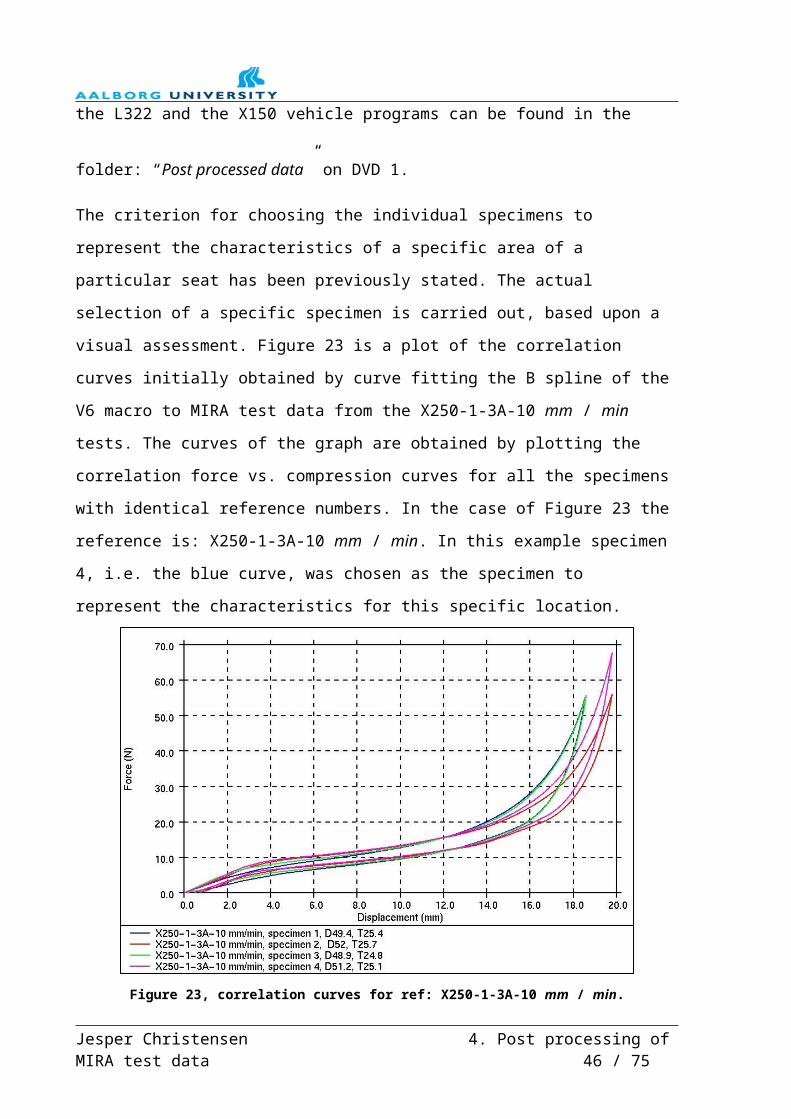
Excel file: PP_tracker and the V6 post processed excel files on DVD 1. The red curves

always represent the results of the FEM analyses. This curve has been created based upon the

output data of the individual FEM analysis, the program T/HIS and the FAST/TCF macro:

“Post_process.inp” which can also be found on DVD 1. The correlation results files have

been generated by use of OASYS93 reporter, which can be programmed to extract the solver

information displayed. The remaining data has been extracted from the *.key files via shell

scripting. This script is enclosed on DVD 1 in the folder: Scripting.

In general, the curves extracted from the FEM analyses show a good correlation with the

corresponding curves extracted from the MIRA data. However, this is not always the case, as

illustrated by Figure 34, which represents the X250-1-5A 10mm/min correlation curves.

Figure 34, correlation curves for X250-1-5A 10mm/min.

From Figure 34 it can be seen that the red FEM correlation curve is subjected to oscillations

which were intended to be reduced by the introduction of the damper, however this fact is

ignored for the time being. It can also be seen that the unloading part of the FEM curve is

above the green physical test correlation curve, for compression in excess of 14.0 mm. In

addition, it can also be seen that the unloading part of the red FEM correlation curve is below

the green physical testing correlation curve in the compression interval of approximately 2.0

mm to 12.0 mm. It might be possible to achieve better correlation by adjusting the damping

constant and the hysteretic unloading factor in this particular case. These possibilities will not

be addressed at this point in time, as the limitations of the *MAT_057 material model will be


analysed in the following chapter. The loading part of the red FEM correlation curve still

follows the green physical test correlation curve closely. Therefore the energy dissipation for

the green physical test correlation curve and the red FEM correlation curve has been

estimated in order to compare the difference in energy dissipation for this particular case. This

has been done by numerical integration using MatLab. The MatLab code can be found in the

file: “Energycalc.m” enclosed on DVD 1. In the case illustrated by Figure 34 it was found that

the area bounded by the red FEM correlation curve, i.e. the dissipated energy is less than 1%

different than the green physical test correlation curve.

As previously explained only one maximum displacement value has been set per one

specimen for all test speeds in the FEM analyses. During the physical testing at MIRA there

was not a consistent maximum displacement value for one specimen for all test speeds. These

facts will inevitably lead to differences in energy dissipation between the post processed

MIRA data and the FEM models. It has been attempted to minimise the effect of this

difference by adjusting the integration borders according to the maximum displacement value

of either the MIRA or the FEM curve. On this basis the calculations of the percent wise

difference should only be considered as an estimate. These calculations have been carried out

for all 600 specimens. The average difference between the FEM correlation curves and the

post processed MIRA curves has been found to be approximately 12%, which is deemed as

acceptable. The numerical integration results of the individual specimens can be found in the

file: Energydifference.xls which is enclosed on DVD 1.

The focus will now shift upon exploring the differences between the *MAT_057 material

model and the alternative *MAT_083 material models.


7. *MAT_057 - *MAT_083In addition to comparing parts of the two LS-DYNA keyword 971 material models

*MAT_057 and *MAT_083, this chapter will analyse some of the possible pitfalls that may

be encountered when attempting to use the previously found material for modelling seat

foams in relation to e.g. FEA crash analysis. The chapter will consist of two main topics;

namely a theoretical comparison and a comparison based upon FEM model results.

Before comparing these FEM models, the next section will briefly highlight some of the basic

differences between the *MAT_057 and the *MAT_083 material models, that are considered

relevant in relation to this project. Throughout the FEM part of the correlation process as

described in chapter 6, the single precision “MPP Single 971 R3.1” solver has been used.

However, as some of the FEM models in this chapter only have 1 element, it is not possible to

use the above solver. In addition the FEM models are not considered to be computational

heavy, therefore the double precision “SMP Double 971 SR3.1” solver has been used for the

FEM models in this chapter, unless otherwise stated.

7.1 Theoretical comparison

The LS-DYNA 971 keyword manual describes *MAT_057 as being: Low density foam with

high compressibility, and *MAT_083 as being: Low and medium density foam with rate

effects. The difference between the two material models is not immediately clear as both, in

theory, are able to model the same material behaviour / characteristics, i.e. low density foams.

A clear definition of what constitutes low density foam is not at hand and therefore this must

be evaluated on a case by case basis. Table 6 lists some of the basic differences between the

two material models that are considered relevant in relation to this project.Table 6, basic differences between *MAT_057 and *MAT_083.

Characteristic *MAT_057 *MAT_083

Man

dato

ry

Define stress/strain relationship

(compression)

Only 1 curve can be defined, must be engineering stress vs. engineering strain

Minimum of 2 curves required, strain rates must be defined (choice of engineering or true)Defining material constants

Energy dissipation (i.e. shape of

unloading curve)Controllable: Hysteretic unloading factor (HU) and shape factor (SF)

3 different options are available, see explanation below

Rate effectsAccounted for through linear viscoelasticity, variables: Young’s relaxation modulus(Ed) and the decay constant(β1)

Accounted for via interpolation between the defined stress vs. strain curves (if defined), also variable via Young’s relaxation modulus (Ed)

Jesper Christensen 7. *MAT_057 - *MAT_083 55 / 75

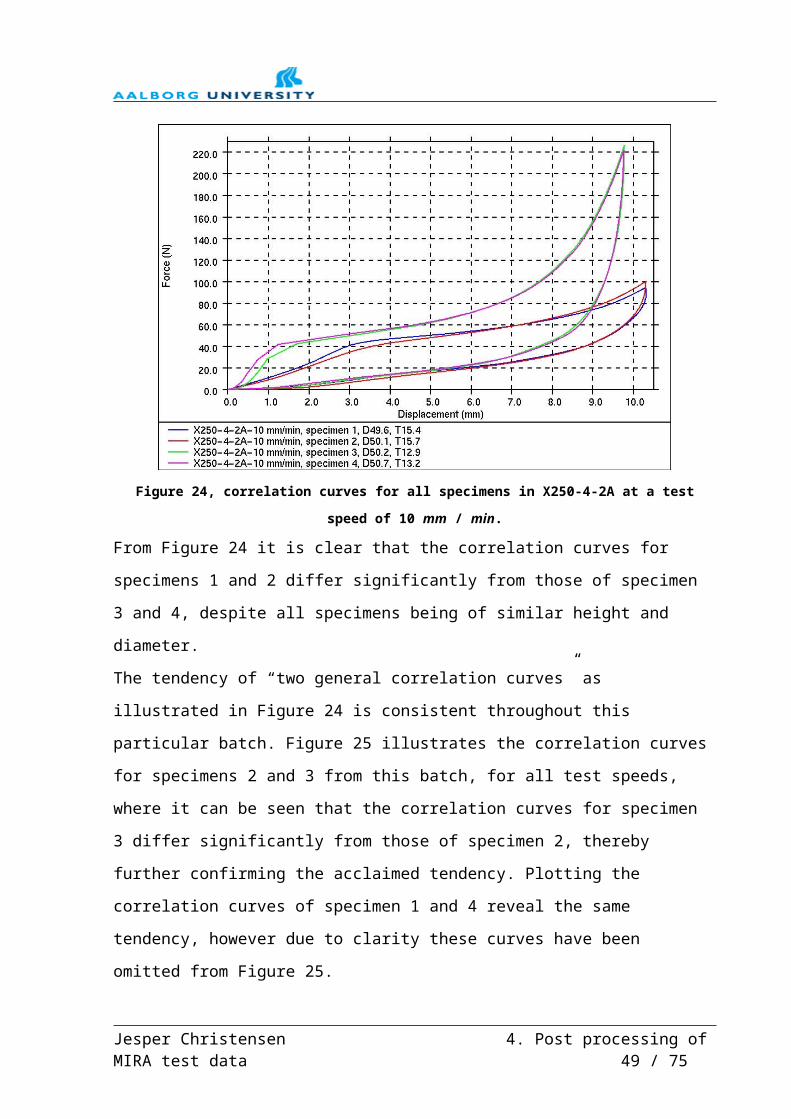
Throughout this report the option to input loading curves into the *MAT_083 material model

has been used. The curves are in this case engineering stress vs. engineering strain and the

associated strain rates are defined as engineering strain rates. The option of defining the stress

vs. strain behaviour in compression through defining material constants has not been further

explored.

Energy dissipation

As listed in Table 8, and used throughout the correlation process of this report, the

*MAT_057 material model uses the hysteretic unloading factor (HU) and the shape factor

(SF) to control the shape of the unloading curve. However, it has not been possible to obtain a

mathematical expression that shows how these variables are incorporated into the *MAT_057

material model.

Table 8 also states that three different methods of controlling the energy dissipation during a

loading / unloading cycle of the *MAT_083 material model are available. These three

methods are defined by: the variables HU and the Table ID (TBID). TBID is the table ID

which lists the individual loading curves (strain vs. stress) and the corresponding strain rates.

The options are:

1. HU = 0 and TBID < 0

This option assumes that the unloading curve is not strain rate dependent, and the

unloading curve will subsequently follow the curve with the lowest strain rate value

listed in TBID, which should correspond to the loading curve for quasi-static

loading.

2. HU = 0 and TBID > 0

This option calculates the unloading curve based upon a damage formulation for the

principal stresses, the unloading curve is therefore strain rate dependent. For this

option to be used, the curve with the lowest strain rate value in TBID must

correspond to the loading curve for quasi-static loading.

The damage formulation for the principle stresses, σi, is:

The LS-DYNA 971 keyword manual states:

“The damage parameter d is computed internally in such a way that the unloading

path under uniaxial tension and compression is fitted exactly in the formulation”


3. HU > 0 and TBID > 0

This option does not require any unloading path to be defined. The unloading curve

is calculated based upon a damage factor for the principal stresses, as was the case

with option 2, and is therefore also strain rate dependent. However, in this case, the

damage formulation is based upon the hysteretic unloading factor (HU), the shape

factor (SF) and the current value of hyperelastic energy per unit undeformed

volume. This option also specifies that the curve with the lowest strain rate value

should correspond to a quasi-static test.

The damage formulation as a function of the damage factor d, for the principle stress

σi is calculated as defined in equation .

In equation Wcur is the current value and Wmax is the maximum value of hyperelastic energy

per undeformed volume. By observing equation , it can be seen that the HU value must be less

than one in order to impose energy dissipation on the FEM model in question, and according

to the criteria for using the above damage formulation it must be larger than zero. The

boundary values of the shape factor can not immediately be determined.

Throughout this report, option 3 has been used for adjusting the unloading curve of the

*MAT_083 material models, unless otherwise stated.

Rate effects

As specified in Table 8, the *MAT_057 material model utilises linear viscoelasticity to

account for rate effects by means of a convolution integral which includes a relaxation

function. The convolution integral is as defined in equation

[LS-DYNA, 2009, page 1598]

Where is the stress tensor and gijkl is the relaxation function.

In the case of the *MAT_057 material model the relaxation function is represented by one

term from the Prony series and the relaxation function, g(t), is in this case defined as stated in

equation [LS-DYNA, 2009, page 1598].


Equation above reveals that if Young’s relaxation modulus is set to zero there will be no rate

effects, as equation will become zero. According to the LS-DYNA keyword 971 manual,

[LS-DYNA, 2009, page 1598]:

“This model is effectively a Maxwell fluid which consists of a spring and damper in series. We

characterize this in the input by a Young’s modulus , Ed, and decay constant, β1”

Table 8 lists that rate effects in the *MAT_083 material model, is accounted for via

interpolation. This claim and the consequences of altering Ed and β1 in the respective models

will be substantiated in section “7.4 Strain rate effects”.

The next section will compare FEM models utilising the *MAT_057 and the *MAT_083

material models.

7.2 *MAT_057 and *MAT_083 results comparison

The intention of this section is to compare FEM results obtained by using the two different

material models *MAT_057 and *MAT_083. In Table 6 it is stated that both of the material

models in question allow for an engineering stress vs. engineering strain curve to be used as

input. However, where the *MAT_057 model only allows one such curve per material, the

*MAT_083 model requires a minimum of two such curves, including the strain rate value of

the individual curve. The *MAT_083 material model should therefore, theoretically, allow

changes in the strain rate of the FEM model in question, without the need to change the input

engineering stress vs. engineering strain curve as is the case of the *MAT_057 material

model. The aim of this section is therefore to compare the results obtained by four individual

analyses using *MAT_057, to the results obtained by a single analysis utilising *MAT_083.

For this purpose, the FEM models L322-1-1-10, L322-1-1-100, L322-1-1-250 and L322-1-1-

500 have been selected. The only difference between these four models is the input

engineering stress vs. engineering strain curve of the respective *MAT_057 material models.

Therefore a fifth model has been created by copying one of the above models and changing

the material model for component 3, i.e. the foam specimen, to *MAT_083. The variables that

have been used for this *MAT_083 material model are listed in .Table 7, *MAT_083 variables.

Variable name ValueYoung’s Modulus 10 MPaMass Density 5.4E-11 t/mm3Hysteretic unloading factor 0.01Shape factor 0.5


The hysteretic unloading factor and the shape factor stated in Table 7 are identical to those

used for the *MAT_057 models to be compared.

The four engineering stress vs. engineering strain curves used in the individual *MAT_057

models have all been used as inputs in the *MAT_083 material model. As option 3 is used to

adjust the unloading curve of the *MAT_083 material model, the 10 mm/min curve will

therefore represent the quasi-static curve.

Table 8 below lists the equivalent engineering strain rates for the L322-1-1 models which are

used in this comparison.Table 8, equivalent engineering strain rates for L322-1-1 *MAT_057 models.

Test Speed (mm/min) Max eng. strain value, ε Eq. engineering strain rate, 10 0.808 3.584E-3

100 0.804 3.584E-2250 0.806 8.960E-2500 0.806 1.792E-1

As defined in the correlation process of chapter 6, the stem part and the upper platform part,

see Figure 31 page 46 were subjected to an initial velocity in order to avoid large oscillations

of the force vs. compression graph. This initial velocity is determined by dividing the

maximum numerical compression value by 0.4 s which is the analysis time to reach this

compression value. The time interval of 0.4 s to reach the maximum numerical compression

value has also been used for the first *MAT_083 FEM model. The maximum engineering

strain value of the *MAT_057 FEM models is 0.808, see Table 8, and the time to achieve this

value is 0.4 s, therefore the engineering strain rate of the first *MAT_083 FEM model is 2.02.

The resulting force vs. compression curve of this FEM model, and the four obtained by the

respective *MAT_057 FEM models can all be seen in Figure 35.


Figure 35, L322-1-1MAT_083 (engineering strain rate = 2.02) vs. MAT_057 results.

As it can be seen in Figure 35, the loading path of this *MAT_083 model follows the red and

the black curves, which represents the 100 mm/min and the 500 mm/min test speeds,

respectively. It is not surprising that the load curve of this *MAT_083 model with a constant

strain rate of 2.02 follows that of the 500 mm/min test, because that is the curve with the

highest engineering strain rate listed. However, it could be expected that the *MAT_083

loading curve force vs. compression values would be substantially higher than those of the

500 mm/min curve, because of the considerable increase in engineering strain rate. The reason

why this is not the case is likely, as shall be substantiated later in this chapter, is that the

*MAT_083 material model does not extrapolate strain vs. stress curves, it only interpolates.

Even though the hysteretic unloading factors and the shape factors of the respective models

are identical, the unloading curve of the *MAT_083 model seems to differ significantly from

those of the *MAT_057 models, below a compression value of 25 mm, despite the fact that

the *MAT_057 models unloading curves are similar to each other in that interval, the

difference between the two material models is therefore likely to be caused by the

implementation of the hysteretic unloading factor and the shape factor, as described in the

previous section.

Based on the analysis conducted above it is clear that the *MAT_083 material model can not

be immediately substituted with the *MAT_057 material model used in the correlation

process of this report.


The first section of this chapter took a theoretical approach to outline some of the differences

between the *MAT_057 and the *MAT_083 material models. The following sections will

adopt a practical approach to further outline some of the differences.

7.3 Practical comparison

This section will primarily be focus upon the unloading curves and rate effects.

For clarification, it has been chosen to keep the models used to further outline some of the

differences between the two material models as simple as possible. In the following

comparisons, the FEM model used will therefore be the one illustrated in Figure 36, where the

numbers represent node locations.

Figure 36, FEM model for *MAT_057 and *MAT_083 comparison.

The model consists of six tetrahedron elements, forming a cube with a side length of 10 mm.

The element formulation is identical to the one used for the foam specimens, as described in

chapter 6; namely 1 point tetrahedral, with linear displacement functions. The model will be

rigidly clamped at the 4 nodes with the lowest z value. These are denoted 5 – 8, but only three

of these are illustrated in Figure 36. During the subsequent analyses, the four nodes: 1-4,

Figure 36, are subjected to prescribed displacements in the negative z direction, with a

maximum strain value of 0.5, i.e. a maximum displacement of 5.0 mm. The general time vs.

displacement curve will be identical to that of the previously described FEM models, i.e. the

maximum displacement value will be reached after 0.4 s. The only difference between the

models that are to be compared are the material models, however the mass density of 5.4E-11

t/mm3 and the Young’s modulus of 10 MPa will be used for both material models.

Unloading curve

The purpose of this section is to examine the various options available to adjust the unloading

paths of the *MAT_057 and the *MAT_083 material models. In order to do this the linear

engineering stress vs. engineering strain curves illustrated in Figure 37 have been defined,


keeping in mind that these curves represent the compression characteristics, not the tensile.

Nevertheless, the curves are defined as numerical values in the respective material models.

Figure 37, engineering stress vs. engineering strain curves for comparison of material models.

The engineering strain rate for the analysis has already been defined, as the maximum strain

value of 0.5 will be achieved in 0.4 s, resulting in an engineering strain rate of 1.25.

Therefore, the green line in Figure 37 will be the input engineering stress vs. engineering

strain curve for the *MAT_057 model. Both the green and the purple curve will be inputs for

the *MAT_083 model, as a minimum of two is required. Furthermore, the purple curve will

represent the load curve for a quasi-static test, as explained in point 3, page 57. Initially nine

FEM models have been set up the differences between them are listed in Table 9. Table 9, FEM model specifics.

Model number Material model HU SF

1 *MAT_057 0.01 0.52 *MAT_057 0.01 8.03 *MAT_057 0.9 0.54 *MAT_057 0.9 8.05 *MAT_083 0.0 0.56 *MAT_083 0.01 0.57 *MAT_083 0.01 8.08 *MAT_083 0.9 0.59 *MAT_083 0.9 8.0

The FEM models listed in Table 9 have subsequently been solved. The numerical engineering

stress vs. the numerical engineering strain plots for models number 1-4, in the z direction

(Figure 36), can be seen in Figure 38 below.


Figure 38, *MAT_057 results using 1 point tetra elements.

In Figure 38, the *MAT_057 curves are, as expected, linear in the loading phase, and when

compared to the green loading curve of Figure 37 it can be seen that all five are coincident.

Therefore the loading curves for all four models displayed in Figure 38 are represented by the

top blue line. This clearly shows that the hysteretic unloading factor as well as the shape

factor has no influence on the loading curves obtained by using the *MAT_057 material

model. The results illustrated in Figure 38 also indicates that the largest energy dissipation is

achieved by defining low values of the hysteretic unloading factor combined with large shape

factor values.

The numerical engineering stress vs. the numerical engineering strain plots for models

number 5-9, in the z direction (Figure 36) can be seen in Figure 39.



The red curve in Figure 39 which represents model number 5 has a hysteretic unloading factor

of 0. This implies that option number 1, page 56 is used for the unloading curve, i.e. the

unloading curve is coincident with the purple line in Figure 37, because this is the curve with

the lowest engineering strain rate defined. Another fact that separates the red curve in Figure

39 from the others is that this is the only curve that actually follows the loading curve as

illustrated by the green line in Figure 37. This is not immediately clear when observing Figure

39. In fact for the remaining curves illustrated in Figure 39 the loading path and the unloading

path of the respective curves are nearly coincident.

The green, the blue and the black curves in Figure 39, i.e. the curves representing models

number 6, 7 and 8 all seem to experience a “dip” at the maximum engineering strain value.

The reason for this can be found in the defined time vs. displacement graph. As previously

explained the time from zero to the maximum numerical compression value is 0.4 s and so is

the time back to zero, i.e. the unloading phase. However, a time delay of 0.05 s has been

implemented in between the loading and the unloading phase. In this brief period of time the

engineering strain rate is zero, and as a consequence the model seemingly exhibits a type of

viscoelastic effect as the engineering stress value decreases, while the engineering strain value

remains unchanged. However, the exact reason for this tendency to appear in these three

specific models is not known.


The results illustrated in Figure 39 show that the hysteretic unloading factor and the shape

factor not only influence the unloading curve of the *MAT_083 material model, but also the

loading curve. This was clearly not the case when utilizing the *MAT_057 material model as

illustrated in Figure 38. The only option that remains for controlling the unloading curve of

the *MAT_083 material model is to use option 2, page 56. This has been done by creating a

new model, model number 10. Model number 10 is essentially a copy of model number 6, but

with the subtle difference that the TBID has been defined as negative as opposed to positive,

which is the case for model number 6. The numerical engineering stress vs. the numerical

engineering strain plots for models number 6 and 10 in the z direction (Figure 36) can be seen

in Figure 40.

Figure 40, *MAT_083 results for model number 6 and model number 10.

Figure 40 clearly indicates that although the hysteretic unloading factor and the shape factor

for the two models are identical, model number 10 has larger energy dissipation than model

number 6. It is also clear that the peak value of model number 6 is significantly higher than

that of model number 10. Because it has not been possible to obtain additional information as

to how option number 2 for the unloading curve in the *MAT-083 material model works this

discussion is abandoned. Appendix D investigates the influence of changing elements upon

the FEM results obtained by using the *MAT_057 and the *MAT_083 material models. The

outcome of Appendix D shows that the *MAT_083 material model provides inaccurate

results when using hex elements combined with the double precision “SMP Double 971 R3.1”

solver. The discoveries presented above and throughout Appendix D have been forwarded to


Arup, which are the distributor of LS-DYNA in the UK. Arup was able to confirm that

inconsistencies regarding this particular combination existed. However, they were not able to

determine what caused this inconsistency. Therefore, the exact reason for this inconsistency

remains unknown. The FEM

Consequently it is strongly advised not to use tetra elements combined with the *MAT_083

material model and the double precision “SMP Double 971 R3.1” solver. Two single precision

solvers; namely the “SMP Single 971 SR3.1” and the “SMP Single 971 R3.2.1” have also been

tested, neither of these showed the above tendency with tetra nor hex elements and the

*MAT_083 material model.

The next section will focus upon the influence of strain rate effects.

Strain rate dependency

In order to substantiate the claim that the *MAT_083 model is strain rate dependent, and

interpolates between the defined load curves, a further two FEM models have been set up.

These FEM are basically identical to the ones used in the previous section. The differences

between the two FEM models used in this subsection are listed in Table 10.Table 10, additional FEM models.

Model number Material model HU SF Eng. strain rate in FEM model

11 *MAT_057 0.01 0.5 0.937512 *MAT_083 0.0 0.5 0.9375

Please note that due to the previous discovery that the hysteretic unloading factor influences

the loading path of the *MAT_083 material models, as described in the previous subsection,

option number 1 has been used to control the unloading path of model number 12. This

implies that there is a difference in the HU factor between model number 11 and model

number 12. However, as it was previously proven that the HU factor does not influence the

loading curve of the *MAT_057 material model this difference has been ignored.

Subsequently only the loading curves will be regarded in the following comparison.

The results obtained by solving model number 11 and 12 can be seen in Figure 41. The green

and the purple lines in Figure 41 represent the input engineering stress vs. engineering strain

curves for the material models, and are identical to the ones in Figure 37.


Figure 41, influence of strain rate.

By comparing the results of model number 11(Figure 41) to those of model number 1 (Figure

38), and model number 12 (Figure 41) to model number 6 (Figure 39), it is apparent that the

loading curve of the FEM models using the *MAT_083 material model has changed, while

the loading curve of those using the *MAT_057 material model has not. This confirms that

the *MAT_083 material model is strain rate dependent. However, this does not confirm that

the hat the *MAT_057 material model is not. In fact the *MAT_057 material model has two

optional variables denoted Young’s relaxation modulus Ed, and a decay constant, β1, as listed

in Table 6, page 55. However, it is optional whether the rate effects are to be taken into

account in the *MAT_057 material model. If it is chosen to take the rate effects into account,

the strain vs. stress variation can not be explicitly inputted as a function of the strain rate.

In the *MAT_083 material model the strain vs. stress variations due to rate effects are

explicitly inputted. The *MAT_083 material model requires for Ed to be defined. If this is not

entered, the maximum slope of the inputted strain vs. stress curves is used.

A further examination of the effects of using the optional Ed and β1 variables in the

*MAT_057 material model as well as an examination of altering the Ed in the *MAT_083

material model can be found in the following section.


7.4 Strain rate effects

The purpose of this section is simply to examine the influences on the FEM analysis results,

when the option of accounting for rate effects using Young’s relaxation modulus Ed and the

decay constant β1, for the *MAT_057 material model are used. In addition, a similar

examination of the *MAT_083 material model will be conducted.

It should be noted that throughout this section the hysteretic unloading factor has been set to

0.01 and the shape factor has been set to 0.5. In the case of the *MAT_083 models option

number 1 has been used to control the unloading curves.

FEM model setup

The FEM model used for this examination is in principle identical to the basic FEM model

described throughout the second section of this chapter. The model consists of six 1 point

tetrahedral elements, with element formulation 10. Therefore an illustration of this model is

identical to the one in Figure 36.

The model consists of six tetrahedron elements, forming a cube with a side length of 10 mm.

The model will be rigidly clamped at the 4 nodes with the lowest z value, only 3, which are

denoted 5 – 7, are illustrated in Figure 36. During the analysis, the four nodes: 1-4 will

displace in the negative z direction to a maximum strain value of 0.5, i.e. a maximum

displacement of 5.0 mm. The values listed in Table 11 will be used throughout this section,

unless otherwise stated.Table 11, values used FEM models.

Variable ValueYoung’s modulus 10 MPaMass density 5.4E-11 t/mm3

As the purpose of this section is to examine the influences upon the FEM results when

accounting for rate effects in the *MAT_057 and *MAT_083 material models, the actual

values of the stresses and strains are of less importance. In order to avoid doubts of whether

the possible linear variations of the resulting stress vs. strain curves obtained by solving the

FEM models are caused by linear inputted engineering stress vs. engineering strain curves, it

has been chosen not to use linear input curves. The purple curve displayed in Figure 42 has

been used as the input curves for the *MAT_057 material model, and both curves displayed in

Figure 42 have been used for the *MAT_083 material model. For the purpose of the

*MAT_083 material model, the green line in Figure 42 has been denoted with an engineering

strain rate of 1.25 and the purple line with an engineering strain rate of 0.625.


Figure 42, load curves for use in *MAT_057 and *MAT_083 material models.

A further 8 FEM models have been set up, in order to examine the rate effects, and are all

listed in Table 12, which also states the differences between these individual FEM models.Table 12, FEM models.

Model number Material model Ed (Mpa) β1

Engineering strain rate in FEM model

13 *MAT_057 0 0 1.0014 *MAT_057 5 1.0E-8 1.0015 *MAT_057 5 1.0E-1 1.0016 *MAT_057 15 1.0E-8 1.0017 *MAT_083 0 N/A 1.0018 *MAT_083 5 N/A 1.0019 *MAT_083 0 N/A 1.6720 *MAT_083 5 N/A 1.67

Fem model results

The resulting engineering stress vs. engineering strain curve of model number 13 can be seen

in Figure 43.


Figure 43, results from model 13.

The results illustrated in Figure 43 do not reveal anything unsuspected. The loading curve

follows that of Figure 42. The unloading curve differs from the loading curve under the

influence of the hysteretic unloading factor and the shape factor.

The resulting engineering strain vs. stress curves obtained by solving models 14, 15 and 16

are illustrated in Figure 44.

Figure 44, results from model 14, 15 and 16.


When comparing Figure 43 to Figure 44, it immediately becomes clear that the overall shape

of the curve in Figure 43 is remarkably different from those of Figure 44. In addition, there is

a substantial difference in the values displayed on the 2nd axis, i.e. the engineering stress

values. In Figure 43, the maximum value is approximately 6.8E-3 MPa , in Figure 44 the

maximum value is approximately10.37 MPa. Furthermore for model number 14 and 15 the

respective loading and unloading curves are seemingly coincident. However zooming in on

the curves as is done in Figure 45, reveals that this is not the case.

Figure 45, results from model 14, 15 and 16, close up of area adjacent to origin.

Figure 45 confirms that the respective loading and unloading curves are not coincident. Figure

45 also reveals that for models number 14 and 16, the unloading curves lie above the loading

curves. This suggests that for small values of the decay constant, β1 the energy dissipation will

be negative. However, this claim has not been further analysed.

The resulting curves from models number 16-20, i.e. the FEM models using the *MAT_083

material models, can be seen in Figure 46.


Figure 46, results from model 17, 18, 19 and 20.

The curves illustrated in Figure 46 indicate that changing Young’s relaxation modulus, Ed in

the *MAT_083 material model does not change the loading curves significantly. Arguably the

influence of Ed on the *MAT_083 material model is lower than the corresponding on the

*MAT_057 material model. The unloading curves for all for FEM models displayed in Figure

46 default to the inputted engineering stress vs. engineering strain curve with the lowest

defined engineering strain rate, i.e. the red curve in Figure 42 which was defined to have an

engineering strain rate of 0.625.

The loading curves for model number 19 and 20 in Figure 46 represent an engineering strain

rate of 1.67. When comparing these two curves to the green curve of Figure 42, it can be seen

that all three are coincident, despite the fact that the green curve of Figure 42 was defined to

have an engineering strain rate of 1.25. This was also found to be the case of the results

illustrated by Figure 35, page 60. This clearly indicates that the *MAT_083 material model

will not extrapolate data when engineering strain rates above the largest defined in the

*MAT_083 material card are implemented into the FEM model in question. Instead, the

loading engineering stress vs. engineering strain curve will default to that defined with the

highest engineering strain rate.


The loading curves for models number 17 and 18 in Figure 46 represent a strain rate of 1.0,

i.e. less than that of the green curve in Figure 42. The loading curves for model numbers 5

and 6 are not coincident with the green curve of Figure 42, which confirms that the

*MAT_083 material model will interpolate data.

Comparing *MAT_057 and *MAT_083 results

Comparing the *MAT_057 results of Figure 43 to Figure 42 confirmed that for Ed and β1

equal to zero, the resulting loading curve will correspond exactly to the engineering stress vs.

engineering strain curve defined in the *MAT_057 material card. However, when these

values are not zero, the resulting loading and unloading curves differ significantly from the

curve defined in the *MAT_057 material card, i.e. the resulting curves are not scalars of the

input curve. It as also found that the slope of the resulting engineering stress vs. engineering

strain curves was highly influenced by Young’s relaxation modulus and the decay factor.

However, the Ed seemed to have very little influence on the unloading curves of the

*MAT_057, as they seemingly are dominated by the decay constant, β1. Furthermore, it

became evident that the *MAT_057 material model will extrapolate engineering stress values

well above the curve defined in the *MAT_057 material card.

The *MAT_083 results showed that rate effects are taken into account by multiplication of

the inputted engineering stress vs. engineering strain curve with the highest defined

engineering strain rate value. In this connection it should be noted that only two input curves

were defined, however the results illustrated in Figure 35 page 60 of this chapter showed an

identical tendency, despite a total of 4 input curves were defined. Furthermore, it was found

that the *MAT_083 material model will not extrapolate engineering stress values above those

defined by the input curves, it will however interpolate.

7.5 Shape effects

The influence of shape effects upon the material characteristics extracted from MIRA test data

and the influence of shape effects upon the FEM correlation process using the *MAT_057

material model has also been analysed. This process is documented in Appendix E.

The results obtained in Appendix E suggests that the shape effects have relatively low

influence on the extracted material characteristics and subsequently the FEM material models.


7.6 Recommendations for choosing a material model

The results obtained throughout this chapter can be summed up to underline one of the

everlasting problems in engineering, namely that of time vs. accuracy.

On one hand the previous section shows that the *MAT_083 material model provides more

accurate results when accounting for rate effects. However, Appendix D suggests that the

*MAT_083 material model provides less accurate results when utilising tetra elements and

the double precision “SMP Double 971 R3.1” solver. As previously mentioned, the single

precision “SMP Single 971 SR3.1” and “SMP Single 971 R3.2.1” solvers did not show this

tendency with the *MAT_083 material model and the hex elements. The cost of accounting

for rate effects by running real time analyses and implementing fully integrated elements is

increased computation time.

On the other hand, according to the results of the previous section, the *MAT_057 material

model provides less accurate results, when rate effects are taken into account. In addition the

results obtained in this chapter and in Appendix D suggests that the *MAT_057 material

model shows no change in results whether utilising tetra or hex elements for any of the

solvers used. This implies that no improved accuracy in results can be obtained by running

real time analysis or implementing fully integrated elements when using the *MAT_057

material model. The benefit of avoiding these is reduced computation time.

However, whether improved accuracy can be achieved by implementing real time analysis or

fully integrated elements must always be evaluated on a case by case basis.

The next and final chapter of this report will sum up the results obtained and the knowledge

gained throughout this report.


8. ConclusionThe overall governing task of this report as stated in chapter 1 has been solved, the results of

which can be found on DVD 1 in the file: “Correlation_results.html”

During the process of obtaining the correlation parameters for the *MAT_057 material

models a post processing Excel macro including the mathematical theory has been

programmed as described in chapter 4. This macro denoted “post-process_macro_v6.xls” can

with relative ease be adjusted to e.g. use in excess of 17 control points, or be adapted to

import *.xls data sheets of a different setup than the ones supplied by MIRA. Therefore, the

opportunity to adjust the “post-process_macro_v6.xls” in order to import and curve fit data

from other testing or experiments is available.

During the post process stage of the MIRA data serious problems relating to the testing

procedure were found, as discussed in chapter 5. Based upon these discussions a list of

recommendations for future testing was set forth. Due to the nature and severity of these

errors it must be concluded that the outcome of the physical testing does not justify the

immense price tag.

For the FEM part of the correlation process a total of 600 models were set up and

subsequently correlated. The results of the correlation process showed considerable variations

of the foam specimen material characteristics even though the specimens were cut from

adjacent positions of the original seat foam. An analysis was made to examine the reason for

this. In some cases the difference was found to be caused by the “depth” from which the

specimen was cut, see Figure 27 page 39, but in some cases it could not be established where

the specimens originated from. Due to this discovery it was chosen to allow a difference in

peak force value of up to 50% of specimens from the same batch. Despite of implementing

this there were still batches that exceeded this criteria. In those cases two specimens were

selected to represent the characteristics of the location in question.

Finally an examination of the implications of changing e.g. elements, accounting for rate

effects and comparing the *MAT_057 to the *MAT_083 material models were made. The

outcome of this suggested that in the case of accounting for rate effects the *MAT_083

material model was more accurate than the *MAT_057, however this was at the expense of

increased computational time. In addition it was discovered that the *MAT_083 material

problem showed inconsistency when combined with tetra elements and the double precision

“SMP Double 971 R3.1” solver.

Jesper Christensen 8. Conclusion 75 / 75

References

[Cambridge, 2009]

Cam.ac.uk. Cambridge University [online]

Available from <http://www.cl.cam.ac.uk/teaching/2000/AGraphHCI/SMEG/node5.html>

[20th February 2009]

[LS-DYNA, 2009]

LSTC.com. Livermore Software Technology Corporation [online]

Available from <http://lstc.com/pdf/ls-dyna_971_manual_k.pdf>

[1st March 2009]

[Rasmussen, 1999]

Rasmussen, J. (1999)

Introduktion til Geometrisk modellering og Computer Aided Engineering 6th edition.

Aalborg: Aalborg University, Institute of Mechanical Engineering.

[Rogers, 2001]

Rogers, D.F. (2001)

An introduction to NURBS with historical perspective.

San Diego: Academic press.

[VCA, 2009]

vca.gov.uk. VCA [online]

Available from <http://www.vca.gov.uk>

[23rd April 2009]

http://www.vca.gov.uk/

http://lstc.com/pdf/ls-dyna_971_manual_k.pdf

http://www.cl.cam.ac.uk/teaching/2000/AGraphHCI/SMEG/node5.html

Appendix AThis appendix aims to explain the set up of the original MIRA test results files which were

given in Excel format, i.e. *.xls format.

The files were put in folders, arranged in the order:

“Vehicle program / CAE reference / Location on seat / test speed”

Each Excel file contains three relevant worksheets; namely:

Qmat Curves 1

Processed Data

Chart 1

The “Qmat Curves 1” sheet is divided into grouped columns, two groupings per one specimen

in the batch. This is because the 1st grouping contains data relating to the loading curve, and

the 2nd relates to the unloading curve. In general, each grouping contains information of batch

number, specimen number and compression (mm) vs. force (N) values. Please note, that

throughout the MIRA test data files the phrase: “compression” does not occur. Instead the

phrase: “extension” has been utilised, even though specimens are clearly submitted to

compression loading. In order to avoid confusion throughout this report, the phrase

“compression” will be used, although when referring to the MIRA *.xls files, the values in

question will be listed in the “extension” columns.

The “Processed Data” sheet is also divided into grouped columns, one grouping per specimen

in the batch. Each grouping contains information of batch number, specimen number, the

diameter and the thickness of the specimen. In addition the compression in mm vs. the force in

N is also listed in columns, containing both the loading and the unloading data. This data has

then been converged to engineering stress in MPa and engineering strain.

The final sheet “Chart 1” of the individual MIRA *.xls files contains one graph per specimen

plotting the engineering stress vs. the engineering strain.

Jesper Christensen Appendix A ii

Appendix BThe V3 macro utilises curve fitting techniques to filter the data. A brief point form description

of the V3 macro is listed below:

1. Open the V3 macro.

2. Select the test data file to be imported.

3. The macro then:

A) Opens all the *.xls files in the same folder as the selected data file.

B) Inserts one sheet per specimen, each sheet contains:

a) Batch number.

b) Test speed.

c) Specimen number.

d) Specimen dimensions.

e) Compression vs. force data (separate columns for loading and

unloading).

f) Plots two graphs of the compression vs. force, one for loading and

one for unloading.

g) For each graph:

I) Places a point, P1 at (0, 0) and a point, P2 at (max. compression

value, corresponding force value) and subsequently calculates 9

points, Pi of (equally spaced compression values, corresponding

force values) in the interval: .

II) Fits a curve through the 11 points.

III) Calculates 50 compression and 50 corresponding force values

based upon the curve fit, with endpoints equal to P1 and P2.

h) Calculates new engineering strain vs. engineering stress values based

upon the specimen dimensions and III), that can be directly used in

the MAT 57 data card.

4. The y-values, i.e. the force value can then be adjusted in order to achieve a visually

adjusted curve fit. In addition, the x-value, i.e. the strain value, can be adjusted for P1,

in order to filter out the unwanted noise.

Jesper Christensen Appendix B iii

Jesper Christensen Appendix B ii

Appendix CBelow is listed the contents of each cell of the Template sheet of the V6 post process macro.

Cell A2 contains the batch number.

Cell A3 contains the specimen number. Please note that the text here is directly imported

from the MIRA test result files. In the event that the test specimens have been

divided into two or more batches, the specimen count has been reset. Therefore, the

correct specimen number is always the one listed in the worksheet tabs in the bottom

of the Excel window.

Cells A6 and B6 contains the specimen dimensions.

Cells A9 to A949 contain the test data compression results in mm, please note as previously

described, these data are labelled extension in the Excel sheet to comply with the

labels of the MIRA test data result files.

Cells B9 to B949 contains the force values in N, corresponding to the test data results of the

cells in column A.

Cells C9 to C25 contains the control point identification numbers for the loading curve.

Cells D9 to D25 contains the toggle buttons, used to adjust the x-values of the B spline used

to curve fit to the loading test results of column A and B.

Cells E9 to E25 contains the control point x-values for the B spline – loading.

Cells F9 to F25 contains the control point y-values for the B spline – loading.

Cells G9 to G25 contains the toggle buttons, used to adjust the y-values of the B spline used

to curve fit to the loading test results of column A and B.

Cell E60 contains the maximum x-value of the loading control points, i.e. the maximum value

of the cells E9 to E25.

Cell E62 contains the maximum y-value of the loading control points, i.e. the maximum value

of the cells F9 to F25. The values of cells E60 and E62 are utilised to fit the loading

B spline.

Cells G2501 to G2518 contains identical values to those of cells E9 to E25.

Cells H2501 to H2518 contains identical values to those of cells F9 to F25.

The cells G2501 to G2518 and H2501 to H2518 are purely used to plot the control

points of the B spline loading. This is because the number of control points is

variable, and to avoid confusion when interpreting the loading graph, it is vital not to

Jesper Christensen Appendix C iv

plot the control point values which are not active. This is done by hiding the rows

which contain zero x-values, excluding the initial control point.

Cells H9 to H58 contains the x–values calculated by use of the B spline algorithm.

Cells I9 to I58 contains the y–values calculated by use of the B spline algorithm.

All the cell explanations stated above also are also applicable to the cells regarding the

unloading results of the specimen in question. By setting A = Q,

B = R etc. the general descriptions above apply. The exception is cells G2501 to G2518 which

are G2527 to G2544 and H2501 to H2518 which are H2527 to H2544 for the unloading

curve.

Cell G3 is labelled as x endpoint difference, and contains the difference between cells K58

and U60.

Cell G4 is labelled as y endpoint difference, and contains the difference between cells L58

and V60.

The purpose of cells G3 and G4 is to act as a simple control for the endpoint values.

These values are not to be altered, as they represent the maximum values of the

actual test data. However, the toggle buttons next to the endpoints are still active,

and could be pressed unintentionally, thereby moving the endpoints. Should this be

the case, the endpoint difference will display a value other than zero, unless both

endpoints are moved by exactly the same amount.

Cells K9 to K58 contains the x-values of cells H9 to H58 minus the value of cell E9.

Cells L9 to L58 contains the y-values of cells I9 to I58 minus the value of cell F9.

The reason for deducting the individual values of cells E9 from K9 to K58 and F9

from L9 to L58 is to ensure that the engineering stress vs. engineering strain

curve(loading) which is the output of the Excel macro, begins in the origin of the

coordinate system, i.e. P1 = (0, 0).

Cells N9 to N58 contains the MAT 57 engineering strain results, calculated by dividing the

individual values of cells K9 to K58 by the value of cell B6, i.e. the thickness of the

specimen.

Cells O9 to O58 contains the MAT 57 engineering strain results, calculated by dividing the

individual values of cells L9 to L58 by the cross sectional area of the specimen. The

cross sectional area can be found via the diameter of the specimen, which is listed in

cell A6.

Jesper Christensen Appendix C v

Jesper Christensen Appendix C ii

Appendix DThe purpose of this section is to analyse the consequences of the resulting curves by

substituting the linear tetrahedron elements with linear hex elements in connection with using

the *MAT_057 and the *MAT_083 material models.

FEM model setup

The FEM model used for this examination is in principle identical to the basic FEM model

described in the beginning of this chapter. However, the six 1 point tetrahedral elements have

been substituted with a single hex element.

The element formulation that has been used is denoted “2: fully integrated, selective reduced”

in LSDYNA 971 keyword format.

This element is an 8 noded brick element with linear displacement functions; the element size

is 10 mm.

An illustration of the general FEM model can be seen in Figure 47 below.

Figure 47, illustration of FEM model.

The model will be rigidly clamped at the 4 nodes with the lowest z value, only 3, which are

denoted 5 – 7, are illustrated in Figure 47. During the analysis, the four nodes: 1-4 will

displace in the negative z direction to a maximum strain value of 0.5, i.e. a maximum

displacement of 5.0 mm. The values listed in Table 11 will be used throughout this appendix,

unless otherwise stated.Table 13, values used FEM models.

Variable ValueYoung’s' modulus 10 MPaMass density 5.4E-11 t/mm3Engineering strain rate 1.25

The load curves that will be used as inputs in the material models in this appendix are the

linear ones illustrated in Figure 48 below.

Jesper Christensen Appendix D vi

Figure 48, load curves for use in *MAT_057 and *MAT_083 material models.

A total of eight FEM models have been set up for use in this section, they are all listed in

Table 14.Table 14, FEM models used for comparison of element effects.

Model number Material model HU SF

10 *MAT_057 0.01 0.511 *MAT_057 0.01 8.012 *MAT_057 0.9 0.513 *MAT_057 0.9 8.014 *MAT_083 0.01 0.515 *MAT_083 0.01 8.016 *MAT_083 0.9 0.517 *MAT_083 0.9 8.0

FEM model results

The numerical engineering strain vs. numerical engineering strain curves obtained by solving

model number 1-4 can be seen in Figure 49. In Figure 49 all loading curves are coincident,

and the top blue curve therefore represents the loading curve for all the models illustrated in

Figure 49.

Jesper Christensen Appendix D vii

Figure 49, *MAT_057 results using fully integrated selective reduced hex elements.

Figure 50 represents the results obtained with 1 point tetra elements as explained in chapter 7

of the main report.


By comparing Figure 49 to Figure 50 it is immediately clear that changing the element type

has had no influence upon the results obtained by using the *MAT_057 material model. The

loading curves are still coincident with the input loading curve, i.e. the green line of Figure

48. The unloading curves are still adjusted by the HU and SF factors, which have no influence

on the loading curve. The results obtained by solving models number 5-8 are illustrated in

Figure 51 below.

Jesper Christensen Appendix D viii

Figure 51, *MAT_083 results using fully integrated selective reduced hex elements.

In Figure 51 the blue line representing model number 7 seems to be missing. However, this is

because the black line representing model number 8 and the blue line representing model

number 7 are coincident. In fact, the top black line representing the load curve for model

number 8 obscures all the other loading curves, i.e. the top black line represents all loading

curves for the models illustrated in Figure 51.

Figure 51 clearly indicates when element formulation 2 is used the HU and SF factor have no

influence upon the loading curve of the *MAT_083 model. This was not found to be the case

when the 1 point tetra elements were used, as described in chapter 7 of the main report.

Conclusions drawn

The results obtained in throughout this appendix strongly suggests that the *MAT_057

material model results are not influenced by changing from tetra to hex elements. However,

this seems to be the case when using the *MAT_083 material model. In chapter 7 of the main

report it was found that choosing anything other than option 1 to control the unloading curve

whilst using 1 point tetra elements, with linear displacement functions, results in changes of

the engineering strain vs. engineering stress loading curve for *MAT_083 material models.

However, the results of this appendix show that this is not the case when using fully

integrated hex elements with linear displacement functions.

Jesper Christensen Appendix D ix

Jesper Christensen Appendix D ii

Appendix EThe purpose of this appendix is to examine the implications of changing the test specimen

shape from cylindrical to square, not only when using the *MAT_057 material model, but

also for the physical test results. The procedure is essentially to run two separate correlation

processes and compare the results obtained in these two processes. For JLR reference the

specimens used in this appendix are based upon the results from the files denoted “S5-C-

C_010” and “S5-C-B_010”.

Influence of shape effects - FEM

The first correlation process will be based upon MIRA test data of a cylindrical test specimen

similar to those used in the general correlation process of the main report.

The second correlation process will be based upon MIRA test data of a quadratic test

specimen. It should be noted that these two test specimens have been cut from the same block

of foam. The two test specimens are illustrated in Figure 52.

Figure 52, cylindrical and square test specimens.

The FEM models used in these comparisons are in principle identical to the general FEM

model described in chapter 6 of the main report. This means that the elements used to model

the foam specimens are tetra elements with linear displacement functions. Due to corrupted

MIRA test data it has only been possible to conduct the following comparisons for the 10

mm/min test.

The specifics regarding the two FEM models used in this appendix, including the correlation

parameters, are listed in Table 15 below.Table 15, FEM models.

Model # HU SF Specimen

geometryDiameter

(mm)Width / depth (mm)

Height (mm)

Maximum displacement value (mm)

1 0.3 2.3 Cylindrical 50 49 402 0.3 1.7 Square 100 100 80

Jesper Christensen Appendix E x

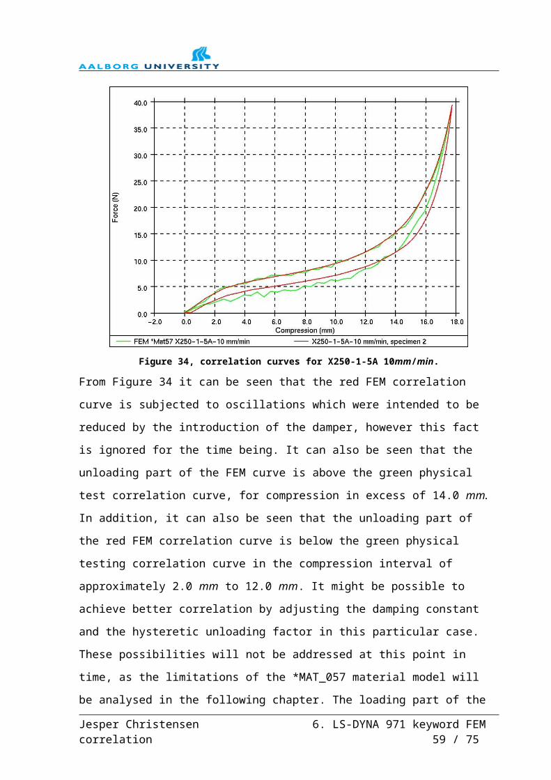
The resulting force vs. displacement curve for model number 1 and the corresponding curve

extracted from the MIRA test data can be seen in Figure 53 below.

Figure 53, correlation curves for model number 1.

The corresponding curves for model number 2, i.e. the square specimen can be seen in Figure

54.

Figure 54, correlation curves for model number 2.

Jesper Christensen Appendix E xi

By comparing Figure 53 to Figure 54 it can be seen that the overall shape of the loading

graphs are similar. In Figure 53 the force increase from 5.0 mm to 20.0 mm compression is

approximately 4 N. The peak force value is approximately 62.4 N. This means that

approximately 6% of the total force increase is spread across the engineering strain value

interval from 0.1 to 0.4. Correspondingly approximately 8% of the total force increase for

model number 2 occurs in the same engineering strain interval, i.e. in the interval from

approximately 10 mm to 40 mm compression.

In addition in excess of 50 % of the total force increase occurs in the interval from 0.7 to 0.8

engineering strain for both models. Furthermore the values of the hysteretic unloading factors

and the shape factors, as listed in Table 15, are very similar, however these are based upon

visual assessments. Finally the engineering strain vs. the engineering strain graphs for the two

FEM models are plotted in Figure 55, which also appear to be very similar.

Figure 55, engineering strain vs. engineering stress.

The difference in peak engineering stress values between the two models is approximately

13%, where the difference in the engineering strain value for which the maximum engineering

stress values are found is 0.01. The difference in energy dissipation between the two models is

very low, approximately 1 %.

These differences could be explained by shape effects. However, during the correlation

process documented by the main report a difference of peak force values up to 50% was

allowed before taking multiple specimens into account in relation to the correlation process.

Jesper Christensen Appendix E xii

Therefore the above differences could also be caused by varying material characteristics

throughout the original foam block, i.e. the block from which the above specimens were cut.

The above results indicate that the influence of shape effects on the FEM correlation process

is low, at least in this particular case. However, as previously stated the above results only

represent the 10 mm/min test for two specimens cut out of the same block of foam. Therefore

it is necessary to analyse the results obtained by similar tests conducted at identical and at

other test speeds before making a general statement. Unfortunately this has, as previously

stated, not been possible due to corrupted test data.

However, the test data of two other cylindrical and two other square specimens at a test speed

of 10 mm/min are available. Therefore, the focus is now aimed upon comparing the MIRA

test results from these tests, in an attempt to better assess whether the above differences are

due to rate effects or varying material characteristics throughout the original foam block.

Subsequently the following discussions will not be based upon results from Finite Element

Analysis.

Influence of shape effects – physical testing

A total of 6 specimens used in this appendix have been cut from the same block of foam, the

specimens are listed in Table 16 below.Table 16, specimen dimensions.

Specimen number

Specimen geometry

Diameter(mm)

Width / depth (mm)

Height (mm)

Maximum displacement value (mm)

C1 Cylindrical 50 50 40C2 Cylindrical 50 50 40C3 Cylindrical 50 49 40S1 Square 100 100 80S2 Square 100 100 80S3 Square 100 100 80

The specimens used for the previously conducted FEM analysis are C3 and S3 respectively.

As Table 16 reveals, these related specimens are very similar in dimensions, in fact the only

“abnormality” is the height of the C3 specimen which is 49 mm as opposed to 50 mm for the

other two cylindrical specimens. The force vs. compression graphs for the three cylindrical

specimens can be seen in Figure 56.

Jesper Christensen Appendix E xiii

Figure 56, force vs. compression MIRA test results, cylindrical specimens.

Figure 56 shows that the curves for specimen 1 and 2 are, to the naked eye coinciding. The

loading part of the curve for specimen 3, which was the specimen used in the above

correlation process, deviates slightly from the two others, but the peak force value is almost

identical for the three specimens. The unloading curves for all three specimens are coinciding.

Figure 57 displays the equivalent curves for the square specimens.

Figure 57, force vs. compression MIRA test results, square specimens.

Jesper Christensen Appendix E xiv

Figure 57 reveals that analogue to the cylindrical specimen number 3 is the odd one out. In

addition the curves for specimen 1 and 2 are near coinciding. Specimen number 3 does not

seem to “stiffen up” in the interval below 10 mm compression, as is the case of specimen 1

and 2. On the other hand specimen 3 seems to “stiffen up” even more so than specimen 1 and

2 in the interval above 70 mm compression. The difference in peak force value of specimen 3

and specimen 1 / 2 is approximately 14 %, which when compared to the differences found

during the correlation process of the main report, is small.

The results of the MIRA testing, as illustrated by Figure 56 and Figure 57 therefore suggests

that in this case the material characteristics do not seem to change significantly from

specimen to specimen. This substantiates the theory that the differences found during the

FEM correlation process in this report is mainly due to shape effects not because of varying

material characteristics throughout the original foam block.

Jesper Christensen Appendix E xv

Documents

Introduction - Aalborg Universitetprojekter.aau.dk/projekter/files/17606498/CAE... · Web viewAnother LS-DYNA material model, *MAT _083, is sometimes also used in these types of analyses