Neutrinos: Fast & Curious

Gabriela BarenboimDepartament de Física Teòrica and IFIC, Universitat de València- CSICCarrer Dr. Moliner 50, E-46100 Burjassot (València), Spain

AbstractThe Standard Model has been effective way beyond expectations in foreseeingthe result of almost all the experimental tests done up so far. In it, neutrinosare massless. Nonetheless, in recent years we have collected solid proofs indi-cating little but non zero masses for the neutrinos (when contrasted with thoseof the charged leptons). These masses permit neutrinos to change their flavorand oscillate, indeed a unique treat. In these lectures, I discuss the propertiesand the amazing potential of neutrinos in and beyond the Standard Model.

1 IntroductionLast decade witnessed a brutal transformation in neutrino physics. It has been experimentally observedthat neutrinos have nonzero masses, implying that leptons blend. This fact was demonstrated by theexperimental evidence that neutrinos can change from one state, or “flavour”, to another. All the in-formation we have accumulated about neutrinos, is quite recent. Less that twenty years old. Neutrinophysics as a solid science is in its teenage years and therefore as any adolescence, in a wild and veryexciting (and excited) state.

However, before jumping into the late "news" about neutrinos, lets understand how and why neu-trinos were conceived.

The ’20s saw the death of numerous sacred cows, and physics was no exemption. One of physic’smost holly principles, energy conservation, apparently showed up not to hold inside the subatomic world.

For some radioactive nuclei, it appeared that a non-negligible fraction of its energy simply van-ished, leaving no trace of its presence.

In 1920, in a (by now famous) letter to a meeting [1], Pauli quasi apologetically wrote,"Dearradioactive Ladies and Gentlemen, ... as a desperate remedy to save the principle of energy conservationin beta decay, ... I propose the idea of a neutral particle of spin half". Pauli hypothesised that themissing energy was taken off by another particle, whose properties were such that made it invisible andimpossible to detect: it had no electric charge, no mass and only very rarely interacted with matter. Alongthese lines, the neutrino was naturally introduced to the universe of particle physics.

Before long, Fermi postulated the four-Fermi Hamiltonian in order to describe beta decay utilisingthe neutrino, electron, neutron and proton. Another field was born: weak interactions took the stage tonever leave it.

Closing the loop, twenty years after Pauli’s letter, Cowan and Reines got the experimental signa-ture of anti-neutrinos emitted by a nuclear power plant.

As more particles who participated in weak interactions were found in the years following neutrinodiscovery, weak interactions got credibility as an authentic new force of nature and the neutrino got to bea key element of it.

Further experimental tests through the span of the following 30 years demonstrated that there werenot one but three sort, or “flavours” of neutrinos (electron neutrinos (νe), muon neutrinos (νµ) and tauneutrinos (ντ )) and that, to the extent we could test, had no mass (and no charge) whatsoever.

The neutrino adventure could have easily finish there, however new analyses in neutrinos comingfrom the sun shown us that the neutrino saga was just beginning....

arX

iv:1

610.

0983

5v1

[he

p-ph

] 3

1 O

ct 2

016

In the canonical Standard Model, neutrinos are completely massless and as a consequence areflavour eigenstates,

W+ −→ e+ + νe ; Z −→ νe + ν̄e

W+ −→ µ+ + νµ ; Z −→ νµ + ν̄µ (1)

W+ −→ τ+ + ντ ; Z −→ ντ + ν̄τ

Precisely because they are massless, they travel at the speed of light and accordingly their flavour doesnot change from generation up to detection. It is evident then, that as flavour is concerned, zero massneutrinos are not an attractive object to study, specially when contrasted with quarks.

However, if neutrinos were massive, and these masses where not degenerate (degenerate massesflavour-wise is identical to the zero mass case) would mean that neutrino mass eigenstates exist νi, i =1, 2, . . ., each with a massmi. The impact of leptonic mixing becomes apparent by looking at the leptonicdecays, W+ −→ νi + `α of the charged vector boson W . Where, α = e, µ, or τ , and `e refers to theelectron, `µ the muon, or `τ the tau.

We call particle `α as the charged lepton of flavour α. Mixing basically implies that when thecharged boson W+ decays to a given kind of charged lepton `α, the neutrino that goes along is notgenerally the same mass eigenstate νi. Any of the different νi can appear.

The amplitude for the decay of a vector boson W+ to a particular mix `α + νi is given by U∗αi.

The neutrino that is radiated in this decay alongside the given charged lepton `α is then

|να >=∑i

U∗αi |νi > . (2)

This specific mixture of mass eigenstates yields the neutrino of flavour α.

The different Uαi can be gathered in a unitary matrix (in the same way they were collected in theCKM matrix in the quark sector) that receives the name of the leptonic mixing matrix orUPNMS [2]. Theunitarity of U ensures that each time a neutrino of flavour α through its interaction produces a chargedlepton, the produced charged lepton will always be `α, the charged lepton of flavour α. That is, a νeproduces exclusively an e, a νµ exclusively a µ, and in a similar way ντ a τ .

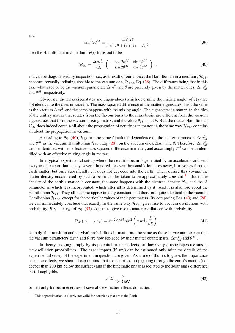
The expression (2), portraying each neutrino of a given flavour as a linear combination of thethree mass eigenstates, can be easily inverted to depict every mass eigenstate νi as an analogous linearcombination of the three flavours:

|νi >=∑α

Uαi |να > . (3)

The amount of α-flavour (or the α-fraction) of νi is obviously |Uαi|2. When a νi interacts and creates acharged lepton, this α-content (or fraction) expresses the probability that the created charged lepton beof flavour α.

2 Neutrino Oscillations basicsThe phenomenon of neutrino morphing, flavour transition or in short oscillation, can be understood inthe following form.

A neutrino is created or emitted by a source along with a charged lepton `α of flavour α. In thisway, at the emission point, the neutrino does have a definite flavour. It is a να. After that point, afterproduction, the neutrino covers some length (propagates thorough a distance) L until it is absorbed.

At this point, when it has already covered the distance to the target, the neutrino interacts and theseinteractions create another charged lepton `β of flavour β, which we can detect. In this way, at the target,

2

we can know that the neutrino is again a neutrino of definite flavour, a νβ . Of course there is a chancethat β 6= α (for instance, if `α is a µ however `β is a τ ), then, all along his journey from the source to theidentification point, the neutrino has morphed or transformed from a να into a νβ .

This transition from one flavour to the other, να −→ νβ , is a canonical case of the widely knownquantum-mechanical effect present in a variety of two state systems and not a particular property ofneutrinos.

Since, as shown clearly by Eq. (2), a να is truly a coherent superposition of the three mass eigen-states νi, the neutrino that travels since it is born until it is detected, can be any of the three νi’s. Becauseof that, we should include the contributions of each of the νi in a coherent way. As a consequence, thetransition amplitude, Amp(να −→ νβ) receives a contribution of each νi and turns out to be the productof three pieces. The first factor is the amplitude for the neutrino created at the generation point alongwith a charged lepton `α to be, particularly, a νi. And as we have said already, it is given by U∗

αi.

The second component of our product is the amplitude for the νi made by the source to cover thedistance up to the detector . We will name this element Prop(νi) for the time being and will postpone thecalculation of its value until later. The last (third) piece is the amplitude for the charged lepton born outof the interaction of the neutrino νi with the target to be, particularly, a `β .

Being the Hamiltonian that describes the interactions between neutrinos, charged leptons andcharged bosons W bosons hermitian (otherwise probability won’t be conserved), it follows that ifAmp(W −→ `ανi) = U∗

αi, then Amp (νi −→ `βW ) = Uβi. In this way, the third and last compo-nent of the product the νi contribution is given by Uβi, and

Amp(να −→ νβ) =∑i

U∗αi Prop(νi) Uβi . (4)

Fig. 1: Neutrino flavour change (oscillation) in vacuum

It still remains to be established the value of Prop(νi). To determine it, we’d better study the νi inits rest frame. We will label the time in that system τi. If νi does have a rest mass mi, then in this frameof reference its state vector satisfies the good old Schrödinger equation

i∂

∂τi|νi(τi) > = mi|νi(τi) > . (5)

whose solution is given clearly by

|νi(τi) > = e−imiτi |νi(0) > . (6)

Then, the amplitude for a given mass eigenstate νi to travel freely during a time τi, is simply the amplitude< νi(0)|νi(τi) > for observing the initial state νi, |νi(0) > after some time as the evoluted state |νi(τi) >,

3

ie. exp[−imiτi]. Thus Prop(νi) is only this amplitude where we have used that the time taken by νi tocover the distance from the source to the detector is just τi, the proper time.

Nevertheless, if we want Prop(νi) to be of any use to us, we must write it first in terms of variableswe can measure, this means to express it, in variables in the lab frame. The natural choice is obviouslythe distance, L, that the neutrino covers between the source and the detector as seen in the lab frame,and the time, t, that slips away during the journey, again in the lab frame. The distance L is set by theexperimentalists through the selection of the place of settlement of the source and that of the detectorand is unique to each experimental setting. Likewise, the value of t is selected by the experimentaliststhrough their election for the time at which the neutrino is made and that when it dies (or gets detected).Therefore, L and t are determined (hopefully carefully enough) by the experiment design, and are thesame for all the νi in the beam. The different νi do travel through an identical distance L, in an identicaltime t.

We still have two additional lab frame variables to determine, the energy Ei and three momentumpi of the neutrino mass eigenstate νi. By using the Lorentz invariance of the four component inter-nal product (scalar product), we can obtain the expression for the miτi appearing in the νi propagatorProp(νi) in terms of the (easy to measure) lab frame variable we have been looking for, which is givenby

miτi = Eit− piL . (7)

At this point however one may argue that, in real life, neutrino sources are basically constant intime, and that the time t that slips away since the neutrino is produced till it dies in the detector is actuallynot measured. This argument is absolutely right. In reality, an experiment smears over the time t usedby the neutrino to complete its route. However, lets consider that two constituents of the neutrino beam,the first one with energy E1 and the second one with energy E2 (both measured in the lab frame), addup coherently to the neutrino signal produced in the detector. Now, let us call t to the the time used bythe neutrino to cover the distance separating the production and detection points. Then by the time theconstituent whose energy is Ej (j = 1, 2) arrives to the detector, it has raised a phase factor exp[−iEjt].Therefore, we will have an interference between the E1 and E2 beam participants that will include aphase factor exp[−i(E1 − E2)t]. When smeared over the non-observed travel time t, this factor goesaway, except when E2 = E1. Therefore, only those constituents of the neutrino beam that share the sameenergy contribute coherently to the neutrino oscillation signal [3,4]. Specifically, only the different masseigenstates constituents of the beams that have the same energy weight in. The rest gets averaged out.

Courtesy to is dispersion relation, a mass eigenstate νi, with mass mi, and energy E, has a threemomentum pi whose absolute value is given by

pi =√E2 −m2

i∼= E − m2

i

2E. (8)

Where, we have utilised that as the masses of the neutrinos are miserably small, m2i � E2 for a typical

energy E attainable at any experiment (the lowest energy neutrinos have MeV energies and sub-eVmasses). From Eqs. (7) and (8), it is easy to see that at a given energy E the phase miτi appearing inProp(νi) takes the value

miτi ∼= E(t− L) +m2i

2EL . (9)

As the phase E(t − L) appears in all the interfering terms it will eventually disappear when calculatingthe transition amplitude. After all is a common phase factor (its absolute value is one). Thus, we can getrid of it already now and use

Prop(νi) = exp[−im2i

L

2E] . (10)

4

Plugging this into Eq. (4), we can obtain that the amplitude for a neutrino born as a να to bedetected as a νβ after covering a distance L with energy E yields

Amp(να −→ νβ) =∑i

U∗αi e

−im2i

L2EUβi . (11)

The expression above is valid for an arbitrary number of neutrino flavours and an identical number ofmass eigenstates, as far as they travel through vacuum. The probability P(να −→ νβ) for να −→ νβ canbe found by squaring it, giving

P(να −→ νβ) = |Amp(να −→ νβ)|2

= δαβ − 4∑i>j

<(U∗αiUβiUαjU

∗βj) sin2

(∆m2

ij

L

4E

)

+2∑i>j

=(U∗αiUβiUαjU

∗βj) sin

(∆m2

ij

L

2E

), (12)

with∆m2

ij ≡ m2i −m2

j . (13)

In order to get Eq. (12) we have used that the mixing matrix U is unitary.

The oscillation probability P(να −→ νβ) we have just obtained corresponds to that of a neutrino,and not to an antineutrino, as we have used that the oscillating neutrino was produced along with acharged antilepton ¯̀, and gives birth to a charged lepton ` once it reaches the detector. The correspondingprobability P(να −→ νβ) for an antineutrino oscillation can be obtained from P(να −→ νβ) takingadvantage of the fact that the two transitions να −→ νβ and νβ −→ να are CPT conjugated processes.Thus, assuming that neutrino interactions respect CPT [5],

P(να −→ νβ) = P(νβ −→ να) . (14)

Then, from Eq. (12) we obtain that

P(νβ −→ να; U) = P(να −→ νβ; U∗) . (15)

Therefore, if CPT is a good symmetry (as far as neutrino interactions are concerned), Eq. (12) tells usthat

P( ( )να −→ ( )νβ) = δαβ − 4∑i>j

<(U∗αiUβiUαjU

∗βj) sin2

(∆m2

ij

L

4E

)

+(−) 2∑i>j

=(U∗αiUβiUαjU

∗βj) sin

(∆m2

ij

L

2E

). (16)

These expressions make it clear that if the mixing matrix U is complex, P(να −→ νβ) and P(να −→ νβ)will not be identical, in general. As να −→ νβ and να −→ νβ are CP conjugated processes, P(να −→νβ) 6= P(να −→ νβ) would provide evidence of CP violation in neutrino oscillations (if Nature haschosen its mixing parameters so that the mixing matrix is indeed complex). Until now, CP violation hasbeen observed only in the quark sector, so its measurement in neutrino physics would be quite exciting.

So far, we have been working in natural units. A fact that becomes transparent by looking at thedispersion relation Eq. (9). If we restore now the ~’s and c factors (we have happily set to one) into theoscillation probability we find that

sin2

(∆m2

ij

L

4E

)−→ sin2

(∆m2

ijc4 L

4~cE

)(17)

5

Having done that, it is easy and instructive to explore the semi-classical limit, ~ −→ 0. In this limit theoscillation length goes to zero (the oscillation phase goes to infinity) and the oscillations are averagedto 1/2. The interference pattern is lost. A similar situation appears if we let the mass difference ∆m2

become large. This is exactly what happens in the quark sector (and the reason why we never study quarkoscillations despite knowing that mass eigenstates do not coincide with flavour eigenstates).

In terms of real life units (which are not "natural" units), the oscillation phase is given by

∆m2ij

L

4E= 1.27 ∆m2

ij(eV2)L (km)

E (GeV). (18)

then, since sin2[1.27 ∆m2ij(eV2)L (km)/E (GeV)] can be experimentally observed (ie. not smeared

out) only if its argument is in a ballpark around one, an experimental set-up with a baseline L(km) and an energy E (GeV) is sensitive to neutrino mass squared differences ∆m2

ij(eV2) of order∼ [L (km)/E (GeV]−1. For example, an experiment with a baseline of L ∼ 104 km, roughly the sizeof Earth’s diameter, and E ∼ 1 GeV would explore mass differences ∆m2

ij down to ∼ 10−4 eV2. Thisfact makes it clear that neutrino long-baseline experiments can test even miserably small neutrino massdifferences. It does so by exploiting the quantum mechanical interference between amplitudes whose rel-ative phases are given precisely by these super tiny neutrino mass differences, which can be transformedinto sizeable effects by choosing L/E appropriately.

But let’s keep analysing the oscillation probability and see whether we can learn more aboutneutrino oscillations by studying its expression.

It is clear from P( ( )να −→ ( )νβ) that if neutrinos have zero mass, in such a way that all ∆m2ij = 0,

then, P( ( )να −→ ( )νβ) = δαβ . Therefore, the experimental observation that neutrinos can morph from oneflavour to a different one indicates that neutrinos are not only massive but also that their masses are notdegenerate. Actually, it was precisely this evidence the one that proved beyond any reasonable doubt thatneutrinos are massive.

However, every neutrino oscillation seen so far has involved at some point neutrinos that travelthrough matter. But the expression we derived is valid only for flavour change in vacuum, and does nottake into account any interaction between the neutrinos and the matter traversed between their sourceand their detector. Thus, the question remains whether it may be that some unknown flavour changinginteractions between neutrinos and matter are indeed responsible of the observed flavour transitions, andnot neutrino masses. Regarding this question, a couple of things should be said. First, although it is truethat the Standard Model of elementary particle physics contains only massless neutrinos, it provides anamazingly well corroborated description of weak interactions, and therefore of all the ways a neutrinointeracts. Such a description does not include flavour change. Second, for some of the processes experi-mentally observed where neutrinos do change flavour, matter effects are expected to be miserably small,and on those cases the evidence points towards a dependence on L and E in the flavour transition prob-ability through the combination L/E, as anticipated by the oscillation hypothesis. Modulo a constant,L/E is precisely the proper time that goes by in the rest frame of the neutrino as it covers a distance Lpossessing an energy E. Therefore, these flavour transitions behave as if they were a true progression ofthe neutrino itself over time, and not a result of an interaction with matter.

Now, lets explore the case where the leptonic mixing were trivial. This would imply that in thecharged boson decay W+ −→ `α + νi, which as we established has an amplitude U∗

αi, the emergingcharged antilepton `α of flavour α comes along always with the same neutrino mass eigenstate νi. Thatis, if U∗

αi 6= 0, then due to unitarity, Uαj becomes zero for all j 6= i. Therefore, from Eq. (16) it is clearthat, P( ( )να −→ ( )νβ) = δαβ . Thus, the observation that neutrinos morph indicates non trivial a mixingmatrix.

Then, we are left with basically two ways to detect neutrino flavour change. The first one is toobserve, in a beam of neutrinos which are all created with the same flavour, say α, some amount ofneutrinos of a new flavour β that is different from the flavour α we started with. This goes under the

6

name of appearance experiments. The second way is to start with a beam of identical ναs, whose fluxis either measured or known, and observe that after travelling some distance this flux is depleted. Suchexperiments are called disappearance experiments.

As Eq. (16) shows, the transition probability in vacuum does not only depend on L/E but alsooscillates with it. It is because of this fact that neutrino flavour transitions are named “neutrino oscilla-tions”. Now notice also that neutrino transition probabilities do not depend on the individual neutrinomasses (or masses squared) but on the squared-mass differences. Thus, oscillation experiments can onlymeasure the neutrino mass squared spectrum. Not its absolute scale. Experiments can test the pattern butcannot determine the distance above zero the whole spectra lies.

It is clear that neutrino transitions cannot modify the total flux in a neutrino beam, but simply alterits distribution between the different flavours. Actually, from Eq. (16) and the unitarity of the U matrix,it is obvious that ∑

β

P( ( )να −→ ( )νβ) = 1 , (19)

where the sum runs over all flavours β, including the original one α. Eq. (19) makes it transparent thatthe probability that a neutrino morphs its flavour, added to the probability that it keeps the flavour it hadat birth, is one. Ergo, flavour transitions do not modify the total flux. Nevertheless, some of the flavoursβ 6= α into which a neutrino can oscillate into may be sterile flavours; that is, flavours that do not takepart in weak interactions and therefore escape detection. If any of the original (active) neutrino flux turnsinto sterile, then an experiment able to measure the total active neutrino flux—that is, the flux associatedto those neutrinos that couple to the weak gauge bosons: νe, νµ, and ντ— will observe it to be notexactly the original one, but smaller than it. In the experiments performed up today, no flux was evermissed.

In the literature, description of neutrino oscillations normally assume that the different mass eigen-states νi that contribute coherently to a beam share the same momentum, rather than the same energy aswe have argued they must have. While the supposition of equal momentum is technically wrong, it is aninoffensive mistake, since, as can easily be shown, it conveys to the same oscillation probabilities as theones we have obtained.

A relevant and interesting case of the (not that simple) formula for P(να −→ νβ) is the case whereonly two flavours participate in the oscillation. The only-two-neutrino scenario is a rather rigorousdescription of a vast number of experiments. In fact only recently (and in few experiments) a moresophisticated (three neutrino description) was needed to fit observations. Lets assume then, that only twomass eigenstates, which we will name ν1 and ν2, and two reciprocal flavour states, which we will nameνµ and ντ , are relevant, in such a way that only one squared-mass difference, m2

2 −m21 ≡ ∆m2 arises.

Even more, neglecting phase factors that can be proven to have no impact on oscillation probabilities,the mixing matrix U can be written as(

νµντ

)=

(cos θ sin θ− sin θ cos θ

)(ν1ν2

)(20)

The unitary mixing matrix U of Eq. (20) is just a 2×2 rotation matrix, and as such , parameterized bya single rotation angle θ which is named (in neutrino physics) as the mixing angle. Plugging the Uof Eq. (20) and the unique ∆m2 into the general formula of the transition probability P(να −→ νβ),Eq. (16), we can readily see that, for β 6= α, when only two neutrinos are relevant,

P(να −→ νβ) = sin2 2θ sin2

(∆m2 L

4E

). (21)

Moreover, the survival probability, ie. the probability that the neutrino remains with the same flavour itswas created with is, as expected, one minus the probability that it changes flavour.

7

3 Neutrino Oscillations in a mediumWhen we create a beam of neutrinos on earth through an accelerator and send it up to thousand kilome-tres away to a meet detector, the beam does not move through vacuum, but through matter, earth matter.The beam of neutrinos then scatters from the particles it meets along the way. Such a coherent forwardscattering can have a large effect on the transition probabilities. We will assume for the time being thatneutrino interactions with matter are flavour conserving, as described by the Standard Model, and com-ment on the possibility of flavour changing interactions later. Then as there are only two types of weakinteractions (mediated by charged and neutral currents) the would be accordingly only two possibilitiesfor this coherent forward scattering from matter particles to take place. Charged current mediated weakinteractions will occur only if and only if the incoming neutrino is an electron neutrino. As only the νecan exchange charged boson W with an Earth electron. Thus neutrino-electron coherent forward scatter-ing via W exchange opens up an extra source of interaction energy VW suffered exclusively by electronneutrinos. Obviously, this additional energy being from weak interactions origin has to be proportionalto GF , the Fermi coupling constant. In addition, the interaction energy coming from νe − e scatteringgrows with the number of targets, Ne, the number of electrons per unit volume (given by the density ofthe Earth). Putting everything together it is not difficult to see that

VW = +√

2GF Ne , (22)

clearly, this interaction energy affects also antineutrinos (in a opposite way though). It changes sign ifwe switch the νe by νe.

The interactions mediated by neutral currents correspond to the case where a neutrino in matterinteracts with a matter electron, proton, or neutron by exchanging a neutral Z boson. According to theStandard Model weak interactions are flavour blind. Every flavour of neutrino enjoys them, and theamplitude for this Z exchange is always the same. It also teaches us that, at zero momentum transfer,electrons and protons couple to the Z boson with equal strength. The interaction has though, oppositesign. Therefore, counting on the fact that the matter through which our neutrino moves is electricallyneutral (it contains equal number of electrons and protons), the contribution of both, electrons and protonsto coherent forward neutrino scattering through Z exchange will add up to zero. Consequently onlyinteractions with neutrons will survive so that, the effect of the Z exchange contribution to the interactionpotential energy VZ reduces exclusively to that with neutrons and will be proportional toNn, the numberdensity of neutrons. It goes without saying that it will be equal to all flavours. This time, we find that

VZ = −√

2

2GF Nn , (23)

as was the case before, for VW , this contribution will flip sign if we replace the neutrinos by anti-neutrinos.

But if, as we said, the Standard Model interactions do not change neutrino flavour, neutrino flavourtransitions or neutrino oscillations point undoubtedly to neutrino mass and mixing even when neutrinosare propagating through matter. Unless non-Standard-Model flavour changing interactions play a role.

Neutrino propagation in matter is easy to understand when analysed through the time dependentSchrödinger equation in the lab frame

i∂

∂t|ν(t) > = H|ν(t) > . (24)

where, |ν(t)> is a (three component) neutrino vector state, in which each neutrino flavour correspondsto one component. In the same way, the Hamiltonian H is a (tree × three) matrix in flavour space. Tomake our lives easy, lets analyse the case where only two neutrino flavours are relevant, say νe and νµ.Then

|ν(t) > =

(fe(t)fµ(t)

), (25)

8

with fi(t)2 the amplitude of the neutrino to be a νi at time t. This time the Hamiltonian, H, is a 2×2matrix in neutrino flavour space, i.e., νe − νµ space.

It will prove to be clarifying to work out the two flavour case in vacuum first, and add mattereffects afterwards. Using Eq. (2) to express |να > as a linear combination of mass eigenstates, we cansee that the να − νβ matrix element of the Hamiltonian in vacuum,HVac, can be written as

< να|HVac|νβ > = <∑i

U∗αiνi|HVac|

∑j

U∗βjνj >

=∑j

UαjU∗βj

√p2 +m2

j . (26)

where we are supposing that the neutrinos belong to a beam where all its mass components (the masseigenstates) share the same definite momentum p. As we have already mentioned, despite this suppo-sition being technically wrong, it leads anyway to the right transition amplitude. In the second line ofEq. (26), we have used that the neutrinos νj with momentum p, the mass eigenstates, are the asymptoticstates of the hamiltonian,HVac for which constitute an orthonormal basis, satisfy

HVac|νj >= Ej |νj > (27)

and have the standard dispersion relation, Ej =√p2 +m2

j .

As we have already mentioned, neutrino oscillations are the archetype quantum interference phe-nomenon, where only the relative phases of the interfering states play a role. Therefore, only the relativeenergies of these states, which set their relative phases, are relevant. As a consequence, if it proves tobe convenient (and it will), we can feel free to happily remove from the HamiltonianH any contributionproportional to the identity matrix I . As we have said, this subtraction will leave unaffected the differ-ences between the eigenvalues of H, and therefore will leave unaffected the prediction of H for flavourtransitions.

It goes without saying that as in this case only two neutrinos are relevant, there are only two masseigenstates, ν1 and ν2, and only one mass splitting ∆m2 ≡ m2

2 − m21, and therefore there should be,

as before a unitary U matrix given by Eq. (20) which rotates from one basis to the other. Inserting itinto Eq. (26), and assuming that our neutrinos have low masses as compared to their momenta, i.e.,(p2 + m2

j )1/2 ∼= p + m2

j/2p, and removing from HVac a term proportional to the the identity matrix (aremoval we know is going to be harmless), we get

HVac =∆m2

4E

(− cos 2θ sin 2θ

sin 2θ cos 2θ

). (28)

To write this expression, the highly relativistic approximation, which says that p ∼= E is used. Where Eis the average energy of the neutrino mass eigenstates in our neutrino beam of ultra high momentum p.

It is not difficult to corroborate that the HamiltonianHVac of Eq. (28) for the two neutrino scenariowould give an identical oscillation probability , Eq. (21), as the one we have already obtained in adifferent way. An easy way to do it is to analyse the transition probability for the process νe −→ νµ.From Eq. (20) it is clear that in terms of the mixing angle, the electron neutrino state composition is

|νe > = |ν1 > cos θ + |ν2 > sin θ , (29)

while that of the muon neutrino is given by

|νµ > = −|ν1 > sin θ + |ν2 > cos θ . (30)

In the same way, we can also write the eigenvalues of the vacuum hamiltonian HVac, Eq.25, in terms ofthe mass squared differences as

λ1 = −∆m2

4E, λ2 = +

∆m2

4E. (31)

9

The mass eigenbasis of this Hamiltonian, |ν1 > and |ν2 >, can also be written in terms of flavoureigenbasis |νe > and |νµ > by means of Eqs. (29) and (30). Therefore, the Schrödinger equation ofEq. (24), with the identification ofH in this case withHVac tells us that if at time t = 0 we begin from a|νe >, then once some time t elapses this |νe > will progress into the state given by

|ν(t) > = |ν1 > e+i∆m2

4Et cos θ + |ν2 > e−i

∆m2

4Et sin θ . (32)

Thus, the probability P(νe −→ νµ) that this evoluted neutrino be detected as a different flavour νµ, fromEqs. (30) and (32), is given by,

P(νe −→ νµ) = | < νµ|ν(t) > |2

= | sin θ cos θ(−ei∆m2

4Et + e−i

∆m2

4Et)|2

= sin2 2θ sin2

(∆m2 L

4E

). (33)

Where we have substituted the time t travelled by our highly relativistic state by the distance L it hascovered. The flavour transition or oscillation probability of Eq. (33), as expected, is exactly the same wehave found before, Eq. (21).

We can now move on to analyse neutrino propagation in matter. In this case, the 2×2 Hamiltonianrepresenting the propagation in vacuumHVac receives the two additional contributions we have discussedbefore, and becomesHM , which is given by

HM = HVac + VW

(1 00 0

)+ VZ

(1 00 1

). (34)

In the new Hamiltonian, the first additional contribution corresponds to the interaction potential due to thecharged bosons exchange, Eq. (22). As this interaction is suffered only by νe, this contribution is differentfrom zero only in the HM (1,1) element or the νe − νe element. The second additional contribution, thelast term of Eq. (34) comes from the Z boson exchange, Eq. (23). Since this interaction is flavour blind,it affects every neutrino flavour in the same way, its contribution to HM is proportional to the identitymatrix, and can be safely neglected. Thus

HM = HVac +VW2

+VW2

(1 00 −1

), (35)

where (for reasons that are going to become clear later) we have divided the W -exchange contributioninto two pieces, one proportional to the identity (that we will disregarded in the next step) and, a piecethat it is not proportional to the identity, that we will keep. Disregarding the first piece as promised, wehave from Eqs. (28) and (35)

HM =∆m2

4E

(−(cos 2θ −A) sin 2θ

sin 2θ (cos 2θ −A)

), (36)

where we have defined

A ≡ VW /2

∆m2/4E=

2√

2GFNeE

∆m2. (37)

Clearly, A parameterizes the relative size of the matter effects as compared to the vacuum contributiongiven by the neutrino squared-mass splitting and signals the situations when they become important.

Now, if we introduce (a physically meaningful) short-hand notation

∆m2M ≡ ∆m2

√sin2 2θ + (cos 2θ −A)2 (38)

10

and

sin2 2θM ≡ sin2 2θ

sin2 2θ + (cos 2θ −A)2, (39)

then the Hamiltonian in a mediumHM turns out to be

HM =∆m2

M

4E

(− cos 2θM sin 2θM

sin 2θM cos 2θM

). (40)

and can be diagonalised by inspection, i.e., as a result of our choice, the Hamiltonian in a medium ,HM ,becomes formally indistinguishable to the vacuum one,HVac, Eq. (28). The difference being that in thiscase what used to be the vacuum parameters ∆m2 and θ are presently given by the matter ones, ∆m2

M

and θM , respectively.

Obviously, the mass eigenstates and eigenvalues (which determine the mixing angle) of HM arenot identical to the ones in vacuum. The mass squared difference of the matter eigenstates is not the sameas the vacuum ∆m2, and the same happens with the mixing angle. The eigenstates in matter, ie. the filesof the unitary matrix that rotates from the flavour basis to the mass basis, are different from the vacuumeigenvalues that form the vacuum mixing matrix, and therefore θM is not θ. But, the matter HamiltonianHM does indeed contain all about the propagation of neutrinos in matter, in the same wayHVac containsall about the propagation in vacuum.

According to Eq. (40), HM has the same functional dependence on the matter parameters ∆m2M

and θM as the vacuum HamiltonianHVac, Eq. (28), on the vacuum ones, ∆m2 and θ. Therefore, ∆m2M

can be identified with an effective mass squared difference in matter, and accordingly θM can be uniden-tified with an effective mixing angle in matter.

In a typical experimental set-up where the neutrino beam is generated by an accelerator and sentaway to a detector that is, say, several hundred, or even thousand kilometres away, it traverses throughearth matter, but only superficially , it does not get deep into the earth. Then, during this voyage thematter density encountered by such a beam can be taken to be approximately constant 1. But if thedensity of the earth’s matter is constant, the same happens with the electron density Ne, and the Aparameter in which it is incorporated, which after all is determined by it. And it is also true about theHamiltonian HM . They all become approximately constant, and therefore quite identical to the vacuumHamiltonianHVac, except for the particular values of their parameters. By comparing Eqs. (40) and (28),we can immediately conclude that exactly in the same way HVac gives rise to vacuum oscillations withprobability P(νe −→ νµ) of Eq. (33),HM must give rise to matter oscillations with probability

PM (νe −→ νµ) = sin2 2θM sin2

(∆m2

M

L

4E

). (41)

Namely, the transition and survival probabilities in matter are the same as those in vacuum, except thatthe vacuum parameters ∆m2 and θ are now replaced by their matter counterparts, ∆m2

M and θM .

In theory, judging simply by its potential, matter effects can have very drastic repercussions inthe oscillation probabilities. The exact impact (if any) can be estimated only after the details of theexperimental set-up of the experiment in question are given. As a rule of thumb, to guess the importanceof matter effects, we should keep in mind that for neutrinos propagating through the earth’s mantle (notdeeper than 200 km below the surface) and if the kinematic phase associated to the solar mass differenceis still negligible,

A ∼=E

13 GeV(42)

so that only for beam energies of several GeV matter effects do matter.1This approximation is clearly not valid for neutrinos that cross the Earth

11

And how much do they matter? They matter a lot! From Eq. (39) for the matter mixing angle, θM ,we can appreciate that even when the vacuum mixing angle θ is incredible small, say, sin2 2θ = 10−4,if we get to have A ∼= cos 2θ, i.e., for energies of a few tens of GeV, then sin2 2θM can be brutallyenhanced as compared to its vacuum value and can even reach maximal mixing, ie. sin2 2θM = 1. Thiswild enhancement of a small mixing angle in vacuum up to a sizeable (even maximal) one in matter is the“resonant” enhancement, the largest possible version of the Mikheyev-Smirnov-Wolfenstein effect [6–9].In the beginning of solar neutrino experiments, people entertained the idea that this brutal enhancementwas actually taking place while neutrinos crossed the sun. Nonetheless, as we will see soon the mixingangle associated with solar neutrinos is quite sizeable (∼ 34◦) already in vacuum [10]. Then, althoughmatter effects on the sun are important and they do enhance the solar mixing angle, unfortunately theyare not as drastic as we once dreamt. Nevertheless, for long-baselines they will play (they are alreadyplaying!) a key role in the determination of the ordering of the neutrino spectrum.

4 Evidence for neutrino oscillations4.1 Atmospheric and Accelerator NeutrinosAlmost twenty years have elapsed since we were presented solid and convincing evidence of neutrinomasses and mixings, and since then, the evidence has only grown. SuperKamiokande (SK) was the firstexperiment to present compelling evidence of νµ disappearance in their atmospheric neutrino fluxes,see [11] . In Fig. 2 the zenith angle (the angle subtended with the horizontal) dependence of the multi-GeV νµ sample is shown together with the disappearance as a function of L/E plot. These data fitamazingly well the naive two component neutrino hypothesis with

∆m2atm = 2− 3× 10−3eV2 and sin2 θatm = 0.50± 0.13 (43)

Roughly speaking SK corresponds to an L/E for oscillations of 500 km/GeV and almost maximal mix-ing (the mass eigenstates are nearly even admixtures of muon and tau neutrinos). No signal of an in-volvement of the third flavour, νe is found so the assumption is that atmospheric neutrino disappearanceis basically νµ −→ ντ . Notice however, that the first NOvA results seem to point toward a mixing anglewhich is not maximal (excluding maximal mixing at the 2 sigma level).

Fig. 2: Superkamiokande’s evidence for neutrino oscillations both in the zenith angle and L/E plots

After atmospheric neutrino oscillations were established, a new series of neutrino experimentswere built, sending (man-made) beams of νµ neutrinos to detectors located at large distances: the K2K

12

(T2K) experiment [12,13], sends neutrinos from the KEK accelerator complex to the old SK mine, with abaseline of 120 (235) km while the MINOS (NOvA) experiment [14,15], sends its beam from Fermilab,near Chicago, to the Soudan mine (Ash river) in Minnesota, a baseline of 735 (810) km. All theseexperiments have seen evidence for νµ disappearance consistent with the one found by SK. Their resultsare summarised in Fig. 3.

Fig. 3: Allowed regions in the ∆m2atm vs sin2 θatm plane for MINOS data as well as for T2K data and two of

the SK analyses. MINOS’s best fit point is at sin2 θatm = .51 and ∆m2atm = 2.37 × 10−3eV2. Notice that new

NOvA data seem to exclude maximal mixing at the 2 sigma level

4.2 Reactor and Solar NeutrinosThe KamLAND reactor experiment, an antineutrino disappearance experiment, receiving neutrinos fromsixteen different reactors, at distances ranging from hundred to thousand kilometres, with an averagebaseline of 180 km and neutrinos of a few eV, [16, 17], has seen evidence of neutrino oscillations . Suchevidence was collected not only at a different L/E than the atmospheric and accelerator experiments butalso consists on oscillations involving electron neutrinos, νe, the ones which were not involved before.These oscillations have also been seen for neutrinos coming from the sun (the sun produces only electronneutrinos). However,in order to compare the two experiments we should assume that neutrinos (solar)and antineutrinos (reactor) behave in the same way, ie. assume CPT conservation. The best fit values in

13

the two neutrino scenario for the KamLAND experiment are

∆m2� = 8.0± 0.4× 10−5eV2 and sin2 θ� = 0.31± 0.03 (44)

In this case, the L/E involved is 15 km/MeV which is more than an order of magnitude larger than theatmospheric scale and the mixing angle, although large, is clearly not maximal.

Fig. 4 shows the disappearance probability for the ν̄e for KamLAND as well as several olderreactor experiments with shorter baselines 2.The second panel depicts the flavour content of the 8Boronsolar neutrino flux (with GeV energies) measured by SNO, [18], and SK, [19]. The reactor outcomecan be explained in terms of two flavour oscillations in vacuum, given that the fit to the disappearanceprobability, is appropriately averaged over E and L..

Fig. 4: Disappearance of the ν̄e observed by reactor experiments as a function of distance from the reactor. Theflavour content of the 8Boron solar neutrinos for the various reactions for SNO and SK. CC: νe+d −→ e−+p+p,NC:νx + d −→ νx + p+ n and ES: να + e− −→ να + e−

The analysis of neutrinos originating from the sun is marginally more complex that the one wedid before because it should incorporate the matter effects that the neutrinos endure since they are born(at the centre of the sun) until they abandon it, which are imperative at least for the 8Boron neutrinos.The pp and 7Be neutrinos are less energetic and therefore are not significantly altered by the presenceof matter and leave the sun as though it were ethereal. 8Boron neutrinos on the other hand, leave thesun unequivocally influenced by the presence of matter and this is evidenced by the fact that they leavethe sun as ν2, the second mass eigenstate and therefore do not experience oscillations. This distinctionamong neutrinos coming from different reaction chains is, as mentioned, due mainly to their disparitiesat birth. While pp (7Be) neutrinos are created with an average energy of 0.2 MeV (0.9 MeV), 8B are bornwith 10 MeV and as we have seen the impact of matter effects grows with the energy of the neutrino.

However, we ought to emphasise that we do not really see solar neutrino oscillations. To tracethe oscillation pattern, to be able to test is distinctive shape, we need a kinematic phase of order oneotherwise the oscillations either do not develop or get averaged to 1/2. In the case of neutrinos comingfrom the sun the kinematic phase is

∆� =∆m2

�L

4E= 107±1. (45)

Consequently, solar neutrinos behave as "effectively incoherent" mass eigenstates once they leave thesun, and remain so once they reach the earth. Consequently the νe disappearance or survival probability

2Shorter baseline reactor neutrino experiments, which has seen no evidence of flux depletion suffer the so-called reactorneutrino anomaly, which may point toward the existence of light sterile states

14

is given by

〈Pee〉 = f1 cos2 θ� + f2 sin2 θ� (46)

where f1 is the ν1 content or fraction of νµ and f2 is the ν2 content of νµ and therefore both fractionssatisfy

f1 + f2 = 1. (47)

Nevertheless, as we have already mentioned, solar neutrinos originating from the pp and 7Be chains arenot affected by the solar matter and oscillate as in vacuum and thus, in their case f1 ≈ cos2 θ� = 0.69and f2 ≈ sin2 θ� = 0.31. In the 8B a neutrino case, however, the impact of solar matter is sizeable andthe corresponding fractions are substantially altered, see Fig. 5.

Fig. 5: The sun produces νe in the core but once they exit the sun thinking about them in the mass eigenstate basisis useful. The fraction of ν1 and ν2 is energy dependent above 1 MeV and has a dramatic effect on the 8Boronsolar neutrinos, as first observed by Davis.

In a two neutrino scenario, the day-time CC/NC measured by SNO, which is roughly identical tothe day-time average νe survival probability, 〈Pee〉, reads

CC

NC

∣∣∣∣day

= 〈Pee〉 = f1 cos2 θ� + f2 sin2 θ�, (48)

where f1 and f2 = 1 − f1 are the ν1 and ν2 contents of the muon neutrino, respectively, averaged overthe 8B neutrino energy spectrum appropriately weighted with the charged current current cross section.Therefore, the ν1 fraction (or how much f2 differs from 100% ) is given by

f1 =

(CCNC

∣∣day − sin2 θ�

)cos 2θ�

=(0.347− 0.311)

0.378≈ 10% (49)

where the central values of the last SNO analysis, [18], were used. As there are strong correlationsbetween the uncertainties of the CC/NC ratio and sin2 θ� it is not obvious how to estimate the uncertaintyon f1 from their analysis. Note, that if the fraction of ν2 were 100%, then CC

NC

∣∣day = sin2 θ�.

Utilising the analytic analysis of the Mikheyev-Smirnov-Wolfenstein (MSW) effect, gave in [20],one can obtain the mass eigenstate fractions in a medium, which are given by

f2 = 1− f1 = 〈sin2 θM� + Px cos 2θM� 〉8B, (50)

with θM� being the mixing angle as given at the νe production point and Px is the probability of theneutrino to hop from one mass eigenstate to the second one during the Mikheyev-Smirnov resonance

15

crossing. The average 〈...〉8B is over the electron density of the 8B νe production region in the centreof the Sun as given by the Solar Standard Model and the energy spectrum of 8B neutrinos has beenappropriately weighted with SNO’s charged current cross section. All in all, the 8B energy weightedaverage content of ν2’s measured by SNO is

f2 = 91± 2% at the 95 % C.L.. (51)

Therefore, it is obvious that the 8B solar neutrinos are the purest mass eigenstate neutrino beam knownso far and SK super famous picture of the sun taken (from underground) with neutrinos is made withapproximately 90% of ν2, ie. almost a pure beam of mass eigenstates.

On March 8, 2012 a newly built reactor neutrino experiment, the Daya Bay experiment, located inChina, announced the measurement of the third mixing angle [21], the only one which was still missingand found it to be

sin2(2θ12) = 0.092± 0.017 (52)

Following this announcement, several experiments confirmed the finding and during the last years thelast mixing angle to be measured became the best (most precisely) measured one. The fact that thisangle, although smaller that the other two, is still sizeable opens the door to a new generation of neutrinoexperiments aiming to answer the open questions in the field.

5 ν Standard ModelNow that we have comprehended the physics behind neutrinos oscillations and have leaned the experi-mental evidence about the parameters driving these oscillations, we can move ahead and construct theNeutrino Standard Model:

– it comprises three light (mi < 1 eV) neutrinos, ie. it involves just two mass differences∆m2

atm ≈ 2.5× 10−3eV2 and ∆m2solar ≈ 8.0× 10−5eV2 .

– so far we have not seen any solid experimental indication (or need) for additional neutrinos 3. Aswe have measured long time ago the invisible width of the Z boson and found it to be 3, withinerrors, if additional neutrinos are going to be incorporated into the model, they cannot couple tothe Z boson, ie. they cannot enjoy weak interactions, so we call them sterile. However, as sterileneutrinos have not been seen (although they may have been hinted), and are not needed to explainany solid experimental evidence, our Neutrino Standard Model will contain just the three activeflavours: e, µ and τ .

– the unitary mixing matrix which rotates from the flavour to the mass basis, called the PMNS matrix,comprises three mixing angles (the so called solar mixing angle:θ12, the atmospheric mixing angleθ23, and the last to be measured, the reactor mixing angleθ13) , one Dirac phase (δ) and potentiallytwo Majorana phases (α, β) and is given by

| να〉 = Uαi | νi〉

Uαi =

1c23 s23−s23 c23

c13 s13e−iδ

1−s13eiδ c13

c12 s12−s12 c12

1

1eiα

eiβ

where sij = sin θij and cij = cos θij . Courtesy of the hierarchy in mass differences (and to a lessextent to the smallness of the reactor mixing angle) we are permitted to recognise the (23) label inthe three neutrino scenario as the atmospheric ∆m2

atm we obtained in the two neutrino scenario, in

3Although it must be noted that there are several not significant hint pointing in this direction

16

Fig. 6: Flavour content of the three neutrino mass eigenstates (not including the dependence on the cosine of theCP violating phase δ).If CPT is conserved, the flavour content must be the same for neutrinos and anti-neutrinos.Notice that oscillation experiments cannot tell us how far above zero the entire spectrum lies.

a similar fashion the (12) label can be assimilated to the solar ∆m2�. The (13) sector drives the νe

flavour oscillations at the atmospheric scale, and the depletion in reactor neutrino fluxes see [23].According to the experiments done so far, the three sigma ranges for the neutrino mixing anglesare

0.267 < sin2 θ12 < 0.344 ; 0.342 < sin2 θ23 < 0.667 ; 0.0156 < sin2 θ13 < 0.0299

while the corresponding ones for the mass splittings are

2.24× 10−3eV2 < | ∆m232 | < 2.70× 10−3eV2

and

7.× 10−5eV2 < ∆m221 < 8.09× 10−5eV2.

These mixing angles and mass splittings are summarised in Fig. 6.– As oscillation experiments only explore the two mass differences, two ordering are possible, as

shown in Fig. 6. They are called normal and inverted hierarchy and roughly identify whether themass eigenstate with the smaller electron neutrino content is the lightest or the heaviest.

– The absolute mass scale of the neutrinos, or the mass of the lightest neutrino is not know yet, butcosmological bounds already say that the heaviest one must be lighter than about .5 eV.

– As transition or survival probabilities depend on the combination U∗αiUβi no trace of the Majorana

phases could appear on oscillation phenomena, however they will have observable effects in thoseprocesses where the Majorana character of the neutrino is essential for the process to happen, likeneutrino-less double beta decay.

6 Neutrino mass and character6.1 Absolute Neutrino MassThe absolute mass scale of the neutrino, ie. the mass of the lightest/heaviest neutrino, cannot be obtainedfrom oscillation experiments, however this does not mean we have no access to it. Direct experiments liketritium beta decay, or neutrinoless double beta decay and indirect ones, like cosmological observations,have potential to feed us the information on the absolute scale of neutrino mass, we so desperately need.The Katrin tritium beta decay experiment, [24], has sensitivity down to 200 meV for the "mass" of νedefined as

mνe =| Ue1 |2 m1+ | Ue2 |2 m2+ | Ue3 |2 m3. (53)

17

Fig. 7: The effective mass measured in double β decay, in cosmology and in Tritium β decay versus the mass ofthe lightest neutrino. Below the dashed lines, only the normal hierarchy is allowed. Notice that while double βdecay experiments bound the neutrino mass only in the Majorana case, Planck bounds apply for either case

Neutrino-less double beta decay experiments, see [25] for a review, do not measure the absolutemass of the neutrino directly but a particular combination of neutrino masses and mixings,

mββ =|∑

miU2ei |=| mac

213c

212 +m2c

213s

212e

2iα +m3s213e

2iβ |, (54)

where it is understood that neutrinos are taken to be Majorana particles, ie. truly neutral particles (havingall their quantum numbers to be zero). The new generation of experiments seeks to reach below 10 meVfor mββ in double beta decay.

Cosmological probes (CMB and Large Scale Structure experiments) measure the sum of the neu-trino masses

mcosmo =∑i

mi. (55)

and may have a say on the mass ordering (direct or inverted spectrum) as well as test other neutrinoproperties like neutrino asymmetries [26]. If

∑mi ≈ 10 eV, the energy balance of the universe saturates

the bound coming from its critical density. The current limit, [27], is a few % of this number, ∼ .5

18

eV. These bounds are model dependent but they do all give numbers of the same order of magnitude.However, given the systematic uncertainties characteristic of cosmology, a solid limit of less that 100meV seems way too aggressive.

Fig. 7 shows the allowed parameter space for the neutrino masses (as a function of the absolutescale) for both the normal and inverted hierarchy.

6.2 Majorana vs DiracA fermion mass is nothing but a coupling between a left handed state and a right handed one. Thus, if weexamine a massive fermion at rest, then one can regard this state as a linear combination of two masslessparticles, one right handed and one left handed. If the particle we are examining is electrically charged,like an electron or a muon, both particles, the left handed as well as the right handed must have the samecharge (we want the mass term to be electrically neutral). This is a Dirac mass term. However, for aneutral particle, like a sterile neutrino, a new possibility opens up, the left handed particle can be coupledto the right handed anti-particle, (a term which would have a net charge, if the fields are not absolutelyand totally neutral) this is a Majorana mass term.

Thus a truly and absolutely neutral particle (who will inevitably be its own antiparticle) does havetwo ways of getting a mass term, a la Dirac or a la Majorana, and if there are no reasons to forbid one ofthem, will have them both, as shown in Fig. 6.2.

In the case of a neutrino, the left chiral field couples to SU(2) × U(1) implying that a Majoranamass term is forbidden by gauge symmetry. However, the right chiral field carries no quantum numbers,is totally and absolutely neutral. Then, the Majorana mass term is unprotected by any symmetry and it isexpected to be very large, of the order of the largest scale in the theory. On the other hand, Dirac massterms are expected to be of the order of the electroweak scale times a Yukawa coupling, giving a mass ofthe order of magnitude of the charged lepton or quark masses. Putting all the pieces together, the massmatrix for the neutrinos results as in Fig. 8.

Fig. 8: The neutrino mass matrix with the various right to left couplings, MD is the Dirac mass terms while 0 andM are Majorana masses for the charged and uncharged (under SU(2)× U(1)) chiral components

To get the mass eigenstates we need to diagonalise the neutrino mass matrix. By doing so, one isleft with two Majorana neutrinos, one super-heavy Majorana neutrino with mass ' M and one super-light Majorana neutrino with mass m2

D/M , ie. one mass goes up while the other sinks, this is what

19

we call the seesaw mechanism, [28–30]4. The light neutrino(s) is(are) the one(s) observed in currentexperiments (its mass differences) while the heavy neutrino(s) are not accessible to current experimentsand could be responsible for explaining the baryon asymmetry of the universe through the generationof a lepton asymmetry at very high energy scales since its decays can in principle be CP violating (theydepend on the two Majorana phases on the PNMS matrix which are invisible for oscillations). The superheavy Majorana neutrinos being their masses so large can play a role at very high energies and can berelated to inflation [31].

If neutrinos are Majorana particles lepton number is no longer a good quantum number and aplethora of new processes forbidden by lepton number conservation can take place, it is not only neutrino-less double beta decay. For example, a muon neutrino can produce a positively charged muon. However,this process and any processes of this kind, would be suppressed by (mν/E)2 which is tiny, 10−20, andtherefore, although they are technically allowed, are experimentally unobservable. To most stringentlimit nowadays comes from KamLAND-zen [32], and constraints the half-life of neutrino-less doublebeta decay to be T 0ν

1/2 > 1.07 × 1026 years at 90% C.L. Forthcoming experiments such as GERDA-PhaseII, Majorana, SuperNEMO, CUORE, and nEXO will improve this sensitivity by one order of mag-nitude.

Recently low energy sew saw models [33] have experienced a revival and are actively being ex-plored [34]. In such models the heavy states, of only few tens of TeV can be searched for at the LHC.The heavy right handed states in these models will be produced at LHC either through Yukawa couplingsof through gauge coupling to right handed gauge bosons. Some models contain also additional scalarthat can be looked for.

7 ConclusionsThe experimental observations of neutrino oscillations, meaning that neutrinos have mass and mix, an-swered questions that had endured since the establishment of the Standard Model. As those veils havedisappeared, new questions open up and challenge our understanding

– what is the true nature of the neutrinos ? are they Majorana particles or Dirac ones ? are neutrinostotally neutral ?

– is there any new scale associated to neutrinos masses ? can it be accessible at colliders ?– is the spectrum normal or inverted ? is the lightest neutrino the one with the least electron content

on it, or is it the heaviest one ?– is CP violated (is sin δ 6= 0 ) ? if so, is this phase related at any rate with the baryon asymmetry of

the Universe ? what about the other two phases ?– which is the absolute mass scale of the neutrinos ?– are there new interactions ? are neutrinos related to the open questions in cosmology, like dark

matter and/or dark energy ? do (presumably heavy) neutrinos play a role in inflation ?– can neutrinos violate CPT [35]? what about Lorentz invariance ?– if we ever measure a different spectrum for neutrinos and antineutrinos (after matter effects are

properly taken into account), how can we distinguish whether it is due to a true (genuine) CTPviolation or to a non-standard neutrino interaction ?

– are these intriguing signals in short baseline reactor neutrino experiments (the missing fluxes) areal effect ? Do they imply the existence of sterile neutrinos ?

We would like to answer these questions. For doing it, we are doing right now, and we plan to donew experiments. These experiments will, for sure bring some answers and clearly open new, pressingquestions. Only one thing is clear. Our journey into the neutrino world is just beginning.

4Depending on the envisioned high energy theory, the simplest see saw mechanism can be categorised into three differentclasses or types (as they are called) depending on their scalar content.

20

AcknowledgementsI would like to thanks the students and the organisers of the European School on HEP for giving methe opportunity to present these lectures in such a wonderful atmosphere (and for pampering me beyondmy expectations, which were not low). I did enjoyed each day of the school enormously. Support fromthe MEC and FEDER (EC) Grants SEV-2014-0398 and FPA2014-54459 and the Generalitat Valencianaunder grant PROMETEOII/2013/017 is acknowledged. The author’s work has received funding from theEuropean Union Horizon 2020 research and innovation programme under the Marie Sklodowska-Curiegrant Elusives ITN agreement No 674896 and InvisiblesPlus RISE, agreement No 690575.

References[1] A copy of the letter in both, German and English can be found in

http://microboone-docdb.fnal.gov/cgi-bin/RetrieveFile?docid=953;filename=pauli[2] Z. Maki, M. Nakagawa and S. Sakata, Prog. Theor. Phys. 28, 870 (1962).[3] H. J. Lipkin, Phys. Lett. B 579, 355 (2004) [arXiv:hep-ph/0304187].[4] L. Stodolsky, Phys. Rev. D 58, 036006 (1998) [arXiv:hep-ph/9802387].[5] An analysis of CPT violation in the neutrino sector can be found in: G. Barenboim and J. D. Lykken,

Phys. Lett. B 554 (2003) 73 [arXiv:hep-ph/0210411] ; G. Barenboim, J. F. Beacom, L. Borissovand B. Kayser, Phys. Lett. B 537 (2002) 227 [arXiv:hep-ph/0203261].

[6] L. Wolfenstein, Phys. Rev. D 17, 2369 (1978).[7] S. P. Mikheev and A. Y. Smirnov, “Resonance enhancement of oscillations in matter and solar

neutrino Sov. J. Nucl. Phys. 42, 913 (1985) [Yad. Fiz. 42, 1441 (1985)].[8] S. P. Mikheev and A. Y. Smirnov, “Neutrino oscillations in a variable-density medium and ν−

bursts due Sov. Phys. JETP 64, 4 (1986) [Zh. Eksp. Teor. Fiz. 91, 7 (1986)] [arXiv:0706.0454[hep-ph]].

[9] S. P. Mikheev and A. Y. Smirnov, “Resonant amplification of neutrino oscillations in matter andsolar Nuovo Cim. C 9, 17 (1986).

[10] N. Tolich [SNO Collaboration], J. Phys. Conf. Ser. 375 (2012) 042049.[11] Y. Ashie et al. [Super-Kamiokande Collaboration], “A measurement of atmospheric neutrino oscil-

lation parameters by Phys. Rev. D 71, 112005 (2005) [arXiv:hep-ex/0501064]; Y. Takeuchi [Super-Kamiokande Collaboration], arXiv:1112.3425 [hep-ex].

[12] M. H. Ahn et al. [K2K Collaboration], Phys. Rev. D 74 (2006) 072003 [hep-ex/0606032]; C. Mar-iani [K2K Collaboration], AIP Conf. Proc. 981 (2008) 247. doi:10.1063/1.2898949

[13] M. Scott [T2K Collaboration], arXiv:1606.01217 [hep-ex].[14] A. B. Sousa [MINOS and MINOS+ Collaborations], AIP Conf. Proc. 1666 (2015) 110004

doi:10.1063/1.4915576 [arXiv:1502.07715 [hep-ex]]; L. H. Whitehead [MINOS Collaboration],Nucl. Phys. B 908 (2016) 130 doi:10.1016/j.nuclphysb.2016.03.004 [arXiv:1601.05233 [hep-ex]].

[15] P. Adamson et al. [NOvA Collaboration], Phys. Rev. D 93 (2016) no.5, 051104doi:10.1103/PhysRevD.93.051104 [arXiv:1601.05037 [hep-ex]].

[16] I. Shimizu [KamLAND Collaboration], Nucl. Phys. Proc. Suppl. 188 (2009) 84.doi:10.1016/j.nuclphysbps.2009.02.020

[17] M. P. Decowski [KamLAND Collaboration], Nucl. Phys. B 908 (2016) 52.doi:10.1016/j.nuclphysb.2016.04.014

[18] B. Aharmim et al. [SNO Collaboration], Phys. Rev. C 88 (2013) 025501doi:10.1103/PhysRevC.88.025501 [arXiv:1109.0763 [nucl-ex]].

[19] A. Hime, Nucl. Phys. Proc. Suppl. 221 (2011) 110. doi:10.1016/j.nuclphysbps.2011.03.104[20] S. J. Parke and T. P. Walker, Phys. Rev. Lett. 57, 2322 (1986) [Erratum-ibid. 57, 3124 (1986)].

21

[21] F. P. An et al. [DAYA-BAY Collaboration], Phys. Rev. Lett. 108 (2012) 171803 [arXiv:1203.1669[hep-ex]].

[22] F. P. An et al. [Daya Bay Collaboration], arXiv:1610.04802 [hep-ex]; S. B. Kim [RENO Collabora-tion], Nucl. Phys. B 908 (2016) 94; Y. Abe et al. [Double Chooz Collaboration], JHEP 1410 (2014)086 Erratum: [JHEP 1502 (2015) 074] [arXiv:1406.7763 [hep-ex]].

[23] F. P. An et al. [Daya Bay Collaboration], Phys. Rev. Lett. 116 (2016) no.6, 061801doi:10.1103/PhysRevLett.116.061801 [arXiv:1508.04233 [hep-ex]].

[24] S. Mertens [KATRIN Collaboration], Phys. Procedia 61 (2015) 267.[25] S. R. Elliott and P. Vogel, Ann. Rev. Nucl. Part. Sci. 52, 115 (2002) [arXiv:hep-ph/0202264].[26] G. Barenboim, W. H. Kinney and W. I. Park, arXiv:1609.01584 [hep-ph]; G. Barenboim, W. H. Kin-

ney and W. I. Park, arXiv:1609.03200 [astro-ph.CO].[27] M. Lattanzi [Planck Collaboration], J. Phys. Conf. Ser. 718 (2016) no.3, 032008. doi:10.1088/1742-

6596/718/3/032008[28] M. Gell-Mann, P. Ramond and R. Slansky, in Supergravity, edited by P.van Nieuwenhuizen and D.

Freedman, (North-Holland,1979), p.315.[29] R. N. Mohapatra and G. Senjanovic, Phys. Rev. Lett. 44, 912 (1980).[30] M. Fukugita and T. Yanagida, Phys. Lett. B 174, 45 (1986).[31] G. Barenboim, JHEP 0903 (2009) 102 [arXiv:0811.2998 [hep-ph]]; G. Barenboim, Phys. Rev. D

82 (2010) 093014 [arXiv:1009.2504 [hep-ph]].[32] Y. Gando [KamLAND-Zen Collaboration], Nucl. Part. Phys. Proc. 273-275 (2016) 1842.

doi:10.1016/j.nuclphysbps.2015.09.297[33] F. Borzumati and Y. Nomura, Phys. Rev. D 64 (2001) 053005 doi:10.1103/PhysRevD.64.053005

[hep-ph/0007018].[34] C. G. Cely, A. Ibarra, E. Molinaro and S. T. Petcov, Phys. Lett. B 718 (2013) 957

doi:10.1016/j.physletb.2012.11.026 [arXiv:1208.3654 [hep-ph]].[35] G. Barenboim, L. Borissov, J. D. Lykken and A. Y. Smirnov, JHEP 0210 (2002) 001 [hep-

ph/0108199]. G. Barenboim and J. D. Lykken, Phys. Rev. D 80 (2009) 113008 [arXiv:0908.2993[hep-ph]].

22