Introduction --Classification Shape ContourRegion Structural Syntactic Graph Tree Model-driven Data-driven Perimeter Compactness Eccentricity

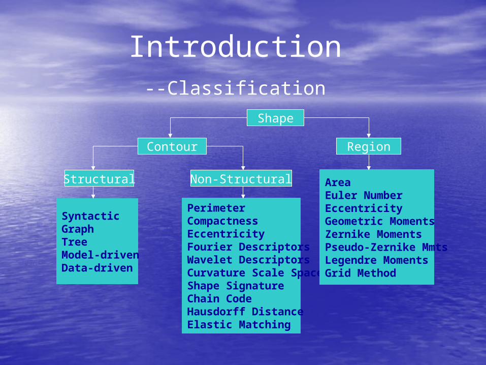
Introduction--Classification

Shape

Contour Region

Structural

SyntacticGraphTreeModel-drivenData-driven

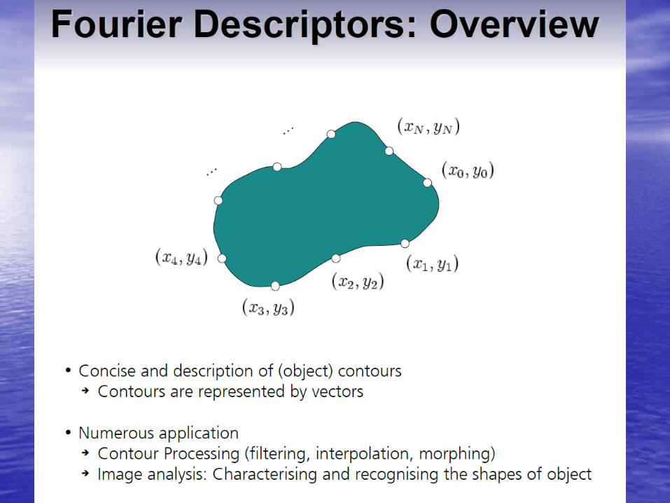
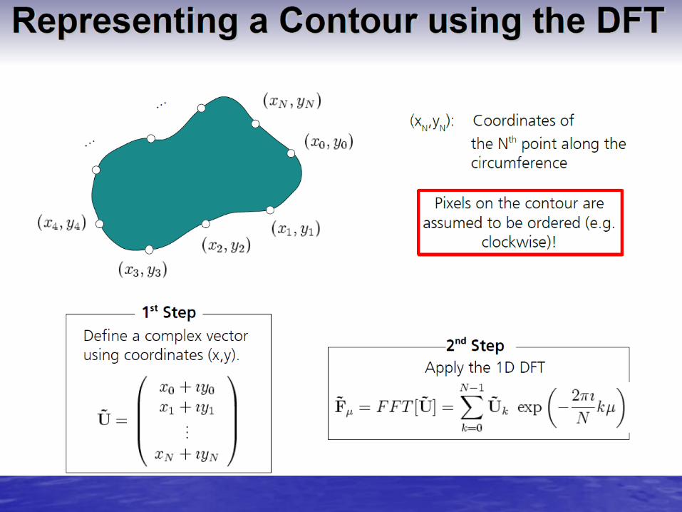
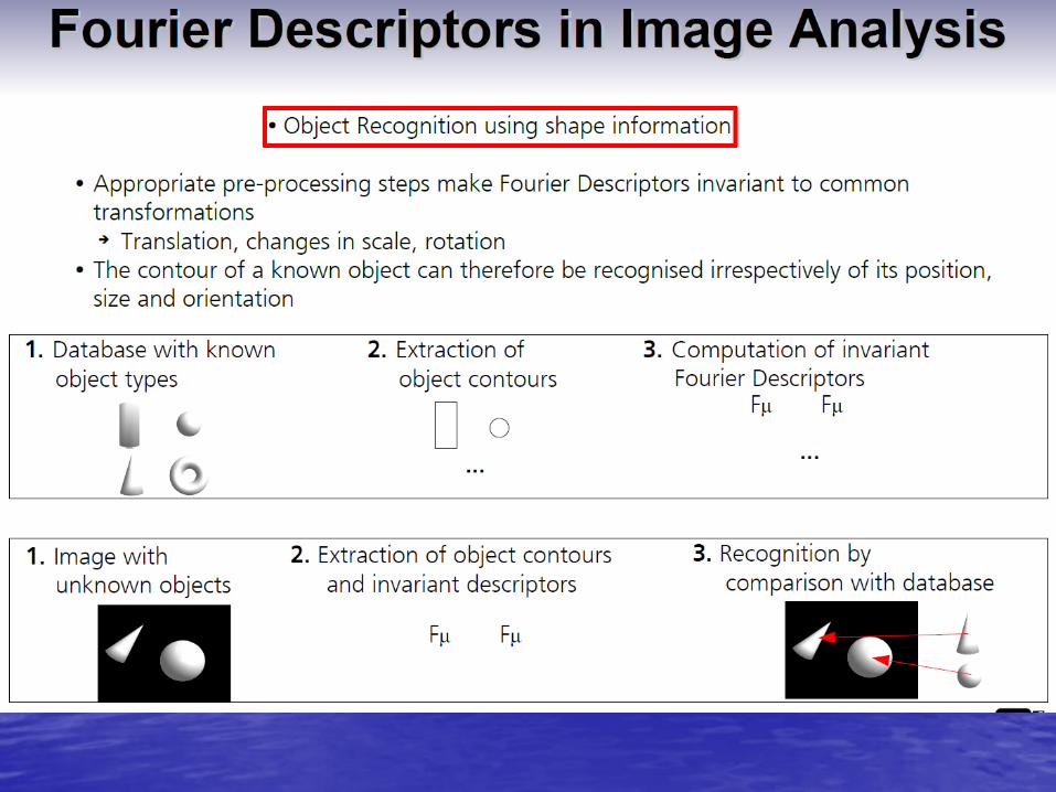
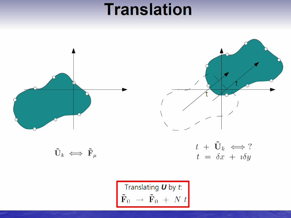
PerimeterCompactnessEccentricityFourier DescriptorsWavelet DescriptorsCurvature Scale SpaceShape SignatureChain CodeHausdorff DistanceElastic Matching

Non-Structural AreaEuler NumberEccentricityGeometric MomentsZernike MomentsPseudo-Zernike MmtsLegendre MomentsGrid Method

Boundary DescriptorsBoundary Descriptors

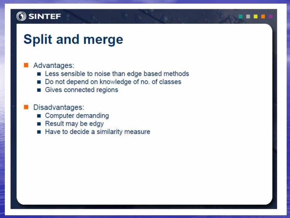
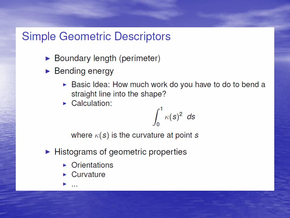
• There are several simple geometric measures that can be useful for describing a boundary. – The length of a boundary: the number of

pixels along a boundary gives a rough approximation of its length.

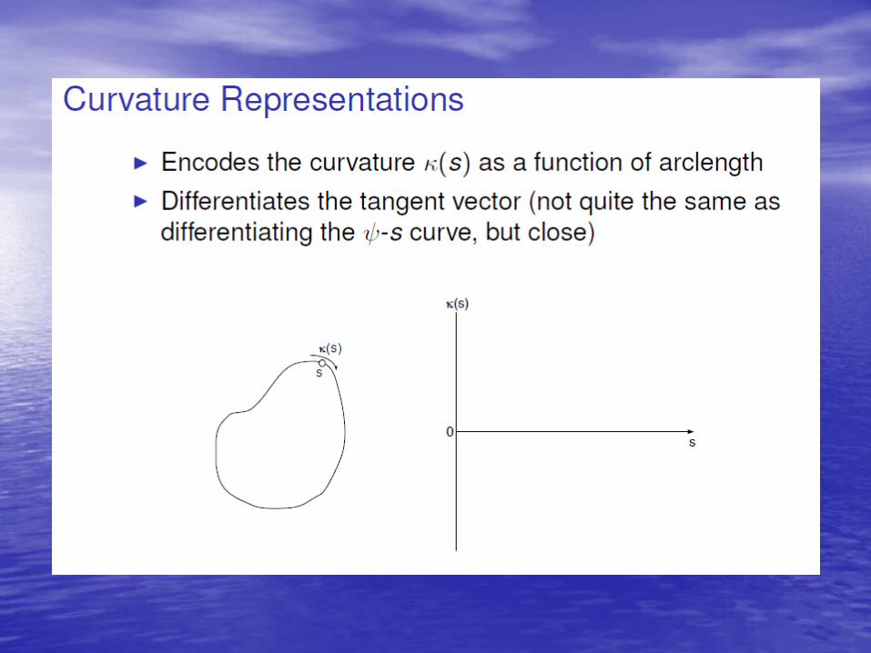
– Curvature: the rate of change of slope• To measure a curvature accurately at a point

in a digital boundary is difficult• The difference between the slops of adjacent

boundary segments is used as a descriptor of curvature at the point of intersection of segments

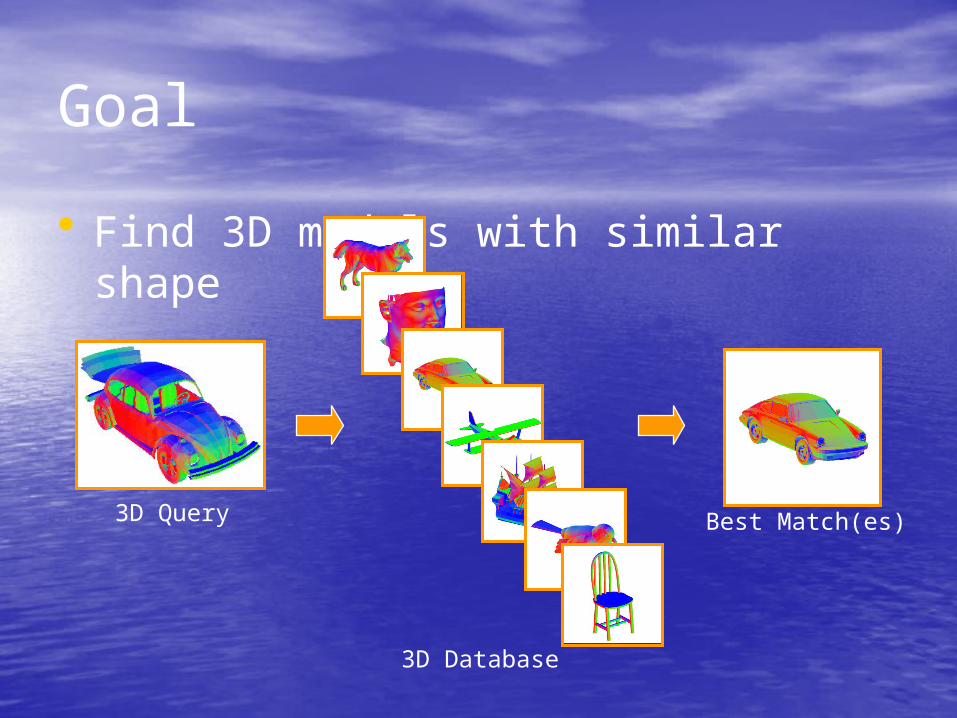
Goal

• Find 3D models with similar shape

3D Query

3D Database

Best Match(es)

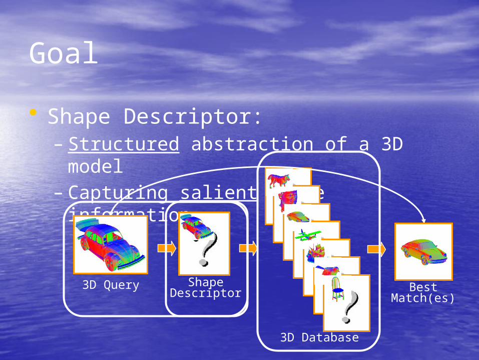
Goal

• Shape Descriptor:– Structured abstraction of a 3D model– Capturing salient shape information

3D Query ShapeDescriptor

3D Database

BestMatch(es)

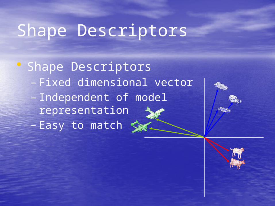
Shape Descriptors

• Shape Descriptors– Fixed dimensional vector– Independent of model representation– Easy to match

Shape Descriptors

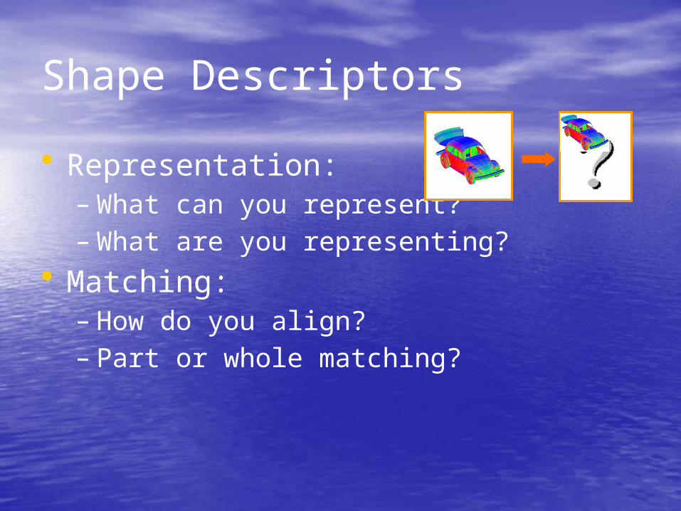
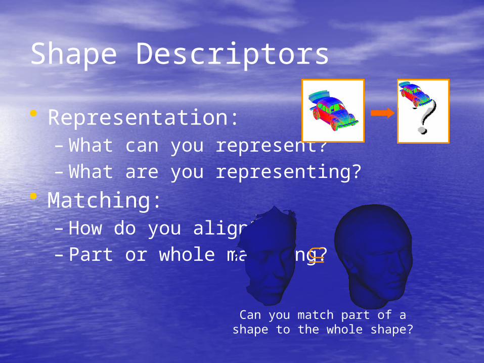
• Representation:– What can you represent?– What are you representing?

• Matching:– How do you align?– Part or whole matching?

Shape Descriptors



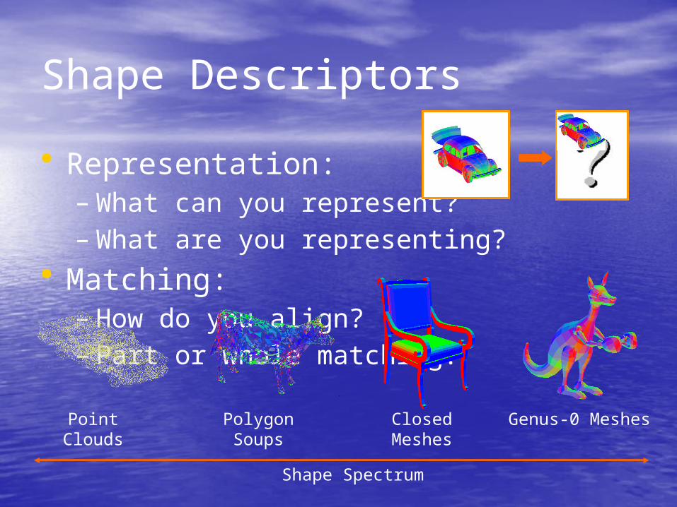
Point Clouds

Polygon Soups

Closed Meshes

Genus-0 Meshes

Shape Spectrum

Shape Descriptors



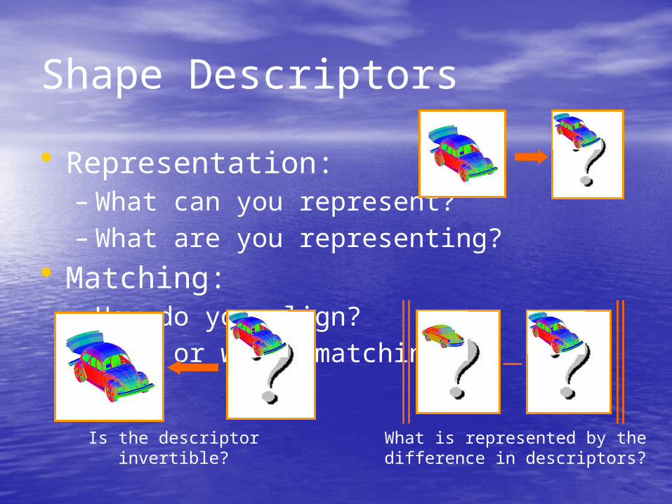
Is the descriptor invertible? What is represented by the difference in descriptors?

Shape Descriptors


• Matching:– How do you align?– Part or whole matching?=

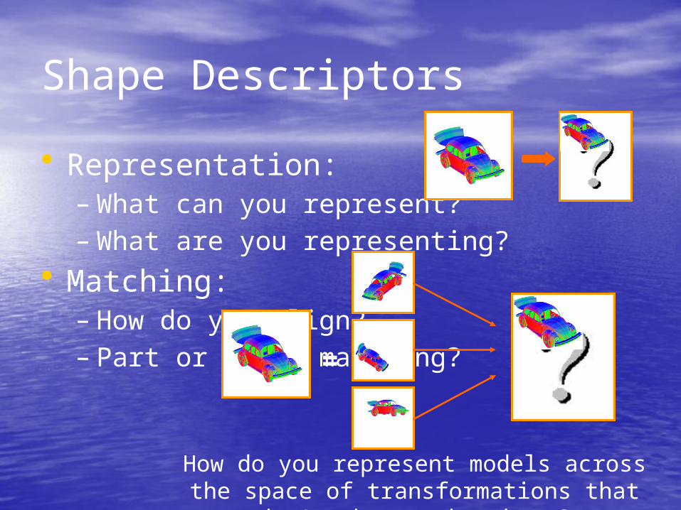
How do you represent models across the space of transformations that don’t change the shape?

Shape Descriptors



Can you match part of a shape to the whole shape?

Outline

Why shape descriptors? How do we represent shapes?

– Volumetric Representations– Surface Representations– View-Based Representations

Conclusion

Volumetric Representations

• Represent models by the volume that they occupy:

Rasterize the models into a binary voxel grid– A voxel has value 1 if it is inside the

model– A voxel has value 0 if it is outside

ModelVoxel Grid

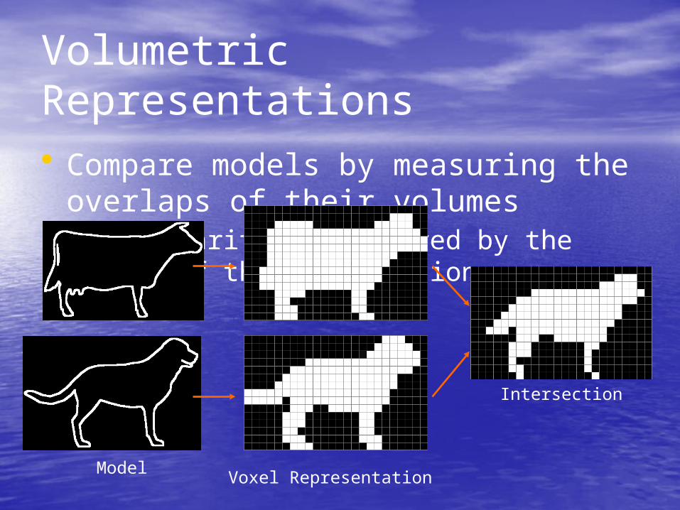
Volumetric Representations

• Compare models by measuring the overlaps of their volumes– Similarity is measured by the size of the

intersection

Intersection

Voxel RepresentationModel

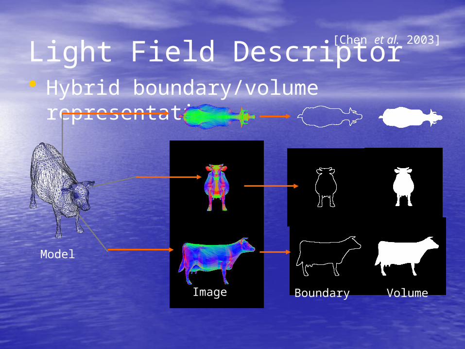
Light Field Descriptor• Hybrid boundary/volume

representation

Model

Image Boundary Volume

[Chen et al. 2003]

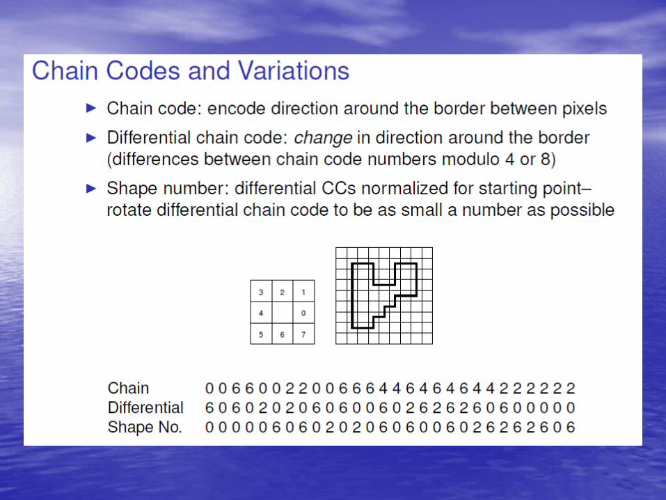
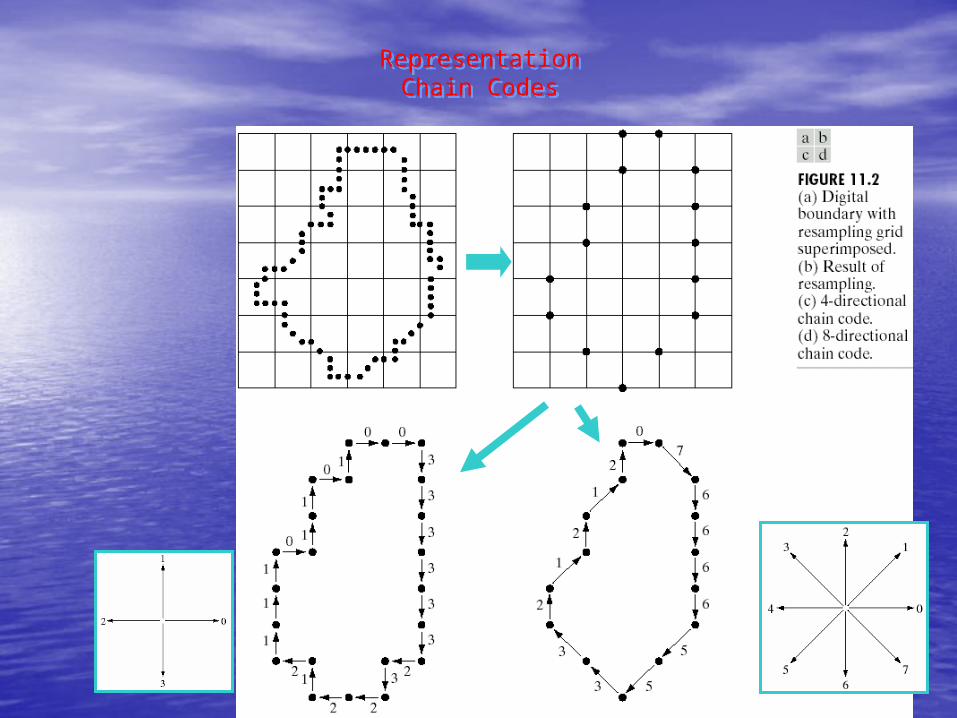
RepresentationChain Codes

RepresentationChain Codes

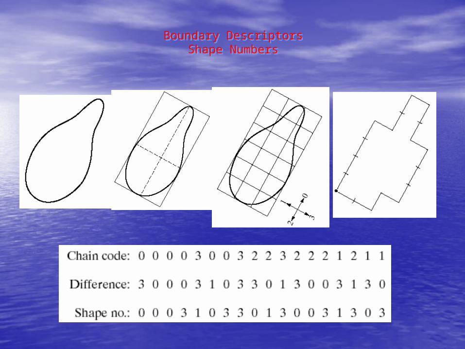
Boundary DescriptorsShape Numbers

Boundary DescriptorsShape Numbers

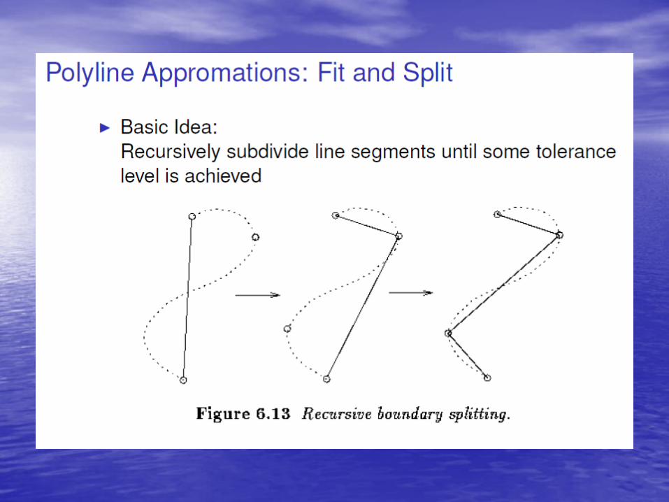
RepresentationPolygonal Approximations


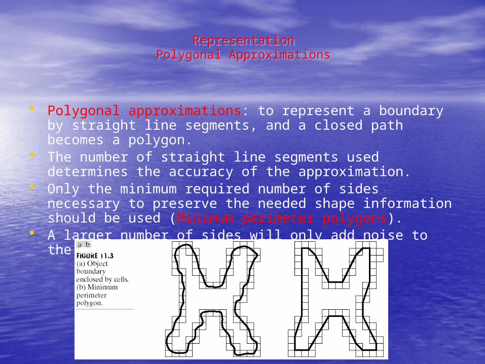
• Polygonal approximations: to represent a boundary by straight line segments, and a closed path becomes a polygon.

• The number of straight line segments used determines the accuracy of the approximation.

• Only the minimum required number of sides necessary to preserve the needed shape information should be used (Minimum perimeter polygons).

• A larger number of sides will only add noise to the model.

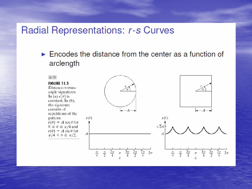
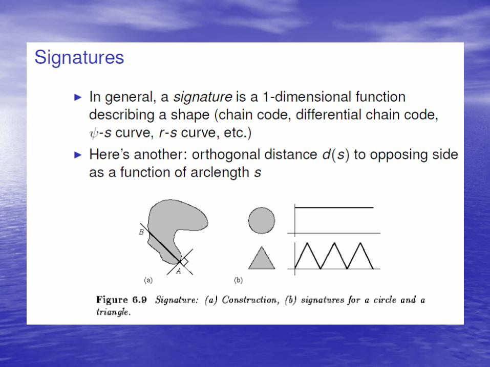
• Signatures are invariant to location, but will depend on rotation and scaling. – Starting at the point farthest from the

reference point or using the major axis of the region can be used to decrease dependence on rotation.

– Scale invariance can be achieved by either scaling the signature function to fixed amplitude or by dividing the function values by the standard deviation of the function.

RepresentationSignature

RepresentationSignature



• Minimum perimeter polygons: (Merging and splitting)– Merging and splitting are often used together to

ensure that vertices appear where they would naturally in the boundary.

– A least squares criterion to a straight line is used to stop the processing.

RepresentationSkeletons

RepresentationSkeletons

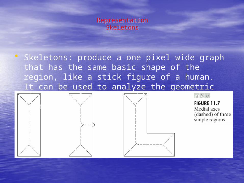
• Skeletons: produce a one pixel wide graph that has the same basic shape of the region, like a stick figure of a human. It can be used to analyze the geometric structure of a region which has bumps and “arms”.

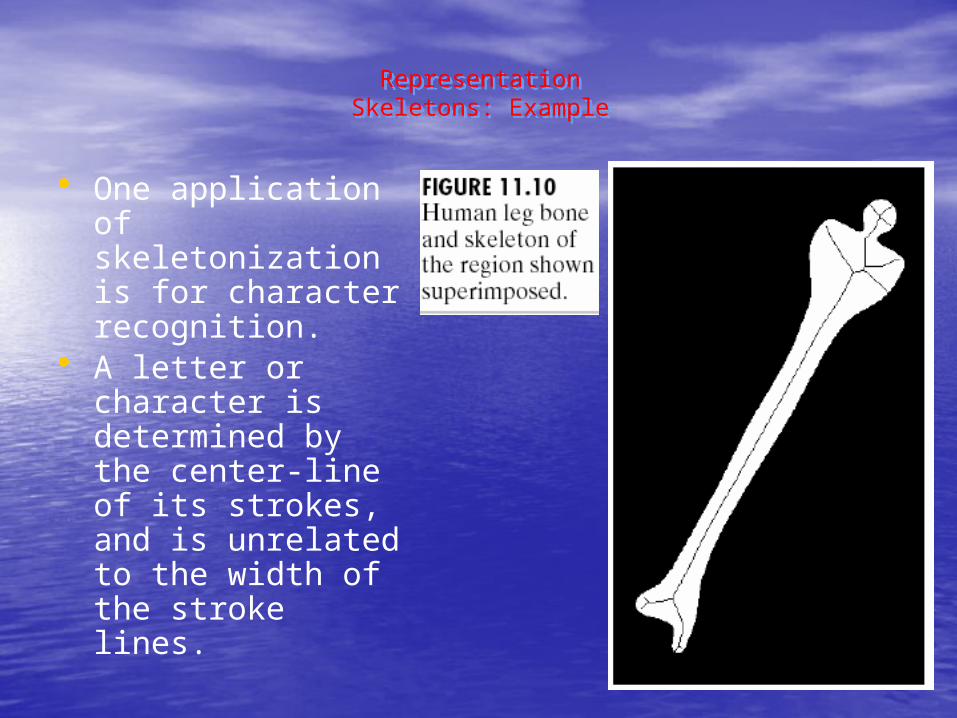
• One application of skeletonization is for character recognition.

• A letter or character is determined by the center-line of its strokes, and is unrelated to the width of the stroke lines.

RepresentationSkeletons: Example

RepresentationSkeletons: Example

Regional DescriptorsTopological DescriptorsRegional Descriptors

Topological Descriptors

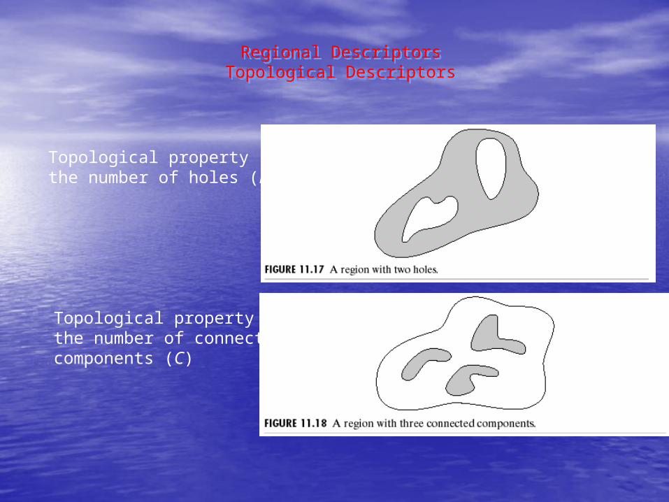
Topological property 1:the number of holes (H)

Topological property 2:the number of connected components (C)



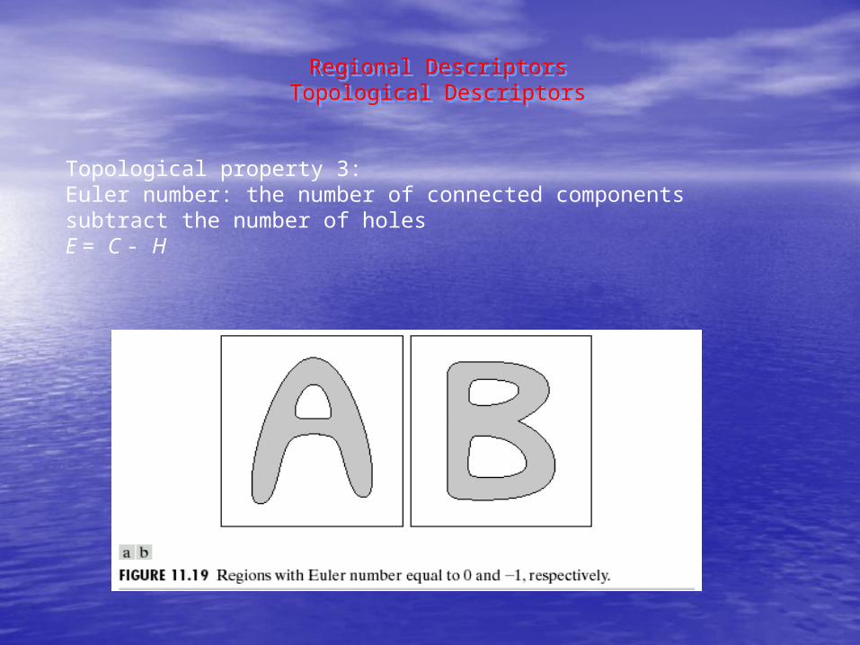
Topological property 3:Euler number: the number of connected components subtract the number of holes E = C - H

E=0 E= -1



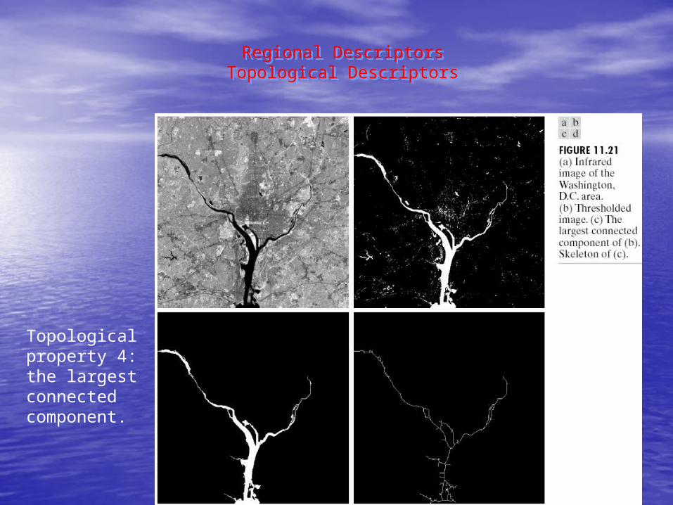
Topological property 4:the largest connected component.

Regional DescriptorsTexture




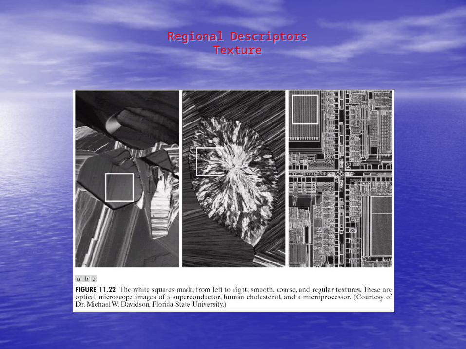
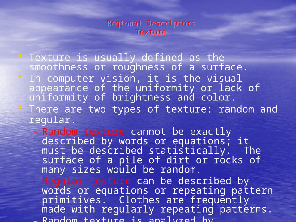
• Texture is usually defined as the smoothness or roughness of a surface.

• In computer vision, it is the visual appearance of the uniformity or lack of uniformity of brightness and color.

• There are two types of texture: random and regular. – Random texture cannot be exactly described

by words or equations; it must be described statistically. The surface of a pile of dirt or rocks of many sizes would be random.

– Regular texture can be described by words or equations or repeating pattern primitives. Clothes are frequently made with regularly repeating patterns.

– Random texture is analyzed by statistical methods.

– Regular texture is analyzed by structural or spectral (Fourier) methods.

Regional DescriptorsStatistical ApproachesRegional Descriptors

Statistical Approaches

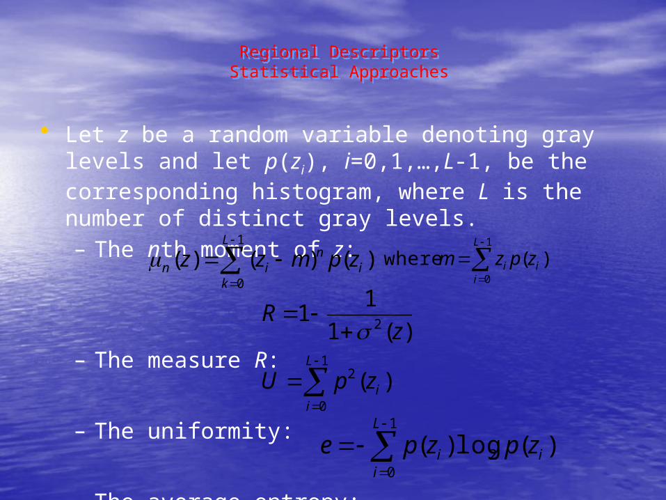
• Let z be a random variable denoting gray levels and let p(zi), i=0,1,…,L-1, be the corresponding histogram, where L is the number of distinct gray levels.– The nth moment of z:

– The measure R:

– The uniformity:

– The average entropy:

1

0

)( whereL

iii zpzm

)(log)( 2

1

0i

L

ii zpzpe

)(1

11

2 zR

1

0

2 )(L

iizpU

1

0

)()()(L

ki

nin zpmzz

Regional DescriptorsStatistical ApproachesRegional Descriptors

Statistical Approaches

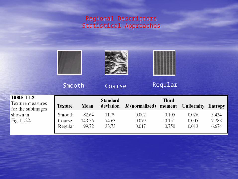
Smooth Coarse Regular

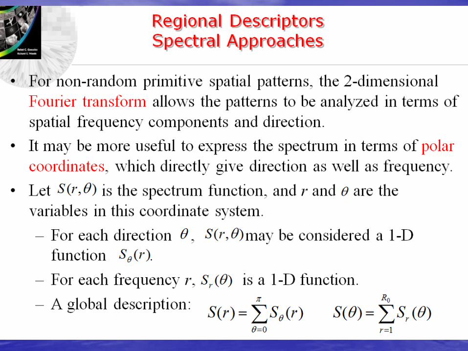
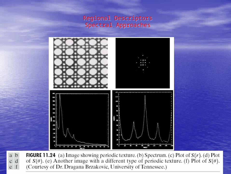
Regional DescriptorsSpectral ApproachesRegional DescriptorsSpectral Approaches

Regional DescriptorsSpectral ApproachesRegional DescriptorsSpectral Approaches

Regional DescriptorsMoments of Two-Dimensional Functions


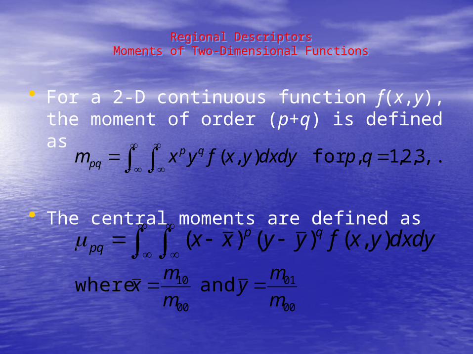
• For a 2-D continuous function f(x,y), the moment of order (p+q) is defined as

• The central moments are defined as

,...3,2,1,for ),(

qpdxdyyxfyxm qp

pq

dxdyyxfyyxx qp

pq ),()()(

00

01

00

10 and wherem

my

m

mx



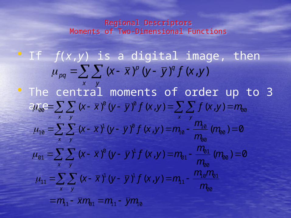
• If f(x,y) is a digital image, then

• The central moments of order up to 3 are

x y

qppq yxfyyxx ),()()(

0000

00 ),(),()()( myxfyxfyyxxx yx y

0)(),()()( 0000

1010

0110 m

m

mmyxfyyxx

x y

0)(),()()( 0000

0101

1001 m

m

mmyxfyyxx

x y

10110111

00

011011

1111

),()()(

mymmxm

m

mmmyxfyyxx

x y



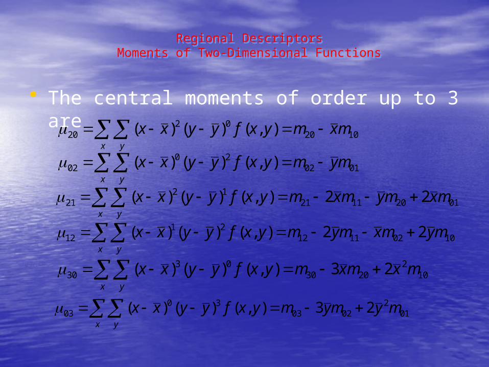
• The central moments of order up to 3 are

102002

20 ),()()( mxmyxfyyxxx y

010220

02 ),()()( mymyxfyyxxx y

0120112112

21 22),()()( mxmymxmyxfyyxxx y

1002111221

12 22),()()( mymxmymyxfyyxxx y

102

203003

30 23),()()( mxmxmyxfyyxxx y

012

020330

03 23),()()( mymymyxfyyxxx y



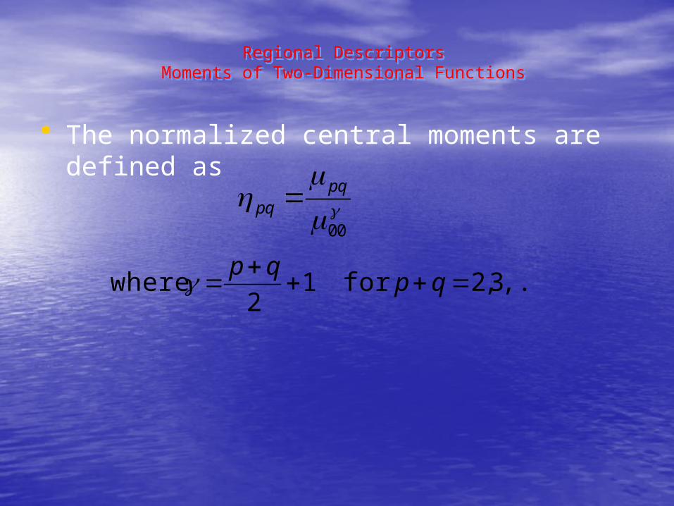
• The normalized central moments are defined as

00

pqpq

,....3,2for 12

where

qpqp



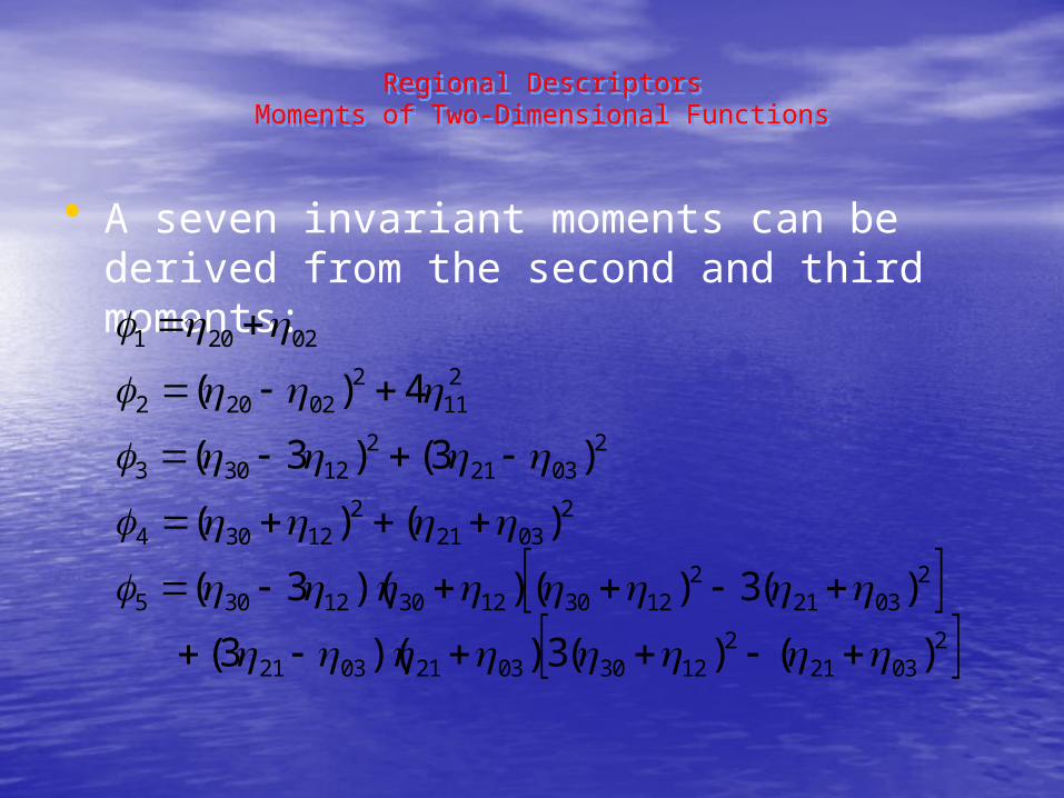
• A seven invariant moments can be derived from the second and third moments:

2

03212

123003210321

20321

21230123012305

20321

212304

20321

212303

211

202202

02201

)()(3))(3(

)(3)())(3(

)()(

)3()3(

4)(



•

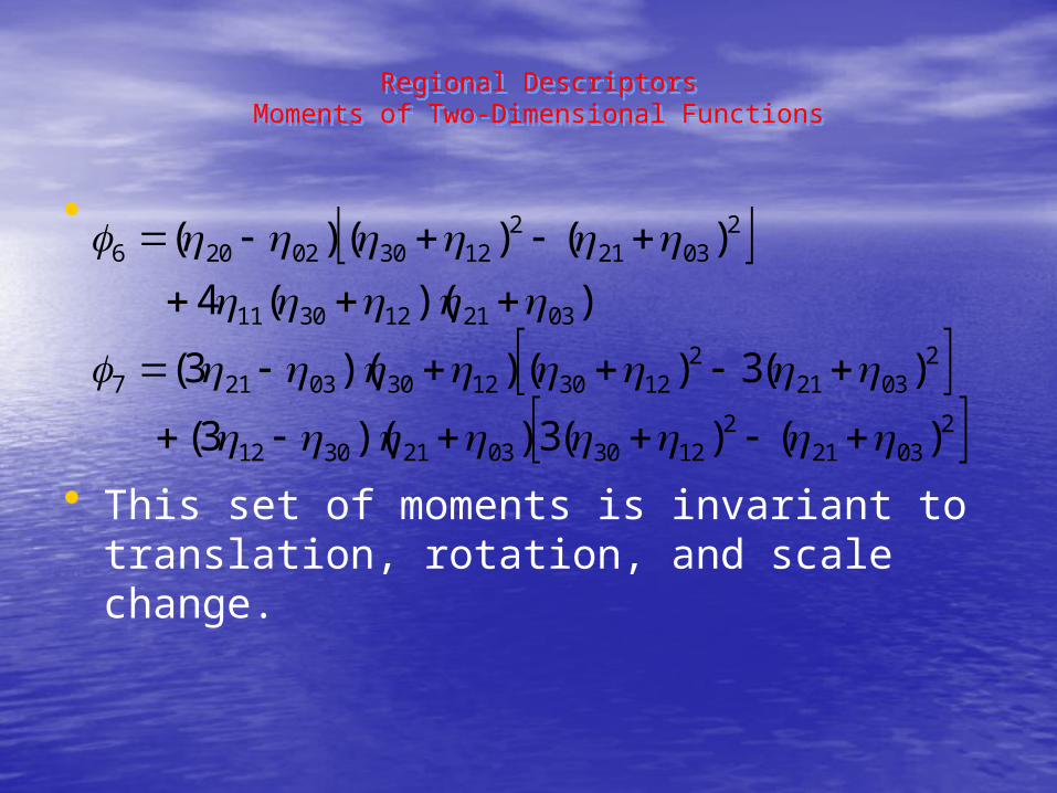
• This set of moments is invariant to translation, rotation, and scale change.

2

03212

123003213012

20321

21230123003217

0321123011

20321

2123002206

)()(3))(3(

)(3)())(3(

))((4

)()()(



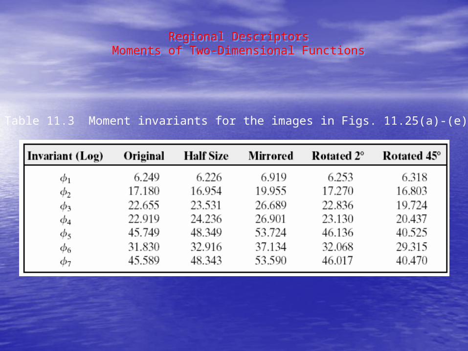
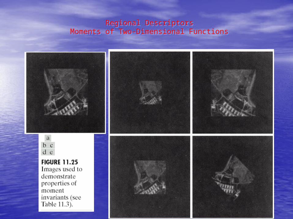
Table 11.3 Moment invariants for the images in Figs. 11.25(a)-(e).



The End

Documents

Introduction --Classification Shape ContourRegion Structural Syntactic Graph Tree Model-driven Data-driven Perimeter Compactness Eccentricity