Introduction - cs.columbia.edu

TOTAL EMBEDDING DISTRIBUTIONS OF CIRCULAR LADDERS

YICHAO CHEN, JONATHAN L. GROSS, AND TOUFIK MANSOUR

Abstract. The total embedding polynomial of a graph G is the bivariate polynomial

IG(x, y) =∞∑

i=0

aixi +

∞∑

j=1

bjyj

where ai is the number of embeddings, for i = 0, 1, . . ., into the orientable surface Si, and bj isthe number of embeddings, for j = 1, 2, . . ., into the non-orientable surface Nj . The sequence{ai(G)|i ≥ 0}

⋃{bj(G)|j ≥ 1} is called the total embedding distribution of the graph G; it is

known for relatively few classes of graphs, compared to the genus distribution {ai(G)|i ≥ 0}.The circular ladder graph CLn is the Cartesian product K22Cn of the complete graph ontwo vertices and the cycle graph on n vertices. In this paper, we derive a closed formula forthe total embedding distribution of circular ladders.

1. Introduction

Genus distributions of graphs have frequently been calculated in the past quarter-century, sincethe topic was inaugurated by Gross and Furst [7]. The contributions include [1, 6, 8, 10, 11, 14,20, 21, 22, 23] and [25]. Quite recently, Gross [12] has derived a quadratic-time algorithm for anyclass of graphs of fixed treewidth and bounded degree, which yields a system of simultaneousrecurrences, but no closed formulas. Total embedding distributions are known for somewhatfewer classes of graphs. Chen, Gross and Rieper [2] computed total embedding distributionsfor necklaces of type (r, 0), closed-end ladders, and cobblestone paths. Kwak and Shim [15]computed it for bouquets of circles and dipoles. Also recently, Chen, Ou and Zou [4] obtainedan explicit formula for the total embedding distributions of Ringel ladders.

Our concern in this paper is circular ladders. McGeoch [18] derived an explicit formula for thegenus distributions of circular ladders and for Mobius ladders (and Li [16, 17] has re-calculatedthem). Yang and Liu [26] counted the embeddings of circular ladders and Mobius ladders inthe projective plane and in the Klein bottle. In this paper, we derive an explicit formula for thetotal embedding distributions of circular ladders, with the aid of Mohar’s overlap matrix [19]and of the Chebyshev polynomials of the second kind.

It is assumed that the reader is at least somewhat familiar with the basics of topological graphtheory, as found in Gross and Tucker [9]. All graphs considered in this paper are connected.A graph G = (V (G), E(G)) is permitted to have loops and multiple edges. A surface is acompact 2-dimensional manifold, without boundary. In topology, surfaces are classified into

2000 Mathematics Subject Classification. Primary: 05C10; Secondary: 30B70, 42C05.Key words and phrases. graph embedding; total embedding distribution; circular ladders; overlap matrix;

Chebyshev polynomials.The work of the first author was partially supported by NNSFC under Grant No. 10901048 and Young

Teachers in Hunan University Fund Project.

1

2 YICHAO CHEN, JONATHAN L. GROSS, AND TOUFIK MANSOUR

the orientable surfaces Sg, with g handles (g ≥ 0), and the non-orientable surfaces Nk, with k

crosscaps (k > 0). The graph embeddings under discussion here are cellular embeddings. Forany spanning tree of a graph G, the number of co-tree edges is called the Betti number of G, orthe cycle rank of G, and is denoted by β(G).

1.1. Background. A rotation at a vertex v of a graph G is a cyclic ordering of all the edge-ends(or equivalently, the half-edges) incident with v. A pure rotation system ρ of a graph G is thecollection of rotations at all the vertices of G. An embedding of G into an orientable surface S

induces a pure rotation system as follows:

the rotation of the edge-ends at vertex v is the cyclic permutation correspondingto the order in which the edge-ends are encountered in an orientation-preservingtour around v.

Conversely, by the Heffter-Edmonds principle, every rotation system induces a unique embedding(up to homeomorphism) of G into some oriented surface S. The bijectivity of this correspondenceimplies that the total number of oriented embeddings is

∏

v∈G(dv − 1)!, where dv is the degreeof vertex v.

A general rotation system for a graph G is a pair (ρ, λ), where ρ is a pure rotation system andλ is a mapping E(G) → {0, 1}. The edge e is said to be twisted (respectively, untwisted) ifλ(e) = 1 (respectively, λ(e) = 0). It is well-known that every oriented embedding of a graph G

can be described uniquely by a general rotation system (ρ, λ) with λ(e) = 0, for all e ∈ E(G).

1.2. Total embedding polynomial. By allowing the parameter λ to take non-zero values,we can describe the non-orientable embeddings of a graph G. For any fixed spanning tree T ,a T -rotation system (ρ, λ) of G is a general rotation system (ρ, λ) such that λ(e) = 0, for alle ∈ E(T ). Any two embeddings of G are considered to be the same if their T -rotation systemsare combinatorially equivalent. Let ΦT

G denote the set of all T -rotation systems of G. It isknown that

|ΦTG| = 2β(G)

∏

v∈V (G)

(dv − 1)!

This implies that the number of non-orientable embeddings of G is

(2β(G) − 1)∏

v∈V (G)

(dv − 1)!

Suppose that among these |ΦTG| embeddings of G, there are ai embeddings, for i = 0, 1, . . ., into

the orientable surface Si, and there are bj embeddings, for j = 1, 2, . . ., into the non-orientablesurface Nj . We call the bivariate polynomial

ITG(x, y) =

∞∑

i=0

aixi +

∞∑

j=1

bjyj

the T -distribution polynomial of G.

It should be noted that the T -distribution polynomial is independent of the choice of spanningtree T . Thus, we may define the total embedding polynomial of G as the bivariate polynomialIG(x, y) = I

TG(x, y), for any choice of a spanning tree T . We call the first and second parts of

IG(x, y) the genus polynomial of G and the crosscap number polynomial of G, respectively, andwe denote them by gG(x) =

∑∞

i=0 aixi and fG(y) =

∑∞

i=1 biyi, respectively. Thus, we have

IG(x, y) = gG(x) + fG(y).

TOTAL EMBEDDING DISTRIBUTIONS OF CIRCULAR LADDERS 3

1.3. Overlap matrices. Mohar [19] introduced an invariant that has been used numerous timesin the calculation of graph embedding distributions, starting with [2]. Let T be a spanning treeof a graph G, and let (ρ, λ) be a T -rotation system. Let e1, e2, . . . , eβ(G) be the cotree edgesof T . The overlap matrix of (ρ, λ) is the β(G) × β(G) matrix M = [mij ] over Z2 such that

mij =

1, if i = j and ei is twisted;

1, if i 6= j and the restriction of the underlying pure rotation systemto the subgraph T + ei + ej is nonplanar;

0, otherwise.

When the restriction of the underlying pure rotation system to the subgraph T + ei + ej isnonplanar, we say that edges ei and ej overlap. The power of the overlap matrix is indicatedby this theorem.

Theorem 1.1 (Mohar [19]). Let (ρ, λ) be a general rotation system for a graph, and let M bethe overlap matrix with respect to any spanning tree. Then the rank of M equals twice the genusof the corresponding embedding surface, if that surface is orientable, and it equals the crosscapnumber otherwise. It is independent of the choice of a spanning tree.

2. Overlap matrices of circular ladders

The circular ladder graph CLn is the graph Cartesian product Cn×K2, whereK2 is the completegraph on two nodes and Cn is the cycle graph on n nodes. Figure 1 depicts the circular laddergraph CL4.

Figure 1. The circular ladder CL4

2.1. Gustin’s represention of rotation systems for cubic graphs. For drawing a planarrepresentation of a rotation system on a cubic graph, we adopt the graphic “nomogram” (ter-minology due to Youngs) introduced by Gustin [13], and used extensively by Ringel and Youngs(see [24]) in their solution to the Heawood map-coloring problem. A trivalent vertex has twopossible rotations. There are two possible cyclic orderings of each trivalent vertex. Under thisconvention, we color a vertex black if the rotation of the edge-ends incident on it is clockwise,and we color it white if the rotation is counterclockwise. We call any drawing of a graph that usesthis convention to indicate a rotation system a Gustin representation of that rotation system.

In a Gustin nomogram, an edge is called matched if it has the same color at both endpoints;otherwise, it is called unmatched. In Figure 2, we have indicated our choice of a spanning tree fora generic circular ladder CLn+1 by thicker lines, so that the cotree edges are e, f, e1, e2, · · · , en,and our partial choice of rotations at the vertices.


v1 v2 v3 v4 vn−1 vn vn+1

u1 u2 u3 u4 un−1 un un+1

b1 b2 b3 b4 · · · bn bn+1

a1 a2 a3 · · · an−1 an

e1 e2 e3 · · · en−1 en

e

f

1

Figure 2. A Gustin nomogram for a circular ladder

2.2. Overlap matrices for circular ladder graphs. In the Gustin nomogram of Figure 2,we observe the following properties:

Property 2.1. Two cotree edges e and ei overlap if and only if the edge ai is unmatched, fori = 2, 3, · · · , n− 1.

Property 2.2. Two cotree edges f and ei overlap if and only if the edge ai is unmatched, fori = 1, 2, · · · , n.Property 2.3. Two cotree edges ei and ei+1 overlap if and only if the edge bi+1 is unmatched,for i = 1, 2, · · · , n− 1.

Property 2.4. The cotree edges e and e1 overlap if and only if the vertices u2 and v1 are coloreddifferently.

Property 2.5. The cotree edges e and en overlap if and only if the vertices un and vn+1 arecolored differently.

It follows that the overlap matrix of CLn+1 has this form, where xi, yj , zk ∈ Z2:

Mc,x,y,X,Y,Zn+2 =

xe c x z2 z3 · · · zn−1 y

c xf z1 z2 z3 · · · zn−1 znx z1 x1 y1z2 z2 y1 x2 y2 0

z3 z3 y2 x3. . .

......

. . .. . . yn−2

zn−1 zn−1 0 yn−2 xn−1 yn−1

y zn yn−1 xn

Note that xe = 1 if and only if the edge e is twisted, and that xf = 1 if and only if the edge f

is twisted. Also note that• xi = 1 if and only if the edge ei is twisted, for all i = 1, 2, . . . , n;• yj = 1 if and only if bj+1 is unmatched, for all j = 1, 2, . . . , n− 1; and• zk = 1 if and only if ak is unmatched, for all k = 1, 2, . . . , n.

Moreover, we have x = 1 if and only if the colors of vertices v1 and u2 are different, and we havey = 1 if and only if the colors of vertices vn+1 and un are different. Furthermore, we have


Property 2.6. The constant c = 1 (i.e., edges e and f overlap) if and only if the number ofvalues of z1, z2, . . . , zn equal to 1 is odd.

Proof. The proof is by induction on n. Note that the edges e and f overlap if only if the verticesof u1 and un+1 are colored differently. For n = 1, this means the edge a1 unmatched, this isequivalent to saying z1 = 1.

Suppose that this is true for n = k and the number of values of z1, z2, . . . , zk equal to 1 is2m+ 1, (2m+ 1 ≤ n). It should be noted that the vertex set of u1, u2, . . . , uk+1 of CLk+1 canbe obtained by inserting a vertex u between ui and ui+1, i = 1, . . . , k − 1 of CLk and relabelthem. If the coloring of ui and ui+1 are differently, no matter what assignment of colors to u,the number of values of z1, z2, . . . , zk+1 equal to 1 also equals 2m+1. Otherwise the coloring ofui and ui+1 are the same (black or white), the number of values of z1, z2, . . . , zk+1 equal to 1equals 2m+1 or 2m+3 according to the assignment of colors of u is the same or different fromthat of ui and ui+1 respectively. �

Property 2.7. For each fixed matrix of the form Mc,x,y,X,Y,Zn+2 , there are exactly two different

T -rotation systems of the circular ladder CLn for which Mc,x,y,X,Y,Zn+2 is the overlap matrix.

Proof. Given a matrix Mc,x,y,X,Y,Zn+2 , the values of x, y, z1, z2, · · · , zn and y1, y2, · · · , yn−1 are

determined.

z1 = 0: If the vertex u1 is black, then u2 is also black, by Property 2.2. Alternatively, if thevertex u1 is white, then the color of u2 is also white. In either case, since the values ofx, y, z2, · · · , zn and y1, y2, · · · , yn−1 are given, all the colors of v1, v2, u2, · · · , vn+1, un+1

are determined, by Properties 2.2, 2.3, 2.4, 2.5, and 2.6. That is, all the rotations atvertices of CLn are determined.

z1 = 1: The proof is similar to the case z1 = 0. Details are omitted.�

We define (with x and y ranging over Z2)

(1) An+2 as the set of all matrices over Z2 of the form Mc,x,y,X,Y,Zn+2 ;

(2) An+2(z) =∑n+2

j=0 An+2(j)zj as the rank-distribution polynomial of the set An+2, where

An+2(j) denotes the number of matrices in An+2 of rank j, that is, the number of overlapmatrices of rank j for general rotation systems for the circular ladder CLn;

(3) Bn+2 as the set of all matrices of the form Mc,x,y,0,Y,Zn+2 ; and

(4) Bn+2(z) =∑n+2

j=0 Bn+2(j)zj as the rank-distribution polynomial of the set Bn+2, where

Bn+2(j) denotes the number of matrices in Bn+2 of rank j, that is, the number ofoverlap matrices of rank j for pure rotation systems for the circular ladder CLn.

It should be mentioned that the orientable case is precisely when X is identically 0.

In a matrix of the form Mc,x,y,X,Y,Zn+2 , suppose that we first add the second row to the first row

and next add the second column to the first column. Without changing the rank of the matrix,this produces a matrix of the following form:


xe c+ xf x 0 · · · 0 0 y

c+ xf xf z1 z2 · · · zn−2 zn−1 znx z1 x1 y1

0 z2 y1 x2. . . 0

......

. . .. . .

0 zn−2 0 yn−2

0 zn−1 0 yn−2 xn−1 yn−1

y zn yn−1 xn

For each single specific choice xy ∈ {00, 01, 10, 11}, we define

(1) Axyn+2 as the set of all matrices over Z2 of the form M

c,x,y,X,Y,Zn+2 ;

(2) Axyn+2(z) =

∑n+2j=0 A

xyn+2(j)z

j as the rank-distribution polynomial of the set Axyn+2;

(3) Bxyn+2 as the set of all matrices of the form M

c,x,y,0,Y,Zn+2 ; and

(4) Bxyn+2(z) =

∑n+2j=0 B

xyn+2(j)z

j as the rank-distribution polynomial of the set Bin+2.

Clearly, we have the following property.

Property 2.8. For all n ≥ 1,

An+2(z) =∑

xy=00,01,10,11

Axyn+2(z) and Bn+2(z) =

∑

xy=00,01,10,11

Bxyn+2(z).

3. Rank-distribution polynomials of some ladder graphs

We recall that the n-rung closed-end ladder Ln can be obtained from the graphical cartesianproduct of an n-vertex path with the complete graphK2 by doubling both its end edges. Figure 3illustrates the 4-rung closed-end ladder L4.

Figure 3. The 4-rung closed-end ladder L4

We recall also that the Ringel ladder Rn, can be formed by subdividing the end-rungs of theclosed-end ladder, Ln, and then adding an edge between these two new vertices. Figure 4 showsthe Ringel ladder R4.

Figure 4. The Ringel ladder R4


3.1. Rank-distribution polynomial for Ringel ladders. For the vectorsX = (x0, x1, . . . , xn),Y = (y1, y2, . . . , yn−1), and Z = (z1, z2, . . . , zn), with xi, yj , zk ∈ Z2, we define the matrices

(1) MX,Yn =

x1 y1y1 x2 y2 0

y2 x3 y3. . .

. . .. . .

0 yn−2 xn−1 yn−1

yn−1 xn

and

(2) MX,Y,Zn+1 =

x0 z1 z2 z3 . . . zn−1 znz1 x1 y1z2 y1 x2 y2 0

z3 y2 x3. . .

.... . .

. . . yn−2

zn−1 0 yn−2 xn−1 yn−1

zn yn−1 xn

.

As described by [2, 4], every overlap matrix of the closed-end ladder Ln−1 has the form MX,Yn+1 ,

and every overlap matrix of the Ringel ladder Rn−1 has the form MX,Y,Zn+1 . (Note that the

subscripts of Rn−1 and MX,Y,Zn+1 differ by two.) Now we further define

(1) Rn as the set of all matrices over Z2 of the form MX,Y,Zn ;

(2) Cn(j) as the number of overlap matrices for Rn that are of rank j;

(3) Rn(z) =∑n+1

j=0 Cn(j)zj as the rank-distribution polynomial of the set Rn; and

(4) Ln(z) as the rank-distribution polynomial of the overlap matrices of the closed-endladder Ln−1.

In the calculations of this section, we use the following two previously derived results:

Theorem 3.1. [3] The polynomial Ln(z) satisfies the recurrence relation

Ln(z) = (1 + 2z)Ln−1(z) + 4z2Ln−2(z)

with the initial conditions L1(z) = 1 + z and L2(z) = 4z2 + 3z + 1. Moreover, the generatingfunction L(t; z) =

∑

n≥1 Ln(z)tn is given by the formula

L(t; z) =t(1 + z + 2z2t)

1− t− 2tz − 4z2t2. �

Theorem 3.2. [4] The polynomial Rn(z) (n ≥ 3) satisfies the recurrence relation

Rn+1(z) = (4z + 1)Rn(z) + 16z2Rn−1(z) + 2nz2Ln−1(z).

with the initial condition R2(z) = 4z2+3z+1 and R3(z) = 28z3+28z2+7z+1. Moreover, thegenerating function R(t; z) =

∑

n≥2 Rn(z)tn is given by

R(t; z) =t2(1 + 3z + 4z2 − 2(1 + 5z + 4z2 + 2z3)t− 16z2(2 + 6z + 5z2)t2 − 128z4(1 + z)t3)

(1 − 2t− 4tz − 16z2t2)(1− t− 4tz − 16z2t2).

�


Here we split the enumeration into even and odd parts:

(1) let MX,Y,Zeven

n+1 be the number of matrices of the form MX,Y,Zn+1 and such that the sum of

the elements of the vector Z is even;

(2) let MX,Y,Zodd

n+1 be the number of matrices of the form MX,Y,Zn+1 with x0 = 0 and such that

the sum of the elements of the vector Z is odd;

(3) let MX,Y,Zeven

n+1 be the number of matrices of the form MX,Y,Zn+1 with x0 = 0 and such

that the sum of the elements of the vector Z is even;

(4) let MX,Y,Zodd,1n+1 be the number of matrices of that form with x0 = 1 and such that the

sum of the elements of Z is odd;

(5) let REn+1(z) be the rank-distribution polynomial over the set MX,Y,Zeven

n+1 ;

(6) let ROn+1(z) be the rank-distribution polynomial over the set MX,Y,Zodd

n+1 ;

(7) let RE,0n+1(z) be the rank-distribution polynomial over the set MX,Y,Zeven,0

n+1 ; and

(8) let RO,1n+1(z) be the rank-distribution polynomial over the set MX,Y,Zodd,1

n+1 .

Lemma 3.3. The polynomial RE,0n (z) + RO,1

n (z) (n ≥ 4) satisfies the recurrence

RE,0n+1(z) + R

O,1n+1(z) = (2z + 1)

(

RE,0n (z) + R

O,1n (z)

)

+ zRn(z) + 8z2Rn−1(z) + 2n−1z2Ln−1(z)

with initial condition RE,03 (z) + R

O,13 (z) = 1 + 5z + 14z2 + 12z3 (where Rn−1(z) and Ln−1(z)

are the rank-distribution polynomials of the overlap matrices of the Ringel ladder Rn−3 and ofthe closed-end ladder Ln−2, respectively).

Proof. We first prove the following claim.

Claim 1: The polynomial RE,0n (z) (n ≥ 4) satisfies the recurrence

RE,0n+1(z) = R

E,0n (z) + z

(

RE,0n (z) + R

O,1n (z)

)

+ zREn (z)

+ 4z2R0n−1(z) + 2z2Rn−1(z) + 2n−2z2Ln−1(z).

with initial condition RE,03 (z) = 1 + 3z + 8z2 + 4z3.

We analyze the form (see Equation (2)) of the overlap matrix MX,Y,Zn+1 into possible cases.

(1) Case 1: xn = 1.• subcase 1: yn−1 = 1. We first add the last row to row n and then add the lastcolumn to column n. The resulting matrix has the following form.

0 z1 z2 · · · zn−2 zn−1 + zn znz1 x1 y1

z2 y1 x2. . . 0

.... . .

. . .

zn−2 xn−2 yn−2

zn−1 + zn 0 yn−2 xn−1 0zn 0 1

If zn = 0, this matrix contributes a term zRE,0n (z) to the polynomial RE,0

n+1(z).

Otherwise zn = 1, and it contributes a term zRE,1n (z)

• subcase 2: yn−1 = 0. As seen by a discussion similar to that for subcase 1, thissubcase contributes a term zRE,0

n (z) + zRO,1n (z).


(2) Case 2: xn = 0. This case, given by the following matrix, has four subcases.

(3)

0 z1 z2 · · · zn−2 zn−1 znz1 x1 y1

z2 y1 x2. . . 0

.... . .

. . .

zn−2 xn−2 yn−2

zn−1 0 yn−2 xn−1 1zn 1 0

• subcase 1: yn−1 = 1, zn = 0. No matter what the values of yn−2, zn−1 and xn−1,we can transform the above matrix to the following form, with no change of rank.

0 z1 z2 · · · zn−2 0 0z1 x1 y1

z2 y1 x2. . . 0

.... . .

. . .

zn−2 xn−2

0 0 0 0 10 1 0

There are four different combinations of values for the variables yn−2 and xn−1.

When zn−1 = 0, this matrix contributes 4z2RE,0n−1(z) to the polynomial RE,0

n+1(z).

When zn−1 = 1, it contributes 4z2RO,0n−1(z). Since R

O,0n−1(z) + R

E,0n−1(z) = R0

n−1(z),

this case contributes in all a term 4z2R0n−1(z).

• subcase 2: yn−1 = 1, zn = 1. We add row n to the first row then add column n tothe first column, as indicated by this matrix.

xn−1 z1 z2 · · · zn−2 + yn−2 zn−1 + xn−1 0z1 x1 y1

z2 y1 x2. . . 0

.... . .

. . .

zn−2 + yn−2 xn−2 yn−2

zn−1 + xn−1 0 yn−2 xn−1 10 1 0

If xn−1 = 0, this case contributes 2z2R0n−1(z) to the polynomial RE,0

n+1(z). Other-

wise xn−1 = 1, and this case contributes 2z2R1n−1(z).

• subcase 3: yn−1 = 0, zn = 0. This case also contributes RE,0n (z) to the polynomial

RE,0n+1(z).


• subcase 4: yn−1 = 0, zn = 1. No matter what values of z1, z2, . . . , zn−1 occur, wecan transform Matrix (3) into the following form.

0 0 0 · · · 0 0 10 x1 y1

0 y1 x2. . . 0

.... . .

. . .

0 xn−2 yn−2

0 0 yn−2 xn−1 01 0 0

Since there are 2n−2 possible choices of values for z1, z2, . . . , zn−1 with an even sum,

this subcase contributes 2n−2z2Ln−1(z) to the polynomial RE,0n+1(z).

By a similar analysis, we can substantiate a second claim.

Claim 2: The polynomial RO,1n (z) satisfies this recursion, for (n ≥ 4):

RO,1n+1(z) = R

O,1n (z) + z

(

RO,1n (z) + R

E,0n (z)

)

+ zROn (z)

+ 4z2R1n−1(z) + 2z2Rn−1(z) + 2n−2z2Ln−1(z).

with initial conditions RO,13 (z) = 2z + 6z2 + 8z3.

From the above two claims, the lemma follows. �

Proposition 3.4. The generating function R′(t; z) =∑

n≥3(RE,0n (z)+RO,1

n (z))tn has the closedform

t3f(t; z)

(1− 2t− 4tz − 16z2t2)(1 − t− 4tz − 16z2t2)(1 − t− 2tz),

where

f(t; z) = 14z2 + 12z3 + 1 + 5z + (−20z4 − 3− 84z3 − 22z − 63z2)t

+ (2 + 20z + 34z2 − 272z4 − 272z5 − 56z3)t2 − 16z2(8z4 − 43z2 − 20z − 3− 34z3)t3

+ 256z4(1 + 2z)(1 + z)2t4.

Proof. Multiplying the recurrence relation of Lemma 3.3 for the polynomial RE,0n (z) + RO,1

n (z)by tn and then summing over all n ≥ 3, we establish that a closed form for R′(t; z) is given by

t3f(t; z)

(1− 2t− 4tz − 16z2t2)(1 − t− 4tz − 16z2t2)(1 − t− 2tz),

We have used the explicit formulas for the generating functions R(t; z) and L(t; z), as given inTheorem 3.1 and Theorem 3.2, respectively. �


3.2. Expressing polynomials for circular ladders as a combination of polynomials for

Ringel ladders and closed-end ladders. We are now ready to approach the circular ladders.

Lemma 3.5. The polynomial A01n (z) satisfies this equation for n ≥ 4:

A01n+2(z) = (2z + 1)

(

RE,0n+1(z) + R

O,1n+1(z)

)

+ 2nz2Ln(z)(4)

where Rn+1(z) is the rank-distribution polynomial of the Ringel ladder Rn−1 and Ln(z) is therank-distribution polynomial of the closed-end ladder Ln−1.

Proof. There are two cases.

(1) Case 1: xe = 1. Here the overlap matrix has the following form:

1 xf + c 0 0 · · · 0 0 0xf + c xf z1 z2 · · · zn−2 zn−1 zn

0 z1 x1 y1

0 z2 y1 x2. . . 0

......

. . .. . .

0 zn−2 xn−2 yn−2

0 zn−1 0 yn−2 xn−1 yn−1

0 zn yn−1 xn

• subcase 1: c = 0. When xf = 0, this subcase contributes a term zRE,0n+1(z); when

xf = 1, we add the first row to the second row, and then add the first column to

the second column, to see that this subcase still contributes a term zRE,0n+1(z).

• subcase 2: c = 1. When xf = 1, this subcase contributes a term zRO,1n+1(z); when

xf = 0, we first add the first row to the second row and then add the first column

to the second column, to see that this case still contributes a term zRO,1n+1(z).

(2) Case 2: xe = 0. In this case, the overlap matrix has the following form.


0 z1 x1 y1

0 z2 y1 x2. . . 0

......

. . .. . .

0 zn−2 xn−2 yn−2

0 zn−1 0 yn−2 xn−1 yn−1

0 zn yn−1 xn

• subcase 1: c = 0. When xf = 0, the contributed term is RE,0n+1(z). Otherwise

xf = 1; since there are 2n−1 choices of values of z1, z2, · · · , zn with an even sum,the contributed term is 2n−1z2Ln(z).

• subcase 2: c = 1. When xf = 0, since there are 2n−1 choices of values ofz1, z2, · · · , zn with an odd sum, the contributed term is 2n−1z2Ln(z); otherwise

xf = 1,, and the contributed term is RO,1n+1(z).

�


Lemma 3.6. The polynomial A10n (z) satisfies this equation, for n ≥ 4:

A10n+2(z) = zRn+1(z) + 8z2Rn(z).(5)

where Rn(z) is the rank-distribution polynomial of the Ringel ladder Rn−2.

Proof. We examine the following two cases.

(1) Case 1: xe = 1. In this case, the overlap matrix has the following form.


1 z1 x1 y1

0 z2 y1 x2. . . 0

......

. . .. . .

0 zn−2 xn−2 yn−2

0 zn−1 0 yn−2 xn−1 yn−1

0 zn yn−1 xn

When we add the first row to the third row and add the first column to the third column,the resulting matrix has the following form.

1 xf + c 0 0 · · · 0 0 0xf + c xf z1 + xf + c z2 · · · zn−2 zn−1 zn

0 z1 + xf + c x1 y1

0 z2 y1 x2. . . 0

......

. . .. . .

0 zn−2 xn−2 yn−2

0 zn−1 0 yn−2 xn−1 yn−1

0 zn yn−1 xn

• subcase 1: c = 0. If xf = 0, the contributed term is zRE,0n+1(z). Otherwise xf = 1,

and we first add the first row to the second row, then add the first column to the

second column, to establish that the contributed term is zRO,0n+1(z).

• subcase 2: c = 1. If xf = 0, we first add the first row to the second row, and then

add the first column to the second column. The contributed term is zRE,1n+1(z).

Otherwise xf = 1, and the contributed term is zRO,1n+1(z).

(2) Case 2: xe = 0. In this case, the matrix has the following form.


1 z1 x1 y1

0 z2 y1 x2. . . 0

......

. . .. . .

0 zn−2 xn−2 yn−2

0 zn−1 0 yn−2 xn−1 yn−1

0 zn yn−1 xn


• subcase 1: c = 0. First suppose that xf = 0. There are four different choices ofvalues for the variables x1 and y1. According to the values z1 = 0 or z1 = 1, thiscase contributes a term 4z2RE,0

n (z) or 4z2RO,0n (z). For xf = 1, we first add the

third row to the second row and then add the third column to the second column.The resulting matrix has the following form.

0 0 1 0 · · · 0 0 00 1 + x1 z1 + x1 z2 + y1 · · · zn−2 zn−1 zn1 z1 + x1 x1 y1

0 z2 + y1 y1 x2. . . 0

......

. . .. . .

0 zn−2 xn−2 yn−2

0 zn−1 0 yn−2 xn−1 yn−1

0 zn yn−1 xn

No matter what the values of the variables of x1, y1 and z1, we can transform thatmatrix into the following form.

0 0 1 0 · · · 0 0 00 1 + x1 0 z2 + y1 · · · zn−2 zn−1 zn1 0 0 0

0 z2 + y1 0 x2. . . 0

......

. . .. . .

0 zn−2 xn−2 yn−2

0 zn−1 0 yn−2 xn−1 yn−1

0 zn yn−1 xn

Since there are two choices of values for z1, this case contributes a term 2z2Rn(z).

• subcase 2: c = 1. If xf = 0, we first add the third row to the second row and thenadd the third column to the second column. Since the resulting matrix has thefollowing form, the contributed term is 2z2Rn(z).

0 0 1 0 · · · 0 0 00 x1 0 z2 + y1 · · · zn−2 zn−1 zn1 0 0 0

0 z2 + y1 0 x2. . . 0

......

. . .. . .

0 zn−2 xn−2 yn−2

0 zn−1 0 yn−2 xn−1 yn−1

0 zn yn−1 xn

Otherwise xf = 1. According to the values z1 = 0 or z1 = 1, this case contributesa term 4z2RE,1

n (z) or 4z2RO,1n (z).


0 0 1 0 · · · 0 0 00 1 z1 z2 · · · zn−2 zn−1 zn1 z1 x1 y1

0 z2 y1 x2. . . 0

......

. . .. . .

0 zn−2 xn−2 yn−2

0 zn−1 0 yn−2 xn−1 yn−1

0 zn yn−1 xn

�

By symmetry, we infer this lemma also.

Lemma 3.7. The polynomial A11n (z) (n ≥ 4) equals

A11n+2(z) = zRn+1(z) + 8z2Rn(z).

where Rn(z) is rank-distribution polynomial of Ringel ladders Rn−2.

We now define the form

MX,Y,Z,1n+1 =

x0 z1 z2 z3 . . . zn−1 znz1 x1 y1 0 . . . 0 1z2 y1 x2 y2

z3 0 y2 x3. . . 0

......

. . .. . . yn−2

zn−1 0 yn−2 xn−1 yn−1

zn 1 yn−1 xn

.

and we define

(1) Hn+1 as the set of all matrices over Z2 of the form MX,Y,Z,1n+1 ;

(2) Hn+1(z) =∑n+1

j=0 Hn+1(j)zj as the rank-distribution polynomial of the set Qn+1, where

Hn+1(j) is the number of matrices in MX,Y,Z,1n+1 has rank j;

(3) MX,Y,Zeven,1n+1 as the number of matrices of the form M

X,Y,Z,1n+1 in which the sum of vector

Z is even;

(4) MX,Y,Zodd,1n+1 as the number of matrices of the form M

X,Y,Z,1n+1 in which the sum of vector

Z is odd;

(5) HE,0n+1(z) as the rank-distribution polynomial over the set MX,Y,Zeven,1

n+1 such that x0 = 0;and

(6) HO,1n+1(z) as the rank-distribution polynomial over the set MX,Y,Zodd,1

n+1 such that x0 = 1.

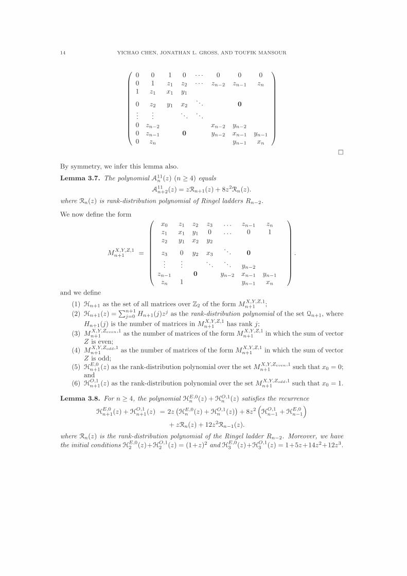
Lemma 3.8. For n ≥ 4, the polynomial HE,0n (z) +HO,1

n (z) satisfies the recurrence

HE,0n+1(z) +H

O,1n+1(z) = 2z

(

HE,0n (z) +H

O,1n (z)

)

+ 8z2(

HO,1n−1 +H

E,0n−1

)

+ zRn(z) + 12z2Rn−1(z).

where Rn(z) is the rank-distribution polynomial of the Ringel ladder Rn−2. Moreover, we have

the initial conditions HE,02 (z)+H

O,12 (z) = (1+z)2 and H

E,03 (z)+H

O,13 (z) = 1+5z+14z2+12z3.


Proof. We first prove the following property:

Claim 1: The polynomial HE,0n (z) (n ≥ 4) satisfies the recurrence

HE,0n+1(z) = z

(

HE,0n (z) +H

O,1n

)

+ zREn (z) + 2z2

(

RO,0n−1(z) + R

E,1n−1

)

+ 2z2(

HE,0n−1(z) +H

O,1n−1

)

+ 4z2(

RE,0n−1(z) +H

E,0n−1

)

+ 2z2Rn−1(z) + 4z2R0n−1(z)


Here the overlap matrix has the following form. The discussion has two cases.

0 z1 z2 z3 . . . zn−1 znz1 x1 y1 0 . . . 0 1z2 y1 x2 y2

z3 0 y2 x3. . . 0

......

. . .. . . yn−2

zn−1 0 yn−2 xn−1 yn−1

zn 1 yn−1 xn

(1) Case 1: xn = 0.• subcase 1: yn−1 = 0, zn = 0. No matter what values z1, x1, and y1 take, wecan transform the matrix above into the following form. Note that there are fourdifferent combinations of values for the variables y1 and x1.

0 0 z2 z3 . . . zn−1 00 0 0 0 . . . 0 1z2 0 x2 y2

z3 0 y2 x3. . . 0

......

. . .. . . yn−2

zn−1 0 yn−2 xn−1 00 1 0 0

When z1 = 0, it contributes a term 4z2RE,0n−1(z). When z1 = 1, it contributes a

term 4z2RO,0n−1(z).

• subcase 2: yn−1 = 0, zn = 1. We add the second row to the first row, and thenadd the second column to the first column. The resulting matrix has the followingform. Note that there are two different possible values for the variable z1.

x1 z1 + x1 z2 + y1 z3 . . . zn−1 0z1 + x1 x1 y1 0 . . . 0 1z2 + y1 y1 x2 y2

z3 0 y2 x3. . . 0

......

. . .. . . yn−2

zn−1 0 yn−2 xn−1 00 1 0 0

When x1 = 0, it contributes a term 2z2R0n−1(z). When x1 = 1, it contributes a

term 2z2R1n−1(z).


• subcase 3: yn−1 = 1, zn = 0. We add row n to the second row, and then addcolumn n to the second column. The resulting matrix has the following form.

0 z1 + zn−1 z2 z3 . . . zn−2 zn−1 0z1 + zn−1 x1 y1 0 . . . yn−2 xn−1 0

z2 y1 x2 y2

z3 0 y2 x3. . . 0

......

. . .. . . yn−3

zn−2 yn−2 yn−3 xn−2 yn−2

zn−1 xn−1 0 yn−2 xn−1 10 0 1 0

No matter what assignments of the variables of zn−1, xn−1, and yn−2, we cantransform the matrix immediately above to the following form. Note that there arefour different choices of the variables zn−1 and xn−1.

0 z1 + zn−1 z2 z3 . . . zn−2 0 0z1 + zn−1 x1 y1 0 . . . yn−2 0 0

z2 y1 x2 y2

z3 0 y2 x3. . . 0

......

. . .. . . yn−3

zn−2 yn−2 yn−3 xn−2 00 0 0 0 0 10 0 1 0

When yn−2 = 0, it contributes a term 4z2RE,0n−1(z). When yn−2 = 1, it contributes

a term 4z2HE,0n−1(z).

• subcase 4: yn−1 = 1, zn = 1. We add row n to the first and second rows, andthen add column n to the first and second columns. The resulting matrix has thefollowing form.

xn−1 z1 + zn−1 + xn−1 z2 z3 . . . zn−2 + yn−2 zn−1 + xn−1 0z1 + zn−1 + xn−1 x1 y1 0 . . . yn−2 xn−1 0

z2 y1 x2 y2

z3 0 y2 x3. . . 0

......

. . .. . . yn−3

zn−2 + yn−2 yn−2 yn−3 xn−2 yn−2

zn−1 + xn−1 xn−1 0 yn−2 xn−1 10 0 1 0


For any combination of values of zn−1, xn−1, and yn−2, we can transform the abovematrix to the following form. Note that there are two possible values for zn−1.

xn−1 z1 + zn−1 + xn−1 z2 z3 . . . zn−2 + yn−2 0 0z1 + zn−1 + xn−1 x1 y1 0 . . . yn−2 0 0

z2 y1 x2 y2

z3 0 y2 x3. . . 0

......

. . .. . . yn−3

zn−2 + yn−2 yn−2 yn−3 xn−2 00 0 0 0 0 10 0 1 0

When yn−2 = 0, depending whether xn−1 = 0 or xn−1 = 1, it contributes 2z2RO,0n−1(z)

or 2z2RE,1n−1(z). When yn−2 = 1, it contributes 2z2HO,0

n−1(z) or 2z2H

E,1n−1(z).

(2) Case 2: xn = 1. There are four subcases.• subcase 1: yn−1 = 0, zn = 0. We add the last row to the second row, and thenadd the last column to the second column. The resulting matrix has the followingform. This subcase contributes zRE,0

n (z).

0 z1 z2 z3 . . . zn−1 0z1 x1 y1 0 . . . 0 0z2 y1 x2 y2

z3 0 y2 x3. . . 0

......

. . .. . . yn−2

zn−1 0 yn−2 xn−1 00 0 0 1

• subcase 2: yn−1 = 0, zn = 1. We add the last row to the first and second rows, andthen add the last column to the first and second columns. The resulting matrixhas the following form. This subcase also contributes a term zRE,1

n (z).

1 z1 + 1 z2 z3 . . . zn−1 0z1 + 1 x1 y1 0 . . . 0 0z2 y1 x2 y2

z3 0 y2 x3. . . 0

......

. . .. . . yn−2

zn−1 0 yn−2 xn−1 00 0 0 1

• subcase 3: yn−1 = 1, zn = 0. We add the last row to rows 2 and n, and then addthe last column to columns 2 and n. The resulting matrix has the following form.


This subcase contributes zHE,0n (z).

0 z1 z2 z3 . . . zn−1 0z1 x1 y1 0 . . . 1 0z2 y1 x2 y2

z3 0 y2 x3. . . 0

......

. . .. . . yn−2

zn−1 1 0 yn−2 xn−1 00 0 0 1

• subcase 4: yn−1 = 1, zn = 1. We add the last row to rows 1, 2, and n, and then addthe last column to the columns 1, 2, and n. The resulting matrix has the followingform. This subcase contributes zHO,1

n (z).

1 z1 + 1 z2 z3 . . . zn−1 + 1 0z1 + 1 x1 y1 0 . . . 1 0z2 y1 x2 y2

z3 0 y2 x3. . . 0

......

. . .. . . yn−2

zn−1 + 1 1 0 yn−2 xn−1 00 0 0 1

In a similar way, we can establish this second claim:

Claim 2: The polynomial HO,1n (z) (n ≥ 4) satisfies the recurrence

HO,1n+1(z) =z

(

HE,0n (z) +H

O,1n

)

+ zROn (z) + 2z2

(

RO,0n−1(z) + R

E,1n−1

)

+ 2z2(

HE,0n−1(z) +H

O,1n−1

)

+ 4z2(

RO,1n−1(z) +H

O,1n−1

)

+ 2z2Rn−1(z) + 4z2R1n−1(z)


The above two claims imply the theorem. �

Proposition 3.9. The generating function H′(t; z) =∑

n≥3(HE,0n (z) +HO,1

n (z))tn is given by

t2f(t; z)

(1− 2t− 4tz − 16z2t2)(1 − t− 4tz − 16z2t2)(1 + 2zt)(1− 4zt),

where

f(t; z) = (1 + z)2 − (2 + 9z2 + 11z − 2z3)t− (1 + 25z2 + 20z4 + 66z3)t2

+ (2− 96z5 + 46z2 + 72z4 + 16z + 136z3)t3 + 16z2(29z2 − 4z4 + 3 + 26z3 + 14z)t4

+ 256z4(1 + z)2t5.

Proof. We multiply the recurrence relation of Lemma 3.8 for the polynomial HE,0n (z)+HO,1

n (z)by tn and we sum over all n ≥ 3 to deduce that the generating function H′(t; z) is given by

t2f(t; z)

(1− 2t− 4tz − 16z2t2)(1 − t− 4tz − 16z2t2)(1 + 2zt)(1− 4zt),

where we used the closed formula of Theorem 3.1 for the generating function R(t; z). �


Lemma 3.10. The polynomial A11n (z) (n ≥ 4) satisfies the equation

A11n+2(z) =2z

(

HE,0n+1(z) +H

O,1n+1

)

+ 8z2(

HE,0n (z) +H

O,1n (z)

)

+ 4z2Rn(z).(6)

where Rn+1(z) is the rank-distribution polynomial of the Ringel ladder Rn−1 and Ln−1(z) is therank-distribution polynomial of the closed-end ladder Ln−2.

Proof. There are two cases.

(1) xe = 1. We add the first row to rows 3 and n + 2, and then add the first column tocolumns 3 and n+ 2. The resulting matrix has the following form.

1 c+ xf 0 0 · · · 0 0 0c+ xf xf z1 + c+ xf z2 · · · zn−2 zn−1 zn + c+ xf

0 z1 + c+ xf x1 y1 1

0 z2 y1 x2. . . 0

......

. . .. . .

0 zn−2 xn−2 yn−2

0 zn−1 0 yn−2 xn−1 yn−1

0 zn + c+ xf 1 yn−1 xn

In the subcase c + xf = 0, we have either c = xf = 0 or c = xf = 1. This subcase

contributes the terms zHE,0n+1(z) and zH

O,1n+1(z). In the subcase c + xf = 1, we have

either c = 0, xf = 1 or c = 1, xf = 0. Here we add the first row to the second row andthen add the first column to the second column. The resulting matrix has the following

form, and this subcase contributes the terms zHE,0n+1(z) and zH

O,1n+1(z).

1 0 0 0 · · · 0 0 00 xf + 1 z1 + 1 z2 · · · zn−2 zn−1 zn + 10 z1 + 1 x1 y1 1

0 z2 y1 x2. . . 0

......

. . .. . .

0 zn−2 xn−2 yn−2

0 zn−1 0 yn−2 xn−1 yn−1

0 zn + 1 1 yn−1 xn

(2) xe = 0. We add the last row to the third row, and then add the last column to the thirdcolumn. The resulting matrix has the following form.

0 c+ xf 0 0 · · · 0 0 1c+ xf xf z1 + zn z2 · · · zn−2 zn−1 zn

0 z1 + zn x1 y1 yn−1 xn

0 z2 y1 x2. . . 0

......

. . .. . .

0 zn−2 xn−2 yn−2

0 zn−1 yn−1 0 yn−2 xn−1 yn−1

1 zn xn yn−1 xn


• subcase 1: c+ xf = 0. No matter what the values of zn, xn and yn−1, the matriximmediately above can be transformed into the following form.

0 0 0 0 · · · 0 0 10 xf z1 + zn z2 · · · zn−2 zn−1 00 z1 + zn x1 y1 yn−1 0

0 z2 y1 x2. . . 0

......

. . .. . .

0 zn−2 xn−2 yn−2

0 zn−1 yn−1 0 yn−2 xn−1 01 0 0 0 0

When yn−1 = 0, according to whether c = xf = 0 or c = xf = 1, this subcasecontributes 4z2RE,0

n (z) or 4z2RO,1n (z). When yn−1 = 1, it contributes 4z2HE,0

n (z)or 4z2HO,1

n (z).• subcase 2: c + xf = 1. We add the last row to the first and second rows, and wethen add the last column to the first and second columns. The resulting matrixhas the following form.

0 0 0 0 · · · 0 0 10 xf z1 + zn + xn z2 · · · zn−2 zn−1 + yn−1 zn + xn

0 z1 + zn + xn x1 y1 yn−1 xn

0 z2 y1 x2. . . 0

......

. . .. . .

0 zn−2 xn−2 yn−2

0 zn−1 + yn−1 yn−1 0 yn−2 xn−1 yn−1

1 zn + xn xn yn−1 xn

For any values of zn, xn and yn−1, the above matrix can be transformed into thefollowing form. When yn−1 = 0, it contributes 2z2Rn(z). When yn−1 = 1, itcontributes 2z2Hn(z).

0 0 0 0 · · · 0 0 10 xf z1 + zn + xn z2 · · · zn−2 zn−1 + yn−1 00 z1 + zn + xn x1 y1 yn−1 0

0 z2 y1 x2. . . 0

......

. . .. . .

0 zn−2 xn−2 yn−2

0 zn−1 + yn−1 yn−1 0 yn−2 xn−1 01 0 0 0 0

�


4. The total embedding polynomial of circular ladders

We recall that the Chebyshev polynomials of the second kind are defined by the Chebyshevrecurrence system:

U0(t) = 1

U1(t) = 2t

Un(t) = 2tUn−1(t)− Un−2(t)(7)

Theorem 4.1. We have∑

n≥4 gCLn(x)tn = 2

tB(t;

√x). Moreover, for all n ≥ 4, the number

of distinct cellular imbeddings of CLn in a surface of genus j is

7n+jj

23j−3(

n−j−1j−1

)

+ n−4j+2j

23j−3(

n−j+1j−1

)

+ nj−12

n+j−1(

n−jj−2

)

+2n−1δn,2j+2 + 2nδn,2j+1 − 3 · 2n−1δn,2j j ≥ 2,2n + 8n− 2 + 8δn,4 j = 1,2 j = 0.

where δ is the Kronecker delta function.

Proof. A derivation of the formula given here is driven by [27]. It is not hard to check that ourformula is equivalent to the original formula of [18, Theorem 3.10]. �

Corollary 4.2. [27] For all n ≥ 4,

gCLn(x) = 1− x+

1− 3x− 2√x

4x(−2

√x)n +

1− 3x+ 2√x

4x(2√x)n

+ 2nx(i√2x)n

[

Un

(

1

2i√2x

)

− Un−2

(

1

2i√2x

)]

+ (1 − x)(2i√2x)n

[

Un

(

1

4i√2x

)

− Un−2

(

1

4i√2x

)]

,

where Us is the sth Chebyshev polynomial of the second kind and i2 = −1

Now we can prove our main result.

Theorem 4.3. The generating function A(t; z) =∑

n≥2 An(z)tn is given by

t2f(t; z)

(1− 2t− 4tz − 16z2t2)(1− t− 4tz − 16z2t2)(1− t− 2tz)(1 + 2tz)(1− 4tz),

where

f(t; z) = (1 + z)2 + 2(z − 1)(6z2 + 6z + 1)t− (67z2 + 9z + 162z3 + 2 + 68z4)t2

+ (141z2 + 282z3 + 5 + 8z4 + 44z − 384z5)t3

+ (1424z4 + 2z2 − 2 + 704z6 + 424z3 + 2128z5 − 24z)t4

+ 32z2(6z + 1)(16z4 + 7z3 − 5z2 − 6z − 2)t5 − 128z4(5 + 58z3 + 32z + 69z2)t6

− 2048z6(1 + 2z)(1 + z)2t7.


Proof. By Property 2.8, Lemmas 3.5, 3.6, 3.7, and 3.10 together with Lemmas 3.3 and 3.8 weobtain

An(z) = RE,0n (z) + R

O,1n (z) +H

E,0n (z) +H

O,1n (z).

By multiplying by tn and summing over all n ≥ 2, we have

A(t; z) = H′(t; z) + R

′(t; z),

where the generating functions H′(t; z) and R′(t; z) are given by Propositions 3.4 and 3.9, re-spectively. �

Theorem 4.4. For all n ≥ 4, the total genus polynomial of circular ladders CLn is as follows:

ICLn(x, y) = 2Bn+1(

√x) + 2An+1(y)− 2Bn+1(y).

The generating function ICL(t;x, y) =∑

n≥3 ICLn(x, y)tn is given by

ICL(t;x, y) =2

t

(

B(t;√x) +A(t; y)− (1 + y)2t2 − (2 + 24y3 + 10y + 28y2)t3

− (1 + 11y + 80y2 + 212y3 + 208y4)t4 −B(t; y)

)

.

Moreover, for all n ≥ 4,

ICLn(x, y) = y2 − x+

1− 3x− 2√x

4x(−2

√x)n +

1− 3x+ 2√x

4x(2√x)n

+ x(2i√2x)nβn

(

1

2i√2x

)

+ (1− x)(2i√2x)nβn

(

1

4i√2x

)

− (y2 − 1)(6y + 1)(4y)n−1

3y− (4y − 1)(3y − 1)(y + 1)(−2y)n−2

3+ (1− y)(1 + 2y)n

+ (3y + 1)(y − 1)(2y)n−2 + 2(y2 − 1)(2√2iy)nαn

(

1

4√2iy

)

− 2y2(2√2iy)nαn

(

1

2√2iy

)

+ 2(1− y)(1 + 2y)(4iy)nαn

(

1 + 4y

8iy

)

+ 4y2(4iy)nαn

(

1 + 2y

4iy

)

where Us is the s-th Chebyshev polynomial of the second kind, i2 = −1,

αn(t) = Un(t)− tUn−1(t) and βn(t) = Un(t)− Un−2(t).

Proof. By Property 2.7, we have ICLn(x, y) = 2Bn+1(

√x)+ 2An+1(y)− 2Bn+1(y). Multiplying

by tn and summing over all n ≥ 4 with using Theorems 4.1 and 4.3, we obtain

ICL(t;x, y) =2

t

(

B(t;√x) +A(t; y)− (1 + y)2t2 − (2 + 24y3 + 10y + 28y2)t3

− (1 + 11y + 80y2 + 212y3 + 208y4)t4 −B(t; y)

)

.


Clearly, the coefficient of tn, n ≥ 4, in 2tB(t;

√x) is given by Corollary 4.2. Now we consider

the coefficient of tn in

f =2

t

(

A(t; y)− (1 + y)2t2 − (2 + 24y3 + 10y + 28y2)t3

− (1 + 11y + 80y2 + 212y3 + 208y4)t4 −B(t; y)

)

.

Rewriting f by partial fraction decomposition, we obtain

f = −2(196y3 + 212y2 + 61y + 11)yt3 − 4(12y2 + 11y + 5)yt2 − 4(y + 2)yt− y2

− y2 − 2y3 + 2y − 1

4y2+

y2 − 1

1− t+

1 + 6y − 6y3 − y2

12y2(1− 4ty)+

3y2 − 2y − 1

4y2(1− 2ty)− 12y3 + 5y2 − 6y + 1

12y2(1 + 2ty)

+1− y

1− t− 2ty+

2y2 − 2− y2t+ t

1− t− 8y2t2− 2y2(1− t)

1− 2t− 8y2t2+

2 + 2y − 4y2 + 8y3t− t− 2y2t− 5ty

1− t− 4ty − 16y2t2

+4y2(1− t− 2ty)

1− 2t− 4ty − 16y2t2.

Let n ≥ 4, then the coefficient of tn in f is given by

[tn]f = [tn]

{

y2 − 1

1− t+

1 + 6y − 6y3 − y2

12y2(1− 4ty)+

3y2 − 2y − 1

4y2(1− 2ty)− 12y3 + 5y2 − 6y + 1

12y2(1 + 2ty)

+1− y

1− t− 2ty+

2y2 − 2− y2t+ t

1− t− 8y2t2− 2y2(1− t)

1− 2t− 8y2t2

+2 + 2y − 4y2 + 8y3t− t− 2y2t− 5ty

1− t− 4ty − 16y2t2+

4y2(1− t− 2ty)

1− 2t− 4ty − 16y2t2.

}

,

which is equivalent to

[tn]f = y2 − 1− (y2 − 1)(6y + 1)(4y)n−1

3y− (4y − 1)(3y − 1)(y + 1)(−2y)n−2

3+ (1 − y)(1 + 2y)n

+ (3y + 1)(y − 1)(2y)n−2 + 2(y2 − 1)(2√2iy)nαn

(

1

4√2iy

)

− 2y2(2√2iy)nαn

(

1

2√2iy

)

+ 2(1− y)(1 + 2y)(4iy)nαn

(

1 + 4y

8iy

)

+ 4y2(4iy)nαn

(

1 + 2y

4iy

)

,

which completes the proof. �

For instance our theorem for n = 4, 5, 6, 7 gives

ICL4(x, y) = 2 + 54x+ 24y + 200x2 + 1288y3 + 3264y4 + 192y2 + 3168y5

ICL5(x, y) = 2 + 70x+ 30y + 320x3 + 632x2 + 2560y3 + 11240y4 + 23232y6 + 282y2 + 27168y5

ICL6(x, y) = 2 + 110x+ 36y + 2656x3 + 1328x2 + 4740y3 + 27360y4 + 169856y7 + 211840y6

+ 424y2 + 105936y5

ICL7(x, y) = 2 + 182x+ 42y + 3584x4 + 9984x3 + 2632x2 + 8652y3 + 60368y4 + 1663488y7

+ 933408y6 + 618y2 + 1208832y8 + 302512y5


References

[1] D. Archdeacon, Calculations on the average genus and genus distribution of graphs, Congr. Numer. 67

(1988) 114–124.[2] J. Chen, J. L. Gross, and R. G. Rieper, Overlap matrices and total embeddings, Discrete Math. 128 (1994)

73–94.[3] Y. Chen, T. Mansour, and Q. Zou, Embedding distributions and Chebyshev polynomial, Graphs and Com-

bin., Online 22 August 2011, in press. DOI 10.1007/s00373-011-1075-5[4] Y. Chen, L. Ou, and Q. Zou, Total embedding distributions of Ringel ladders, Discrete Math. 311 (2011)

2463–2474.[5] Y. Chen, J. L. Gross, and T. Mansour, Genus distributions of star-ladders, Discrete Math. To appear.[6] M. Furst, J. Gross, and R. Statman, Genus distributions for two classes of graphs, J. Combin. Ser. B 46

(1989) 22–36.[7] J. L. Gross and M. L. Furst, Hierarchy for imbedding-distribution invariants of a graph, J. Graph Theory

11 (1987) 205–220.[8] J. L. Gross, D. P. Robbins and T. W. Tucker, Genus distributions for bouquets of circles, J. Combin. Theory

(B) 47 (1989) 292–306.[9] J. L. Gross and T. W. Tucker, Topological Graph Theory, Dover, 2001; (original edn. Wiley, 1987).

[10] J. L. Gross, Genus distribution of graphs under surgery: adding edges and splitting vertices. New York J.

Math. 16 (2010) 161–178.[11] J. L. Gross, Genus distributions of cubic outerplanar graphs, J. Graph Algorithms and Applications 15(2)

(2011) 295–316.[12] J. L. Gross, Embeddings of graphs of fixed treewidth and bounded degree, Abstract 1077-05-1655, Boston

Meeting of the Amer. Math. Soc. (Jan. 2012).[13] W. Gustin, Orientable embedding of Cayley graphs, Bull. Amer. Math. Soc. 69 (1963) 272–275.[14] I. F. Khan, M. I. Poshni, and J. L. Gross, Genus distribution of graph amalgamations: pasting when one

root has higher degree, Ars Math. Contemp. 3 (2010) 121–138.[15] J. H. Kwak and S. H. Shim, Total embedding distributions for bouquets of circles, Discrete Math. 248 (2002)

93–108.[16] D. Li, Genus distribution for circular ladders, Northeastern Mathematics Journal 16 (2)(2000) 181–189[17] D. Li, Genus distributions of Mobius ladders, Northeastern Mathematics Journal 21 (1)(2005) 70–80.[18] L. A. McGeoch, Genus distribution for circular and Mobius ladders, Technical report extracted from PhD

thesis, Carnegie-Mellon University, 1987.[19] B. Mohar, An obstruction to embedding graphs in surfaces, Discrete Math. 78 (1989) 135–142.[20] M. I. Poshni, I. F. Khan, and J. L. Gross, Genus distribution of edge-amalgamations, Ars Math. Contemp.

3 (2010) 69–86.[21] S. Stahl, Region distributions of graph embeddings and Stirling numbers, Discrete Math. 82 (1990) 57–78.[22] S. Stahl, Permutation-partition pairs III: Embedding distributions of linear families of graphs, J. Combin.

Theory (B) 52 (1991) 191–218.[23] S. Stahl, Region distributions of some small diameter graphs, Discrete Math. 89 (1991) 281–299.[24] G. Ringel, Map Color Theorem, Springer-Verlag, 1974.[25] L. X. Wan and Y. P. Liu, Orientable embedding genus distribution for certain types of graphs, J. Combin.

Theory (B) 47 (2008) 19–32.[26] Y. Yang and Y. Liu, Number of embeddings of circular and Mobius ladders on surfaces, Science China

Mathematics 53 (5) (2010) 1393–1405.[27] http://www.cs.columbia.edu/∼gross/

College of Mathematics and Econometrics, Hunan University, 410082 Changsha, China

E-mail address: [email protected]

Department of Computer Science, Columbia University, New York, NY 10027 USA


Department of Mathematics, University of Haifa, 31905 Haifa, Israel


Documents

Introduction - cs.columbia.edu