Introduction Economics Lecture 1c - Yolabalasubramanian.yolasite.com/resources/Introduction Economics Le… · Introduction Economics Lecture 1c.pptx Author: BALASUBRAMANIAN SIVASWAMY

Department of Chemical Engineering SRM University

CH0401 Process Engineering Economics

Lecture 1c

Balasubramanian S

Balasubramanian S Department of Chemical Engineering 2

Process Engineering Economics

1

2

3

4

5

Introduction – Time Value of Money

Equivalence

Equations for economic studies

Amortization

Depreciation and Depletion



1

2

3

4

5


Equivalence


Amortization




1

2

3

4

5


Equivalence


Amortization



Process Engineering Economics – Equations for economic studies

S.No Equation Use

1. F = P(1+ i)n = PCF Single payment at the end of nth period

2. R = P i(1+ i)n

(1+ i)n !1"#$

%&'= PPF

Uniform payment at the end of period (to pay fixed amount each year)

3. F = R (1+ i)n !1i

"#$

%&'

Future worth at the end of nth period

4. P = R (1+ i)n !1i(1+ i)n

"#$

%&'= RPF Present Worth

!


S.No Equation Use 4.

P = R (1+ i)n !1i(1+ i)n

"#$

%&'= RPF

Present Worth

5. R = (P ! L) i(1+ i)n

(1+ i)n !1"#$

%&'+ L ( i

Uniform payment with salvage (L)

6. (1+ i)n = 1

1! PR

"#$

%&' i

Rate of return or payment time when L is zero or salvage is neglected

7.

n =! log 1! i P

R"#$

%&'

log(1+ i)

Payment time when L is zero or salvage is neglected

!



S. No Equation Use 8.

P ' = R 'i '

Capitalized costs (or) perpetual uniform payment R! to an equivalent capital cost P! at he present time for a given interest rate.

9. Ck = (CFC ! SFD ) fk

! fk =(1+ i)n

(1+ i)n !1

Capitalized cost including cost factor.

10. R '' = P i '

(1+ i ')n !1"#$

%&'

Sinking fund deposit, i" – is sinking fund interest rate and L is zero.

11. P = R ''' (1+ i ')n !1

i (1+ i ')n !1"# $% + i '

&

'(

)

*+

Hoskold’s formula - is rate of return, i! is sinking fund interest rate. Note that when i = i! equation (10) reduces to equation (4)

!



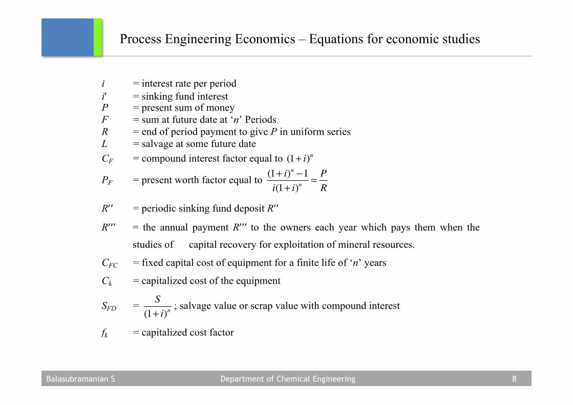
i = interest rate per period i! = sinking fund interest P = present sum of money F = sum at future date at ‘n’ Periods R = end of period payment to give P in uniform series L = salvage at some future date CF = compound interest factor equal to (1+ i)n

PF = present worth factor equal to (1+ i)n !1i(1+ i)n

= PR

R"" = periodic sinking fund deposit R""

R""" = the annual payment R"""# to the owners each year which pays them when the

studies of capital recovery for exploitation of mineral resources.

CFC = fixed capital cost of equipment for a finite life of ‘n’ years

Ck = capitalized cost of the equipment

SFD = S

(1+ i)n; salvage value or scrap value with compound interest

fk = capitalized cost factor

!



In the above table i.e. equations used for economic studies, the compound interest factors

used in all the equations from 1 to ll are based on two series

•  Single Payment series

•  Uniform annual series




Interest formulas relating a uniform series to its present worth and future worth

We will use the relationship F = P(1+i)n in our uniform series derivation

The general relationship between R and F is shown in the figure given below

Where R = An end of period uniform series for n periods F = Future sum or Future worth



Looking at the figure given below we see that if amount R is invested at end of each

year for 4 years, the total amount F at the end of 4 years will be the sum of the

compound amounts of the individual investments

Where R = An end of period uniform series for n periods F = Future sum or Future worth

In general case for n years



Multiplying equation (1) by (1+i), we have

Factoring out R and subtracting equation (1) gives

Solving above equation for F gives iF = R[(1+ i)n !1]

F= R (1+ i)n !1i

"

#$

%

&' ! ! ! !(5)



Thus we have an equation for F when R known i.e

The term inside the brackets

(1+ i)n !1i

"

#$

%

&' is called uniform series

compound amount factor

F= R (1+ i)n !1i

"

#$

%

&' ! ! ! !(5)



We know that

F= R (1+ i)n !1i

"

#$

%

&' ! ! ! !(5)

F= P(1+ i)n Substituting this equation for F in equation (5) we get

P(1+ i)n= R (1+ i)n !1i

"

#$

%

&'

P = R (1+ i)n !1i(1+ i)n

"

#$

%

&' ! ! ! !(6)

Above equation (6) takes the form of equation no. 4 of equations for economic studies

given in the table (slide no. 6). The equation (6) can be used to calculate P if R is

known. (Nomenclature for the above equations are given in slide no. 8)



F= R (1+ i)n !1i

"

#$

%

&' ! ! ! !(5)

P = R (1+ i)n !1i(1+ i)n

"

#$

%

&' ! ! ! !(6)


given in the table (slide no. 5). The equation (5) can be used to calculate F if R is


We know that

Rearranging the above equation (6), we have

PR= (1+ i)n !1

i(1+ i)n"

#$

%

&'

R = P i(1+ i)n

(1+ i)n !1"

#$

%

&' ---- (7)



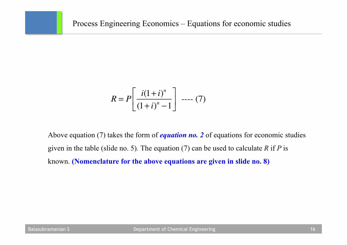
R = P i(1+ i)n

(1+ i)n !1"

#$

%

&' ---- (7)


given in the table (slide no. 5). The equation (7) can be used to calculate R if P is




Above equation (7) or equation no. 2 of equations for economic studies given in the

table (slide no. 5) can be re arranged as follows .

R = P i(1+ i)n

(1+ i)n !1"

#$

%

&' ---- (7)

R[(1+ i)n !1] = Pi(1+ i)n

[(1+ i)n !1] = PiR

[(1+ i)n ]

[(1+ i)n !1](1+ i)n

= PiR

(1+ i)n

(1+ i)n! 1

(1+ i)n= PiR



1= PiR

1= PiR+ 1

(1+ i)n

1! PiR

= 1(1+ i)n

1! PiR

= 1(1+ i)n

1

1! PiR

= (1+ i)n

i.e. (1+ i)n = 1

1! PiR

-----(8)



(1+ i)n = 1

1! PiR

-----(8)


given in the table (slide no. 6). The equation (8) can be used to calculate rate of return

or Payment time when L is zero or salvage/scrap value is neglected. (Nomenclature

for the above equations are given in slide no. 8)

Taking log on both sides of equation (8) we have

n log(1+ i) = log(1)! log 1! PiR

"#$

%&'

n =! log 1! Pi

R"#$

%&'

log(1+ i) ----- (9)




given in the table (slide no. 6). The equation (8) can be used to calculate rate of return

or Payment time when L is zero or salvage/scrap value is neglected. (Nomenclature

for the above equations are given in slide no. 8)

n log(1+ i) = log(1)! log 1! PiR

"#$

%&'

n =! log 1! Pi

R"#$

%&'

log(1+ i) ----- (9)


Process Engineering Economics – References

•  Herbert E. Schweyer. (1955) Process Engineering Economics, Mc Graw Hill •  Max S. Peters, Kaus D. Timmerhaus, Ronald E. West. (2004) Plant

Design and Economics for Chemical Engineers, 5th Ed., Mc Graw Hill

•  Max Kurtz. (1920) Engineering Economics for Professional Engineers’ Examinations, 3rd Ed., Mc Graw Hill

•  Frederic C. Jelen, James H. Black. (1985) Cost and Optimization Engineering, International Student edition, Mc Graw Hill

•  Grant L. E, Grant Ireson. W, Leavenworth S. R. (1982) Principles of Engineering Economy, 7th Ed., John Wiley and Sons.

Documents

Introduction Economics Lecture 1c - Yolabalasubramanian.yolasite.com/resources/Introduction Economics Le… · Introduction Economics Lecture 1c.pptx Author: BALASUBRAMANIAN SIVASWAMY