Embed Size (px)
Citation preview
Introduction
FSNLP, chapter 1
Christopher Manning andHinrich Schütze
© 1999–2002
1
NLP: An Age of Engineering
• 70s/80s: Science of the mind
– Big questions of cognition
– Small simulations (SHRDLU, LUNAR, . . . )
• 1990s: Real problems; rigorous evaluation
– Big corpora on big hard disks
– Applications: web, speech, (vertical)
– Greatly favors statistical techniques
• 2000s: The future is meaning?
2
What is statistical NLP?
• P(to|Sarah drove)
• P(time is a verb|S = Time flies like an arrow)
• P(NP→ Det Adj N|Mother = VP[drive])
• Statistical NLP methods:
– Involve deriving numerical data from text
– Are usually but not always probabilistic (broad
church – we include e.g., vector spaces)
3
StatNLP: Relation to wider context
• Matches move from logic-based AI to probabilistic AI
– Knowledge→ probability distributions
– Inference→ conditional distributions
• Probabilities give opportunity to unify reasoning, plan-
ning, and learning, with communication
• There is now widespread use of machine learning (ML)
methods in NLP (perhaps even overuse?)
• Use of approximation for hard problems
4
Questions that linguistics should answer
• What kinds of things do people say?
• What do these things say/ask/request about the world?
Example: In addition to this, she insisted that women were
regarded as a different existence from men unfairly.
• Text corpora give us data with which to answer these
questions
• They are an externalization of linguistic knowledge
• What words, rules, statistical facts do we find?
• Can we build programs that learn effectively from this
data, and can then do NLP tasks?
5
The big questions for linguistics/NLP
• What kinds of things do people say?
• What do these things say/ask/request about
the world?
These involve questions of frequency, probability,
and likelihood
“Statistical considerations are essential to an un-
derstanding of the operation and development of
languages” – Lyons (1968: 98)
6
Probabilistic grammars in linguistics
• The predictions about grammaticality and ambiguity of
categorical grammars do not accord with human per-
ceptions or engineering needs
• Categorical grammars aren’t predictive
– They don’t tell us what “sounds natural”
– Grammatical but unnatural e.g.: In addition to this,
she insisted that women were regarded as a differ-
ent existence from men unfairly.
7
Big picture claims
• Human cognition has a probabilistic nature
• We are continually faced with uncertain and incomplete
information, and have to reason and interpret as best
we can with the information available
• Language understanding is a case of this
• Language understanding involves mapping from ideas
expressed in a symbol system to an uncertain and in-
complete understanding
Symbol system↔ Probabilistic cognition
8
All parts of natural language text are ambigu-ous
• Real language is highly ambiguous at all levels
• It is thus hard to process
• Humans mostly do not notice the high level of ambiguity
because they resolve ambiguities in real time, by in-
corporating diverse sources of evidence, including fre-
quency information (cf. recent psycholinguistic litera-
ture)
• Goal of computational linguistics is to do as well
• Use of probabilities allows effective evidence combina-
tion within NLP models
9
Contextuality of language
• Language use is situated
• People say the little that is needed to be understood in
a certain situation
• Consequently
– language is highly ambiguous
– tasks like translation involve (probabilistically) recon-
structing world knowledge not in the source text
• We also need to explore quantitative techniques to move
away from the unrealistic categorical assumptions of
much of formal linguistics
10
Computer NLP
• Is often serial through a pipeline (not parallel)
• All components resolve ambiguities
• Something like an n-best list or word lattice is used to
allow some decisions to be deferred until later
• Progressively richer probabilistic models can filter less
likely word sequences, syntactic structures, meanings,
etc.
11
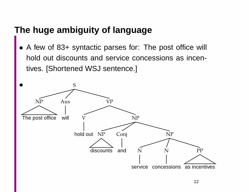
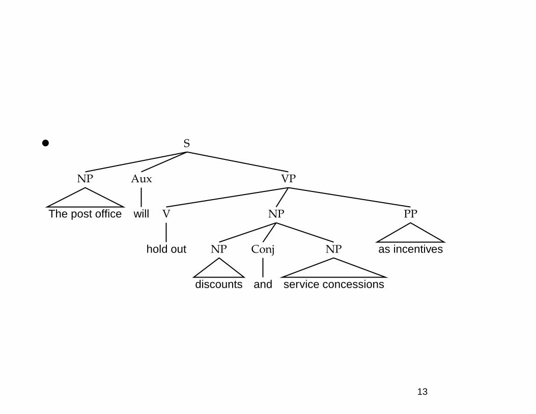
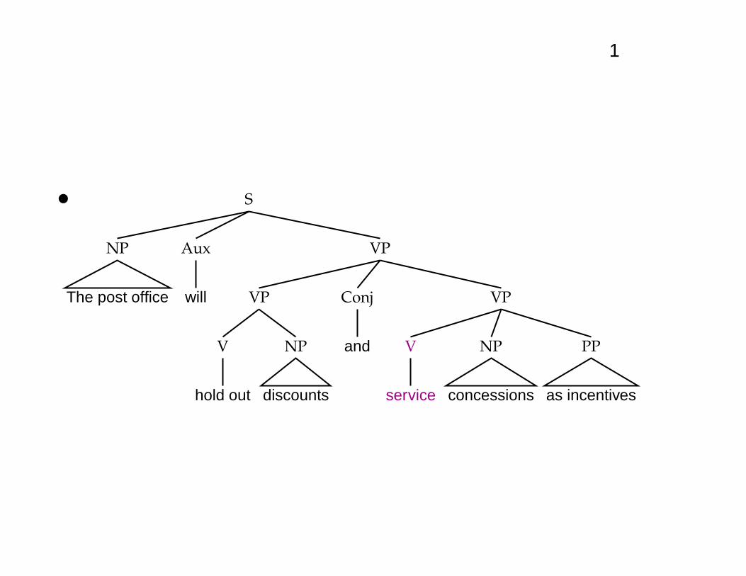
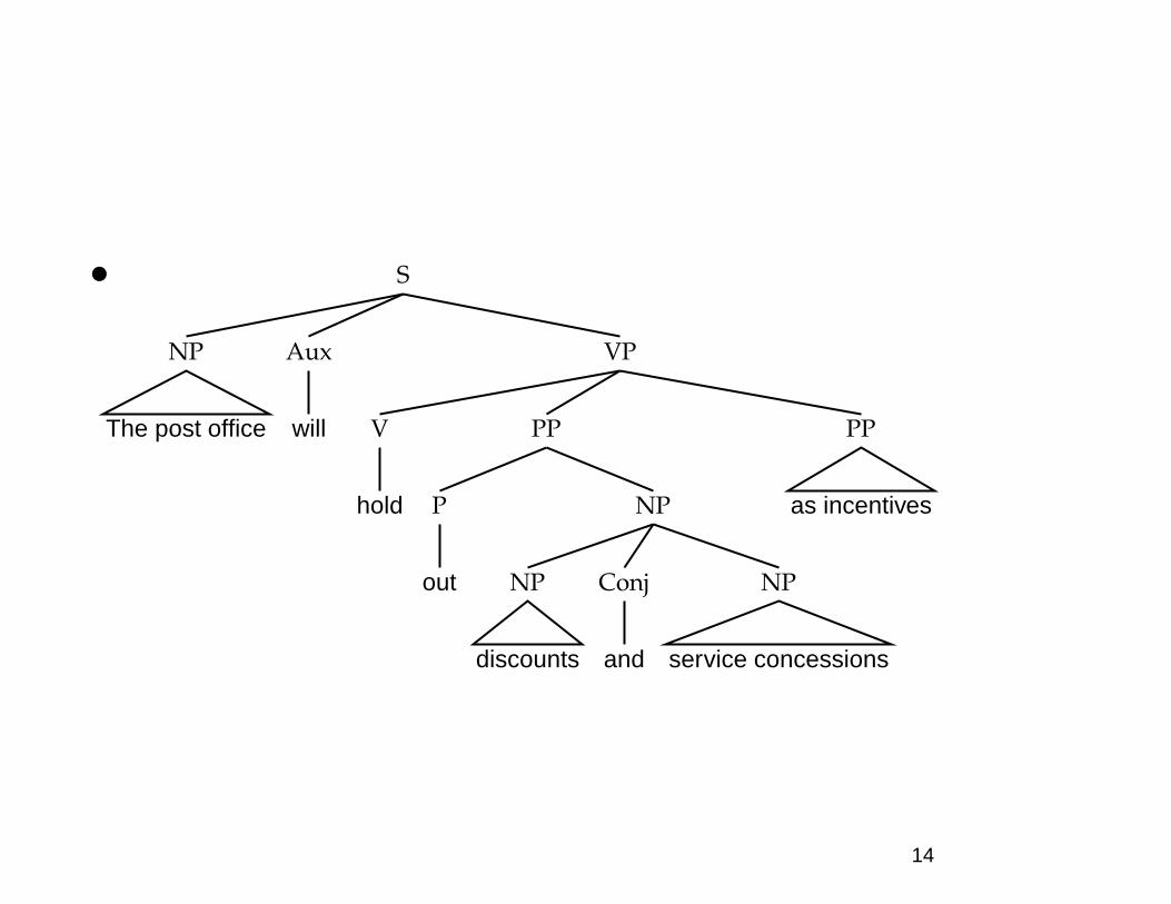
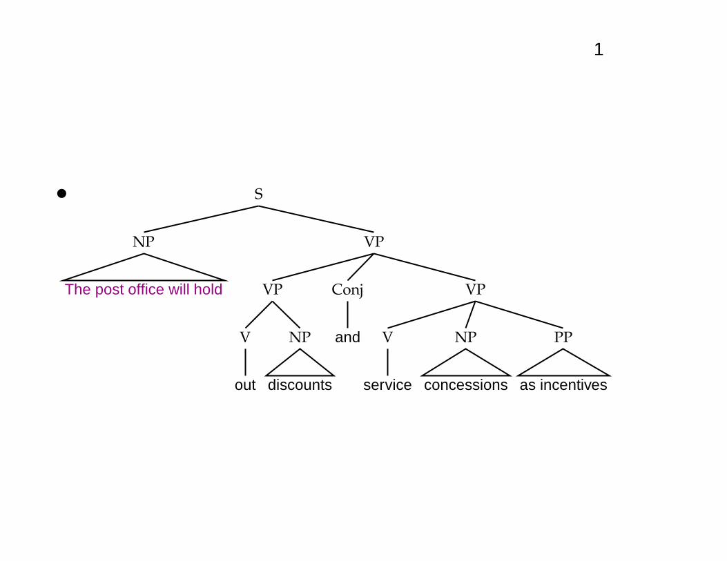
The huge ambiguity of language
• A few of 83+ syntactic parses for: The post office willhold out discounts and service concessions as incen-tives. [Shortened WSJ sentence.]
• S
NP
The post office
Aux
will
VP
V
hold out
NP
NP
discounts
Conj
and
NP
N
service
N
concessions
PP
as incentives
12
• S
NP
The post office
Aux
will
VP
V
hold out
NP
NP
discounts
Conj
and
NP
service concessions
PP
as incentives
13
1
• S
NP
The post office
Aux
will
VP
VP
V
hold out
NP
discounts
Conj
and
VP
V
service
NP
concessions
PP
as incentives
• S
NP
The post office
Aux
will
VP
V
hold
PP
P
out
NP
NP
discounts
Conj
and
NP
service concessions
PP
as incentives
14
1
• S
NP
The post office will hold
VP
VP
V
out
NP
discounts
Conj
and
VP
V
service
NP
concessions
PP
as incentives
Where do problems come in?
Syntax
• Part of speech ambiguities
• Attachment ambiguities
Semantics
• Word sense ambiguities → we’ll start here
• (Semantic interpretation and scope ambigui-
ties)
15
How do we solve them?
Hand-crafted NLP systems
• Easy to encode linguistic knowledge precisely
• Readily comprehensible rules
• Construction is costly
• Feature interactions are hard to manage
• Systems are usually nonprobabilistic
16
Statistical Computational Methods
• Many techniques are used:
– n-grams, history-based models, decision trees / de-
cision lists, memory-based learning, loglinear mod-
els, HMMs, neural networks, vector spaces, graphi-
cal models, PCFGs, . . .
• Robust
• Good for learning (well, supervised learning works well;
unsupervised learning is still hard)
• More work needed on encoding subtle linguistic phe-
nomena
17

Distinctiveness of NLP as an ML problem
• Language allows the complex compositional encoding
of thoughts, ideas, feelings, . . . , intelligence.
• We are minimally dealing with hierarchical structures
(branching processes), and often want to allow more
complex forms of information sharing (dependencies).
• Enormous problems with data sparseness
• Both features and assigned classes regularly involve
multinomial distributions over huge numbers of values
(often in the tens of thousands)
• Generally dealing with discrete distributions though!
• The distributions are very uneven, and have fat tails
18

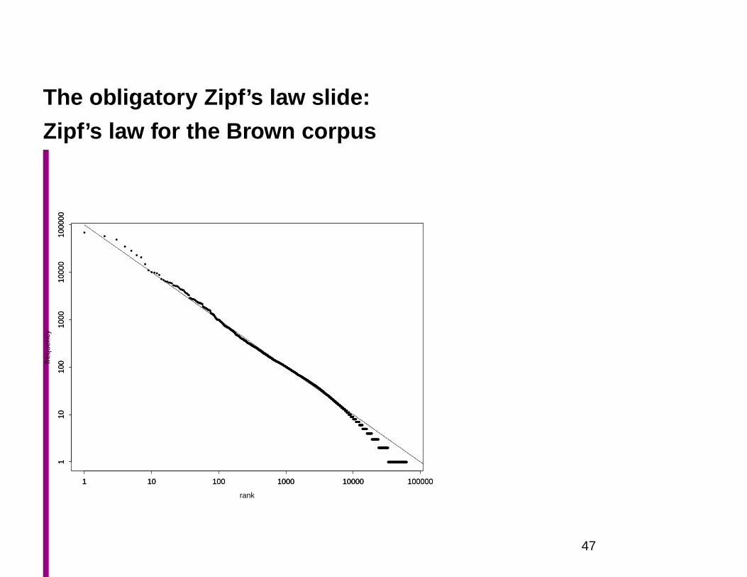
The obligatory Zipf’s law slide:
Zipf’s law for the Brown corpus
• • •• •
• •••••••••••••••••••••••••••••••••••••••••••••••••••••••••••••••••••••••••••••••••••••••••••••••••••••••••••••••••••••••••••••••••••••••••••••••••••••••••••••••••••••••••••••••••••••••••••••••••••••••••••••••••••••••••••••••••••••••••••••••••••••••••••••••••••••••••••••••••••••••••••••••••••••••••••••••••••••••••••••••••••••••••••••••••••••••••••••••••••••••••••••••••••••••••••••••••••••••••••••••••••••••••••••••••••••••••••••••••••••••••••••••••••••••••••••••••••••••••••••••••••••••••••••••••••••••••••••••••••••••••••••••••••••••••••••••••••••••••••••••••••••••••••••••••••••••••••••••••••••••••••••••••••••••••••••••••••••••••••••••••••••••••••••••••••••••••••••••••••••••••••••••••••••••••••••••••••••••••••••••••••••••••••••••••••••••••••••••••••••••••••••••••••••••••••••••••••••••••••••••••••••••••••••••••••••••••••••••••••••••••••••••••••••••••••••••••••••••••••••••••••••••••••••••••••••••••••••••••••••••••••••••••••••••••••••••••••••••••••••••••••••••••••••••••••••••••••••••••••••••••••••••••••••••••••••••••••••••••••••••••••••••••••••••••••••••••••••••••••••••••••••••••••••••••••••••••••••••••••••••••••••••••••••••••••••••••••••••••••••••••••••••••••••••••••••••••••••••••••••••••••••••••••••••••••••••••••••••••••••••••••••••••••••••••••••••••••••••••••••••••••••••••••••••••••••••••••••••••••••••••••••••••••••••••••••••••••••
•••••••••••••••••••••••••••••••••••••••••••••••••••••••••••••••••••••••••••••••••••••••••••
••••••••••••••••••••••••••••••••••••••••••••••••••••••••••••••••••••••••••
•••••••••••••••••••••••••••••••••••••••••••••••••••••••••••••••••••••••••••••••••••••••••••••••••••••••••••••••••••••••••••••••••••••••••••••••
rank
freq
uenc
y
1 10 100 1000 10000 100000
110
100
1000
1000
010
0000
1 10 100 1000 10000 100000
110
100
1000
1000
010
0000
19

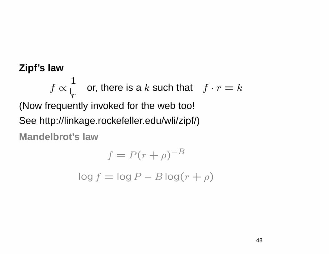
Zipf’s law
f ∝ 1
ror, there is a k such that f · r = k
(Now frequently invoked for the web too!
See http://linkage.rockefeller.edu/wli/zipf/)
Mandelbrot’s law
f = P (r+ ρ)−B
log f = logP −B log(r+ ρ)
20
Corpora
• A corpus is a body of naturally occurring text, normally
one organized or selected in some way
– Latin: one corpus, two corpora
• A balanced corpus tries to be representative across a
language or other domain
• Balance is something of a chimaera: What is balanced?
Who spends what percent of their time reading the sports
pages?
21
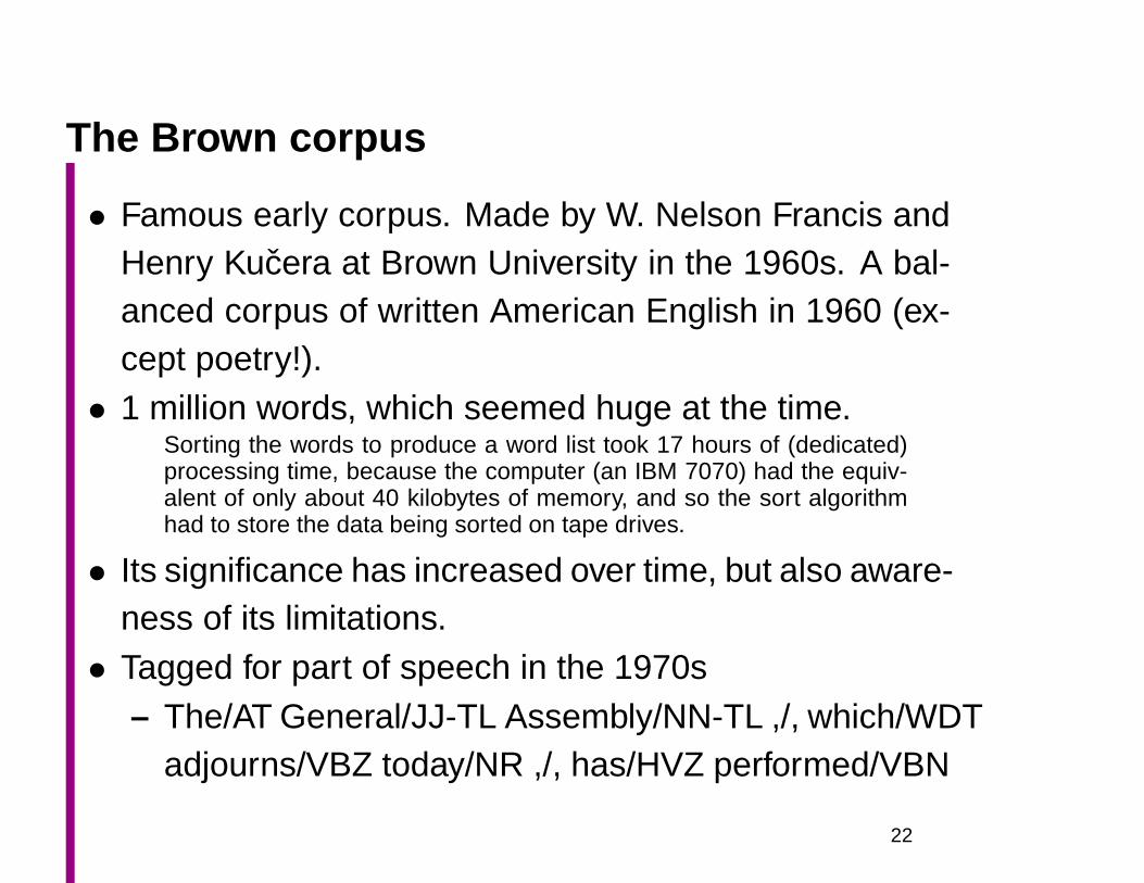
The Brown corpus
• Famous early corpus. Made by W. Nelson Francis andHenry Kucera at Brown University in the 1960s. A bal-anced corpus of written American English in 1960 (ex-cept poetry!).• 1 million words, which seemed huge at the time.
Sorting the words to produce a word list took 17 hours of (dedicated)processing time, because the computer (an IBM 7070) had the equiv-alent of only about 40 kilobytes of memory, and so the sort algorithmhad to store the data being sorted on tape drives.
• Its significance has increased over time, but also aware-ness of its limitations.• Tagged for part of speech in the 1970s
– The/AT General/JJ-TL Assembly/NN-TL ,/, which/WDTadjourns/VBZ today/NR ,/, has/HVZ performed/VBN
22
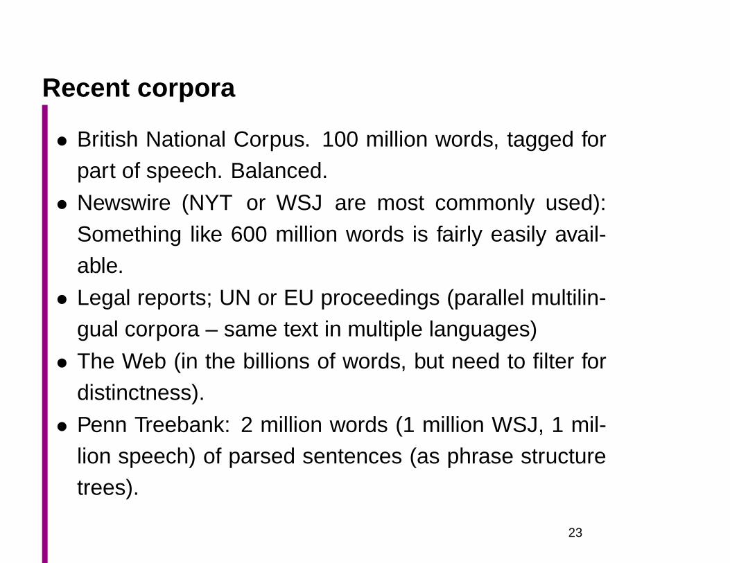
Recent corpora
• British National Corpus. 100 million words, tagged forpart of speech. Balanced.
• Newswire (NYT or WSJ are most commonly used):Something like 600 million words is fairly easily avail-able.
• Legal reports; UN or EU proceedings (parallel multilin-gual corpora – same text in multiple languages)
• The Web (in the billions of words, but need to filter fordistinctness).
• Penn Treebank: 2 million words (1 million WSJ, 1 mil-lion speech) of parsed sentences (as phrase structuretrees).
23
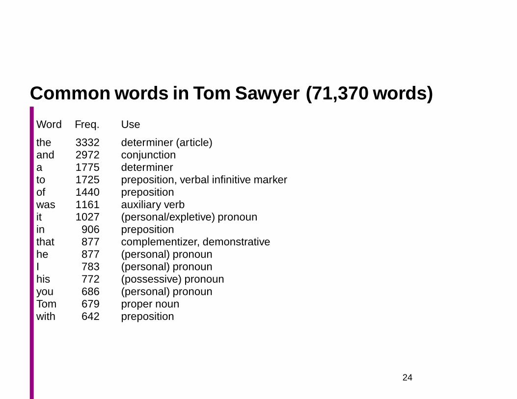
Common words in Tom Sawyer (71,370 words)
Word Freq. Use
the 3332 determiner (article)and 2972 conjunctiona 1775 determinerto 1725 preposition, verbal infinitive markerof 1440 prepositionwas 1161 auxiliary verbit 1027 (personal/expletive) pronounin 906 prepositionthat 877 complementizer, demonstrativehe 877 (personal) pronounI 783 (personal) pronounhis 772 (possessive) pronounyou 686 (personal) pronounTom 679 proper nounwith 642 preposition
24
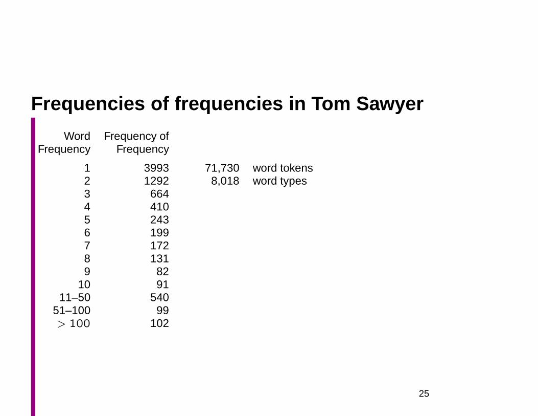
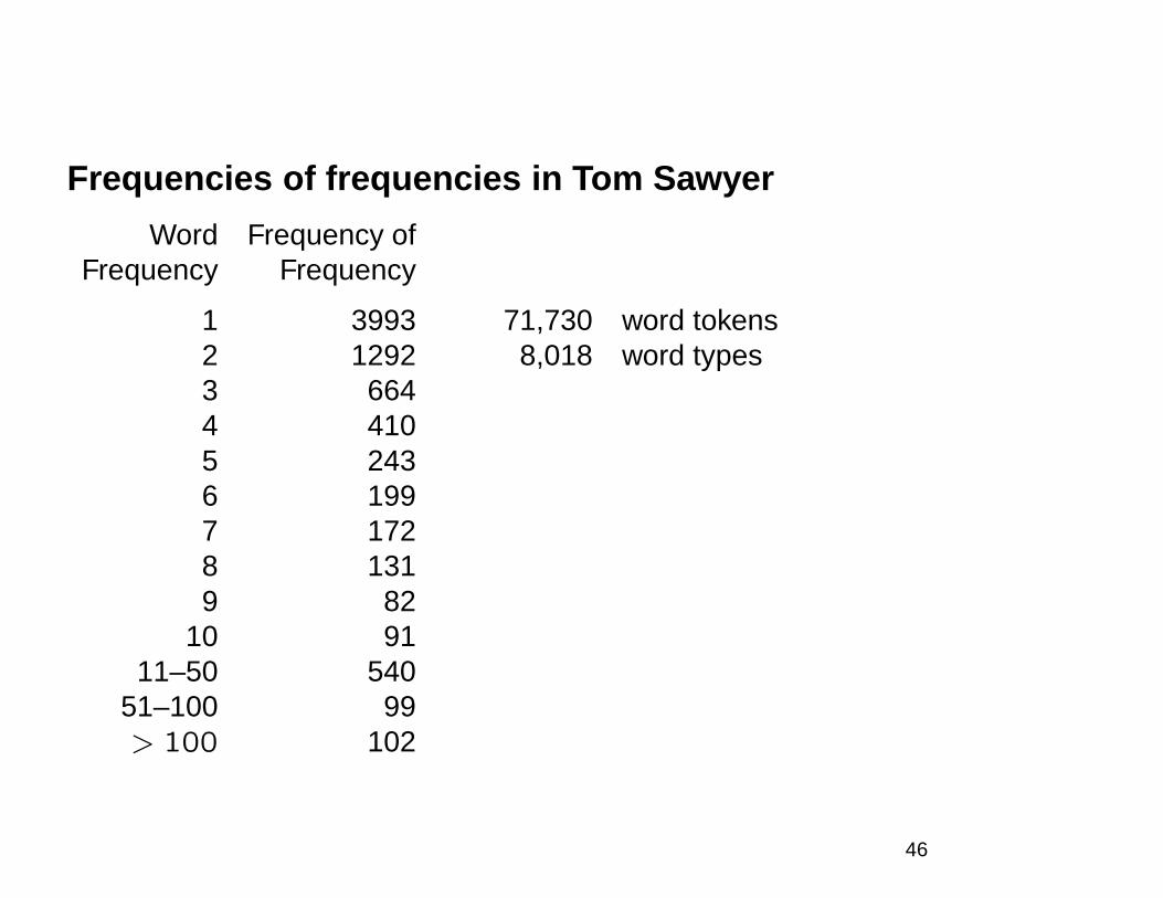
Frequencies of frequencies in Tom Sawyer
Word Frequency ofFrequency Frequency
1 3993 71,730 word tokens2 1292 8,018 word types3 6644 4105 2436 1997 1728 1319 82
10 9111–50 540
51–100 99> 100 102
25
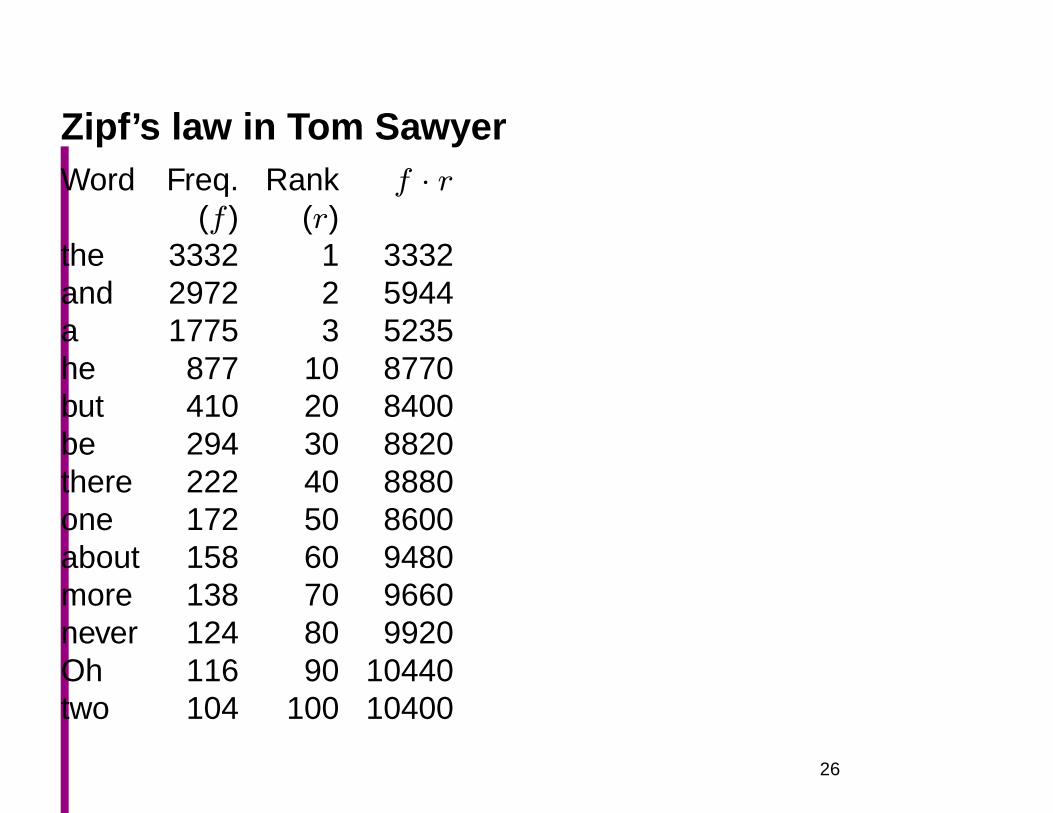
Zipf’s law in Tom SawyerWord Freq. Rank f · r
(f ) (r)the 3332 1 3332and 2972 2 5944a 1775 3 5235he 877 10 8770but 410 20 8400be 294 30 8820there 222 40 8880one 172 50 8600about 158 60 9480more 138 70 9660never 124 80 9920Oh 116 90 10440two 104 100 10400
26
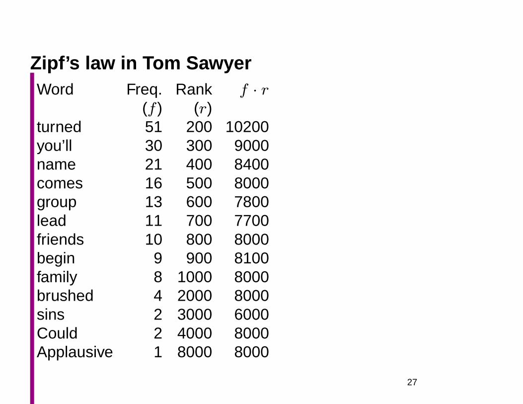
Zipf’s law in Tom SawyerWord Freq. Rank f · r
(f ) (r)turned 51 200 10200you’ll 30 300 9000name 21 400 8400comes 16 500 8000group 13 600 7800lead 11 700 7700friends 10 800 8000begin 9 900 8100family 8 1000 8000brushed 4 2000 8000sins 2 3000 6000Could 2 4000 8000Applausive 1 8000 8000
27
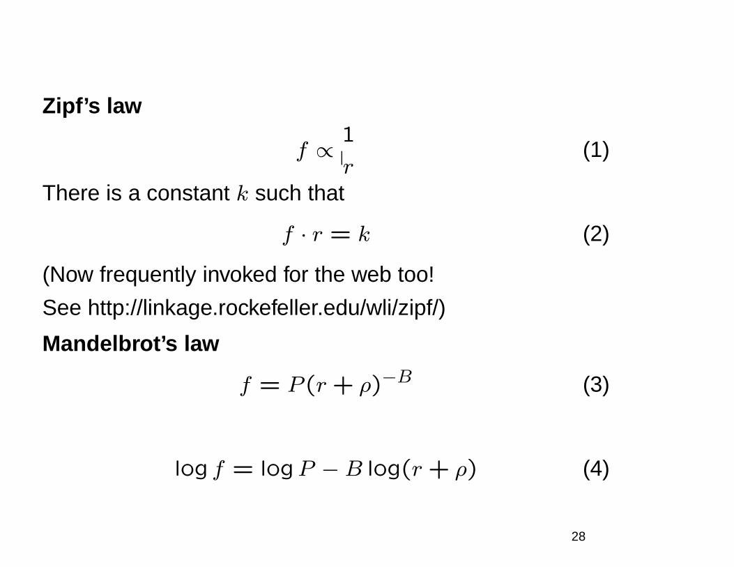
Zipf’s law
f ∝ 1
r(1)
There is a constant k such that
f · r = k (2)
(Now frequently invoked for the web too!
See http://linkage.rockefeller.edu/wli/zipf/)
Mandelbrot’s law
f = P (r+ ρ)−B (3)
log f = logP −B log(r+ ρ) (4)
28
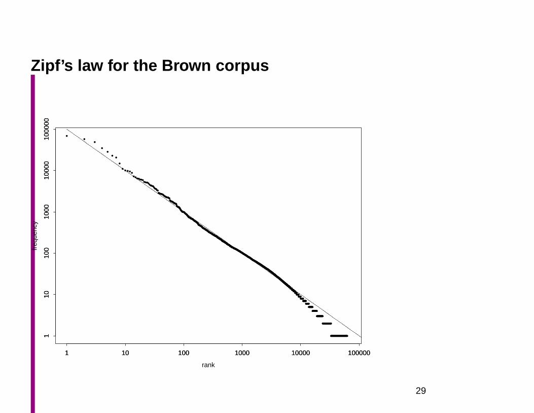
Zipf’s law for the Brown corpus
• • •• •
• •••••••••••••••••••••••••••••••••••••••••••••••••••••••••••••••••••••••••••••••••••••••••••••••••••••••••••••••••••••••••••••••••••••••••••••••••••••••••••••••••••••••••••••••••••••••••••••••••••••••••••••••••••••••••••••••••••••••••••••••••••••••••••••••••••••••••••••••••••••••••••••••••••••••••••••••••••••••••••••••••••••••••••••••••••••••••••••••••••••••••••••••••••••••••••••••••••••••••••••••••••••••••••••••••••••••••••••••••••••••••••••••••••••••••••••••••••••••••••••••••••••••••••••••••••••••••••••••••••••••••••••••••••••••••••••••••••••••••••••••••••••••••••••••••••••••••••••••••••••••••••••••••••••••••••••••••••••••••••••••••••••••••••••••••••••••••••••••••••••••••••••••••••••••••••••••••••••••••••••••••••••••••••••••••••••••••••••••••••••••••••••••••••••••••••••••••••••••••••••••••••••••••••••••••••••••••••••••••••••••••••••••••••••••••••••••••••••••••••••••••••••••••••••••••••••••••••••••••••••••••••••••••••••••••••••••••••••••••••••••••••••••••••••••••••••••••••••••••••••••••••••••••••••••••••••••••••••••••••••••••••••••••••••••••••••••••••••••••••••••••••••••••••••••••••••••••••••••••••••••••••••••••••••••••••••••••••••••••••••••••••••••••••••••••••••••••••••••••••••••••••••••••••••••••••••••••••••••••••••••••••••••••••••••••••••••••••••••••••••••••••••••••••••••••••••••••••••••••••••••••••••••••••••••••••••••••••••
•••••••••••••••••••••••••••••••••••••••••••••••••••••••••••••••••••••••••••••••••••••••••••
••••••••••••••••••••••••••••••••••••••••••••••••••••••••••••••••••••••••••
•••••••••••••••••••••••••••••••••••••••••••••••••••••••••••••••••••••••••••••••••••••••••••••••••••••••••••••••••••••••••••••••••••••••••••••••
rank
freq
uenc
y
1 10 100 1000 10000 100000
110
100
1000
1000
010
0000
1 10 100 1000 10000 100000
110
100
1000
1000
010
0000
29
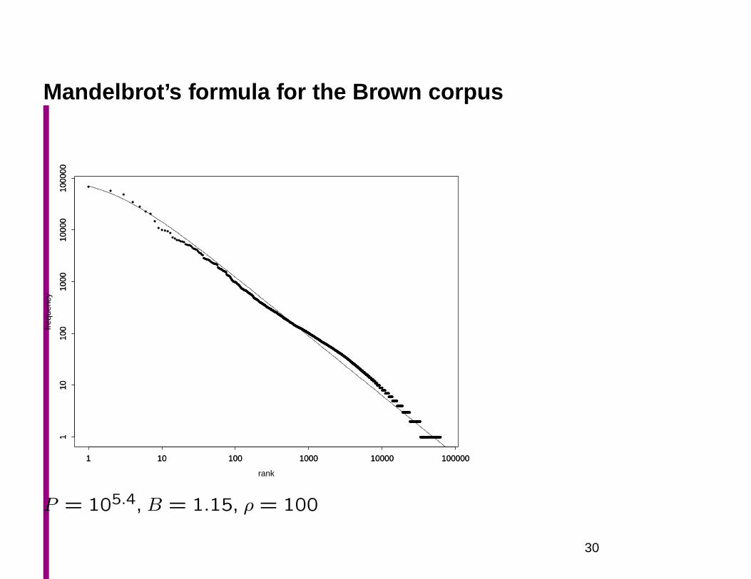
Mandelbrot’s formula for the Brown corpus
• • •• •
• •••••••••••••••••••••••••••••••••••••••••••••••••••••••••••••••••••••••••••••••••••••••••••••••••••••••••••••••••••••••••••••••••••••••••••••••••••••••••••••••••••••••••••••••••••••••••••••••••••••••••••••••••••••••••••••••••••••••••••••••••••••••••••••••••••••••••••••••••••••••••••••••••••••••••••••••••••••••••••••••••••••••••••••••••••••••••••••••••••••••••••••••••••••••••••••••••••••••••••••••••••••••••••••••••••••••••••••••••••••••••••••••••••••••••••••••••••••••••••••••••••••••••••••••••••••••••••••••••••••••••••••••••••••••••••••••••••••••••••••••••••••••••••••••••••••••••••••••••••••••••••••••••••••••••••••••••••••••••••••••••••••••••••••••••••••••••••••••••••••••••••••••••••••••••••••••••••••••••••••••••••••••••••••••••••••••••••••••••••••••••••••••••••••••••••••••••••••••••••••••••••••••••••••••••••••••••••••••••••••••••••••••••••••••••••••••••••••••••••••••••••••••••••••••••••••••••••••••••••••••••••••••••••••••••••••••••••••••••••••••••••••••••••••••••••••••••••••••••••••••••••••••••••••••••••••••••••••••••••••••••••••••••••••••••••••••••••••••••••••••••••••••••••••••••••••••••••••••••••••••••••••••••••••••••••••••••••••••••••••••••••••••••••••••••••••••••••••••••••••••••••••••••••••••••••••••••••••••••••••••••••••••••••••••••••••••••••••••••••••••••••••••••••••••••••••••••••••••••••••••••••••••••••••••••••••••••••••
•••••••••••••••••••••••••••••••••••••••••••••••••••••••••••••••••••••••••••••••••••••••••••
••••••••••••••••••••••••••••••••••••••••••••••••••••••••••••••••••••••••••
•••••••••••••••••••••••••••••••••••••••••••••••••••••••••••••••••••••••••••••••••••••••••••••••••••••••••••••••••••••••••••••••••••••••••••••••
rank
freq
uenc
y
1 10 100 1000 10000 100000
110
100
1000
1000
010
0000
1 10 100 1000 10000 100000
110
100
1000
1000
010
0000
P = 105.4, B = 1.15, ρ = 100
30
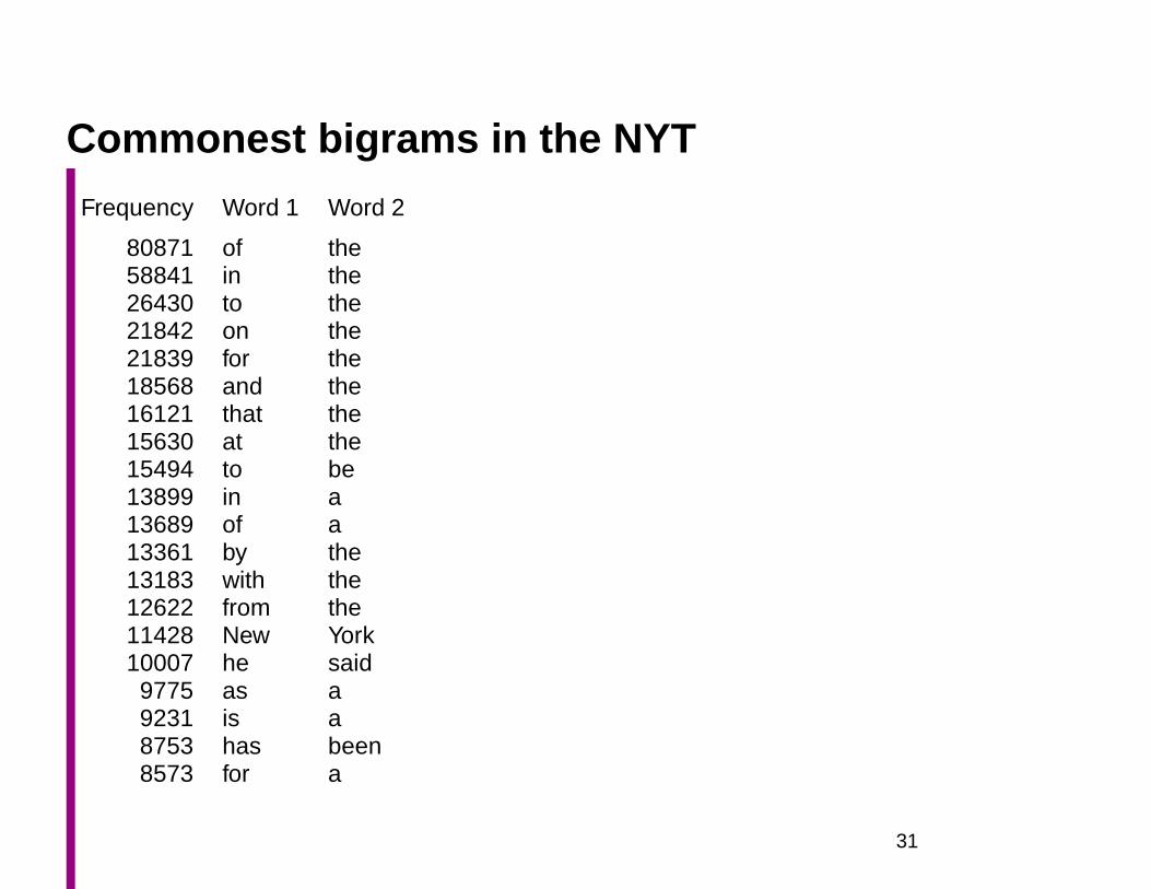
Commonest bigrams in the NYT
Frequency Word 1 Word 2
80871 of the58841 in the26430 to the21842 on the21839 for the18568 and the16121 that the15630 at the15494 to be13899 in a13689 of a13361 by the13183 with the12622 from the11428 New York10007 he said9775 as a9231 is a8753 has been8573 for a
31
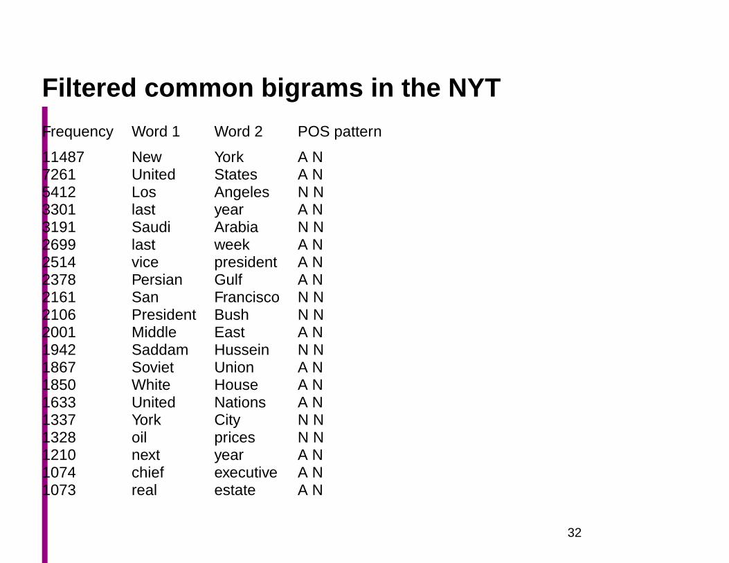
Filtered common bigrams in the NYT
Frequency Word 1 Word 2 POS pattern
11487 New York A N7261 United States A N5412 Los Angeles N N3301 last year A N3191 Saudi Arabia N N2699 last week A N2514 vice president A N2378 Persian Gulf A N2161 San Francisco N N2106 President Bush N N2001 Middle East A N1942 Saddam Hussein N N1867 Soviet Union A N1850 White House A N1633 United Nations A N1337 York City N N1328 oil prices N N1210 next year A N1074 chief executive A N1073 real estate A N
32
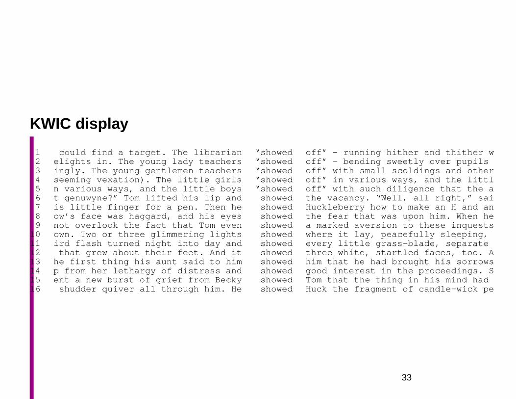
KWIC display
1 could find a target. The librarian “showed off” - running hi ther and thither w2 elights in. The young lady teachers “showed off” - bending s weetly over pupils3 ingly. The young gentlemen teachers “showed off” with smal l scoldings and other4 seeming vexation). The little girls “showed off” in variou s ways, and the littl5 n various ways, and the little boys “showed off” with such di ligence that the a6 t genuwyne?” Tom lifted his lip and showed the vacancy. “Wel l, all right,” sai7 is little finger for a pen. Then he showed Huckleberry how to make an H and an8 ow’s face was haggard, and his eyes showed the fear that was u pon him. When he9 not overlook the fact that Tom even showed a marked aversion to these inquests
10 own. Two or three glimmering lights showed where it lay, pe acefully sleeping,11 ird flash turned night into day and showed every little gra ss-blade, separate12 that grew about their feet. And it showed three white, star tled faces, too. A13 he first thing his aunt said to him showed him that he had bro ught his sorrows14 p from her lethargy of distress and showed good interest in the proceedings. S15 ent a new burst of grief from Becky showed Tom that the thing in his mind had16 shudder quiver all through him. He showed Huck the fragmen t of candle-wick pe
33
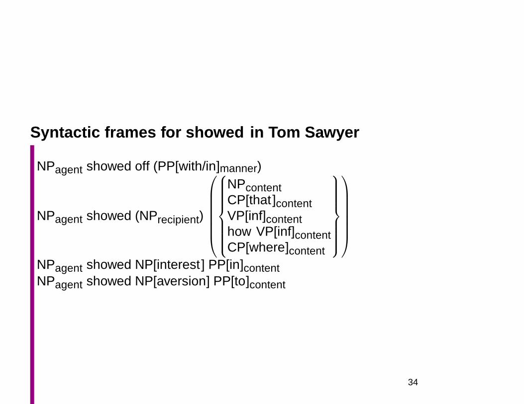
Syntactic frames for showed in Tom Sawyer
NPagent showed off (PP[with/in]manner)
NPagent showed (NPrecipient)
NPcontentCP[that ]contentVP[inf]contenthow VP[inf]contentCP[where]content
NPagent showed NP[interest ] PP[in]contentNPagent showed NP[aversion] PP[to]content
34
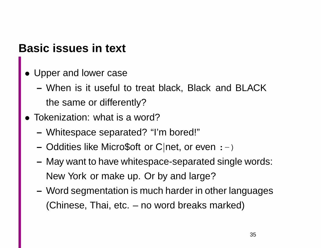
Basic issues in text
• Upper and lower case
– When is it useful to treat black, Black and BLACK
the same or differently?
• Tokenization: what is a word?
– Whitespace separated? “I’m bored!”
– Oddities like Micro$oft or C|net, or even :-)
– May want to have whitespace-separated single words:
New York or make up. Or by and large?
– Word segmentation is much harder in other languages
(Chinese, Thai, etc. – no word breaks marked)
35
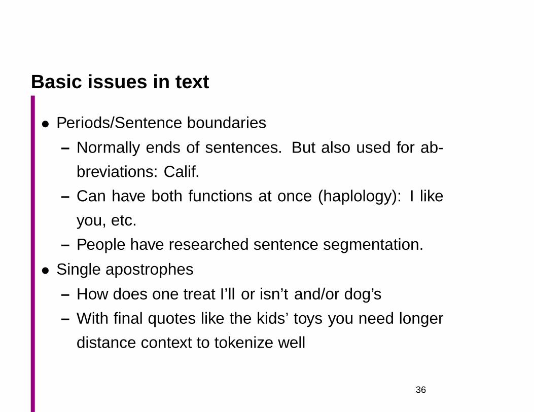
Basic issues in text
• Periods/Sentence boundaries
– Normally ends of sentences. But also used for ab-
breviations: Calif.
– Can have both functions at once (haplology): I like
you, etc.
– People have researched sentence segmentation.
• Single apostrophes
– How does one treat I’ll or isn’t and/or dog’s
– With final quotes like the kids’ toys you need longer
distance context to tokenize well
36
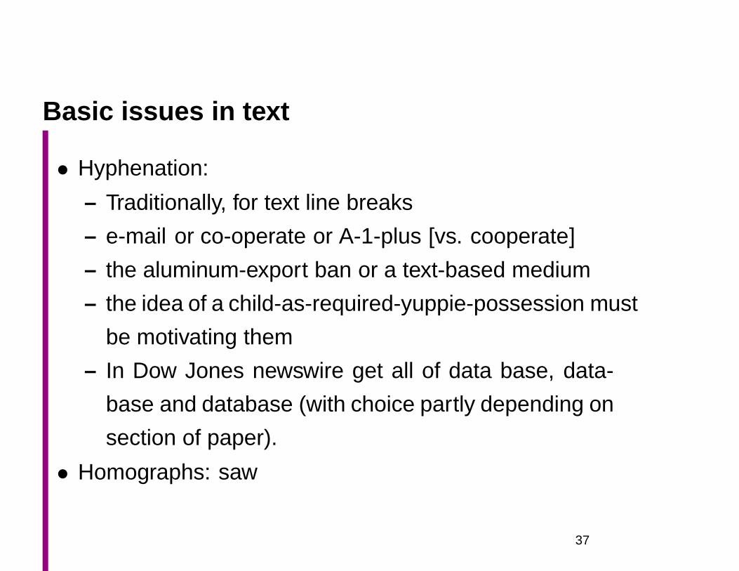
Basic issues in text
• Hyphenation:
– Traditionally, for text line breaks
– e-mail or co-operate or A-1-plus [vs. cooperate]
– the aluminum-export ban or a text-based medium
– the idea of a child-as-required-yuppie-possession must
be motivating them
– In Dow Jones newswire get all of data base, data-
base and database (with choice partly depending on
section of paper).
• Homographs: saw
37
Much of the structure is implicit, traditionally
• Two carriage returns indicate a paragrah break
• Now, often SGML or XML gives at least some of the
macro structure (sentences, paragraphs). Commonly
not micro-structure
• <p><s>And then he left.</s>
<s>He did not say another word.</s></p>
• <utt speak="Fred" date="10-Feb-1998">That
is an ugly couch.</utt>
• May not be semantic markup:
– <B><font="+3">Relevant prior approaches</font></B>
38
Distinctiveness of NLP as an ML problem
• Language allows the complex, compositional encoding
of thoughts, ideas, feelings, . . . , intelligence.
• Most structure is hidden
• Relational, constraint satisfaction nature
• Long pipelines
• Large and strange, sparse, discrete distributions
• Large scale
• Feature-driven; performance-driven
39
Distinctiveness of NLP as an ML problem
• Much hidden structure; long processing pipelines
– Long pipelines of probabilistic decompositions,
through which errors can – and do – propagate
– The problem has a relational/CSP nature. It’s not
just doing a series of (assumed iid) simple classifica-
tion tasks. There are a lot of decisions to coordinate.
– We are often dealing with hierarchical structures (branch-
ing processes), and often want to allow more com-
plex forms of information sharing (dependencies/relational
structure).
40
NLP: Large, sparse, discrete distributions
• Both features and assigned classes regularly involve
multinomial distributions over huge numbers of values
(often in the tens of thousands).
• The distributions are very uneven, and have fat tails
• Enormous problems with data sparseness: much work
on smoothing distributions/backoff (shrinkage), etc.
• We normally have inadequate (labeled) data to esti-
mate probabilities
• Unknown/unseen things are usually a central problem
• Generally dealing with discrete distributions though
41
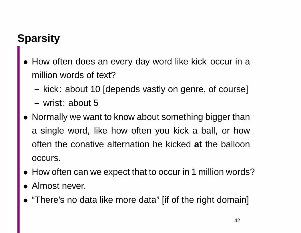
Sparsity
• How often does an every day word like kick occur in a
million words of text?
– kick : about 10 [depends vastly on genre, of course]
– wrist : about 5
• Normally we want to know about something bigger than
a single word, like how often you kick a ball, or how
often the conative alternation he kicked at the balloon
occurs.
• How often can we expect that to occur in 1 million words?
• Almost never.
• “There’s no data like more data” [if of the right domain]
42
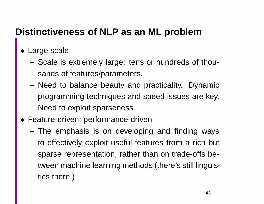
Distinctiveness of NLP as an ML problem
• Large scale
– Scale is extremely large: tens or hundreds of thou-sands of features/parameters.
– Need to balance beauty and practicality. Dynamicprogramming techniques and speed issues are key.Need to exploit sparseness.
• Feature-driven; performance-driven
– The emphasis is on developing and finding waysto effectively exploit useful features from a rich butsparse representation, rather than on trade-offs be-tween machine learning methods (there’s still linguis-tics there!)
43
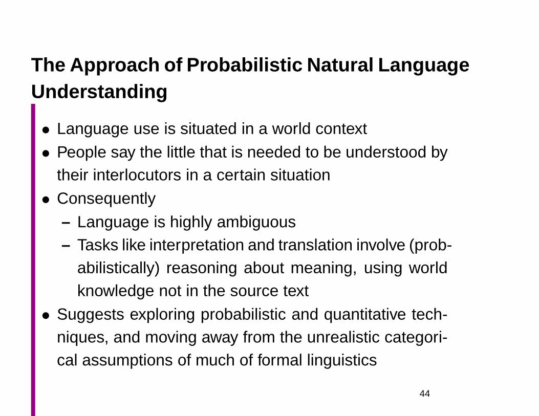
The Approach of Probabilistic Natural LanguageUnderstanding
• Language use is situated in a world context
• People say the little that is needed to be understood bytheir interlocutors in a certain situation
• Consequently
– Language is highly ambiguous– Tasks like interpretation and translation involve (prob-
abilistically) reasoning about meaning, using worldknowledge not in the source text
• Suggests exploring probabilistic and quantitative tech-niques, and moving away from the unrealistic categori-cal assumptions of much of formal linguistics
44
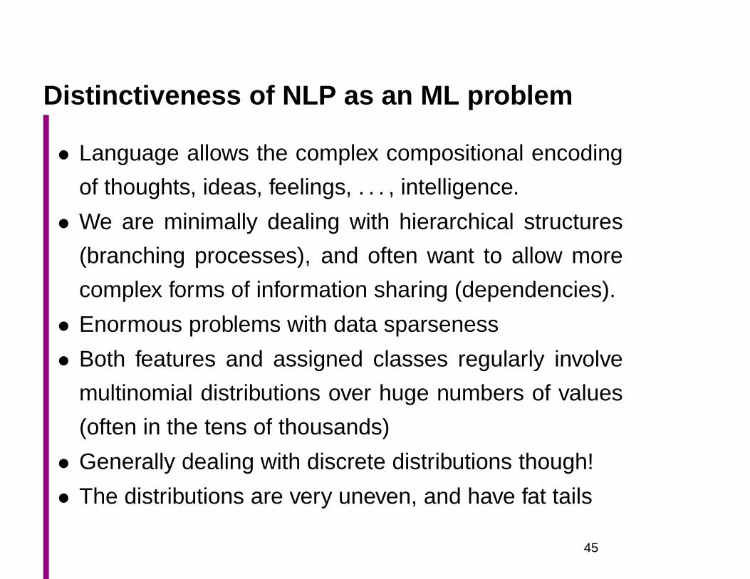
Distinctiveness of NLP as an ML problem
• Language allows the complex compositional encoding
of thoughts, ideas, feelings, . . . , intelligence.
• We are minimally dealing with hierarchical structures
(branching processes), and often want to allow more
complex forms of information sharing (dependencies).
• Enormous problems with data sparseness
• Both features and assigned classes regularly involve
multinomial distributions over huge numbers of values
(often in the tens of thousands)
• Generally dealing with discrete distributions though!
• The distributions are very uneven, and have fat tails
45
Frequencies of frequencies in Tom Sawyer
Word Frequency ofFrequency Frequency
1 3993 71,730 word tokens2 1292 8,018 word types3 6644 4105 2436 1997 1728 1319 82
10 9111–50 540
51–100 99> 100 102
46
The obligatory Zipf’s law slide:
Zipf’s law for the Brown corpus
• • •• •
• •••••••••••••••••••••••••••••••••••••••••••••••••••••••••••••••••••••••••••••••••••••••••••••••••••••••••••••••••••••••••••••••••••••••••••••••••••••••••••••••••••••••••••••••••••••••••••••••••••••••••••••••••••••••••••••••••••••••••••••••••••••••••••••••••••••••••••••••••••••••••••••••••••••••••••••••••••••••••••••••••••••••••••••••••••••••••••••••••••••••••••••••••••••••••••••••••••••••••••••••••••••••••••••••••••••••••••••••••••••••••••••••••••••••••••••••••••••••••••••••••••••••••••••••••••••••••••••••••••••••••••••••••••••••••••••••••••••••••••••••••••••••••••••••••••••••••••••••••••••••••••••••••••••••••••••••••••••••••••••••••••••••••••••••••••••••••••••••••••••••••••••••••••••••••••••••••••••••••••••••••••••••••••••••••••••••••••••••••••••••••••••••••••••••••••••••••••••••••••••••••••••••••••••••••••••••••••••••••••••••••••••••••••••••••••••••••••••••••••••••••••••••••••••••••••••••••••••••••••••••••••••••••••••••••••••••••••••••••••••••••••••••••••••••••••••••••••••••••••••••••••••••••••••••••••••••••••••••••••••••••••••••••••••••••••••••••••••••••••••••••••••••••••••••••••••••••••••••••••••••••••••••••••••••••••••••••••••••••••••••••••••••••••••••••••••••••••••••••••••••••••••••••••••••••••••••••••••••••••••••••••••••••••••••••••••••••••••••••••••••••••••••••••••••••••••••••••••••••••••••••••••••••••••••••••••••••••••
•••••••••••••••••••••••••••••••••••••••••••••••••••••••••••••••••••••••••••••••••••••••••••
••••••••••••••••••••••••••••••••••••••••••••••••••••••••••••••••••••••••••
•••••••••••••••••••••••••••••••••••••••••••••••••••••••••••••••••••••••••••••••••••••••••••••••••••••••••••••••••••••••••••••••••••••••••••••••
rank
freq
uenc
y
1 10 100 1000 10000 100000
110
100
1000
1000
010
0000
1 10 100 1000 10000 100000
110
100
1000
1000
010
0000
47
Zipf’s law
f ∝ 1
ror, there is a k such that f · r = k
(Now frequently invoked for the web too!
See http://linkage.rockefeller.edu/wli/zipf/)
Mandelbrot’s law
f = P (r+ ρ)−B
log f = logP −B log(r+ ρ)
48
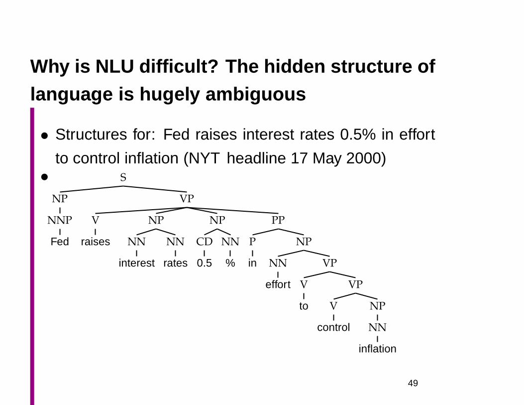
Why is NLU difficult? The hidden structure oflanguage is hugely ambiguous
• Structures for: Fed raises interest rates 0.5% in effort
to control inflation (NYT headline 17 May 2000)• S
NP
NNP
Fed
VP
V
raises
NP
NN
interest
NN
rates
NP
CD
0.5
NN
%
PP
P
in
NP
NN
effort
VP
V
to
VP
V
control
NP
NN
inflation
49
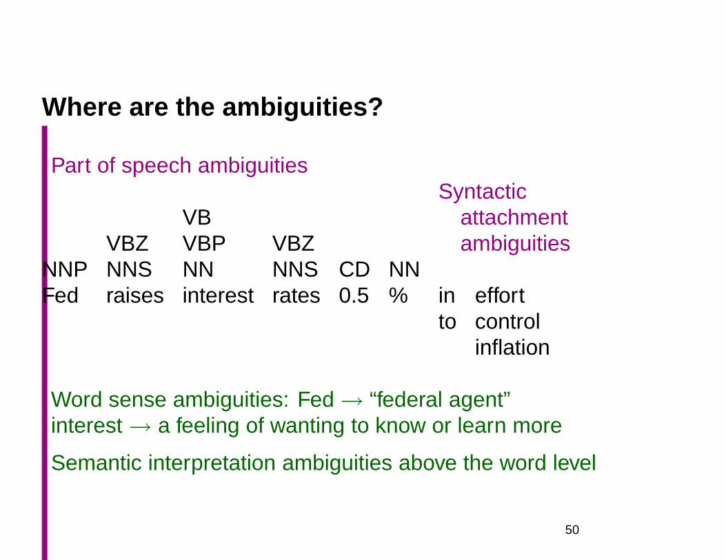
Where are the ambiguities?
Part of speech ambiguitiesSyntactic
VB attachmentVBZ VBP VBZ ambiguities
NNP NNS NN NNS CD NNFed raises interest rates 0.5 % in effort
to controlinflation
Word sense ambiguities: Fed→ “federal agent”interest→ a feeling of wanting to know or learn more
Semantic interpretation ambiguities above the word level
50

Mathematical Foundations
FSNLP, chapter 2
Christopher Manning andHinrich Schütze
© 1999–2002
51
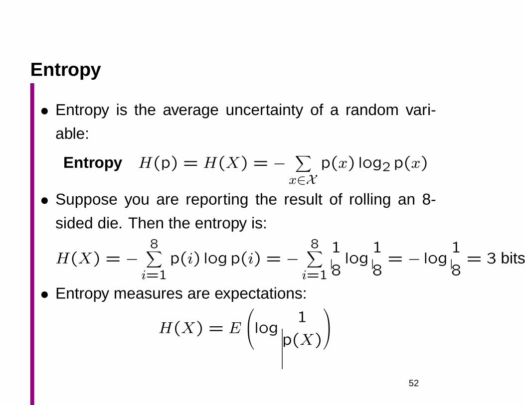
Entropy
• Entropy is the average uncertainty of a random vari-
able:
Entropy H(p) = H(X) = − ∑
x∈Xp(x) log2 p(x)
• Suppose you are reporting the result of rolling an 8-
sided die. Then the entropy is:
H(X) = −8
∑
i=1p(i) logp(i) = −
8∑
i=1
1
8log
1
8= − log
1
8= 3 bits
• Entropy measures are expectations:
H(X) = E
log1
p(X)
52

Simplified Polynesian
• Simplified Polynesian appears to be just a random se-
quence of letters, with the letter frequencies as shown:
• p t k a i u1/8 1/4 1/8 1/4 1/8 1/8
• Then the per-letter entropy is:
H(P ) = −∑
i∈p,t,k,a,i,uP (i) logP (i)
= −[4× 1
8log
1
8+ 2× 1
4log
1
4] = 2
1
2bits
We can design a code that on average takes 212 bits a
letter:p t k a i u100 00 101 01 110 111
53
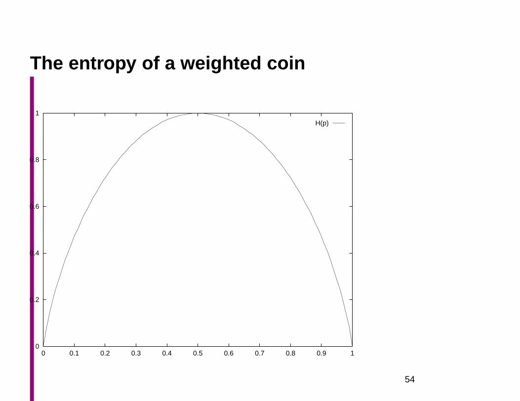
The entropy of a weighted coin
0
0.2
0.4
0.6
0.8
1
0 0.1 0.2 0.3 0.4 0.5 0.6 0.7 0.8 0.9 1
H(p)
54
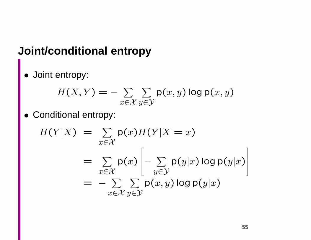
Joint/conditional entropy
• Joint entropy:
H(X, Y ) = − ∑
x∈X
∑
y∈Yp(x, y) logp(x, y)
• Conditional entropy:
H(Y |X) =∑
x∈Xp(x)H(Y |X = x)
=∑
x∈Xp(x)
− ∑
y∈Yp(y|x) log p(y|x)
= − ∑
x∈X
∑
y∈Yp(x, y) log p(y|x)
55
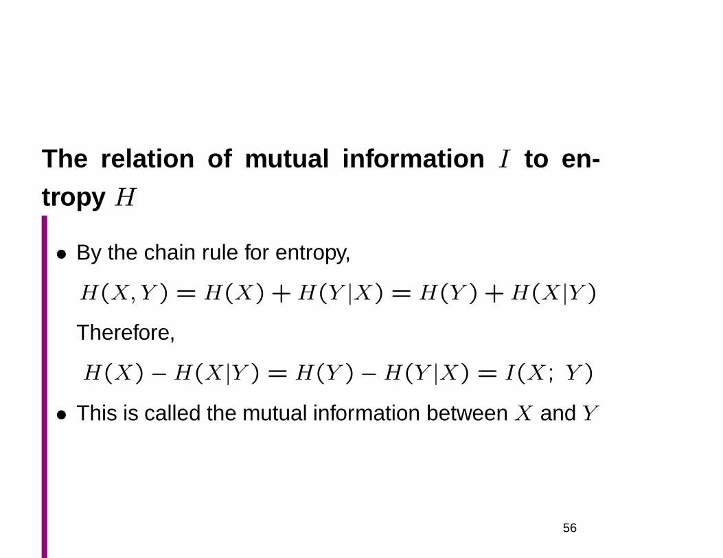
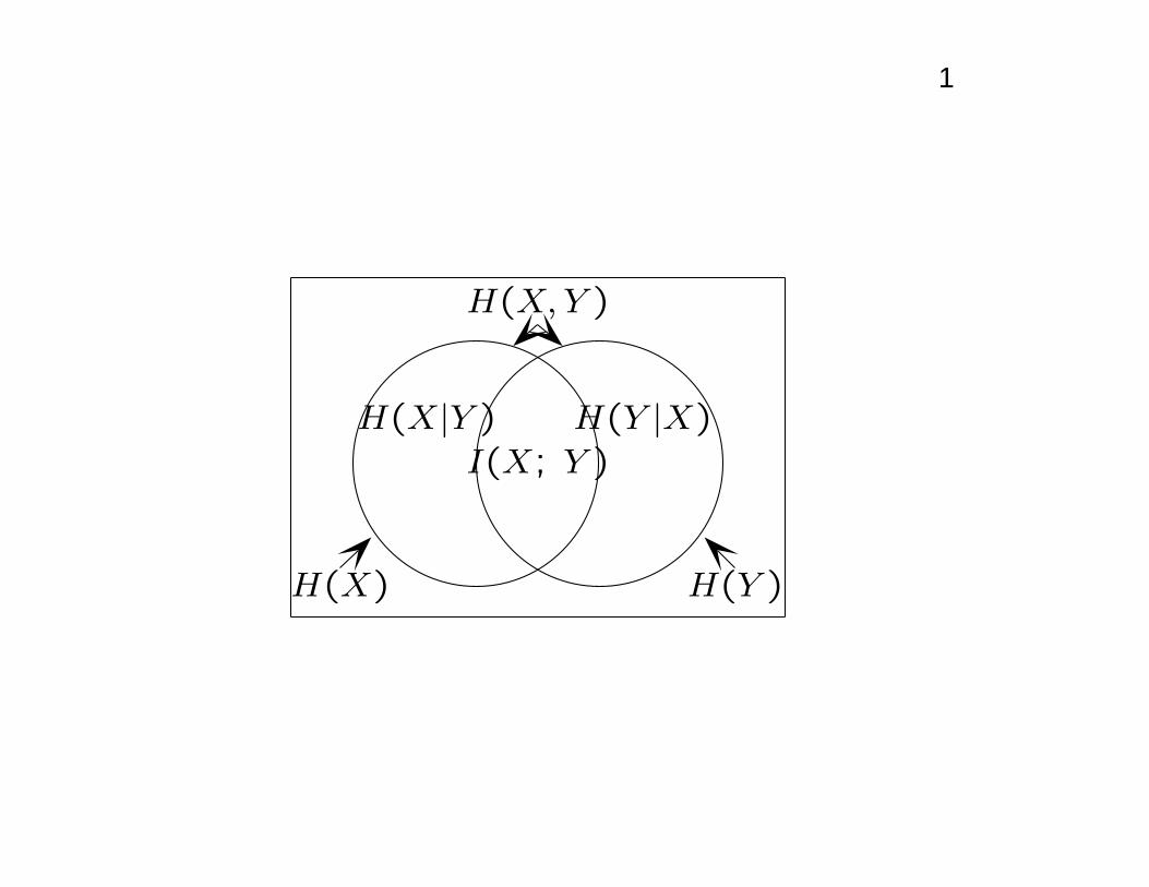
The relation of mutual information I to en-tropy H
• By the chain rule for entropy,
H(X, Y ) = H(X) +H(Y |X) = H(Y ) +H(X|Y )
Therefore,
H(X)−H(X|Y ) = H(Y )−H(Y |X) = I(X; Y )
• This is called the mutual information between X and Y
56
1
I(X; Y )
H(X|Y ) H(Y |X)
H(X) H(Y )
H(X,Y )
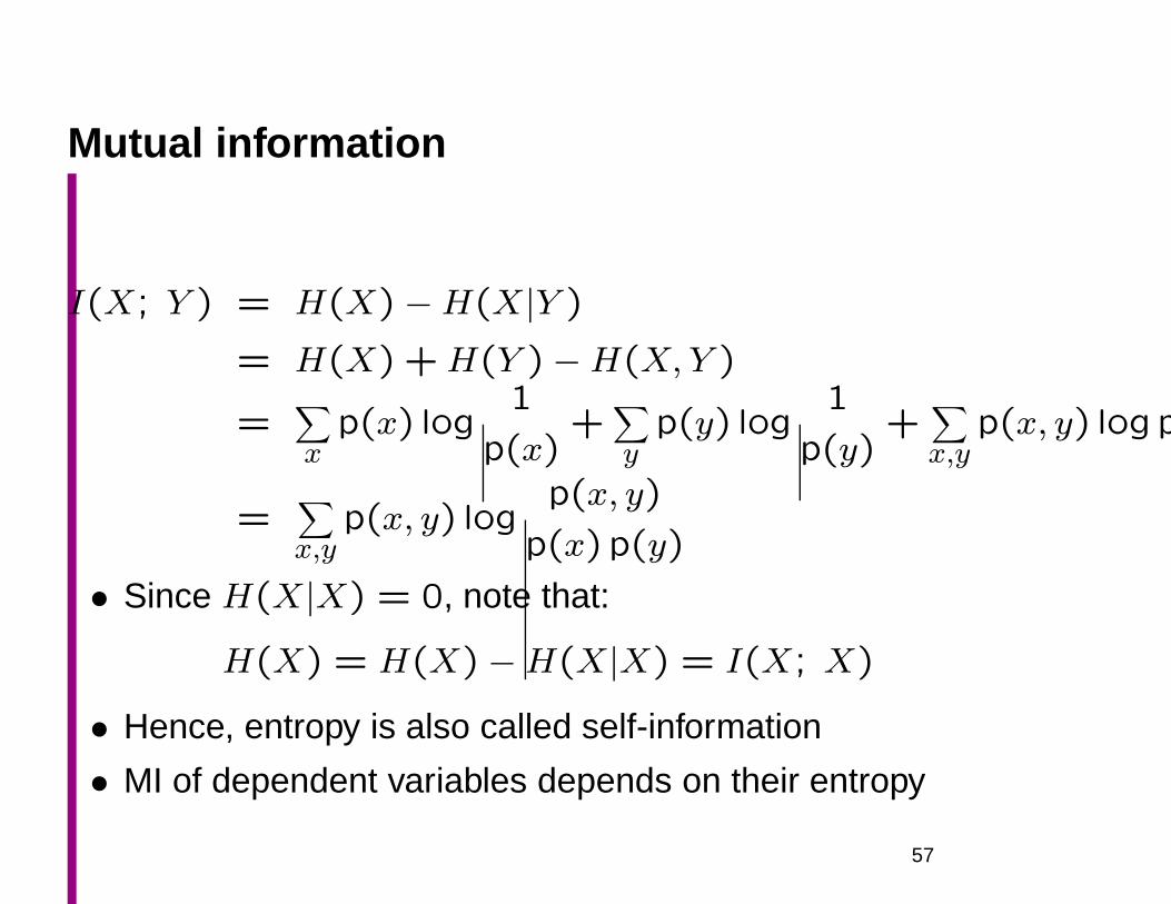
Mutual information
I(X; Y ) = H(X)−H(X|Y )
= H(X) +H(Y )−H(X, Y )
=∑
xp(x) log
1
p(x)+
∑
yp(y) log
1
p(y)+
∑
x,yp(x, y) logp(
=∑
x,yp(x, y) log
p(x, y)
p(x) p(y)
• Since H(X|X) = 0, note that:
H(X) = H(X)−H(X|X) = I(X; X)
• Hence, entropy is also called self-information
• MI of dependent variables depends on their entropy
57
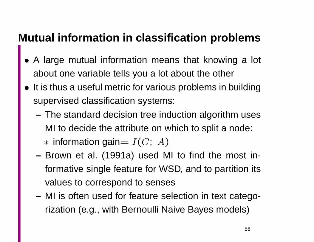
Mutual information in classification problems
• A large mutual information means that knowing a lotabout one variable tells you a lot about the other
• It is thus a useful metric for various problems in buildingsupervised classification systems:
– The standard decision tree induction algorithm usesMI to decide the attribute on which to split a node:∗ information gain= I(C; A)
– Brown et al. (1991a) used MI to find the most in-formative single feature for WSD, and to partition itsvalues to correspond to senses
– MI is often used for feature selection in text catego-rization (e.g., with Bernoulli Naive Bayes models)
58
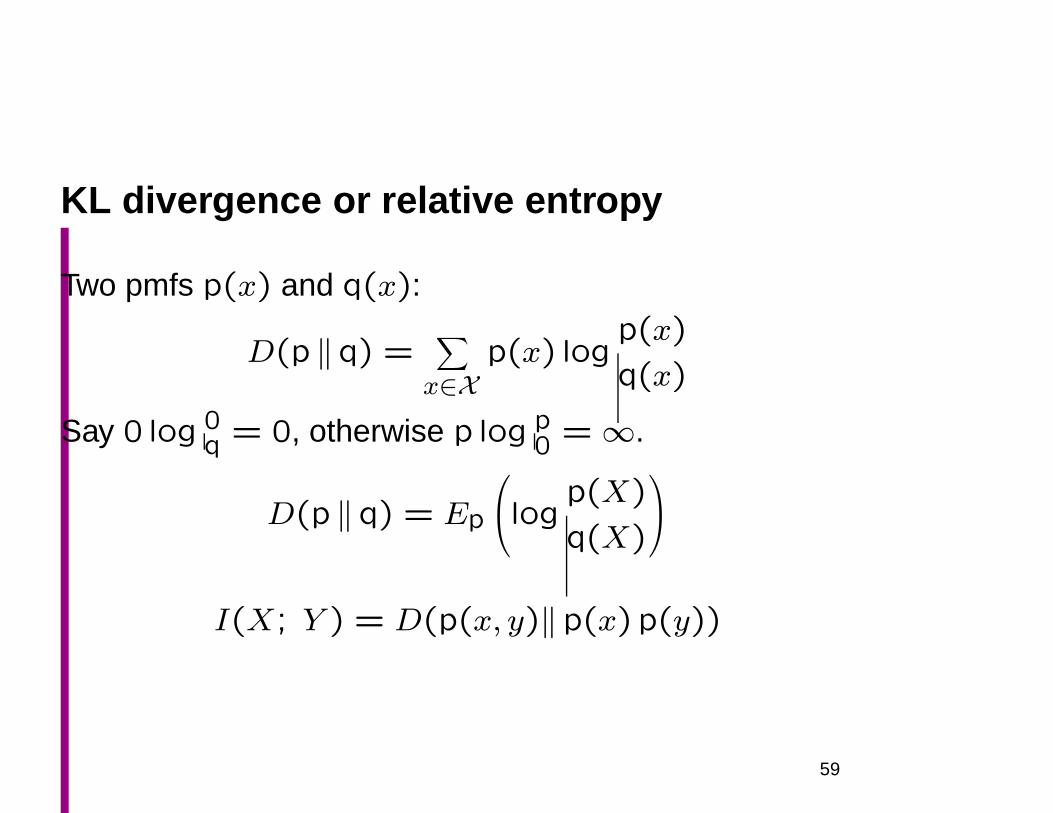
KL divergence or relative entropy
Two pmfs p(x) and q(x):
D(p ‖q) =∑
x∈Xp(x) log
p(x)
q(x)
Say 0 log 0q = 0, otherwise p log p
0 =∞.
D(p ‖q) = Ep
logp(X)
q(X)
I(X; Y ) = D(p(x, y)‖p(x) p(y))
59
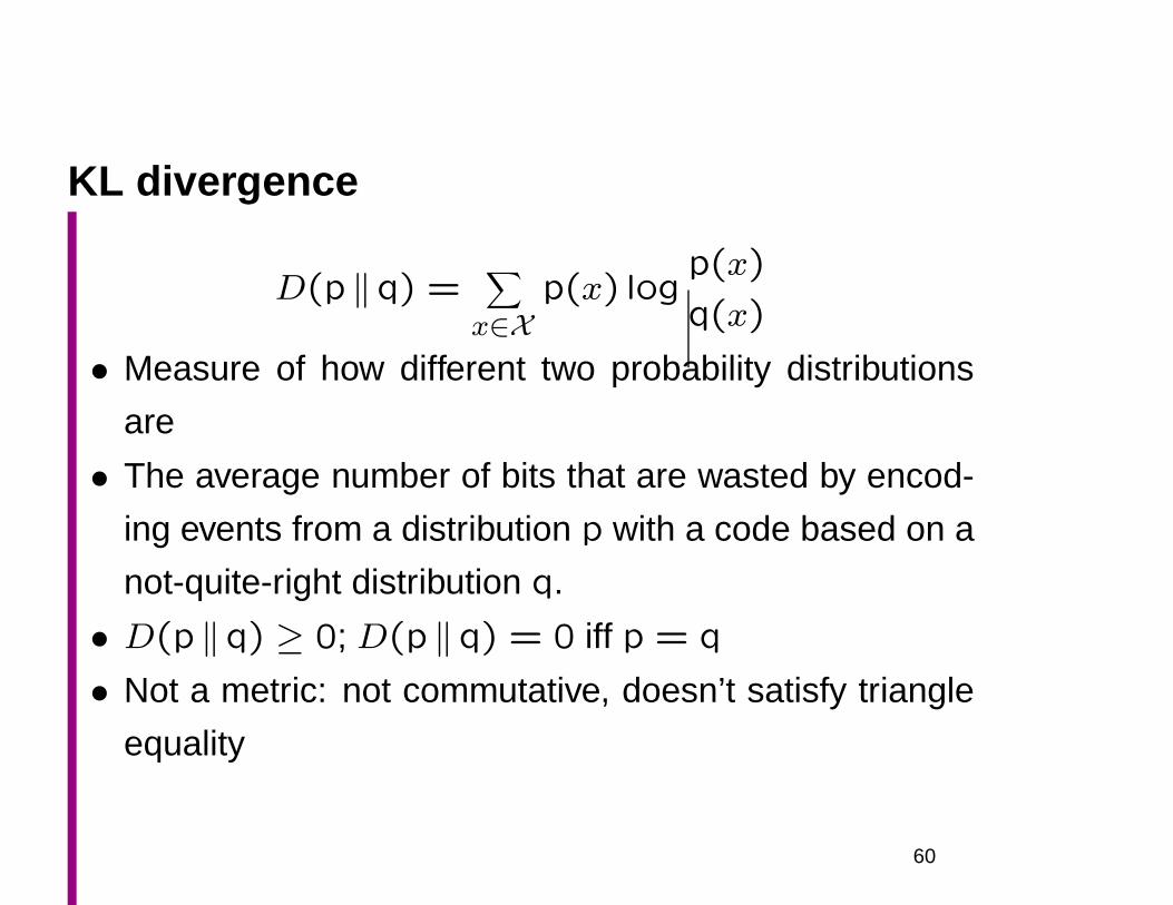
KL divergence
D(p ‖q) =∑
x∈Xp(x) log
p(x)
q(x)
• Measure of how different two probability distributions
are
• The average number of bits that are wasted by encod-
ing events from a distribution p with a code based on a
not-quite-right distribution q.
• D(p ‖q) ≥ 0; D(p ‖q) = 0 iff p = q
• Not a metric: not commutative, doesn’t satisfy triangle
equality
60
[Slide on D(p‖q) vs. D(q‖p)]
61
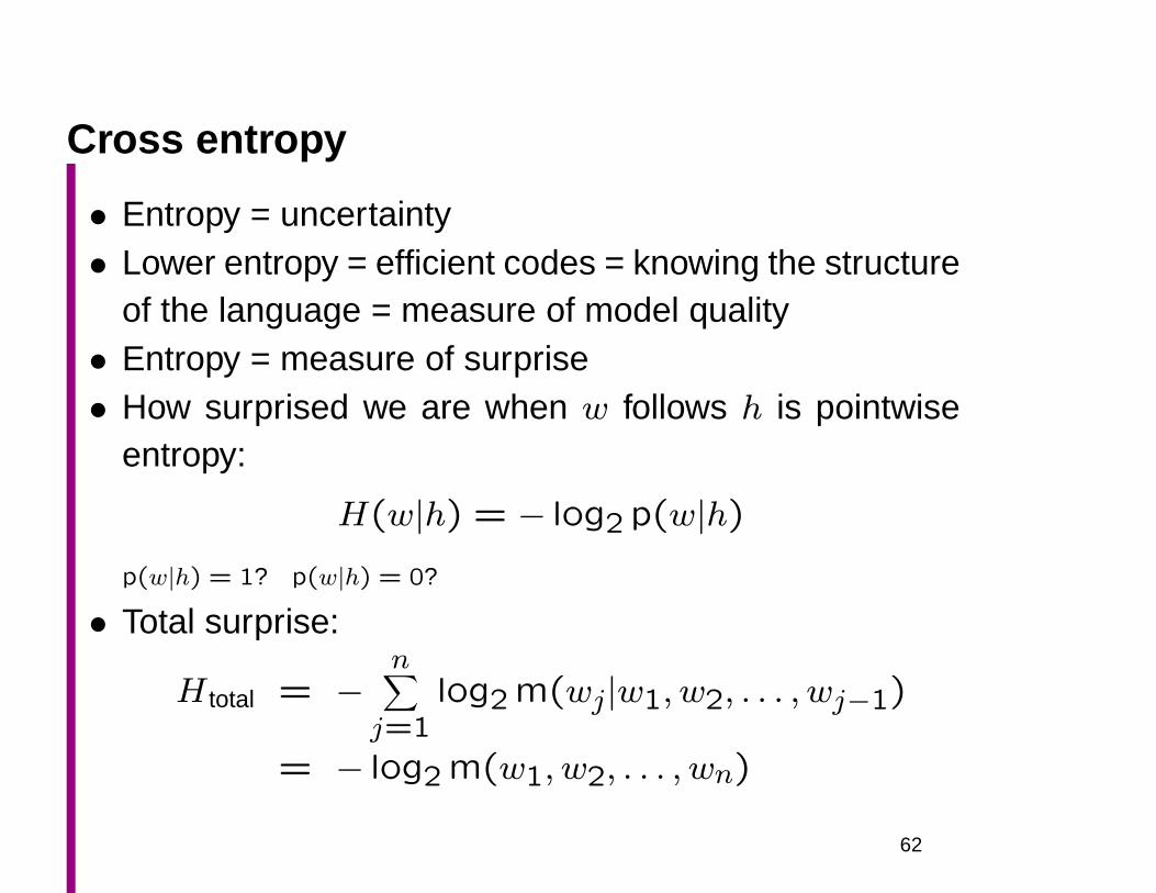
Cross entropy
• Entropy = uncertainty• Lower entropy = efficient codes = knowing the structure
of the language = measure of model quality• Entropy = measure of surprise• How surprised we are when w follows h is pointwise
entropy:
H(w|h) = − log2 p(w|h)p(w|h) = 1? p(w|h) = 0?
• Total surprise:
H total = −n
∑
j=1log2 m(wj|w1, w2, . . . , wj−1)
= − log2 m(w1, w2, . . . , wn)
62
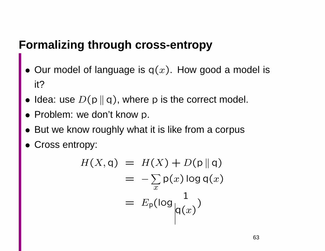
Formalizing through cross-entropy
• Our model of language is q(x). How good a model is
it?
• Idea: use D(p ‖q), where p is the correct model.
• Problem: we don’t know p.
• But we know roughly what it is like from a corpus
• Cross entropy:
H(X,q) = H(X) +D(p ‖q)
= −∑
xp(x) log q(x)
= Ep(log1
q(x))
63
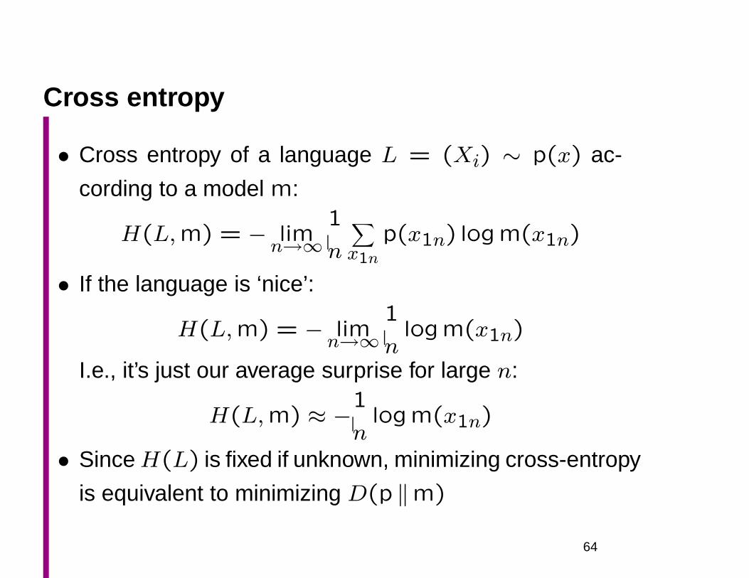
Cross entropy
• Cross entropy of a language L = (Xi) ∼ p(x) ac-
cording to a model m:
H(L,m) = − limn→∞
1
n
∑
x1np(x1n) logm(x1n)
• If the language is ‘nice’:
H(L,m) = − limn→∞
1
nlogm(x1n)
I.e., it’s just our average surprise for large n:
H(L,m) ≈ −1
nlogm(x1n)
• SinceH(L) is fixed if unknown, minimizing cross-entropy
is equivalent to minimizing D(p ‖m)
64
1
• Assuming: independent test data, L = (Xi) is sta-
tionary [does’t change over time], ergodic [doesn’t get
stuck]
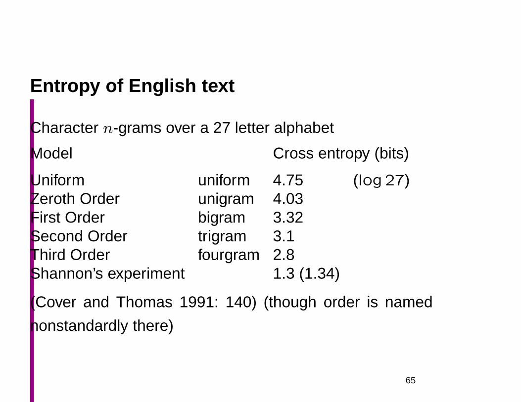
Entropy of English text
Character n-grams over a 27 letter alphabet
Model Cross entropy (bits)
Uniform uniform 4.75 (log 27)Zeroth Order unigram 4.03First Order bigram 3.32Second Order trigram 3.1Third Order fourgram 2.8Shannon’s experiment 1.3 (1.34)
(Cover and Thomas 1991: 140) (though order is named
nonstandardly there)
65
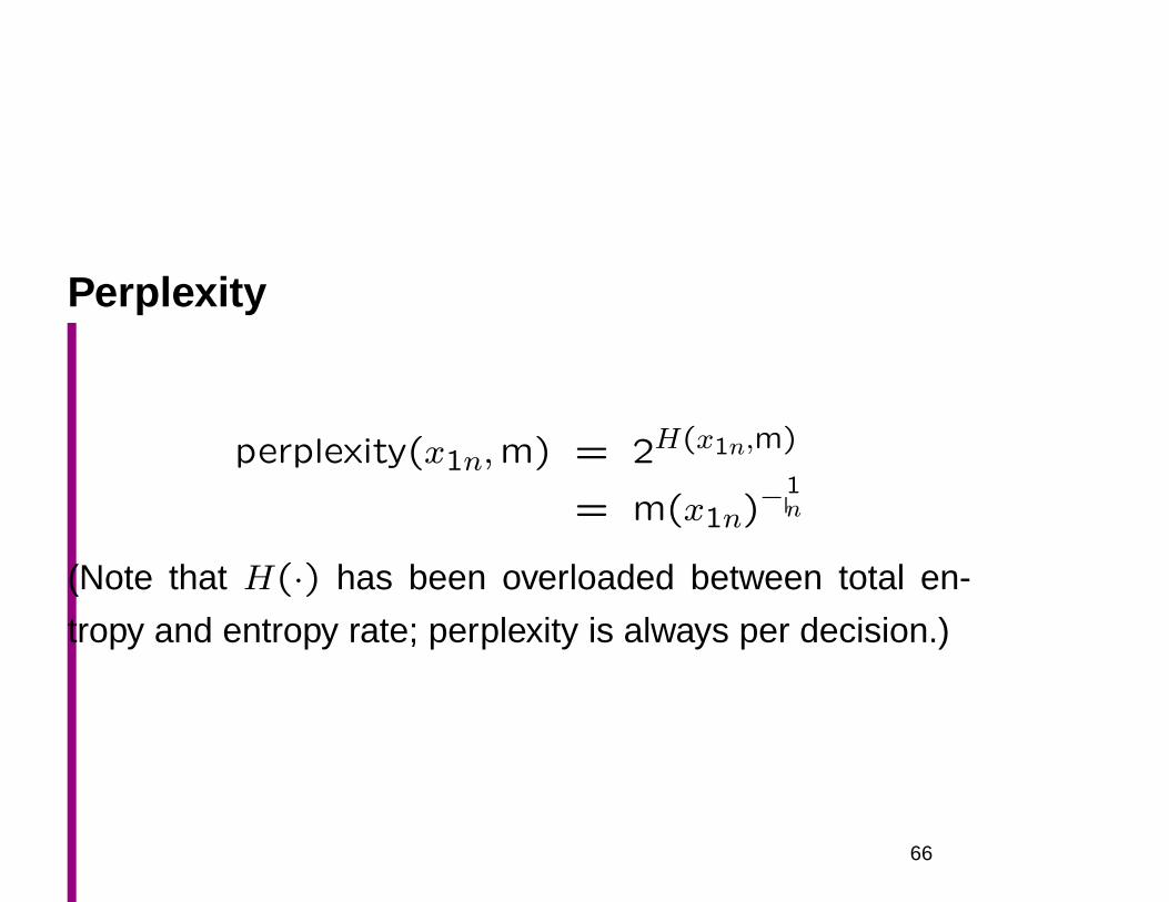
Perplexity
perplexity(x1n,m) = 2H(x1n,m)
= m(x1n)−1n
(Note that H(·) has been overloaded between total en-
tropy and entropy rate; perplexity is always per decision.)
66
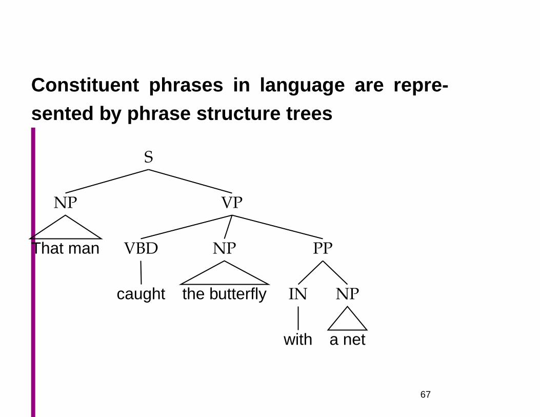
Constituent phrases in language are repre-sented by phrase structure trees
S
NP
That man
VP
VBD
caught
NP
the butterfly
PP
IN
with
NP
a net
67
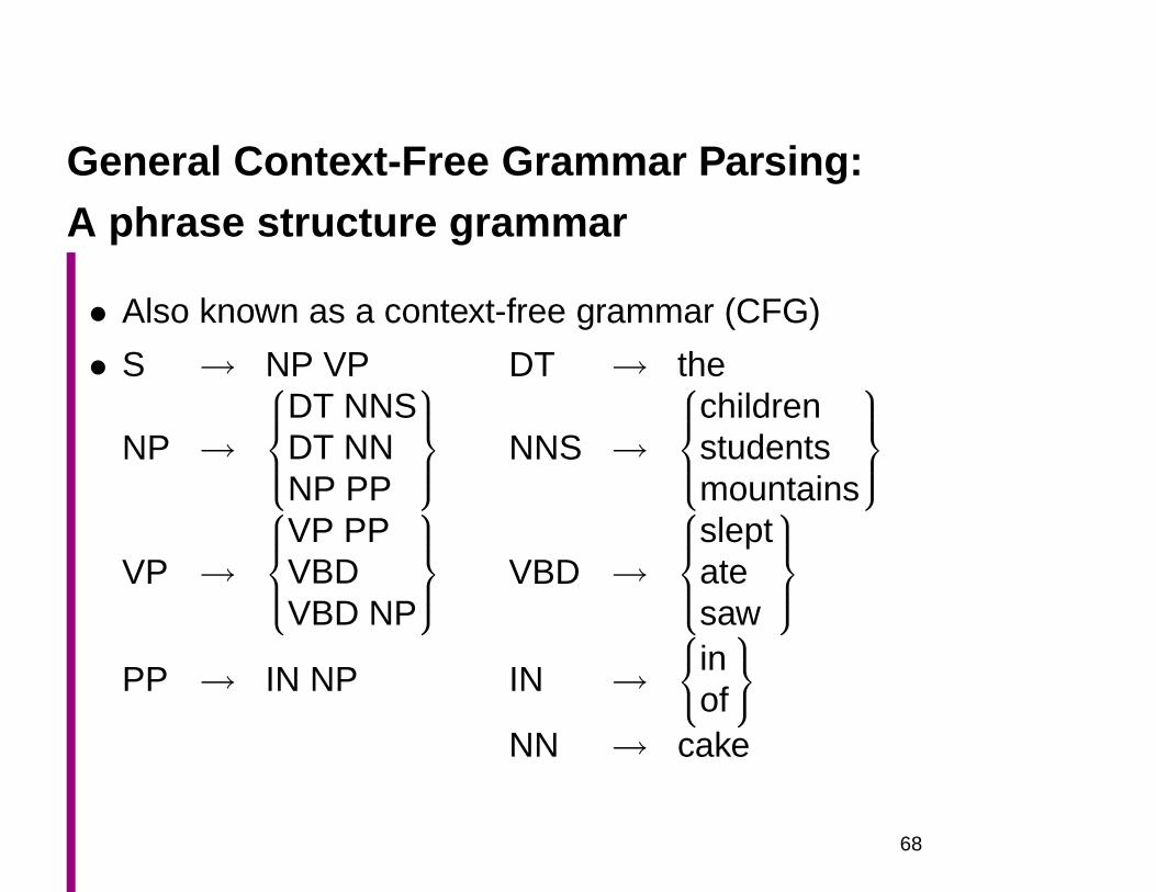
General Context-Free Grammar Parsing:A phrase structure grammar
• Also known as a context-free grammar (CFG)
• S → NP VP DT → the
NP →
DT NNSDT NNNP PP
NNS →
childrenstudentsmountains
VP →
VP PPVBDVBD NP
VBD →
sleptatesaw
PP → IN NP IN →
inof
NN → cake
68
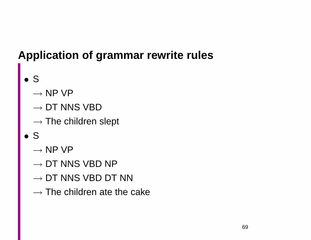
Application of grammar rewrite rules
• S
→ NP VP
→ DT NNS VBD
→ The children slept
• S
→ NP VP
→ DT NNS VBD NP
→ DT NNS VBD DT NN
→ The children ate the cake
69
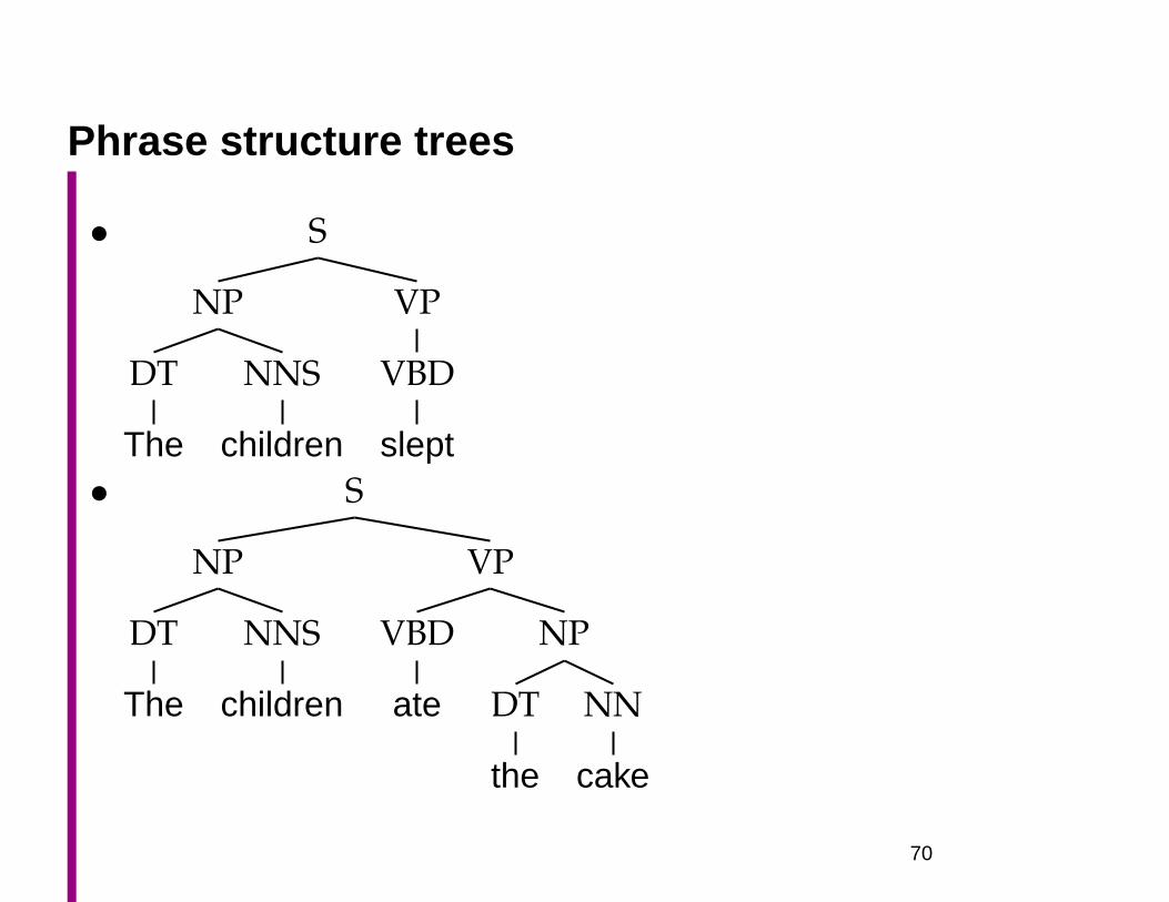
Phrase structure trees
• S
NP
DT
The
NNS
children
VP
VBD
slept• S
NP
DT
The
NNS
children
VP
VBD
ate
NP
DT
the
NN
cake
70
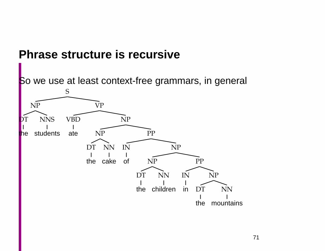
Phrase structure is recursive
So we use at least context-free grammars, in generalS
NP
DT
the
NNS
students
VP
VBD
ate
NP
NP
DT
the
NN
cake
PP
IN
of
NP
NP
DT
the
NN
children
PP
IN
in
NP
DT
the
NN
mountains
71
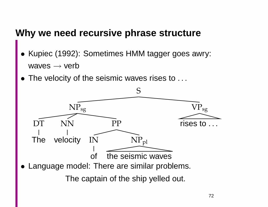
Why we need recursive phrase structure
• Kupiec (1992): Sometimes HMM tagger goes awry:
waves→ verb
• The velocity of the seismic waves rises to . . .
S
NPsg
DT
The
NN
velocity
PP
IN
of
NPpl
the seismic waves
VPsg
rises to . . .
• Language model: There are similar problems.
The captain of the ship yelled out.
72
Why we need phrase structure (2)
• Syntax gives important clues in information extraction
tasks and some cases of named entity recognition
• We have recently demonstrated that stimulation of [CELLTYPEhuman
T and natural killer cells] with [PROTEINIL-12] induces
tyrosine phosphorylation of the [PROTEINJanus family
tyrosine kinase] [PROTEINJAK2] and [PROTEINTyk2].
• Things that are the object of phosphorylate are likely
proteins.
73

Constituency
• Phrase structure organizes words into nested constituents.
• How do we know what is a constituent? (Not that lin-
guists don’t argue about some cases.)
– Distribution: behaves as a unit that appears in differ-
ent places:
∗ John talked [to the children] [about drugs].
∗ John talked [about drugs] [to the children].
∗ *John talked drugs to the children about
– Substitution/expansion/pro-forms:
∗ I sat [on the box/right on top of the box/there].
– Coordination, no intrusion, fragments, semantics, . . .
74
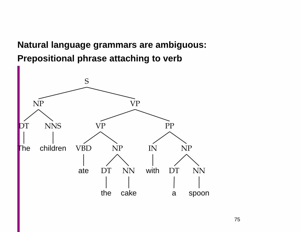
Natural language grammars are ambiguous:
Prepositional phrase attaching to verb
S
NP
DT
The
NNS
children
VP
VP
VBD
ate
NP
DT
the
NN
cake
PP
IN
with
NP
DT
a
NN
spoon
75
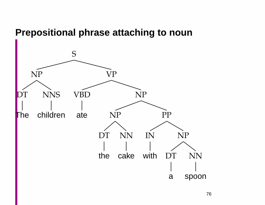
Prepositional phrase attaching to noun
S
NP
DT
The
NNS
children
VP
VBD
ate
NP
NP
DT
the
NN
cake
PP
IN
with
NP
DT
a
NN
spoon
76

Attachment ambiguities in a real sentence
The board approved [its acquisition] [by Royal Trustco
Ltd.] [of Toronto]
[for $27 a share]
[at its monthly meeting].
77
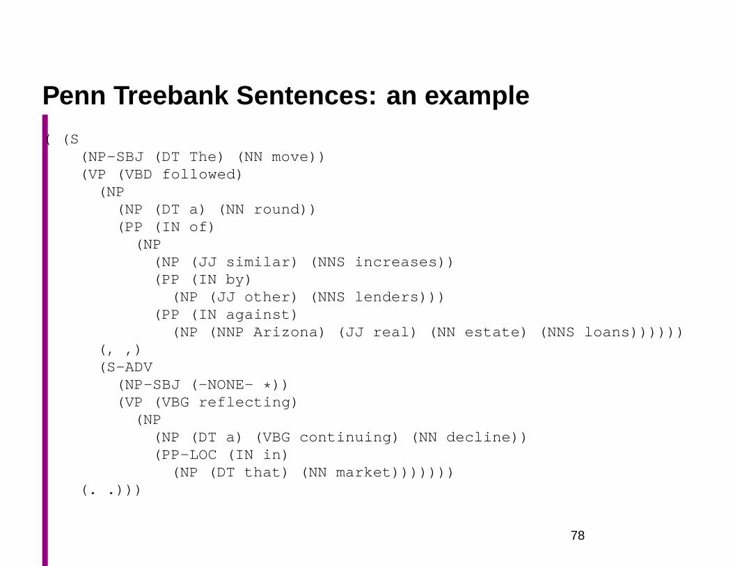
Penn Treebank Sentences: an example( (S
(NP-SBJ (DT The) (NN move))(VP (VBD followed)
(NP(NP (DT a) (NN round))(PP (IN of)
(NP(NP (JJ similar) (NNS increases))(PP (IN by)
(NP (JJ other) (NNS lenders)))(PP (IN against)
(NP (NNP Arizona) (JJ real) (NN estate) (NNS loans))))))(, ,)(S-ADV
(NP-SBJ (-NONE- * ))(VP (VBG reflecting)
(NP(NP (DT a) (VBG continuing) (NN decline))(PP-LOC (IN in)
(NP (DT that) (NN market)))))))(. .)))
78
Ambiguity
• Programming language parsers resolve local ambigui-
ties with lookahead
• Natural languages have global ambiguities:
– I saw that gasoline can explode
• What is the size of embedded NP?
79
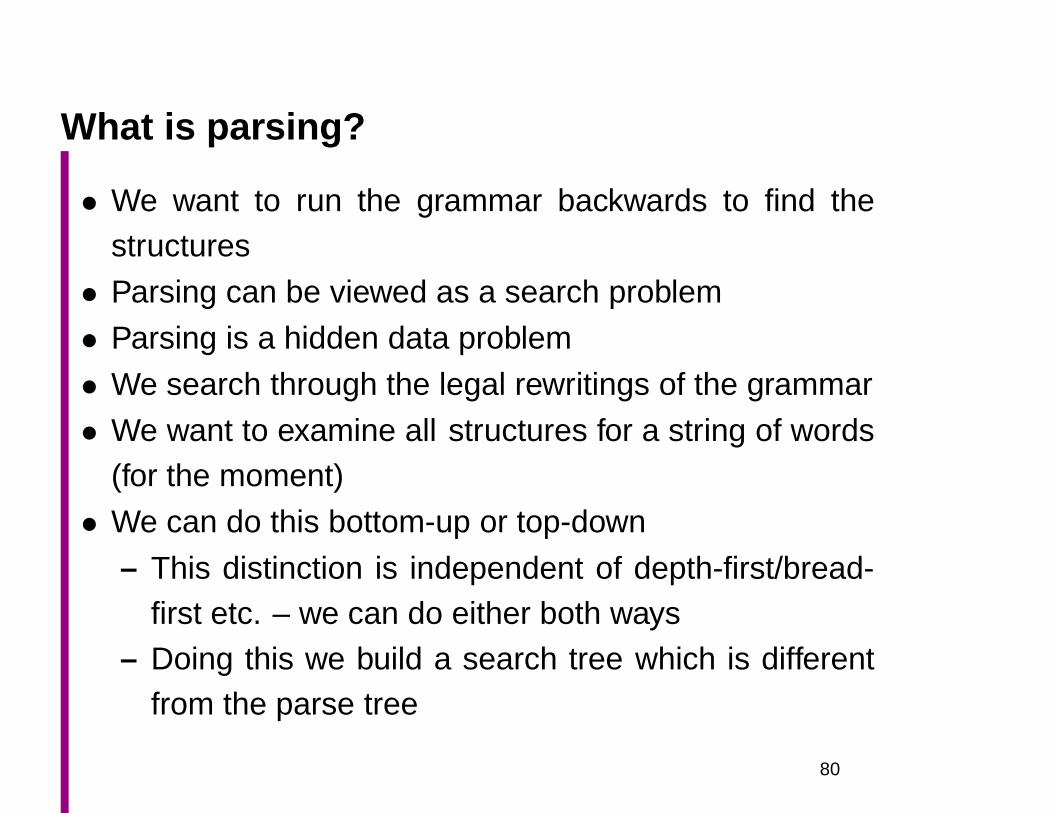
What is parsing?
• We want to run the grammar backwards to find thestructures
• Parsing can be viewed as a search problem
• Parsing is a hidden data problem
• We search through the legal rewritings of the grammar
• We want to examine all structures for a string of words(for the moment)
• We can do this bottom-up or top-down
– This distinction is independent of depth-first/bread-first etc. – we can do either both ways
– Doing this we build a search tree which is differentfrom the parse tree
80
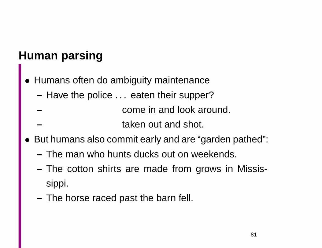
Human parsing
• Humans often do ambiguity maintenance
– Have the police . . . eaten their supper?
– come in and look around.
– taken out and shot.
• But humans also commit early and are “garden pathed”:
– The man who hunts ducks out on weekends.
– The cotton shirts are made from grows in Missis-
sippi.
– The horse raced past the barn fell.
81
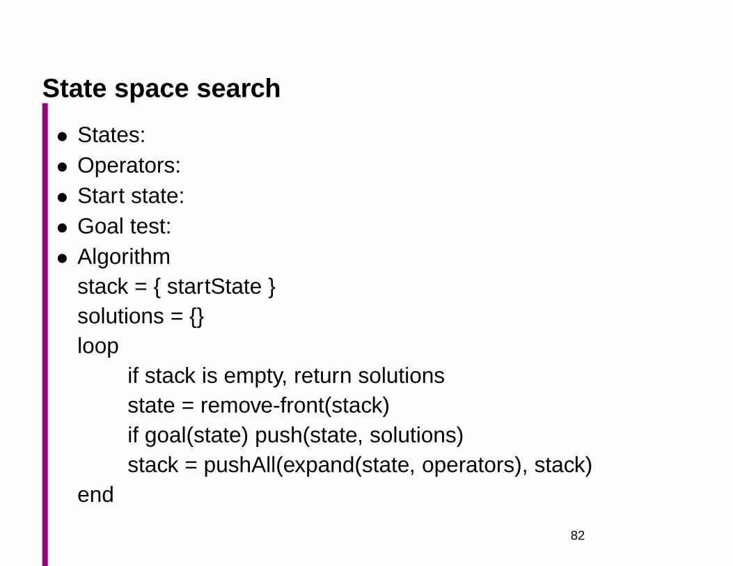
State space search
• States:• Operators:• Start state:• Goal test:• Algorithm
stack = startState solutions = loop
if stack is empty, return solutionsstate = remove-front(stack)if goal(state) push(state, solutions)stack = pushAll(expand(state, operators), stack)
end
82
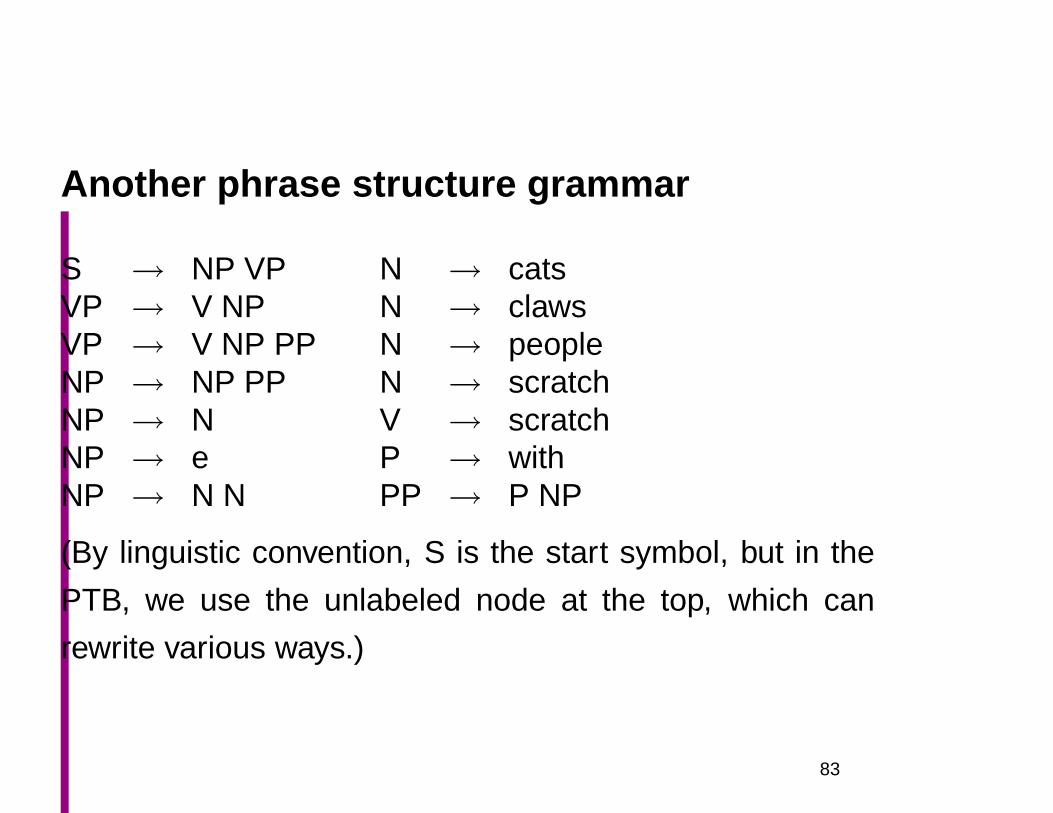
Another phrase structure grammar
S → NP VP N → catsVP → V NP N → clawsVP → V NP PP N → peopleNP → NP PP N → scratchNP → N V → scratchNP → e P → withNP → N N PP → P NP
(By linguistic convention, S is the start symbol, but in the
PTB, we use the unlabeled node at the top, which can
rewrite various ways.)
83

cats scratch people with claws
SNP VPNP PP VP 3 choicesNP PP PP VPoops!N VPcats VPcats V NP 2 choicescats scratch NPcats scratch N 3 choices – showing 2ndcats scratch people oops!cats scratch NP PPcats scratch N PP 3 choices – showing 2nd . . .cats scratch people with claws
84
Phrase Structure (CF) Grammars
G = 〈T,N, S,R〉• T is set of terminals
• N is set of nonterminals
– For NLP, we usually distinguish out a set P ⊂ N of
preterminals which always rewrite as terminals
• S is start symbol (one of the nonterminals)
• R is rules/productions of the form X → γ, where X
is a nonterminal and γ is a sequence of terminals and
nonterminals (may be empty)
• A grammar G generates a language L
85
Recognizers and parsers
• A recognizer is a program for which a given grammar
and a given sentence returns yes if the sentence is
accepted by the grammar (i.e., the sentence is in the
language) and no otherwise
• A parser in addition to doing the work of a recognizer
also returns the set of parse trees for the string
86
Soundness and completeness
• A parser is sound if every parse it returns is valid/correct
• A parser terminates if it is guaranteed to not go off into
an infinite loop
• A parser is complete if for any given grammar and sen-
tence it is sound, produces every valid parse for that
sentence, and terminates
• (For many purposes, we settle for sound but incomplete
parsers: e.g., probabilistic parsers that return a k-best
list)
87
Top-down parsing
• Top-down parsing is goal directed
• A top-down parser starts with a list of constituents to be
built. The top-down parser rewrites the goals in the goal
list by matching one against the LHS of the grammar
rules, and expanding it with the RHS, attempting to
match the sentence to be derived.
• If a goal can be rewritten in several ways, then there is
a choice of which rule to apply (search problem)
• Can use depth-first or breadth-first search, and goal
ordering.
88
Bottom-up parsing
• Bottom-up parsing is data directed
• The initial goal list of a bottom-up parser is the string tobe parsed. If a sequence in the goal list matches theRHS of a rule, then this sequence may be replaced bythe LHS of the rule.
• Parsing is finished when the goal list contains just thestart category.
• If the RHS of several rules match the goal list, thenthere is a choice of which rule to apply (search problem)
• Can use depth-first or breadth-first search, and goalordering.
• The standard presentation is as shift-reduce parsing.
89
Problems with top-down parsing
• Left recursive rules
• A top-down parser will do badly if there are many differ-ent rules for the same LHS. Consider if there are 600rules for S, 599 of which start with NP, but one of whichstarts with V, and the sentence starts with V.
• Useless work: expands things that are possible top-down but not there
• Top-down parsers do well if there is useful grammar-driven control: search is directed by the grammar
• Top-down is hopeless for rewriting parts of speech (preter-minals) with words (terminals). In practice that is al-ways done bottom-up as lexical lookup.
90

1
• Repeated work: anywhere there is common substruc-
ture
Problems with bottom-up parsing
• Unable to deal with empty categories: termination prob-lem, unless rewriting empties as constituents is some-how restricted (but then it’s generally incomplete)• Useless work: locally possible, but globally impossible.• Inefficient when there is great lexical ambiguity (grammar-
driven control might help here)• Conversely, it is data-directed: it attempts to parse the
words that are there.• Repeated work: anywhere there is common substruc-
ture• Both TD (LL) and BU (LR) parsers can (and frequently
do) do work exponential in the sentence length on NLPproblems.
91
Principles for success: what one needs to do
• If you are going to do parsing-as-search with a gram-
mar as is:
– Left recursive structures must be found, not predicted
– Empty categories must be predicted, not found
• Doing these things doesn’t fix the repeated work prob-
lem.
92
An alternative way to fix things
• Grammar transformations can fix both left-recursion and
epsilon productions
• Then you parse the same language but with different
trees
• Linguists tend to hate you
– But this is a misconception: they shouldn’t
– You can fix the trees post hoc
93
A second way to fix things
• Rather than doing parsing-as-search, we do parsing as
dynamic programming
• This is the most standard way to do things
• It solves the problem of doing repeated work
• But there are also other ways of solving the problem of
doing repeated work
– Memoization (remembering solved subproblems)
– Doing graph-search rather than tree-search.
94
Filtering
• Conversion to CNF. First remove ǫ categories.
• Directed vs. Undirected parsers: using the opposite
direction for x filtering.
95
Left corner parsing
• Left corner parsing: Accept word. What is it left-corner
of? Parse that constituent top down. Can prune on
top-down knowledge. Doesn’t have problem with left
recursion except with unaries. Does have problem with
empties in left corner, but not while working top down.
96
n-gram models and statisticalestimation
FSNLP, chapter 6
Christopher Manning andHinrich Schütze
© 1999–200297
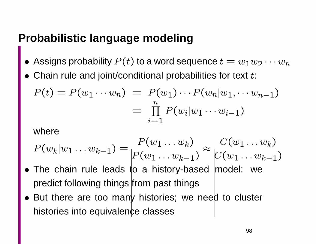
Probabilistic language modeling
• Assigns probability P (t) to a word sequence t = w1w2 · · ·wn• Chain rule and joint/conditional probabilities for text t:
P (t) = P (w1 · · ·wn) = P (w1) · · ·P (wn|w1, · · ·wn−1)
=n∏
i=1P (wi|w1 · · ·wi−1)
where
P (wk|w1 . . . wk−1) =P (w1 . . . wk)
P (w1 . . . wk−1)≈ C(w1 . . . wk)
C(w1 . . . wk−1)
• The chain rule leads to a history-based model: we
predict following things from past things
• But there are too many histories; we need to cluster
histories into equivalence classes
98
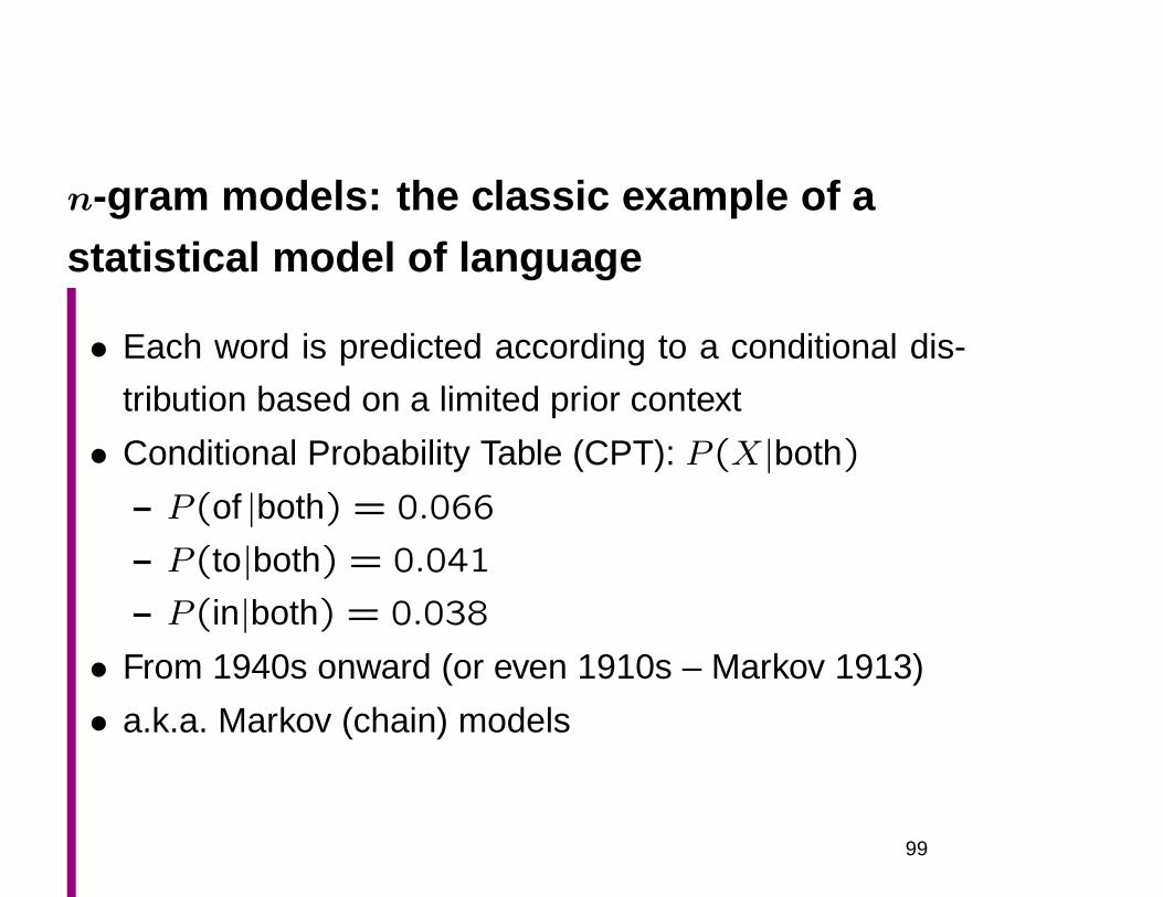
n-gram models: the classic example of astatistical model of language
• Each word is predicted according to a conditional dis-
tribution based on a limited prior context
• Conditional Probability Table (CPT): P (X|both)
– P (of |both) = 0.066
– P (to|both) = 0.041
– P (in|both) = 0.038
• From 1940s onward (or even 1910s – Markov 1913)
• a.k.a. Markov (chain) models
99
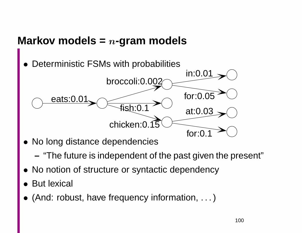
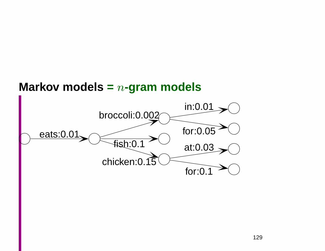
Markov models = n-gram models
• Deterministic FSMs with probabilities
eats:0.01
broccoli:0.002in:0.01
for:0.05fish:0.1
chicken:0.15
at:0.03
for:0.1• No long distance dependencies
– “The future is independent of the past given the present”
• No notion of structure or syntactic dependency
• But lexical
• (And: robust, have frequency information, . . . )
100
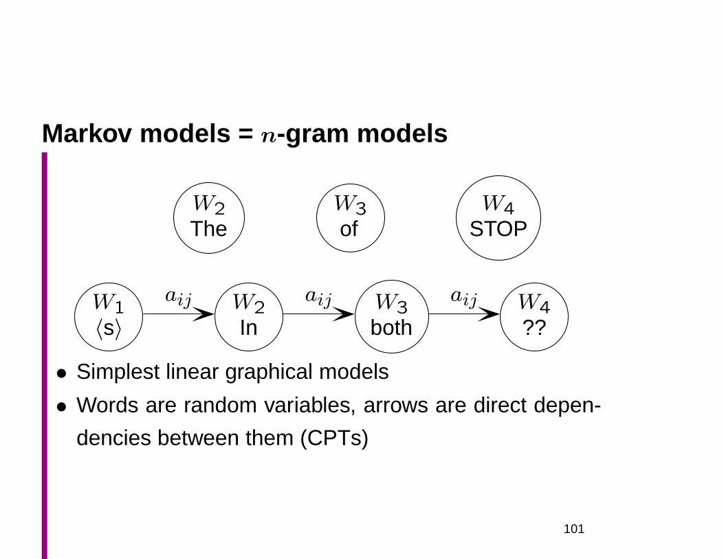
Markov models = n-gram models
W2The
W3of
W4STOP
W1〈s〉
W2In
W3both
W4??
aij aij aij
• Simplest linear graphical models
• Words are random variables, arrows are direct depen-
dencies between them (CPTs)
101
n-gram models
• Core language model for the engineering task of better
predicting the next word:
– Speech recognition
– OCR
– Context-sensitive spelling correction
• These simple engineering models have just been amaz-
ingly successful.
• It is only recently that they have been improved on for
these tasks (Chelba and Jelinek 1998; Charniak 2001).
• But linguistically, they are appalling simple and naive
102
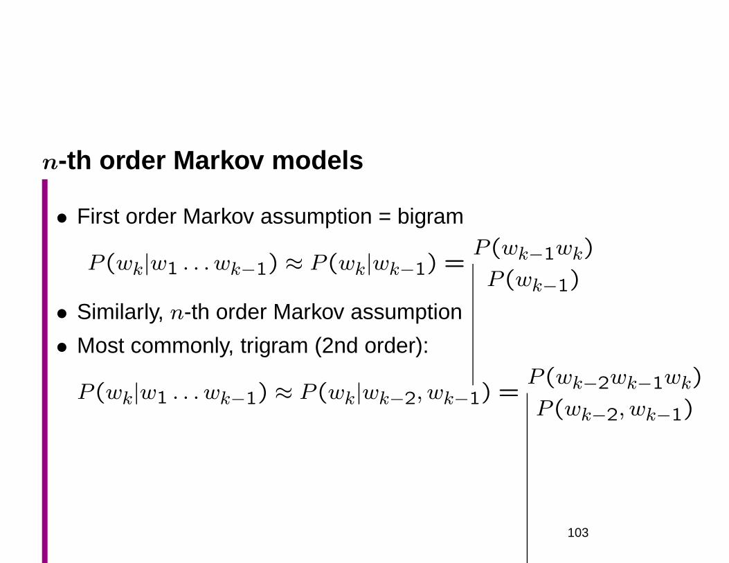
n-th order Markov models
• First order Markov assumption = bigram
P (wk|w1 . . . wk−1) ≈ P (wk|wk−1) =P (wk−1wk)
P (wk−1)
• Similarly, n-th order Markov assumption
• Most commonly, trigram (2nd order):
P (wk|w1 . . . wk−1) ≈ P (wk|wk−2, wk−1) =P (wk−2wk−1wk)
P (wk−2, wk−1)
103
Why mightn’t n-gram models work?
• Relationships (say between subject and verb) can be
arbitrarily distant and convoluted, as linguists love to
point out:
– The man that I was watching without pausing to look
at what was happening down the street, and quite
oblivious to the situation that was about to befall him
confidently strode into the center of the road.
104
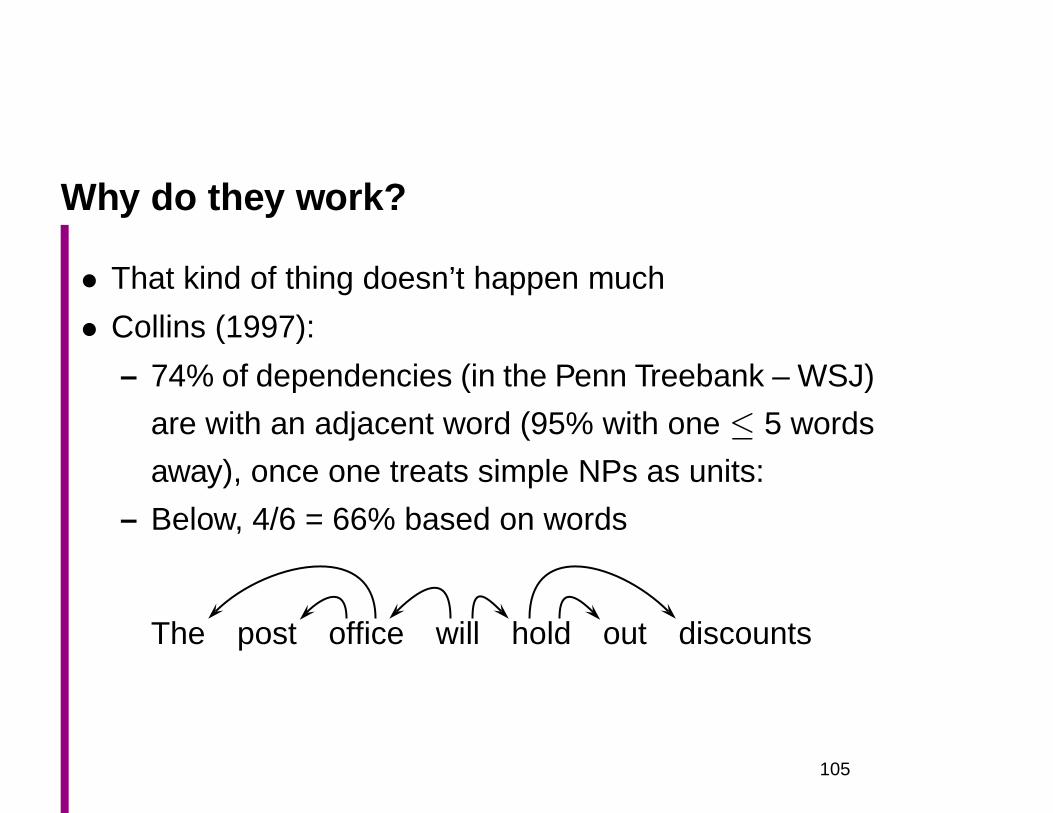
Why do they work?
• That kind of thing doesn’t happen much
• Collins (1997):
– 74% of dependencies (in the Penn Treebank – WSJ)
are with an adjacent word (95% with one ≤ 5 words
away), once one treats simple NPs as units:
– Below, 4/6 = 66% based on words
The post office will hold out discounts
105
Why is that?
Sapir (1921: 14):
‘When I say, for instance, “I had a good breakfast
this morning,” it is clear that I am not in the throes
of laborious thought, that what I have to transmit
is hardly more than a pleasurable memory symbol-
ically rendered in the grooves of habitual expres-
sion. . . . It is somewhat as though a dynamo capa-
ble of generating enough power to run an elevator
were operated almost exclusively to feed an electric
doorbell.’
106
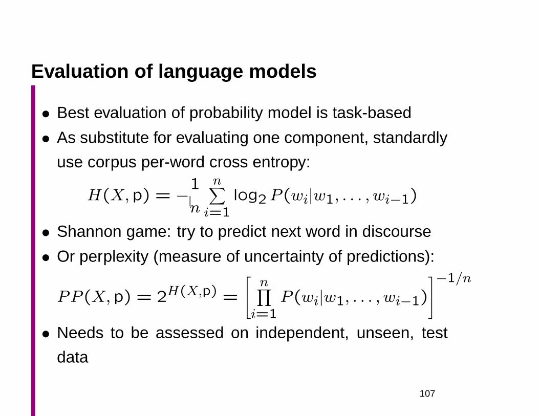
Evaluation of language models
• Best evaluation of probability model is task-based
• As substitute for evaluating one component, standardly
use corpus per-word cross entropy:
H(X,p) = −1
n
n∑
i=1log2P (wi|w1, . . . , wi−1)
• Shannon game: try to predict next word in discourse
• Or perplexity (measure of uncertainty of predictions):
PP (X,p) = 2H(X,p) =
n∏
i=1P (wi|w1, . . . , wi−1)
−1/n
• Needs to be assessed on independent, unseen, test
data
107
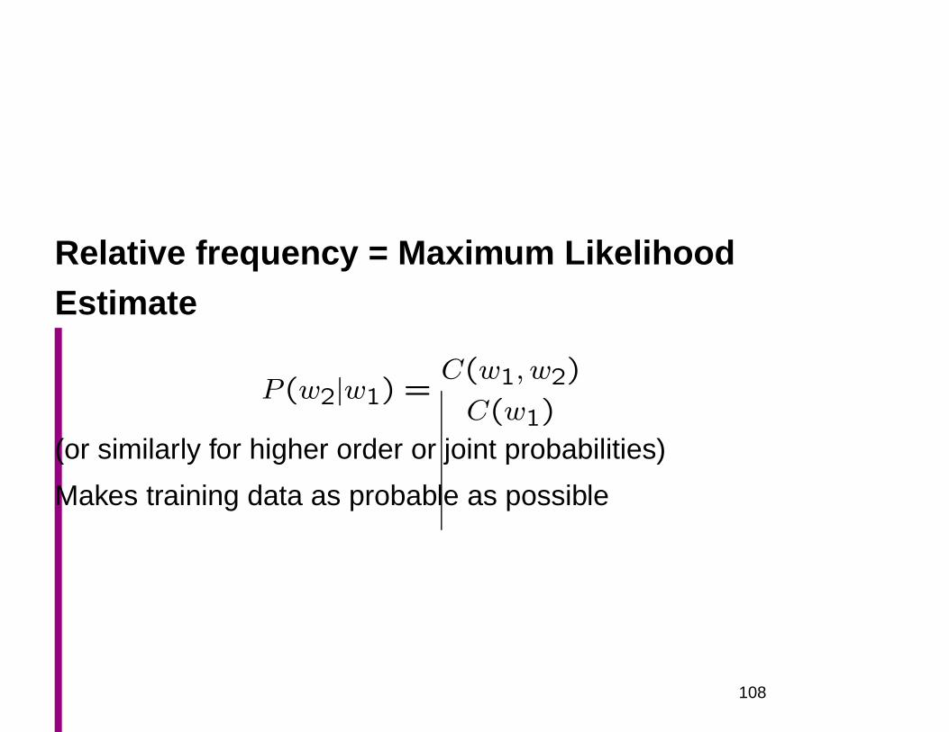
Relative frequency = Maximum LikelihoodEstimate
P (w2|w1) =C(w1, w2)
C(w1)
(or similarly for higher order or joint probabilities)
Makes training data as probable as possible
108
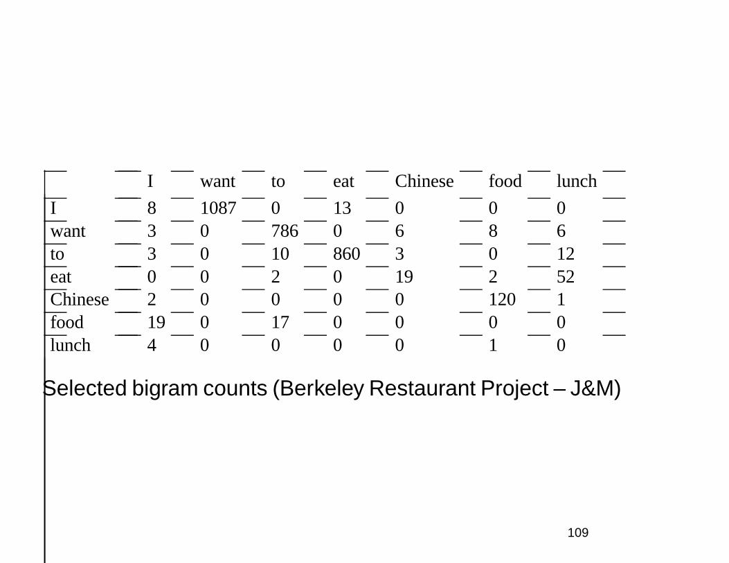
I want to eat Chinese food lunch
I 8 1087 0 13 0 0 0want 3 0 786 0 6 8 6to 3 0 10 860 3 0 12eat 0 0 2 0 19 2 52Chinese 2 0 0 0 0 120 1food 19 0 17 0 0 0 0lunch 4 0 0 0 0 1 0
Selected bigram counts (Berkeley Restaurant Project – J&M)
109
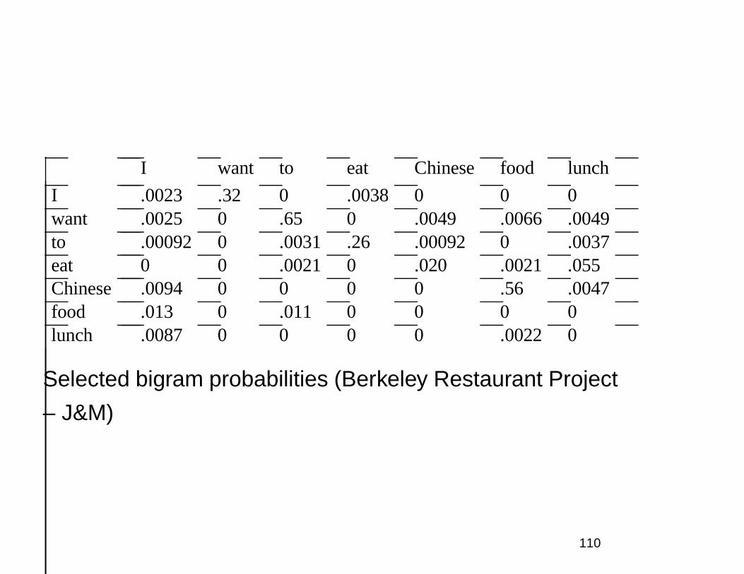
I want to eat Chinese food lunch
I .0023 .32 0 .0038 0 0 0want .0025 0 .65 0 .0049 .0066 .0049to .00092 0 .0031 .26 .00092 0 .0037eat 0 0 .0021 0 .020 .0021 .055Chinese .0094 0 0 0 0 .56 .0047food .013 0 .011 0 0 0 0lunch .0087 0 0 0 0 .0022 0
Selected bigram probabilities (Berkeley Restaurant Project
– J&M)
110
Limitations of Maximum Likelihood Estimator
Problem: We are often infinitely surprised when unseen
word appears (P (unseen) = 0)
• Problem: this happens commonly.
• Probabilities of zero count words are too low
• Probabilities of nonzero count words are too high
• Estimates for high count words are fairly accurate
• Estimates for low count words are mostly inaccurate
• We need smoothing! (We flatten spiky distribution and
give shavings to unseen items.)
111
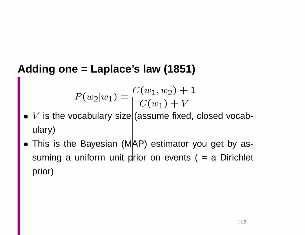
Adding one = Laplace’s law (1851)
P (w2|w1) =C(w1, w2) + 1
C(w1) + V
• V is the vocabulary size (assume fixed, closed vocab-
ulary)
• This is the Bayesian (MAP) estimator you get by as-
suming a uniform unit prior on events ( = a Dirichlet
prior)
112
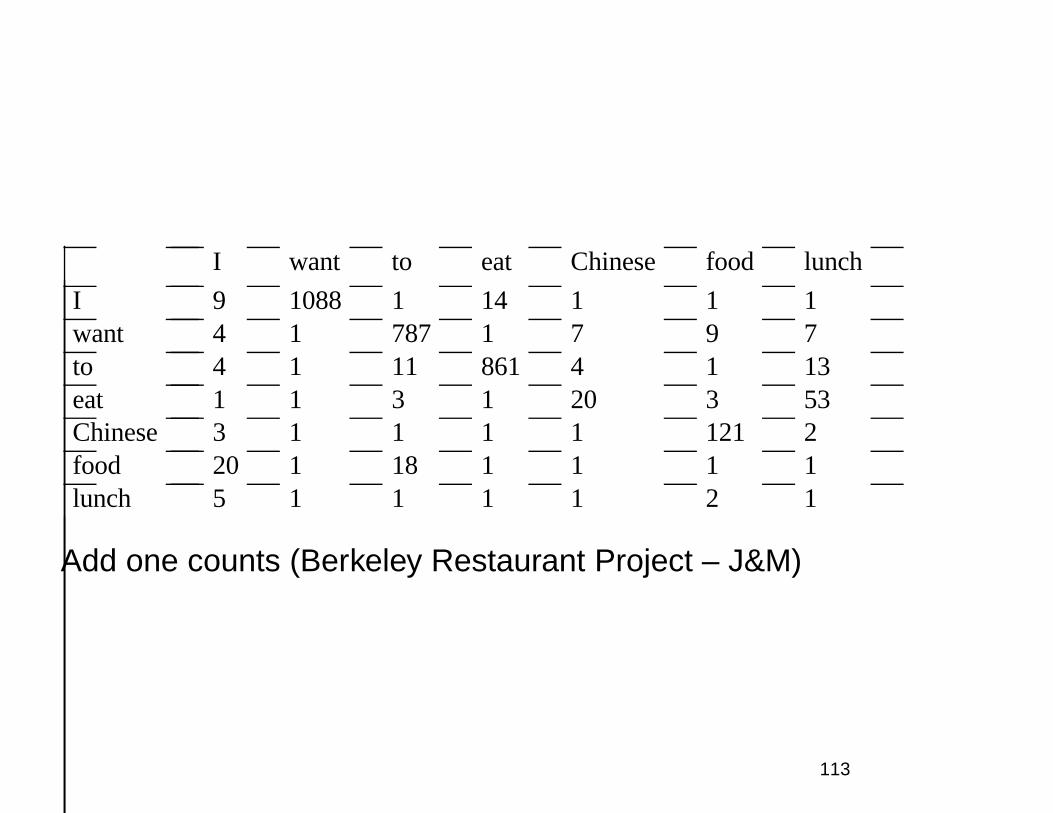
I want to eat Chinese food lunch
I 9 1088 1 14 1 1 1want 4 1 787 1 7 9 7to 4 1 11 861 4 1 13eat 1 1 3 1 20 3 53Chinese 3 1 1 1 1 121 2food 20 1 18 1 1 1 1lunch 5 1 1 1 1 2 1
Add one counts (Berkeley Restaurant Project – J&M)
113
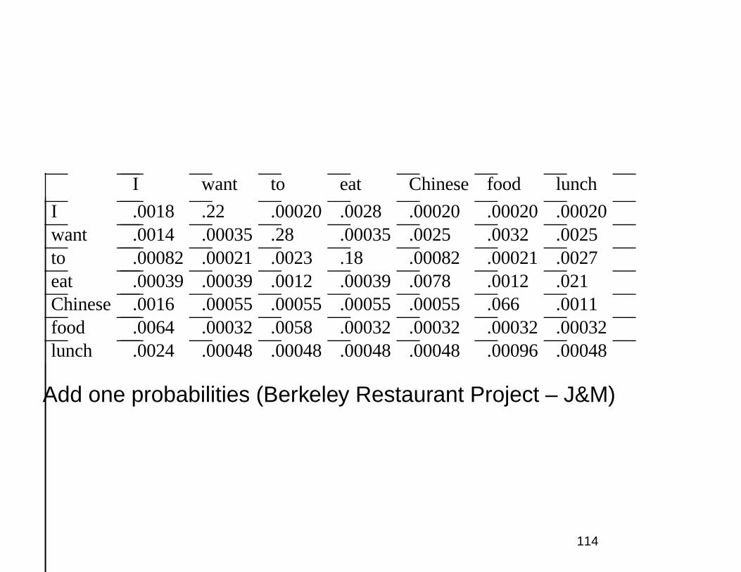
I want to eat Chinese food lunch
I .0018 .22 .00020 .0028 .00020 .00020 .00020want .0014 .00035 .28 .00035 .0025 .0032 .0025to .00082 .00021 .0023 .18 .00082 .00021 .0027eat .00039 .00039 .0012 .00039 .0078 .0012 .021Chinese .0016 .00055 .00055 .00055 .00055 .066 .0011food .0064 .00032 .0058 .00032 .00032 .00032 .00032lunch .0024 .00048 .00048 .00048 .00048 .00096 .00048
Add one probabilities (Berkeley Restaurant Project – J&M)
114
I want to eat Chinese food lunch
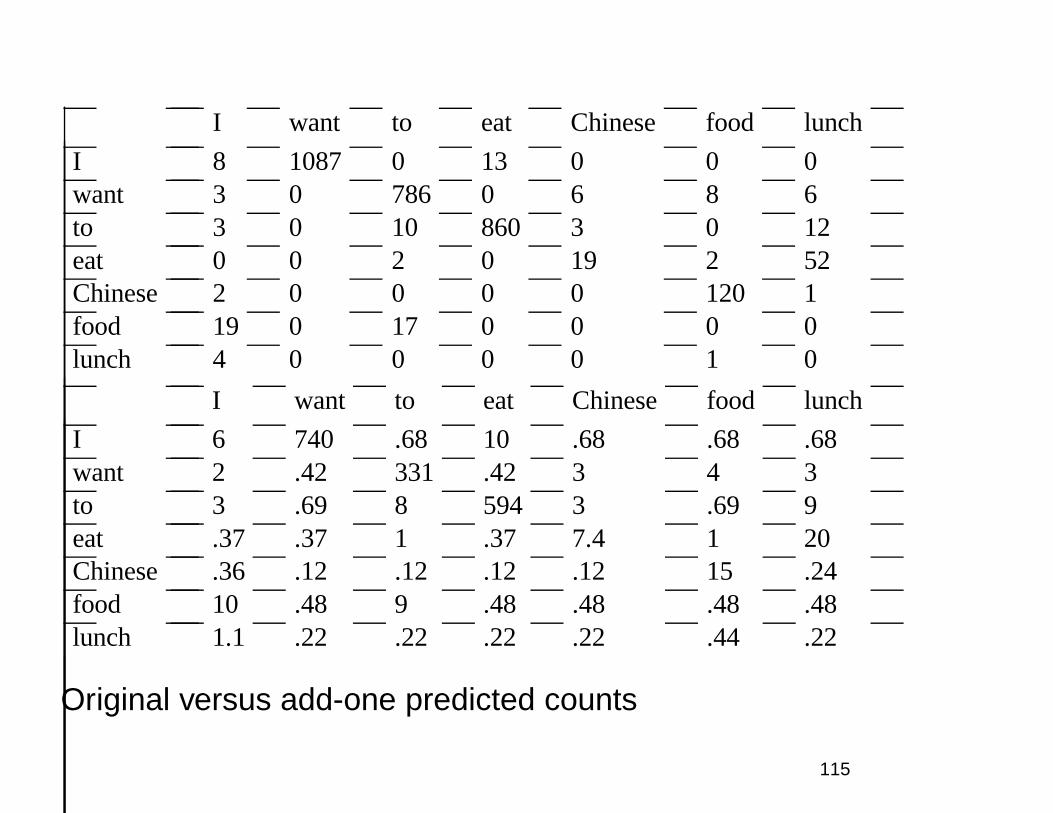
I 8 1087 0 13 0 0 0want 3 0 786 0 6 8 6to 3 0 10 860 3 0 12eat 0 0 2 0 19 2 52Chinese 2 0 0 0 0 120 1food 19 0 17 0 0 0 0lunch 4 0 0 0 0 1 0
I want to eat Chinese food lunch
I 6 740 .68 10 .68 .68 .68want 2 .42 331 .42 3 4 3to 3 .69 8 594 3 .69 9eat .37 .37 1 .37 7.4 1 20Chinese .36 .12 .12 .12 .12 15 .24food 10 .48 9 .48 .48 .48 .48lunch 1.1 .22 .22 .22 .22 .44 .22
Original versus add-one predicted counts
115
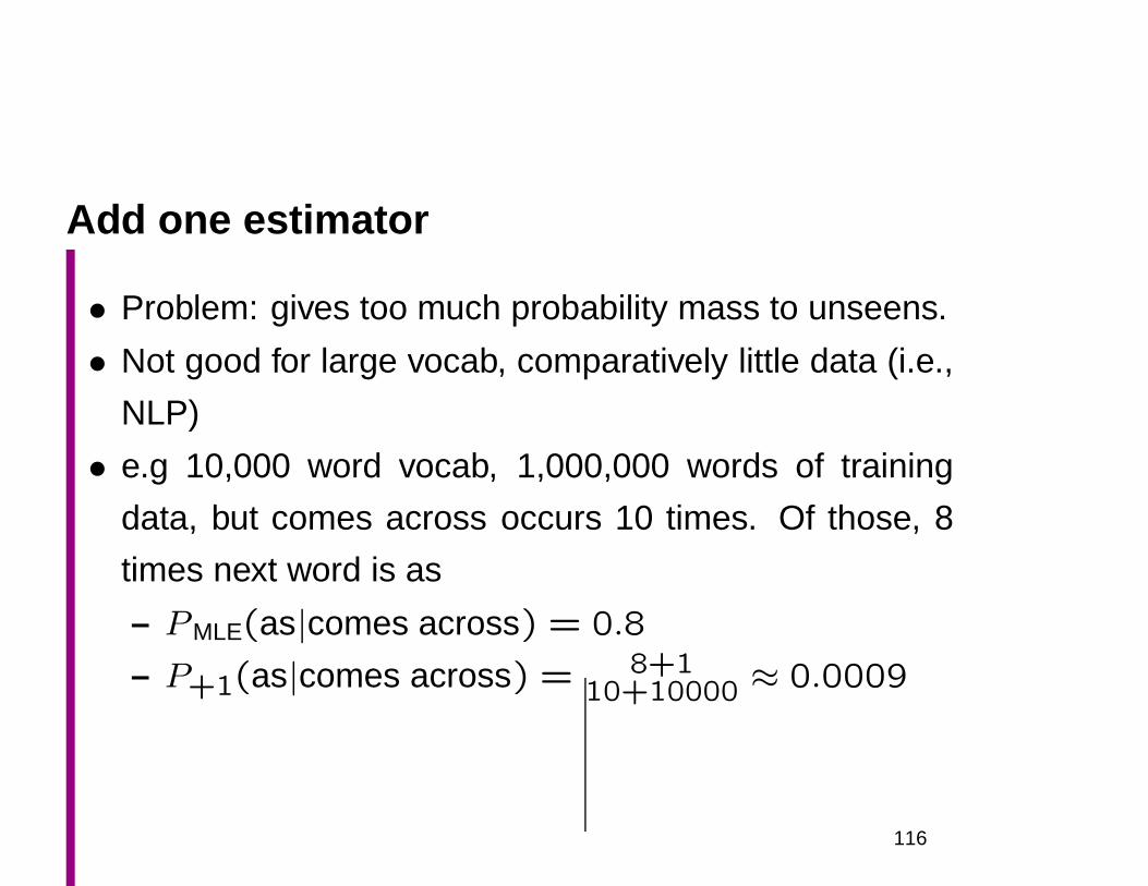
Add one estimator
• Problem: gives too much probability mass to unseens.
• Not good for large vocab, comparatively little data (i.e.,
NLP)
• e.g 10,000 word vocab, 1,000,000 words of training
data, but comes across occurs 10 times. Of those, 8
times next word is as
– PMLE(as|comes across) = 0.8
– P+1(as|comes across) = 8+110+10000 ≈ 0.0009
116
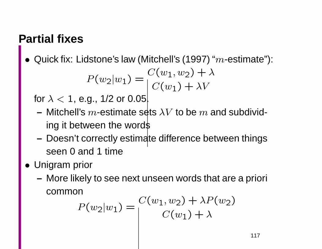
Partial fixes
• Quick fix: Lidstone’s law (Mitchell’s (1997) “m-estimate”):
P (w2|w1) =C(w1, w2) + λ
C(w1) + λV
for λ < 1, e.g., 1/2 or 0.05.– Mitchell’sm-estimate sets λV to bem and subdivid-
ing it between the words– Doesn’t correctly estimate difference between things
seen 0 and 1 time• Unigram prior
– More likely to see next unseen words that are a prioricommon
P (w2|w1) =C(w1, w2) + λP (w2)
C(w1) + λ
117
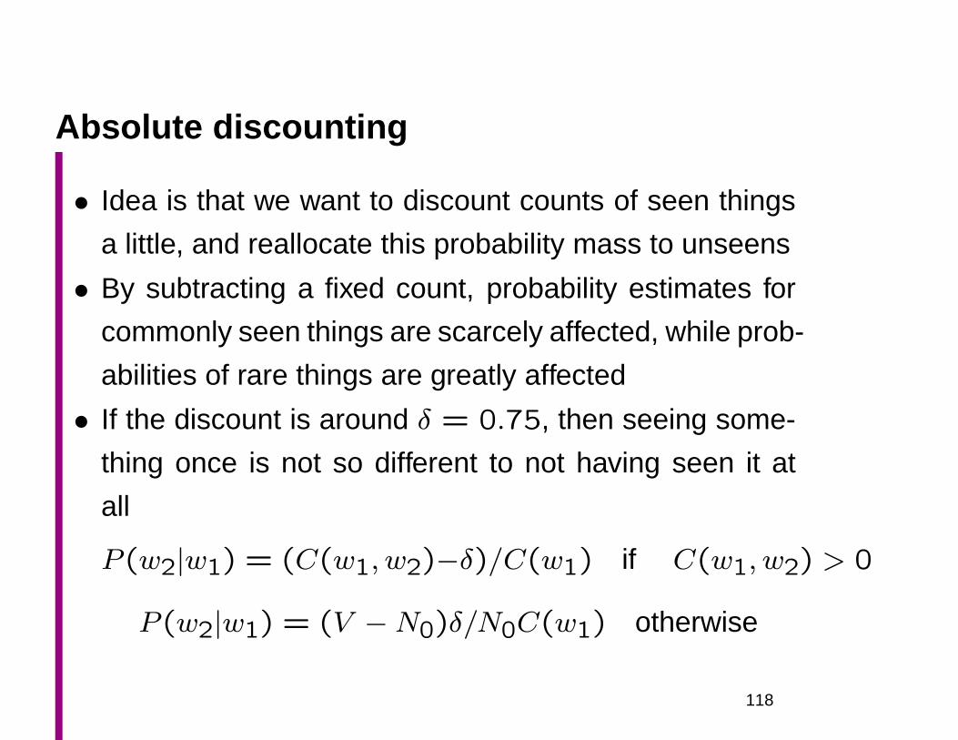
Absolute discounting
• Idea is that we want to discount counts of seen things
a little, and reallocate this probability mass to unseens
• By subtracting a fixed count, probability estimates for
commonly seen things are scarcely affected, while prob-
abilities of rare things are greatly affected
• If the discount is around δ = 0.75, then seeing some-
thing once is not so different to not having seen it at
all
P (w2|w1) = (C(w1, w2)−δ)/C(w1) if C(w1, w2) > 0
P (w2|w1) = (V −N0)δ/N0C(w1) otherwise
118
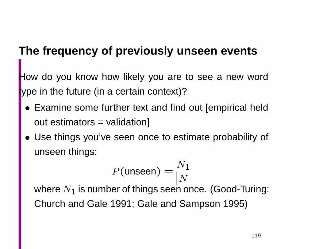
The frequency of previously unseen events
How do you know how likely you are to see a new word
type in the future (in a certain context)?
• Examine some further text and find out [empirical held
out estimators = validation]
• Use things you’ve seen once to estimate probability of
unseen things:
P (unseen) =N1
NwhereN1 is number of things seen once. (Good-Turing:
Church and Gale 1991; Gale and Sampson 1995)
119
Good-Turing smoothing
Derivation reflects leave-one out estimation (Ney et al. 1997):
• For each word token in data, call it the test set; remain-
ing data is training set
• See how often word in test set has r counts in training
set
• This will happen every time word left out has r + 1
counts in original data
• So total count mass of r count words is assigned from
mass of r+ 1 count words [= Nr+1 × (r+ 1)]
• Doesn’t require held out data (which is good!)
120
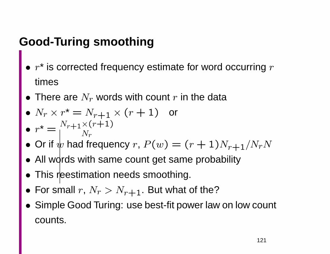
Good-Turing smoothing
• r* is corrected frequency estimate for word occurring r
times
• There are Nr words with count r in the data
• Nr × r* = Nr+1 × (r+ 1) or
• r* =Nr+1×(r+1)
Nr
• Or if w had frequency r, P (w) = (r+ 1)Nr+1/NrN
• All words with same count get same probability
• This reestimation needs smoothing.
• For small r, Nr > Nr+1. But what of the?
• Simple Good Turing: use best-fit power law on low count
counts.
121
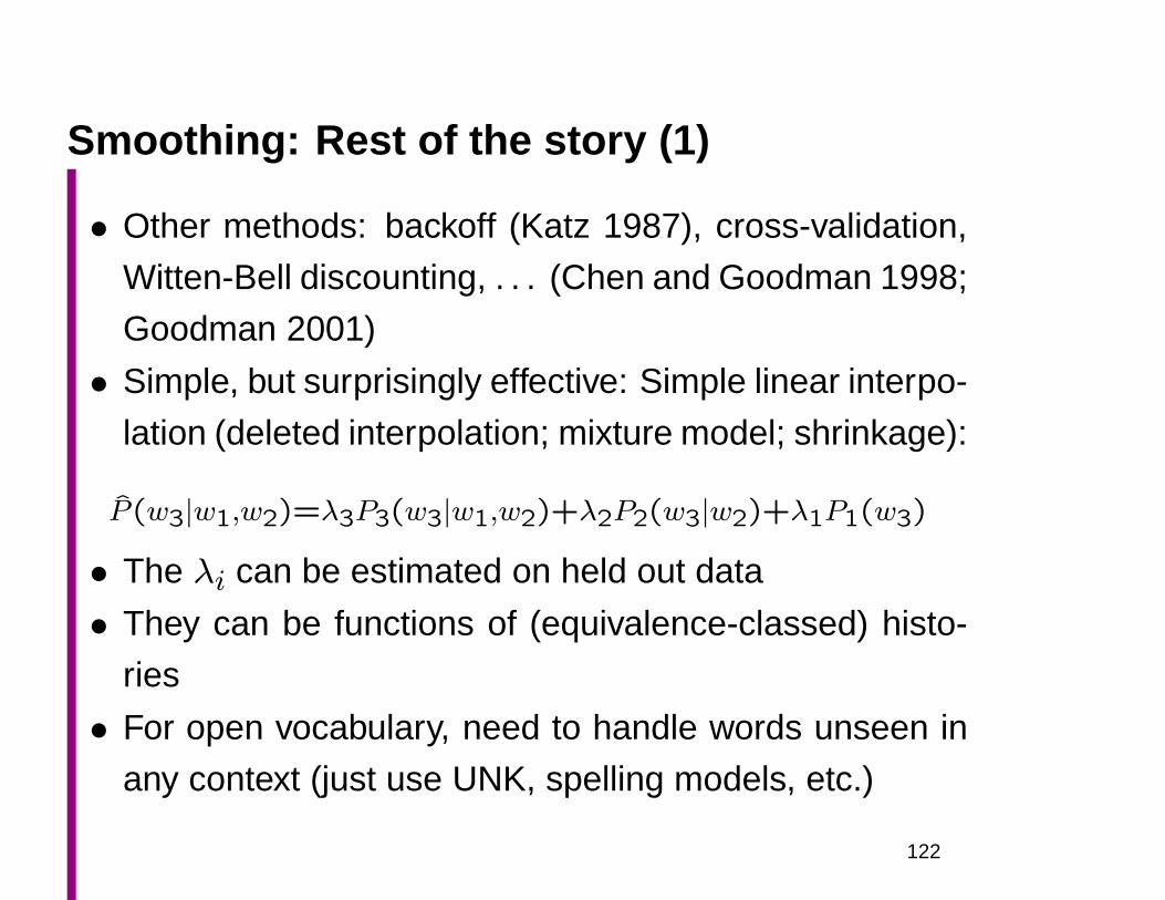
Smoothing: Rest of the story (1)
• Other methods: backoff (Katz 1987), cross-validation,
Witten-Bell discounting, . . . (Chen and Goodman 1998;
Goodman 2001)
• Simple, but surprisingly effective: Simple linear interpo-
lation (deleted interpolation; mixture model; shrinkage):
P(w3|w1,w2)=λ3P3(w3|w1,w2)+λ2P2(w3|w2)+λ1P1(w3)
• The λi can be estimated on held out data
• They can be functions of (equivalence-classed) histo-
ries
• For open vocabulary, need to handle words unseen in
any context (just use UNK, spelling models, etc.)
122
Smoothing: Rest of the story (2)
• Recent work emphasizes constraints on the smoothed
model
• Kneser and Ney (1995): Backoff n-gram counts not
proportional to frequency of n-gram in training data but
to expectation of how often it should occur in novel
trigram – since one only uses backoff estimate when
trigram not found
• (Smoothed) maximum entropy (a.k.a. loglinear) models
again place constraints on the distribution (Rosenfeld
1996, 2000)
123
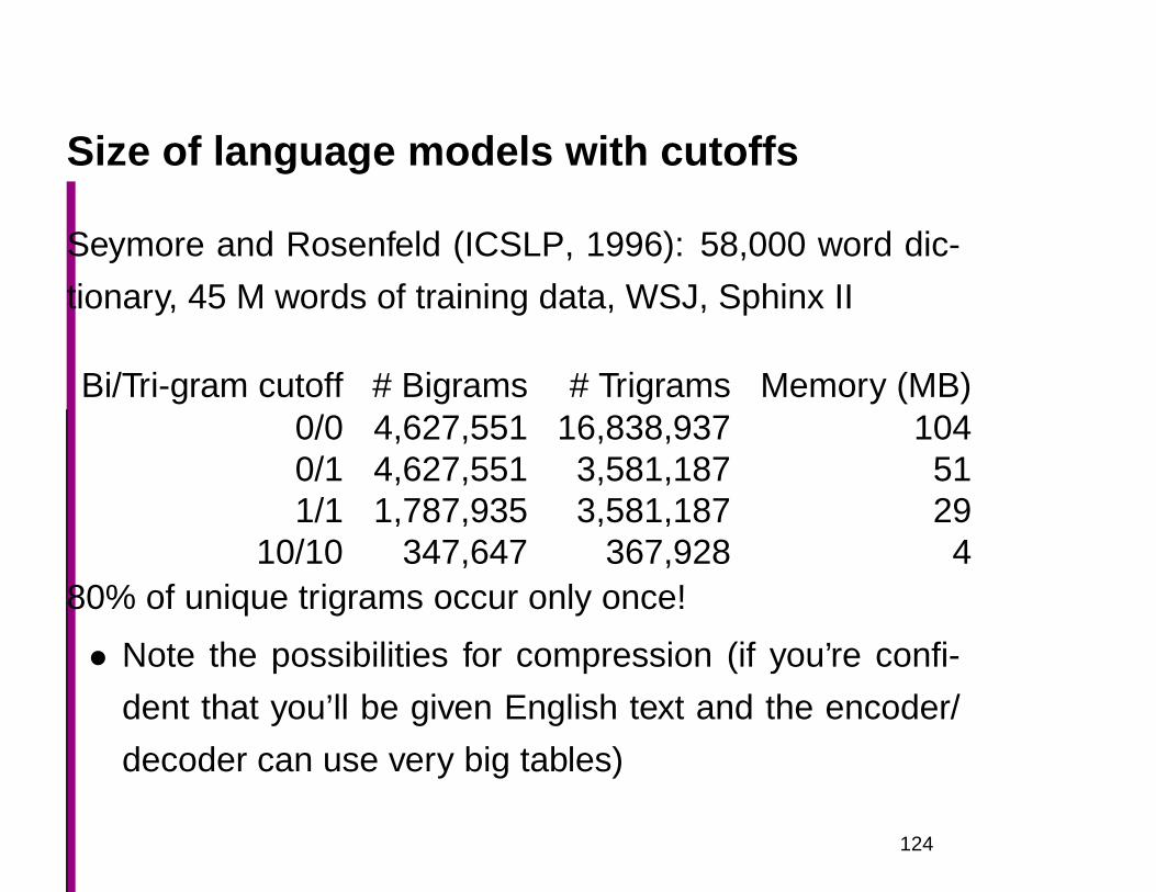
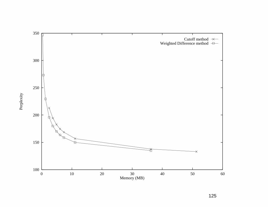
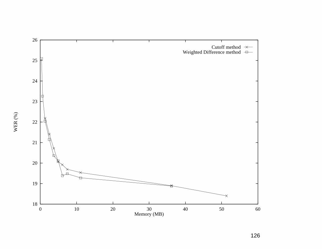
Size of language models with cutoffs
Seymore and Rosenfeld (ICSLP, 1996): 58,000 word dic-
tionary, 45 M words of training data, WSJ, Sphinx II
Bi/Tri-gram cutoff # Bigrams # Trigrams Memory (MB)0/0 4,627,551 16,838,937 1040/1 4,627,551 3,581,187 511/1 1,787,935 3,581,187 29
10/10 347,647 367,928 480% of unique trigrams occur only once!
• Note the possibilities for compression (if you’re confi-
dent that you’ll be given English text and the encoder/
decoder can use very big tables)
124
100
150
200
250
300
350
0 10 20 30 40 50 60
Per
plex
ity
Memory (MB)
Cutoff methodWeighted Difference method
125
18
19
20
21
22
23
24
25
26
0 10 20 30 40 50 60
WE
R (
%)
Memory (MB)
Cutoff methodWeighted Difference method
126
More LM facts
• Seymore, Chen, Eskenazi and Rosenfeld (1996)
• HUB-4: Broadcast News 51,000 word vocab, 130M words
training. Katz backoff smoothing (1/1 cutoff).
• Perplexity 231
• 0/0 cutoff: 3% perplexity reduction
• 7-grams: 15% perplexity reduction
• Note the possibilities for compression, if you’re confi-
dent that you’ll be given English text (and the encoder/
decoder can use very big tables)
127

Extra slides
128
Markov models = n-gram models
eats:0.01
broccoli:0.002in:0.01
for:0.05fish:0.1
chicken:0.15
at:0.03
for:0.1
129
Markov models
• Deterministic FSMs with probabilities
• No long distance dependencies
– “The future is independent of the past given the present”
• No notion of structure or syntactic dependency
• But lexical
• (And: robust, have frequency information, . . . )
130
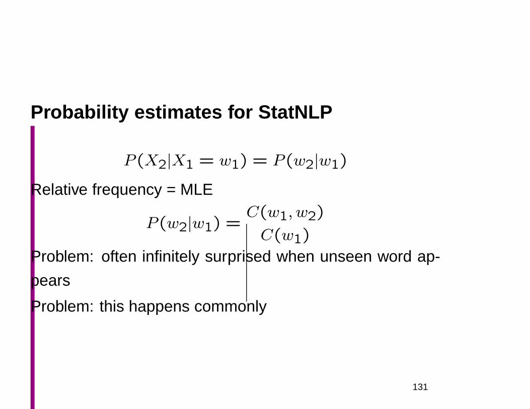
Probability estimates for StatNLP
P (X2|X1 = w1) = P (w2|w1)
Relative frequency = MLE
P (w2|w1) =C(w1, w2)
C(w1)
Problem: often infinitely surprised when unseen word ap-
pears
Problem: this happens commonly
131
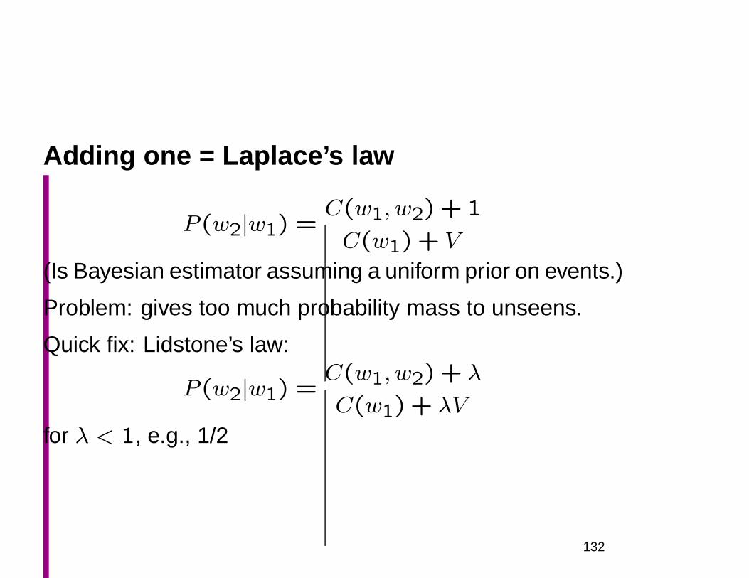
Adding one = Laplace’s law
P (w2|w1) =C(w1, w2) + 1
C(w1) + V
(Is Bayesian estimator assuming a uniform prior on events.)
Problem: gives too much probability mass to unseens.
Quick fix: Lidstone’s law:
P (w2|w1) =C(w1, w2) + λ
C(w1) + λV
for λ < 1, e.g., 1/2
132
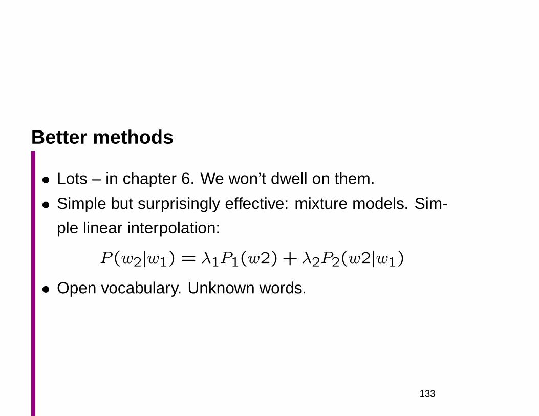
Better methods
• Lots – in chapter 6. We won’t dwell on them.
• Simple but surprisingly effective: mixture models. Sim-
ple linear interpolation:
P (w2|w1) = λ1P1(w2) + λ2P2(w2|w1)
• Open vocabulary. Unknown words.
133
Managing data
• Training data
• Validation data
• Final testing data
• Cross-validation
– One score doesn’t allow system comparison
– This allows confidence ranges to be computed
– And systems to be compared with confidence!
134
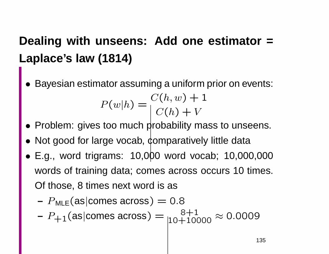
Dealing with unseens: Add one estimator =Laplace’s law (1814)
• Bayesian estimator assuming a uniform prior on events:
P (w|h) =C(h, w) + 1
C(h) + V
• Problem: gives too much probability mass to unseens.
• Not good for large vocab, comparatively little data
• E.g., word trigrams: 10,000 word vocab; 10,000,000
words of training data; comes across occurs 10 times.
Of those, 8 times next word is as
– PMLE(as|comes across) = 0.8
– P+1(as|comes across) = 8+110+10000 ≈ 0.0009
135
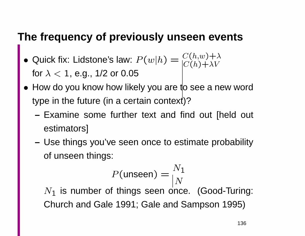
The frequency of previously unseen events
• Quick fix: Lidstone’s law: P (w|h) = C(h,w)+λC(h)+λV
for λ < 1, e.g., 1/2 or 0.05
• How do you know how likely you are to see a new word
type in the future (in a certain context)?
– Examine some further text and find out [held out
estimators]
– Use things you’ve seen once to estimate probability
of unseen things:
P (unseen) =N1
NN1 is number of things seen once. (Good-Turing:
Church and Gale 1991; Gale and Sampson 1995)
136
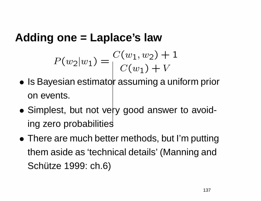
Adding one = Laplace’s law
P(w2|w1) =C(w1, w2) + 1
C(w1) + V
• Is Bayesian estimator assuming a uniform prior
on events.
• Simplest, but not very good answer to avoid-
ing zero probabilities
• There are much better methods, but I’m putting
them aside as ‘technical details’ (Manning and
Schütze 1999: ch.6)
137
Language model topic determination
• Start with some documents labeled for topic (ci)
• Train an n-gram language model just on documents of
each topic, which we regard as a ‘language’
• Testing: Decide which topic/language is most likely to
have generated a new document, by calculating the
P (w1 · · ·wn|ci)• Choose the most probable one as the topic of the doc-
ument
138

Disambiguating using ‘language’ models
• Supervised training from hand-labeled examples
• Train n-gram language model for examples of each sense,
treating examples as a ‘language’
– estimate P (port|sailed, into), etc.
– reduce parameters by backing off where there is in-
sufficient data: P (port|into) or P (port) [unigram es-
timate for sense]
• Disambiguate based on in which ‘language’ the sen-
tence would have highest probability
• This gives some of the advantages of wide context bag
of words models (Naive Bayes-like) and use of local
structural cues around word
139
Word Sense Disambiguation
FSNLP, chapter 7
Christopher Manning andHinrich Schütze
© 1999–2004
140
Word sense disambiguation
• The task is to determine which of various senses of a
word are invoked in context:
– the seed companies cut off the tassels of each plant,
making it male sterile
– Nissan’s Tennessee manufacturing plant beat back
a United Auto Workers organizing effort with aggres-
sive tactics
• This is an important problem: Most words are ambigu-
ous (have multiple senses)
• Converse: words or senses that mean (almost) the same:
image, likeness, portrait, facsimile, picture
141

WSD: Many other cases are harder
• title:
– Name/heading of a book, statute, work of art or mu-
sic, etc.
– Material at the start of a film
– The right of legal ownership (of land)
– The document that is evidence of this right
– An appellation of respect attached to a person’s name
– A written work
142
WSD: The many meanings of interest [n.]
• Readiness to give attention to or to learn about some-
thing
• Quality of causing attention to be given
• Activity, subject, etc., which one gives time and atten-
tion to
• The advantage, advancement or favor of an individual
or group
• A stake or share (in a company, business, etc.)
• Money paid regularly for the use of money
143

WSD: Many other cases are harder• modest:
– In evident apprehension that such a prospect might frighten off the youngor composers of more modest 1 forms –
– Tort reform statutes in thirty-nine states have effected modest 9 changes ofsubstantive and remedial law
– The modest 9 premises are announced with a modest and simple name –– In the year before the Nobel Foundation belatedly honoured this modest 0
and unassuming individual,– LinkWay is IBM’s response to HyperCard, and in Glasgow (its UK launch)
it impressed many by providing colour, by its modest 9 memory require-ments,
– In a modest 1 mews opposite TV-AM there is a rumpled hyperactive figure– He is also modest 0: the “help to” is a nice touch.
144
WSD: types of problems
• Homonymy: meanings are unrelated: bank of river and
bank financial institution
• Polysemy: related meanings (as on previous slides)
• Systematic polysemy: standard methods of extending
a meaning, such as from an organization to the building
where it is housed.
• A word frequently takes on further related meanings
through systematic polysemy or metaphor
145
Word sense disambiguation
• Most early work used semantic networks, frames, logi-cal reasoning, or “expert system” methods for disam-biguation based on contexts (e.g., Small 1980, Hirst1988).• The problem got quite out of hand:
– The word expert for ‘throw’ is “currently six pageslong, but should be ten times that size” (Small andRieger 1982)
• Supervised sense disambiguation through use of con-text is frequently extremely successful – and is a straight-forward classification problem• “You shall know a word by the company it keeps” – Firth• However, it requires extensive annotated training data
146
Some issues in WSD
• Supervised vs. unsupervised
– Or better: What are the knowledge sources used?
• Pseudowords
– Pain-free creation of training data
– Not as realistic as real words
• Upper and lower bounds: how hard is the task?
– Lower bound: go with most common sense (can
vary from 20% to 90+% performance)
– Upper bound: usually taken as human performance
147
Other (semi-)supervised WSD
• Brown et al. (1991b): used just one key indicating (lin-
guistic) feature (e.g., object of verb) and partitioned its
values
• Lesk (1986) used a dictionary; Yarowsky (1992) used a
thesaurus
• Use of a parallel corpus (Brown et al. 1991b) or a bilin-
gual dictionary (Dagan and Itai 1994)
• Use of decomposable models (a more complex Markov
random field model) (Bruce and Wiebe 1994, 1999)
148

Unsupervised and semi-supervised WSD
• Really, if you want to be able to do WSD in the large,
you need to be able to disambiguate all words as you
go.
• You’re unlikely to have a ton of hand-built word sense
training data for all words.
• Or you might: the OpenMind Word Expert project:
– http://teach-computers.org/word-expert.html
149
Unsupervised and semi-supervised WSD
• Main hope is getting indirect supervision from existingbroad coverage resources:
– Lesk (1986) used a dictionary; Yarowsky (1992) useda thesaurus
– Use of a parallel corpus (Brown et al. 1991b) or abilingual dictionary (Dagan and Itai 1994)
This can be moderately successful. (Still not nearlyas good as supervised systems. Interesting researchtopic.
• There is work on fully unsupervised WSD
– This is effectively word sense clustering or word sensediscrimination (Schütze 1998).
150

1
– Usually no outside source of truth
– Can be useful for IR, etc. though
Lesk (1986)
• Words in context can be mutually disambiguated byoverlap of their defining words in a dictionary
– ash1. the solid residue left when combustible material
is thoroughly burned . . .2. Something that symbolizes grief or repentence
– coal1. a black or brownish black solid combustible sub-
stances . . .
• We’d go with the first sense of ash• Lesk reports performance of 50%–70% from brief ex-
perimentation
151
Collocations/selectional restrictions
• Sometimes a single feature can give you very goodevidence – and avoids need for feature combination
• Traditional version: selectional restrictions
– Focus on constraints of main syntactic dependen-cies
– I hate washing dishes– I always enjoy spicy dishes– Selectional restrictions may be weak, made irrele-
vant by negation or stretched in metaphors or by oddevents
• More recent versions: Brown et al. (1991), Resnik(1993)
152
1
– Non-standard good indicators: tense, adjacent words
for collocations (mace spray ; mace and parliament)

Global constraints: Yarowsky (1995)
• One sense per discourse: the sense of a word is highlyconsistent within a document– True for topic dependent words– Not so true for other items like adjectives and verbs,
e.g. make, take– Krovetz (1998) “More than One Sense Per Discourse”
argues it isn’t true at all once you move to fine-grainedsenses
• One sense per collocation: A word reoccurring in col-location with the same word will almost surely have thesame sense– This is why Brown et al.’s (1991b) use of just one
disambiguating feature was quite effective
153
Unsupervised disambiguation
• Word sense discrimination (Schütze 1998) or clustering
• Useful in applied areas where words are usually used
in very specific senses (commonly not ones in dictio-
naries!). E.g., water table as bit of wood at bottom of
door
• One can use clustering techniques
• Or assume hidden classes and attempt to find them us-
ing the EM (Expectation Maximization) algorithm (Schütze
1998)
154
WSD: Senseval competitions
• Senseval 1: September 1998. Results in Computers
and the Humanities 34(1–2). OUP Hector corpus.
• Senseval 2: first half of 2001. WordNet senses.
• Senseval 3: first half of 2004. WordNet senses.
• Sense-tagged corpora available:
– http://www.itri.brighton.ac.uk/events/senseval/
• Comparison of various systems, all the usual suspects
(naive Bayes, decision lists, decomposable models, memory-
based methods), and of foundational issues
155
WSD Performance
• Varies widely depending on how difficult the disambigua-tion task is
• Accuracies of over 90% are commonly reported on someof the classic, often fairly easy, word disambiguationtasks (pike, star, interest, . . . )
• Senseval brought careful evaluation of difficult WSD(many senses, different POS)
• Senseval 1: more fine grained senses, wider range oftypes:
– Overall: about 75% accuracy– Nouns: about 80% accuracy– Verbs: about 70% accuracy
156
What is a word sense?
• Particular ranges of word senses have to be distinguished
in many practical tasks, e.g.:
– translation
– IR
• But there generally isn’t one way to divide the uses of
a word into a set of non-overlapping categories. Dictio-
naries provide neither consisentency nor non-overlapping
categories usually.
• Senses depend on the task (Kilgarriff 1997)
157
Similar ‘disambiguation’ problems
• Sentence boundary detection
• I live on Palm Dr. Smith lives downtown.
• Only really ambiguous when:
– word before the period is an abbreviation (which can
end a sentence – not something like a title)
– word after the period is capitalized (and can be a
proper name – otherwise it must be a sentence end)
• Can be treated as ‘disambiguating’ periods (as abbre-
viation mark, end of sentence, or both simultaneously
[haplology])
158
Similar ‘disambiguation’ problems
• Context-sensitive spelling correction:
• I know their is a problem with there account.
159
Text categorization
• Have some predefined categories for texts
– Predefined categories for news items on newswires
– Reuters categories
– Yahoo! classes (extra complexity: hierarchical)
– Spam vs. not spam
• Word sense disambiguation can actually be thought of
as text (here, context) categorization
– But many more opportunities to use detailed (semi-)
linguistic features
160
The right features are more important thansnazzy models, methods, and objective func-tions
• Within StatNLP, if a model lets you make use of more
linguistic information (i.e., it has better features), then
you’re likely to do better, even if the model is theoreti-
cally rancid
• Example:nnnn
– Senseval 2: Features for word sense disambiguation
161
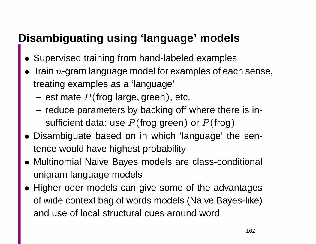
Disambiguating using ‘language’ models
• Supervised training from hand-labeled examples• Train n-gram language model for examples of each sense,
treating examples as a ‘language’– estimate P (frog|large, green), etc.– reduce parameters by backing off where there is in-
sufficient data: use P (frog|green) or P (frog)• Disambiguate based on in which ‘language’ the sen-
tence would have highest probability• Multinomial Naive Bayes models are class-conditional
unigram language models• Higher oder models can give some of the advantages
of wide context bag of words models (Naive Bayes-like)and use of local structural cues around word
162
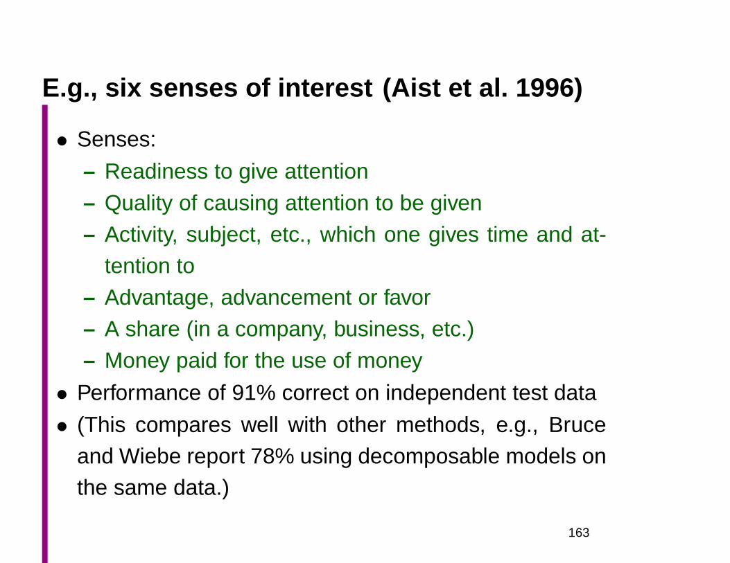
E.g., six senses of interest (Aist et al. 1996)
• Senses:
– Readiness to give attention– Quality of causing attention to be given– Activity, subject, etc., which one gives time and at-
tention to– Advantage, advancement or favor– A share (in a company, business, etc.)– Money paid for the use of money
• Performance of 91% correct on independent test data
• (This compares well with other methods, e.g., Bruceand Wiebe report 78% using decomposable models onthe same data.)
163
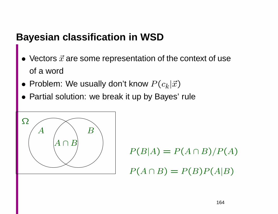
Bayesian classification in WSD
• Vectors ~x are some representation of the context of use
of a word
• Problem: We usually don’t know P (ck|~x)• Partial solution: we break it up by Bayes’ rule
A ∩B
ΩA B
P (B|A) = P (A ∩B)/P (A)
P (A ∩B) = P (B)P (A|B)
164
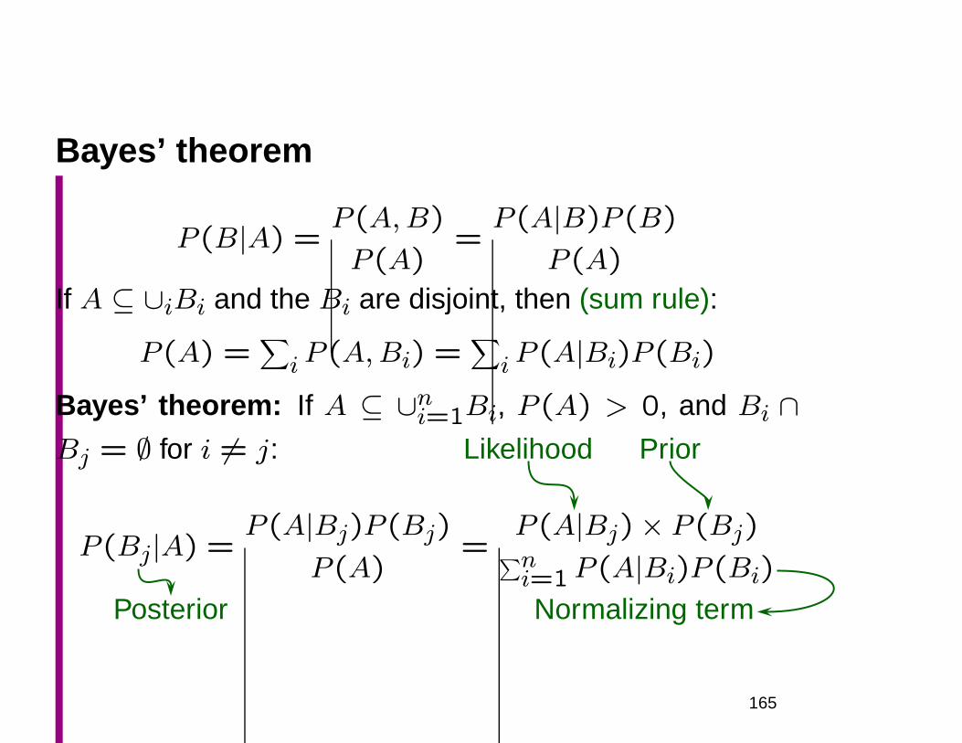
Bayes’ theorem
P (B|A) =P (A,B)
P (A)=P (A|B)P (B)
P (A)
If A ⊆ ∪iBi and the Bi are disjoint, then (sum rule):
P (A) =∑
iP (A,Bi) =∑
iP (A|Bi)P (Bi)
Bayes’ theorem: If A ⊆ ∪ni=1Bi, P (A) > 0, and Bi ∩Bj = ∅ for i 6= j: Likelihood Prior
P (Bj|A) =P (A|Bj)P (Bj)
P (A)=
P (A|Bj)× P (Bj)∑ni=1P (A|Bi)P (Bi)
Posterior Normalizing term
165
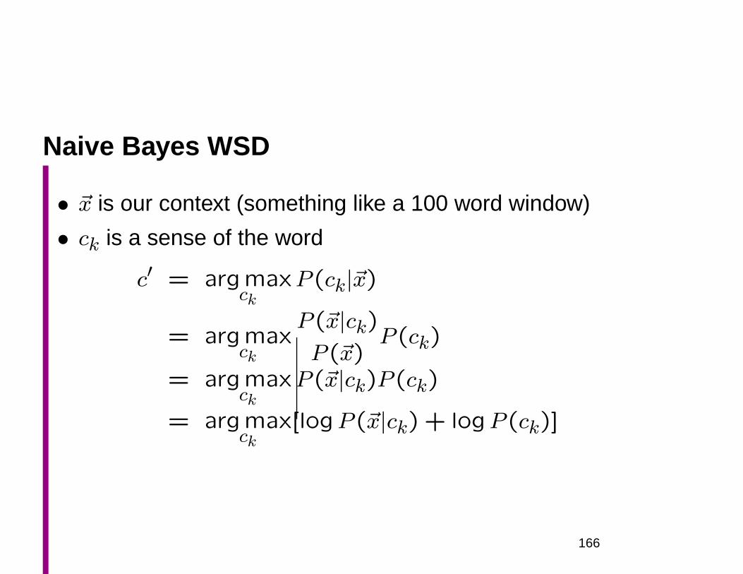
Naive Bayes WSD
• ~x is our context (something like a 100 word window)
• ck is a sense of the word
c′ = argmaxck
P (ck|~x)
= argmaxck
P (~x|ck)P (~x)
P (ck)
= argmaxck
P (~x|ck)P (ck)
= argmaxck
[logP (~x|ck) + logP (ck)]
166
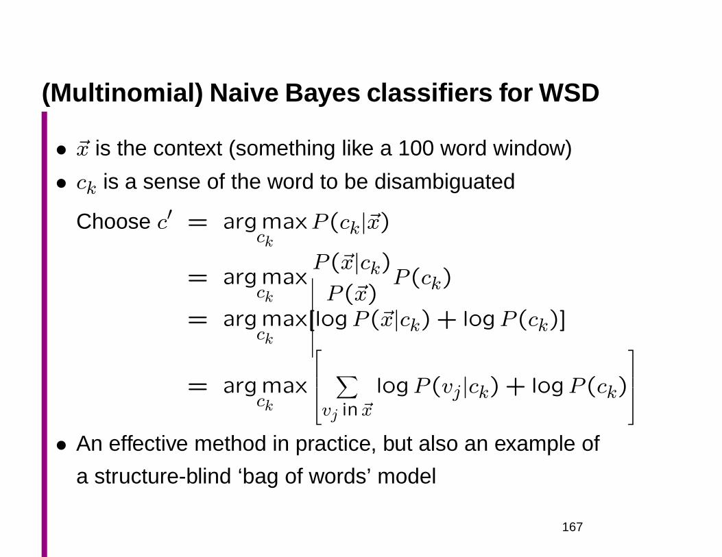
(Multinomial) Naive Bayes classifiers for WSD
• ~x is the context (something like a 100 word window)
• ck is a sense of the word to be disambiguated
Choose c′ = argmaxck
P (ck|~x)
= argmaxck
P (~x|ck)P (~x)
P (ck)
= argmaxck
[logP (~x|ck) + logP (ck)]
= argmaxck
∑
vj in ~x
logP (vj|ck) + logP (ck)
• An effective method in practice, but also an example of
a structure-blind ‘bag of words’ model
167
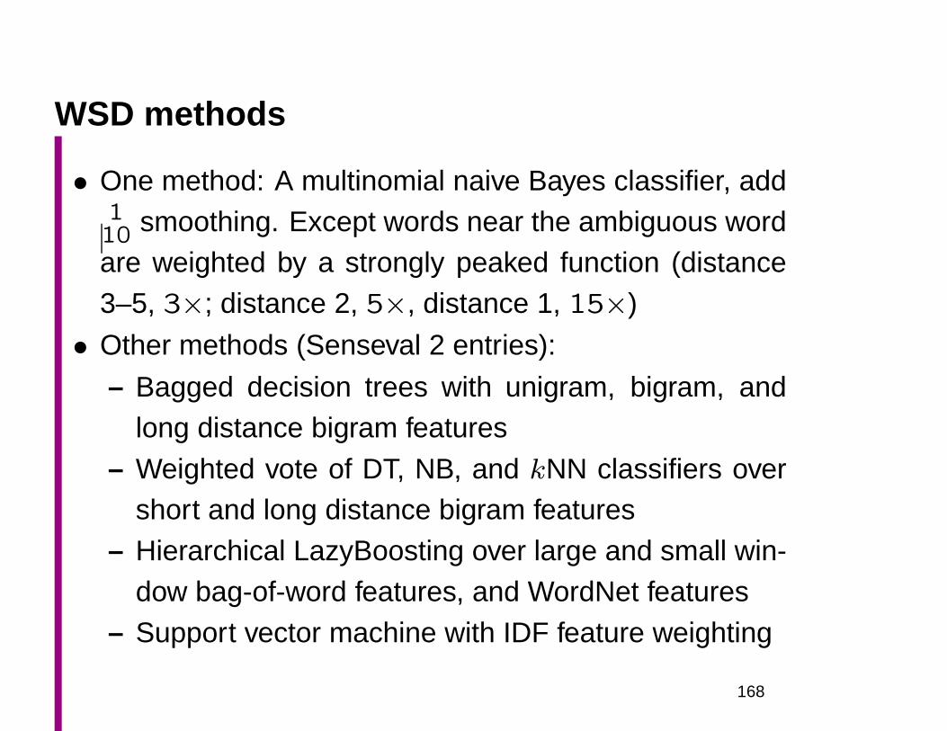
WSD methods
• One method: A multinomial naive Bayes classifier, add110 smoothing. Except words near the ambiguous wordare weighted by a strongly peaked function (distance3–5, 3×; distance 2, 5×, distance 1, 15×)
• Other methods (Senseval 2 entries):
– Bagged decision trees with unigram, bigram, andlong distance bigram features
– Weighted vote of DT, NB, and kNN classifiers overshort and long distance bigram features
– Hierarchical LazyBoosting over large and small win-dow bag-of-word features, and WordNet features
– Support vector machine with IDF feature weighting
168
Senseval 2 results
• The hacked Naive Bayes classifier has no particulartheoretical justification. One really cannot make senseof it in terms of the independence assumptions, etc.,usually invoked for a Naive Bayes model
• But it is linguistically roughly right: nearby context isoften very important for WSD: noun collocations (com-plete accident), verbs (derive satisfaction)
• In Senseval 2, it scores an average accuracy of 61.2%
• This model was just a component of a system we en-tered, but alone it would have come in 6th place out of27 systems (on English lexical sample data), beatingout all the systems on the previous slide
169
Word Sense Disambiguation
extra or variant slides
170
Word sense disambiguation
• The problem of assigning the correct sense to a use of
a word in context
• bank:
– the rising ground bordering a lake, river, or sea
– an establishment for the custody, loan exchange, or
issue of money
• Traders said central banks will be waiting in the wings.
• A straightforward classification problem
171
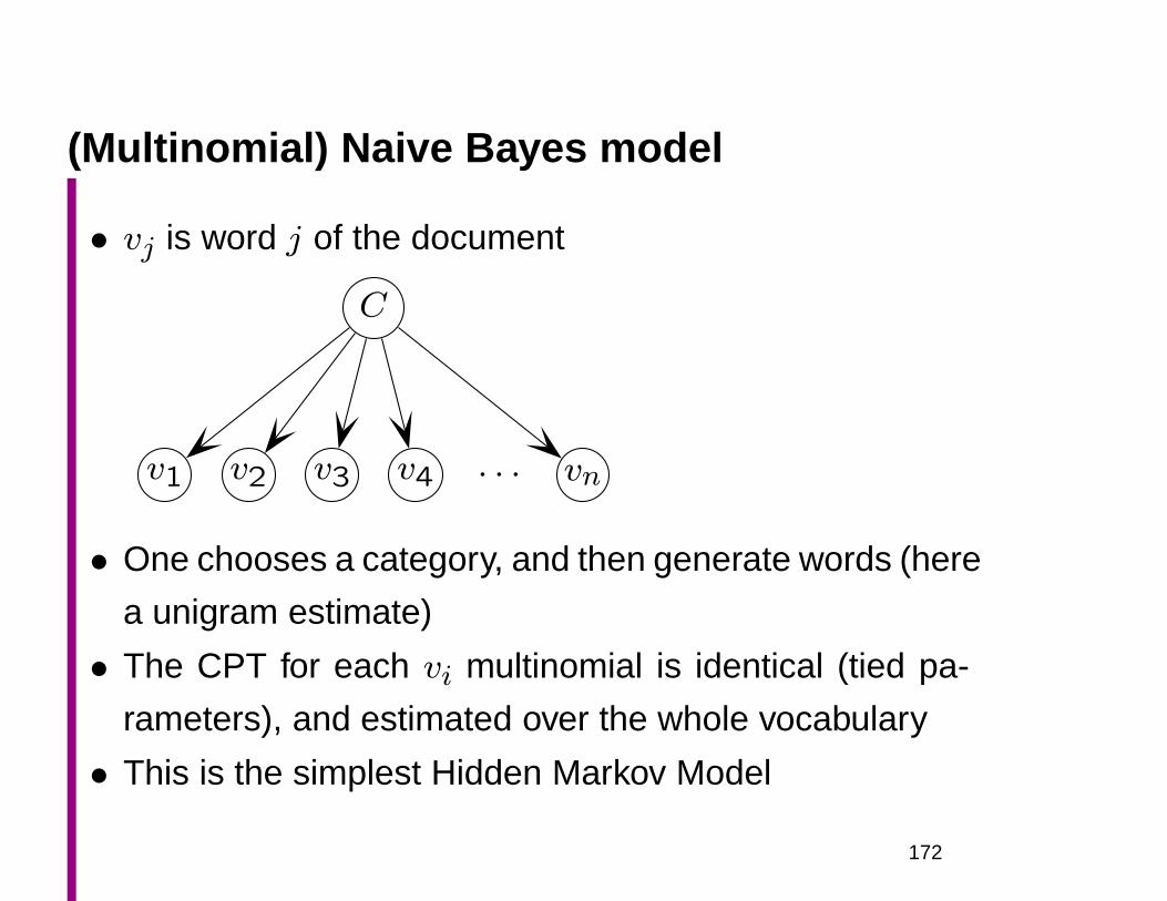
(Multinomial) Naive Bayes model
• vj is word j of the document
C
v1 v2 v3 v4 · · · vn
• One chooses a category, and then generate words (here
a unigram estimate)
• The CPT for each vi multinomial is identical (tied pa-
rameters), and estimated over the whole vocabulary
• This is the simplest Hidden Markov Model
172
Lexical Acquisition
FSNLP, chapter 8
Christopher Manning andHinrich Schütze
© 1999–2002
173
Lexical acquisition
• Language acquisition: acquiring the proper-
ties of words
• Practical: filling holes in dictionaries
– Language is productive
– Lots of stuff isn’t in dictionaries anyway
• Claim: most knowledge of language is encoded
in words.
174
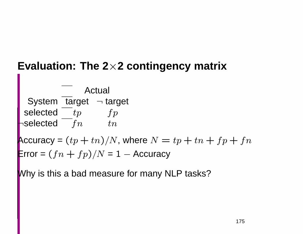
Evaluation: The 2 ×2 contingency matrix
ActualSystem target ¬ target
selected tp fp¬selected fn tn
Accuracy = (tp+ tn)/N , where N = tp+ tn+ fp+ fn
Error = (fn+ fp)/N = 1− Accuracy
Why is this a bad measure for many NLP tasks?
175
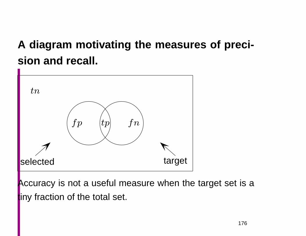
A diagram motivating the measures of preci-sion and recall.
tpfp fn
selected target
tn
Accuracy is not a useful measure when the target set is a
tiny fraction of the total set.
176
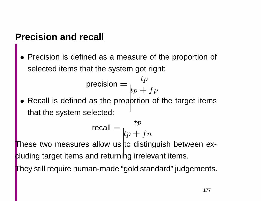
Precision and recall
• Precision is defined as a measure of the proportion of
selected items that the system got right:
precision =tp
tp+ fp
• Recall is defined as the proportion of the target items
that the system selected:
recall =tp
tp+ fn
These two measures allow us to distinguish between ex-
cluding target items and returning irrelevant items.
They still require human-made “gold standard” judgements.
177
A combined measure
Does one just average them? Bad, because the measures
aren’t independent.
What’s a sensible model?
Rijsbergen (1979:174) defines and justifies the usually used
alternative.
(see http://www.dcs.gla.ac.uk/Keith/Preface.html)
178
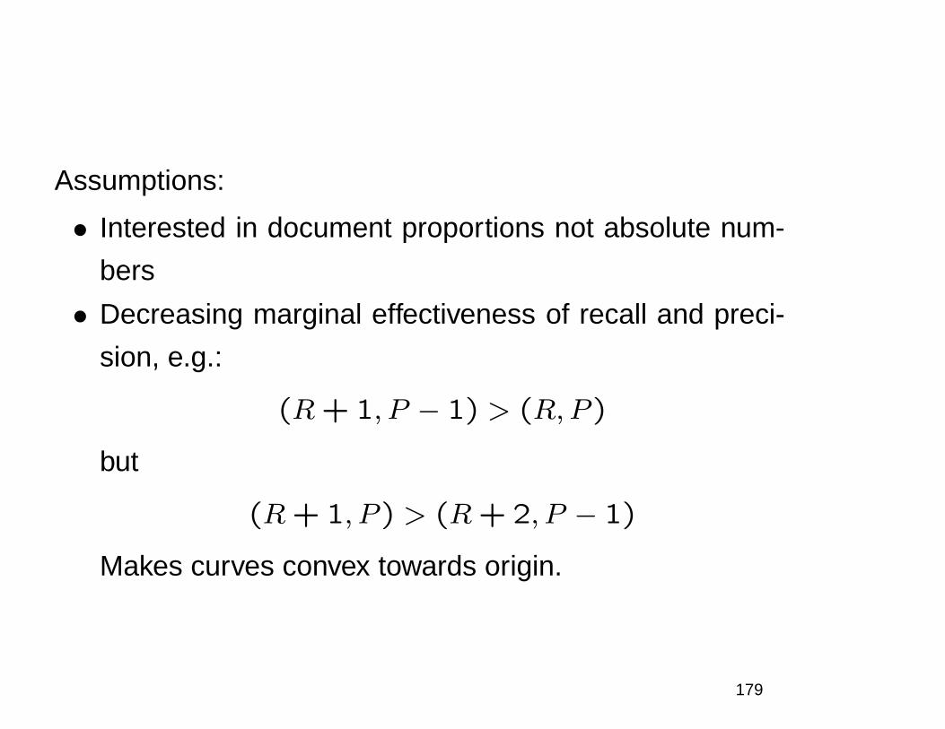
Assumptions:
• Interested in document proportions not absolute num-
bers
• Decreasing marginal effectiveness of recall and preci-
sion, e.g.:
(R+ 1, P − 1) > (R,P )
but
(R+ 1, P ) > (R+ 2, P − 1)
Makes curves convex towards origin.
179
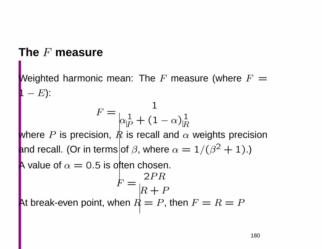
The F measure
Weighted harmonic mean: The F measure (where F =
1− E):
F =1
α1P + (1− α)1
R
where P is precision, R is recall and α weights precision
and recall. (Or in terms of β, where α = 1/(β2 + 1).)
A value of α = 0.5 is often chosen.
F =2PR
R+ P
At break-even point, when R = P , then F = R = P
180
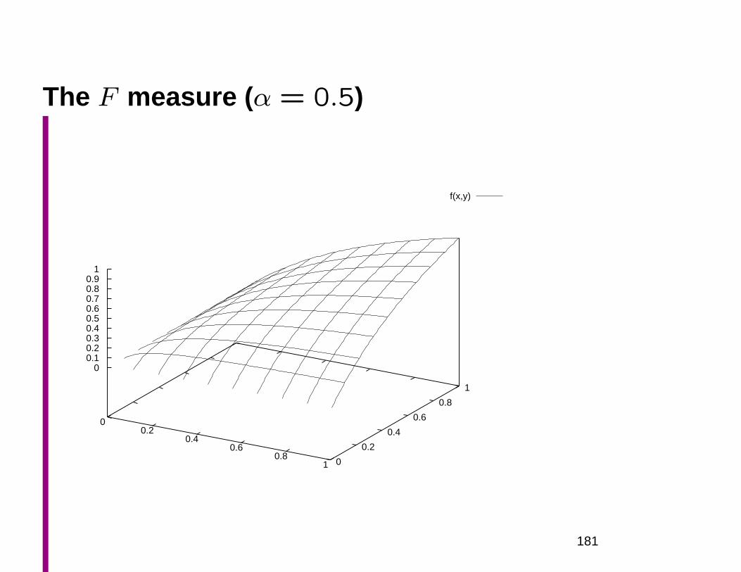
The F measure ( α = 0.5)
f(x,y)
00.2
0.40.6
0.81 0
0.2
0.4
0.6
0.8
1
00.10.20.30.40.50.60.70.80.9
1
181
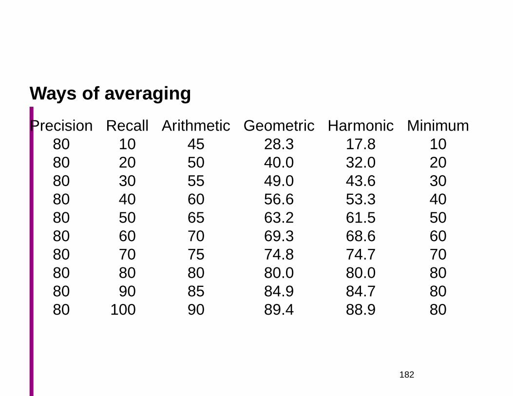
Ways of averaging
Precision Recall Arithmetic Geometric Harmonic Minimum80 10 45 28.3 17.8 1080 20 50 40.0 32.0 2080 30 55 49.0 43.6 3080 40 60 56.6 53.3 4080 50 65 63.2 61.5 5080 60 70 69.3 68.6 6080 70 75 74.8 74.7 7080 80 80 80.0 80.0 8080 90 85 84.9 84.7 8080 100 90 89.4 88.9 80
182
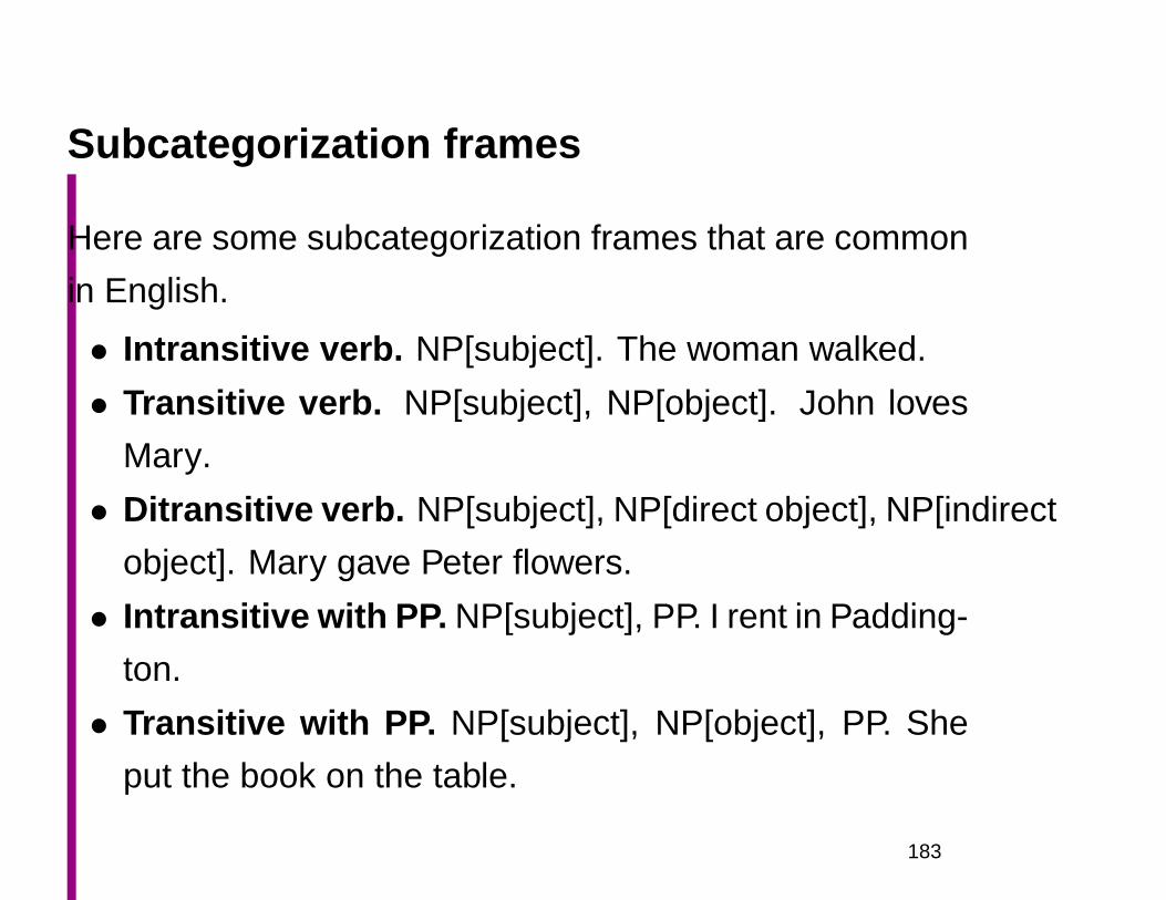
Subcategorization frames
Here are some subcategorization frames that are common
in English.
• Intransitive verb. NP[subject]. The woman walked.
• Transitive verb. NP[subject], NP[object]. John loves
Mary.
• Ditransitive verb. NP[subject], NP[direct object], NP[indirect
object]. Mary gave Peter flowers.
• Intransitive with PP. NP[subject], PP. I rent in Padding-
ton.
• Transitive with PP. NP[subject], NP[object], PP. She
put the book on the table.
183
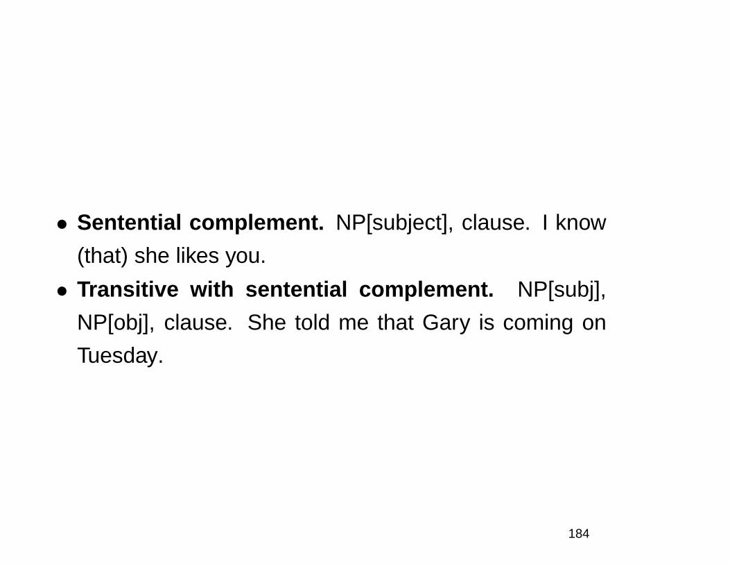
• Sentential complement. NP[subject], clause. I know
(that) she likes you.
• Transitive with sentential complement. NP[subj],
NP[obj], clause. She told me that Gary is coming on
Tuesday.
184
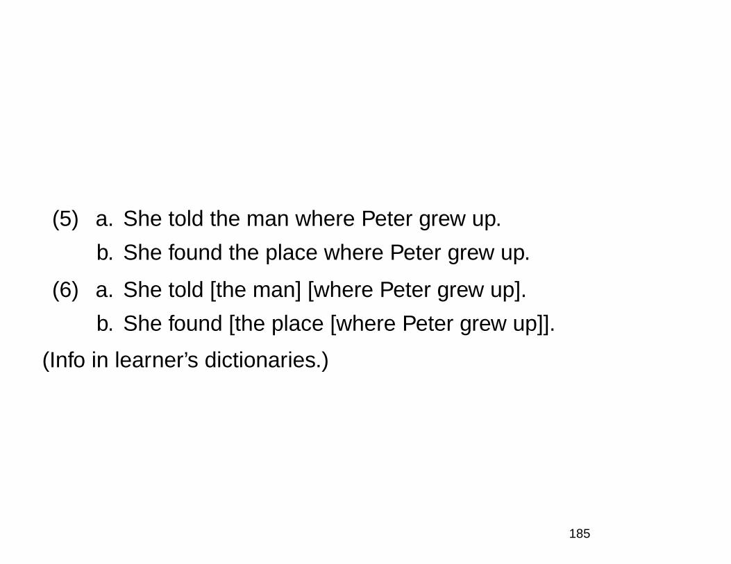
(5) a. She told the man where Peter grew up.
b. She found the place where Peter grew up.
(6) a. She told [the man] [where Peter grew up].
b. She found [the place [where Peter grew up]].
(Info in learner’s dictionaries.)
185
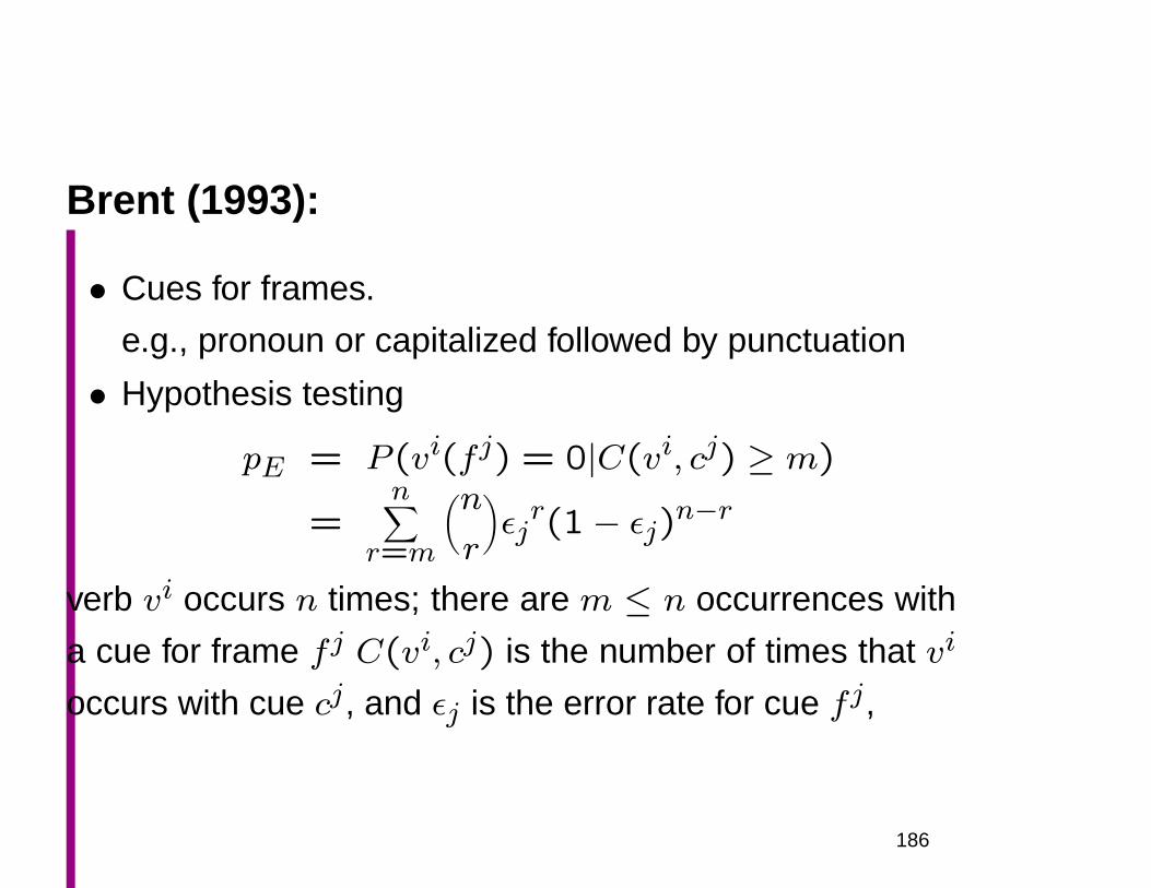
Brent (1993):
• Cues for frames.
e.g., pronoun or capitalized followed by punctuation
• Hypothesis testing
pE = P (vi(f j) = 0|C(vi, cj) ≥ m)
=n
∑
r=m
(n
r
)
ǫjr(1− ǫj)n−r
verb vi occurs n times; there are m ≤ n occurrences with
a cue for frame f j C(vi, cj) is the number of times that vi
occurs with cue cj, and ǫj is the error rate for cue f j,
186
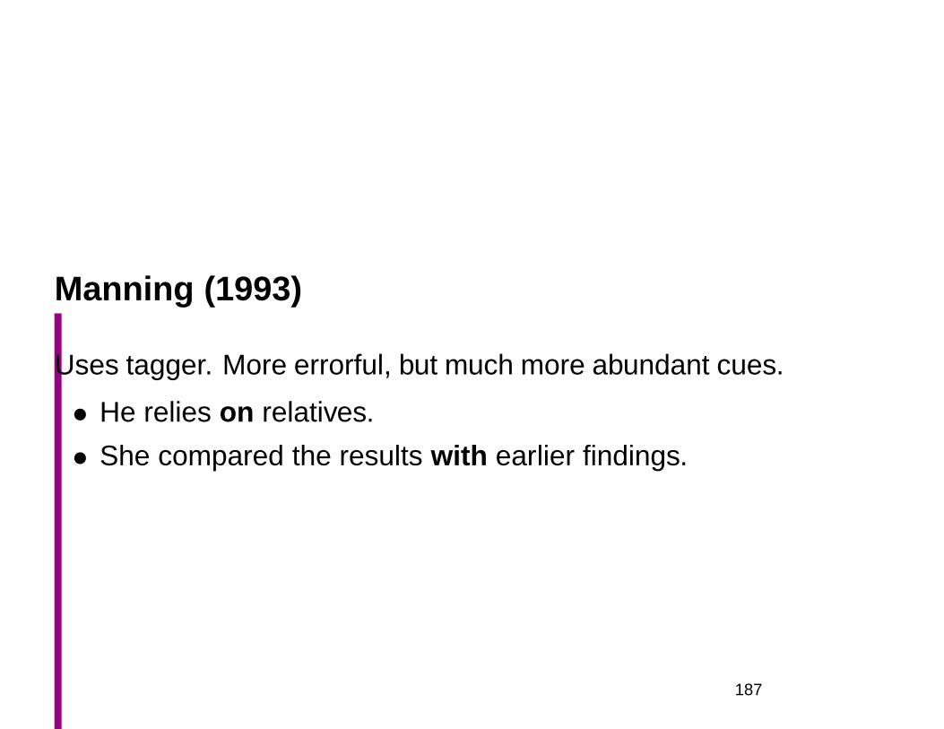
Manning (1993)
Uses tagger. More errorful, but much more abundant cues.
• He relies on relatives.
• She compared the results with earlier findings.
187

Learned subcategorization framesVerb Correct Incorrect OALD
bridge 1 1 1burden 2 2depict 2 3emanate 1 1leak 1 5occupy 1 3remark 1 1 4retire 2 1 5shed 1 2troop 0 3
188
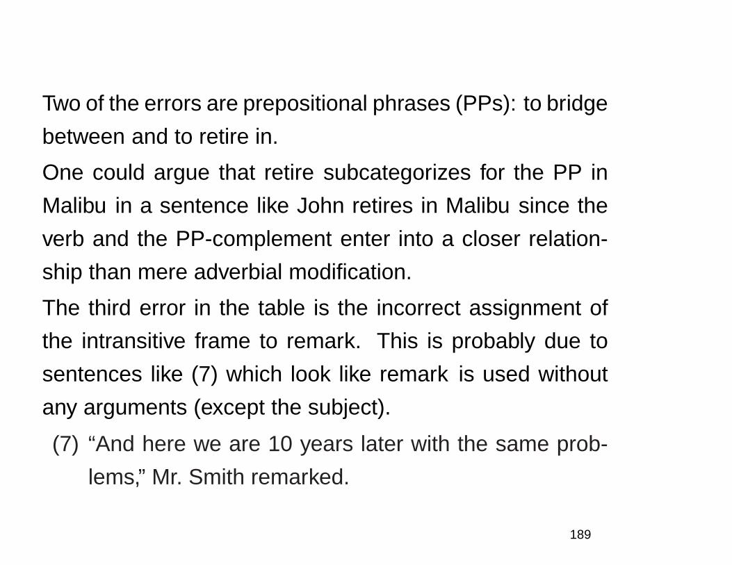
Two of the errors are prepositional phrases (PPs): to bridge
between and to retire in.
One could argue that retire subcategorizes for the PP in
Malibu in a sentence like John retires in Malibu since the
verb and the PP-complement enter into a closer relation-
ship than mere adverbial modification.
The third error in the table is the incorrect assignment of
the intransitive frame to remark. This is probably due to
sentences like (7) which look like remark is used without
any arguments (except the subject).
(7) “And here we are 10 years later with the same prob-
lems,” Mr. Smith remarked.
189
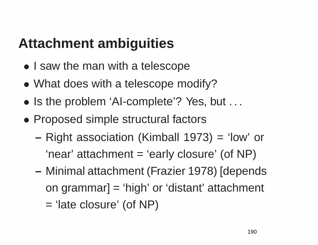
Attachment ambiguities
• I saw the man with a telescope
• What does with a telescope modify?
• Is the problem ‘AI-complete’? Yes, but . . .
• Proposed simple structural factors
– Right association (Kimball 1973) = ‘low’ or
‘near’ attachment = ‘early closure’ (of NP)
– Minimal attachment (Frazier 1978) [depends
on grammar] = ‘high’ or ‘distant’ attachment
= ‘late closure’ (of NP)
190
Attachment ambiguities (2)
• Such simple structural factors dominated in
early psycholinguistics, and are still widely in-
voked.
• In the V NP PP context, right attachment gets
right 55–67% of cases.
• But that means it gets wrong 33–45% of cases
191
Attachment ambiguities (3)
• The children ate the cake with a spoon.
• The children ate the cake with frosting.
• Moscow sent more than 100,000 soldiers into
Afghanistan . . .
• Sydney Water breached an agreement with
NSW Health . . .
Words are good predictors (even absent under-
standing).
192
Importance of lexical factors
Ford, Bresnan and Kaplan (1982) [as part of the
promotion of ‘lexicalist’ linguistic theories]
• Order of grammatical rule processing (by hu-
man) determines closure effects
• Ordering is jointly determined by strengths of
alternative lexical forms, strengths of alterna-
tive syntactic rewrite rules, and the sequence
of hypotheses in the parsing process
193
Importance of lexical factors (2)
Ford, Bresnan and Kaplan (1982):
• Joe included the package for Susan.
• Joe carried the package for Susan.
“It is quite evident, then, that the closure effects
in these sentences are induced in some way by
the choice of the lexical items.” (Psycholinguis-
tic studies show that this is true independent of
discourse context.)
194

Simple model
(Log) Likelihood Ratio [a common and good way
of comparing between two exclusive alternatives]
λ(v, n, p) = logP(p|v)P(p|n)
Problem: ignores preference for attaching “low”.
195
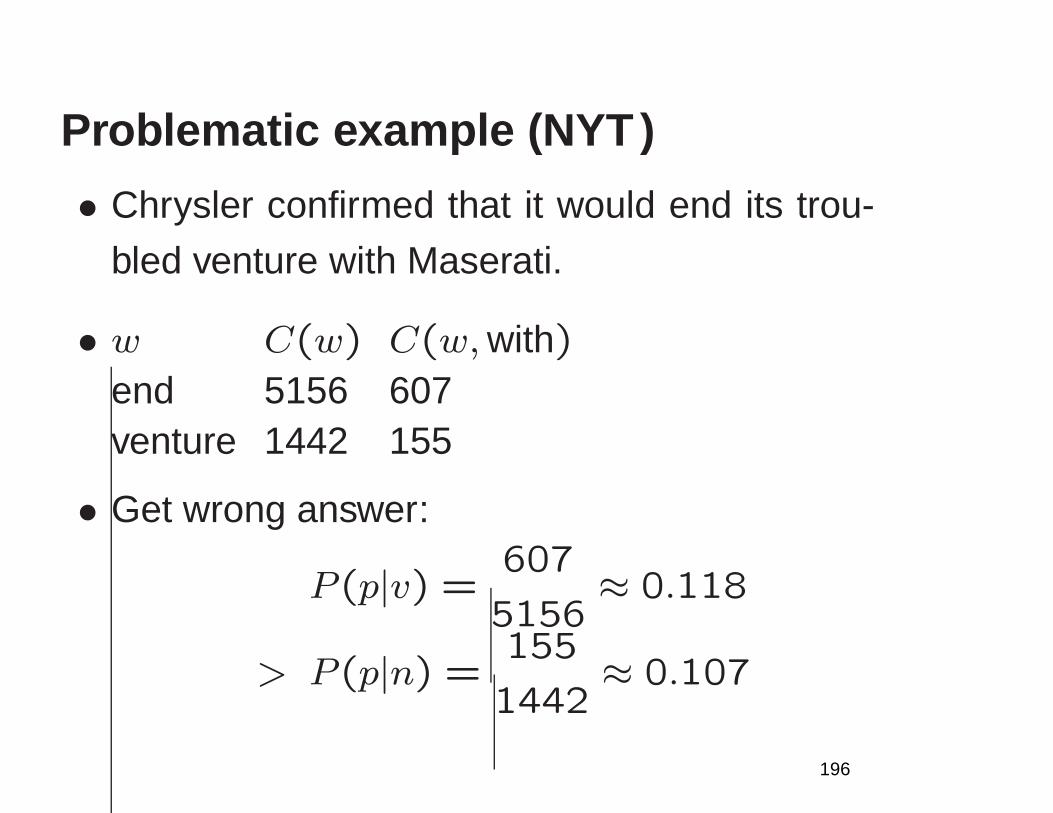
Problematic example ( NYT )
• Chrysler confirmed that it would end its trou-
bled venture with Maserati.
• w C(w) C(w,with)end 5156 607venture 1442 155
• Get wrong answer:
P(p|v) =607
5156≈ 0.118
> P (p|n) =155
1442≈ 0.107
196
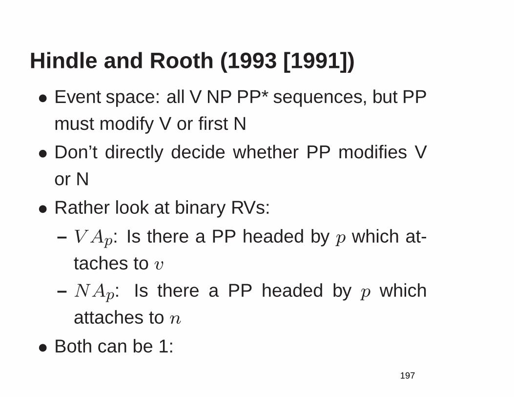
Hindle and Rooth (1993 [1991])
• Event space: all V NP PP* sequences, but PP
must modify V or first N
• Don’t directly decide whether PP modifies V
or N
• Rather look at binary RVs:
– V Ap: Is there a PP headed by p which at-
taches to v
– NAp: Is there a PP headed by p which
attaches to n
• Both can be 1:197

1
He put the book on World War II on the
table
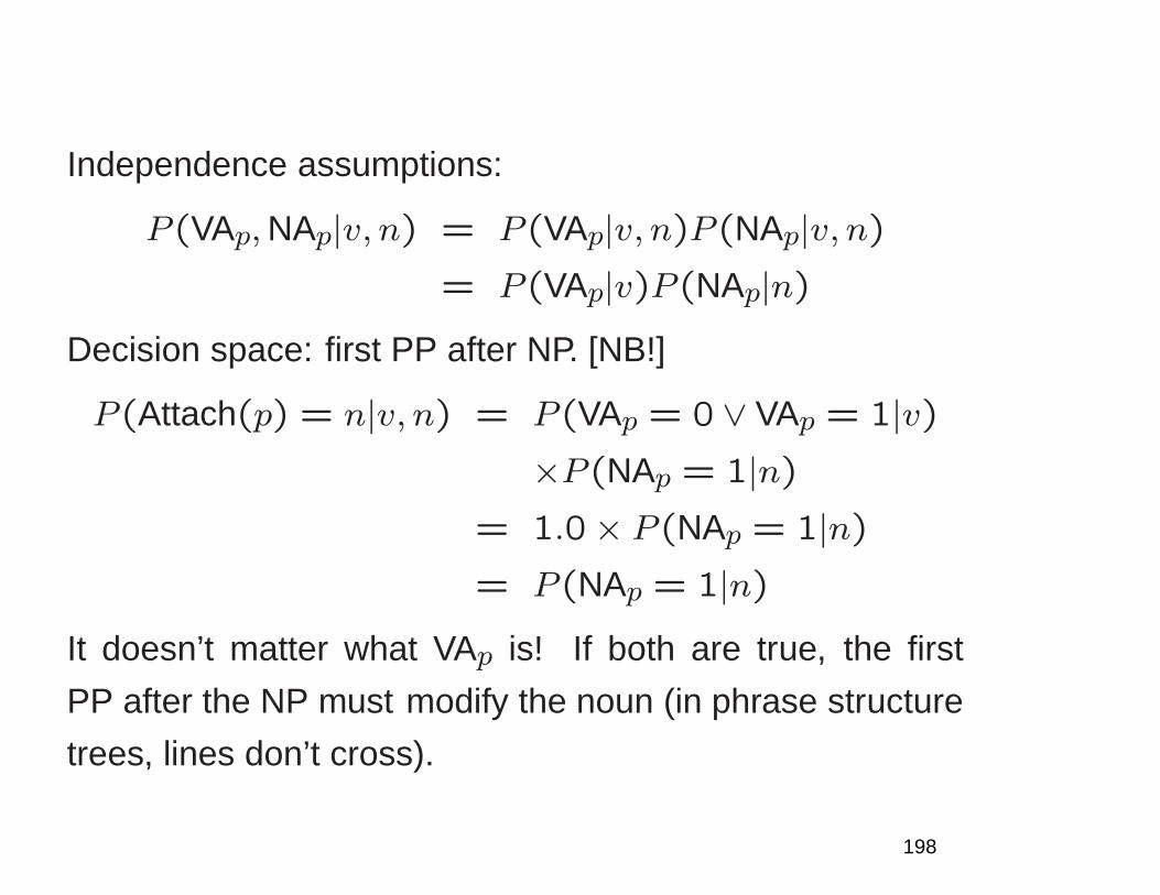
Independence assumptions:
P (VAp,NAp|v, n) = P (VAp|v, n)P (NAp|v, n)= P (VAp|v)P (NAp|n)
Decision space: first PP after NP. [NB!]
P (Attach(p) = n|v, n) = P (VAp = 0 ∨ VAp = 1|v)×P (NAp = 1|n)
= 1.0× P (NAp = 1|n)= P (NAp = 1|n)
It doesn’t matter what VAp is! If both are true, the first
PP after the NP must modify the noun (in phrase structure
trees, lines don’t cross).
198
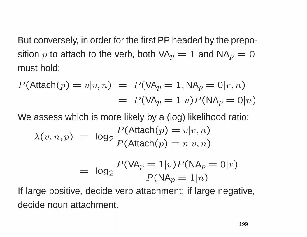
But conversely, in order for the first PP headed by the prepo-
sition p to attach to the verb, both VAp = 1 and NAp = 0
must hold:
P (Attach(p) = v|v, n) = P (VAp = 1,NAp = 0|v, n)= P (VAp = 1|v)P (NAp = 0|n)
We assess which is more likely by a (log) likelihood ratio:
λ(v, n, p) = log2P (Attach(p) = v|v, n)P (Attach(p) = n|v, n)
= log2P (VAp = 1|v)P (NAp = 0|v)
P (NAp = 1|n)If large positive, decide verb attachment; if large negative,
decide noun attachment.
199
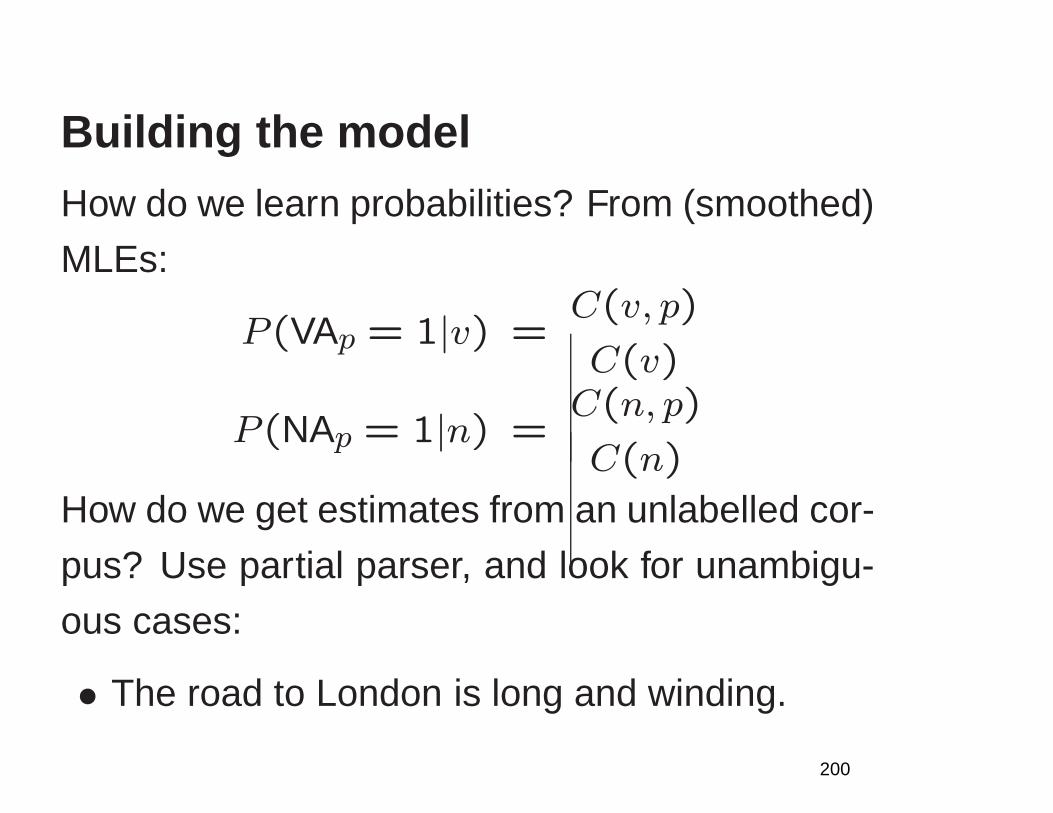
Building the model
How do we learn probabilities? From (smoothed)
MLEs:
P(VAp = 1|v) =C(v, p)
C(v)
P(NAp = 1|n) =C(n, p)
C(n)
How do we get estimates from an unlabelled cor-
pus? Use partial parser, and look for unambigu-
ous cases:
• The road to London is long and winding.
200

1
• She sent him into the nursery to gather up his
toys.
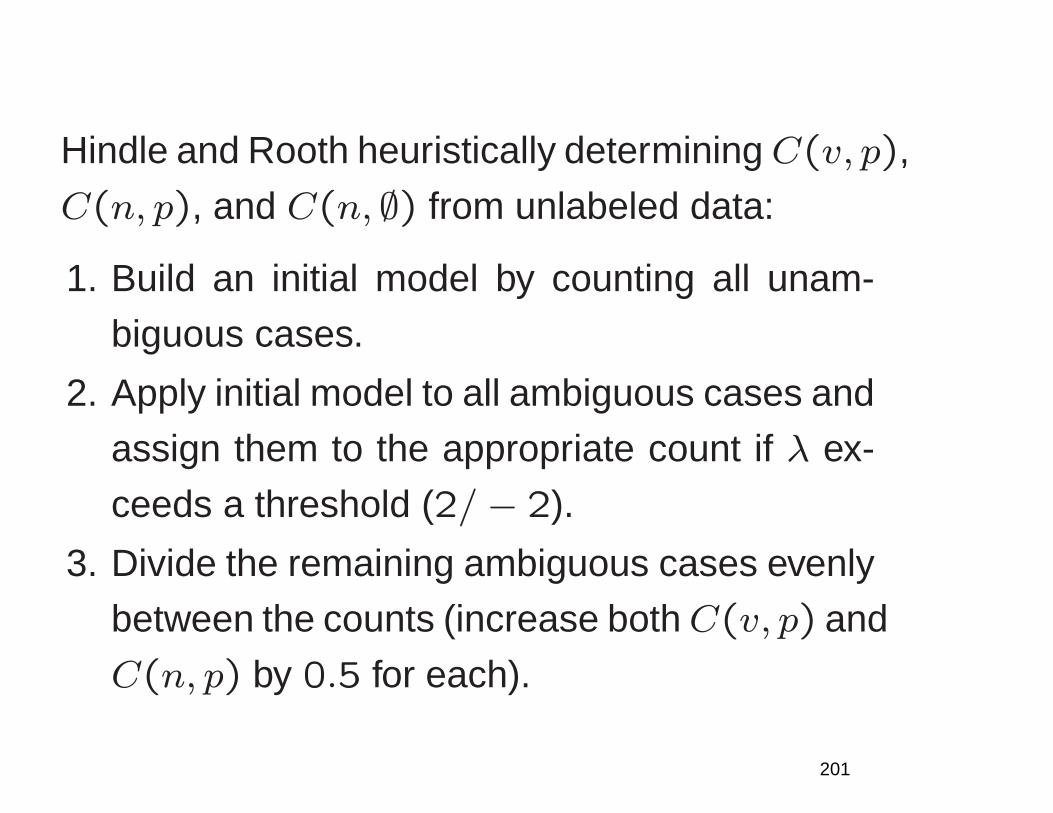
Hindle and Rooth heuristically determiningC(v, p),
C(n, p), and C(n, ∅) from unlabeled data:
1. Build an initial model by counting all unam-
biguous cases.
2. Apply initial model to all ambiguous cases and
assign them to the appropriate count if λ ex-
ceeds a threshold (2/− 2).
3. Divide the remaining ambiguous cases evenly
between the counts (increase bothC(v, p) and
C(n, p) by 0.5 for each).
201
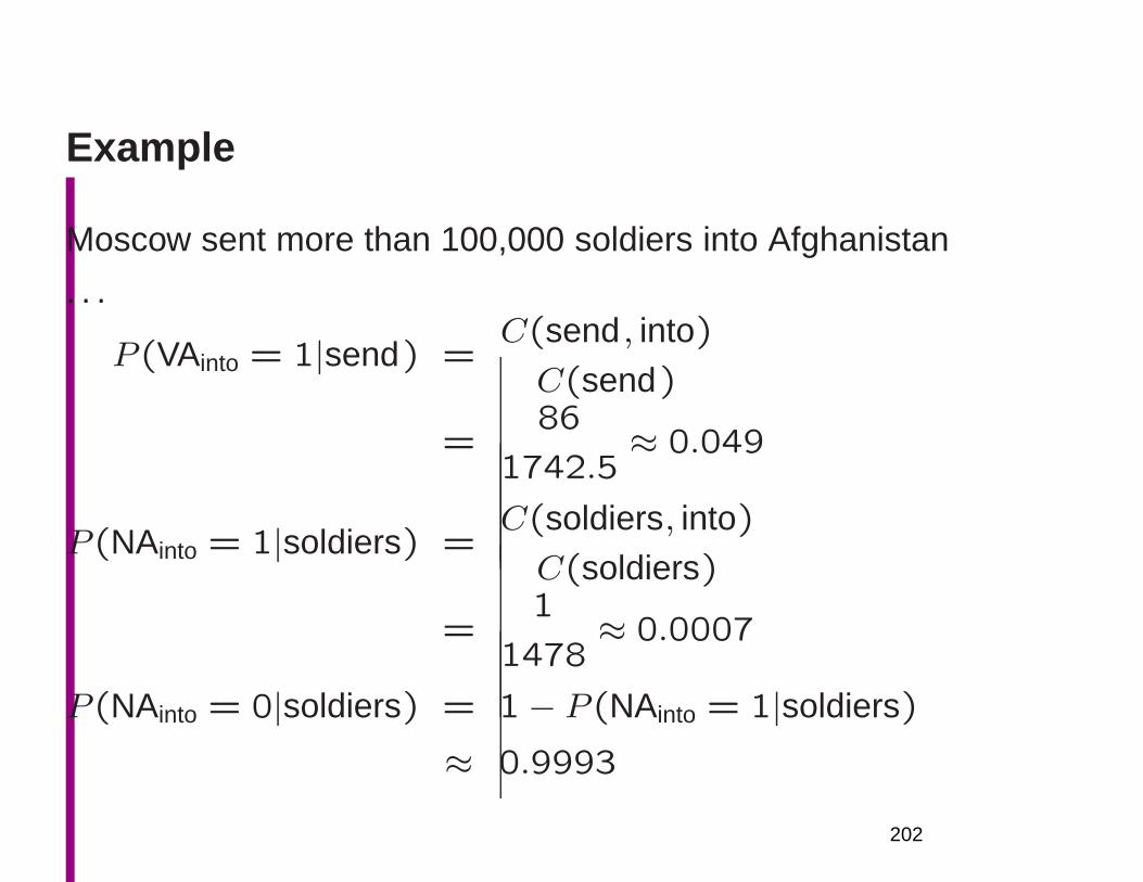
Example
Moscow sent more than 100,000 soldiers into Afghanistan
. . .
P (VAinto = 1|send) =C(send , into)
C(send)
=86
1742.5≈ 0.049
P (NAinto = 1|soldiers) =C(soldiers, into)
C(soldiers)
=1
1478≈ 0.0007
P (NAinto = 0|soldiers) = 1− P (NAinto = 1|soldiers)
≈ 0.9993
202
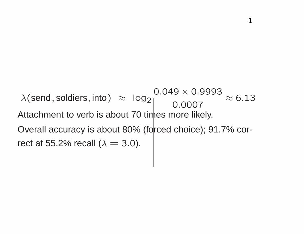
1
λ(send , soldiers, into) ≈ log20.049× 0.9993
0.0007≈ 6.13
Attachment to verb is about 70 times more likely.
Overall accuracy is about 80% (forced choice); 91.7% cor-
rect at 55.2% recall (λ = 3.0).
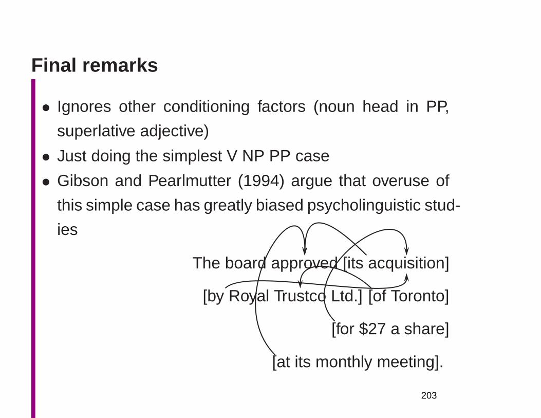
Final remarks
• Ignores other conditioning factors (noun head in PP,
superlative adjective)
• Just doing the simplest V NP PP case
• Gibson and Pearlmutter (1994) argue that overuse of
this simple case has greatly biased psycholinguistic stud-
ies
The board approved [its acquisition]
[by Royal Trustco Ltd.] [of Toronto]
[for $27 a share]
[at its monthly meeting].
203
Final remarks (2)
• There are other attachment cases: coordina-
tion, adverbial and participial phrases, noun
compounds. Data sparseness is a bigger prob-
lem with many of these (more open class heads
needed).
• In general, indeterminacy is quite common:
We have not signed a settlement agree-
ment with them.
Either reading seems equally plausible.
204
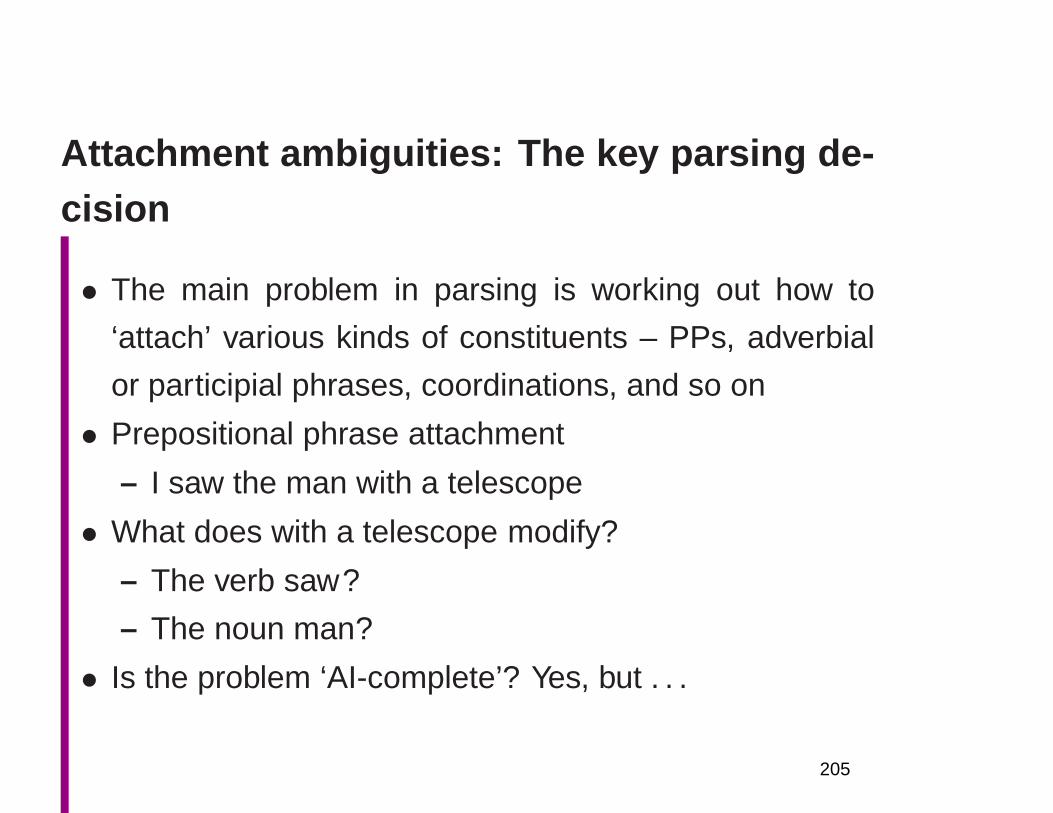
Attachment ambiguities: The key parsing de-cision
• The main problem in parsing is working out how to
‘attach’ various kinds of constituents – PPs, adverbial
or participial phrases, coordinations, and so on
• Prepositional phrase attachment
– I saw the man with a telescope
• What does with a telescope modify?
– The verb saw?
– The noun man?
• Is the problem ‘AI-complete’? Yes, but . . .
205

S
NP
PRP
I
VP
V
VBD
saw
NP
DT
the
NN
man
PP
IN
with
NP
DT
a
NN
telescope
S
NP
PRP
I
VP
V
VBD
saw
v
NP
NP
DT
the
NN
man
n1
PP
IN
with
p
NP
DT
a
NN
telescope
n2
206

Attachment ambiguities (2)
• Proposed simple structural factors
– Right association (Kimball 1973) = ‘low’ or ‘near’ at-
tachment = ‘late closure’ (of NP) [NP→ NP PP]
– Minimal attachment (Frazier 1978) [depends on gram-
mar] = ‘high’ or ‘distant’ attachment = ‘early closure’
(of NP) [VP→ V NP PP]
• Such simple structural factors dominated in early psy-
cholinguistics, and are still widely invoked.
• In the V NP PP context, right attachment gets it right in
55–67% of cases.
• But that means it gets it wrong in 33–45% of cases
207
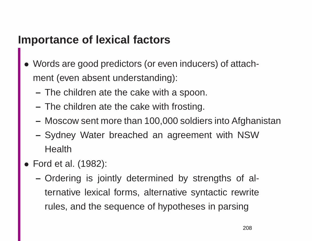
Importance of lexical factors
• Words are good predictors (or even inducers) of attach-
ment (even absent understanding):
– The children ate the cake with a spoon.
– The children ate the cake with frosting.
– Moscow sent more than 100,000 soldiers into Afghanistan
– Sydney Water breached an agreement with NSW
Health
• Ford et al. (1982):
– Ordering is jointly determined by strengths of al-
ternative lexical forms, alternative syntactic rewrite
rules, and the sequence of hypotheses in parsing
208

Simple model
(Log) Likelihood Ratio [a common and good way
of comparing between two exclusive alternatives]
λ(v, n, p) = logP(p|v)P(p|n)
Problem: ignores preference for attaching “low”
209

Problematic example ( NYT )
• Chrysler confirmed that it would end its trou-
bled venture with Maserati.
• w C(w) C(w,with)end 5156 607venture 1442 155
• Get wrong answer:
P(p|v) =607
5156≈ 0.118
> P (p|n) =155
1442≈ 0.107
210
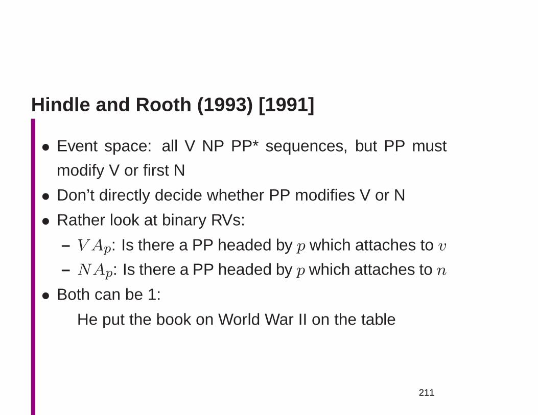
Hindle and Rooth (1993) [1991]
• Event space: all V NP PP* sequences, but PP must
modify V or first N
• Don’t directly decide whether PP modifies V or N
• Rather look at binary RVs:
– V Ap: Is there a PP headed by p which attaches to v
– NAp: Is there a PP headed by p which attaches to n
• Both can be 1:
He put the book on World War II on the table
211
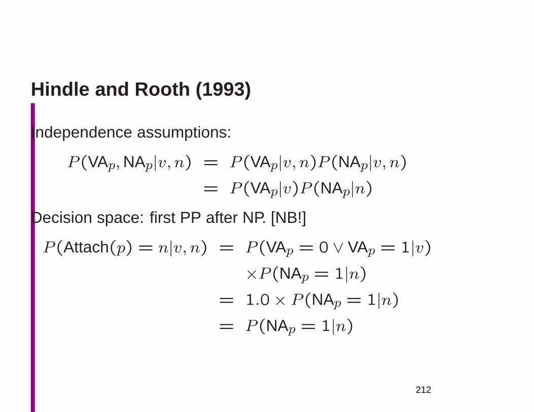
Hindle and Rooth (1993)
Independence assumptions:
P (VAp,NAp|v, n) = P (VAp|v, n)P (NAp|v, n)= P (VAp|v)P (NAp|n)
Decision space: first PP after NP. [NB!]
P (Attach(p) = n|v, n) = P (VAp = 0 ∨ VAp = 1|v)×P (NAp = 1|n)
= 1.0× P (NAp = 1|n)= P (NAp = 1|n)
212
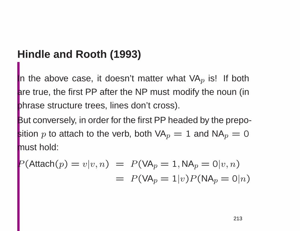
Hindle and Rooth (1993)
In the above case, it doesn’t matter what VAp is! If both
are true, the first PP after the NP must modify the noun (in
phrase structure trees, lines don’t cross).
But conversely, in order for the first PP headed by the prepo-
sition p to attach to the verb, both VAp = 1 and NAp = 0
must hold:
P (Attach(p) = v|v, n) = P (VAp = 1,NAp = 0|v, n)= P (VAp = 1|v)P (NAp = 0|n)
213
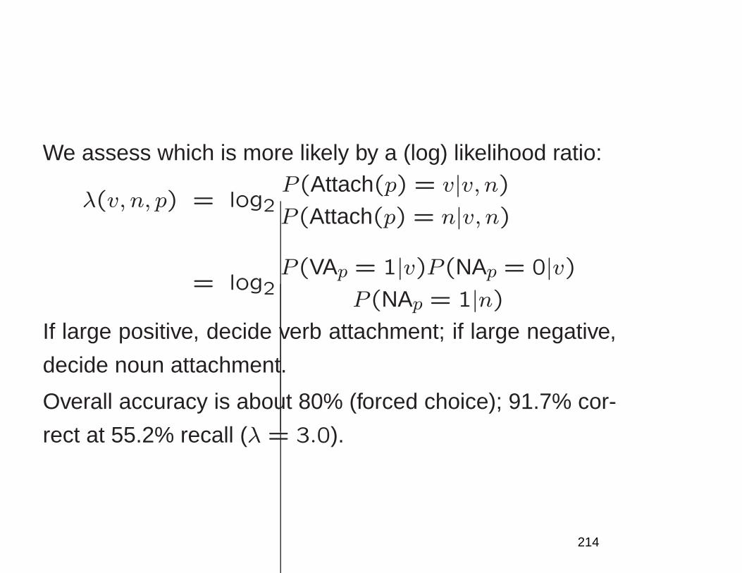
We assess which is more likely by a (log) likelihood ratio:
λ(v, n, p) = log2P (Attach(p) = v|v, n)P (Attach(p) = n|v, n)
= log2P (VAp = 1|v)P (NAp = 0|v)
P (NAp = 1|n)If large positive, decide verb attachment; if large negative,
decide noun attachment.
Overall accuracy is about 80% (forced choice); 91.7% cor-
rect at 55.2% recall (λ = 3.0).
214
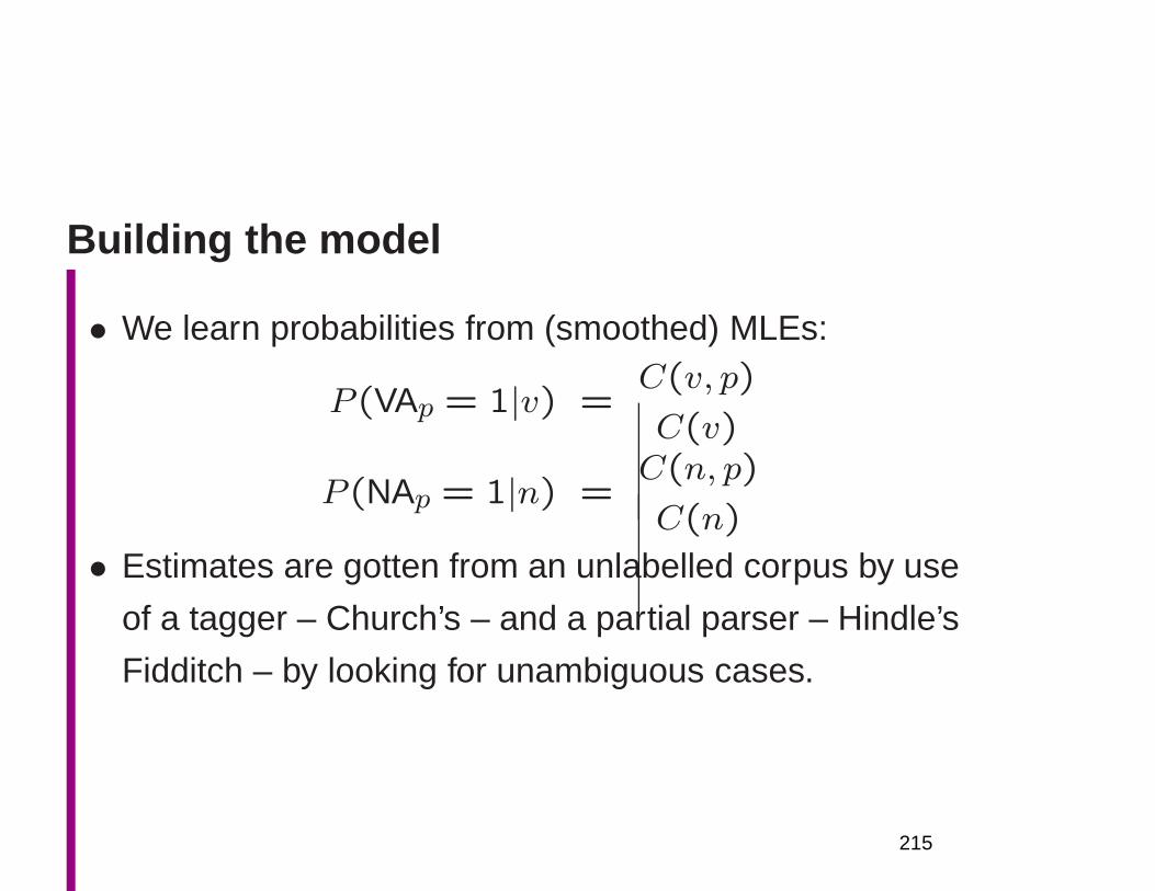
Building the model
• We learn probabilities from (smoothed) MLEs:
P (VAp = 1|v) =C(v, p)
C(v)
P (NAp = 1|n) =C(n, p)
C(n)
• Estimates are gotten from an unlabelled corpus by use
of a tagger – Church’s – and a partial parser – Hindle’s
Fidditch – by looking for unambiguous cases.
215
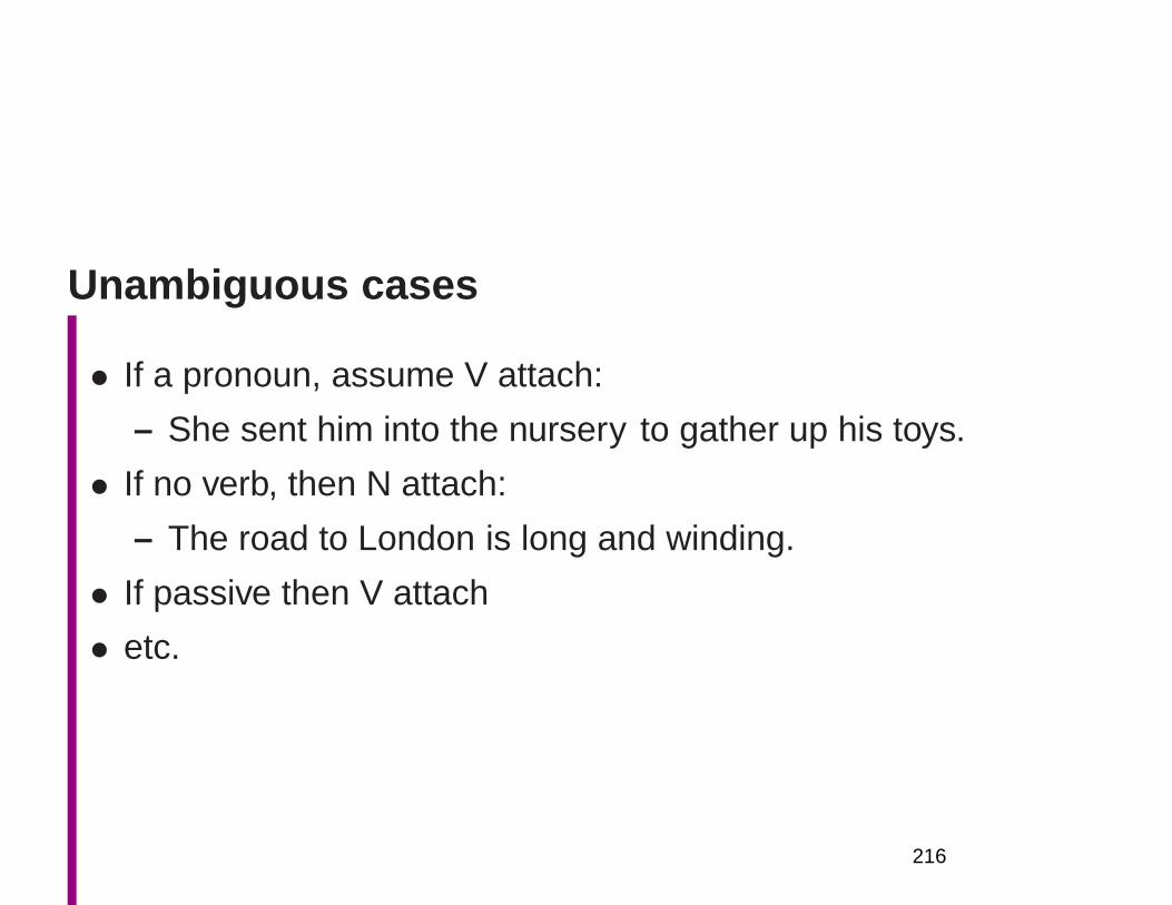
Unambiguous cases
• If a pronoun, assume V attach:
– She sent him into the nursery to gather up his toys.
• If no verb, then N attach:
– The road to London is long and winding.
• If passive then V attach
• etc.
216
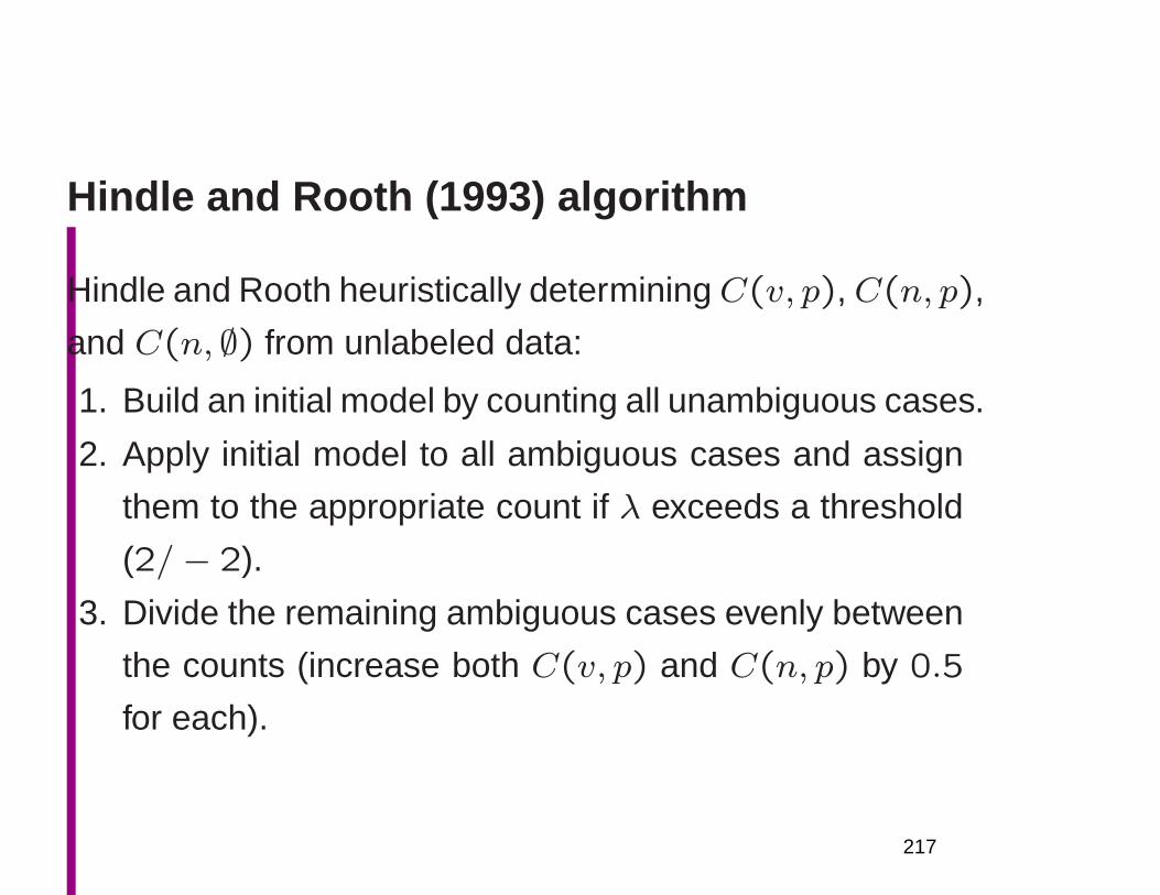
Hindle and Rooth (1993) algorithm
Hindle and Rooth heuristically determiningC(v, p),C(n, p),
and C(n, ∅) from unlabeled data:
1. Build an initial model by counting all unambiguous cases.
2. Apply initial model to all ambiguous cases and assign
them to the appropriate count if λ exceeds a threshold
(2/− 2).
3. Divide the remaining ambiguous cases evenly between
the counts (increase both C(v, p) and C(n, p) by 0.5
for each).
217
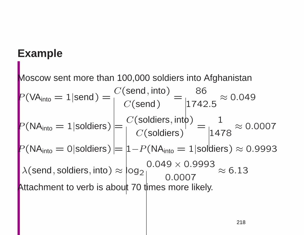
Example
Moscow sent more than 100,000 soldiers into Afghanistan
P (VAinto = 1|send) =C(send , into)
C(send)=
86
1742.5≈ 0.049
P (NAinto = 1|soldiers) =C(soldiers, into)
C(soldiers)=
1
1478≈ 0.0007
P (NAinto = 0|soldiers) = 1−P (NAinto = 1|soldiers) ≈ 0.9993
λ(send , soldiers, into) ≈ log20.049× 0.9993
0.0007≈ 6.13
Attachment to verb is about 70 times more likely.
218

Collins and Brooks (1995)
• Use fully parsed treebank data
• Includes n2 in model: quadruples 〈v, n1, p, n2〉• Uses a back-off model to address data sparseness is-
sues.
• About 95% of test quadruples not seen in training data
• Start with full quadruples, backoff to triples and pairs
restricted so as to always contain p
• Accuracy: 86.5%
219
More complex situations
• Hindle and Rooth (1993) – and Collins and Brooks (1995)
– are just doing the simplest V NP PP case
• Gibson and Pearlmutter (1994) argue that overuse of
this simple case has greatly biased psycholinguistic stud-
ies
• V NP PP PP has 5 possible attachments; V NP PP PP PP
has 14
• The problem is much harder, and a dumb algorithm will
perform poorly
220
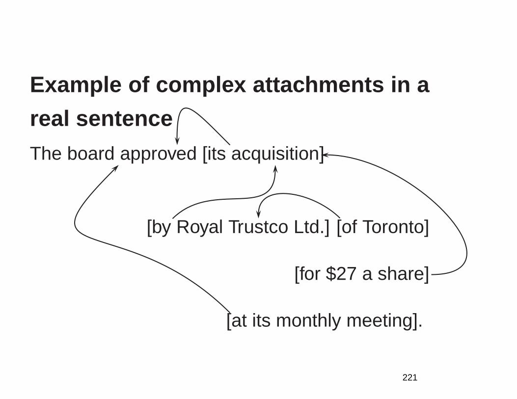
Example of complex attachments in a
real sentence
The board approved [its acquisition]
[by Royal Trustco Ltd.] [of Toronto]
[for $27 a share]
[at its monthly meeting].
221
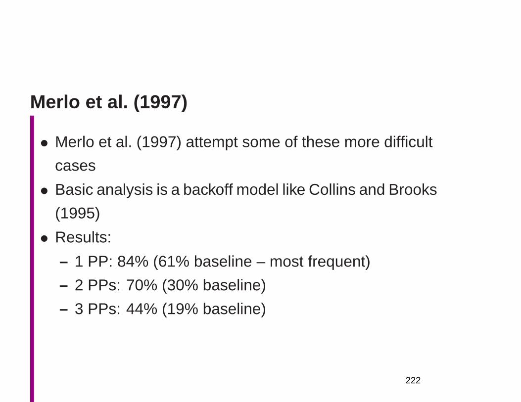
Merlo et al. (1997)
• Merlo et al. (1997) attempt some of these more difficult
cases
• Basic analysis is a backoff model like Collins and Brooks
(1995)
• Results:
– 1 PP: 84% (61% baseline – most frequent)
– 2 PPs: 70% (30% baseline)
– 3 PPs: 44% (19% baseline)
222
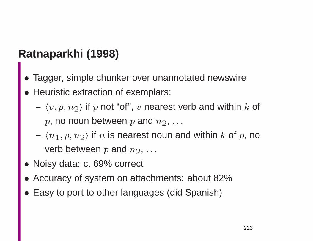
Ratnaparkhi (1998)
• Tagger, simple chunker over unannotated newswire
• Heuristic extraction of exemplars:
– 〈v, p, n2〉 if p not “of”, v nearest verb and within k of
p, no noun between p and n2, . . .
– 〈n1, p, n2〉 if n is nearest noun and within k of p, no
verb between p and n2, . . .
• Noisy data: c. 69% correct
• Accuracy of system on attachments: about 82%
• Easy to port to other languages (did Spanish)
223
Final remarks
• Many other similar sorts of attachment decisions: coor-
dination, adverbial and participial phrases, noun com-
pounds
– I drink [coffee with [cream and sugar]]
– I drink [[coffee with cream] and sugar]
• Data sparseness is a bigger problem with many of these
(more open class heads needed).
• In general, indeterminacy is quite common:
– We have not signed a settlement agreement with
them.
224
Lexical acquisition
• Simple statistical models give same estimate
to all unseen events
• Unrealistic – could hope to refine that based
on semantic classes of words
• E.g, although never seen, eating pineapple
should be more likely than eating holograms
because pineapple is similar to apples, and
we have seen eating apples
• It’s the same data. Why are classes useful?
225
An application: selectional preferences
• Verbs take arguments of certain types (usually! – re-member metaphor)• Bill drove a . . .• Mustang, car, truck, jeep, . . .• Resnik (1993) uses KL divergence for verb objects dis-
tributions• Selectional preference strength: how strongly does a
verb constrain direct objects• see vs. unknotted• Model via using head words only – a usually correct
assumption• Use a class-based model of nouns – for generalization.
Resnik uses WordNet.
226
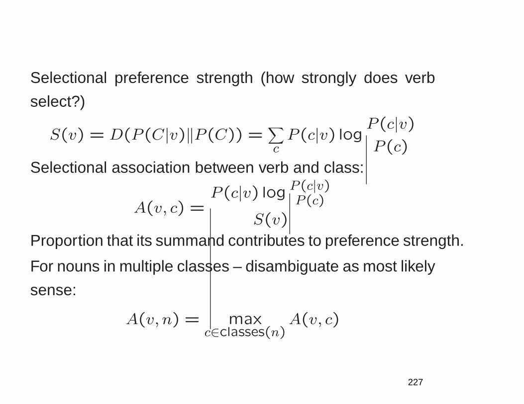
Selectional preference strength (how strongly does verb
select?)
S(v) = D(P (C|v)‖P (C)) =∑
cP (c|v) log
P (c|v)P (c)
Selectional association between verb and class:
A(v, c) =P (c|v) log
P(c|v)P(c)
S(v)
Proportion that its summand contributes to preference strength.
For nouns in multiple classes – disambiguate as most likely
sense:
A(v, n) = maxc∈classes(n)
A(v, c)
227
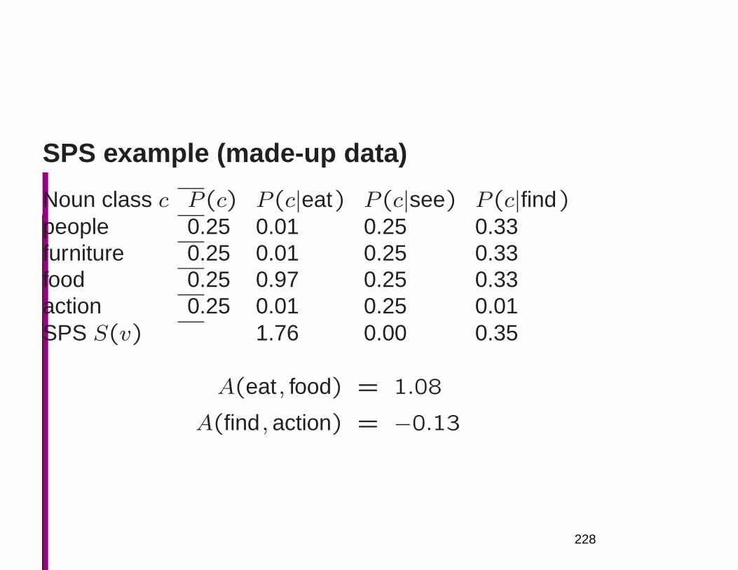
SPS example (made-up data)
Noun class c P (c) P (c|eat) P (c|see) P (c|find)
people 0.25 0.01 0.25 0.33furniture 0.25 0.01 0.25 0.33food 0.25 0.97 0.25 0.33action 0.25 0.01 0.25 0.01SPS S(v) 1.76 0.00 0.35
A(eat , food) = 1.08
A(find , action) = −0.13
228
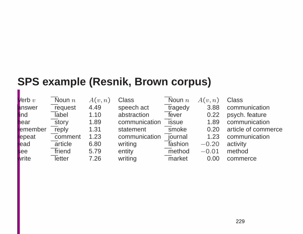
SPS example (Resnik, Brown corpus)
Verb v Noun n A(v, n) Class Noun n A(v, n) Classanswer request 4.49 speech act tragedy 3.88 communicationfind label 1.10 abstraction fever 0.22 psych. featurehear story 1.89 communication issue 1.89 communicationremember reply 1.31 statement smoke 0.20 article of commercerepeat comment 1.23 communication journal 1.23 communicationread article 6.80 writing fashion −0.20 activitysee friend 5.79 entity method −0.01 methodwrite letter 7.26 writing market 0.00 commerce
229

But how might we measure word sim-
ilarity for word classes?
Vector spaces
A document-by-word matrix A.cosmonaut astronaut moon car truck
d1 1 0 1 1 0d2 0 1 1 0 0d3 1 0 0 0 0d4 0 0 0 1 1d5 0 0 0 1 0d6 0 0 0 0 1
230
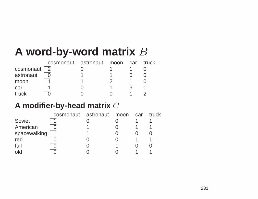
A word-by-word matrix Bcosmonaut astronaut moon car truck
cosmonaut 2 0 1 1 0astronaut 0 1 1 0 0moon 1 1 2 1 0car 1 0 1 3 1truck 0 0 0 1 2
A modifier-by-head matrix Ccosmonaut astronaut moon car truck
Soviet 1 0 0 1 1American 0 1 0 1 1spacewalking 1 1 0 0 0red 0 0 0 1 1full 0 0 1 0 0old 0 0 0 1 1
231
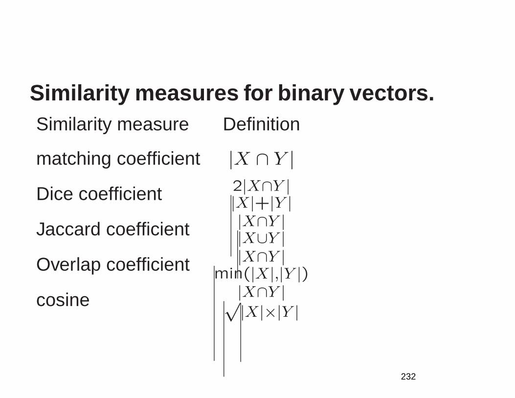
Similarity measures for binary vectors.Similarity measure Definition
matching coefficient |X ∩ Y |Dice coefficient 2|X∩Y |
|X|+|Y |Jaccard coefficient |X∩Y |
|X∪Y |Overlap coefficient |X∩Y |
min(|X|,|Y |)cosine |X∩Y |√
|X|×|Y |
232
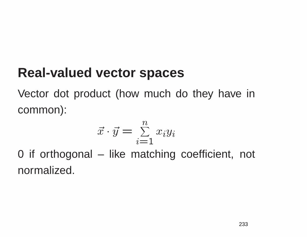
Real-valued vector spaces
Vector dot product (how much do they have in
common):
~x · ~y =n∑
i=1xiyi
0 if orthogonal – like matching coefficient, not
normalized.
233
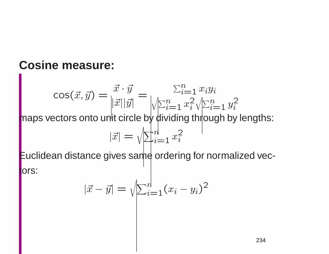
Cosine measure:
cos(~x, ~y) =~x · ~y|~x||~y| =
∑ni=1 xiyi
√
∑ni=1 x
2i
√
∑ni=1 y
2i
maps vectors onto unit circle by dividing through by lengths:
|~x| =√
∑ni=1 x
2i
Euclidean distance gives same ordering for normalized vec-
tors:
|~x− ~y| =√
∑ni=1(xi − yi)
2
234
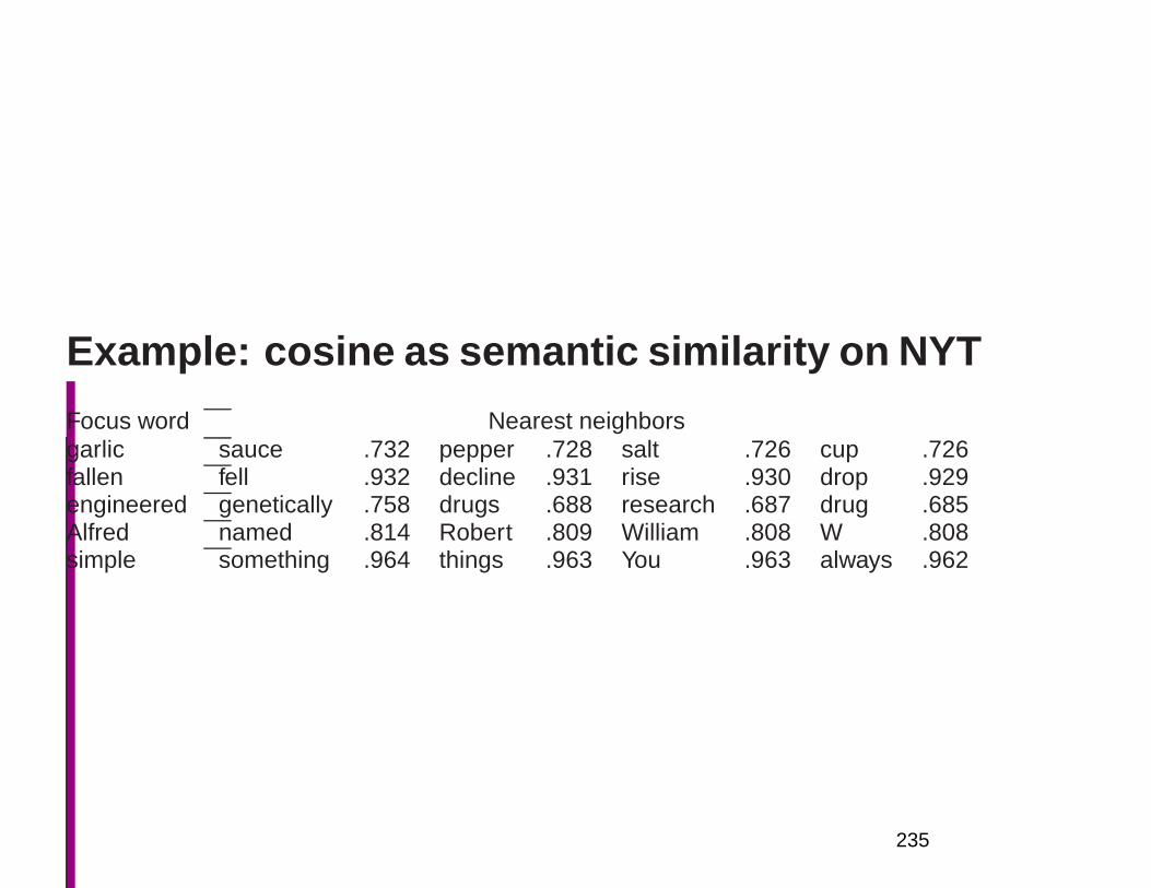
Example: cosine as semantic similarity on NYT
Focus word Nearest neighborsgarlic sauce .732 pepper .728 salt .726 cup .726fallen fell .932 decline .931 rise .930 drop .929engineered genetically .758 drugs .688 research .687 drug .685Alfred named .814 Robert .809 William .808 W .808simple something .964 things .963 You .963 always .962
235
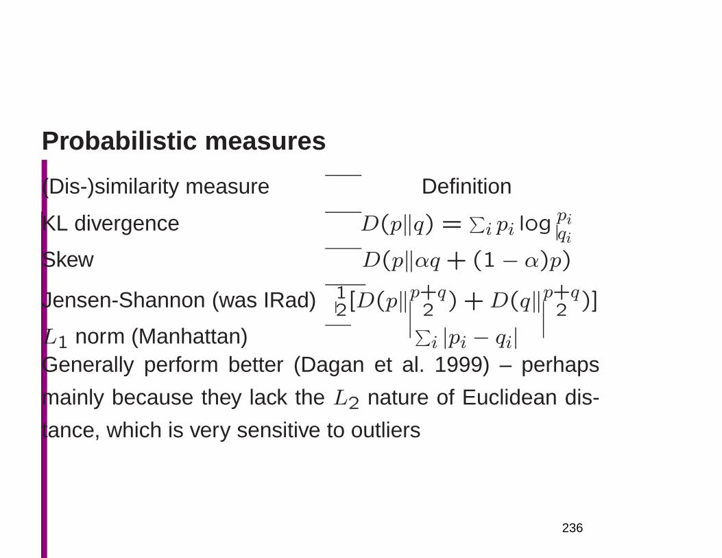
Probabilistic measures
(Dis-)similarity measure Definition
KL divergence D(p‖q) =∑
i pi log piqi
Skew D(p‖αq + (1− α)p)Jensen-Shannon (was IRad) 1
2[D(p‖p+q2 ) +D(q‖p+q
2 )]
L1 norm (Manhattan)∑
i |pi − qi|Generally perform better (Dagan et al. 1999) – perhaps
mainly because they lack the L2 nature of Euclidean dis-
tance, which is very sensitive to outliers
236
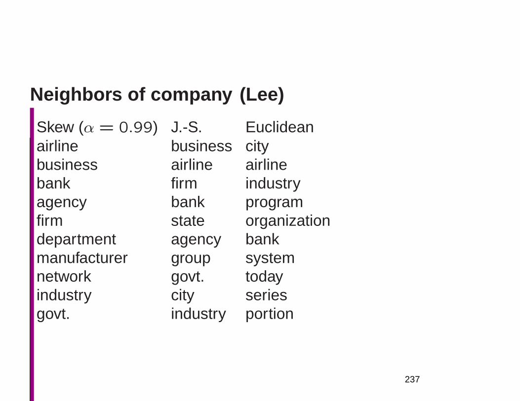
Neighbors of company (Lee)
Skew (α = 0.99) J.-S. Euclideanairline business citybusiness airline airlinebank firm industryagency bank programfirm state organizationdepartment agency bankmanufacturer group systemnetwork govt. todayindustry city seriesgovt. industry portion
237
Evaluation
• Qualitative
• Task-based
– Language models (Dagan, Pereira, and Lee)
– Resnik
– . . .
238
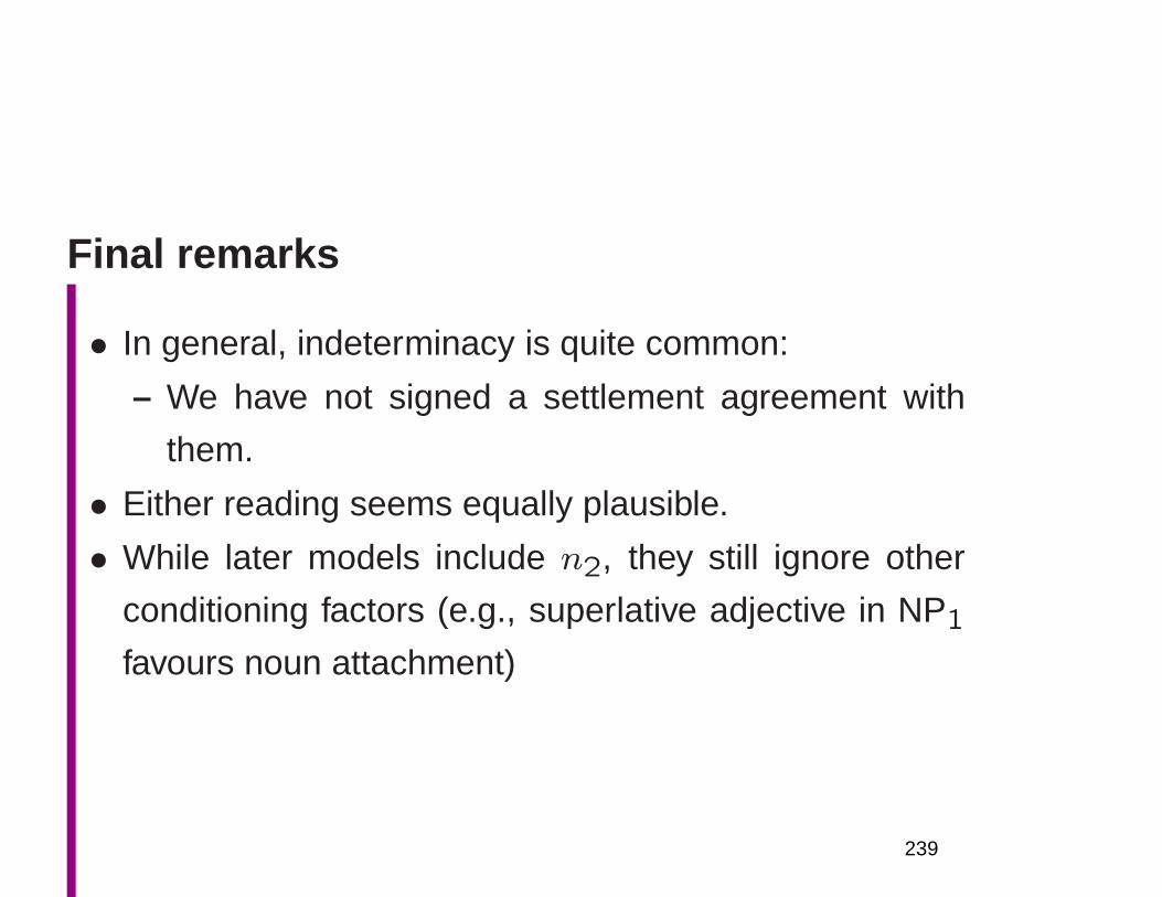
Final remarks
• In general, indeterminacy is quite common:
– We have not signed a settlement agreement with
them.
• Either reading seems equally plausible.
• While later models include n2, they still ignore other
conditioning factors (e.g., superlative adjective in NP1
favours noun attachment)
239
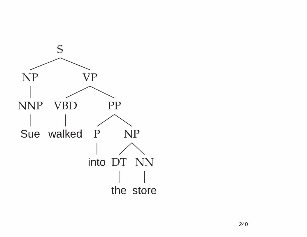
S
NP
NNP
Sue
VP
VBD
walked
PP
P
into
NP
DT
the
NN
store
240

To Do
• In the forward probability, it used to be bjot but it seems
you want i. Need to update the later cases that show
the lattice calculations.
• Also, the slide for β probabilities still has a T + 1 in it,
but it seems like you might as well stop at T .
• Discuss in slide state emission vs. arc emission HMMs
• Implement and work through students paying attention
or not.
241

Part of Speech Tagging
FSNLP, chapters 9 and 10
Christopher Manning andHinrich Schütze
© 1999–2003
242
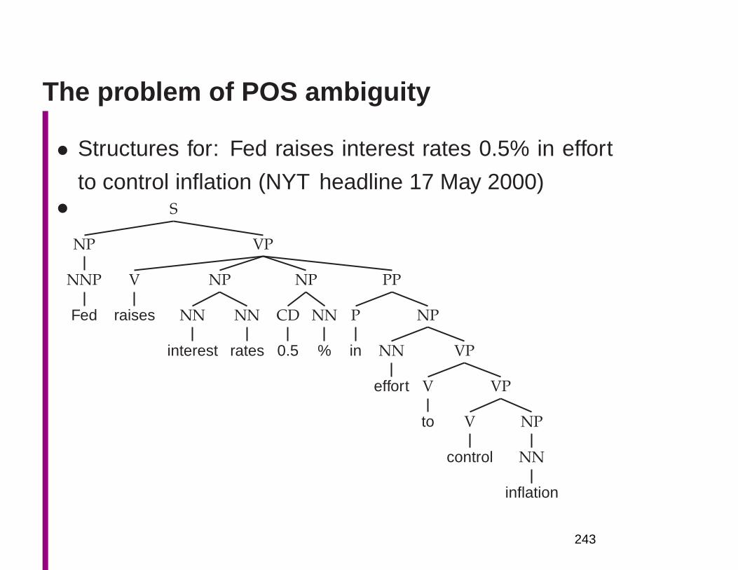
The problem of POS ambiguity
• Structures for: Fed raises interest rates 0.5% in effort
to control inflation (NYT headline 17 May 2000)• S
NP
NNP
Fed
VP
V
raises
NP
NN
interest
NN
rates
NP
CD
0.5
NN
%
PP
P
in
NP
NN
effort
VP
V
to
VP
V
control
NP
NN
inflation
243
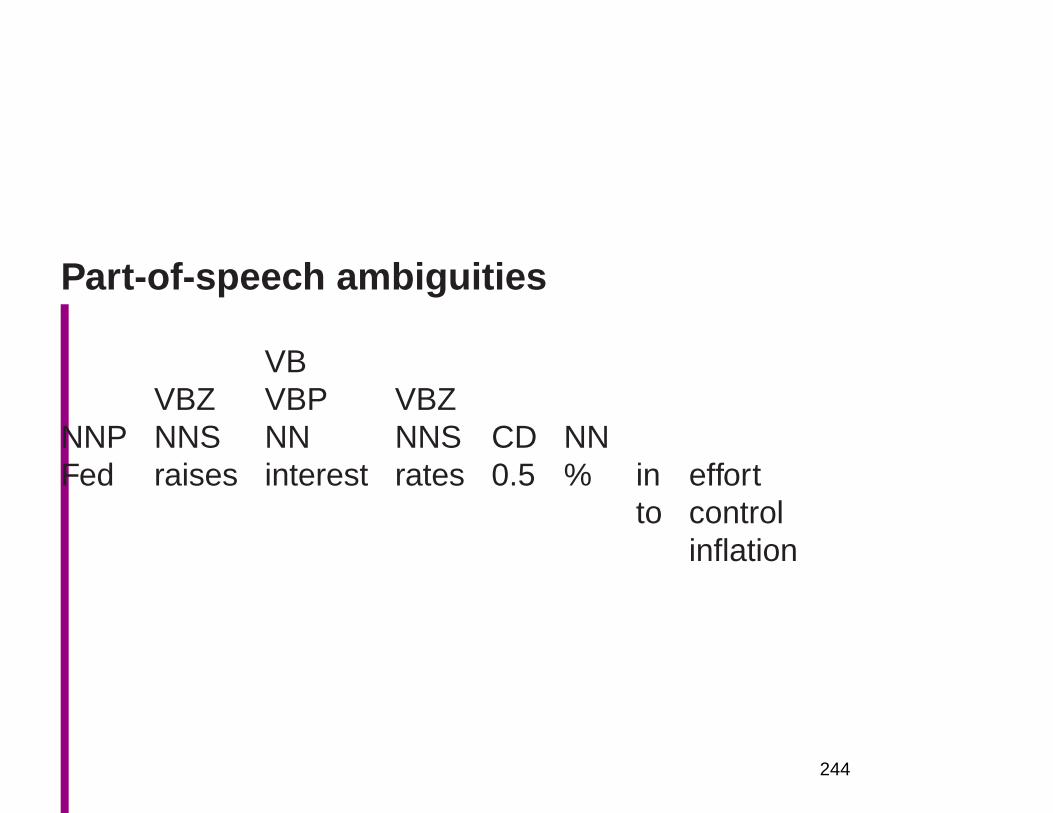
Part-of-speech ambiguities
VBVBZ VBP VBZ
NNP NNS NN NNS CD NNFed raises interest rates 0.5 % in effort
to controlinflation
244
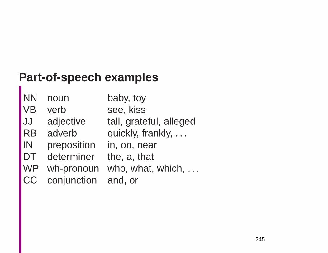
Part-of-speech examples
NN noun baby, toyVB verb see, kissJJ adjective tall, grateful, allegedRB adverb quickly, frankly, . . .IN preposition in, on, nearDT determiner the, a, thatWP wh-pronoun who, what, which, . . .CC conjunction and, or
245
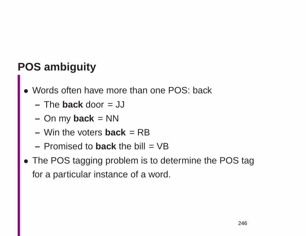
POS ambiguity
• Words often have more than one POS: back
– The back door = JJ
– On my back = NN
– Win the voters back = RB
– Promised to back the bill = VB
• The POS tagging problem is to determine the POS tag
for a particular instance of a word.
246
POS Tagging Applications
• Text-to-speech (how do we pronounce “lead”?)
• WSD if the senses are actually different parts of speech. . .
• Information source in all sorts of tasks such as informa-tion extraction
• All sorts of simple parsing applications: can write reg-exps like Det Adj* N* over the output (e.g., subcatego-rization frame learner)
• Preprocessing to speed up a full parser (but a littledangerous)
• If you know the tag, you can back off to it in other tasks,such as parsing (back-off: use a simpler representationwith denser statistics)
247
Why should we care?
• The first statistical NLP task
• Been done to death by different methods
• Easy to evaluate (how many tags are correct?)
• Canonical sequence (finite-state model) task
• Can be done well with methods that look at local con-
text
• Though should “really” do it by parsing!
• Fast linear task of considerable value
248
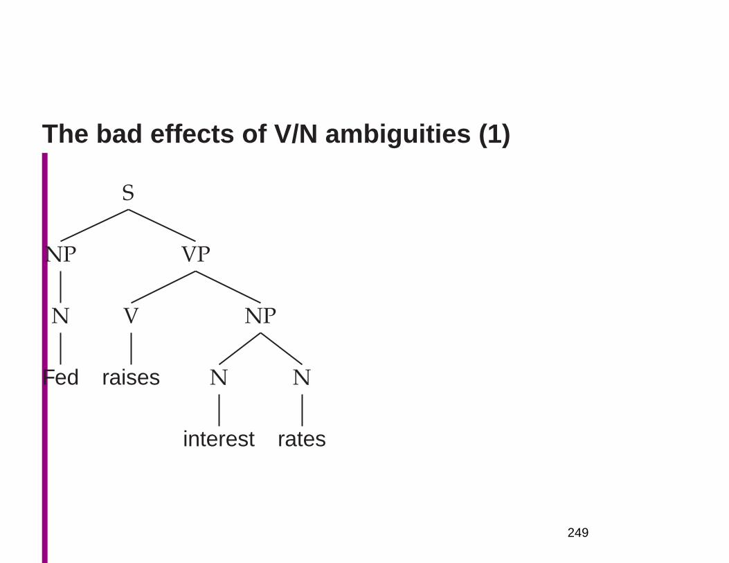
The bad effects of V/N ambiguities (1)
S
NP
N
Fed
VP
V
raises
NP
N
interest
N
rates
249
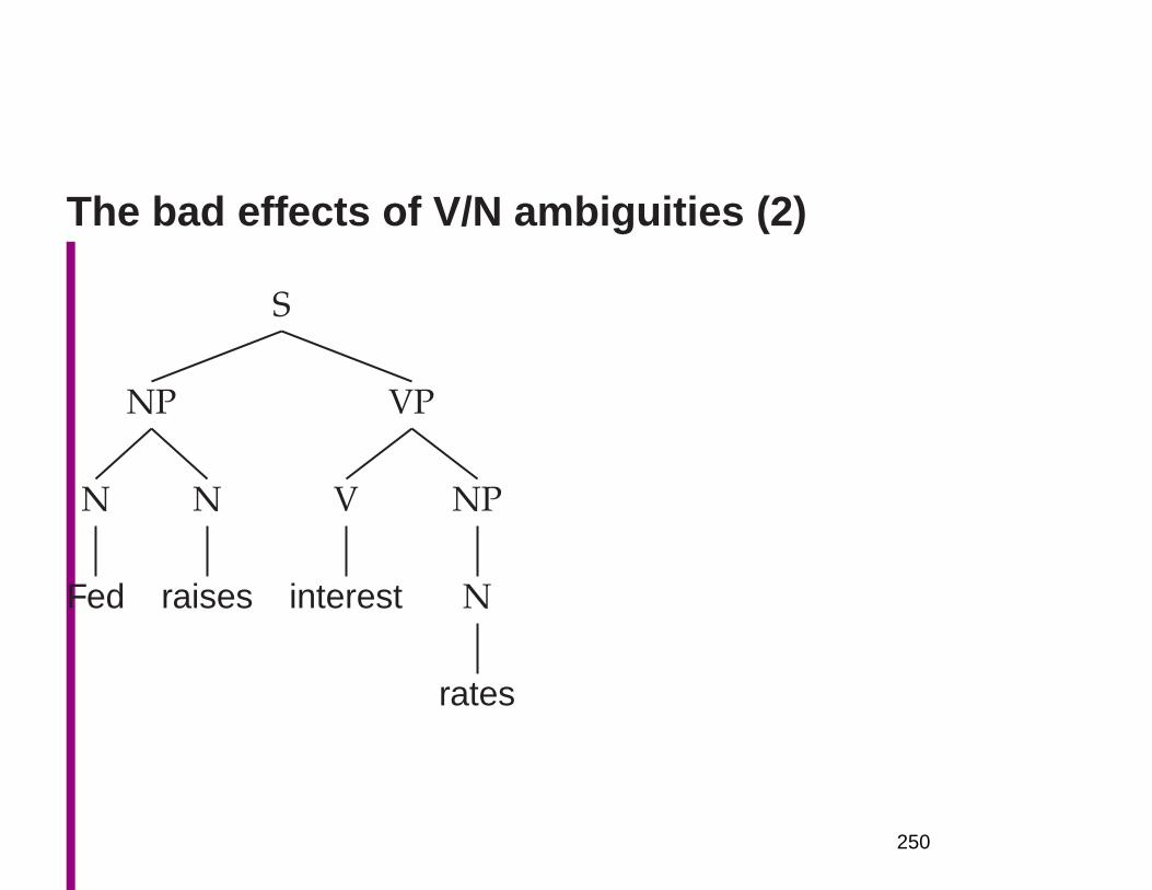
The bad effects of V/N ambiguities (2)
S
NP
N
Fed
N
raises
VP
V
interest
NP
N
rates
250
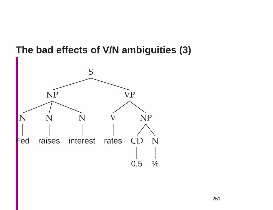
The bad effects of V/N ambiguities (3)
S
NP
N
Fed
N
raises
N
interest
VP
V
rates
NP
CD
0.5
N
%
251
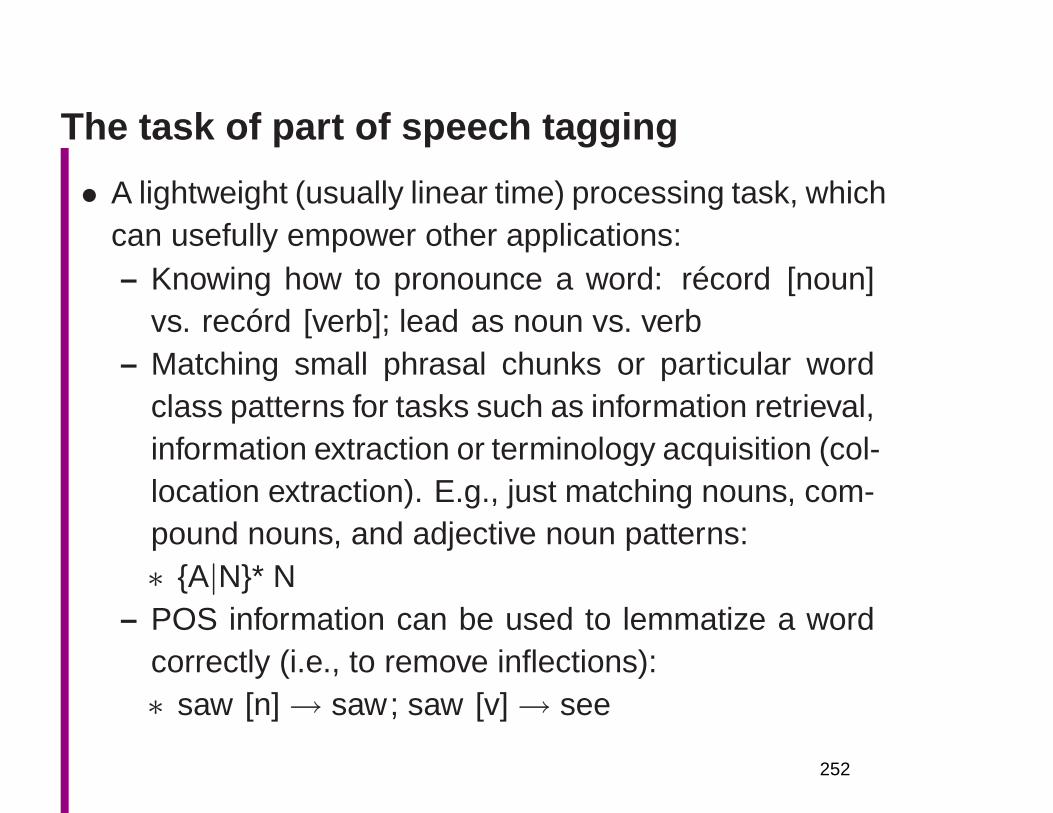
The task of part of speech tagging
• A lightweight (usually linear time) processing task, whichcan usefully empower other applications:– Knowing how to pronounce a word: récord [noun]
vs. recórd [verb]; lead as noun vs. verb– Matching small phrasal chunks or particular word
class patterns for tasks such as information retrieval,information extraction or terminology acquisition (col-location extraction). E.g., just matching nouns, com-pound nouns, and adjective noun patterns:∗ A|N* N
– POS information can be used to lemmatize a wordcorrectly (i.e., to remove inflections):∗ saw [n]→ saw ; saw [v]→ see
252
The task of part of speech tagging
• – Can differentiate word senses that involve part of
speech differences
– POS can be used as backoff in various class-based
models, when too little information is known about a
particular word
– Can be a preprocessor for a parser (speeds up parser;
often better, but more expensive, to let the parser do
the tagging as well)
– Tagged text helps linguists find interesting syntactic
constructions in texts (ssh used as a verb)
253
The linguistics of parts of speech and tag sets
• We’re not going to substantively discuss parts of speech
in class
– Read section 3.1 to learn about parts of speech, par-
ticularly the kind of richer sets of distinctions com-
monly made by linguists and in NLP applications
– Read section 4.3.2 for discussion of POS tag sets
used in NLP.
∗ There’s a handy table explaining tag abbreviations
on pp. 141–142
254

Part of speech tagging
Information sources:
• Sequence of words: syntagmatic information
– Surprisingly weak information source
– Many words have various parts of speech – cf. the
example above
• Frequency of use of words
– Surprisingly effective: gets 90+% performance by
itself (for English)∗
∗ This acts as a baseline for performance
∗Even up to 93.7%, based on the results of Toutanova et al. (2003).
255
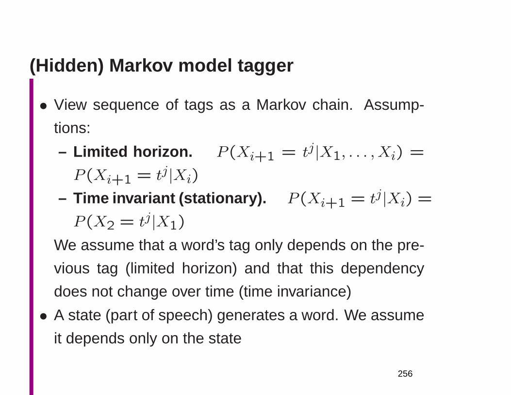
(Hidden) Markov model tagger
• View sequence of tags as a Markov chain. Assump-
tions:
– Limited horizon. P (Xi+1 = tj|X1, . . . , Xi) =
P (Xi+1 = tj|Xi)– Time invariant (stationary). P (Xi+1 = tj|Xi) =
P (X2 = tj|X1)
We assume that a word’s tag only depends on the pre-
vious tag (limited horizon) and that this dependency
does not change over time (time invariance)
• A state (part of speech) generates a word. We assume
it depends only on the state
256
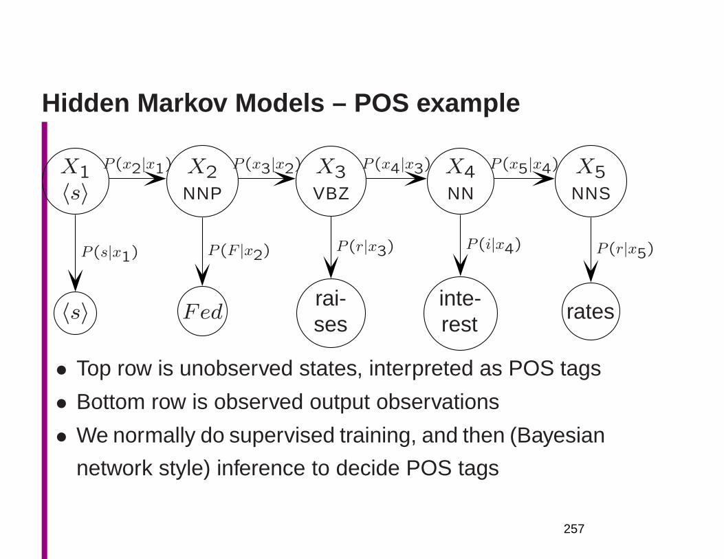
Hidden Markov Models – POS example
X1〈s〉
X2NNP
X3VBZ
X4NN
X5NNS
〈s〉 Fedrai-ses
inte-rest
rates
P (x2|x1) P (x3|x2) P (x4|x3) P (x5|x4)
P (s|x1) P (F |x2) P (r|x3) P (i|x4) P (r|x5)
• Top row is unobserved states, interpreted as POS tags
• Bottom row is observed output observations
• We normally do supervised training, and then (Bayesian
network style) inference to decide POS tags
257
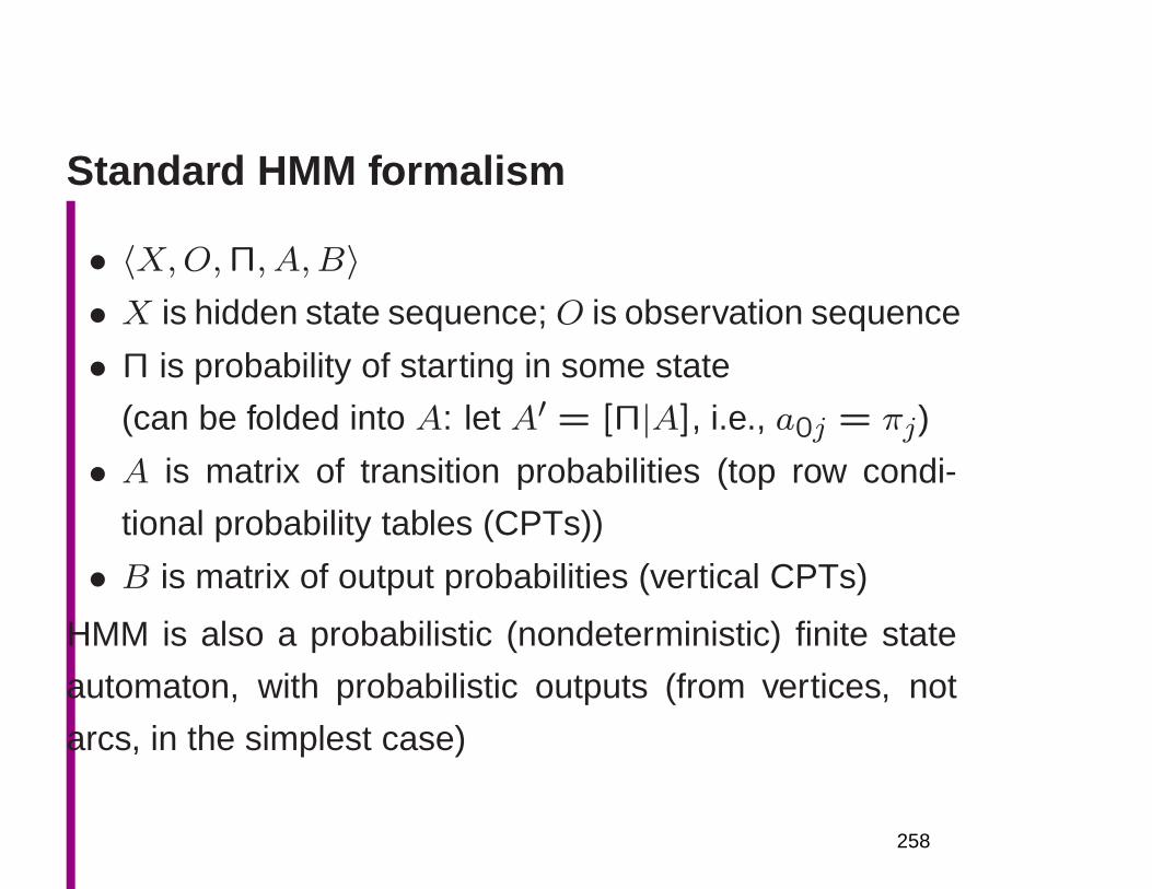
Standard HMM formalism
• 〈X,O,Π, A,B〉• X is hidden state sequence; O is observation sequence
• Π is probability of starting in some state
(can be folded into A: let A′ = [Π|A], i.e., a0j = πj)
• A is matrix of transition probabilities (top row condi-
tional probability tables (CPTs))
• B is matrix of output probabilities (vertical CPTs)
HMM is also a probabilistic (nondeterministic) finite state
automaton, with probabilistic outputs (from vertices, not
arcs, in the simplest case)
258
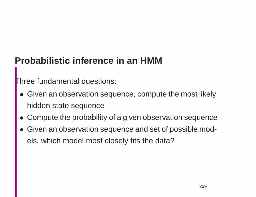
Probabilistic inference in an HMM
Three fundamental questions:
• Given an observation sequence, compute the most likely
hidden state sequence
• Compute the probability of a given observation sequence
• Given an observation sequence and set of possible mod-
els, which model most closely fits the data?
259
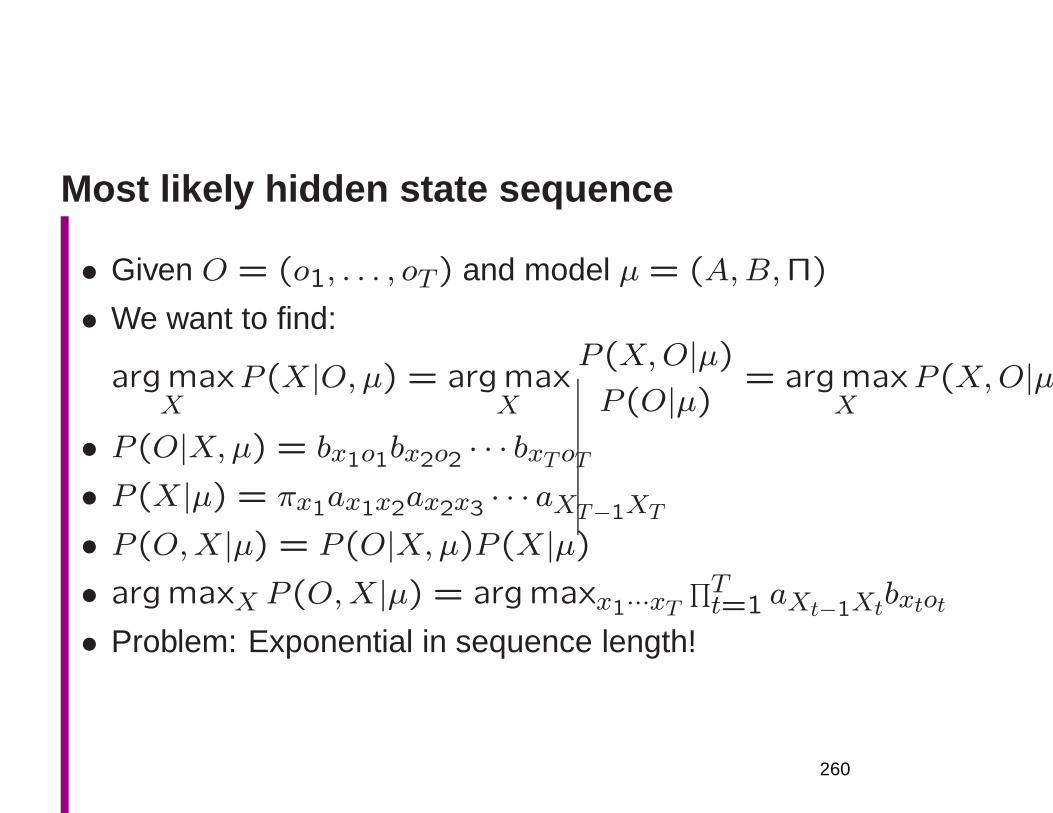
Most likely hidden state sequence
• Given O = (o1, . . . , oT) and model µ = (A,B,Π)
• We want to find:
argmaxX
P (X|O, µ) = argmaxX
P (X,O|µ)P (O|µ) = argmax
XP (X,O|µ)
• P (O|X,µ) = bx1o1bx2o2 · · · bxToT• P (X|µ) = πx1ax1x2ax2x3 · · · aXT−1XT
• P (O,X|µ) = P (O|X,µ)P (X|µ)• argmaxX P (O,X|µ) = argmaxx1···xT
∏Tt=1 aXt−1Xtbxtot
• Problem: Exponential in sequence length!
260
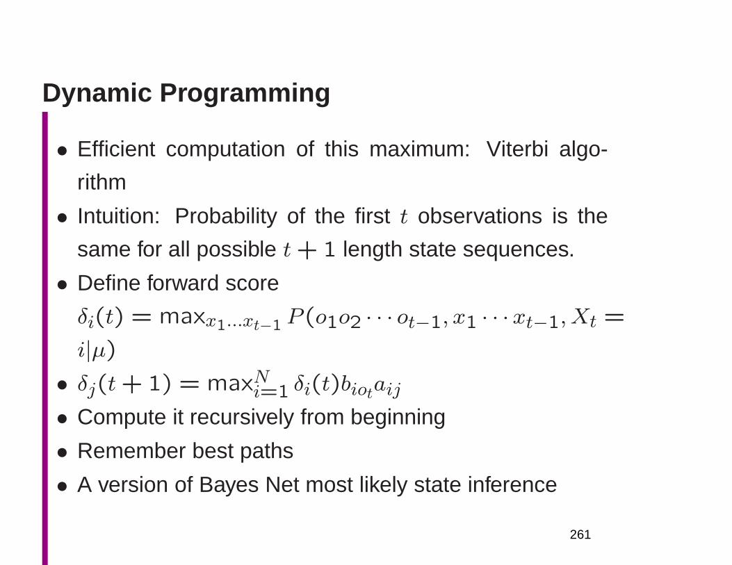
Dynamic Programming
• Efficient computation of this maximum: Viterbi algo-
rithm
• Intuition: Probability of the first t observations is the
same for all possible t+ 1 length state sequences.
• Define forward score
δi(t) = maxx1...xt−1 P (o1o2 · · · ot−1, x1 · · ·xt−1,Xt =
i|µ)• δj(t+ 1) = maxNi=1 δi(t)biotaij
• Compute it recursively from beginning
• Remember best paths
• A version of Bayes Net most likely state inference
261
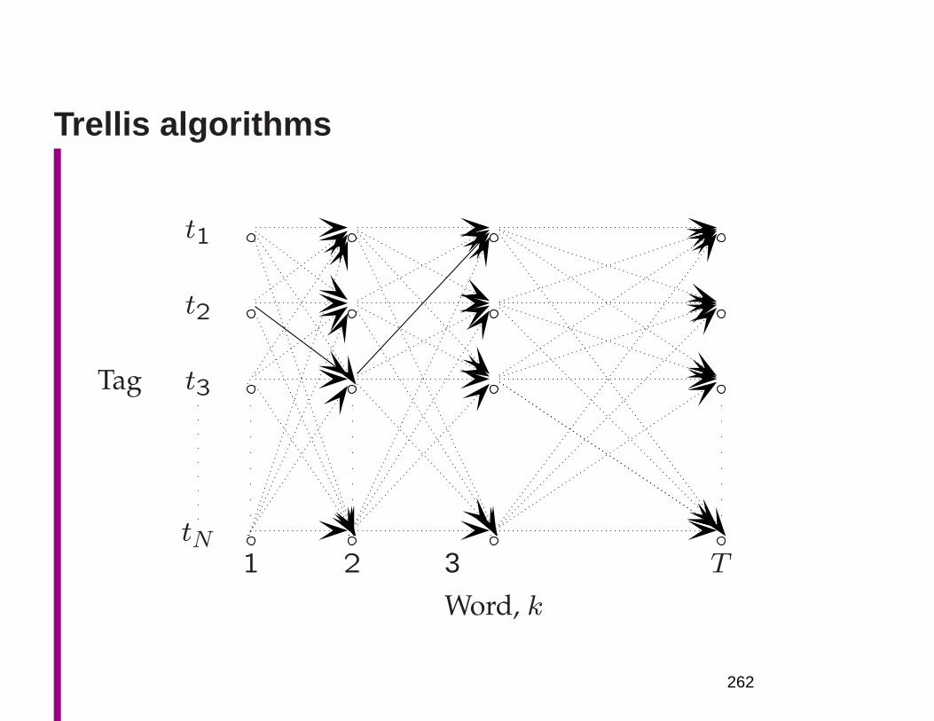
Trellis algorithms
t1
t2
Tag t3
tN1 2 3
Word, k
T
262
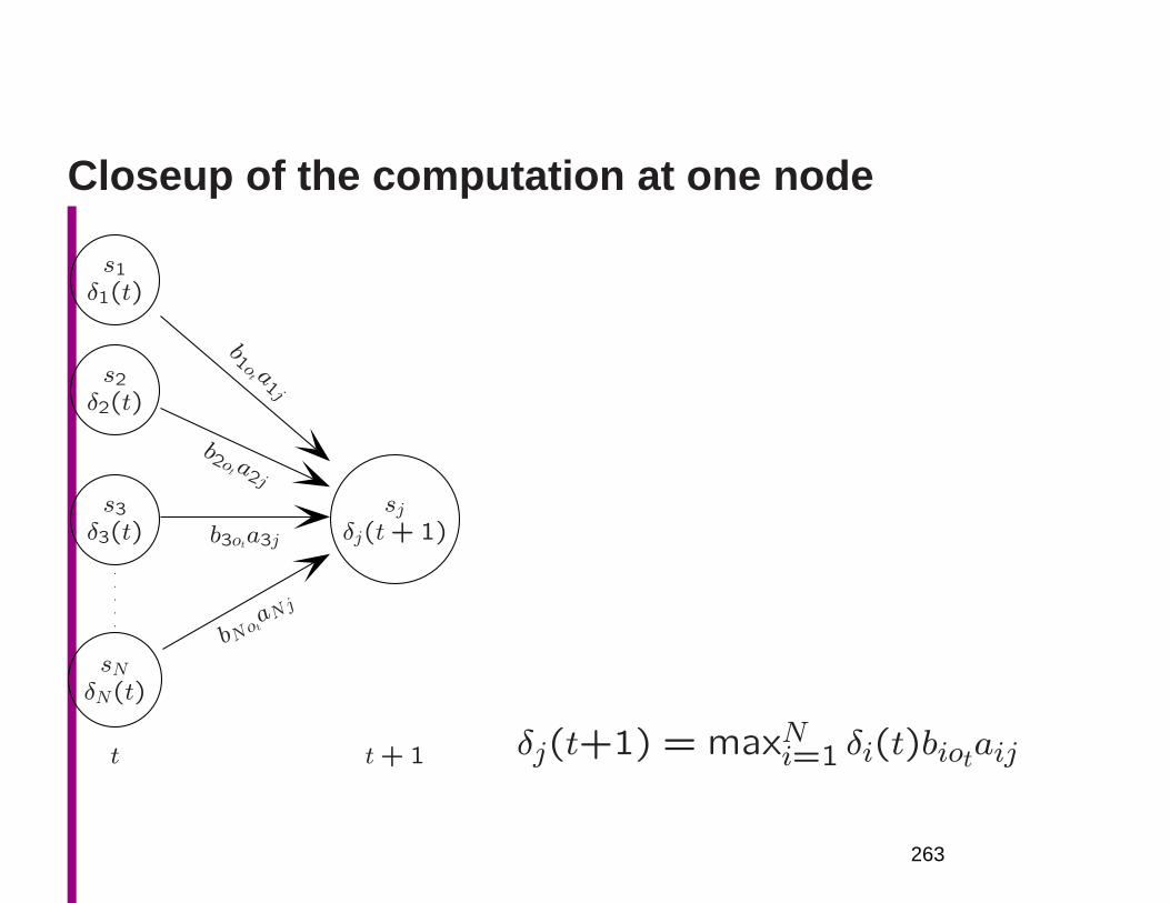
Closeup of the computation at one node
s1δ1(t)
s2δ2(t)
s3δ3(t)
sjδj(t+ 1)
sNδN(t)
t t+ 1
b1ot a
1j
b2ota2j
b3ota3j
bNotaNj
δj(t+1) = maxNi=1 δi(t)biotaij
263
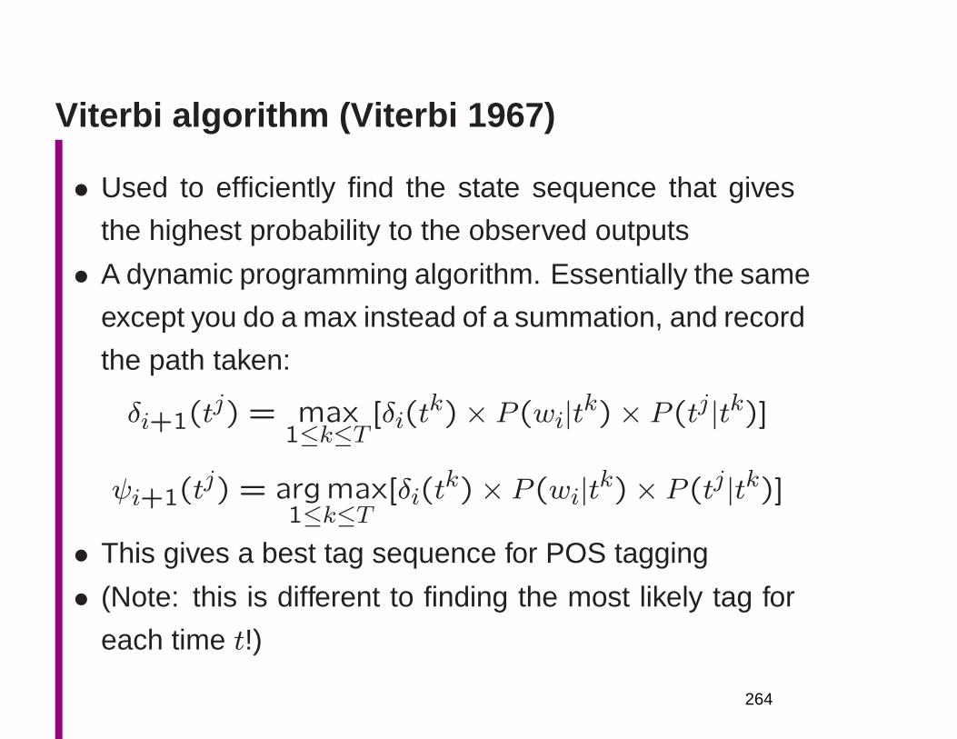
Viterbi algorithm (Viterbi 1967)
• Used to efficiently find the state sequence that gives
the highest probability to the observed outputs
• A dynamic programming algorithm. Essentially the same
except you do a max instead of a summation, and record
the path taken:
δi+1(tj) = max
1≤k≤T[δi(t
k)× P (wi|tk)× P (tj|tk)]
ψi+1(tj) = argmax
1≤k≤T[δi(t
k)× P (wi|tk)× P (tj|tk)]
• This gives a best tag sequence for POS tagging
• (Note: this is different to finding the most likely tag for
each time t!)
264
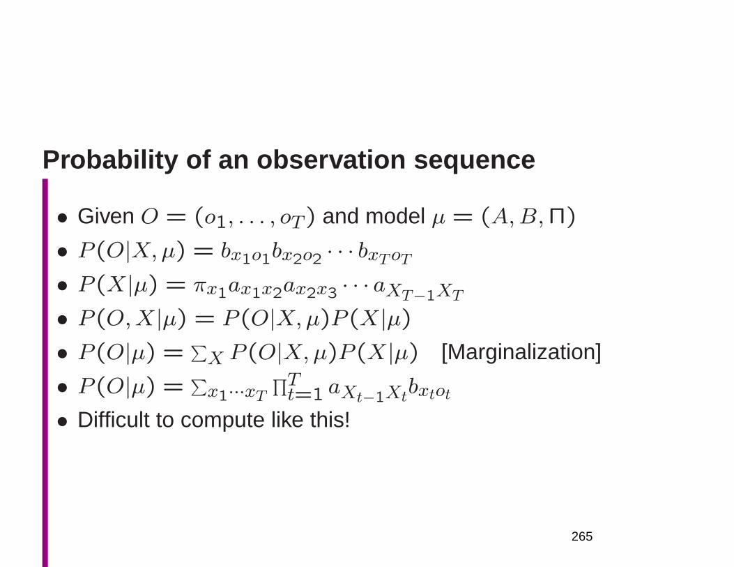
Probability of an observation sequence
• Given O = (o1, . . . , oT) and model µ = (A,B,Π)
• P (O|X,µ) = bx1o1bx2o2 · · · bxToT• P (X|µ) = πx1ax1x2ax2x3 · · · aXT−1XT
• P (O,X|µ) = P (O|X,µ)P (X|µ)• P (O|µ) =
∑
X P (O|X,µ)P (X|µ) [Marginalization]
• P (O|µ) =∑
x1···xT∏Tt=1 aXt−1Xtbxtot
• Difficult to compute like this!
265
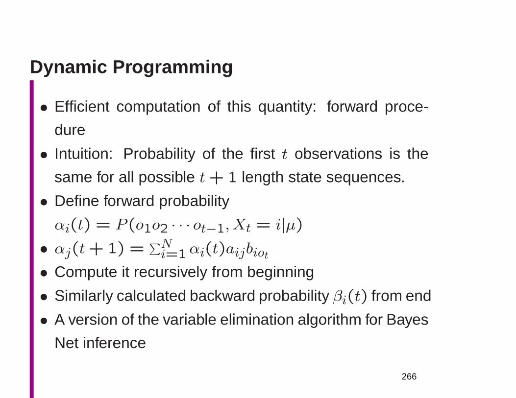
Dynamic Programming
• Efficient computation of this quantity: forward proce-
dure
• Intuition: Probability of the first t observations is the
same for all possible t+ 1 length state sequences.
• Define forward probability
αi(t) = P (o1o2 · · · ot−1, Xt = i|µ)• αj(t+ 1) =
∑Ni=1αi(t)aijbiot
• Compute it recursively from beginning
• Similarly calculated backward probability βi(t) from end
• A version of the variable elimination algorithm for Bayes
Net inference
266
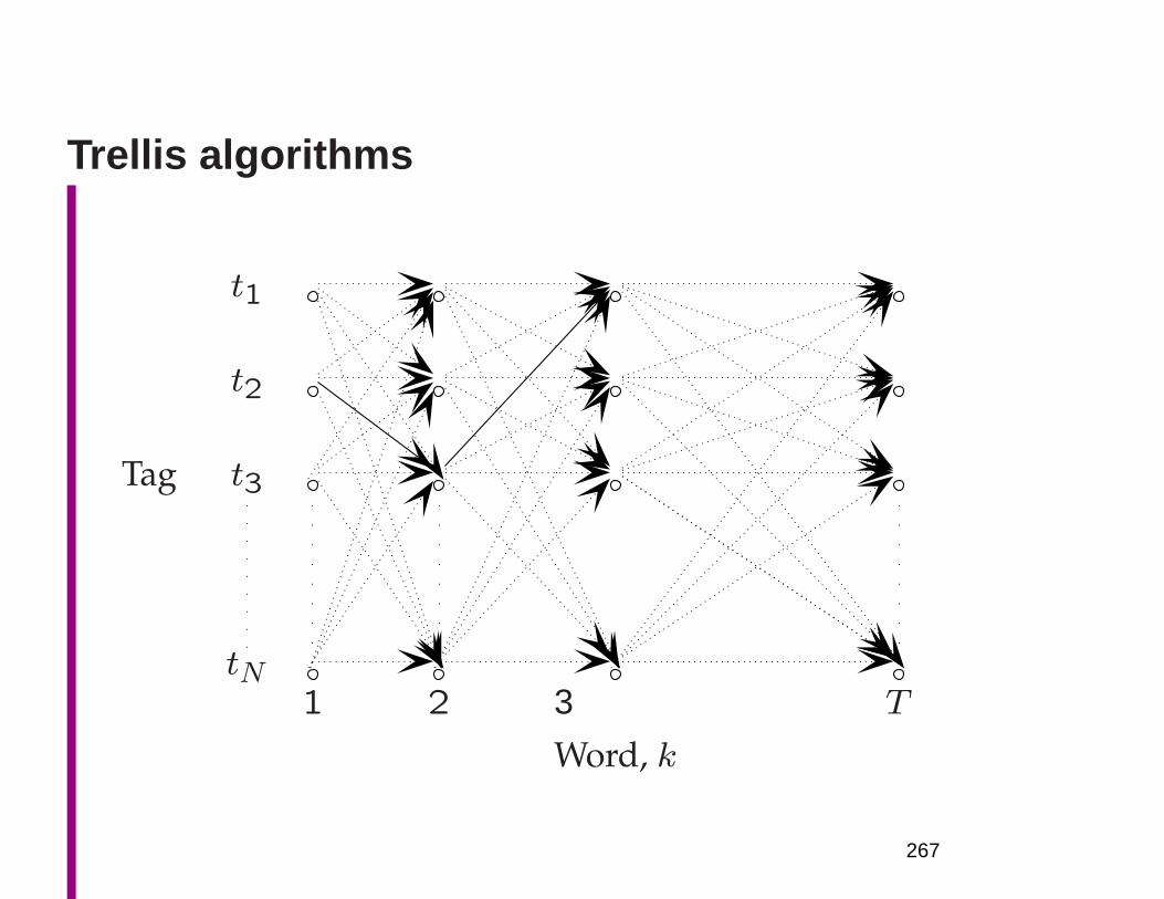
Trellis algorithms
t1
t2
Tag t3
tN1 2 3
Word, k
T
267

Closeup of the computation at one node
s1α1(t)
s2α2(t)
s3α3(t)
sjαj(t+ 1)
sNαN(t)
t t+ 1
a1j bjot
a2jbjo
t
a3jbjot
aNjbj
ot
αj(t+1) =∑Ni=1αi(t)aijbjot
268
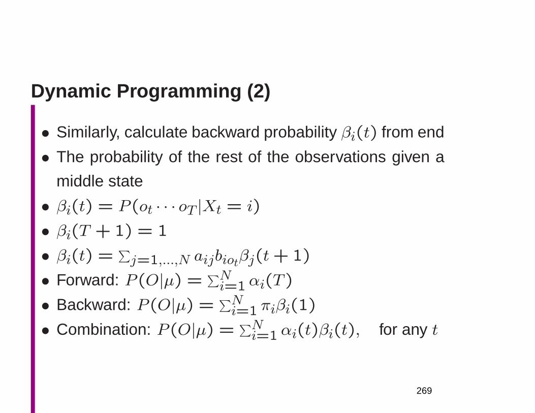
Dynamic Programming (2)
• Similarly, calculate backward probability βi(t) from end
• The probability of the rest of the observations given a
middle state
• βi(t) = P (ot · · · oT |Xt = i)
• βi(T + 1) = 1
• βi(t) =∑
j=1,...,N aijbiotβj(t+ 1)
• Forward: P (O|µ) =∑Ni=1αi(T )
• Backward: P (O|µ) =∑Ni=1 πiβi(1)
• Combination: P (O|µ) =∑Ni=1αi(t)βi(t), for any t
269
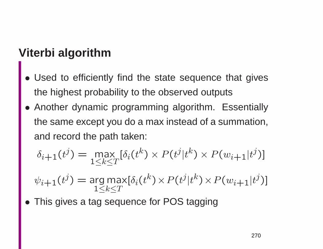
Viterbi algorithm
• Used to efficiently find the state sequence that gives
the highest probability to the observed outputs
• Another dynamic programming algorithm. Essentially
the same except you do a max instead of a summation,
and record the path taken:
δi+1(tj) = max
1≤k≤T[δi(t
k)× P (tj|tk)× P (wi+1|tj)]
ψi+1(tj) = argmax
1≤k≤T[δi(t
k)×P (tj|tk)×P (wi+1|tj)]
• This gives a tag sequence for POS tagging
270
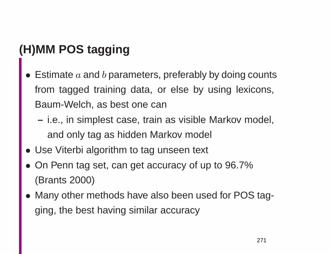
(H)MM POS tagging
• Estimate a and b parameters, preferably by doing counts
from tagged training data, or else by using lexicons,
Baum-Welch, as best one can
– i.e., in simplest case, train as visible Markov model,
and only tag as hidden Markov model
• Use Viterbi algorithm to tag unseen text
• On Penn tag set, can get accuracy of up to 96.7%
(Brants 2000)
• Many other methods have also been used for POS tag-
ging, the best having similar accuracy
271
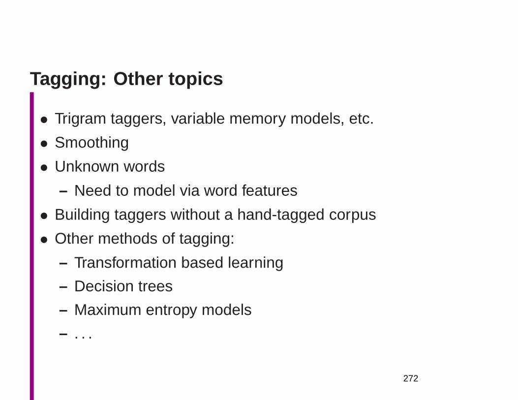
Tagging: Other topics
• Trigram taggers, variable memory models, etc.
• Smoothing
• Unknown words
– Need to model via word features
• Building taggers without a hand-tagged corpus
• Other methods of tagging:
– Transformation based learning
– Decision trees
– Maximum entropy models
– . . .
272
Tagging: Other topics
• Other languages
• Accuracy (factors: training data, tag set, drift, unknown
words)
• You gain by having an explicit end symbol/state (mak-
ing it a probabilistic regular grammar)
• Parameter tying (see following language model exam-
ple)
• Linguistic foundations of tags: not always determinate
• Applications: IR, IE, QA, terminology extraction
273
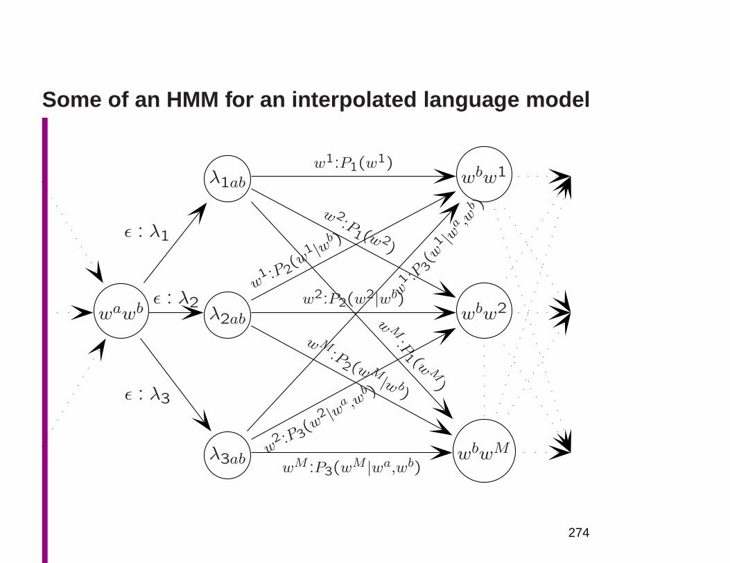
Some of an HMM for an interpolated language model
λ1ab wbw1
wawb λ2ab wbw2
λ3ab wbwM
ǫ : λ1
ǫ : λ2
ǫ : λ3
w1:P1(w1)
w 2:P
1(w 2)
w M:P
1 (w M)
w1 :P2
(w1 |w
b )
w2:P2(w2|wb)
wM:P
2(wM|w b
)w
1 :P3(w
1 |wa ,w
b )
w2 :P3
(w2 |w
a ,wb )
wM :P3(wM |wa,wb)
274
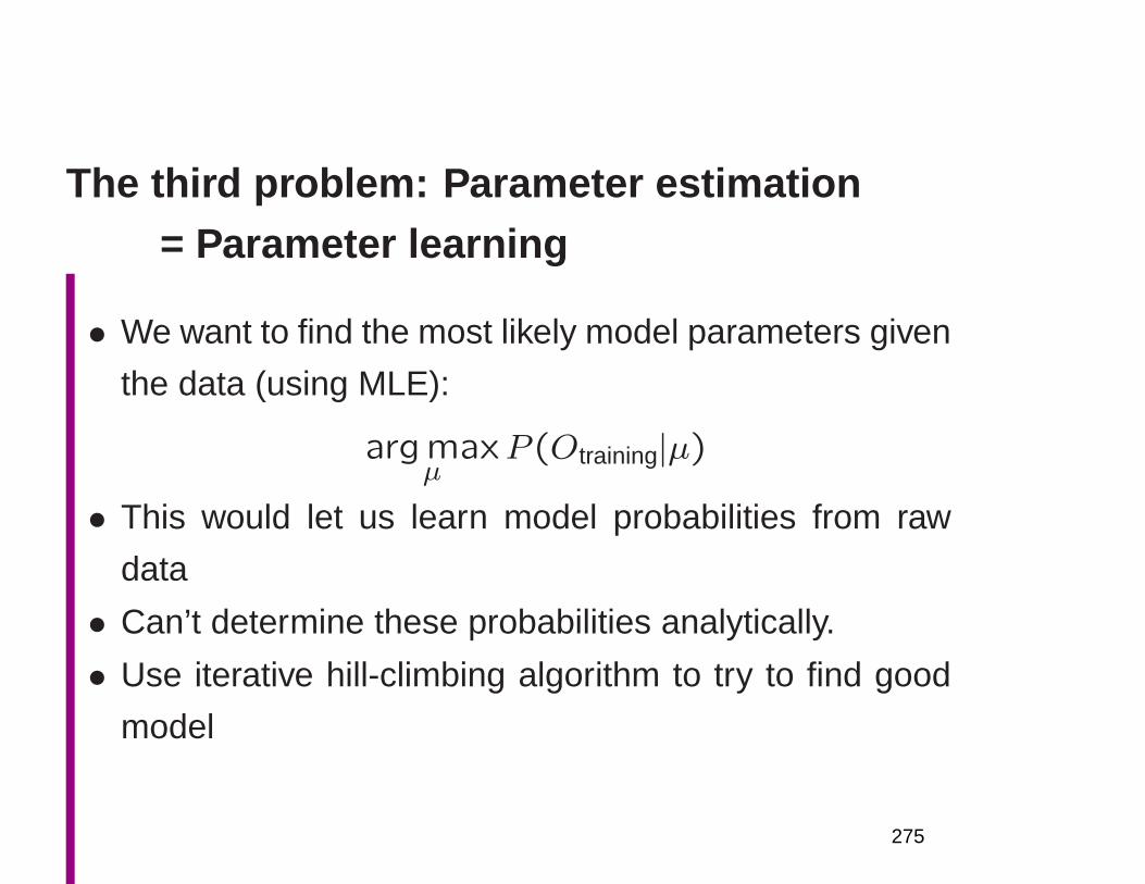
The third problem: Parameter estimation= Parameter learning
• We want to find the most likely model parameters given
the data (using MLE):
argmaxµ
P (Otraining|µ)
• This would let us learn model probabilities from raw
data
• Can’t determine these probabilities analytically.
• Use iterative hill-climbing algorithm to try to find good
model
275
HMM Training: Baum-Welch reestimation
• Used to automatically estimate parameters of an HMM
• a.k.a. the Forward-Backward algorithm
• A case of the Expectation Maximization (EM) algorithm
• One starts with initial probability estimates
• One computes expectations of how often each transi-
tion/emission is used
• One re-estimates the probabilities based on those ex-
pectations
• . . . and repeat until convergence
276

HMM Training: Baum-Welch reestimation
• Needed because the state paths are hidden, and theequations cannot be solved analytically
• Provides a maximum likelihood estimate: attempts tofind the model that assigns the training data the highestlikelihood
• Hill-climbing algorithm that can get stuck in local max-ima
• Not so effective for inductive POS tagging (the ML re-estimation procedure doesn’t know the meaning we havegiven to the hidden states)
• But good in many tasks (speech, including informationextraction)
277
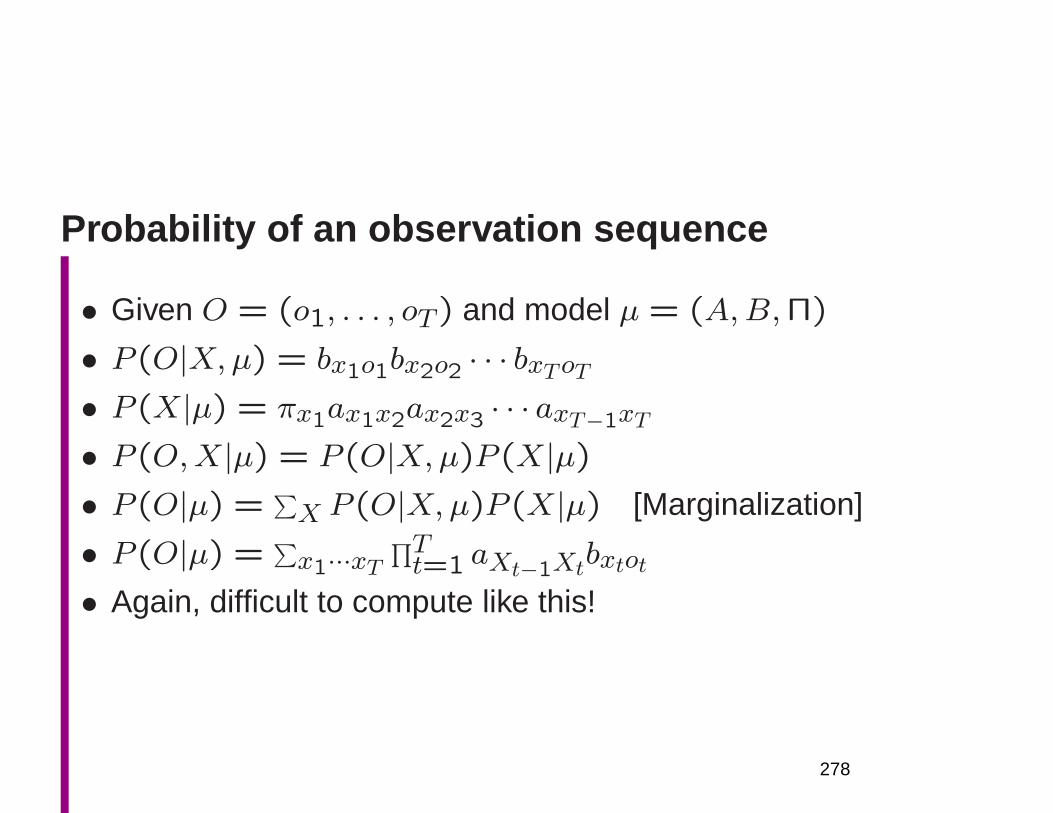
Probability of an observation sequence
• Given O = (o1, . . . , oT) and model µ = (A,B,Π)
• P (O|X,µ) = bx1o1bx2o2 · · · bxToT• P (X|µ) = πx1ax1x2ax2x3 · · · axT−1xT
• P (O,X|µ) = P (O|X,µ)P (X|µ)• P (O|µ) =
∑
X P (O|X,µ)P (X|µ) [Marginalization]
• P (O|µ) =∑
x1···xT∏Tt=1 aXt−1Xtbxtot
• Again, difficult to compute like this!
278
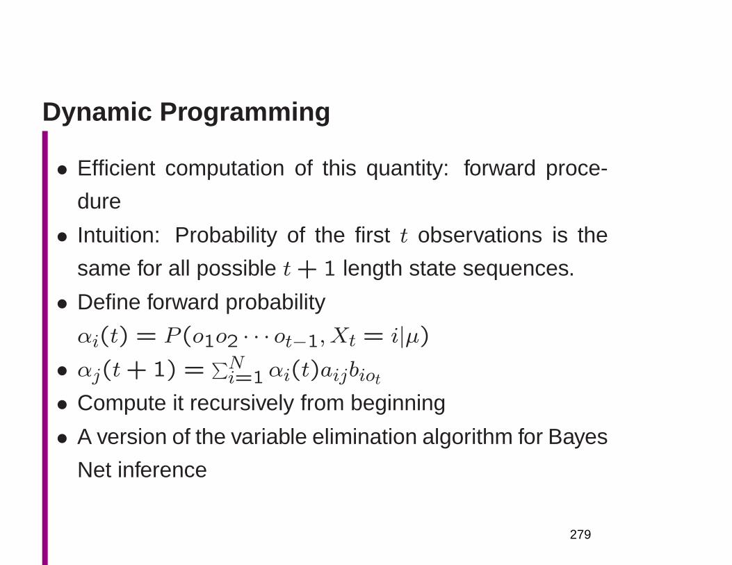
Dynamic Programming
• Efficient computation of this quantity: forward proce-
dure
• Intuition: Probability of the first t observations is the
same for all possible t+ 1 length state sequences.
• Define forward probability
αi(t) = P (o1o2 · · · ot−1, Xt = i|µ)• αj(t+ 1) =
∑Ni=1αi(t)aijbiot
• Compute it recursively from beginning
• A version of the variable elimination algorithm for Bayes
Net inference
279

Closeup of the computation at one node
s1α1(t)
s2α2(t)
s3α3(t)
sjαj(t+ 1)
sNαN(t)
t t+ 1
a1j bjot
a2jbjo
t
a3jbjot
aNjbj
ot
αj(t+1) =∑Ni=1αi(t)aijbjot
280

Dynamic Programming (2)
• Similarly, calculate backward probability βi(t) from end
• The probability of the rest of the observations given a
middle state
• βi(t) = P (ot · · · oT |Xt = i)
• βi(T + 1) = 1
• βi(t) =∑
j=1,...,N aijbiotβj(t+ 1)
• Forward: P (O|µ) =∑Ni=1αi(T )
• Backward: P (O|µ) =∑Ni=1 πiβi(1)
• Combination: P (O|µ) =∑Ni=1αi(t)βi(t), for any t
281
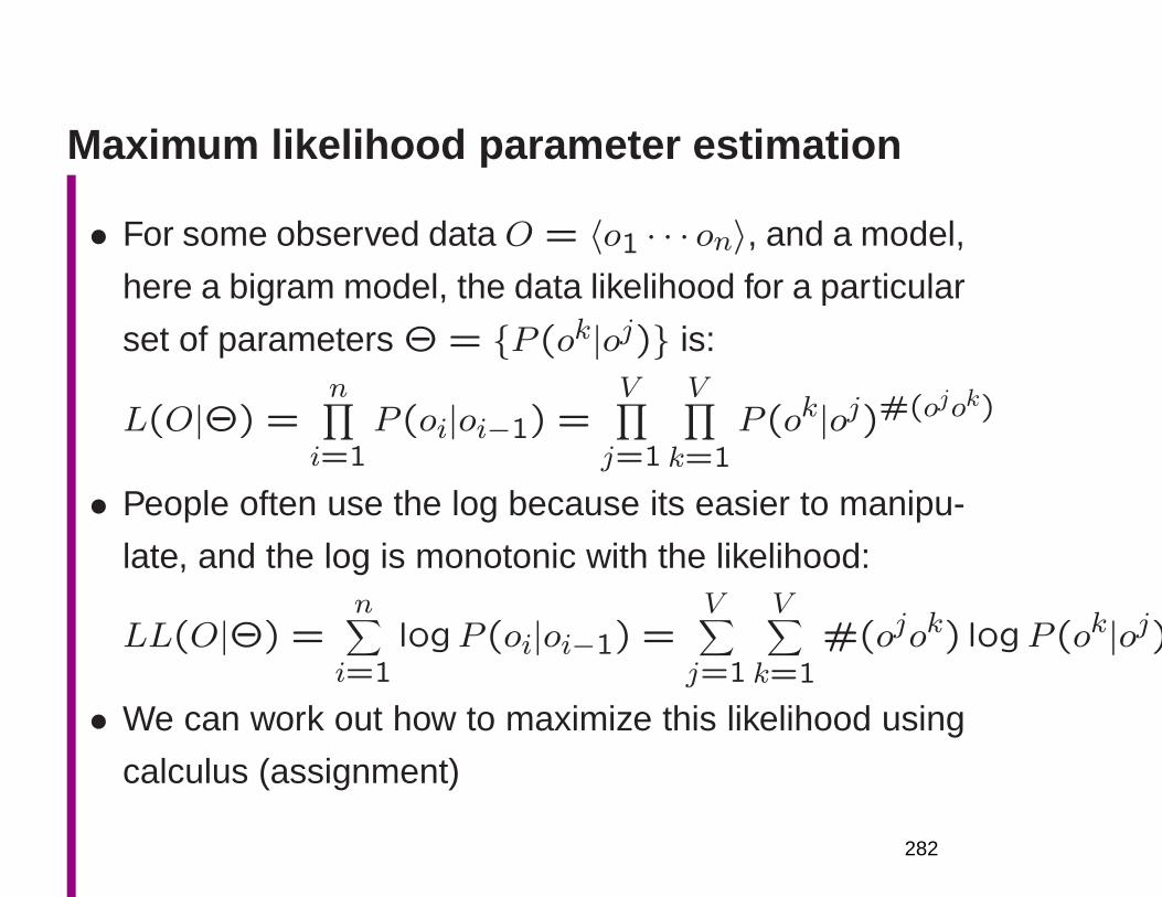
Maximum likelihood parameter estimation
• For some observed data O = 〈o1 · · · on〉, and a model,
here a bigram model, the data likelihood for a particular
set of parameters Θ = P (ok|oj) is:
L(O|Θ) =n∏
i=1P (oi|oi−1) =
V∏
j=1
V∏
k=1
P (ok|oj)#(ojok)
• People often use the log because its easier to manipu-
late, and the log is monotonic with the likelihood:
LL(O|Θ) =n
∑
i=1logP (oi|oi−1) =
V∑
j=1
V∑
k=1
#(ojok) logP (ok|oj)
• We can work out how to maximize this likelihood using
calculus (assignment)
282
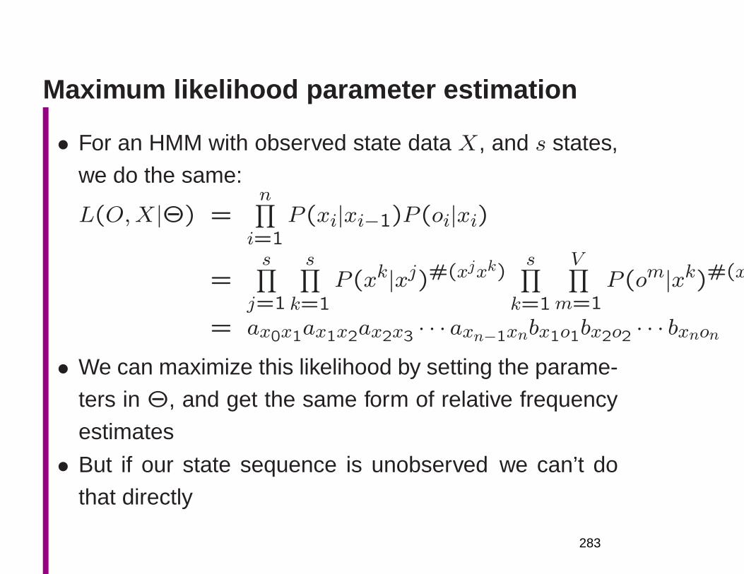
Maximum likelihood parameter estimation
• For an HMM with observed state data X, and s states,
we do the same:
L(O,X|Θ) =n∏
i=1P (xi|xi−1)P (oi|xi)
=s
∏
j=1
s∏
k=1
P (xk|xj)#(xjxk)s
∏
k=1
V∏
m=1P (om|xk)#(x
= ax0x1ax1x2ax2x3 · · · axn−1xnbx1o1bx2o2 · · · bxnon• We can maximize this likelihood by setting the parame-
ters in Θ, and get the same form of relative frequency
estimates
• But if our state sequence is unobserved we can’t do
that directly
283
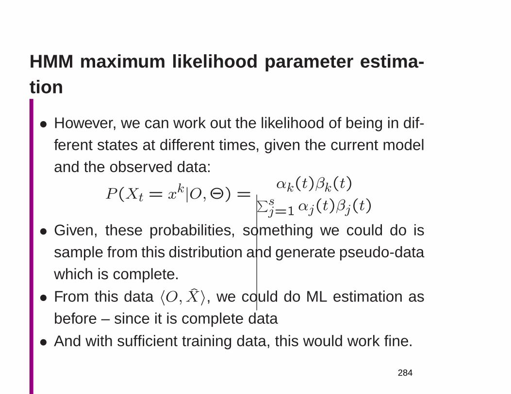
HMM maximum likelihood parameter estima-tion
• However, we can work out the likelihood of being in dif-ferent states at different times, given the current modeland the observed data:
P (Xt = xk|O,Θ) =αk(t)βk(t)
∑sj=1αj(t)βj(t)
• Given, these probabilities, something we could do issample from this distribution and generate pseudo-datawhich is complete.
• From this data 〈O, X〉, we could do ML estimation asbefore – since it is complete data
• And with sufficient training data, this would work fine.
284
HMM maximum likelihood parameter estima-tion
• For the EM algorithm, we do something just slightly
subtler. We work out the expected number of times
we made each state transition and emitted each sym-
bol from each state. This is conceptually just like an
observed count, but it’ll usually be a non-integer
• We then work out new parameter estimates as relative
frequencies just like before.
285
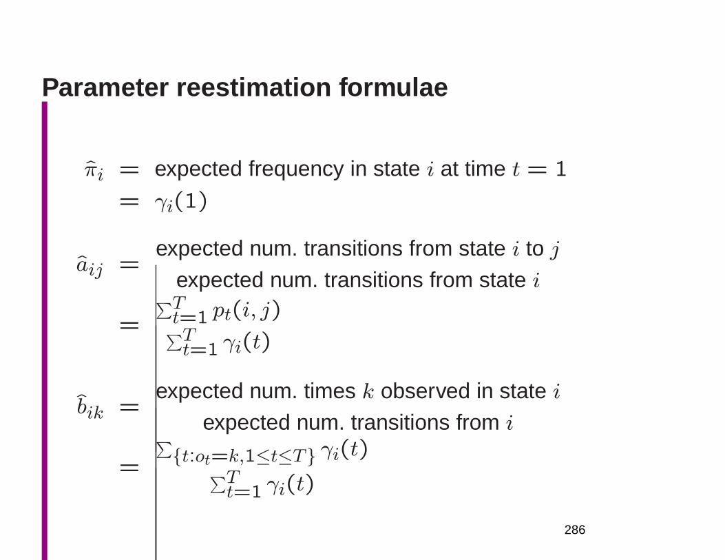
Parameter reestimation formulae
πi = expected frequency in state i at time t = 1
= γi(1)
aij =expected num. transitions from state i to j
expected num. transitions from state i
=
∑Tt=1 pt(i, j)
∑Tt=1 γi(t)
bik =expected num. times k observed in state i
expected num. transitions from i
=
∑
t:ot=k,1≤t≤T γi(t)∑Tt=1 γi(t)
286
EM Algorithm
• Changing the parameters in this way must have in-creased (or at any rate not decreased) the likelihoodof this completion of the data: we’re setting the pa-rameters on the pseudo-observed data to maximize thelikelihood of this pseudo-observed data• But, then, we use these parameter estimates to com-
pute new expectations (or, to sample new completedata)• Since this new data completion is directly based on the
current parameter settings, it is at least intuitively rea-sonable to think that the model should assign it higherlikelihood than the old completion (which was based ondifferent parameter settings)
287
We’re guaranteed to get no worse
• Repeating these two steps iteratively gives us the EM
algorithm
• One can prove rigorously that iterating it changes the
parameters in such a way that the data likelihood is
non-decreasing (Baum et al. 1970; Dempster et al. 1977)
• But we can get stuck in local maxima or on saddle
points, though
– For a lot of NLP problems with a lot of hidden struc-
ture, this is actually a big problem
288
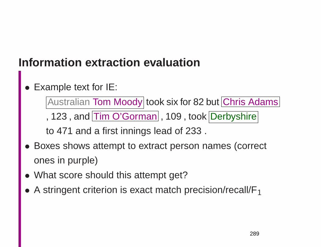
Information extraction evaluation
• Example text for IE:
Australian Tom Moody took six for 82 but Chris Adams
, 123 , and Tim O’Gorman , 109 , took Derbyshire
to 471 and a first innings lead of 233 .
• Boxes shows attempt to extract person names (correct
ones in purple)
• What score should this attempt get?
• A stringent criterion is exact match precision/recall/F1
289

Precision and recall
• Precision is defined as a measure of the proportion of
selected items that the system got right:
precision =tp
tp+ fp
• Recall is defined as the proportion of the target items
that the system selected:
recall =tp
tp+ fn
These two measures allow us to distinguish between ex-
cluding target items and returning irrelevant items.
They still require human-made “gold standard” judgements.
290

Combining them: The F measure
Weighted harmonic mean: The F measure (where F =
1− E):
F =1
α1P + (1− α)1
R
where P is precision, R is recall and α weights precision
and recall. (Or in terms of β, where α = 1/(β2 + 1).)
A value of α = 0.5 is often chosen.
F =2PR
R+ P
At break-even point, when R = P , then F = R = P
291

The F measure ( α = 0.5)
f(x,y)
00.2
0.40.6
0.81 0
0.2
0.4
0.6
0.8
1
00.10.20.30.40.50.60.70.80.9
1
292
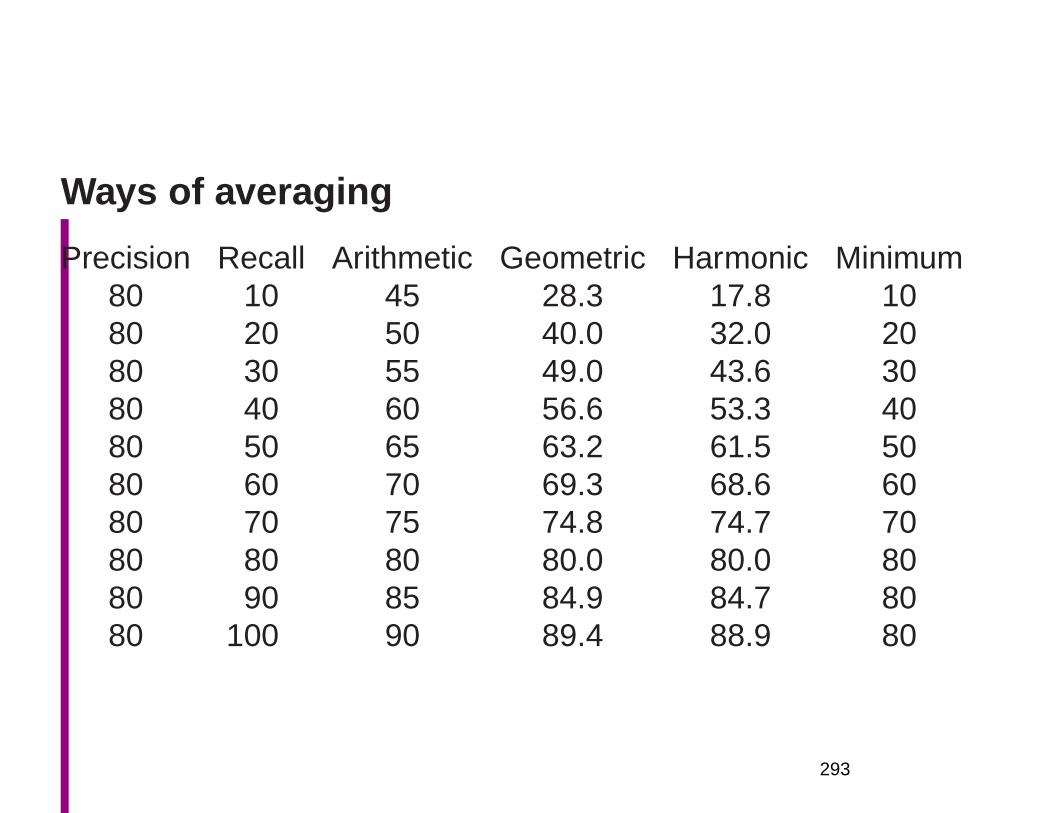
Ways of averaging
Precision Recall Arithmetic Geometric Harmonic Minimum80 10 45 28.3 17.8 1080 20 50 40.0 32.0 2080 30 55 49.0 43.6 3080 40 60 56.6 53.3 4080 50 65 63.2 61.5 5080 60 70 69.3 68.6 6080 70 75 74.8 74.7 7080 80 80 80.0 80.0 8080 90 85 84.9 84.7 8080 100 90 89.4 88.9 80
293
EM Algorithm Intuition
• We don’t know what the model is.
• But we can work out the probability of the observation
sequence using some (perhaps random) model
• Looking at that calculation, we can see which state
transitions and symbol emissions were probably used
the most
• By increasing the probability of those, we can choose
a revised model which gives a higher probability to the
observation sequence
294
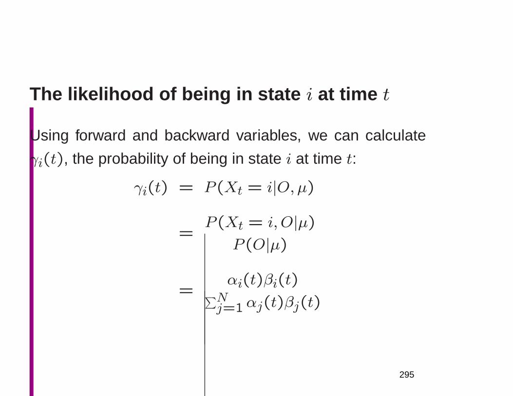
The likelihood of being in state i at time t
Using forward and backward variables, we can calculate
γi(t), the probability of being in state i at time t:
γi(t) = P (Xt = i|O,µ)
=P (Xt = i, O|µ)
P (O|µ)
=αi(t)βi(t)
∑Nj=1αj(t)βj(t)
295
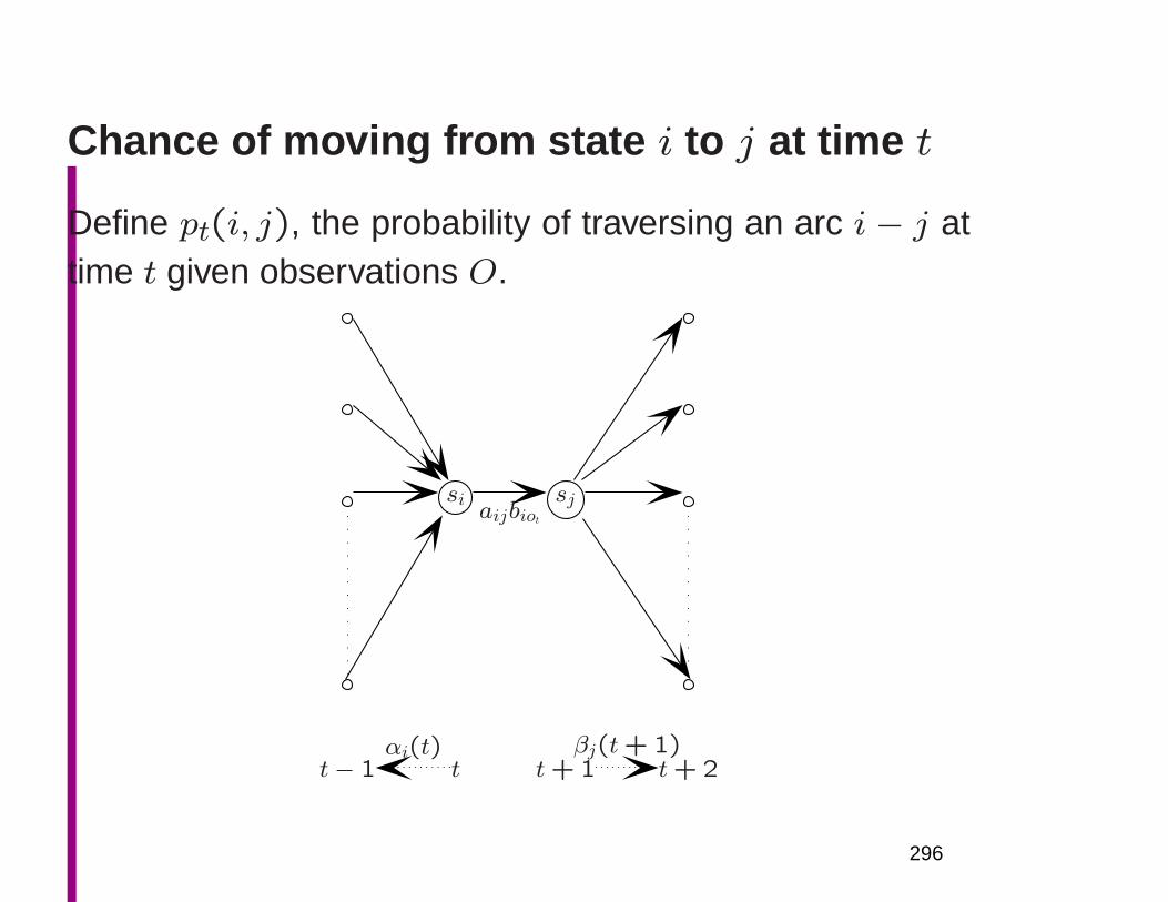
Chance of moving from state i to j at time t
Define pt(i, j), the probability of traversing an arc i − j attime t given observations O.
si sj
t− 1 t t+ 1 t+ 2
aijbiot
αi(t) βj(t+ 1)
296
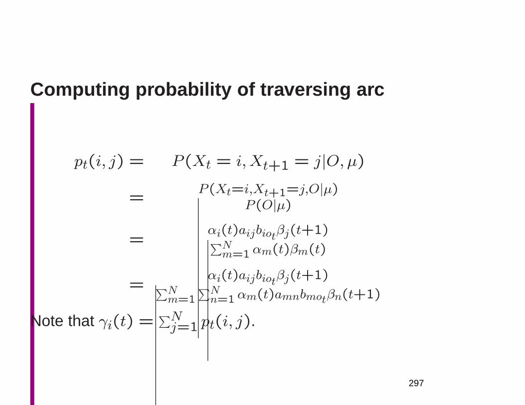
Computing probability of traversing arc
pt(i, j) = P (Xt = i,Xt+1 = j|O, µ)
=P(Xt=i,Xt+1=j,O|µ)
P(O|µ)
=αi(t)aijbiotβj(t+1)∑Nm=1 αm(t)βm(t)
=αi(t)aijbiotβj(t+1)
∑Nm=1
∑Nn=1αm(t)amnbmotβn(t+1)
Note that γi(t) =∑Nj=1 pt(i, j).
297
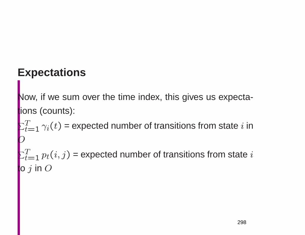
Expectations
Now, if we sum over the time index, this gives us expecta-
tions (counts):∑Tt=1 γi(t) = expected number of transitions from state i in
O∑Tt=1 pt(i, j) = expected number of transitions from state i
to j in O
298

Parameter reestimation formulae
πi = expected frequency in state i at time t = 1
= γi(1)
aij =expected num. transitions from state i to j
expected num. transitions from state i
=
∑Tt=1 pt(i, j)
∑Tt=1 γi(t)
bik =expected num. times k observed in state i
expected num. transitions from i
=
∑
t:ot=k,1≤t≤T γi(t)∑Tt=1 γi(t)
299
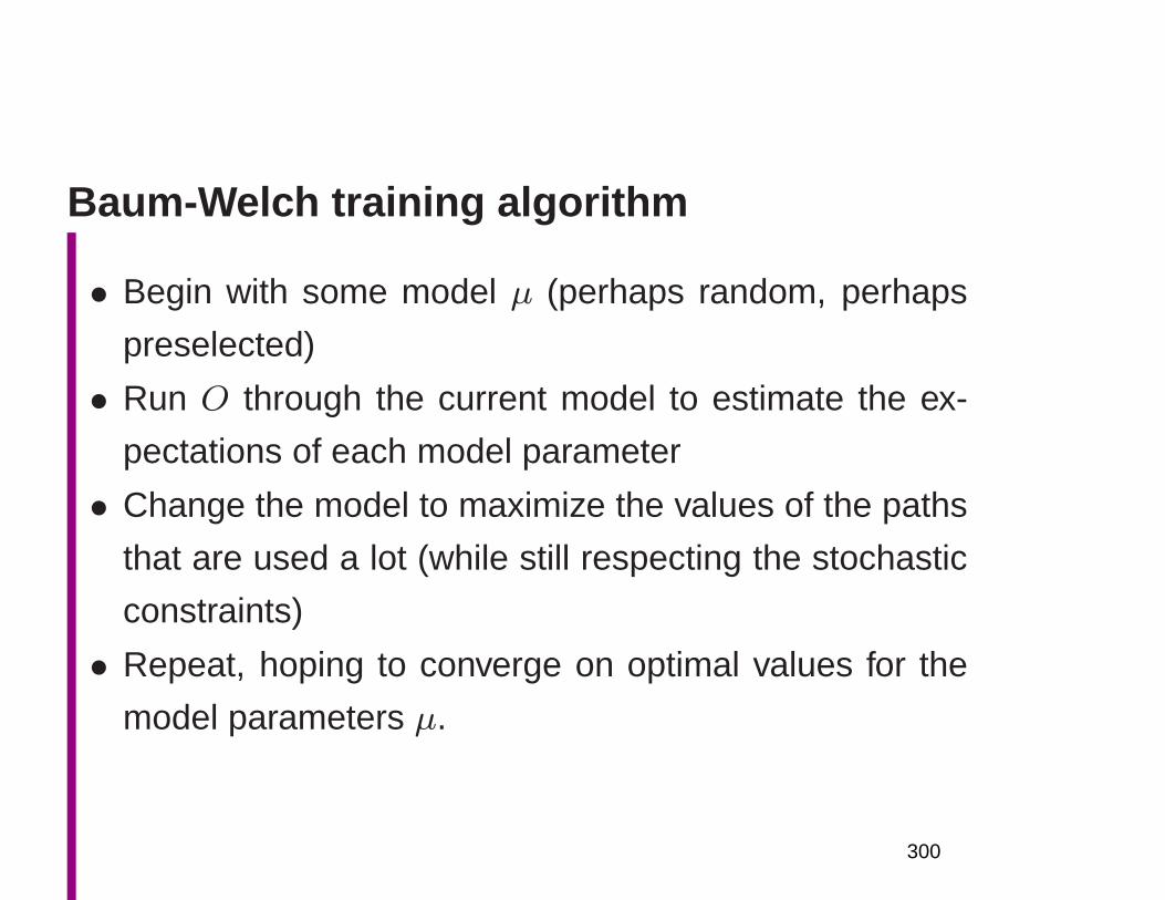
Baum-Welch training algorithm
• Begin with some model µ (perhaps random, perhaps
preselected)
• Run O through the current model to estimate the ex-
pectations of each model parameter
• Change the model to maximize the values of the paths
that are used a lot (while still respecting the stochastic
constraints)
• Repeat, hoping to converge on optimal values for the
model parameters µ.
300
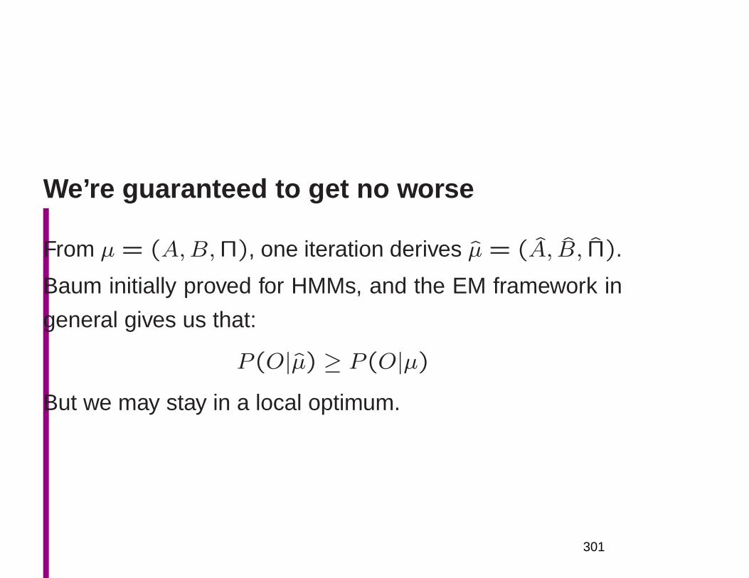
We’re guaranteed to get no worse
From µ = (A,B,Π), one iteration derives µ = (A, B, Π).
Baum initially proved for HMMs, and the EM framework in
general gives us that:
P (O|µ) ≥ P (O|µ)But we may stay in a local optimum.
301
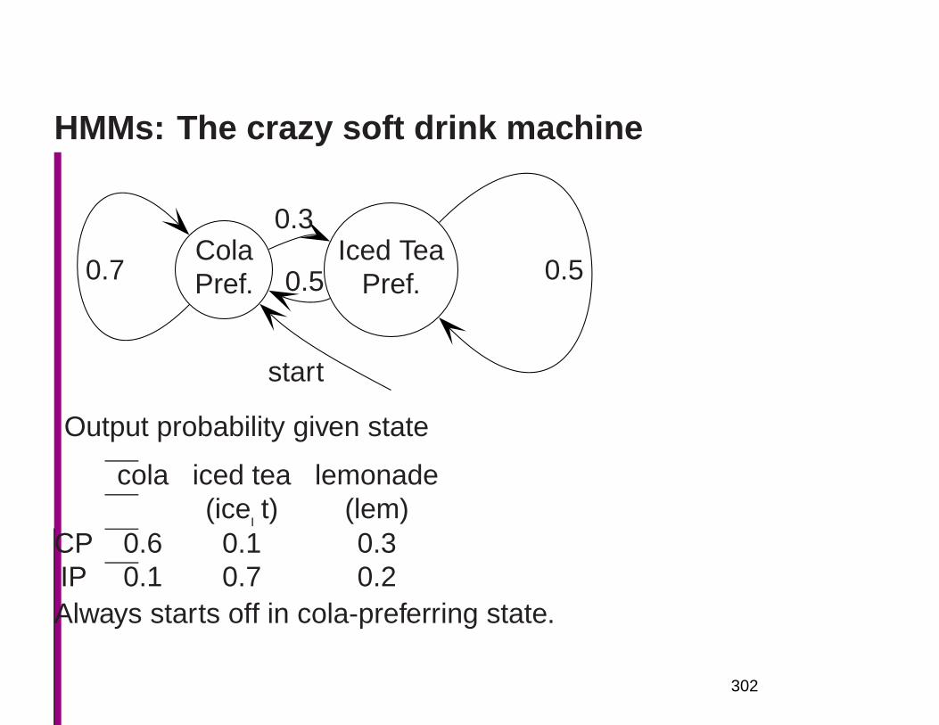
HMMs: The crazy soft drink machine
ColaPref.
Iced TeaPref.
0.3
0.5
start
0.50.7
Output probability given state
cola iced tea lemonade(ice t) (lem)
CP 0.6 0.1 0.3IP 0.1 0.7 0.2Always starts off in cola-preferring state.
302
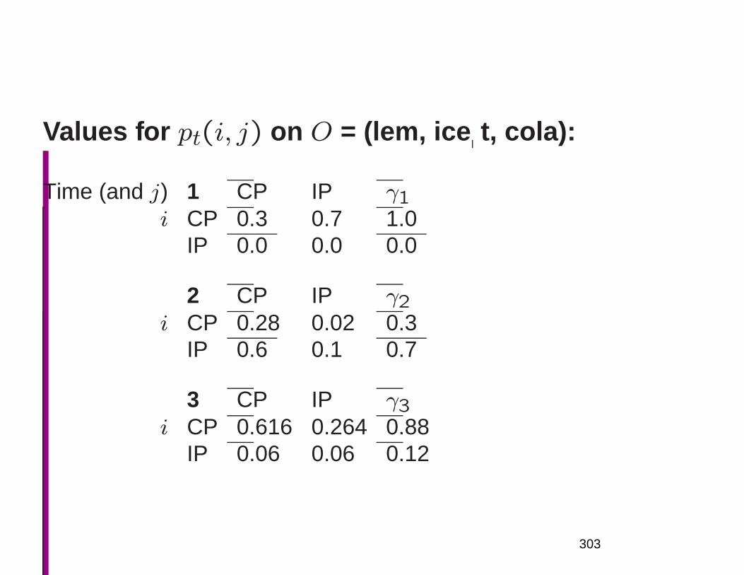
Values for pt(i, j) on O = (lem, ice t, cola):
Time (and j) 1 CP IP γ1i CP 0.3 0.7 1.0
IP 0.0 0.0 0.0
2 CP IP γ2i CP 0.28 0.02 0.3
IP 0.6 0.1 0.7
3 CP IP γ3i CP 0.616 0.264 0.88
IP 0.06 0.06 0.12
303
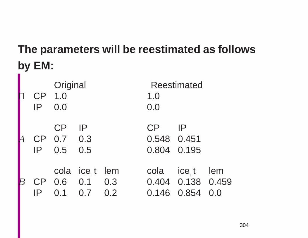
The parameters will be reestimated as followsby EM:
Original ReestimatedΠ CP 1.0 1.0
IP 0.0 0.0
CP IP CP IPA CP 0.7 0.3 0.548 0.451
IP 0.5 0.5 0.804 0.195
cola ice t lem cola ice t lemB CP 0.6 0.1 0.3 0.404 0.138 0.459
IP 0.1 0.7 0.2 0.146 0.854 0.0
304
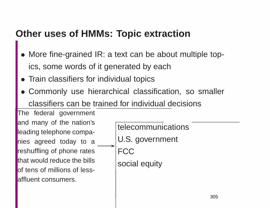
Other uses of HMMs: Topic extraction
• More fine-grained IR: a text can be about multiple top-
ics, some words of it generated by each
• Train classifiers for individual topics
• Commonly use hierarchical classification, so smaller
classifiers can be trained for individual decisionsThe federal governmentand many of the nation’sleading telephone compa-nies agreed today to areshuffling of phone ratesthat would reduce the billsof tens of millions of less-affluent consumers.
telecommunications
U.S. government
FCC
social equity
305
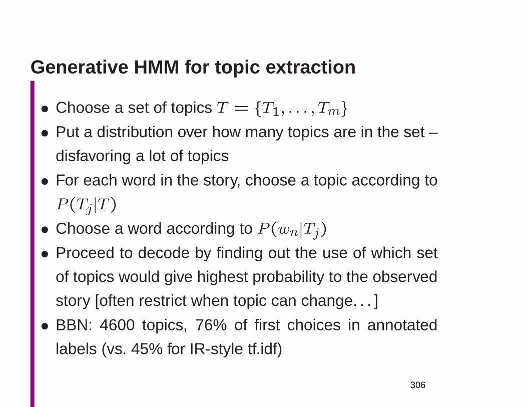
Generative HMM for topic extraction
• Choose a set of topics T = T1, . . . , Tm• Put a distribution over how many topics are in the set –
disfavoring a lot of topics
• For each word in the story, choose a topic according to
P (Tj|T )
• Choose a word according to P (wn|Tj)• Proceed to decode by finding out the use of which set
of topics would give highest probability to the observed
story [often restrict when topic can change. . . ]
• BBN: 4600 topics, 76% of first choices in annotated
labels (vs. 45% for IR-style tf.idf)
306
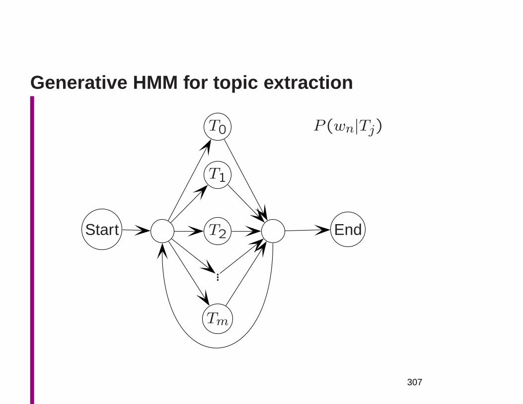
Generative HMM for topic extraction
T0 P (wn|Tj)
T1
Start T2 End
...
Tm
307
Other uses of HMMs: Extracting facts
• The problem with IR: You search for “soldiers attackingrebels” and the top matches are:
– Hutu rebels attacked soldiers in one of Bujumbura’ssuburbs (Google 2000/10/03)
– Sudanese rebels say they have killed or woundedmore than 300 government soldiers (Hotbot 2000/10/03)
– [Altavista: a Confederate soldier’s memorial!]
• We need to be able to match relationships like:
– attack(soldiers, rebels)
• Models that see sentence structure, like HMMs or de-pendency parsers, let us capture these relations, thoughwe still need to deal with synonymy and polysemy
308
Other uses of HMMs: Information Extraction(Freitag and McCallum 1999)
• IE: extracting instance of a relation from text snippets
• States correspond to fields one wishes to extract, token
sequences in the context that are good for identifying
the fields to be extracted, and a background “noise”
state
• Estimation is from tagged data (perhaps supplemented
by EM reestimation over a bigger training set)
• The Viterbi algorithm is used to tag new text
• Things tagged as fields to be extracted are returned
309
Information Extraction (Freitag and McCallum1999)
• State topology is set by hand. Not fully connected
• Use simpler and more complex models, but generally:
– Background state
– Preceding context state(s)
– Target state(s)
– Following context state(s)
• Preceding context states connect only to target state,
etc.
310
Information Extraction (Freitag and McCallum1999)
• Each HMM is for only one field type (e.g., “speaker”)
• Use different HMMs for each field (bad: no real notion
of multi-slot structure)
• Semi-supervised training: target words (generated only
by target states) are marked
• Shrinkage/deleted interpolation is used to generalize
parameter estimates to give more robustness in the
face of data sparseness
• Some other work has done multi-field extraction over
more structured data (Borkar et al. 2001)
311
Information Extraction (Freitag and McCallum1999)
• Tested on seminar announcements and corporate ac-
quisitions data sets
• Performance is generally equal to or better than that of
other information extraction methods
• Though probably more suited to semi-structured text
with clear semantic sorts, than strongly NLP-oriented
problems
• HMMs tend to be especially good for robustness and
high recall
312
Information extraction
• Getting particular fixed semantic relations out of text(e.g., buyer, sell, goods) for DB filling
• Statistical approaches have been explored recently, par-ticularly use of HMMs (Freitag and McCallum 2000)
• States correspond to elements of fields to extract, tokensequences in the context that identify the fields to beextracted, and background “noise” states
• Estimation is from labeled data (perhaps supplementedby EM reestimation over a bigger training set)
• Structure learning used to find a good HMM structure
• The Viterbi algorithm is used to tag new text
• Things tagged as within fields are returned
313
Information extraction: locations and speak-ers
314
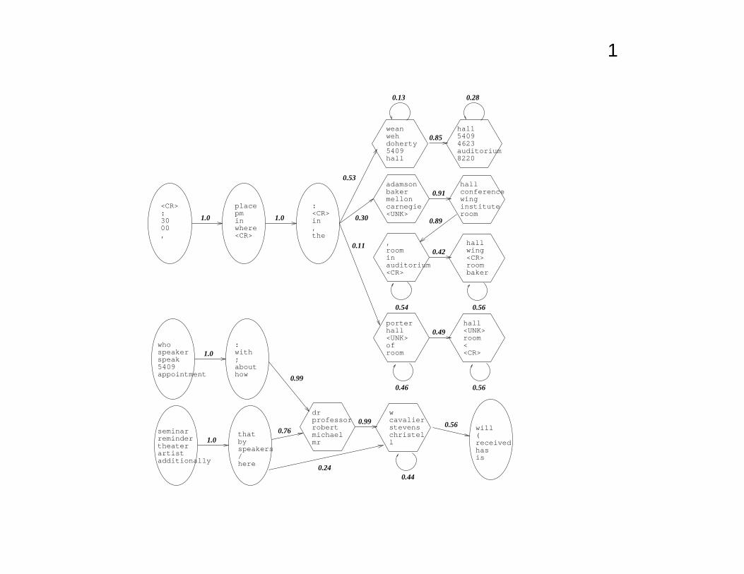
1
,roominauditorium<CR>
hallwing<CR>roombaker
adamsonbakermelloncarnegie<UNK>
hallconferencewinginstituteroom
weanwehdoherty5409hall
hall54094623auditorium8220
1.0 1.0
<CR>:3000,
placepminwhere<CR>
:<CR>in,the
seminarremindertheaterartistadditionally
thatbyspeakers/here
porterhall<UNK>ofroom
hall<UNK>room<<CR>
0.49
0.46 0.56
drprofessorrobertmichaelmr
wcavalierstevenschristell
whospeakerspeak5409appointment
will(receivedhasis
0.53
0.30
0.42
0.91
0.11
0.89
0.85
0.54 0.56
0.13 0.28
1.0
1.0
0.99
0.76
0.24
0.99
0.44
0.56
:with;abouthow
HMMs in Computational Biology
• Determining coding/non-coding regions of DNA
• Determining protein-binding sites of DNA
• Aligning and analyzing protein families
• Aligning DNA regions
• Unlike human languages, observation alphabets are
normally small, and so clever smoothing/shrinkage meth-
ods are less necessary
315
Identifying G-protein-coupled receptors (Baldiand Chauvin 1994)
• Long but very variable length chains (200–1200) of amino
acids
• HMM trained on known examples, with states equal to
average length
• Effectively HMM is computing a kind of probabilistic
‘edit distance’, measuring changes, repeats, and dele-
tions
• Model can effectively discriminate GPCR sequences
from random or non-GPCR sequences based on cal-
culated log-likelihood of sequence
316
Gene finding in DNA sequences (Krogh, Mianand Haussler 1994)
• Finds protein-coding genes in E. coli DNA.
• HMM states model codons, intergenic regions (incl. palin-
dromic sequences, etc.)
• Allows for insertions and deletions
• HMM parameters estimated from 1 million nucleotides
of annotated DNA
• On independent data, model finds exact location of about
80% of known E. coli genes, and approximate location
of a further 10%.
• It also potentially finds several new genes. . . .
317
Summary
• HMMs are one simple, well-understood, and generally
effective form of probabilistic model
• Their math is well understood
• Suitable for problems with a linear (or finite-state or
time-series) character
• Widely used in speech, language, vision & movement,
and DNA alignment applications
• Probabilistic context-free grammar and richer models
also exist when richer recursive structure is required.
318

Extra variant slides
319
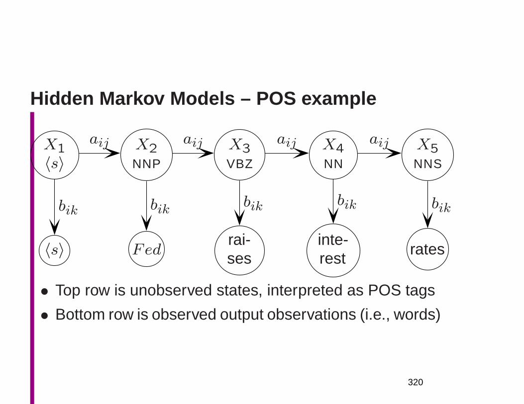
Hidden Markov Models – POS example
X1〈s〉
X2NNP
X3VBZ
X4NN
X5NNS
〈s〉 Fedrai-ses
inte-rest
rates
aij aij aij aij
bik bik bik bik bik
• Top row is unobserved states, interpreted as POS tags
• Bottom row is observed output observations (i.e., words)
320
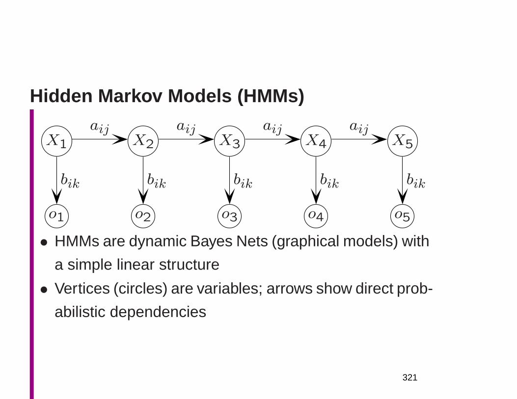
Hidden Markov Models (HMMs)
X1 X2 X3 X4 X5
o1 o2 o3 o4 o5
aij aij aij aij
bik bik bik bik bik
• HMMs are dynamic Bayes Nets (graphical models) with
a simple linear structure
• Vertices (circles) are variables; arrows show direct prob-
abilistic dependencies
321
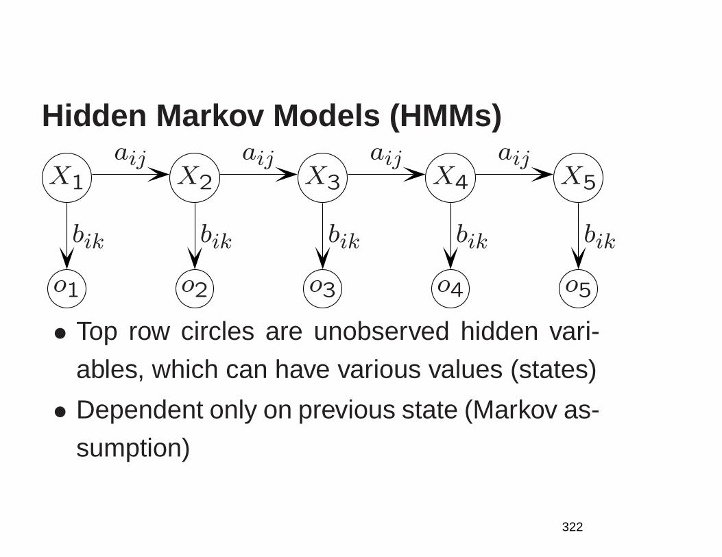
Hidden Markov Models (HMMs)
X1 X2 X3 X4 X5
o1 o2 o3 o4 o5
aij aij aij aij
bik bik bik bik bik
• Top row circles are unobserved hidden vari-
ables, which can have various values (states)
• Dependent only on previous state (Markov as-
sumption)
322
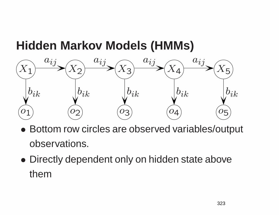
Hidden Markov Models (HMMs)
X1 X2 X3 X4 X5
o1 o2 o3 o4 o5
aij aij aij aij
bik bik bik bik bik
• Bottom row circles are observed variables/output
observations.
• Directly dependent only on hidden state above
them
323
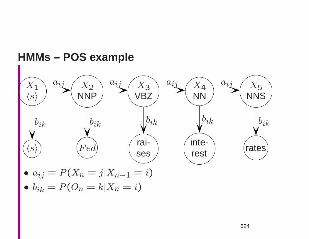
HMMs – POS example
X1〈s〉
X2NNP
X3VBZ
X4NN
X5NNS
〈s〉 Fedrai-ses
inte-rest
rates
aij aij aij aij
bik bik bik bik bik
• aij = P (Xn = j|Xn−1 = i)
• bik = P (On = k|Xn = i)
324
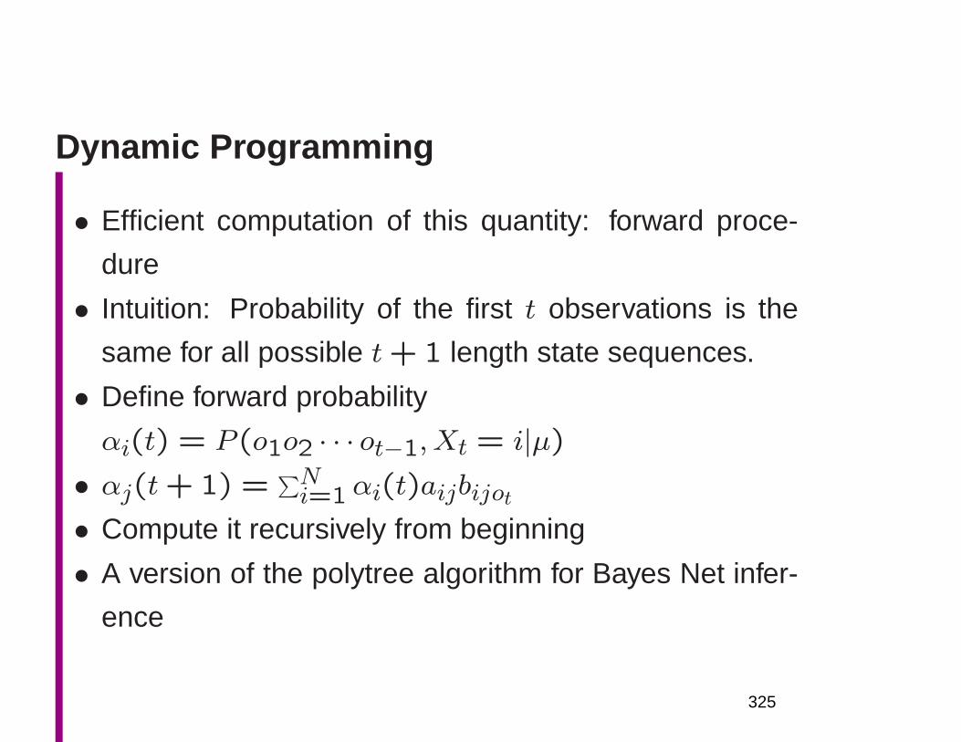
Dynamic Programming
• Efficient computation of this quantity: forward proce-
dure
• Intuition: Probability of the first t observations is the
same for all possible t+ 1 length state sequences.
• Define forward probability
αi(t) = P (o1o2 · · · ot−1, Xt = i|µ)• αj(t+ 1) =
∑Ni=1αi(t)aijbijot
• Compute it recursively from beginning
• A version of the polytree algorithm for Bayes Net infer-
ence
325
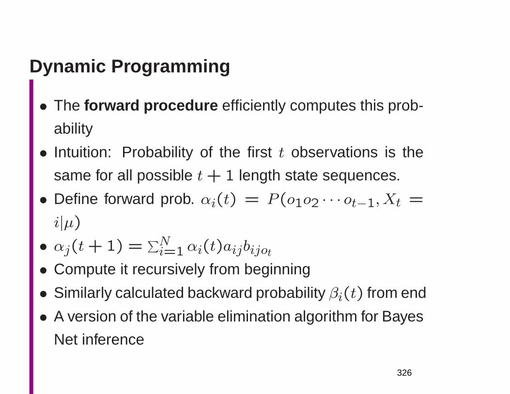
Dynamic Programming
• The forward procedure efficiently computes this prob-
ability
• Intuition: Probability of the first t observations is the
same for all possible t+ 1 length state sequences.
• Define forward prob. αi(t) = P (o1o2 · · · ot−1, Xt =
i|µ)• αj(t+ 1) =
∑Ni=1αi(t)aijbijot
• Compute it recursively from beginning
• Similarly calculated backward probability βi(t) from end
• A version of the variable elimination algorithm for Bayes
Net inference
326
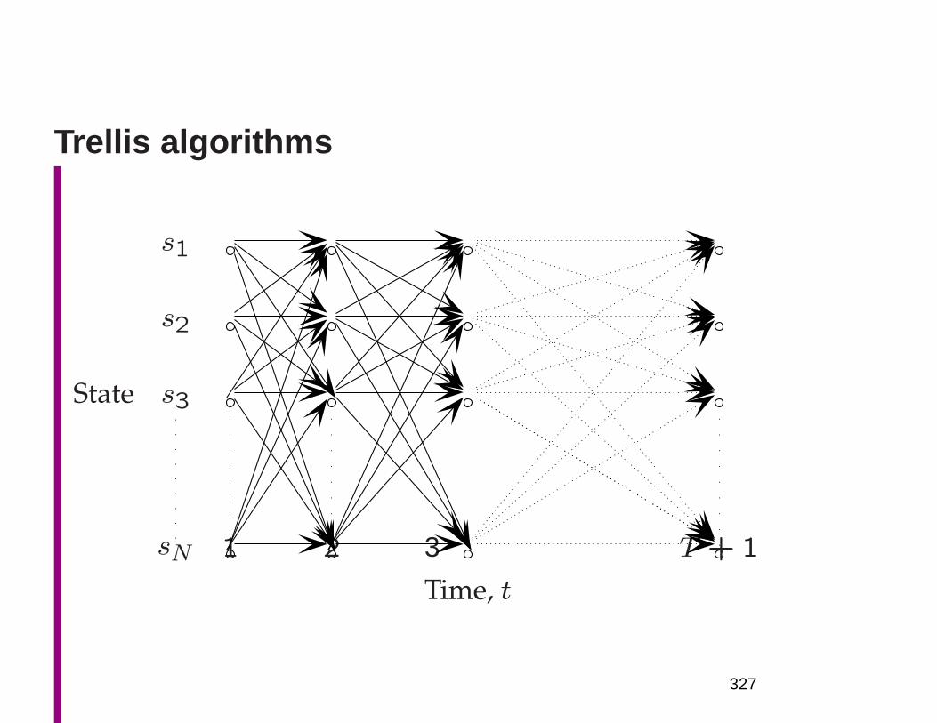
Trellis algorithms
s1
s2
State s3
sN 1 2 3
Time, t
T + 1
327
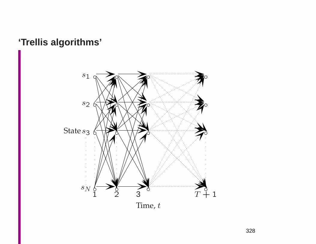
‘Trellis algorithms’
s1
s2
States3
sN1 2 3
Time, t
T + 1
328
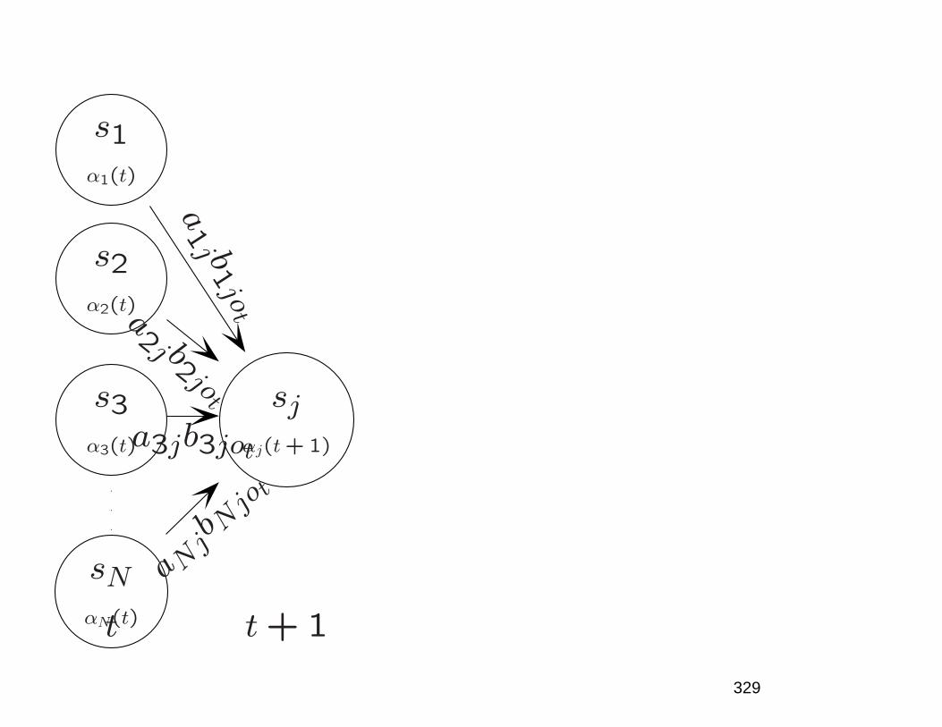
s1α1(t)
s2α2(t)
s3α3(t)
sjαj(t+ 1)
sNαN(t)t t+ 1
a1j b
1jota
2j b2jo
t
a3jb3jot
a Njb Njot
329
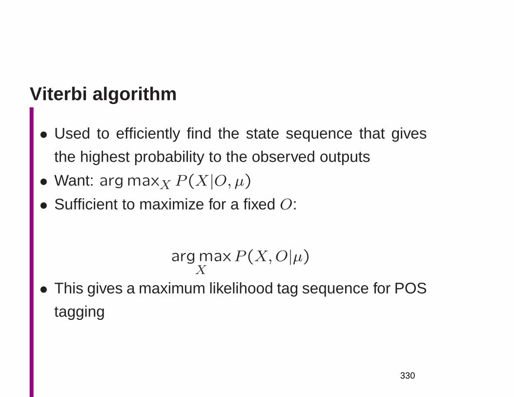
Viterbi algorithm
• Used to efficiently find the state sequence that gives
the highest probability to the observed outputs
• Want: argmaxX P (X|O, µ)• Sufficient to maximize for a fixed O:
argmaxX
P (X,O|µ)
• This gives a maximum likelihood tag sequence for POS
tagging
330
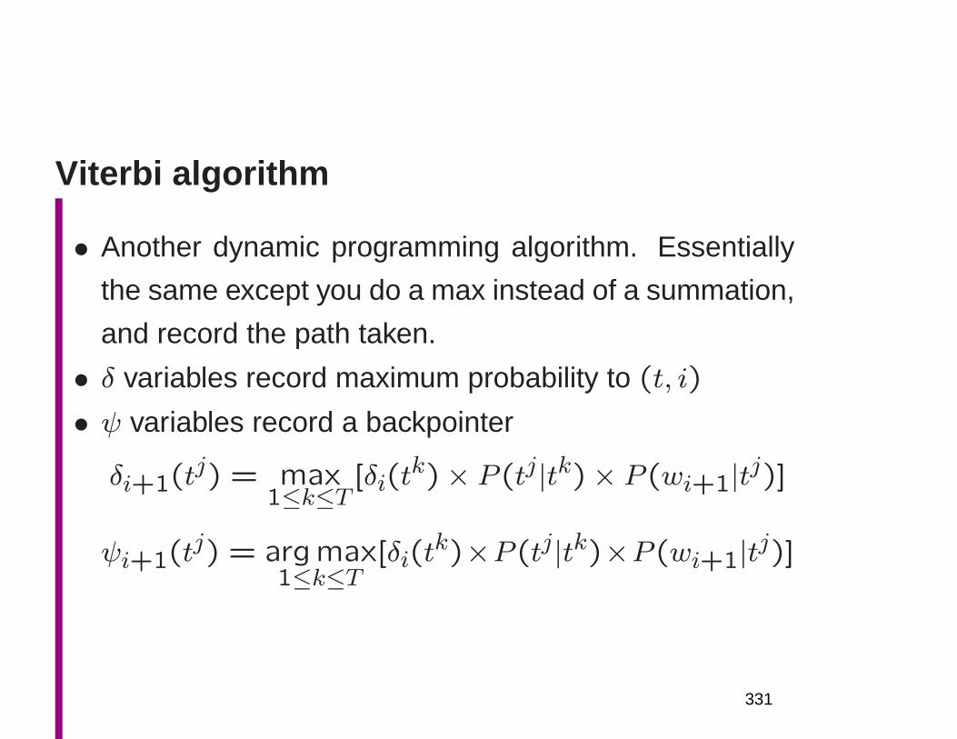
Viterbi algorithm
• Another dynamic programming algorithm. Essentially
the same except you do a max instead of a summation,
and record the path taken.
• δ variables record maximum probability to (t, i)
• ψ variables record a backpointer
δi+1(tj) = max
1≤k≤T[δi(t
k)× P (tj|tk)× P (wi+1|tj)]
ψi+1(tj) = argmax
1≤k≤T[δi(t
k)×P (tj|tk)×P (wi+1|tj)]
331
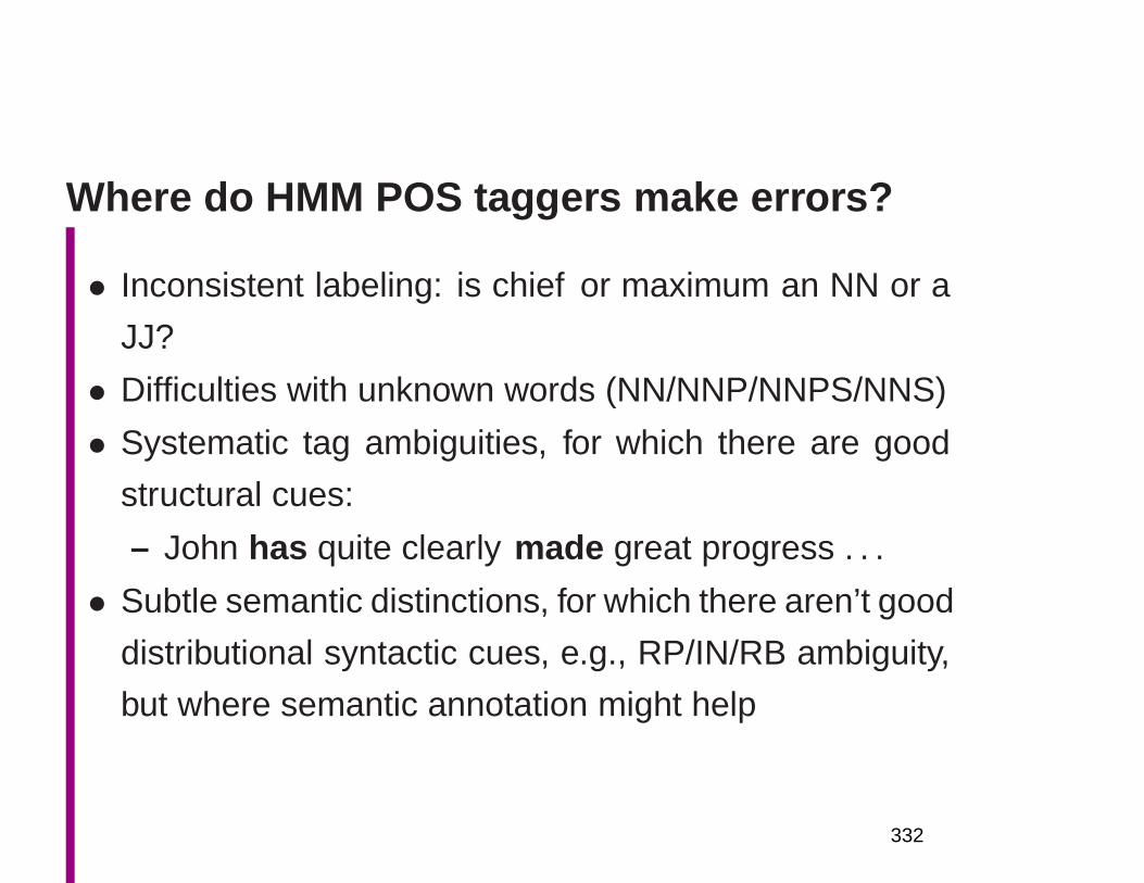
Where do HMM POS taggers make errors?
• Inconsistent labeling: is chief or maximum an NN or a
JJ?
• Difficulties with unknown words (NN/NNP/NNPS/NNS)
• Systematic tag ambiguities, for which there are good
structural cues:
– John has quite clearly made great progress . . .
• Subtle semantic distinctions, for which there aren’t good
distributional syntactic cues, e.g., RP/IN/RB ambiguity,
but where semantic annotation might help
332
Probabilistic |StochasticContext-Free Grammars
(PCFGs)
FSNLP, chapter 11
Christopher Manning andHinrich Schütze
© 1999–2002333
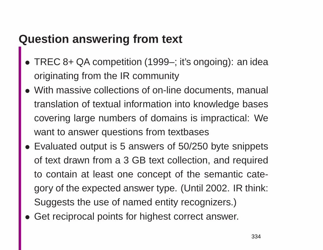
Question answering from text
• TREC 8+ QA competition (1999–; it’s ongoing): an ideaoriginating from the IR community
• With massive collections of on-line documents, manualtranslation of textual information into knowledge basescovering large numbers of domains is impractical: Wewant to answer questions from textbases
• Evaluated output is 5 answers of 50/250 byte snippetsof text drawn from a 3 GB text collection, and requiredto contain at least one concept of the semantic cate-gory of the expected answer type. (Until 2002. IR think:Suggests the use of named entity recognizers.)
• Get reciprocal points for highest correct answer.
334
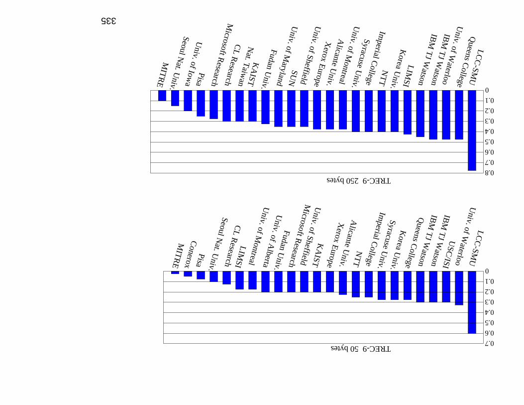
IBM
TJ W
atsonIB
M T
J Watson
LCC
-SM
UU
niv. of Waterloo
Queens C
ollegeK
orea Univ.
Syracuse U
niv.Im
perial CollegeN
TT
Alicante U
niv.X
erox Europe
KA
IST
Univ. of S
heffieldM
icrosoft Research
Fudan U
niv.U
niv. of Alberta
Univ. of M
ontrealLIM
SI
CL R
esearchS
eoul Nat. U
niv.P
isaC
oneroxM
ITR
E
0.7
0.6
0.5
0.4
0.3
0.2
0.1
TREC-9 50 bytes
IBM
TJ W
atsonIB
M T
J Watson
LCC
-SM
U
Korea U
niv.
Pisa
0.7
0.6
0.5
0.4
0.3
0.2
0.1
0.8
Queens C
ollegeU
niv. of Waterloo
LIMS
I
NT
TIm
perial College
Syracuse U
niv.U
niv. of Montreal
Alicante U
niv.X
erox Europe
Univ. of S
heffieldS
UN
Univ. of M
arylandF
udan Univ.
KA
IST
Nat. T
aiwan
CL R
esearchM
icrosoft Research
Univ. of Iow
a
MIT
RE
Seoul N
at. Univ.
0
0
US
C/IS
I
TREC-9 250 bytes
335
Pasca and Harabagiu (2001) demonstrates thevalue of sophisticated NLP processing
• Good IR is needed: paragraph retrieval based on SMART
• Large taxonomy of question types and expected an-swer types is crucial
• Parsing: A statistical parser (modeled on Collins 1997)is used to parse questions, relevant text for answers,and WordNet to build a knowledge base for reasoning
• Controlled query expansion loops (morphological, lexi-cal synonyms, and semantic relations) are all importantin retrieving the correct answer.
• Answer ranking by ML method based on this informa-tion surpasses IR-style empirical methods.
336

Question Answering Example (1)
• Q261: What company sells most greetings cards ?
• sells(ORGANIZATION, cards(greeting), most)
• “Hallmark remains the largest maker of greeting cards”maker(ORGANIZATION(Hallmark), cards(greeting), largest)
• Need an entailment between producing, or making andselling goods
• Derived from WordNet, since synset make, produce,create has the genus manufacture , defined in the gloss
of its nominalization as (for ) sale
• Also, need most ≈ largest
• Therefore the semantic form of question Q261 and its
illustrated answer are similar
337
Question Answering Example (2)
• How hot does the inside of an active volcano get ?
• get(TEMPERATURE, inside(volcano(active)))
• “lava fragments belched out of the mountain were ashot as 300 degrees Fahrenheit”
• fragments(lava, TEMPERATURE(degrees(300)),belched(out, mountain))
• – volcano ISA mountain– lava ISPARTOF volcano lava inside volcano– fragments of lava HAVEPROPERTIESOF lava
• The needed semantic information is available in Word-Net definitions, and was successfully translated into aform that can be used for rough ‘proofs’
338
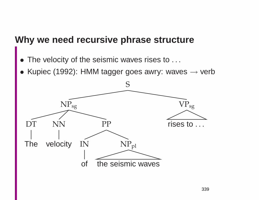
Why we need recursive phrase structure
• The velocity of the seismic waves rises to . . .
• Kupiec (1992): HMM tagger goes awry: waves→ verb
S
NPsg
DT
The
NN
velocity
PP
IN
of
NPpl
the seismic waves
VPsg
rises to . . .
339
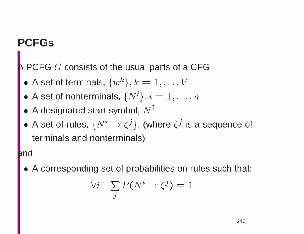
PCFGs
A PCFG G consists of the usual parts of a CFG
• A set of terminals, wk, k = 1, . . . , V
• A set of nonterminals, N i, i = 1, . . . , n
• A designated start symbol, N1
• A set of rules, N i → ζj, (where ζj is a sequence of
terminals and nonterminals)
and
• A corresponding set of probabilities on rules such that:
∀i ∑
jP (N i→ ζj) = 1
340
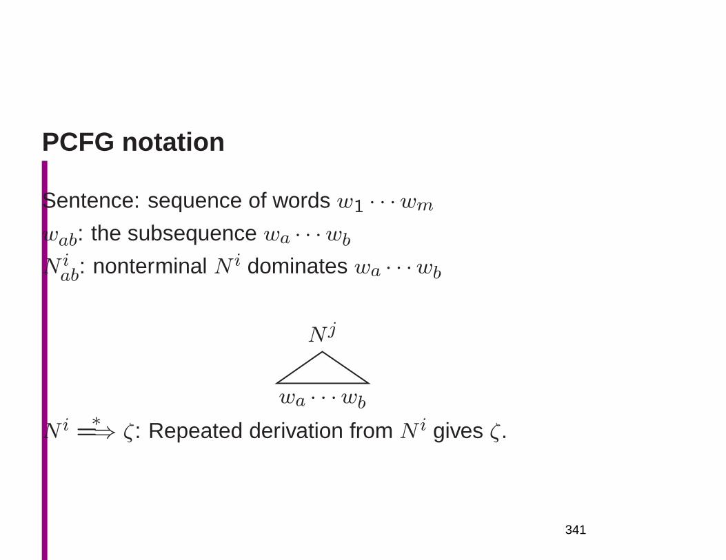
PCFG notation
Sentence: sequence of words w1 · · ·wmwab: the subsequence wa · · ·wbN iab: nonterminal N i dominates wa · · ·wb
Nj
wa · · ·wbN i ∗
=⇒ ζ: Repeated derivation from N i gives ζ.
341
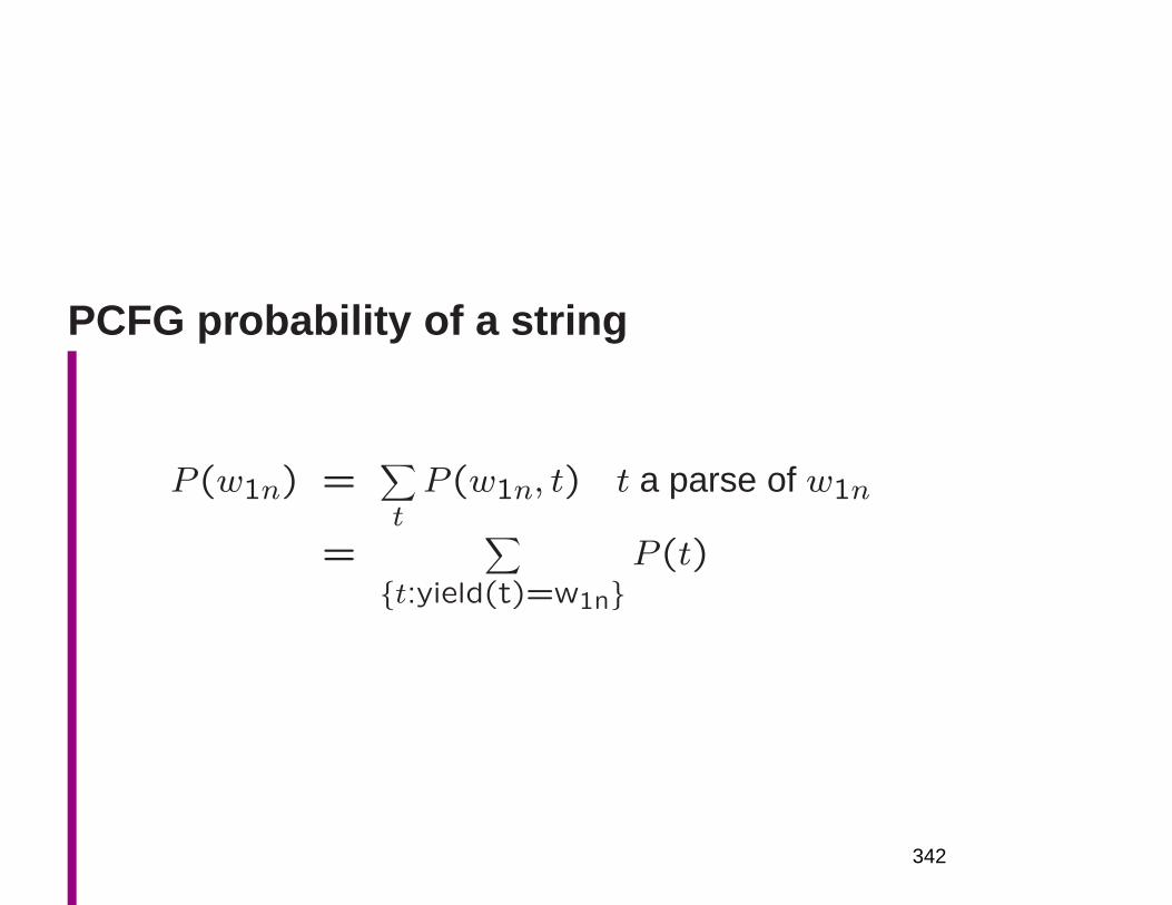
PCFG probability of a string
P (w1n) =∑
tP (w1n, t) t a parse of w1n
=∑
t:yield(t)=w1nP (t)
342
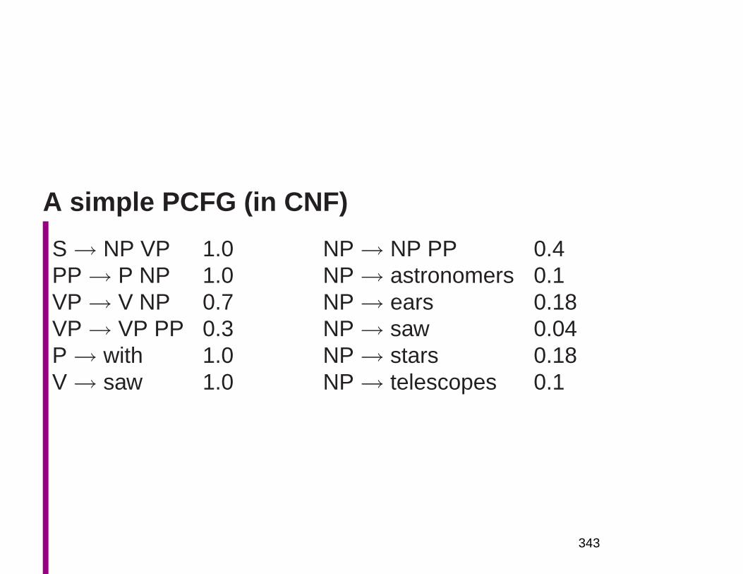
A simple PCFG (in CNF)
S→ NP VP 1.0 NP→ NP PP 0.4PP→ P NP 1.0 NP→ astronomers 0.1VP→ V NP 0.7 NP→ ears 0.18VP→ VP PP 0.3 NP→ saw 0.04P→ with 1.0 NP→ stars 0.18V→ saw 1.0 NP→ telescopes 0.1
343
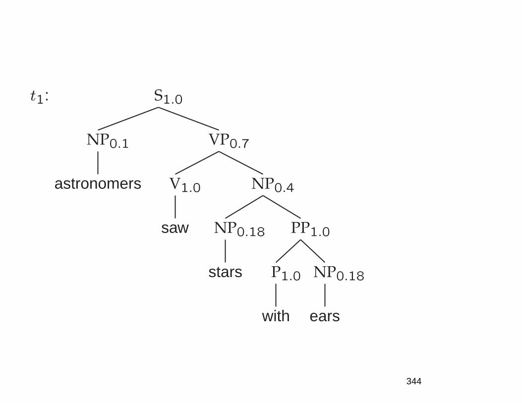
t1: S1.0
NP0.1
astronomers
VP0.7
V1.0
saw
NP0.4
NP0.18
stars
PP1.0
P1.0
with
NP0.18
ears
344
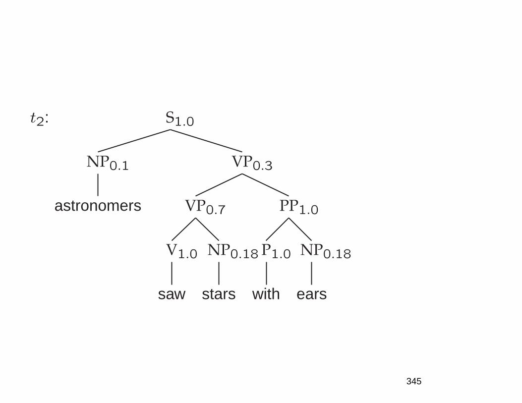
t2: S1.0
NP0.1
astronomers
VP0.3
VP0.7
V1.0
saw
NP0.18
stars
PP1.0
P1.0
with
NP0.18
ears
345
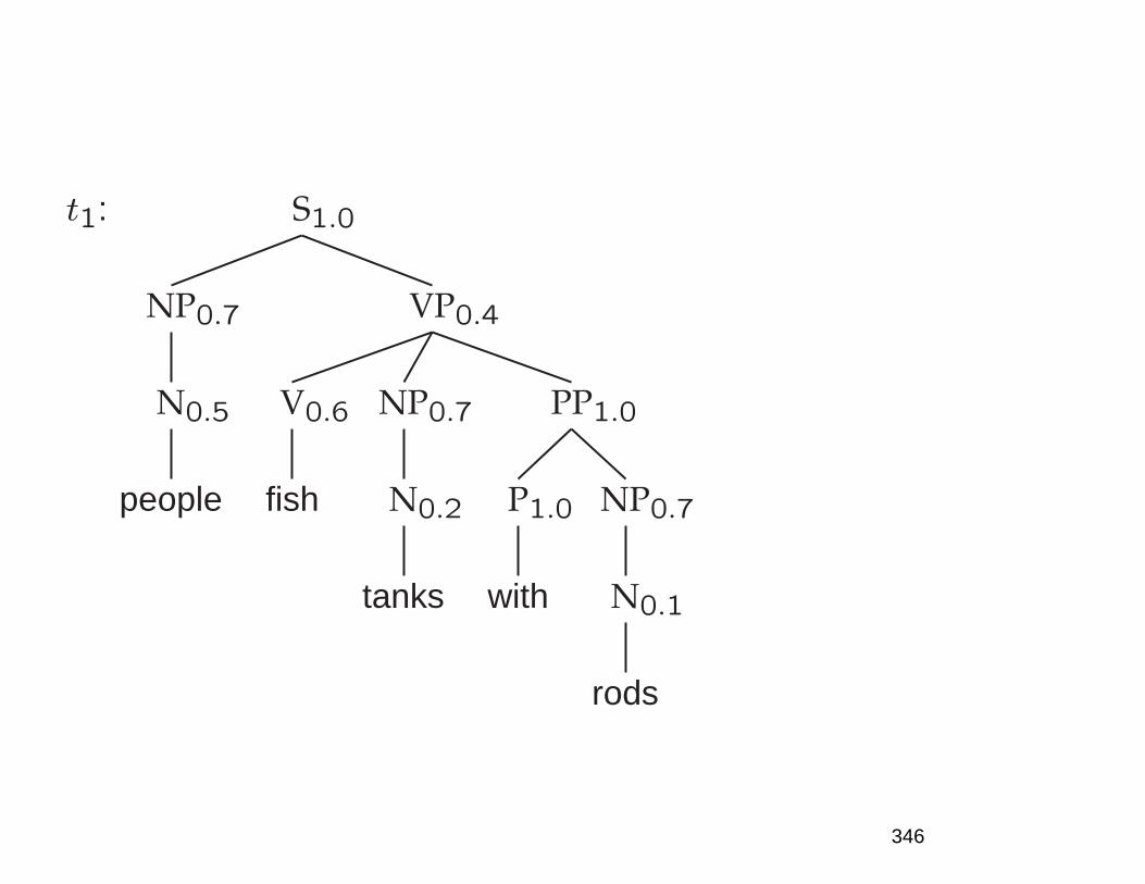
t1: S1.0
NP0.7
N0.5
people
VP0.4
V0.6
fish
NP0.7
N0.2
tanks
PP1.0
P1.0
with
NP0.7
N0.1
rods
346
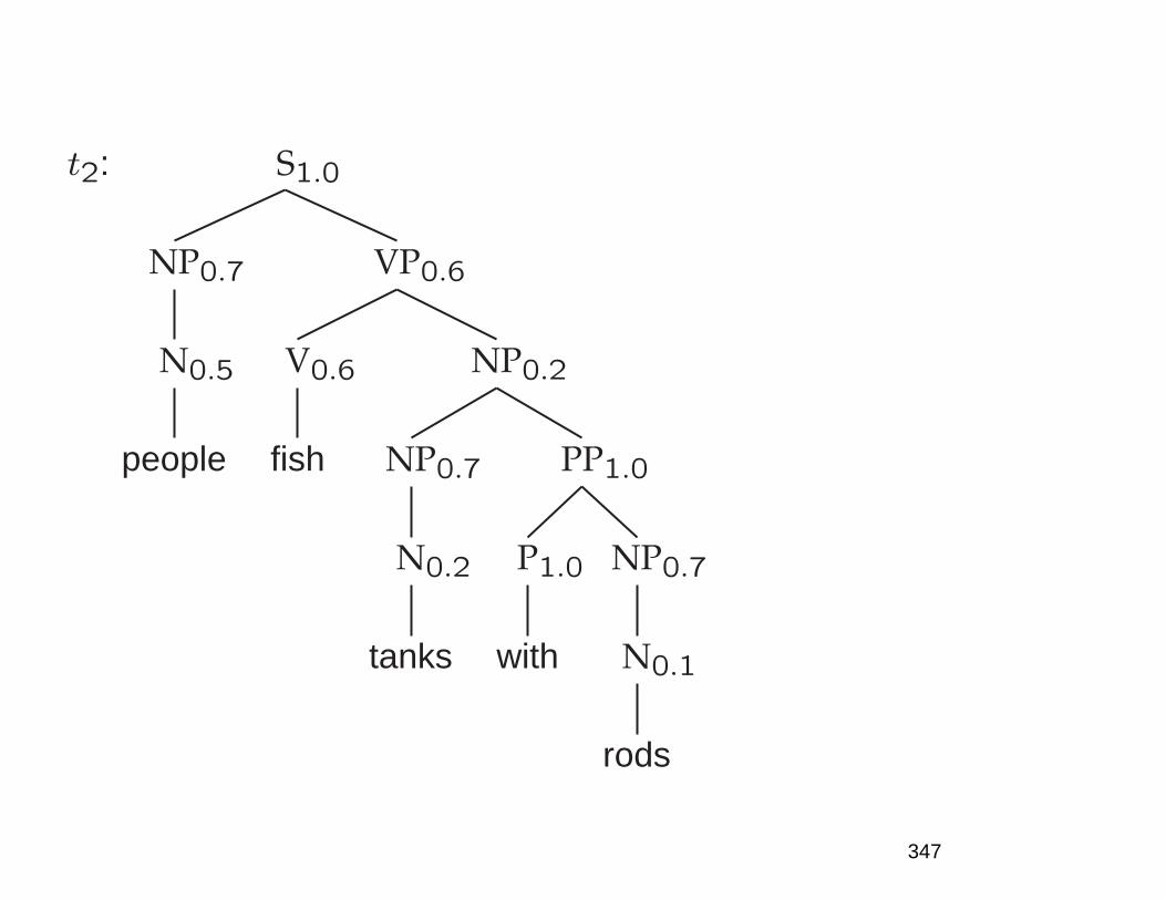
t2: S1.0
NP0.7
N0.5
people
VP0.6
V0.6
fish
NP0.2
NP0.7
N0.2
tanks
PP1.0
P1.0
with
NP0.7
N0.1
rods
347
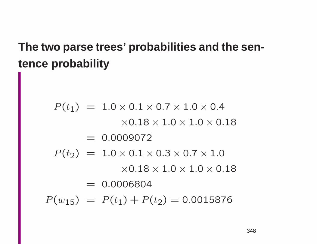
The two parse trees’ probabilities and the sen-tence probability
P (t1) = 1.0× 0.1× 0.7× 1.0× 0.4
×0.18× 1.0× 1.0× 0.18
= 0.0009072
P (t2) = 1.0× 0.1× 0.3× 0.7× 1.0
×0.18× 1.0× 1.0× 0.18
= 0.0006804
P (w15) = P (t1) + P (t2) = 0.0015876
348
Attachment ambiguities: A key parsing deci-sion
• The main problem in parsing is working out how to
‘attach’ various kinds of constituents – PPs, adverbial
or participial phrases, coordinations, and so on
• Prepositional phrase attachment
– I saw the man with a telescope
• What does with a telescope modify?
– The verb saw?
– The noun man?
• Is the problem ‘AI-complete’? Yes, but . . .
349
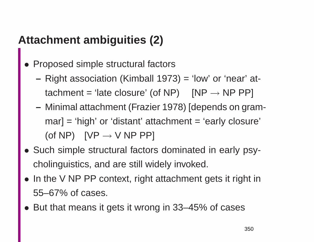
Attachment ambiguities (2)
• Proposed simple structural factors
– Right association (Kimball 1973) = ‘low’ or ‘near’ at-
tachment = ‘late closure’ (of NP) [NP→ NP PP]
– Minimal attachment (Frazier 1978) [depends on gram-
mar] = ‘high’ or ‘distant’ attachment = ‘early closure’
(of NP) [VP→ V NP PP]
• Such simple structural factors dominated in early psy-
cholinguistics, and are still widely invoked.
• In the V NP PP context, right attachment gets it right in
55–67% of cases.
• But that means it gets it wrong in 33–45% of cases
350

Importance of lexical factors
• Words are good predictors (or even inducers) of attach-
ment (even absent understanding):
– The children ate the cake with a spoon.
– The children ate the cake with frosting.
– Moscow sent more than 100,000 soldiers into Afghanistan
– Sydney Water breached an agreement with NSW
Health
• Ford et al. (1982):
– Ordering is jointly determined by strengths of al-
ternative lexical forms, alternative syntactic rewrite
rules, and the sequence of hypotheses in parsing
351
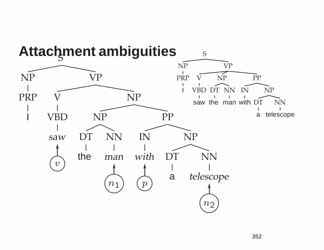
Attachment ambiguities S
NP
PRP
I
VP
V
VBD
saw
NP
DT
the
NN
man
PP
IN
with
NP
DT
a
NN
telescope
S
NP
PRP
I
VP
V
VBD
saw
v
NP
NP
DT
the
NN
man
n1
PP
IN
with
p
NP
DT
a
NN
telescope
n2
352
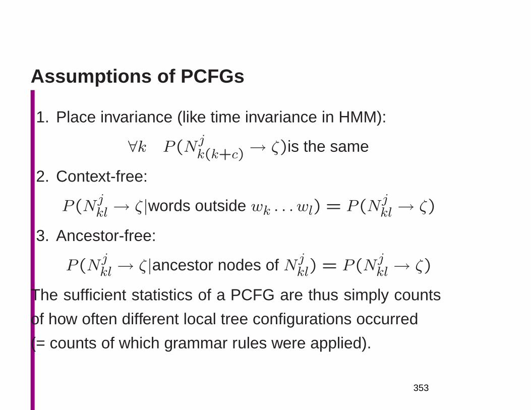
Assumptions of PCFGs
1. Place invariance (like time invariance in HMM):
∀k P (Njk(k+c) → ζ)is the same
2. Context-free:
P (Njkl → ζ|words outside wk . . . wl) = P (N
jkl → ζ)
3. Ancestor-free:
P (Njkl → ζ|ancestor nodes of Nj
kl) = P (Njkl → ζ)
The sufficient statistics of a PCFG are thus simply counts
of how often different local tree configurations occurred
(= counts of which grammar rules were applied).
353
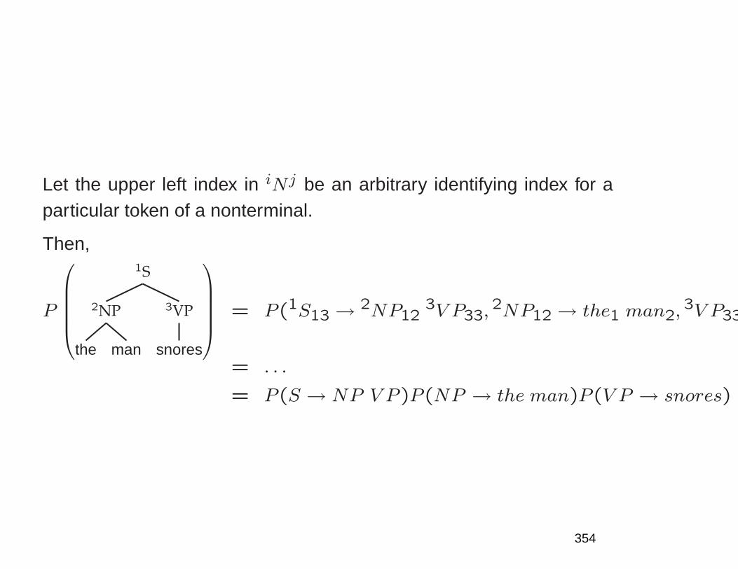
Let the upper left index in iNj be an arbitrary identifying index for aparticular token of a nonterminal.
Then,
P
1S
2NP
the man
3VP
snores
= P(1S13 → 2NP123V P33,
2NP12 → the1 man2,3V P33
= . . .
= P(S → NP V P)P(NP → the man)P(V P → snores)
354

Some features of PCFGs
Reasons to use a PCFG, and some idea of their limitations:
• Partial solution for grammar ambiguity: a PCFG givessome idea of the plausibility of a sentence.• But, in the simple case, not a very good idea, as in-
dependence assumptions are two strong (e.g., not lex-icalized).
• Gives a probabilistic language model for English.• In the simple case, a PCFG is a worse language model
for English than a trigram model.• Better for grammar induction (Gold 1967 vs. Horning
1969)
• Robustness. (Admit everything with low probability.)
355
Some features of PCFGs
• A PCFG encodes certain biases, e.g., that smaller trees
are normally more probable.
• One can hope to combine the strengths of a PCFG and
a trigram model.
We’ll look at simple PCFGs first. They have certain in-
adequacies, but we’ll see that most of the state-of-the-art
probabilistic parsers are fundamentally PCFG models, just
with various enrichments to the grammar
356
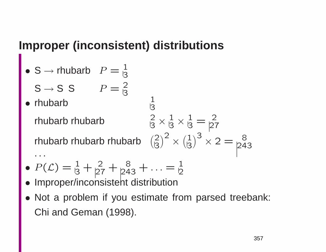
Improper (inconsistent) distributions
• S→ rhubarb P = 13
S→ S S P = 23
• rhubarb 13
rhubarb rhubarb 23 ×
13 ×
13 = 2
27
rhubarb rhubarb rhubarb(
23
)2 ×(
13
)3 × 2 = 8243
. . .• P (L) = 1
3 + 227 + 8
243 + . . . = 12
• Improper/inconsistent distribution
• Not a problem if you estimate from parsed treebank:
Chi and Geman (1998).
357
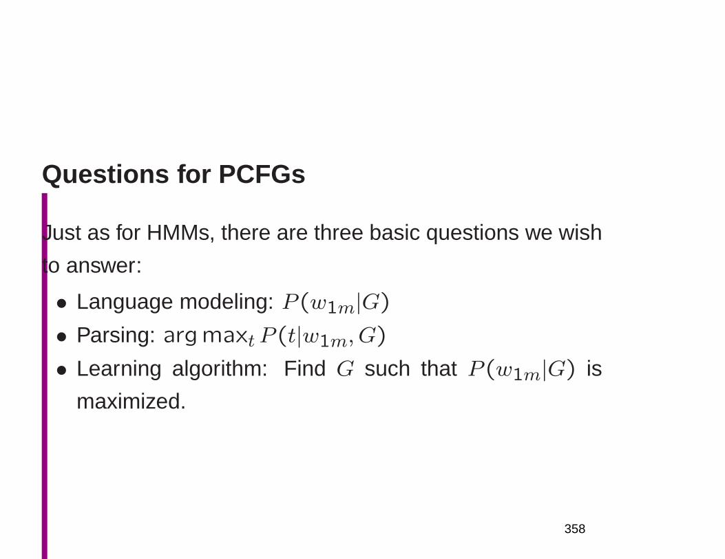
Questions for PCFGs
Just as for HMMs, there are three basic questions we wish
to answer:
• Language modeling: P (w1m|G)
• Parsing: argmaxtP (t|w1m, G)
• Learning algorithm: Find G such that P (w1m|G) is
maximized.
358
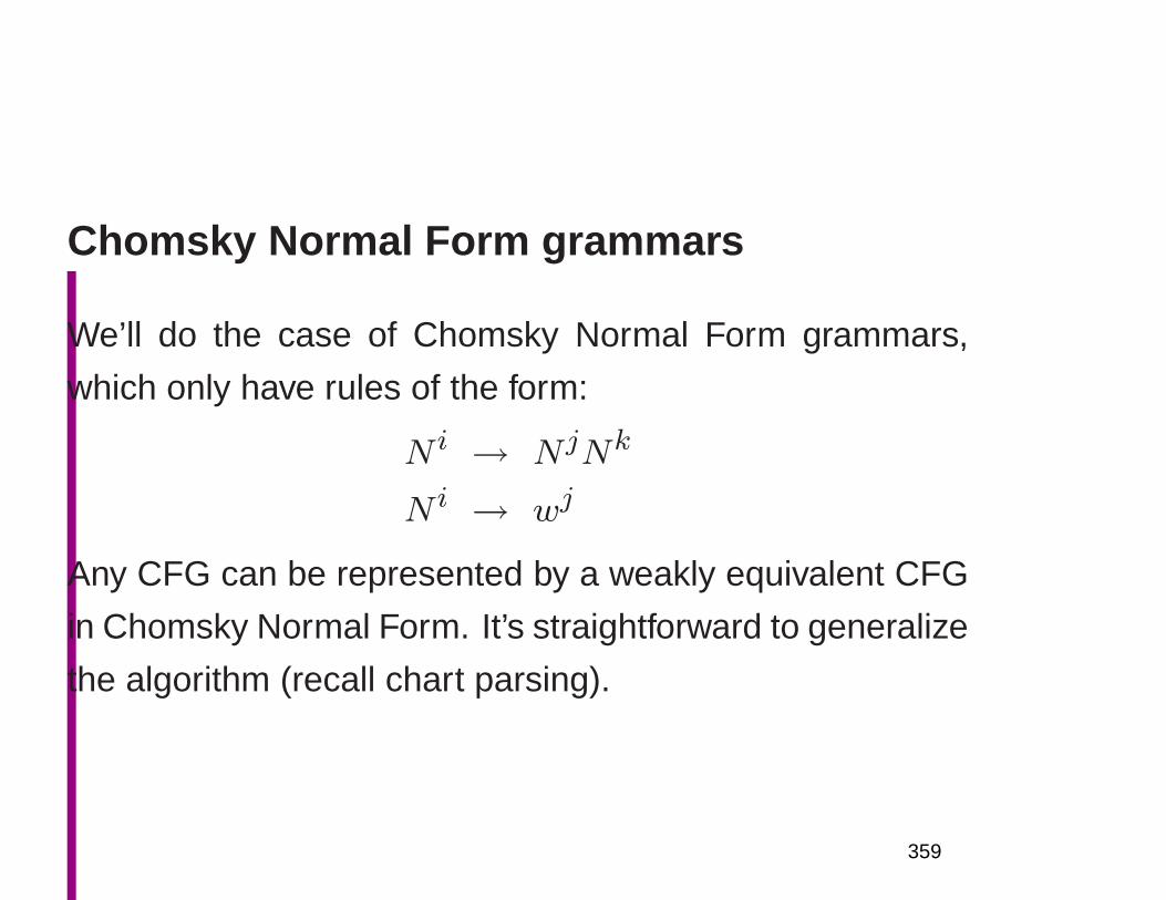
Chomsky Normal Form grammars
We’ll do the case of Chomsky Normal Form grammars,
which only have rules of the form:
N i → NjNk
N i → wj
Any CFG can be represented by a weakly equivalent CFG
in Chomsky Normal Form. It’s straightforward to generalize
the algorithm (recall chart parsing).
359
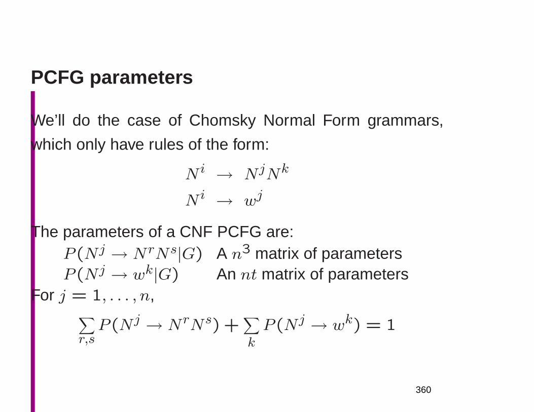
PCFG parameters
We’ll do the case of Chomsky Normal Form grammars,
which only have rules of the form:
N i → NjNk
N i → wj
The parameters of a CNF PCFG are:P (Nj → NrNs|G) A n3 matrix of parametersP (Nj → wk|G) An nt matrix of parameters
For j = 1, . . . , n,∑
r,sP (Nj → NrNs) +
∑
kP (Nj → wk) = 1
360
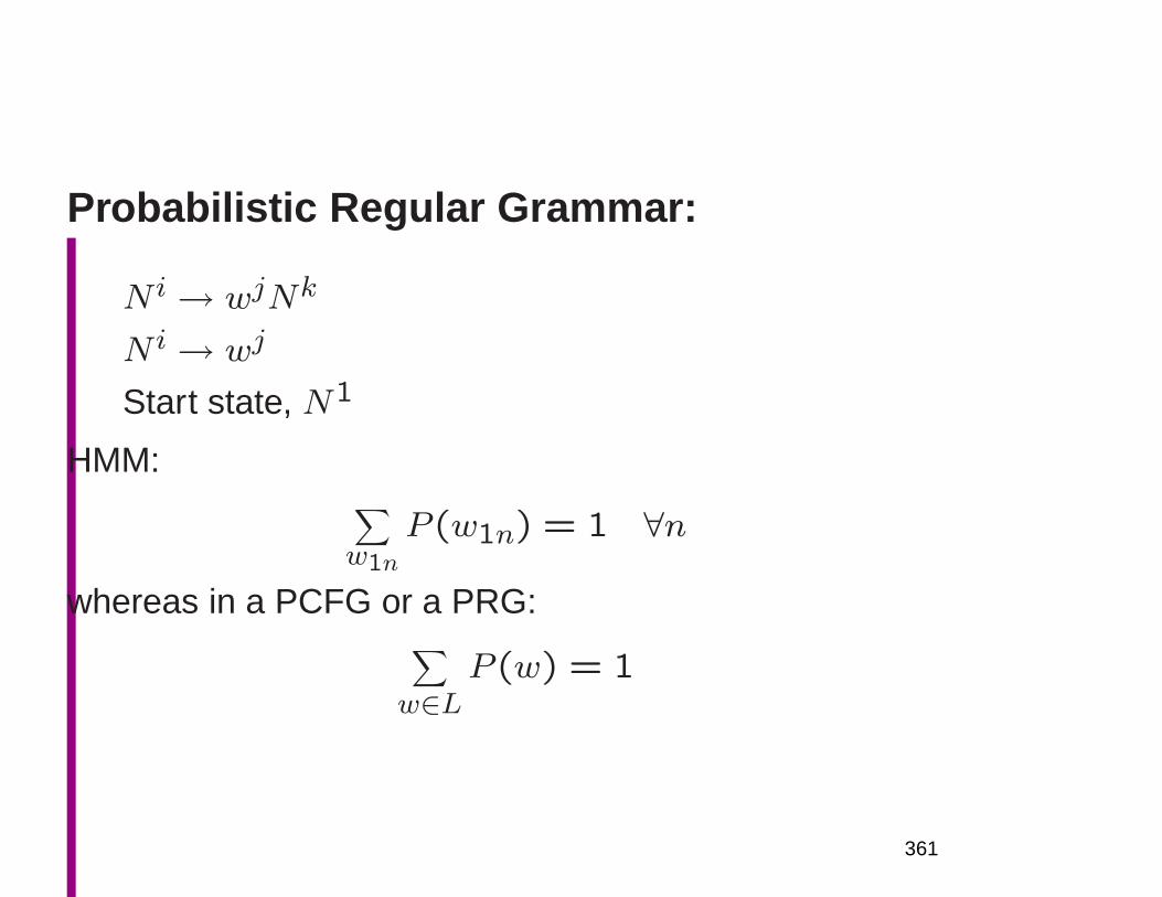
Probabilistic Regular Grammar:
N i→ wjNk
N i→ wj
Start state, N1
HMM:∑
w1n
P (w1n) = 1 ∀n
whereas in a PCFG or a PRG:∑
w∈LP (w) = 1
361
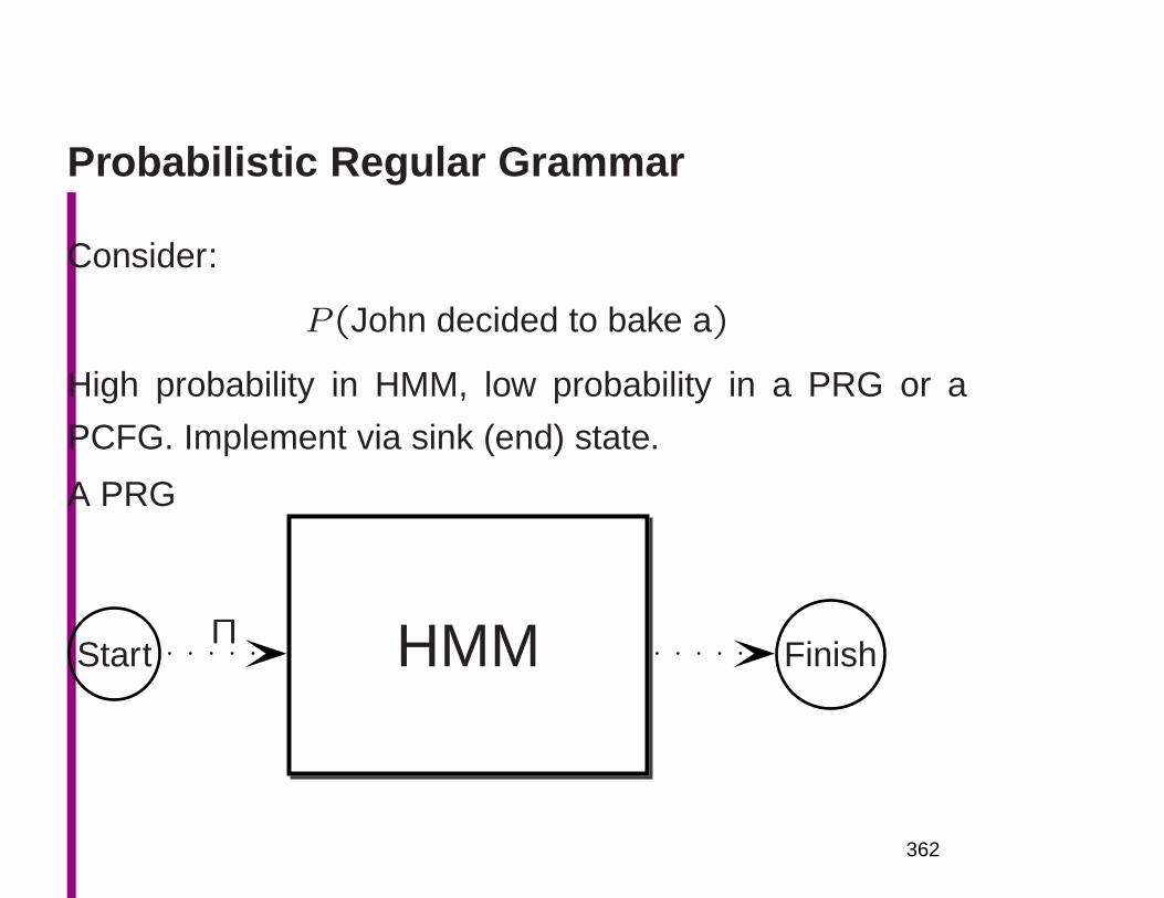
Probabilistic Regular Grammar
Consider:
P (John decided to bake a)
High probability in HMM, low probability in a PRG or a
PCFG. Implement via sink (end) state.
A PRG
Start HMM FinishΠ
362
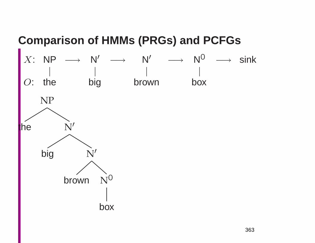
Comparison of HMMs (PRGs) and PCFGs
X: NP −→ N′ −→ N′ −→ N0 −→ sink| | | |
O: the big brown box
NP
the N′
big N′
brown N0
box
363
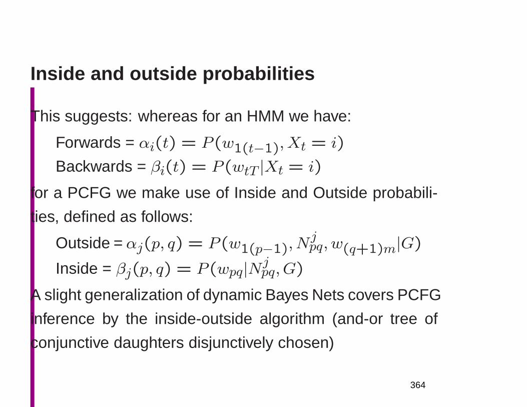
Inside and outside probabilities
This suggests: whereas for an HMM we have:
Forwards = αi(t) = P (w1(t−1), Xt = i)
Backwards = βi(t) = P (wtT |Xt = i)
for a PCFG we make use of Inside and Outside probabili-
ties, defined as follows:
Outside = αj(p, q) = P (w1(p−1), Njpq, w(q+1)m|G)
Inside = βj(p, q) = P (wpq|Njpq, G)
A slight generalization of dynamic Bayes Nets covers PCFG
inference by the inside-outside algorithm (and-or tree of
conjunctive daughters disjunctively chosen)
364
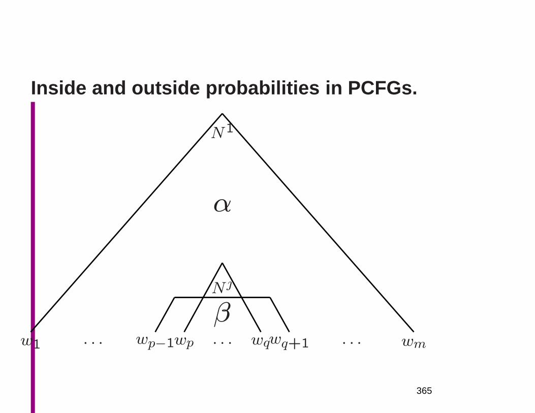
Inside and outside probabilities in PCFGs.
w1 wmwp−1wp wqwq+1
N1
Nj
· · · · · · · · ·
α
β
365
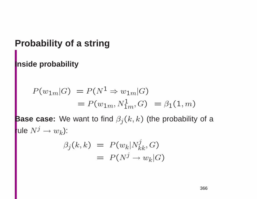
Probability of a string
Inside probability
P (w1m|G) = P (N1 ⇒ w1m|G)
= P (w1m, N11m, G) = β1(1,m)
Base case: We want to find βj(k, k) (the probability of a
rule Nj → wk):
βj(k, k) = P (wk|Njkk, G)
= P (Nj → wk|G)
366

Induction: We want to find βj(p, q), for p < q. As this is the inductivestep using a Chomsky Normal Form grammar, the first rule must be ofthe form Nj → Nr Ns, so we can proceed by induction, dividing thestring in two in various places and summing the result:
Nj
Nr
wp wd
Ns
wd+1 wq
These inside probabilities can be calculated bottom up.
367
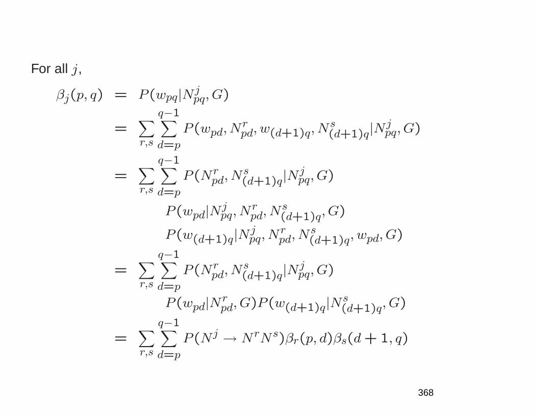
For all j,
βj(p, q) = P(wpq|Njpq, G)
=∑
r,s
q−1∑
d=p
P(wpd, Nrpd, w(d+1)q, N
s(d+1)q|N
jpq, G)
=∑
r,s
q−1∑
d=p
P(Nrpd, N
s(d+1)q|N
jpq, G)
P(wpd|Njpq, N
rpd, N
s(d+1)q, G)
P(w(d+1)q|Njpq, N
rpd, N
s(d+1)q, wpd, G)
=∑
r,s
q−1∑
d=p
P(Nrpd, N
s(d+1)q|N
jpq, G)
P(wpd|Nrpd, G)P(w(d+1)q|Ns
(d+1)q, G)
=∑
r,s
q−1∑
d=p
P(Nj → NrNs)βr(p, d)βs(d+ 1, q)
368
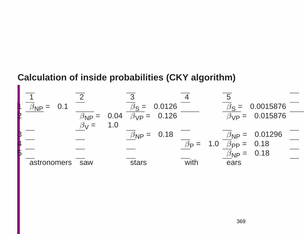
Calculation of inside probabilities (CKY algorithm)
1 2 3 4 51 βNP = 0.1 βS = 0.0126 βS = 0.00158762 βNP = 0.04
βV = 1.0βVP = 0.126 βVP = 0.015876
3 βNP = 0.18 βNP = 0.012964 βP = 1.0 βPP = 0.185 βNP = 0.18
astronomers saw stars with ears
369
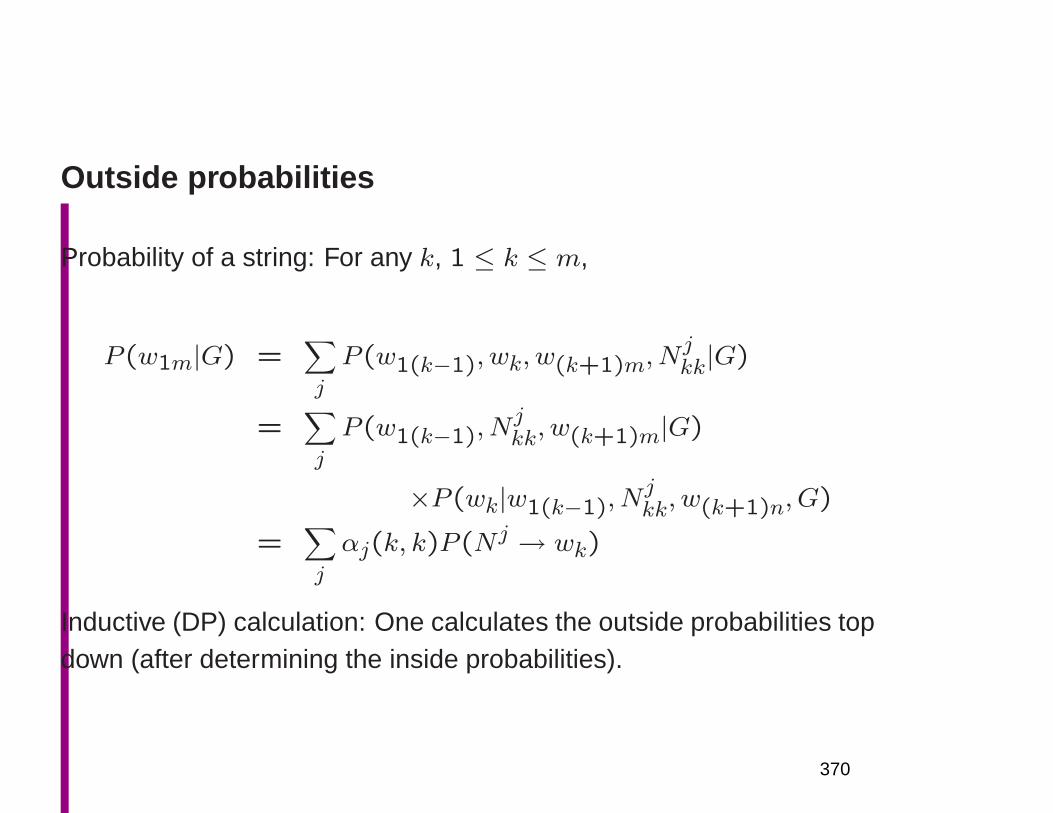
Outside probabilities
Probability of a string: For any k, 1 ≤ k ≤ m,
P(w1m|G) =∑
j
P(w1(k−1), wk, w(k+1)m, Njkk|G)
=∑
j
P(w1(k−1), Njkk, w(k+1)m|G)
×P(wk|w1(k−1), Njkk, w(k+1)n, G)
=∑
j
αj(k, k)P(Nj → wk)
Inductive (DP) calculation: One calculates the outside probabilities topdown (after determining the inside probabilities).
370
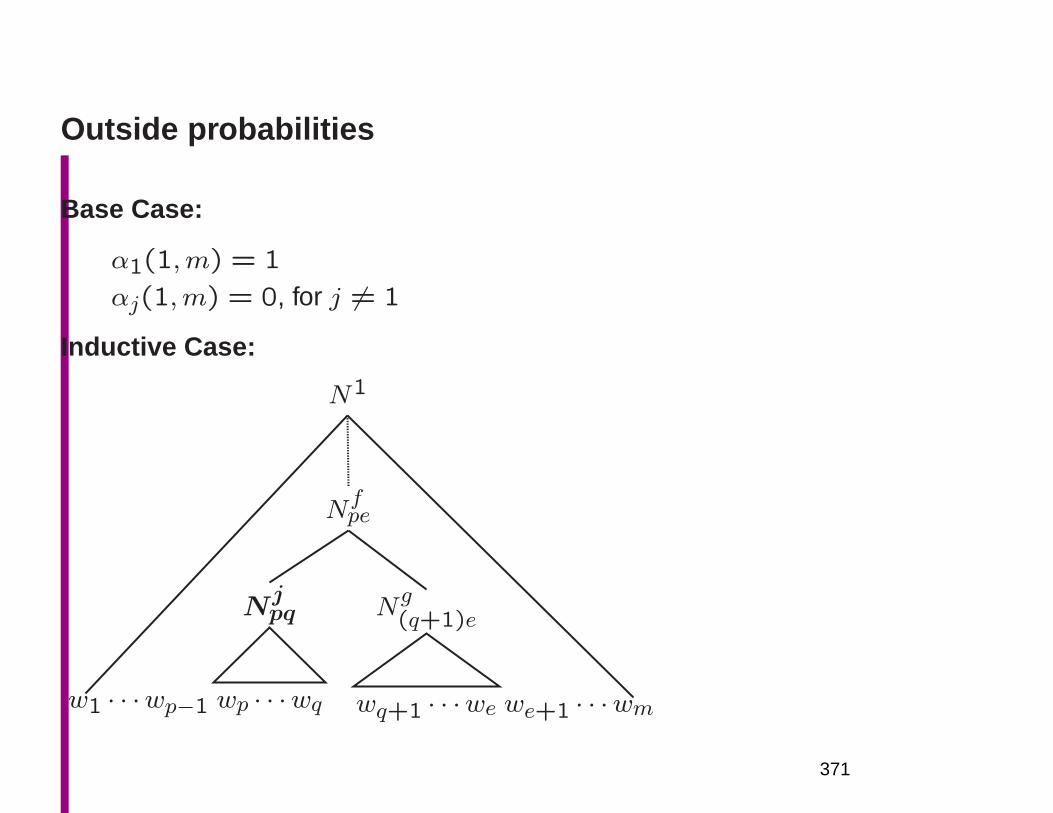
Outside probabilities
Base Case:
α1(1,m) = 1
αj(1,m) = 0, for j 6= 1
Inductive Case:
N1
Nfpe
Njpq
w1 · · ·wp−1 wp · · ·wq
Ng(q+1)e
wq+1 · · ·we we+1 · · ·wm
371

Outside probabilities
Base Case:
α1(1,m) = 1
αj(1,m) = 0, for j 6= 1
Inductive Case: it’s either a left or right branch – we will some overboth possibilities and calculate using outside and inside probabilities
N1
Nfpe
Njpq
w1 · · ·wp−1 wp · · ·wq
Ng(q+1)e
wq+1 · · ·we we+1 · · ·wm
372
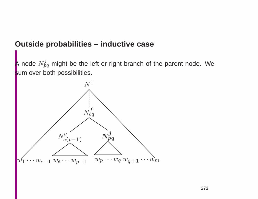
Outside probabilities – inductive case
A node Njpq might be the left or right branch of the parent node. We
sum over both possibilities.
N1
Nfeq
Nge(p−1)
w1 · · ·we−1 we · · ·wp−1
Njpq
wp · · ·wq wq+1 · · ·wm
373
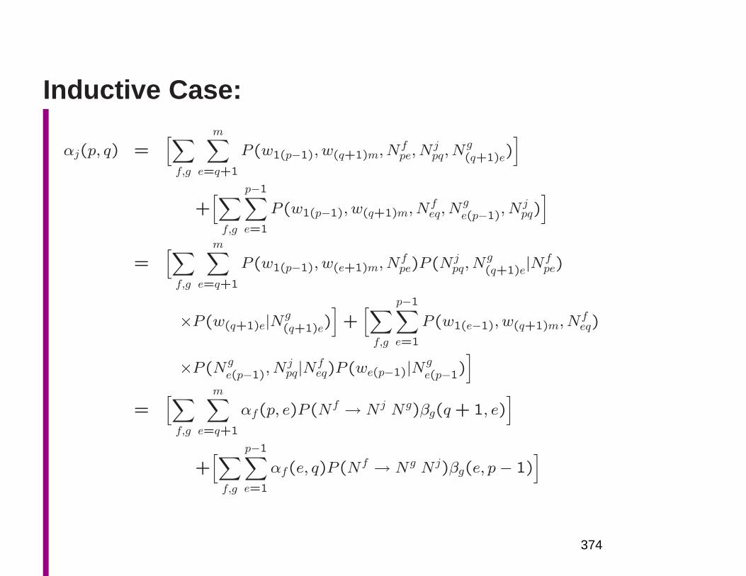
Inductive Case:
αj(p, q) =[
∑
f,g
m∑
e=q+1
P (w1(p−1), w(q+1)m, Nfpe, N
jpq, N
g(q+1)e)
]
+[
∑
f,g
p−1∑
e=1
P (w1(p−1), w(q+1)m, Nfeq, N
ge(p−1)
, N jpq)
]
=[
∑
f,g
m∑
e=q+1
P (w1(p−1), w(e+1)m, Nfpe)P (N j
pq, Ng(q+1)e
|Nfpe)
×P (w(q+1)e|Ng(q+1)e)
]
+[
∑
f,g
p−1∑
e=1
P (w1(e−1), w(q+1)m, Nfeq)
×P (Nge(p−1)
, N jpq|Nf
eq)P (we(p−1)|Nge(p−1)
]
=[
∑
f,g
m∑
e=q+1
αf(p, e)P (Nf → N j Ng)βg(q+ 1, e)]
+[
∑
f,g
p−1∑
e=1
αf(e, q)P (Nf → Ng N j)βg(e, p− 1)]
374
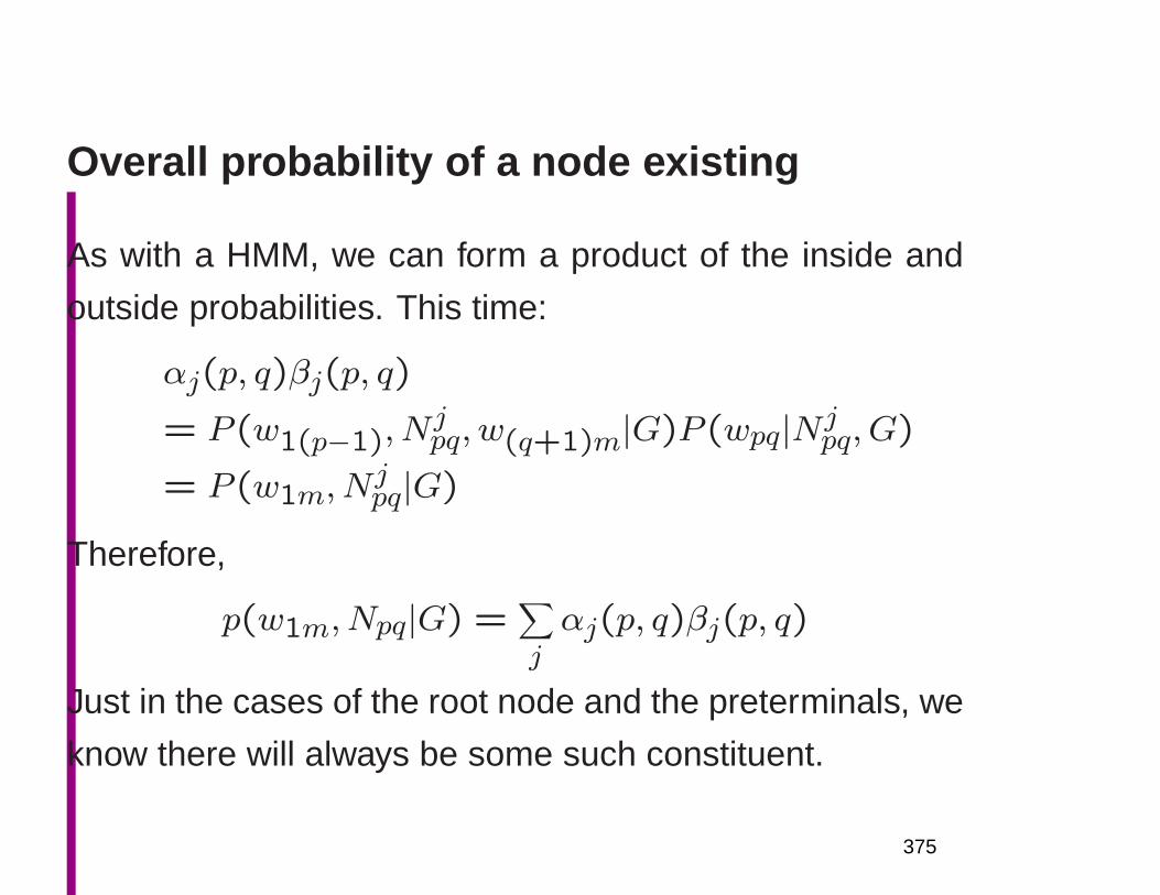
Overall probability of a node existing
As with a HMM, we can form a product of the inside and
outside probabilities. This time:
αj(p, q)βj(p, q)
= P (w1(p−1), Njpq, w(q+1)m|G)P (wpq|Nj
pq, G)
= P (w1m, Njpq|G)
Therefore,
p(w1m, Npq|G) =∑
jαj(p, q)βj(p, q)
Just in the cases of the root node and the preterminals, we
know there will always be some such constituent.
375
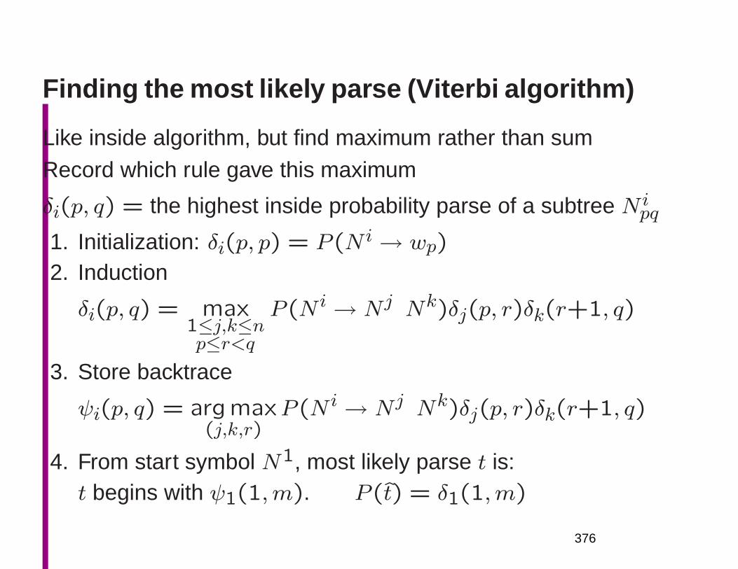
Finding the most likely parse (Viterbi algorithm)
Like inside algorithm, but find maximum rather than sum
Record which rule gave this maximum
δi(p, q) = the highest inside probability parse of a subtree N ipq
1. Initialization: δi(p, p) = P (N i→ wp)
2. Induction
δi(p, q) = max1≤j,k≤np≤r<q
P (N i→ Nj Nk)δj(p, r)δk(r+1, q)
3. Store backtrace
ψi(p, q) = argmax(j,k,r)
P (N i→ Nj Nk)δj(p, r)δk(r+1, q)
4. From start symbol N1, most likely parse t is:t begins with ψ1(1,m). P (t) = δ1(1,m)
376
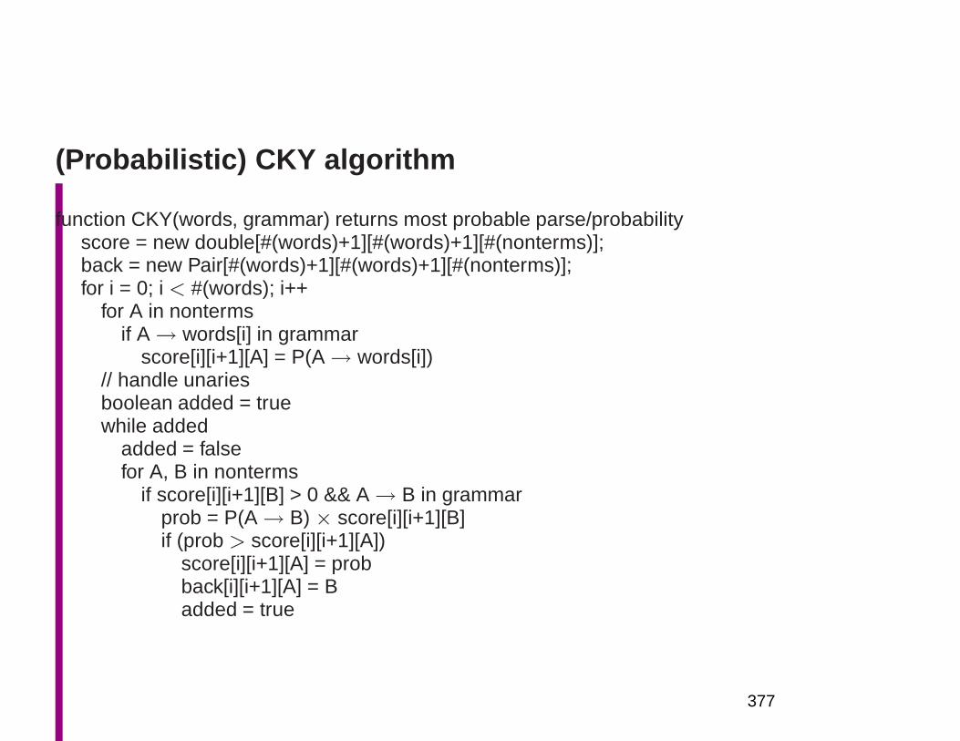
(Probabilistic) CKY algorithm
function CKY(words, grammar) returns most probable parse/probabilityscore = new double[#(words)+1][#(words)+1][#(nonterms)];back = new Pair[#(words)+1][#(words)+1][#(nonterms)];for i = 0; i < #(words); i++
for A in nontermsif A→ words[i] in grammar
score[i][i+1][A] = P(A→ words[i])// handle unariesboolean added = truewhile added
added = falsefor A, B in nonterms
if score[i][i+1][B] > 0 && A→ B in grammarprob = P(A→ B) × score[i][i+1][B]if (prob > score[i][i+1][A])
score[i][i+1][A] = probback[i][i+1][A] = Badded = true
377
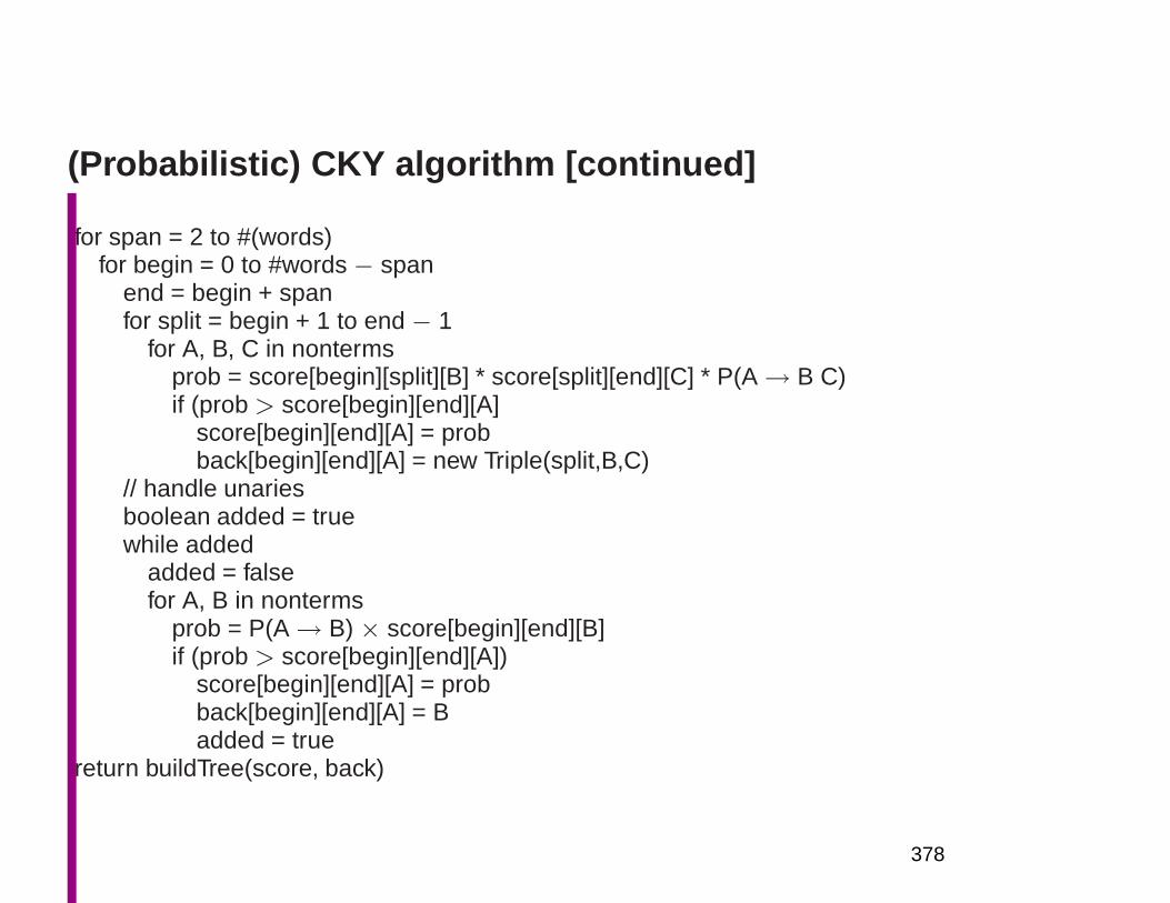
(Probabilistic) CKY algorithm [continued]
for span = 2 to #(words)for begin = 0 to #words − span
end = begin + spanfor split = begin + 1 to end − 1
for A, B, C in nontermsprob = score[begin][split][B] * score[split][end][C] * P(A→ B C)if (prob > score[begin][end][A]
score[begin][end][A] = probback[begin][end][A] = new Triple(split,B,C)
// handle unariesboolean added = truewhile added
added = falsefor A, B in nonterms
prob = P(A→ B) × score[begin][end][B]if (prob > score[begin][end][A])
score[begin][end][A] = probback[begin][end][A] = Badded = true
return buildTree(score, back)
378
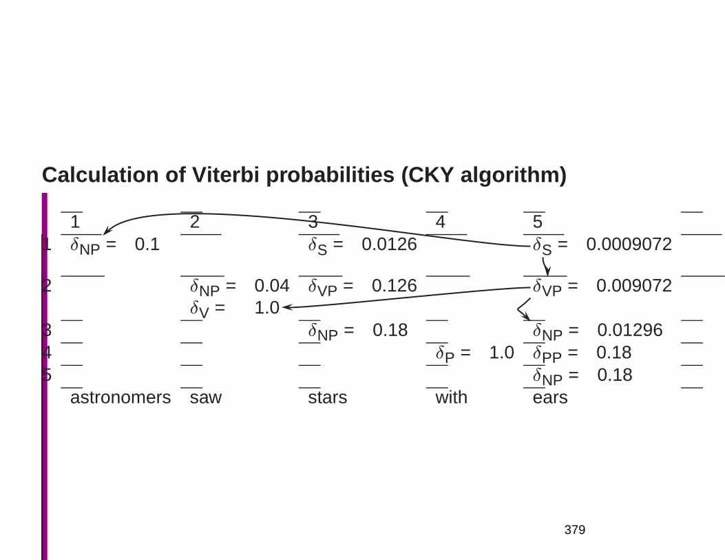
Calculation of Viterbi probabilities (CKY algorithm)
1 2 3 4 51 δNP = 0.1 δS = 0.0126 δS = 0.0009072
2 δNP = 0.04δV = 1.0
δVP = 0.126 δVP = 0.009072
3 δNP = 0.18 δNP = 0.012964 δP = 1.0 δPP = 0.185 δNP = 0.18
astronomers saw stars with ears
379
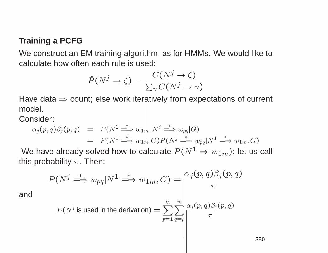
Training a PCFG
We construct an EM training algorithm, as for HMMs. We would like tocalculate how often each rule is used:
P (Nj → ζ) =C(Nj → ζ)
∑
γ C(Nj → γ)
Have data⇒ count; else work iteratively from expectations of currentmodel.Consider:
αj(p, q)βj(p, q) = P (N1 ∗=⇒ w1m, N
j ∗=⇒ wpq|G)
= P (N1 ∗=⇒ w1m|G)P (N j ∗
=⇒ wpq|N1 ∗=⇒ w1m, G)
We have already solved how to calculate P(N1 ⇒ w1m); let us callthis probability π. Then:
P(Nj ∗=⇒ wpq|N1 ∗
=⇒ w1m, G) =αj(p, q)βj(p, q)
πand
E(N j is used in the derivation) =
m∑
p=1
m∑
q=p
αj(p, q)βj(p, q)
π
380
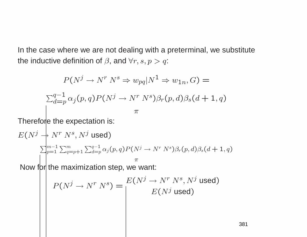
In the case where we are not dealing with a preterminal, we substitutethe inductive definition of β, and ∀r, s, p > q:
P(Nj → Nr Ns ⇒ wpq|N1 ⇒ w1n, G) =
∑q−1d=pαj(p, q)P(Nj → Nr Ns)βr(p, d)βs(d+ 1, q)
π
Therefore the expectation is:
E(Nj → Nr Ns, Nj used)∑m−1
p=1
∑mq=p+1
∑q−1d=p αj(p, q)P (N j → N r N s)βr(p, d)βs(d+ 1, q)
π
Now for the maximization step, we want:
P(Nj → Nr Ns) =E(Nj → Nr Ns, Nj used)
E(Nj used)
381
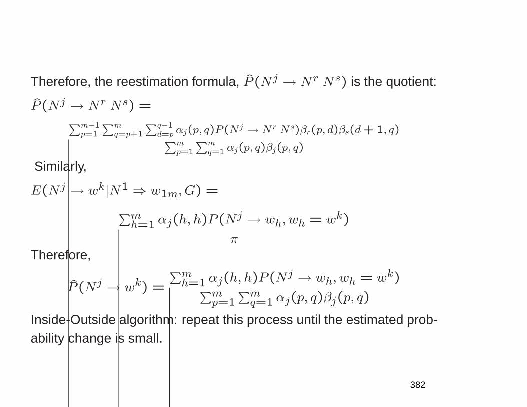
Therefore, the reestimation formula, P (Nj → Nr Ns) is the quotient:
P (Nj → Nr Ns) =∑m−1
p=1
∑mq=p+1
∑q−1d=p αj(p, q)P (N j → N r N s)βr(p, d)βs(d+ 1, q)∑m
p=1
∑mq=1 αj(p, q)βj(p, q)
Similarly,
E(Nj → wk|N1 ⇒ w1m, G) =
∑mh=1αj(h, h)P(Nj → wh, wh = wk)
πTherefore,
P (Nj → wk) =
∑mh=1 αj(h, h)P(Nj → wh, wh = wk)
∑mp=1
∑mq=1 αj(p, q)βj(p, q)
Inside-Outside algorithm: repeat this process until the estimated prob-ability change is small.
382
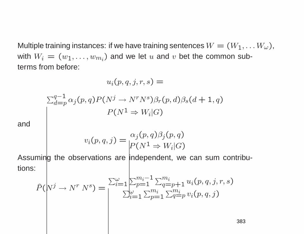
Multiple training instances: if we have training sentencesW = (W1, . . .Wω),with Wi = (w1, . . . , wmi) and we let u and v bet the common sub-terms from before:
ui(p, q, j, r, s) =
∑q−1d=pαj(p, q)P(Nj → NrNs)βr(p, d)βs(d+ 1, q)
P(N1 ⇒Wi|G)
and
vi(p, q, j) =αj(p, q)βj(p, q)
P(N1 ⇒Wi|G)
Assuming the observations are independent, we can sum contribu-tions:
P (Nj → Nr Ns) =
∑ωi=1
∑mi−1p=1
∑miq=p+1 ui(p, q, j, r, s)
∑ωi=1
∑mip=1
∑miq=p vi(p, q, j)
383
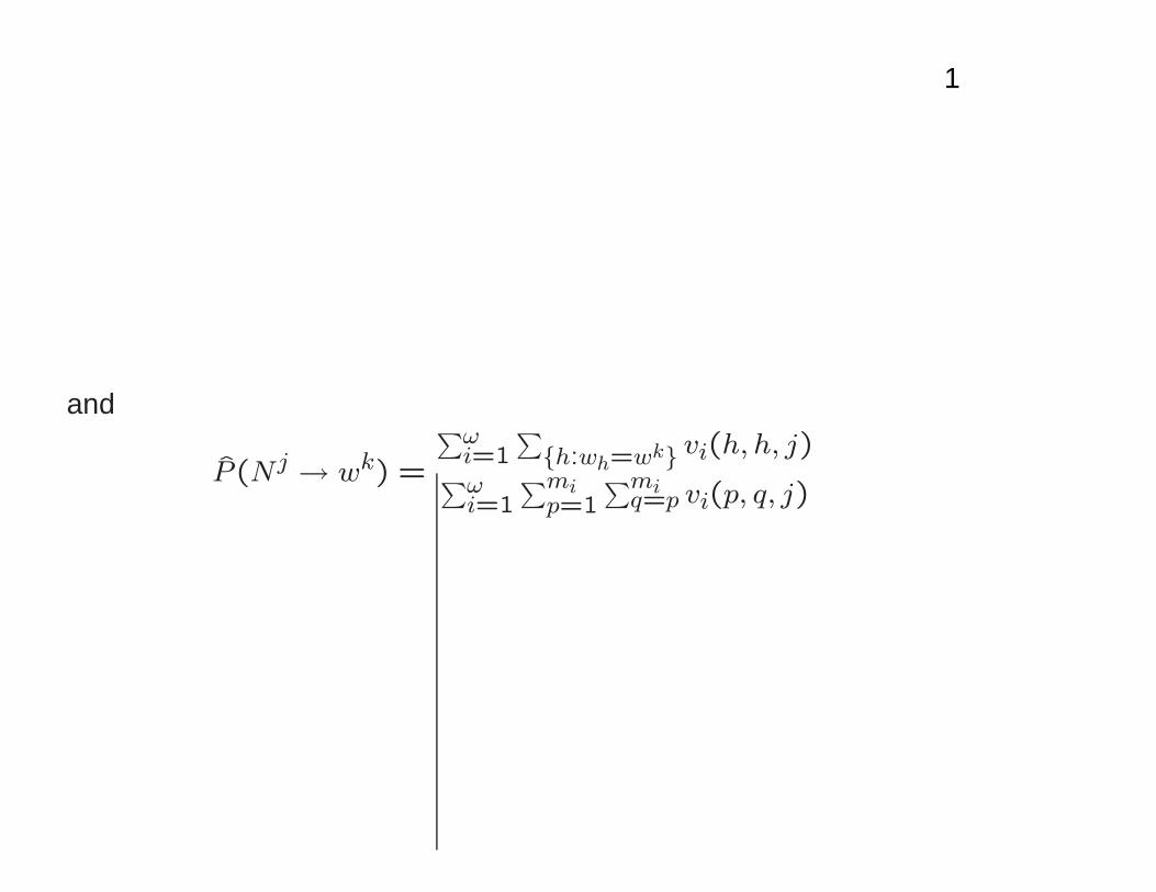
1
and
P (Nj → wk) =
∑ωi=1
∑
h:wh=wk vi(h, h, j)∑ωi=1
∑mip=1
∑miq=p vi(p, q, j)

Variant slides
384
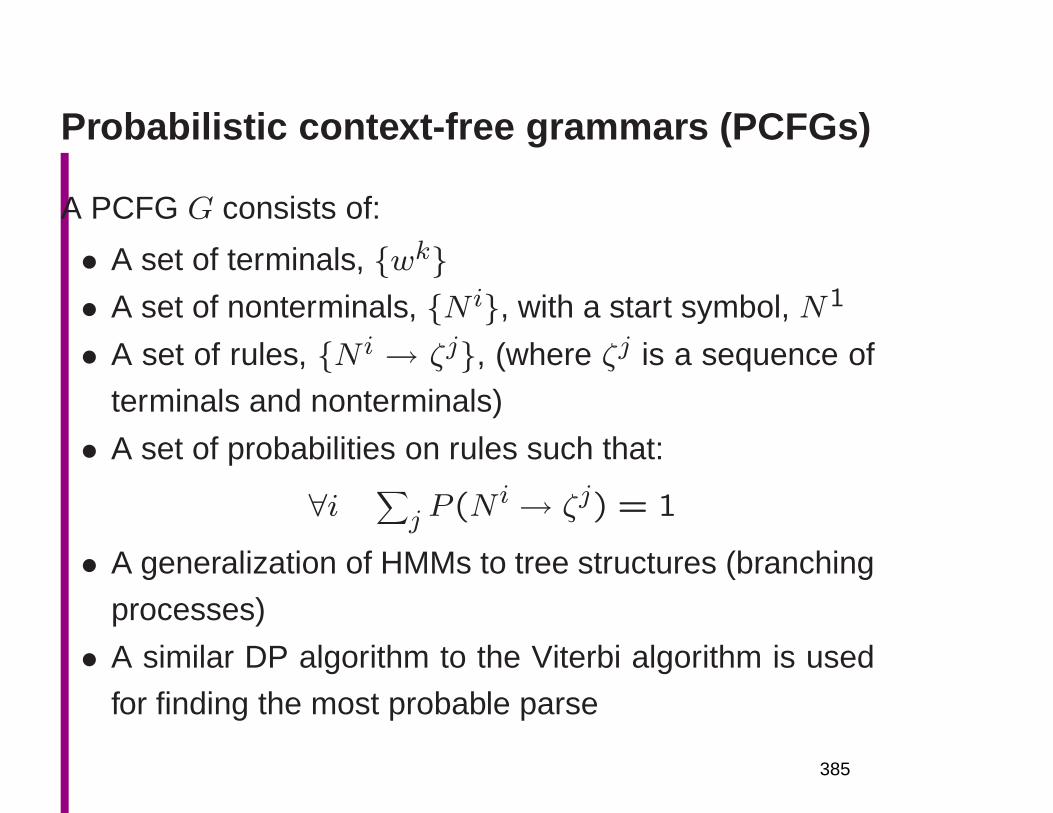
Probabilistic context-free grammars (PCFGs)
A PCFG G consists of:
• A set of terminals, wk• A set of nonterminals, N i, with a start symbol, N1
• A set of rules, N i → ζj, (where ζj is a sequence of
terminals and nonterminals)
• A set of probabilities on rules such that:
∀i ∑
j P (N i→ ζj) = 1
• A generalization of HMMs to tree structures (branching
processes)
• A similar DP algorithm to the Viterbi algorithm is used
for finding the most probable parse
385
PCFGs
• Like a regular CFG but put probability on each rule
• Probabilities are also completely context-free, depend-
ing just on parent node
• Just as for HMMs, there are three basic questions we
wish to answer:
– P (w1m|G)
– argmaxtP (t|w1m, G)
– Learning algorithm. Find G such that P (w1m|G) is
maximized.
386
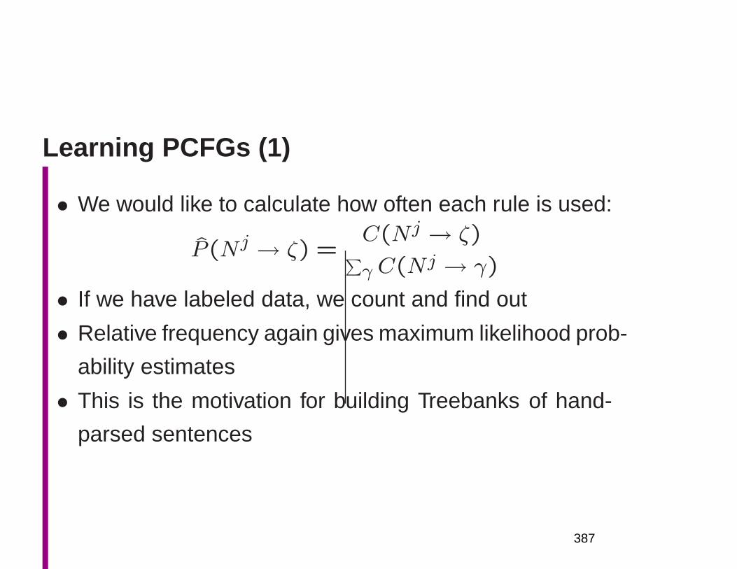
Learning PCFGs (1)
• We would like to calculate how often each rule is used:
P (Nj → ζ) =C(Nj → ζ)
∑
γ C(Nj → γ)
• If we have labeled data, we count and find out
• Relative frequency again gives maximum likelihood prob-
ability estimates
• This is the motivation for building Treebanks of hand-
parsed sentences
387
Learning PCFGs (2): the Inside-Outside algo-rithm (Baker 1979)
• Otherwise we work iteratively from expectations of cur-
rent model.
• We construct an EM training algorithm, as for HMMs
• For each sentence, at each iteration, we work out ex-
pectation of how often each rule is used using inside
and outside probabilities
• We assume sentences are independent and sum ex-
pectations over parses of each
• We re-estimate rules based on these ‘counts’
388
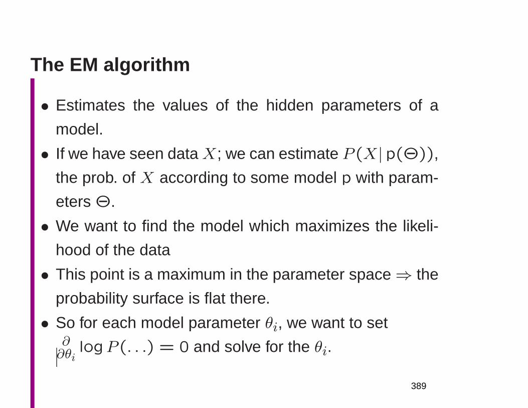
The EM algorithm
• Estimates the values of the hidden parameters of a
model.
• If we have seen dataX; we can estimate P (X|p(Θ)),
the prob. of X according to some model p with param-
eters Θ.
• We want to find the model which maximizes the likeli-
hood of the data
• This point is a maximum in the parameter space⇒ the
probability surface is flat there.
• So for each model parameter θi, we want to set∂∂θi
logP (. . .) = 0 and solve for the θi.
389
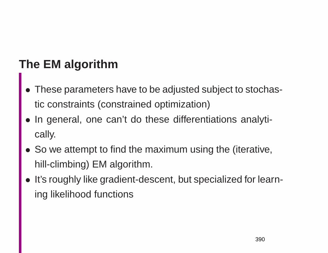
The EM algorithm
• These parameters have to be adjusted subject to stochas-
tic constraints (constrained optimization)
• In general, one can’t do these differentiations analyti-
cally.
• So we attempt to find the maximum using the (iterative,
hill-climbing) EM algorithm.
• It’s roughly like gradient-descent, but specialized for learn-
ing likelihood functions
390
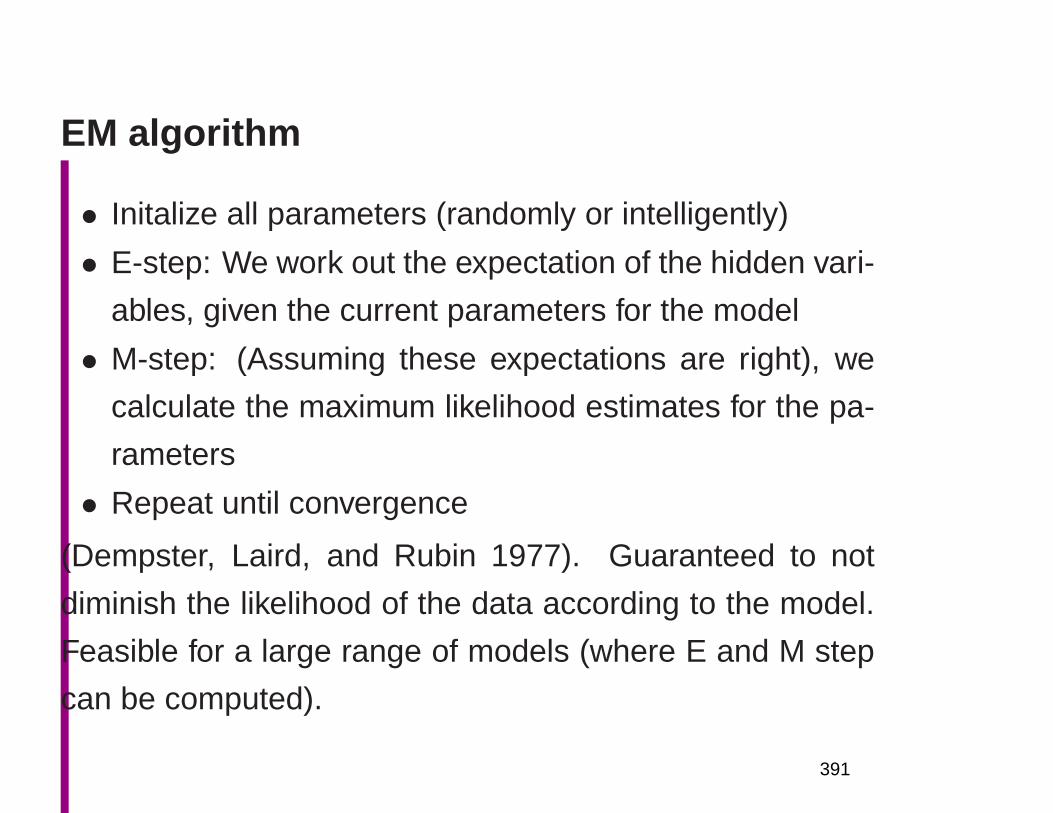
EM algorithm
• Initalize all parameters (randomly or intelligently)
• E-step: We work out the expectation of the hidden vari-
ables, given the current parameters for the model
• M-step: (Assuming these expectations are right), we
calculate the maximum likelihood estimates for the pa-
rameters
• Repeat until convergence
(Dempster, Laird, and Rubin 1977). Guaranteed to not
diminish the likelihood of the data according to the model.
Feasible for a large range of models (where E and M step
can be computed).
391
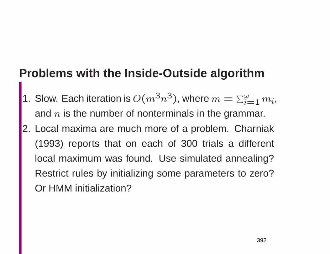
Problems with the Inside-Outside algorithm
1. Slow. Each iteration isO(m3n3), wherem =∑ωi=1mi,
and n is the number of nonterminals in the grammar.
2. Local maxima are much more of a problem. Charniak
(1993) reports that on each of 300 trials a different
local maximum was found. Use simulated annealing?
Restrict rules by initializing some parameters to zero?
Or HMM initialization?
392
Problems with the Inside-Outside algorithm
3. Lari and Young (1990) suggest that you need many
more nonterminals available than are theoretically nec-
essary to get good grammar learning (about a threefold
increase?). This compounds the first problem.
4. There is no guarantee that the nonterminals that the
algorithm learns will have any satisfactory resemblance
to the kinds of nonterminals normally motivated in lin-
guistic analysis (NP, VP, etc.).
393
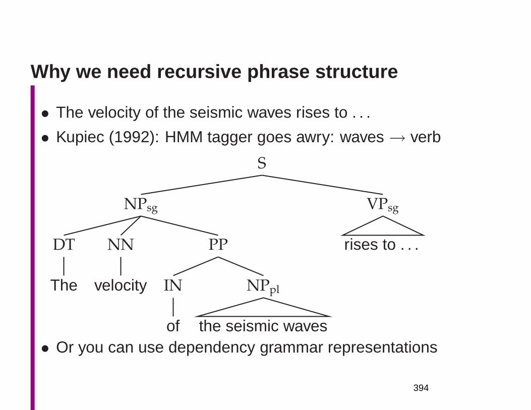
Why we need recursive phrase structure
• The velocity of the seismic waves rises to . . .
• Kupiec (1992): HMM tagger goes awry: waves→ verb
S
NPsg
DT
The
NN
velocity
PP
IN
of
NPpl
the seismic waves
VPsg
rises to . . .
• Or you can use dependency grammar representations
394
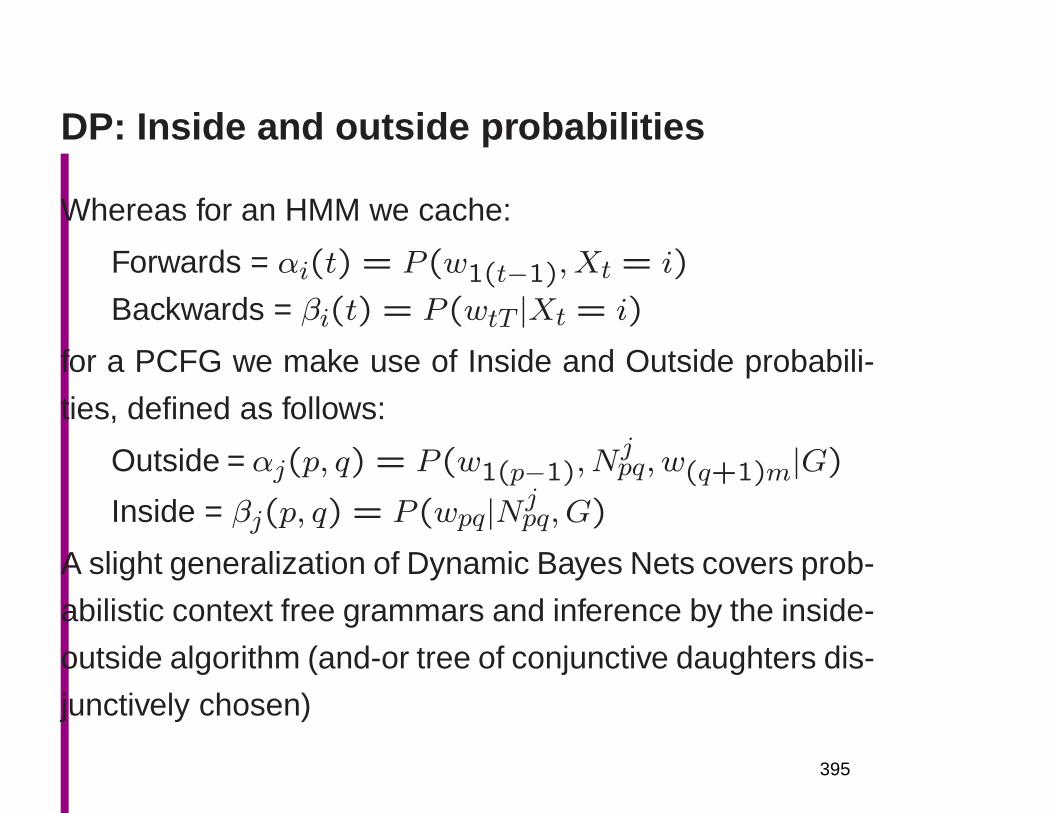
DP: Inside and outside probabilities
Whereas for an HMM we cache:
Forwards = αi(t) = P (w1(t−1), Xt = i)
Backwards = βi(t) = P (wtT |Xt = i)
for a PCFG we make use of Inside and Outside probabili-
ties, defined as follows:
Outside = αj(p, q) = P (w1(p−1), Njpq, w(q+1)m|G)
Inside = βj(p, q) = P (wpq|Njpq, G)
A slight generalization of Dynamic Bayes Nets covers prob-
abilistic context free grammars and inference by the inside-
outside algorithm (and-or tree of conjunctive daughters dis-
junctively chosen)
395
2. Complex NLP Case Study:Question Answering
• Task is a long pipeline of many subtasks
• Task seems AI complete
• NLP offers compelling performance advantages over
IR-style techniques
• But still lots of room for improvement
396

Question answering from text
• TREC 8/9 QA competition: an idea originating from theIR community
• With massive collections of on-line documents, manualtranslation of textual information into knowledge basescovering large numbers of domains is impractical: Wewant to answer questions from textbases
• Evaluated output is 5 answers of 50/250 byte snippetsof text drawn from a 3 GB text collection, and requiredto contain at least one concept of the semantic cate-gory of the expected answer type. (IR think. Suggeststhe use of named entity recognizers.)
• Get reciprocal points for highest correct answer.
397

IBM
TJ W
atsonIB
M T
J Watson
LCC
-SM
UU
niv. of Waterloo
Queens C
ollegeK
orea Univ.
Syracuse U
niv.Im
perial CollegeN
TT
Alicante U
niv.X
erox Europe
KA
IST
Univ. of S
heffieldM
icrosoft Research
Fudan U
niv.U
niv. of Alberta
Univ. of M
ontrealLIM
SI
CL R
esearchS
eoul Nat. U
niv.P
isaC
oneroxM
ITR
E
0.7
0.6
0.5
0.4
0.3
0.2
0.1
TREC-9 50 bytes
IBM
TJ W
atsonIB
M T
J Watson
LCC
-SM
U
Korea U
niv.
Pisa
0.7
0.6
0.5
0.4
0.3
0.2
0.1
0.8
Queens C
ollegeU
niv. of Waterloo
LIMS
I
NT
TIm
perial College
Syracuse U
niv.U
niv. of Montreal
Alicante U
niv.X
erox Europe
Univ. of S
heffieldS
UN
Univ. of M
arylandF
udan Univ.
KA
IST
Nat. T
aiwan
CL R
esearchM
icrosoft Research
Univ. of Iow
a
MIT
RE
Seoul N
at. Univ.
0
0
US
C/IS
I
TREC-9 250 bytes
398
Pasca and Harabagiu (2001) demonstrates thevalue of sophisticated NLP processing
• Good IR is needed: paragraph retrieval based on SMART
• Large taxonomy of question types and expected an-swer types is crucial
• Statistical parser (modeled on Collins 1997) used toparse questions and relevant text for answers, and tobuild knowledge base
• Controlled query expansion loops (morphological, lexi-cal synonyms, and semantic relations) are all importantin retrieving the correct answer.
• Answer ranking by ML method based on this informa-tion surpasses IR-style empirical methods.
399
Question Answering Example (1)
• Q261: What company sells most greetings cards ?
• sells(ORGANIZATION, cards(greeting), most)
• “Hallmark remains the largest maker of greeting cards”maker(ORGANIZATION(Hallmark), cards(greeting), largest)
• Need an entailment between producing, or making andselling goods
• Derived from WordNet, since synset make, produce,create has the genus manufacture , defined in the gloss
of its nominalization as (for ) sale
• Also, need most ≈ largest
• Therefore the semantic form of question Q261 and its
illustrated answer are similar
400

Question Answering Example (2)
• How hot does the inside of an active volcano get ?
• get(TEMPERATURE, inside(volcano(active)))
• “lava fragments belched out of the mountain were ashot as 300 degrees Fahrenheit”
• fragments(lava, TEMPERATURE(degrees(300)),belched(out, mountain))
• – volcano ISA mountain– lava ISPARTOF volcano lava inside volcano– fragments of lava HAVEPROPERTIESOF lava
• The needed semantic information is available in Word-Net definitions, and was successfully translated into aform that can be used for rough ‘proofs’
401
What’s used where? QA lessons learned
• IR: is not probabilistic, but is thoroughly quantitative,with well-honed, if ad hoc, ranking schemes
• Parsing: probabilistic parser (Collins 1997 clone) – theone big practical success of probabilistic parsing [speechwins (Charniak 2001) are still theoretical].
• Semantic interpretation: all loosely logical (though prob-abilistic parser is used to build knowledge base fromWordNet) – succeeded by aiming low?
• Result ranking: ordering of paragraphs done by a per-ceptron classifier (7 features: question word matches,distance from words to answer type word, punctuationafter answer, etc.). Statistical, but not high tech.
402
PCFGs
• Like a regular CFG but put probability on each rule
• Key independence assumption: Probabilities are also
completely context-free, depending just on parent node
• Allow probabilistic inference:
– P (w1 · · ·wm|G)
– argmaxtP (t|w1 · · ·wm, G)
– Find G such that P (w1 · · ·wm|G) is maximized
• Give a partial solution for resolving grammar ambigui-
ties – but not too good, as not lexicalized
• Better for grammar induction (Gold (1967) vs.Horning
(1969)) and robustness
403
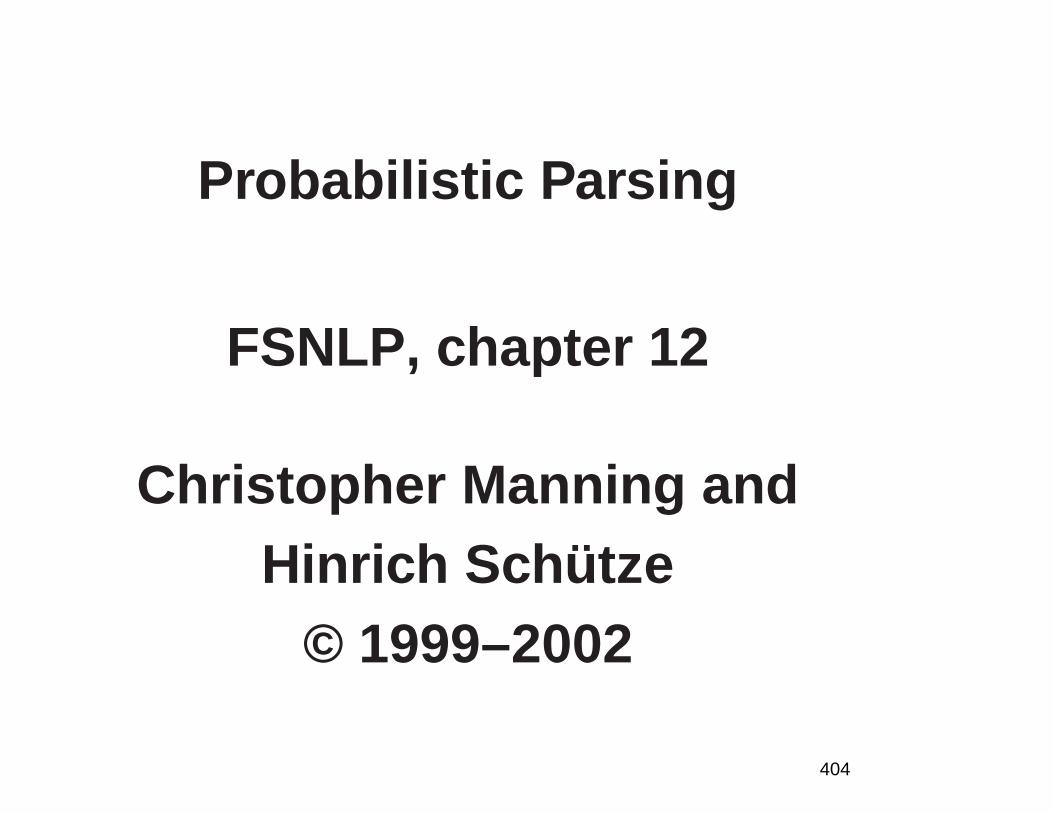
Probabilistic Parsing
FSNLP, chapter 12
Christopher Manning andHinrich Schütze
© 1999–2002
404
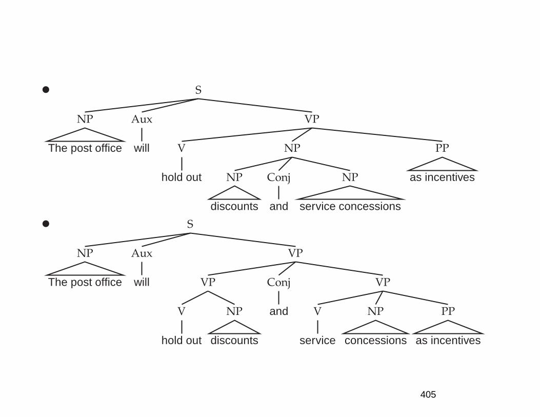
• S
NP
The post office
Aux
will
VP
V
hold out
NP
NP
discounts
Conj
and
NP
service concessions
PP
as incentives
• S
NP
The post office
Aux
will
VP
VP
V
hold out
NP
discounts
Conj
and
VP
V
service
NP
concessions
PP
as incentives
405
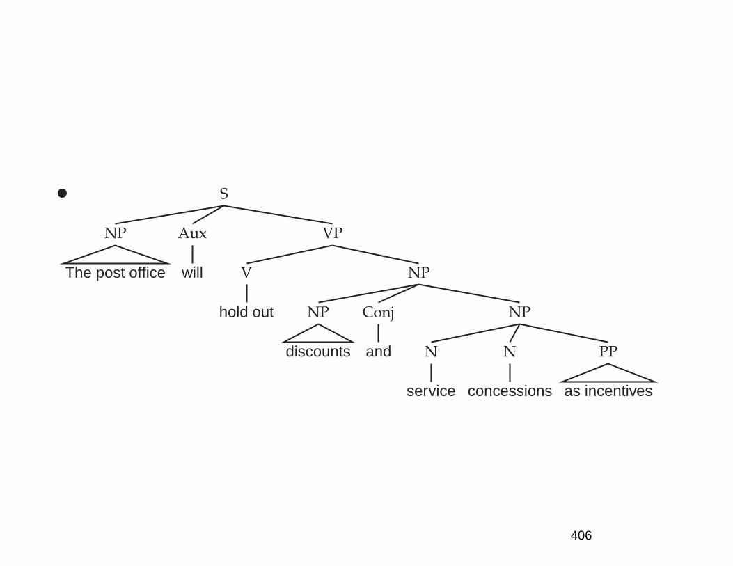
• S
NP
The post office
Aux
will
VP
V
hold out
NP
NP
discounts
Conj
and
NP
N
service
N
concessions
PP
as incentives
406
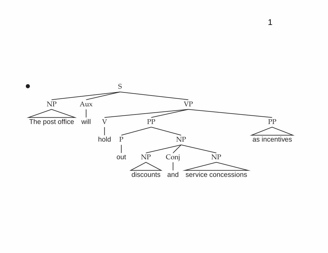
1
• S
NP
The post office
Aux
will
VP
V
hold
PP
P
out
NP
NP
discounts
Conj
and
NP
service concessions
PP
as incentives
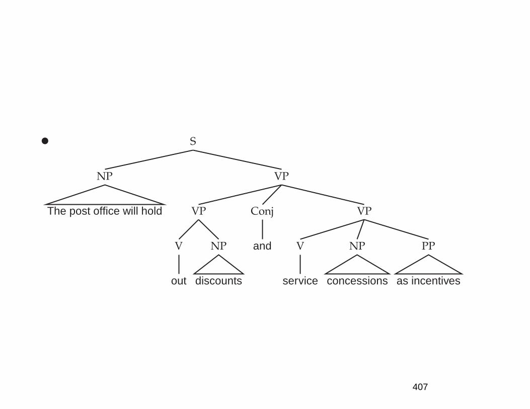
• S
NP
The post office will hold
VP
VP
V
out
NP
discounts
Conj
and
VP
V
service
NP
concessions
PP
as incentives
407

Modern Statistical Parsers
• A greatly increased ability to do accurate, robust, broadcoverage parsing (Charniak 1997; Collins 1997; Ratna-parkhi 1997b; Charniak 2000; Charniak and Johnson2005)• Achieved by converting parsing into a classification task
and using statistical/machine learning methods• Statistical methods (fairly) accurately resolve structural
and real world ambiguities• Much faster: rather than being cubic in the sentence
length or worse, many statistical parsers parse in lineartime (by using beam search)• Provide probabilistic language models that can be inte-
grated with speech recognition systems.
408
Supervised ML parsing
• The crucial resource has been treebanks of parses,
especially the Penn Treebank (Marcus et al. 1993)
• From these, we train classifiers:
– Mainly probabilistic models, but also:
– Conventional decision trees
– Decision lists/transformation-based learning
• Possible only when extensive resources exist
• Somewhat uninteresting from Cog. Sci. viewpoint – which
would prefer bootstrapping from minimal supervision
409
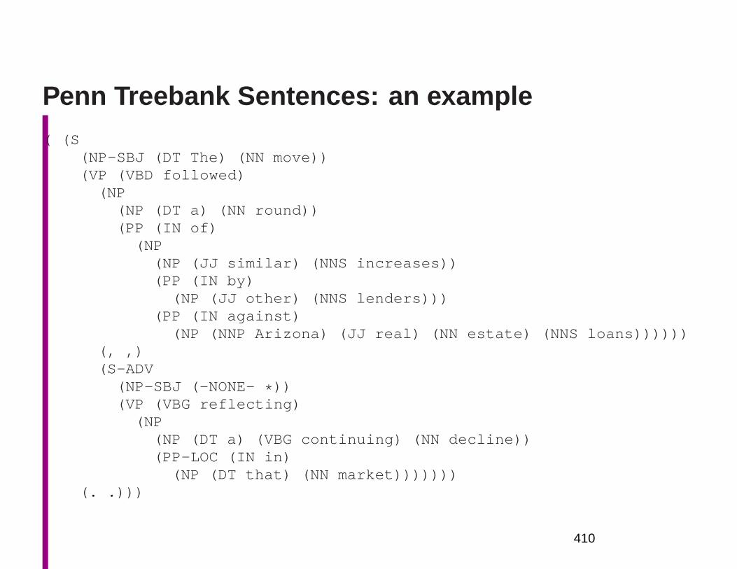
Penn Treebank Sentences: an example( (S
(NP-SBJ (DT The) (NN move))(VP (VBD followed)
(NP(NP (DT a) (NN round))(PP (IN of)
(NP(NP (JJ similar) (NNS increases))(PP (IN by)
(NP (JJ other) (NNS lenders)))(PP (IN against)
(NP (NNP Arizona) (JJ real) (NN estate) (NNS loans))))))(, ,)(S-ADV
(NP-SBJ (-NONE- * ))(VP (VBG reflecting)
(NP(NP (DT a) (VBG continuing) (NN decline))(PP-LOC (IN in)
(NP (DT that) (NN market)))))))(. .)))
410
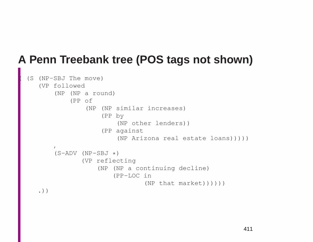
A Penn Treebank tree (POS tags not shown)( (S (NP-SBJ The move)
(VP followed(NP (NP a round)
(PP of(NP (NP similar increases)
(PP by(NP other lenders))
(PP against(NP Arizona real estate loans)))))
,(S-ADV (NP-SBJ * )
(VP reflecting(NP (NP a continuing decline)
(PP-LOC in(NP that market))))))
.))
411
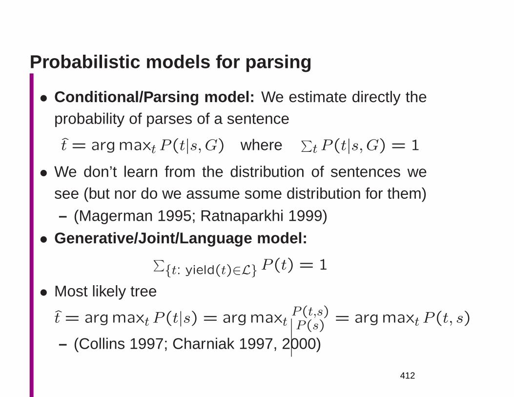
Probabilistic models for parsing
• Conditional/Parsing model: We estimate directly theprobability of parses of a sentence
t = argmaxtP (t|s,G) where∑
tP (t|s,G) = 1
• We don’t learn from the distribution of sentences wesee (but nor do we assume some distribution for them)– (Magerman 1995; Ratnaparkhi 1999)
• Generative/Joint/Language model:∑
t: yield(t)∈L P (t) = 1
• Most likely tree
t = argmaxtP (t|s) = argmaxtP(t,s)P(s)
= argmaxtP (t, s)
– (Collins 1997; Charniak 1997, 2000)
412
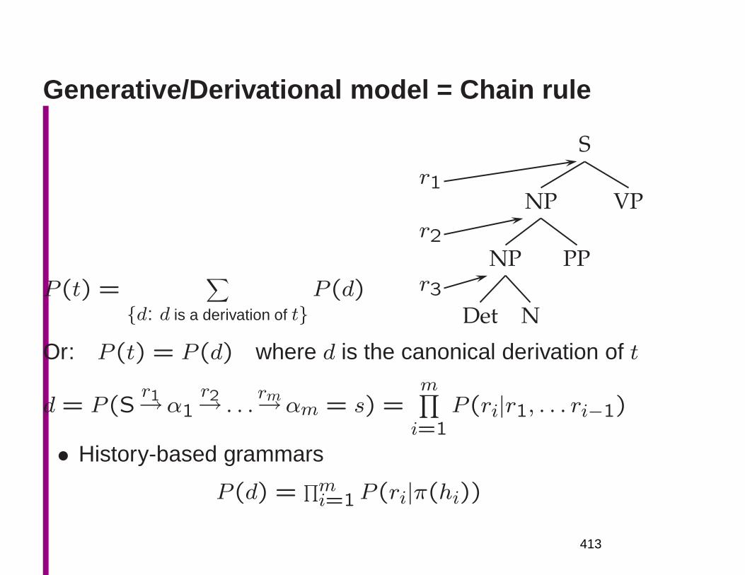
Generative/Derivational model = Chain rule
P (t) =∑
d: d is a derivation of tP (d)
r1
r2
r3
S
NP
NP
Det N
PP
VP
Or: P (t) = P (d) where d is the canonical derivation of t
d = P (Sr1→α1
r2→ . . .rm→αm = s) =
m∏
i=1P (ri|r1, . . . ri−1)
• History-based grammars
P (d) =∏mi=1P (ri|π(hi))
413
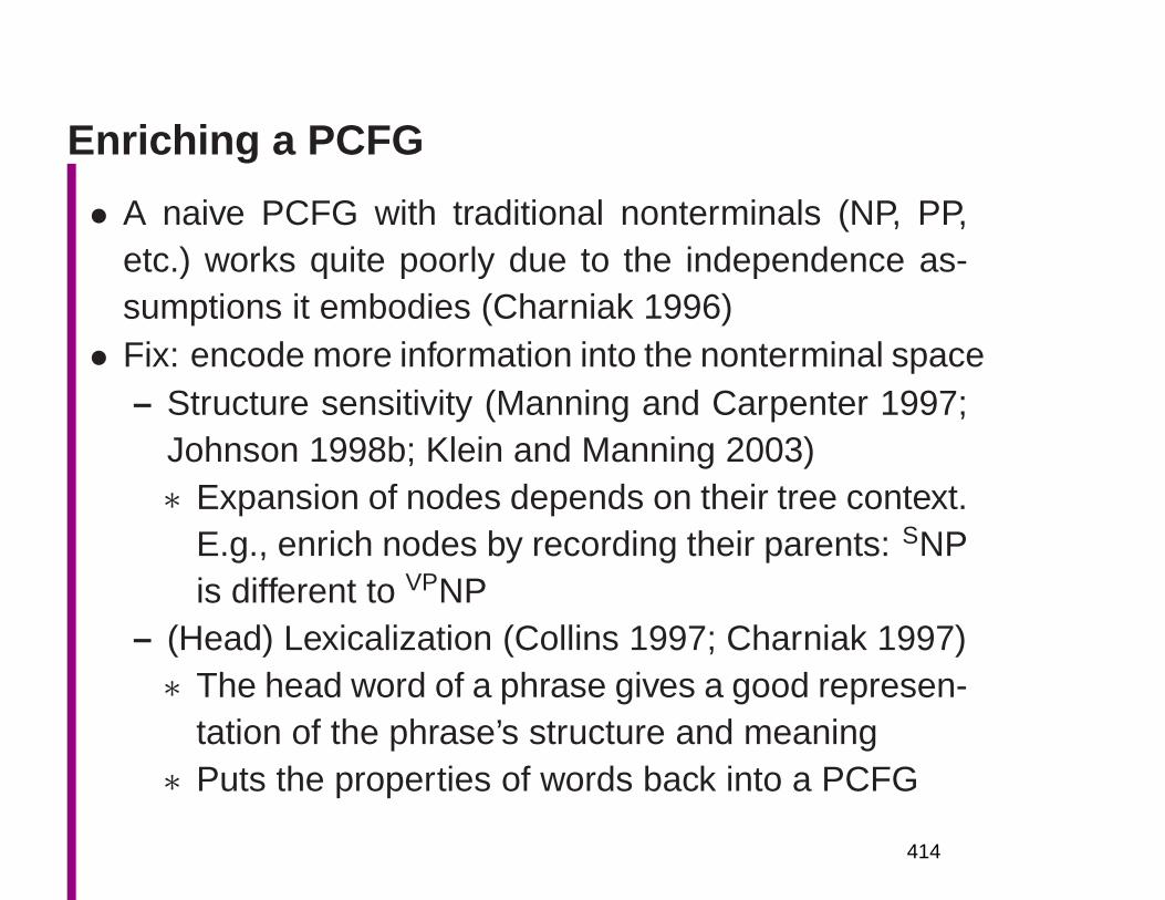
Enriching a PCFG
• A naive PCFG with traditional nonterminals (NP, PP,etc.) works quite poorly due to the independence as-sumptions it embodies (Charniak 1996)• Fix: encode more information into the nonterminal space
– Structure sensitivity (Manning and Carpenter 1997;Johnson 1998b; Klein and Manning 2003)∗ Expansion of nodes depends on their tree context.
E.g., enrich nodes by recording their parents: SNPis different to VPNP
– (Head) Lexicalization (Collins 1997; Charniak 1997)∗ The head word of a phrase gives a good represen-
tation of the phrase’s structure and meaning∗ Puts the properties of words back into a PCFG
414
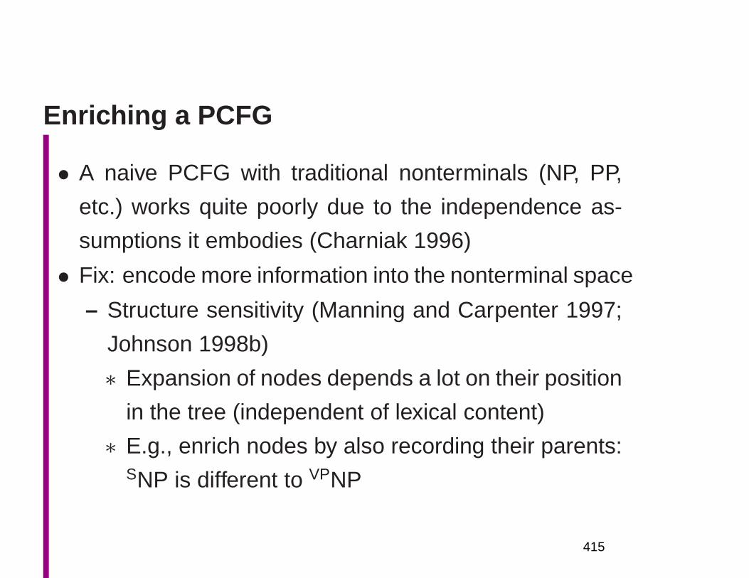
Enriching a PCFG
• A naive PCFG with traditional nonterminals (NP, PP,
etc.) works quite poorly due to the independence as-
sumptions it embodies (Charniak 1996)
• Fix: encode more information into the nonterminal space
– Structure sensitivity (Manning and Carpenter 1997;
Johnson 1998b)
∗ Expansion of nodes depends a lot on their position
in the tree (independent of lexical content)
∗ E.g., enrich nodes by also recording their parents:SNP is different to VPNP
415
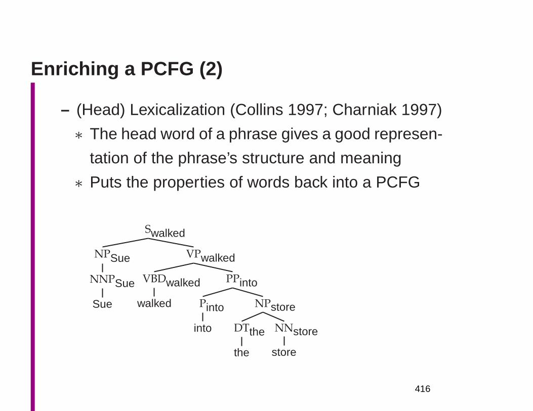
Enriching a PCFG (2)
– (Head) Lexicalization (Collins 1997; Charniak 1997)
∗ The head word of a phrase gives a good represen-
tation of the phrase’s structure and meaning
∗ Puts the properties of words back into a PCFG
Swalked
NPSue
NNPSue
Sue
VPwalked
VBDwalked
walked
PPinto
Pinto
into
NPstore
DTthe
the
NNstore
store
416
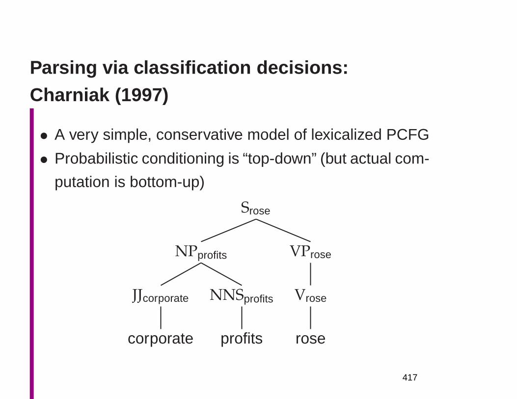
Parsing via classification decisions:Charniak (1997)
• A very simple, conservative model of lexicalized PCFG
• Probabilistic conditioning is “top-down” (but actual com-
putation is bottom-up)
Srose
NPprofits
JJcorporate
corporate
NNSprofits
profits
VProse
Vrose
rose
417
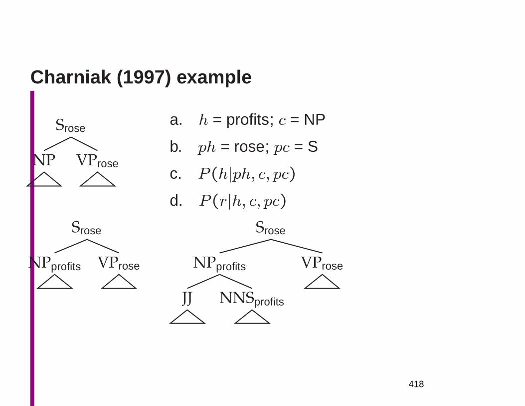
Charniak (1997) example
Srose
NP VProse
a. h = profits; c = NP
b. ph = rose; pc = S
c. P (h|ph, c, pc)d. P (r|h, c, pc)
Srose
NPprofits VProse
Srose
NPprofits
JJ NNSprofits
VProse
418
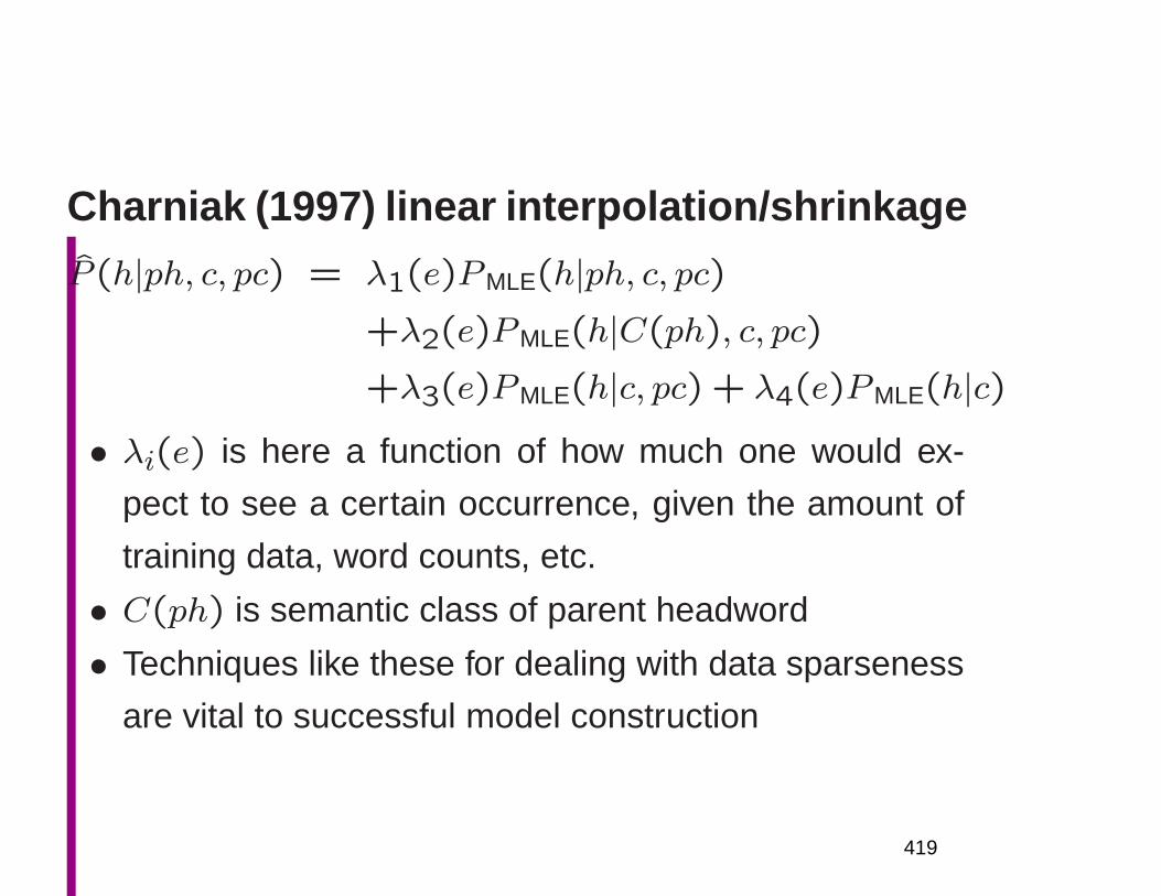
Charniak (1997) linear interpolation/shrinkage
P (h|ph, c, pc) = λ1(e)PMLE(h|ph, c, pc)+λ2(e)PMLE(h|C(ph), c, pc)
+λ3(e)PMLE(h|c, pc) + λ4(e)PMLE(h|c)• λi(e) is here a function of how much one would ex-
pect to see a certain occurrence, given the amount of
training data, word counts, etc.
• C(ph) is semantic class of parent headword
• Techniques like these for dealing with data sparseness
are vital to successful model construction
419
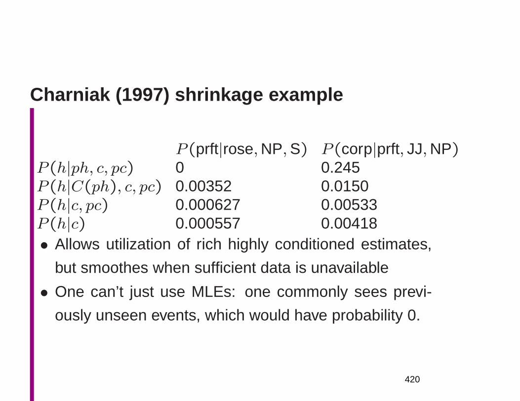
Charniak (1997) shrinkage example
P (prft|rose,NP,S) P (corp|prft, JJ,NP)P (h|ph, c, pc) 0 0.245P (h|C(ph), c, pc) 0.00352 0.0150P (h|c, pc) 0.000627 0.00533P (h|c) 0.000557 0.00418• Allows utilization of rich highly conditioned estimates,
but smoothes when sufficient data is unavailable
• One can’t just use MLEs: one commonly sees previ-
ously unseen events, which would have probability 0.
420
Sparseness & the Penn Treebank
• The Penn Treebank – 1 million words of parsed En-
glish WSJ – has been a key resource (because of the
widespread reliance on supervised learning)
• But 1 million words is like nothing:
– 965,000 constituents, but only 66 WHADJP, of which
only 6 aren’t how much or how many, but there is an
infinite space of these (how clever/original/incompetent
(at risk assessment and evaluation))
• Most of the probabilities that you would like to compute,
you can’t compute
421
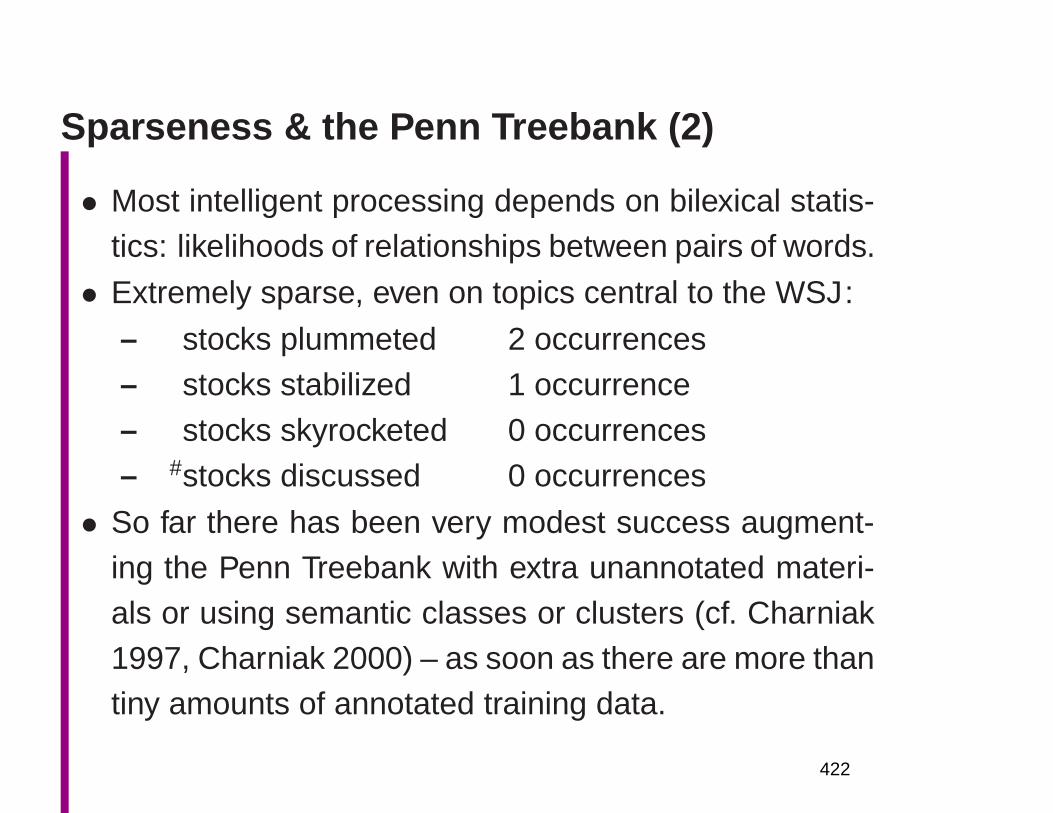
Sparseness & the Penn Treebank (2)
• Most intelligent processing depends on bilexical statis-tics: likelihoods of relationships between pairs of words.
• Extremely sparse, even on topics central to the WSJ:
– stocks plummeted 2 occurrences– stocks stabilized 1 occurrence– stocks skyrocketed 0 occurrences– #stocks discussed 0 occurrences
• So far there has been very modest success augment-ing the Penn Treebank with extra unannotated materi-als or using semantic classes or clusters (cf. Charniak1997, Charniak 2000) – as soon as there are more thantiny amounts of annotated training data.
422
Probabilistic parsing
• Charniak (1997) expands each phrase structure tree in
a single step.
• This is good for capturing dependencies between child
nodes
• But it is bad because of data sparseness
• A pure dependency, one child at a time, model is worse
• But one can do better by in between models, such as
generating the children as a Markov process on both
sides of the head (Collins 1997; Charniak 2000)
423
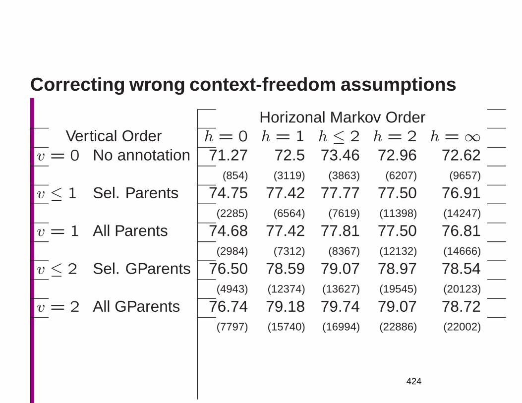
Correcting wrong context-freedom assumptions
Horizonal Markov OrderVertical Order h = 0 h = 1 h ≤ 2 h = 2 h =∞
v = 0 No annotation 71.27 72.5 73.46 72.96 72.62(854) (3119) (3863) (6207) (9657)
v ≤ 1 Sel. Parents 74.75 77.42 77.77 77.50 76.91(2285) (6564) (7619) (11398) (14247)
v = 1 All Parents 74.68 77.42 77.81 77.50 76.81(2984) (7312) (8367) (12132) (14666)
v ≤ 2 Sel. GParents 76.50 78.59 79.07 78.97 78.54(4943) (12374) (13627) (19545) (20123)
v = 2 All GParents 76.74 79.18 79.74 79.07 78.72(7797) (15740) (16994) (22886) (22002)
424
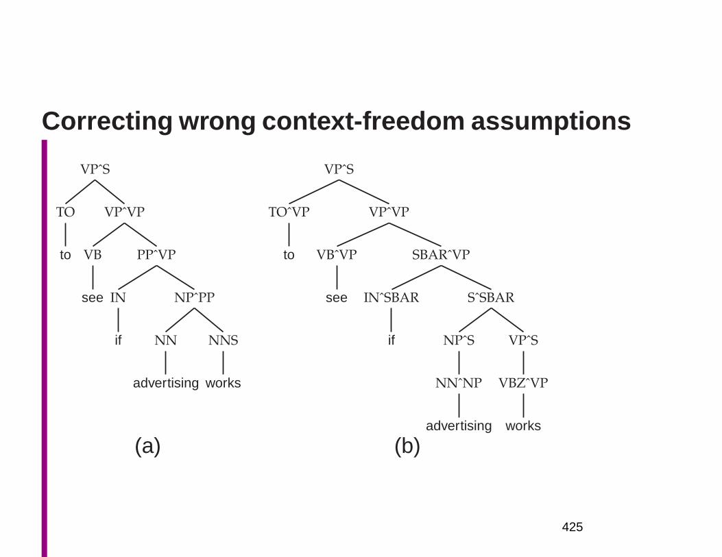
Correcting wrong context-freedom assumptions
VPˆS
TO
to
VPˆVP
VB
see
PPˆVP
IN
if
NPˆPP
NN
advertising
NNS
works
VPˆS
TOˆVP
to
VPˆVP
VBˆVP
see
SBARˆVP
INˆSBAR
if
SˆSBAR
NPˆS
NNˆNP
advertising
VPˆS
VBZˆVP
works
(a) (b)
425
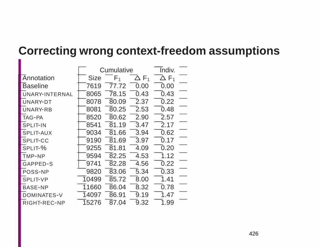
Correcting wrong context-freedom assumptions
Cumulative Indiv.Annotation Size F1 ∆ F1 ∆ F1
Baseline 7619 77.72 0.00 0.00UNARY-INTERNAL 8065 78.15 0.43 0.43UNARY-DT 8078 80.09 2.37 0.22UNARY-RB 8081 80.25 2.53 0.48TAG-PA 8520 80.62 2.90 2.57SPLIT-IN 8541 81.19 3.47 2.17SPLIT-AUX 9034 81.66 3.94 0.62SPLIT-CC 9190 81.69 3.97 0.17SPLIT-% 9255 81.81 4.09 0.20TMP-NP 9594 82.25 4.53 1.12GAPPED-S 9741 82.28 4.56 0.22POSS-NP 9820 83.06 5.34 0.33SPLIT-VP 10499 85.72 8.00 1.41BASE-NP 11660 86.04 8.32 0.78DOMINATES-V 14097 86.91 9.19 1.47RIGHT-REC-NP 15276 87.04 9.32 1.99
426
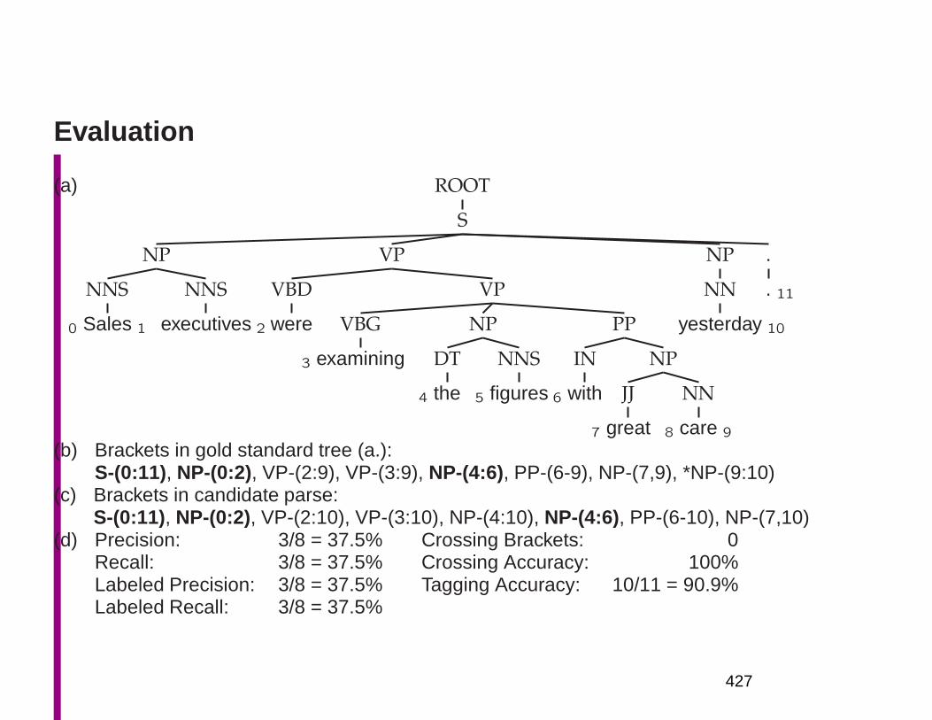
Evaluation
(a) ROOT
S
NP
NNS
0 Sales 1
NNS
executives 2
VP
VBD
were
VP
VBG
3 examining
NP
DT
4 the
NNS
5 figures
PP
IN
6 with
NP
JJ
7 great
NN
8 care 9
NP
NN
yesterday 10
.
. 11
(b) Brackets in gold standard tree (a.):S-(0:11), NP-(0:2), VP-(2:9), VP-(3:9), NP-(4:6), PP-(6-9), NP-(7,9), *NP-(9:10)
(c) Brackets in candidate parse:S-(0:11), NP-(0:2), VP-(2:10), VP-(3:10), NP-(4:10), NP-(4:6), PP-(6-10), NP-(7,10)
(d) Precision: 3/8 = 37.5% Crossing Brackets: 0Recall: 3/8 = 37.5% Crossing Accuracy: 100%Labeled Precision: 3/8 = 37.5% Tagging Accuracy: 10/11 = 90.9%Labeled Recall: 3/8 = 37.5%
427
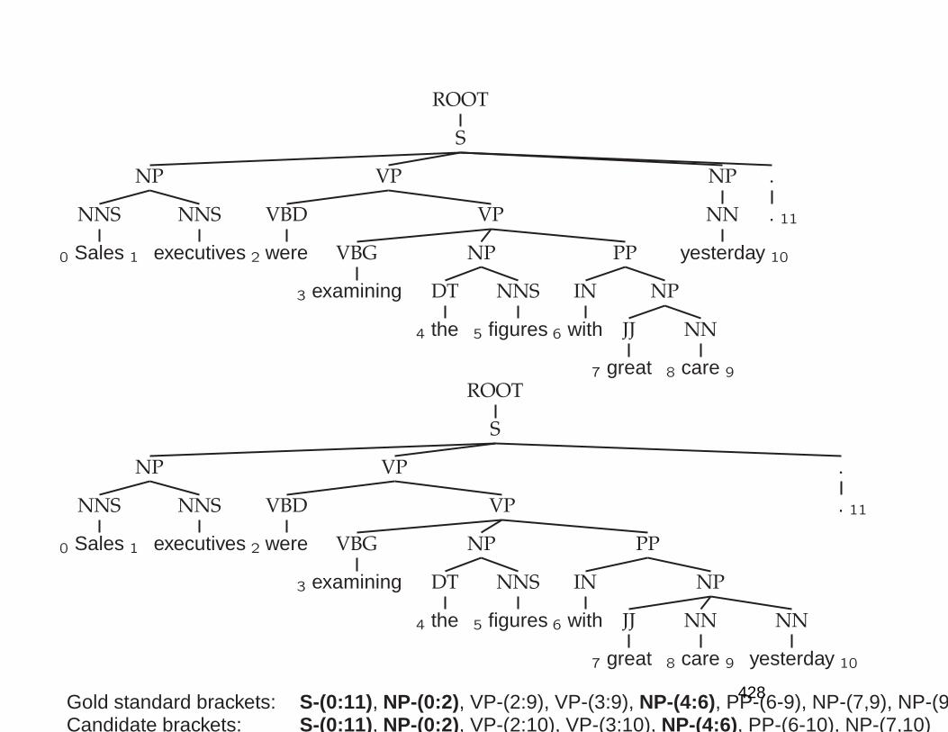
ROOT
S
NP
NNS
0 Sales 1
NNS
executives 2
VP
VBD
were
VP
VBG
3 examining
NP
DT
4 the
NNS
5 figures
PP
IN
6 with
NP
JJ
7 great
NN
8 care 9
NP
NN
yesterday 10
.
. 11
ROOT
S
NP
NNS
0 Sales 1
NNS
executives 2
VP
VBD
were
VP
VBG
3 examining
NP
DT
4 the
NNS
5 figures
PP
IN
6 with
NP
JJ
7 great
NN
8 care 9
NN
yesterday 10
.
. 11
Gold standard brackets: S-(0:11), NP-(0:2), VP-(2:9), VP-(3:9), NP-(4:6), PP-(6-9), NP-(7,9), NP-(9:10)Candidate brackets: S-(0:11), NP-(0:2), VP-(2:10), VP-(3:10), NP-(4:6), PP-(6-10), NP-(7,10)
428

1

Gold standard brackets: S-(0:11), NP-(0:2), VP-(2:9), VP-(3:9), NP-(4:6), PP-(6-9), NP-(7,9), NP-(9:10)
Candidate brackets: S-(0:11), NP-(0:2), VP-(2:10), VP-(3:10), NP-(4:6), PP-(6-10), NP-(7,10)
Labeled Precision: 3/7 = 42.9%Labeled Recall: 3/8 = 37.5%LP/LR F1 40.0%Tagging Accuracy: 11/11 = 100.0%
429
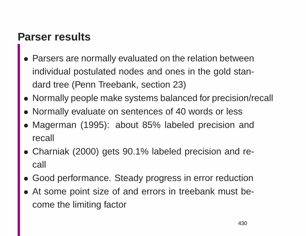
Parser results
• Parsers are normally evaluated on the relation betweenindividual postulated nodes and ones in the gold stan-dard tree (Penn Treebank, section 23)
• Normally people make systems balanced for precision/recall
• Normally evaluate on sentences of 40 words or less
• Magerman (1995): about 85% labeled precision andrecall
• Charniak (2000) gets 90.1% labeled precision and re-call
• Good performance. Steady progress in error reduction
• At some point size of and errors in treebank must be-come the limiting factor
430

1
– (Some thought that was in 1997, when several sys-
tems were getting 87.x%, but apparently not.)
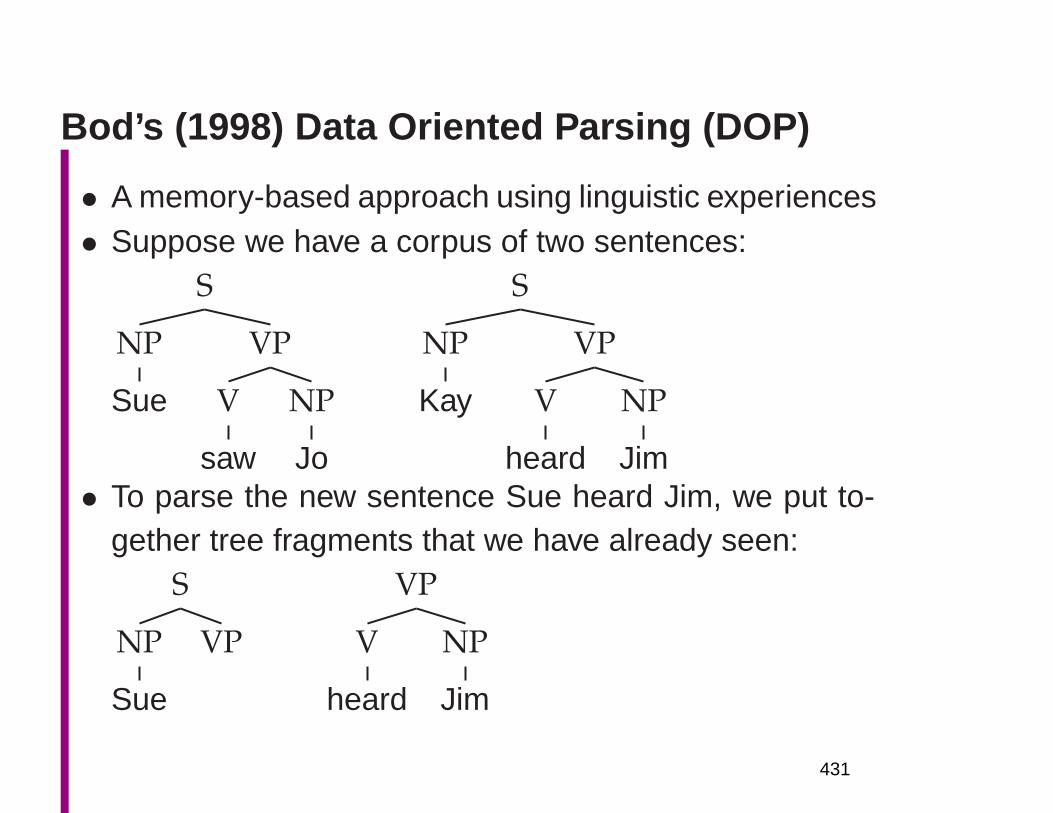
Bod’s (1998) Data Oriented Parsing (DOP)
• A memory-based approach using linguistic experiences• Suppose we have a corpus of two sentences:
S
NP
Sue
VP
V
saw
NP
Jo
S
NP
Kay
VP
V
heard
NP
Jim• To parse the new sentence Sue heard Jim, we put to-
gether tree fragments that we have already seen:S
NP
Sue
VP
VP
V
heard
NP
Jim
431
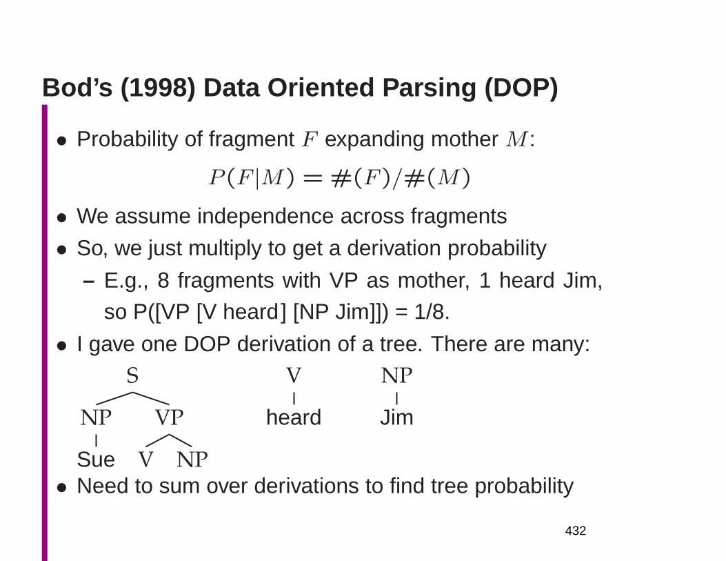
Bod’s (1998) Data Oriented Parsing (DOP)
• Probability of fragment F expanding mother M :
P (F |M) = #(F)/#(M)
• We assume independence across fragments
• So, we just multiply to get a derivation probability
– E.g., 8 fragments with VP as mother, 1 heard Jim,so P([VP [V heard ] [NP Jim]]) = 1/8.
• I gave one DOP derivation of a tree. There are many:S
NP
Sue
VP
V NP
V
heard
NP
Jim
• Need to sum over derivations to find tree probability
432
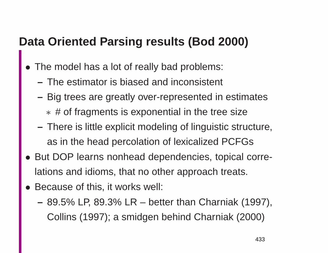
Data Oriented Parsing results (Bod 2000)
• The model has a lot of really bad problems:
– The estimator is biased and inconsistent
– Big trees are greatly over-represented in estimates
∗ # of fragments is exponential in the tree size
– There is little explicit modeling of linguistic structure,
as in the head percolation of lexicalized PCFGs
• But DOP learns nonhead dependencies, topical corre-
lations and idioms, that no other approach treats.
• Because of this, it works well:
– 89.5% LP, 89.3% LR – better than Charniak (1997),
Collins (1997); a smidgen behind Charniak (2000)
433

Extra/variant slides
434

Statistical Parsing
• Recent work on statistical parsing, including (Mager-man 1995; Charniak 1997; Collins 1996, 1997; Ratna-parkhi 1997b; Charniak 2000) has greatly raised thebar of parsing performance
• It’s redefined the ability to do robust, rapid broad cover-age parsing
– Around 1990: Probably no parser could do betterthan around 65% labeled precision/recall over broadcoverage text (evaluation was less rigorous)
– 2000: Over 90% labeled precision/recall
• How? By converting parsing into a classification taskand using machine learning methods
435
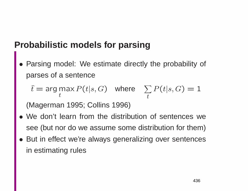
Probabilistic models for parsing
• Parsing model: We estimate directly the probability of
parses of a sentence
t = argmaxt
P (t|s,G) where∑
tP (t|s,G) = 1
(Magerman 1995; Collins 1996)
• We don’t learn from the distribution of sentences we
see (but nor do we assume some distribution for them)
• But in effect we’re always generalizing over sentences
in estimating rules
436
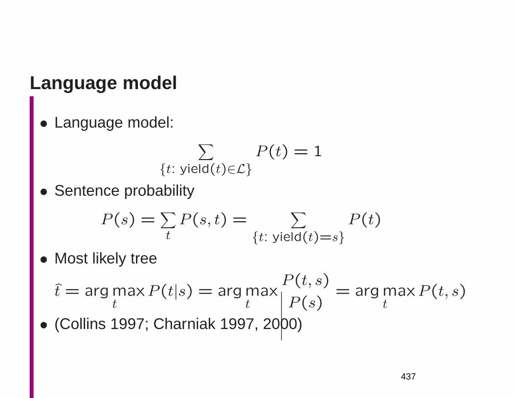
Language model
• Language model:∑
t: yield(t)∈LP (t) = 1
• Sentence probability
P (s) =∑
tP (s, t) =
∑
t: yield(t)=sP (t)
• Most likely tree
t = argmaxt
P (t|s) = argmaxt
P (t, s)
P (s)= argmax
tP (t, s)
• (Collins 1997; Charniak 1997, 2000)
437
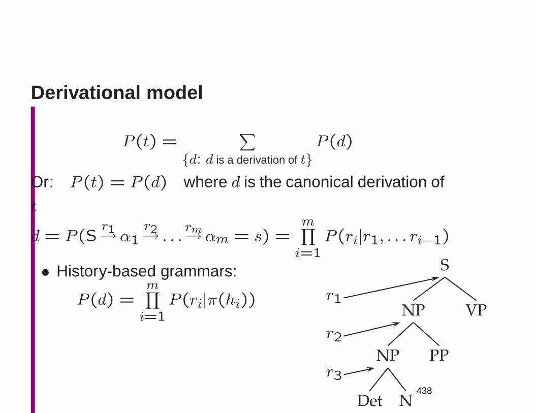
Derivational model
P (t) =∑
d: d is a derivation of tP (d)
Or: P (t) = P (d) where d is the canonical derivation of
t
d = P (Sr1→α1
r2→ . . .rm→αm = s) =
m∏
i=1P (ri|r1, . . . ri−1)
• History-based grammars:
P (d) =m∏
i=1P (ri|π(hi)) r1
r2
r3
S
NP
NP
Det N
PP
VP
438
Enrichments
• Structure sensitivity
– Expansions of nodes depends a lot on their position
in the tree (independent of lexical content)
– (Manning and Carpenter 1997; Johnson 1998a)
• Lexicalization – getting back properties of words
439
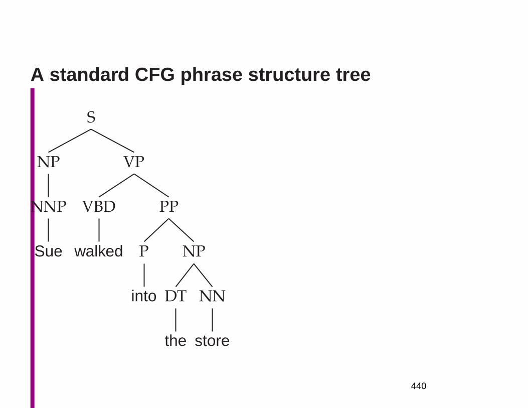
A standard CFG phrase structure tree
S
NP
NNP
Sue
VP
VBD
walked
PP
P
into
NP
DT
the
NN
store
440
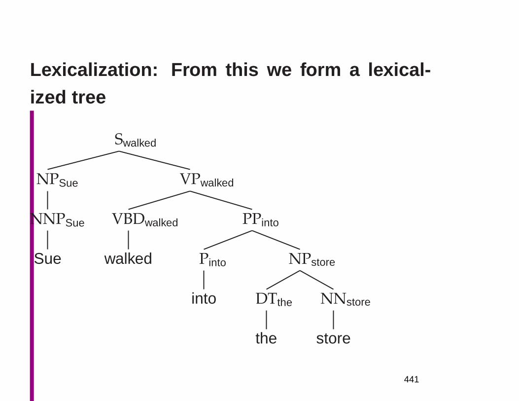
Lexicalization: From this we form a lexical-ized tree
Swalked
NPSue
NNPSue
Sue
VPwalked
VBDwalked
walked
PPinto
Pinto
into
NPstore
DTthe
the
NNstore
store
441
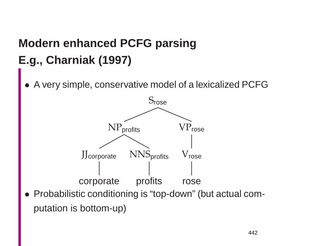
Modern enhanced PCFG parsingE.g., Charniak (1997)
• A very simple, conservative model of a lexicalized PCFG
Srose
NPprofits
JJcorporate
corporate
NNSprofits
profits
VProse
Vrose
rose• Probabilistic conditioning is “top-down” (but actual com-
putation is bottom-up)
442

Charniak (1997) example
Srose
NP VProse
a. h = profits; c = NP
b. ph = rose; pc = S
c. P (h|ph, c, pc)d. P (r|h, c, pc)
Srose
NPprofits VProse
Srose
NPprofits
JJ NNSprofits
VProse
443

Charniak (1997) linear interpolation/shrinkage
P (h|ph, c, pc) = λ1(e)PMLE(h|ph, c, pc)+λ2(e)PMLE(h|C(ph), c, pc)
+λ3(e)PMLE(h|c, pc) + λ4(e)PMLE(h|c)• λi(e) is here a function of how much one would ex-
pect to see a certain occurrence, given the amount of
training data, word counts, etc.
• C(ph) is semantic class of parent headword
• Techniques like these for dealing with data sparseness
are vital to successful model construction
444
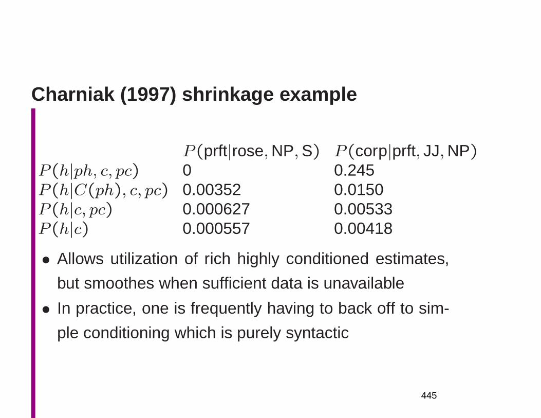
Charniak (1997) shrinkage example
P (prft|rose,NP,S) P (corp|prft, JJ,NP)P (h|ph, c, pc) 0 0.245P (h|C(ph), c, pc) 0.00352 0.0150P (h|c, pc) 0.000627 0.00533P (h|c) 0.000557 0.00418
• Allows utilization of rich highly conditioned estimates,
but smoothes when sufficient data is unavailable
• In practice, one is frequently having to back off to sim-
ple conditioning which is purely syntactic
445
Topics in InformationRetrieval
FSNLP, chapter 15
Christopher Manning andHinrich Schütze
© 1999–2001446
Information Retrieval
• Getting information from document repositories
• Normally text (though spoken, image, and video data
are all becoming more important)
• Traditionally a rather separate field from NLP, and al-
ways very empirically based
• A field of some antiquity: the famous SMART IR system
(Salton) predates the relational model in databases
• New directions: the Web, email, multimedia, . . .
• There is much scope for greater profitable interaction
between IR and Statistical NLP
447
Tasks
• “Ad hoc retrieval”: the user enters query terms which
describe the desired information; the system returns a
set of (sometimes ranked) documents.
• Document categorization: assign a document to one or
more categories (e.g., subject codes) [chapter 16]
– Filtering: categorization with binary choice about the
relevance of a document (e.g., screen for junk email).
– Routing: categorization for the purpose of transmit-
ting a document to one or more users (e.g., cus-
tomer service by product)
448
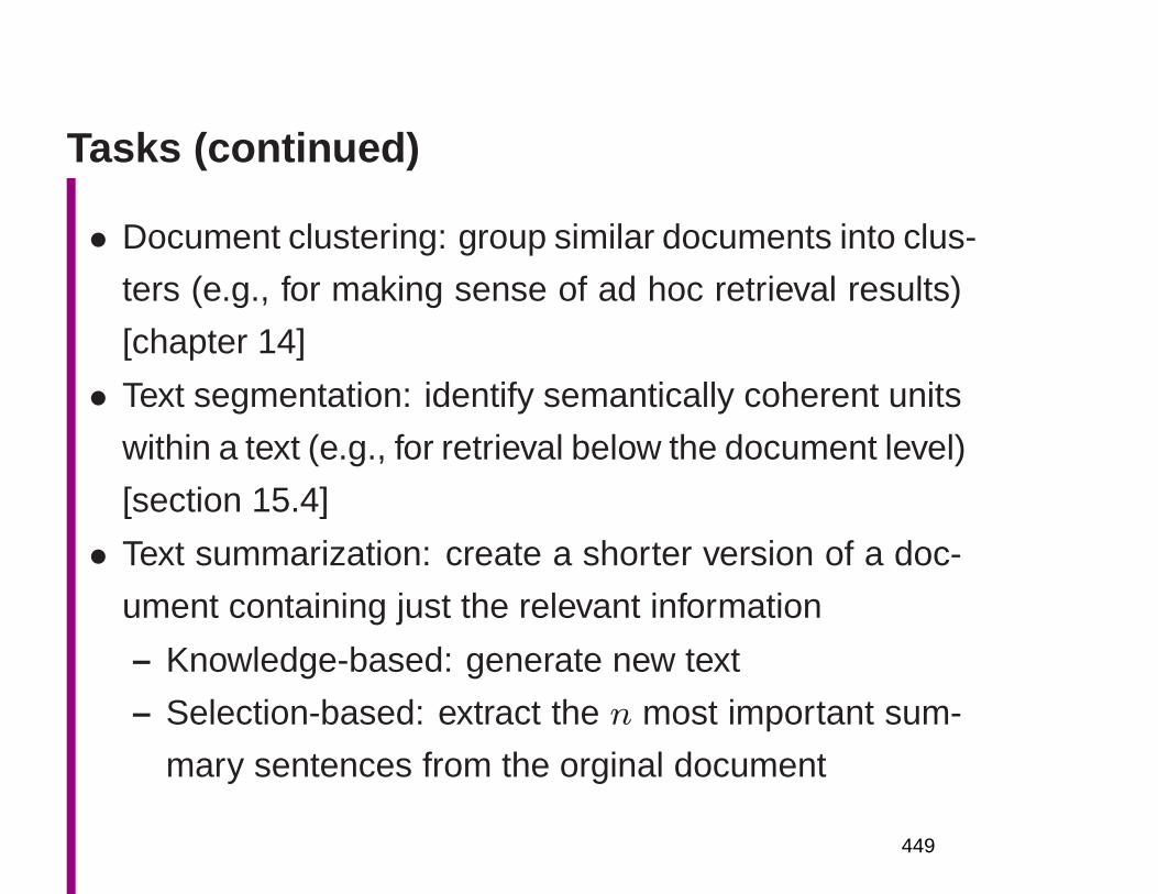
Tasks (continued)
• Document clustering: group similar documents into clus-
ters (e.g., for making sense of ad hoc retrieval results)
[chapter 14]
• Text segmentation: identify semantically coherent units
within a text (e.g., for retrieval below the document level)
[section 15.4]
• Text summarization: create a shorter version of a doc-
ument containing just the relevant information
– Knowledge-based: generate new text
– Selection-based: extract the n most important sum-
mary sentences from the orginal document
449

[ AltaVista] [ Advanced Query] [ Simple Query] [ Private eXtension Products] [ Help with Query]
Search the Web UsenetDisplay results Compact Detailed
Tip: When in doubt use lower-case. Check out Help for better matches.
Word count: glass pyramid: about 200; Pei:9453; Louvre:26578
Documents 1-10 of about 10000 matching the query, best matches first.
Paris, FranceParis, France. Practical Info.-A Brief Overview. Layout: One of the most densely populated citiesin Europe, Paris is also one of the most accessible,...http://www.catatravel.com/paris.htm - size 8K - 29 Sep 95
CultureCulture. French culture is an integral part of France’s image, as foreign tourists are the first toacknowledge by thronging to the Louvre and the Centre..http://www.france.diplomatie.fr/france/edu/culture.gb.html - size 48K - 20 Jun 96
Travel World - Science Education Tour of EuropeScience Education Tour of Europe. B E M I D J I S T A T E U N I V E R S I T Y ScienceEducation Tour of EUROPE July 19-August 1, 1995...http://www.omnitravel.com/007etour.html - size 16K - 21 Jul 95http://www.omnitravel.com/etour.html - size 16K - 15 May 95
FRANCE REAL ESTATE RENTALLOIRE VALLEY RENTAL. ANCIENT STONE HOME FOR RENT. Available to rent is afurnished, french country decorated, two bedroom, small stone home, built in the..http://frost2.flemingc.on.ca/~pbell/france.htm - size 10K - 21 Jun 96
LINKSPAUL’S LINKS. Click here to view CNN interactive and WEBNEWSor CNET. Click here tomake your own web site. Click here to manage your cash. Interested in...http://frost2.flemingc.on.ca/~pbell/links.htm - size 9K - 19 Jun 96
Digital Design Media, Chapter 9: Lines in SpaceConstruction planes... Glass-sheet models... Three-dimensional geometric transformations...Sweeping points... Space curves... Structuring wireframe...http://www.gsd.harvard.edu/~malcolm/DDM/DDM09.html - size 36K - 22 Jul 95
No TitleBoston Update 94: A VISION FOR BOSTON’S FUTURE. Ian Menzies. Senior Fellow,McCormack Institute. University of Massachusetts Boston. April 1994. Prepared..http://www.cs.umb.edu/~serl/mcCormack/Menzies.html - size 25K - 31 Jan 96
Paris - PhotographThe Arc de Triomphe du Carrousel neatly frames IM Pei’s glass pyramid, Paris 1/6. © 1996Richard Nebesky.
Results of the search ‘ “glass pyramid” Pei Louvre’ on AltaVista
450
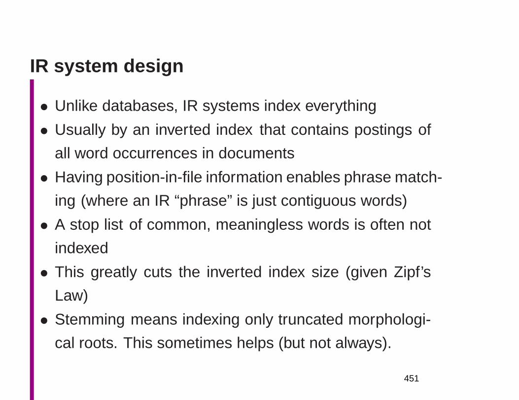
IR system design
• Unlike databases, IR systems index everything
• Usually by an inverted index that contains postings of
all word occurrences in documents
• Having position-in-file information enables phrase match-
ing (where an IR “phrase” is just contiguous words)
• A stop list of common, meaningless words is often not
indexed
• This greatly cuts the inverted index size (given Zipf’s
Law)
• Stemming means indexing only truncated morphologi-
cal roots. This sometimes helps (but not always).
451
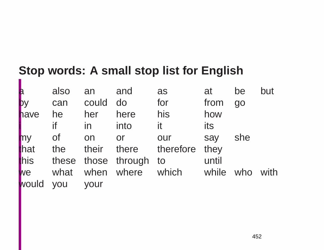
Stop words: A small stop list for English
a also an and as at be butby can could do for from gohave he her here his howi if in into it itsmy of on or our say shethat the their there therefore theythis these those through to untilwe what when where which while who withwould you your
452

The probability ranking principle (PRP)
IR fundamentally addresses this problem: Given a query
W1 and a document W2 attempt to decide relevance of
W2 to W1, where relevance is meant to be computed with
respect to their hidden meanings M1 and M2.
The model underlying most IR systems (van Rijsbergen
1979: 113):
• PRP: Rank documents in order of decreasing probabil-
ity of relevance is optimal.
Problems: documents that aren’t independent. Any that
don’t give additional information (especially, duplicates!).
Implies not doing word-sense disambiguation.
453
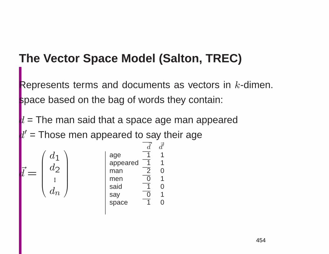
The Vector Space Model (Salton, TREC)
Represents terms and documents as vectors in k-dimen.
space based on the bag of words they contain:
d = The man said that a space age man appeared
d′ = Those men appeared to say their age
~d =
d1d2...dn
~d ~d′
age 1 1appeared 1 1man 2 0men 0 1said 1 0say 0 1space 1 0
454
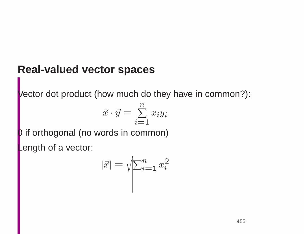
Real-valued vector spaces
Vector dot product (how much do they have in common?):
~x · ~y =n
∑
i=1xiyi
0 if orthogonal (no words in common)
Length of a vector:
|~x| =√
∑ni=1 x
2i
455
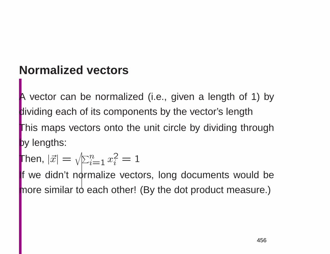
Normalized vectors
A vector can be normalized (i.e., given a length of 1) by
dividing each of its components by the vector’s length
This maps vectors onto the unit circle by dividing through
by lengths:
Then, |~x| =√
∑ni=1 x
2i = 1
If we didn’t normalize vectors, long documents would be
more similar to each other! (By the dot product measure.)
456
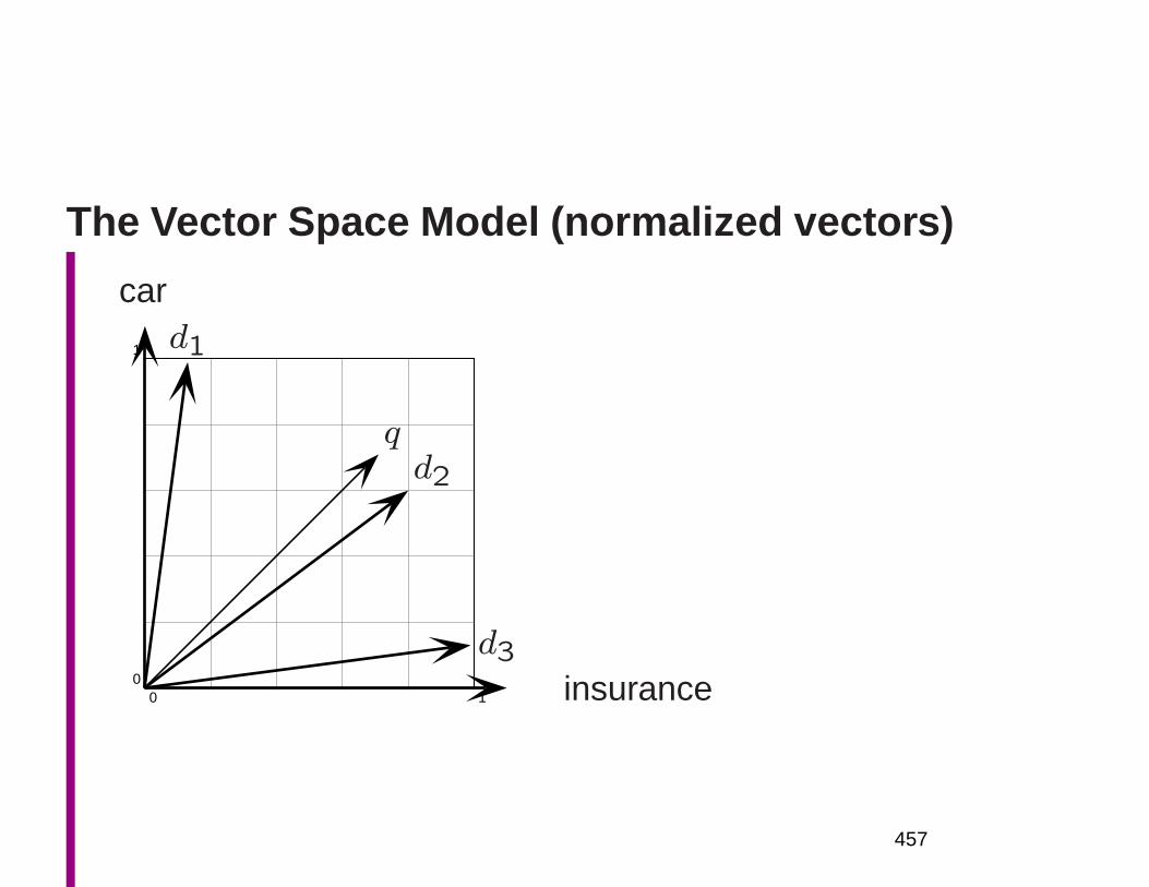
The Vector Space Model (normalized vectors)
0 10
1
insurance
car
q
d1
d2
d3
457
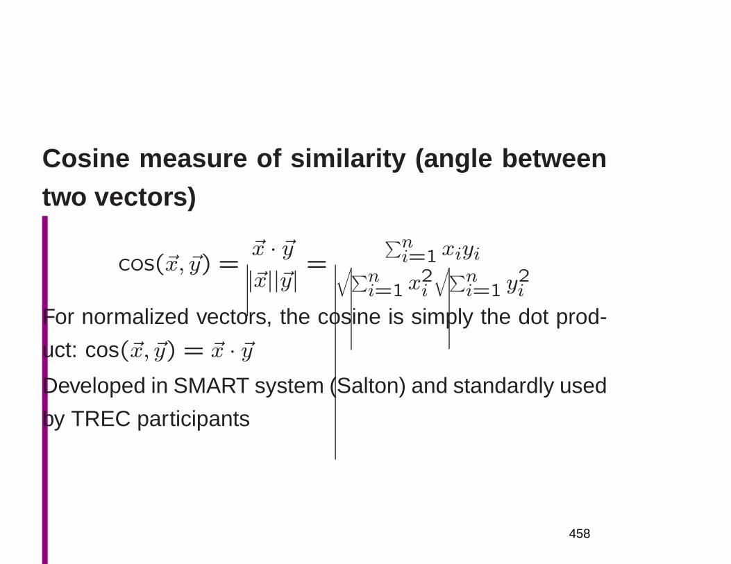
Cosine measure of similarity (angle betweentwo vectors)
cos(~x, ~y) =~x · ~y|~x||~y| =
∑ni=1 xiyi
√
∑ni=1 x
2i
√
∑ni=1 y
2i
For normalized vectors, the cosine is simply the dot prod-
uct: cos(~x, ~y) = ~x · ~yDeveloped in SMART system (Salton) and standardly used
by TREC participants
458
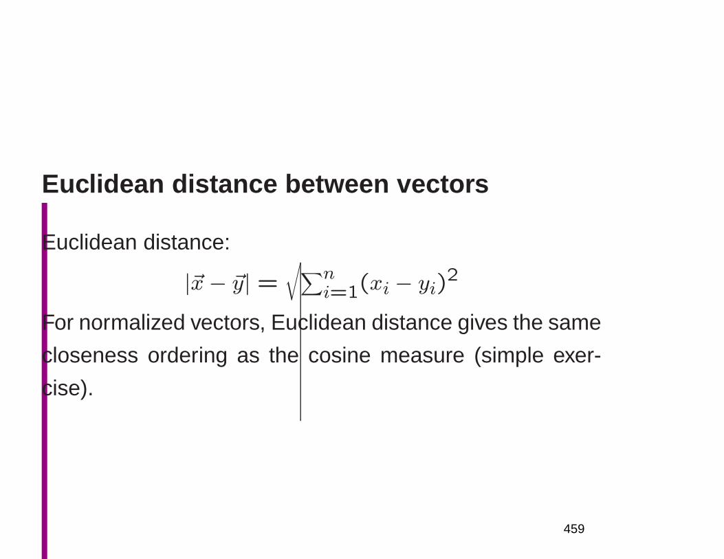
Euclidean distance between vectors
Euclidean distance:
|~x− ~y| =√
∑ni=1(xi − yi)
2
For normalized vectors, Euclidean distance gives the same
closeness ordering as the cosine measure (simple exer-
cise).
459
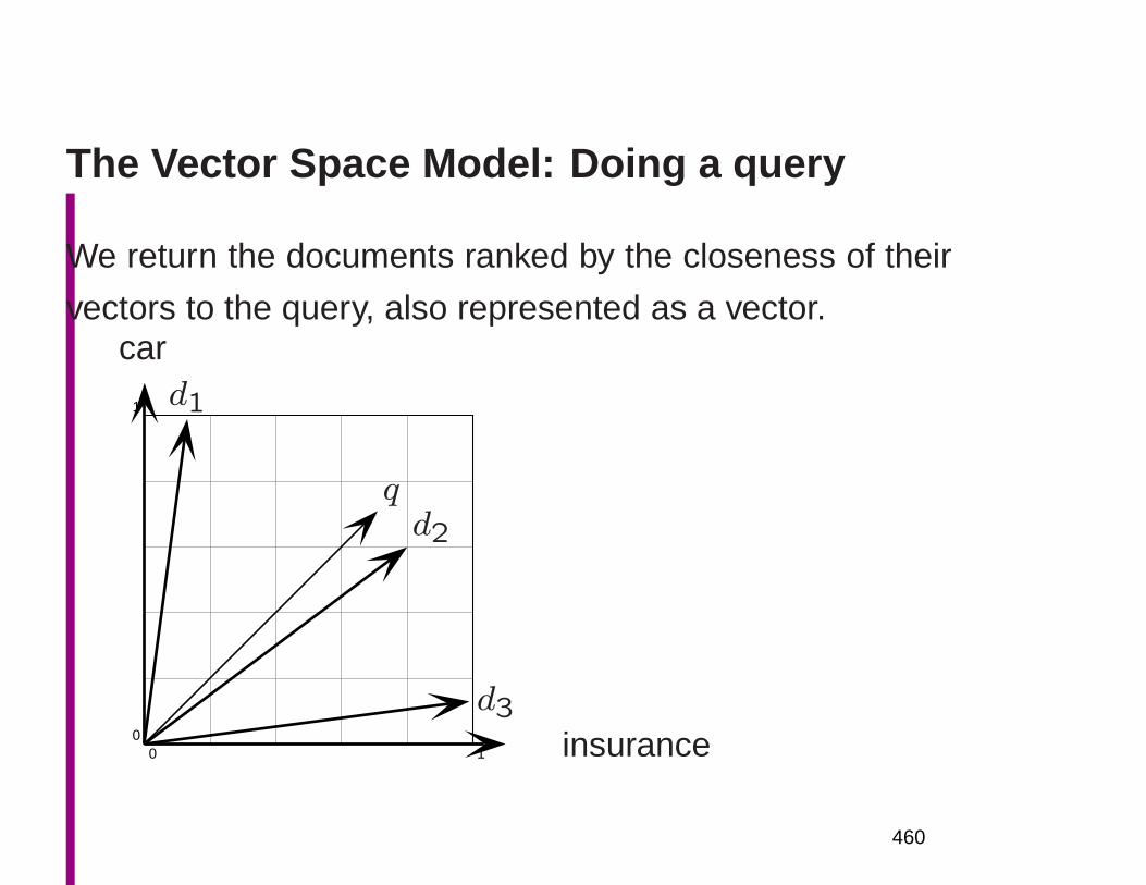
The Vector Space Model: Doing a query
We return the documents ranked by the closeness of their
vectors to the query, also represented as a vector.
0 10
1
insurance
car
q
d1
d2
d3
460
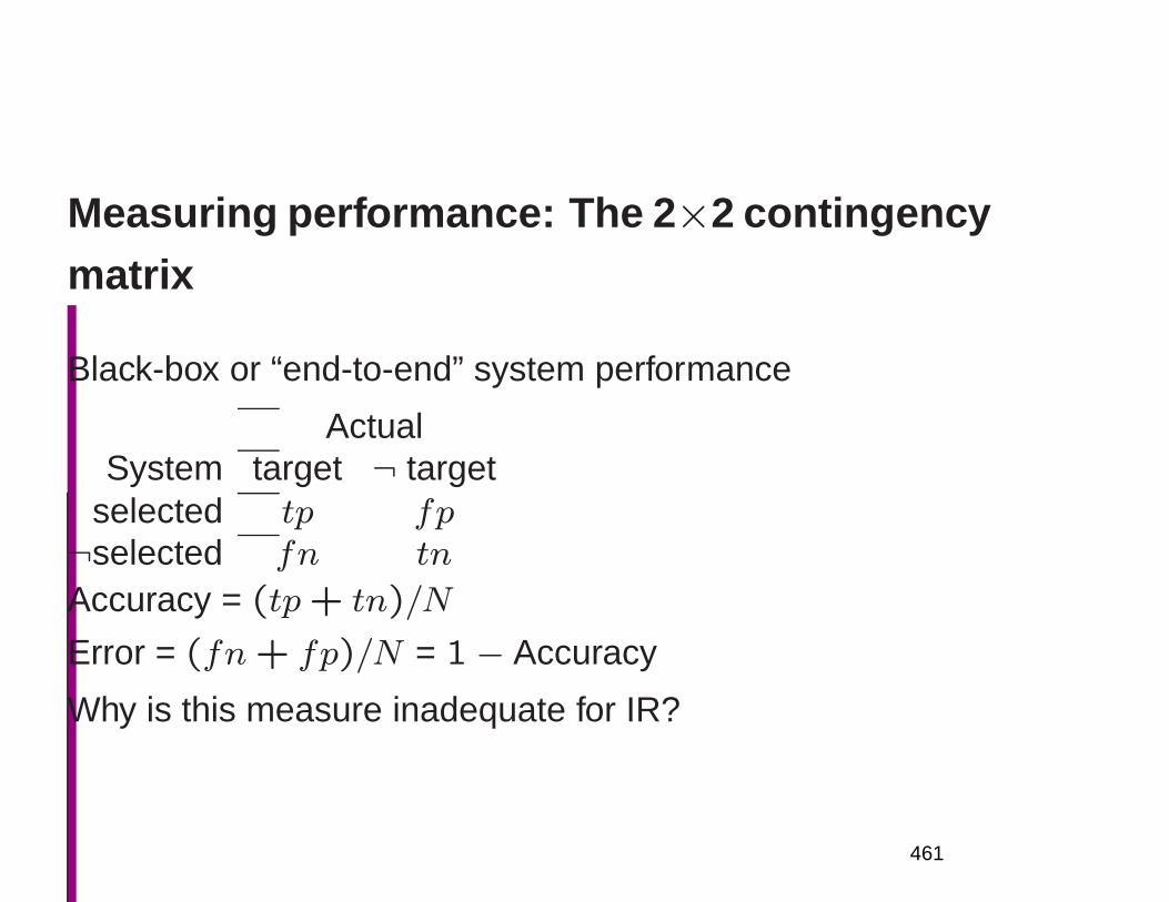
Measuring performance: The 2 ×2 contingencymatrix
Black-box or “end-to-end” system performance
ActualSystem target ¬ target
selected tp fp¬selected fn tn
Accuracy = (tp+ tn)/N
Error = (fn+ fp)/N = 1− Accuracy
Why is this measure inadequate for IR?
461
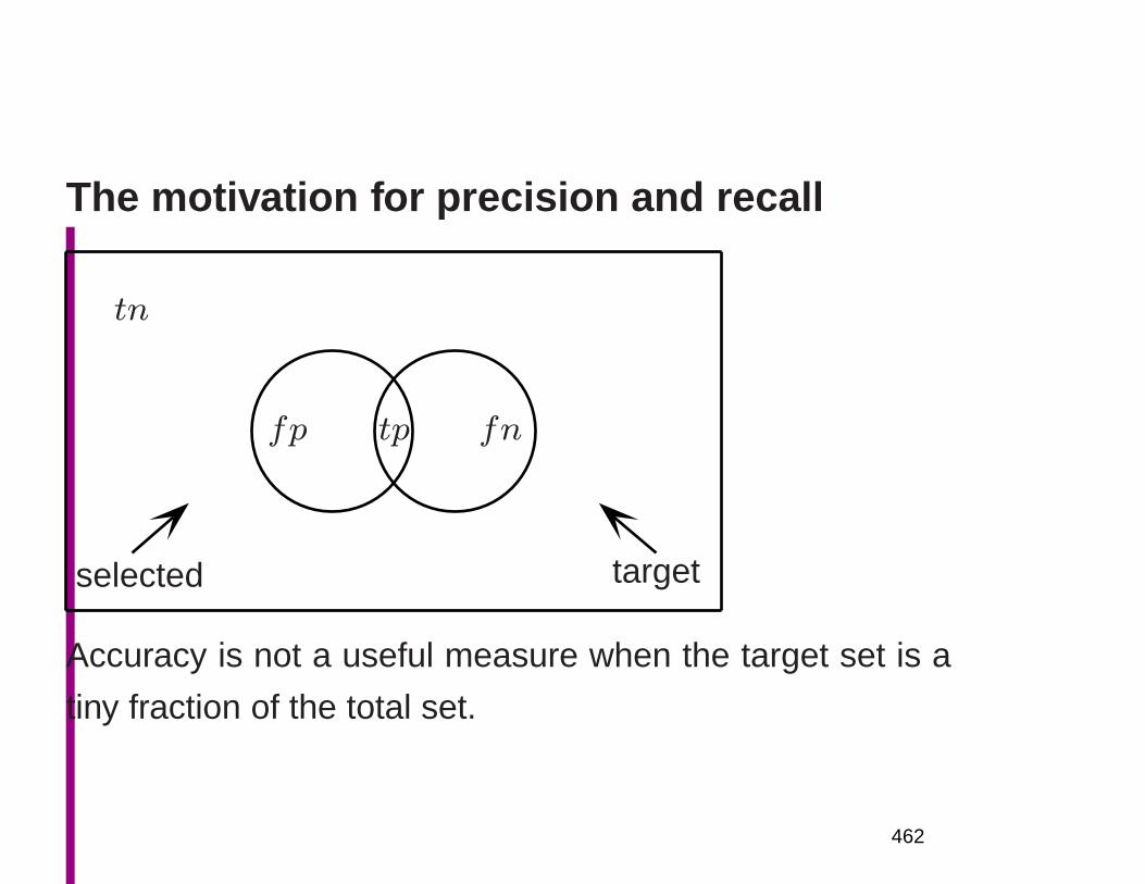
The motivation for precision and recall
tpfp fn
selected target
tn
Accuracy is not a useful measure when the target set is a
tiny fraction of the total set.
462
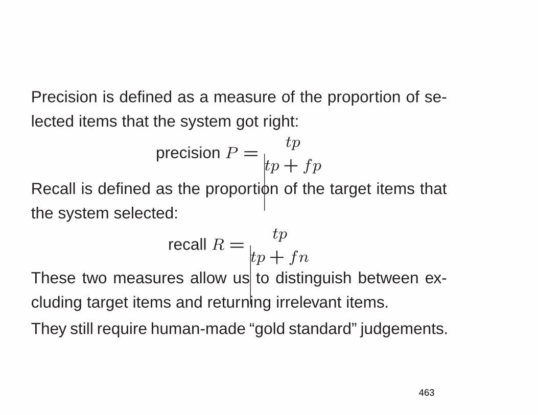
Precision is defined as a measure of the proportion of se-
lected items that the system got right:
precision P =tp
tp+ fp
Recall is defined as the proportion of the target items that
the system selected:
recall R =tp
tp+ fn
These two measures allow us to distinguish between ex-
cluding target items and returning irrelevant items.
They still require human-made “gold standard” judgements.
463
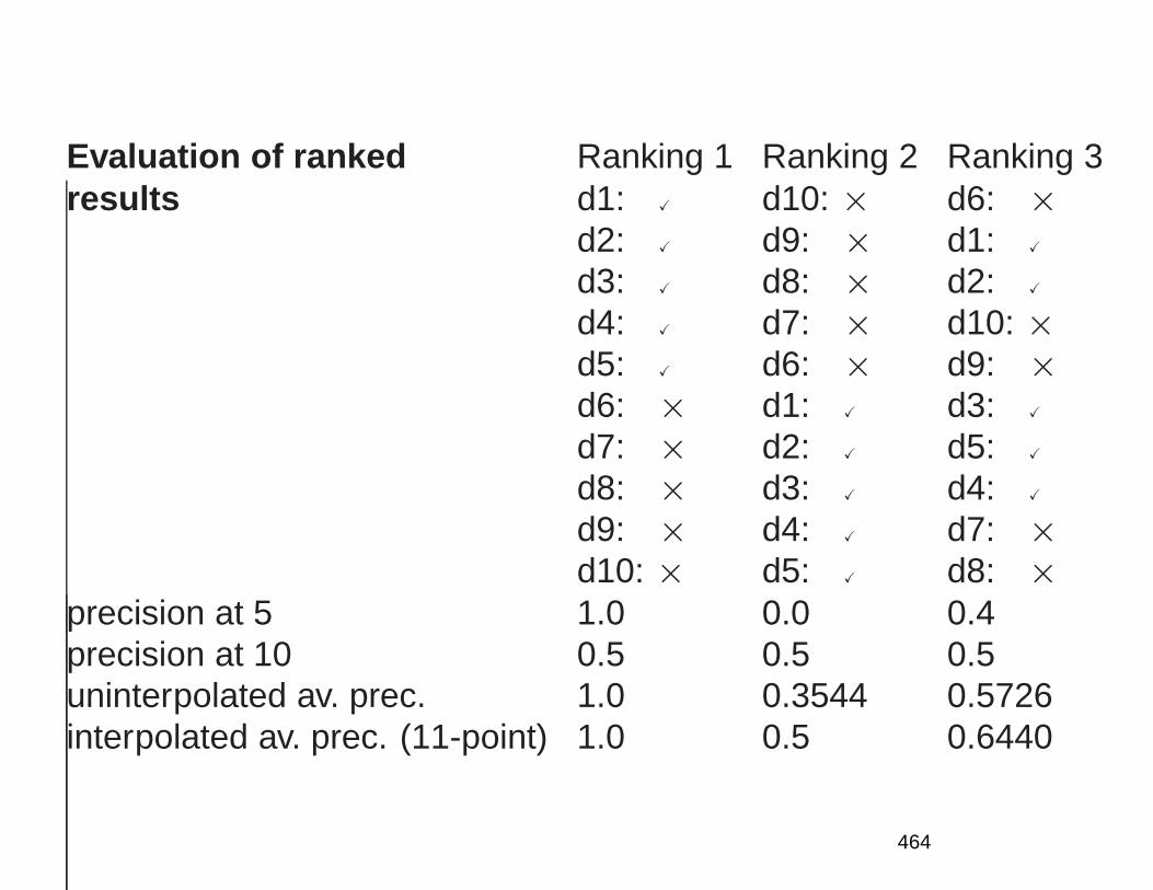
Evaluation of ranked Ranking 1 Ranking 2 Ranking 3results d1: X d10: × d6: ×
d2: X d9: × d1: X
d3: X d8: × d2: X
d4: X d7: × d10: ×d5: X d6: × d9: ×d6: × d1: X d3: X
d7: × d2: X d5: X
d8: × d3: X d4: X
d9: × d4: X d7: ×d10: × d5: X d8: ×
precision at 5 1.0 0.0 0.4precision at 10 0.5 0.5 0.5uninterpolated av. prec. 1.0 0.3544 0.5726interpolated av. prec. (11-point) 1.0 0.5 0.6440
464
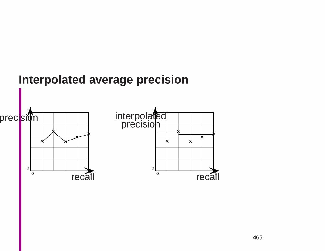
Interpolated average precision
0 10
1
××
×× ×
precision
recall 0 10
1
××
×× ×
interpolatedprecision
recall
465
Combined measures
If we can decide on the relative importance of precision and
recall, then they can be combined into a single measure.
Does one just average them? Bad, because the measures
aren’t independent.
What’s a sensible model?
Rijsbergen (1979:174) defines and justifies the usually used
alternative, the F measure
(see http://www.dcs.gla.ac.uk/Keith/Preface.html).
466

Assumptions:
• Interested in document proportions not absolute num-
bers
• Decreasing marginal effectiveness of recall and preci-
sion, e.g.:
(R+ 1, P − 1) > (R,P )
but
(R+ 1, P ) > (R+ 2, P − 1)
Makes curves convex towards origin.
467
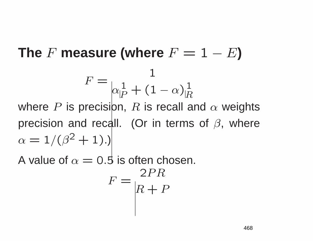
The F measure (where F = 1− E)
F =1
α1P + (1− α)1
R
where P is precision, R is recall and α weights
precision and recall. (Or in terms of β, where
α = 1/(β2 + 1).)
A value of α = 0.5 is often chosen.
F =2PR
R+ P
468
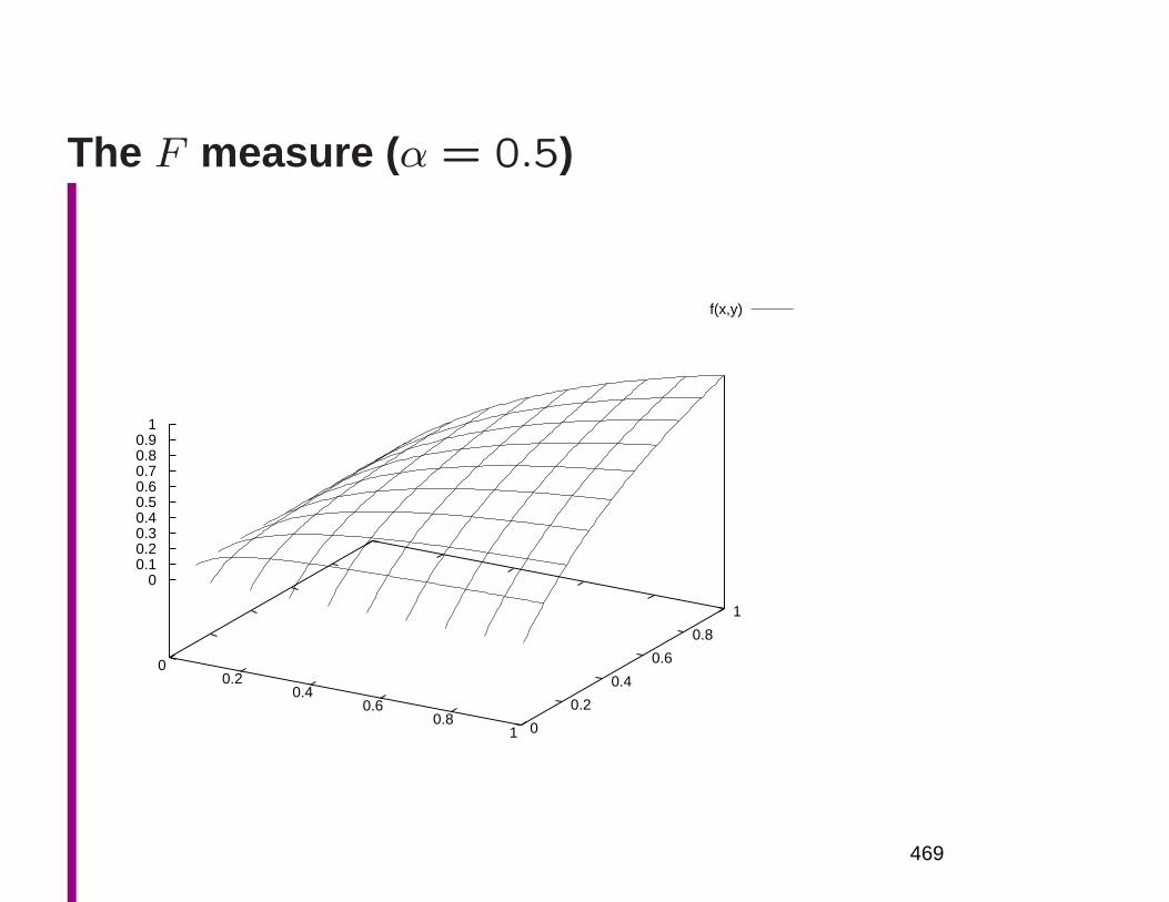
The F measure ( α = 0.5)
f(x,y)
00.2
0.40.6
0.81 0
0.2
0.4
0.6
0.8
1
00.10.20.30.40.50.60.70.80.9
1
469
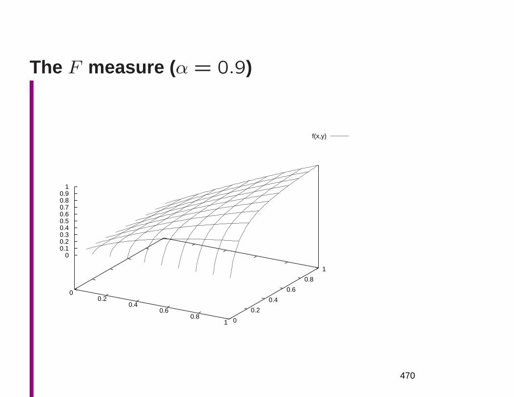
The F measure ( α = 0.9)
f(x,y)
00.2
0.40.6
0.81 0
0.2
0.4
0.6
0.8
1
00.10.20.30.40.50.60.70.80.9
1
470
Term weighting
• Simplest term (vector component) weightings are:
– count of number of times word occurs in document
– binary: word does or doesn’t occur in document
• However, general experience is that a document is a
better match if a word occurs three times than once,
but not a three times better match.
• This leads to a series of weighting functions that dampthe term weighting, e.g., 1 + log(x), x > 0, or
√x.
• This is a good thing to do, but still imperfect: it doesn’t
capture that the occurrence of a term in a document
is more important if that term does not occur in many
other documents.
471
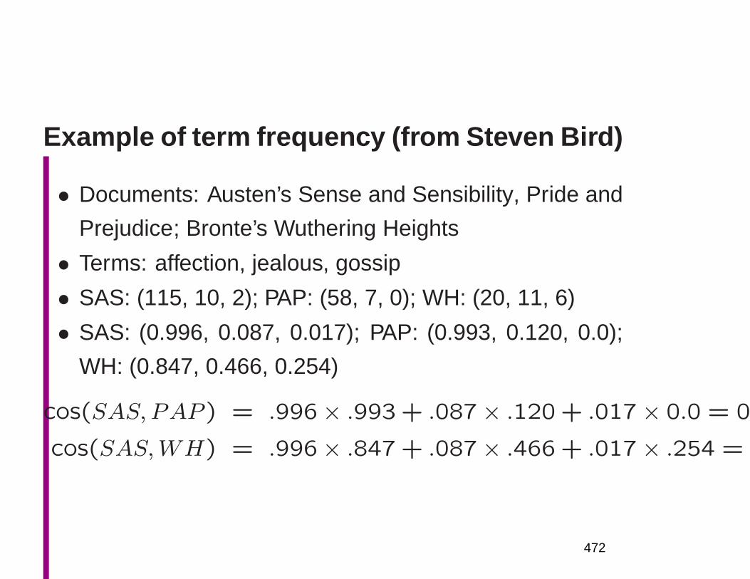
Example of term frequency (from Steven Bird)
• Documents: Austen’s Sense and Sensibility, Pride and
Prejudice; Bronte’s Wuthering Heights
• Terms: affection, jealous, gossip
• SAS: (115, 10, 2); PAP: (58, 7, 0); WH: (20, 11, 6)
• SAS: (0.996, 0.087, 0.017); PAP: (0.993, 0.120, 0.0);
WH: (0.847, 0.466, 0.254)
cos(SAS, PAP ) = .996× .993 + .087× .120 + .017× 0.0 = 0.
cos(SAS,WH) = .996× .847 + .087× .466 + .017× .254 = 0
472
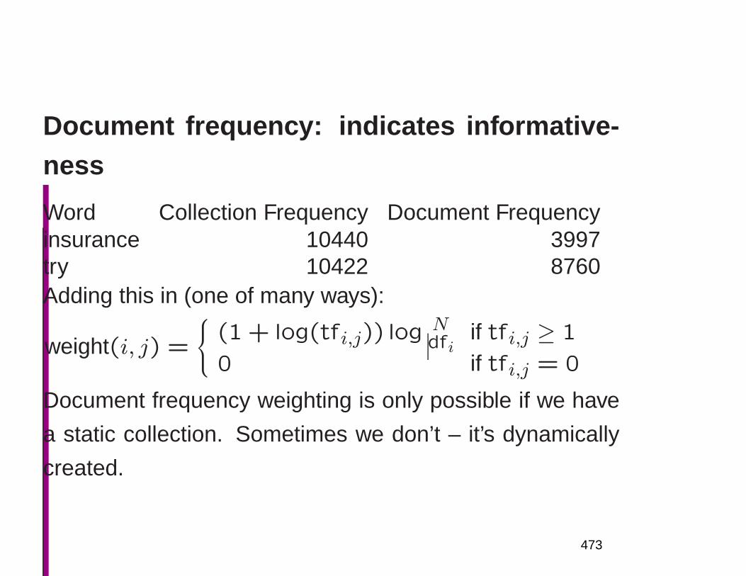
Document frequency: indicates informative-ness
Word Collection Frequency Document Frequencyinsurance 10440 3997try 10422 8760Adding this in (one of many ways):
weight(i, j) =
(1 + log(tfi,j)) log Ndfi
if tfi,j ≥ 1
0 if tfi,j = 0
Document frequency weighting is only possible if we have
a static collection. Sometimes we don’t – it’s dynamically
created.
473
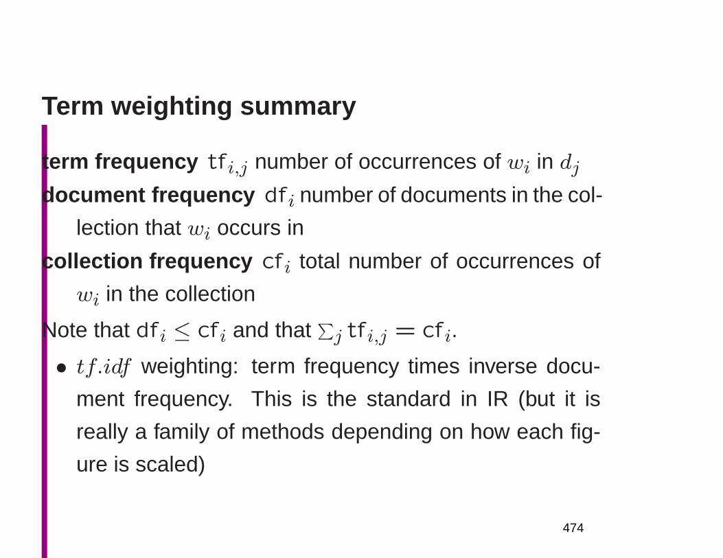
Term weighting summary
term frequency tfi,j number of occurrences of wi in djdocument frequency dfi number of documents in the col-
lection that wi occurs in
collection frequency cfi total number of occurrences of
wi in the collection
Note that dfi ≤ cfi and that∑
j tfi,j = cfi.
• tf.idf weighting: term frequency times inverse docu-
ment frequency. This is the standard in IR (but it is
really a family of methods depending on how each fig-
ure is scaled)
474
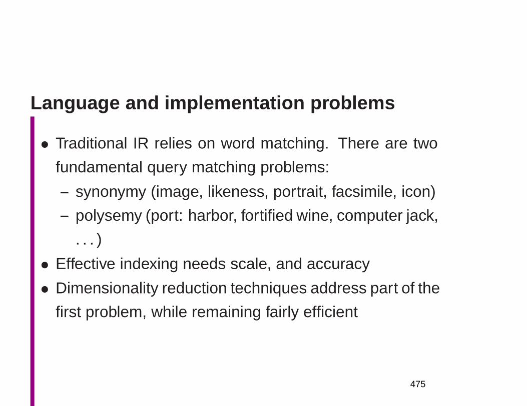
Language and implementation problems
• Traditional IR relies on word matching. There are two
fundamental query matching problems:
– synonymy (image, likeness, portrait, facsimile, icon)
– polysemy (port: harbor, fortified wine, computer jack,
. . . )
• Effective indexing needs scale, and accuracy
• Dimensionality reduction techniques address part of the
first problem, while remaining fairly efficient
475
Latent Semantic Indexing (LSI)
• Approach: Treat word-to-document association data as
an unreliable estimate of a larger set of applicable words
lying on ‘latent’ dimensions.
• Goal: Cluster similar documents which may share no
terms in a low-dimensional subspace (improve recall).
• Preprocessing: Compute low-rank approximation to the
original term-by-document (sparse) matrix
• Vector Space Model: Encode terms and documents
using factors derived from SVD
• Evaluation: Rank similarity of terms and docs to query
via Euclidean distances or cosines
476
Singular Value Decomposition Encoding
• Computes a truncated SVD of the document-term ma-
trix, using the singlular vectors as axes of the lower
dimensional space
• Ak is the best rank-k approximation to the term-by-
document matrix A
• Want minimum number of factors (k) that discriminates
most concepts
• In practice, k ranges between 100 and 300 but could
be much larger.
• Choosing optimal k for different collections is challeng-
ing.
477
Strengths and weaknesses of LSI
• Strong formal framework. Completely automatic. Nostemming required. Allows misspellings
• Can be used for multilingual search (Flournoy & PetersStanford, Landauer Colorado, Littman Duke)
• ‘Conceptual IR’ recall improvement: one can retrieverelevant documents that do not contain any search terms
• Calculation of LSI is expensive
• Continuous normal-distribution-based methods not re-ally appropriate for count data
• Often improving precision is more important: need queryand word sense disambiguation
478
Cosine, Euclidean, and Assignment 6
• Just so there are no misunderstandings. . .
• In class on Monday, I suggested that one might pre-
normalize the vectors in a vector space model
• However, for the assignment
– The data structures store integer counts and lengths,
they’re not set up for pre-normalizing
– We want you to compare the cosine measure and
Euclidean distance, and this distinction only makes
sense if you don’t pre-normalize (as we discussed)
479
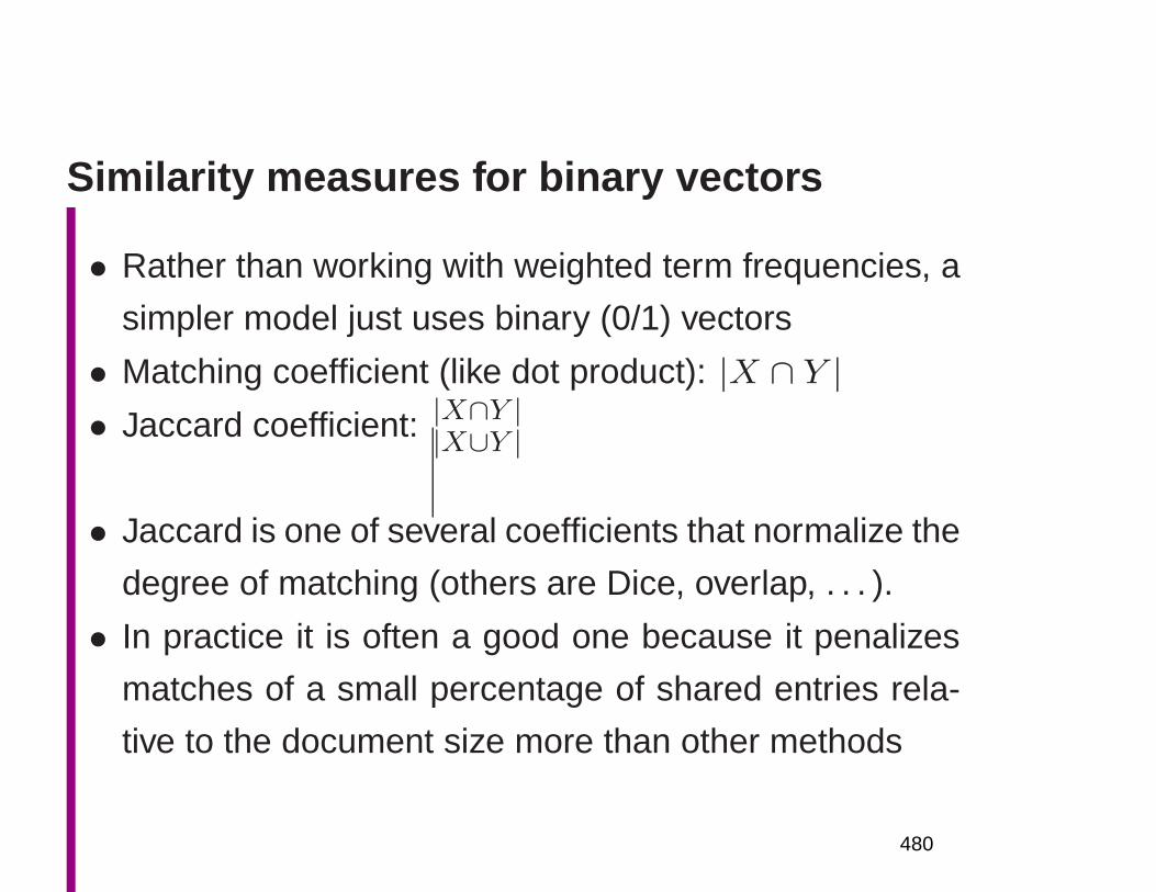
Similarity measures for binary vectors
• Rather than working with weighted term frequencies, a
simpler model just uses binary (0/1) vectors
• Matching coefficient (like dot product): |X ∩ Y |• Jaccard coefficient: |X∩Y ||X∪Y |
• Jaccard is one of several coefficients that normalize the
degree of matching (others are Dice, overlap, . . . ).
• In practice it is often a good one because it penalizes
matches of a small percentage of shared entries rela-
tive to the document size more than other methods
480
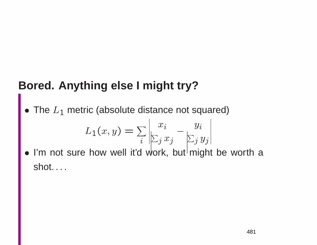
Bored. Anything else I might try?
• The L1 metric (absolute distance not squared)
L1(x, y) =∑
i
∣
∣
∣
∣
∣
∣
xi∑
j xj− yi
∑
j yj
∣
∣
∣
∣
∣
∣
• I’m not sure how well it’d work, but might be worth a
shot. . . .
481
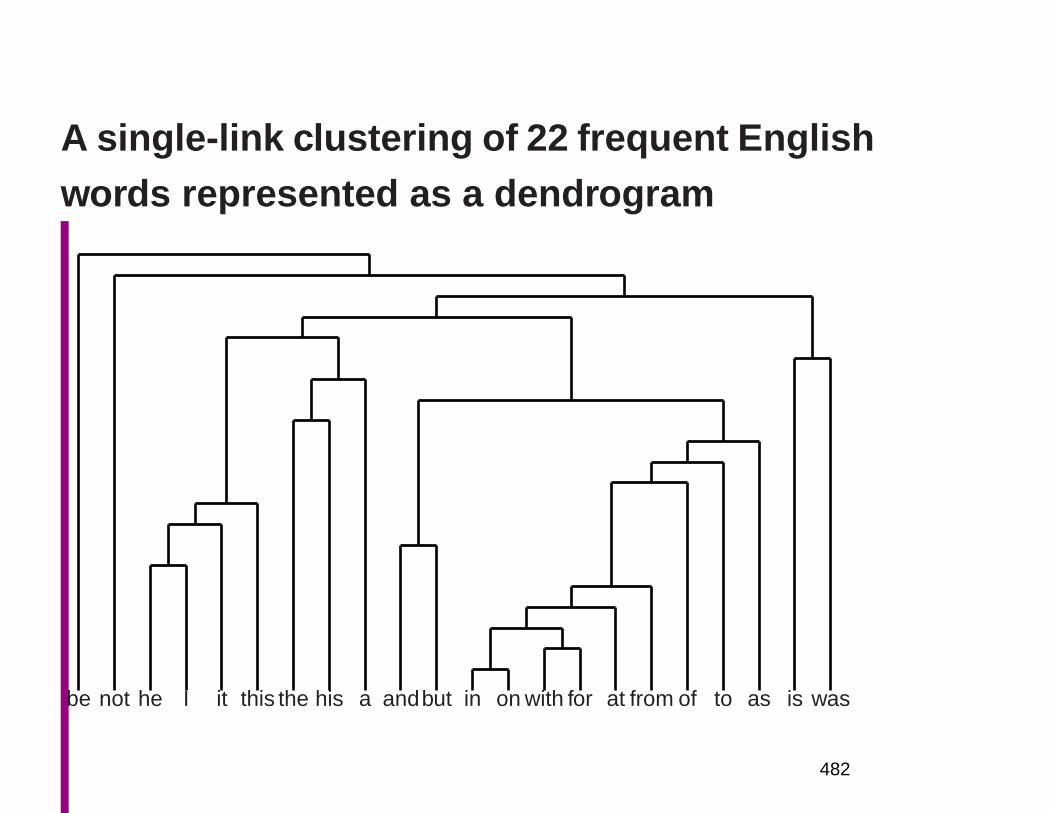
A single-link clustering of 22 frequent Englishwords represented as a dendrogram
be not he I it this the his a andbut in on with for at from of to as is was
482
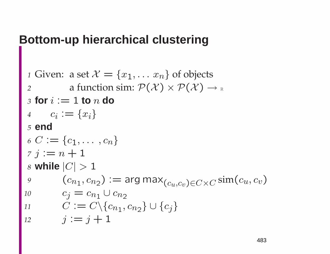
Bottom-up hierarchical clustering
1 Given: a set X = x1, . . . xn of objects2 a function sim: P(X )× P(X )→ R
3 for i := 1 to n do4 ci := xi5 end6 C := c1, . . . , cn7 j := n+ 1
8 while |C| > 1
9 (cn1, cn2) := argmax(cu,cv)∈C×C sim(cu, cv)
10 cj = cn1 ∪ cn2
11 C := C\cn1, cn2 ∪ cj12 j := j + 1
483
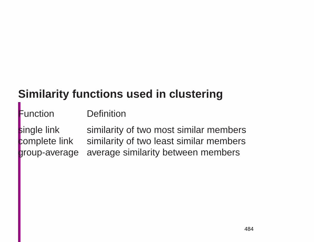
Similarity functions used in clustering
Function Definition
single link similarity of two most similar memberscomplete link similarity of two least similar membersgroup-average average similarity between members
484
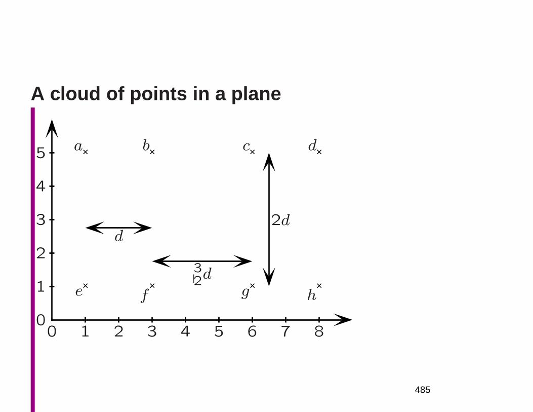
A cloud of points in a plane
0 1 2 3 4 5 6 7 80
1
2
3
4
5
×e ×f
×g ×h
×a ×b ×c ×d
32d
d2d
485
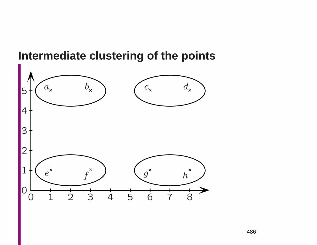
Intermediate clustering of the points
0 1 2 3 4 5 6 7 80
1
2
3
4
5
×e ×f
×g ×h
×a ×b ×c ×d
486
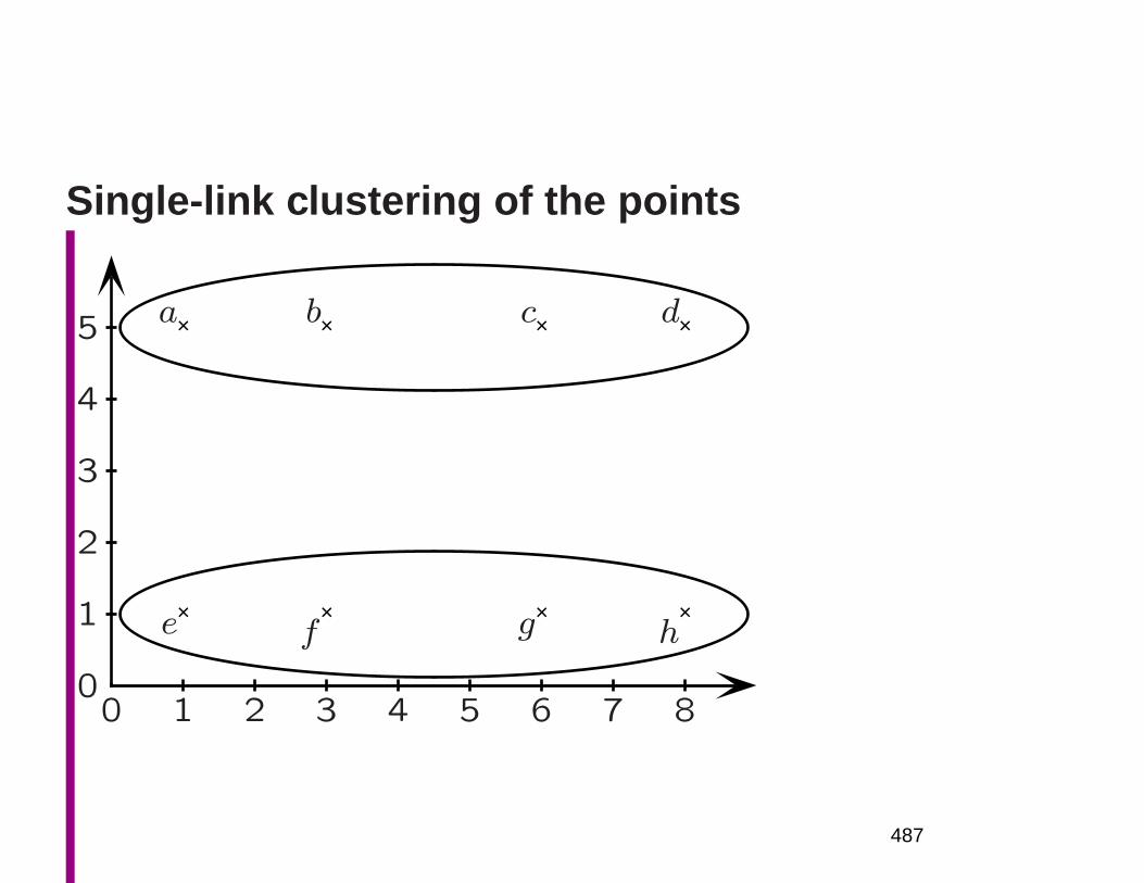
Single-link clustering of the points
0 1 2 3 4 5 6 7 80
1
2
3
4
5
×e ×f
×g ×h
×a ×b ×c ×d
487
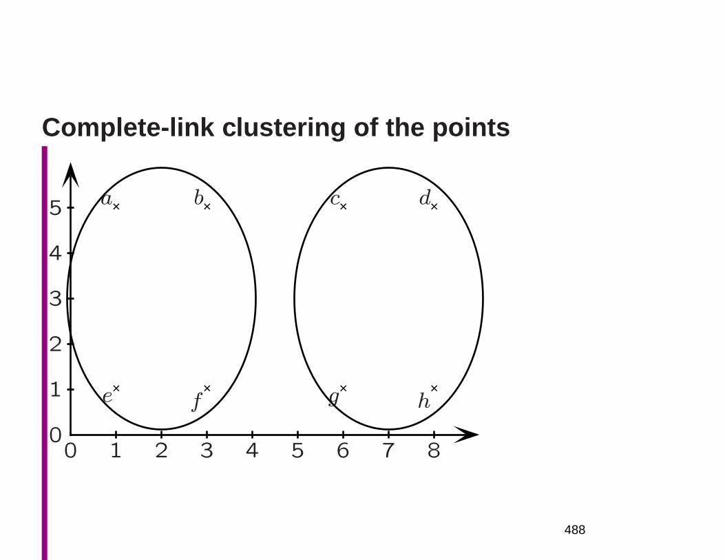
Complete-link clustering of the points
0 1 2 3 4 5 6 7 80
1
2
3
4
5
×e ×f
×g ×h
×a ×b ×c ×d
488
The EM algorithm based on a presentation by Dan Klein
• A very general and well-studied algorithm
• I cover only the specific case we use in this course:
maximum-likelihood estimation for models with discrete
hidden variables
• (For continuous case, sums go to integrals; for MAP
estimation, changes to accommodate prior)
• As an easy example we estimate parameters of an n-
gram mixture model
• For all details of EM, try McLachlan and Krishnan (1996)
489
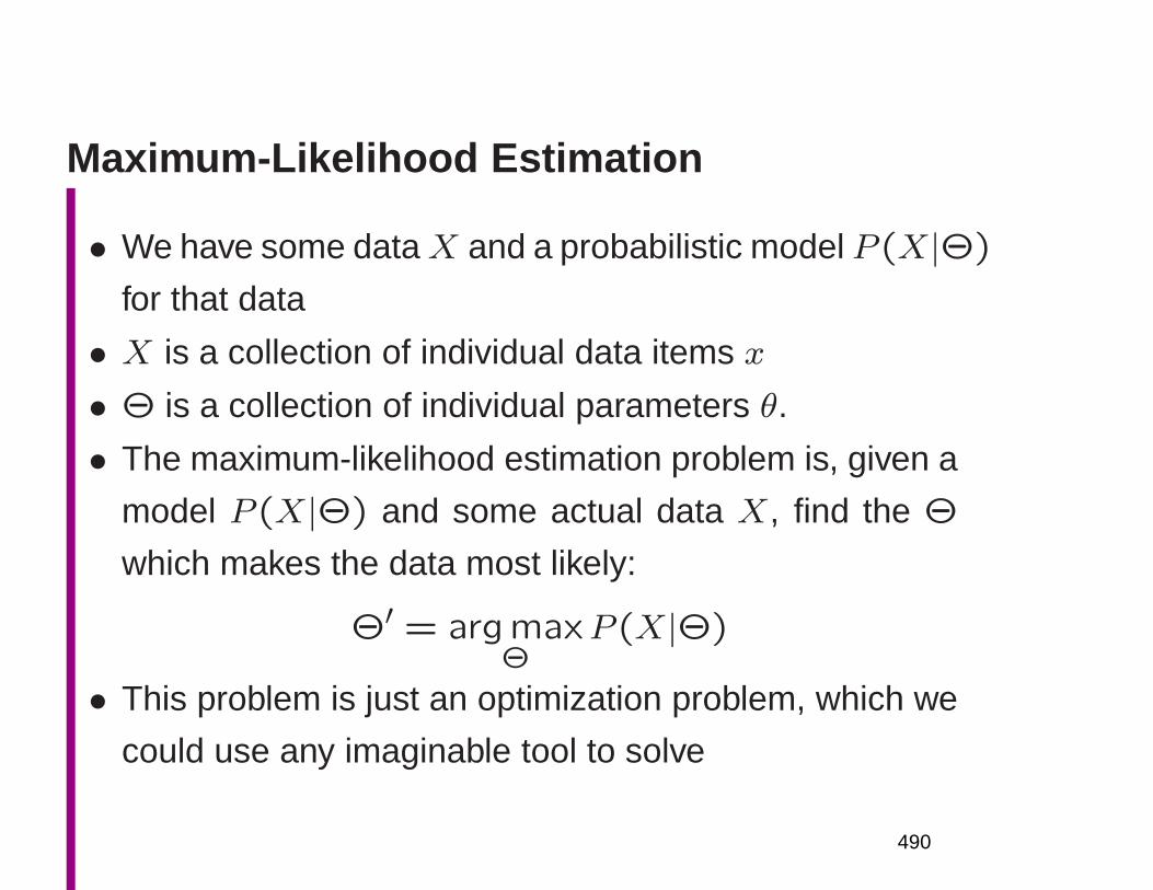
Maximum-Likelihood Estimation
• We have some dataX and a probabilistic model P (X|Θ)
for that data
• X is a collection of individual data items x
• Θ is a collection of individual parameters θ.
• The maximum-likelihood estimation problem is, given a
model P (X|Θ) and some actual data X, find the Θ
which makes the data most likely:
Θ′ = argmaxΘ
P (X|Θ)
• This problem is just an optimization problem, which we
could use any imaginable tool to solve
490
Maximum-Likelihood Estimation
• In practice, it’s often hard to get expressions for the
derivatives needed by gradient methods
• EM is one popular and powerful way of proceeding, but
not the only way.
• Remember, EM is doing MLE
491
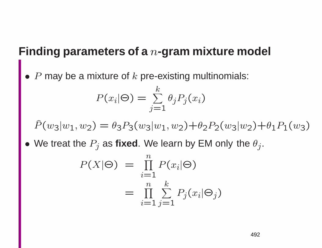
Finding parameters of a n-gram mixture model
• P may be a mixture of k pre-existing multinomials:
P (xi|Θ) =k
∑
j=1θjPj(xi)
P (w3|w1, w2) = θ3P3(w3|w1, w2)+θ2P2(w3|w2)+θ1P1(w3)
• We treat the Pj as fixed . We learn by EM only the θj.
P (X|Θ) =n∏
i=1P (xi|Θ)
=n∏
i=1
k∑
j=1Pj(xi|Θj)
492
1
• X = [x1 . . . xn] is a sequence of n words drawn from
a vocabulary V , and Θ = [θ1 . . . θk] are the mixing
weights
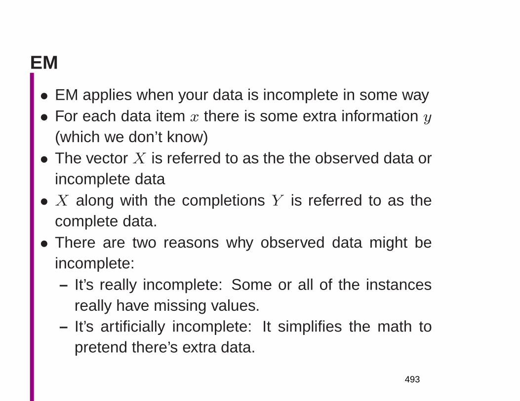
EM
• EM applies when your data is incomplete in some way• For each data item x there is some extra information y
(which we don’t know)• The vector X is referred to as the the observed data or
incomplete data• X along with the completions Y is referred to as the
complete data.• There are two reasons why observed data might be
incomplete:– It’s really incomplete: Some or all of the instances
really have missing values.– It’s artificially incomplete: It simplifies the math to
pretend there’s extra data.
493
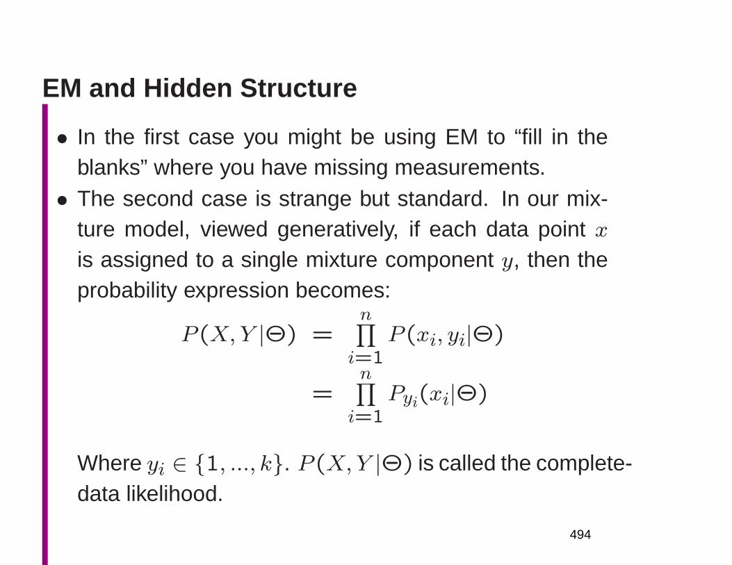
EM and Hidden Structure
• In the first case you might be using EM to “fill in theblanks” where you have missing measurements.• The second case is strange but standard. In our mix-
ture model, viewed generatively, if each data point xis assigned to a single mixture component y, then theprobability expression becomes:
P (X,Y |Θ) =n∏
i=1P (xi, yi|Θ)
=n∏
i=1Pyi(xi|Θ)
Where yi ∈ 1, ..., k. P (X,Y |Θ) is called the complete-data likelihood.
494
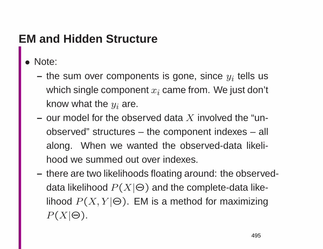
EM and Hidden Structure
• Note:
– the sum over components is gone, since yi tells uswhich single component xi came from. We just don’tknow what the yi are.
– our model for the observed data X involved the “un-observed” structures – the component indexes – allalong. When we wanted the observed-data likeli-hood we summed out over indexes.
– there are two likelihoods floating around: the observed-data likelihood P (X|Θ) and the complete-data like-lihood P (X,Y |Θ). EM is a method for maximizingP (X|Θ).
495
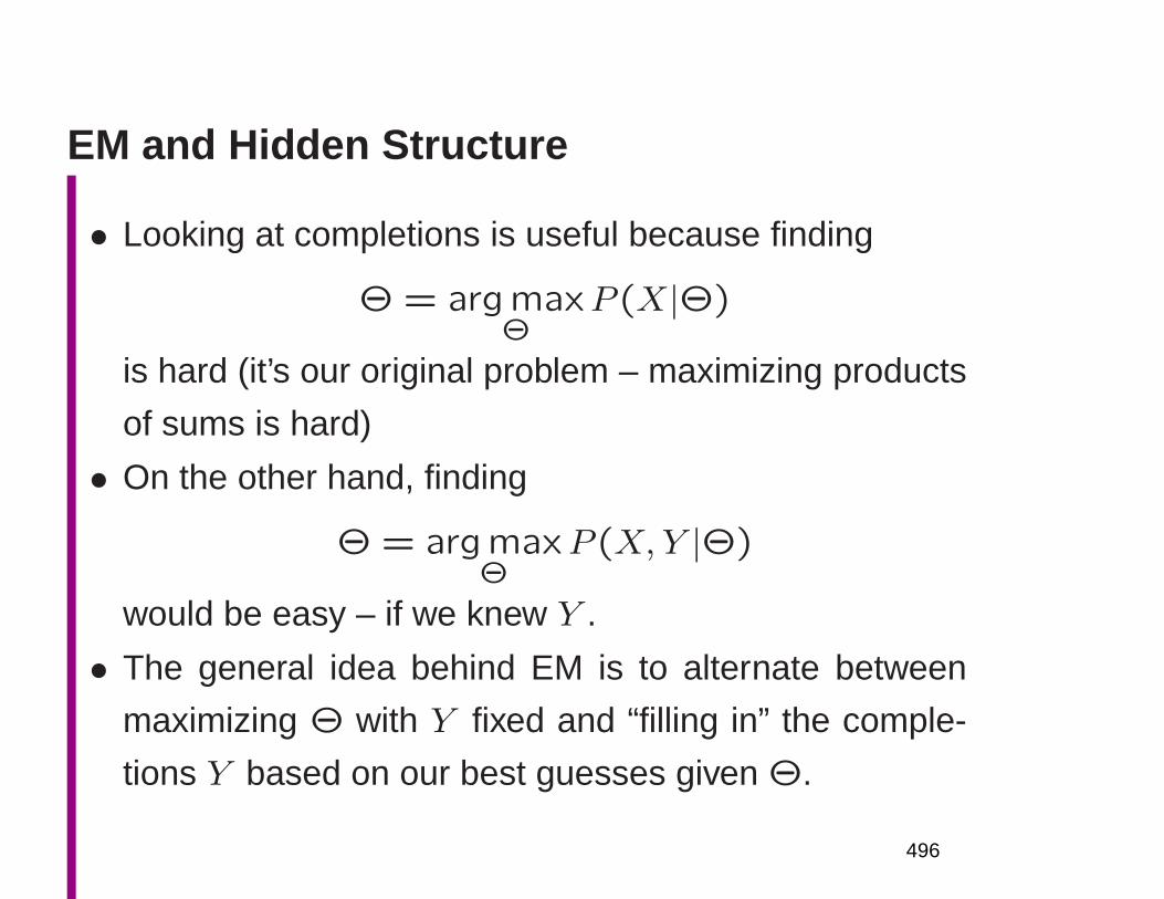
EM and Hidden Structure
• Looking at completions is useful because finding
Θ = argmaxΘ
P (X|Θ)
is hard (it’s our original problem – maximizing products
of sums is hard)
• On the other hand, finding
Θ = argmaxΘ
P (X,Y |Θ)
would be easy – if we knew Y .
• The general idea behind EM is to alternate between
maximizing Θ with Y fixed and “filling in” the comple-
tions Y based on our best guesses given Θ.
496
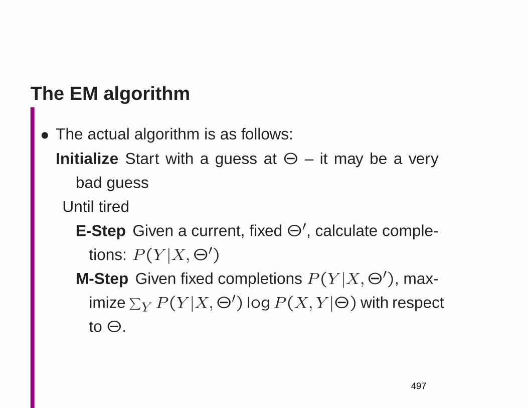
The EM algorithm
• The actual algorithm is as follows:
Initialize Start with a guess at Θ – it may be a very
bad guess
Until tired
E-Step Given a current, fixed Θ′, calculate comple-
tions: P (Y |X,Θ′)M-Step Given fixed completions P (Y |X,Θ′), max-
imize∑
Y P (Y |X,Θ′) logP (X,Y |Θ) with respect
to Θ.
497
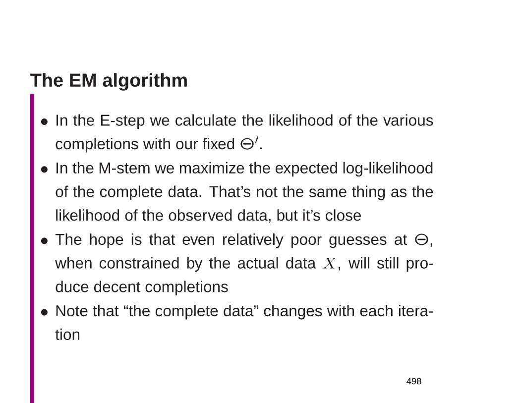
The EM algorithm
• In the E-step we calculate the likelihood of the various
completions with our fixed Θ′.• In the M-stem we maximize the expected log-likelihood
of the complete data. That’s not the same thing as the
likelihood of the observed data, but it’s close
• The hope is that even relatively poor guesses at Θ,
when constrained by the actual data X, will still pro-
duce decent completions
• Note that “the complete data” changes with each itera-
tion
498
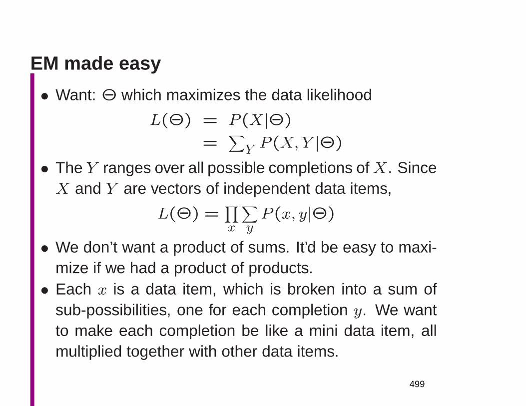
EM made easy
• Want: Θ which maximizes the data likelihood
L(Θ) = P (X|Θ)
=∑
Y P (X,Y |Θ)
• The Y ranges over all possible completions ofX. SinceX and Y are vectors of independent data items,
L(Θ) =∏
x
∑
yP (x, y|Θ)
• We don’t want a product of sums. It’d be easy to maxi-mize if we had a product of products.• Each x is a data item, which is broken into a sum of
sub-possibilities, one for each completion y. We wantto make each completion be like a mini data item, allmultiplied together with other data items.
499
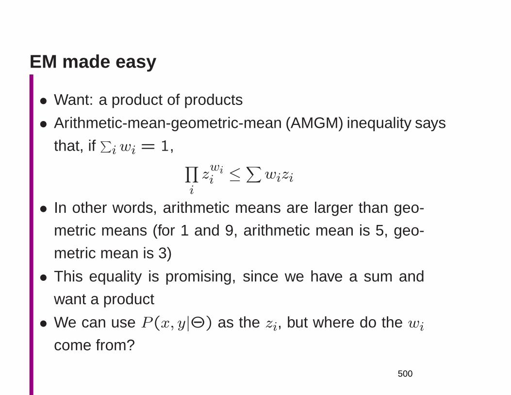
EM made easy
• Want: a product of products
• Arithmetic-mean-geometric-mean (AMGM) inequality says
that, if∑
iwi = 1,∏
izwii ≤
∑
wizi
• In other words, arithmetic means are larger than geo-
metric means (for 1 and 9, arithmetic mean is 5, geo-
metric mean is 3)
• This equality is promising, since we have a sum and
want a product
• We can use P (x, y|Θ) as the zi, but where do the wicome from?
500
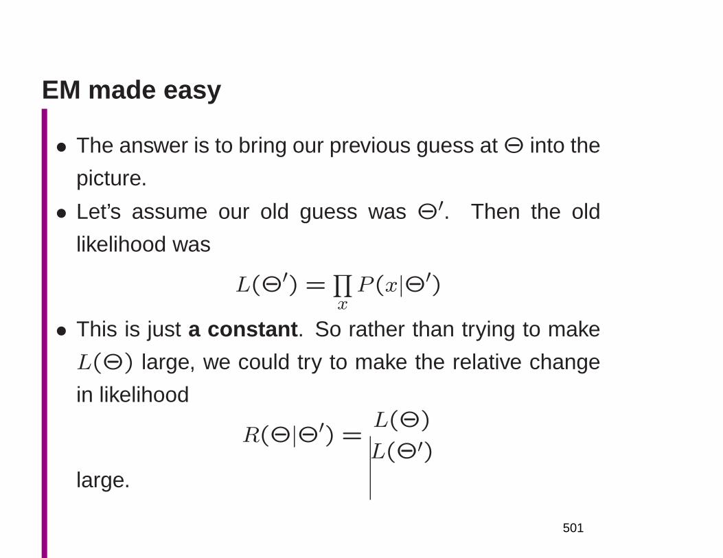
EM made easy
• The answer is to bring our previous guess at Θ into the
picture.
• Let’s assume our old guess was Θ′. Then the old
likelihood was
L(Θ′) =∏
xP (x|Θ′)
• This is just a constant . So rather than trying to make
L(Θ) large, we could try to make the relative change
in likelihood
R(Θ|Θ′) =L(Θ)
L(Θ′)large.
501
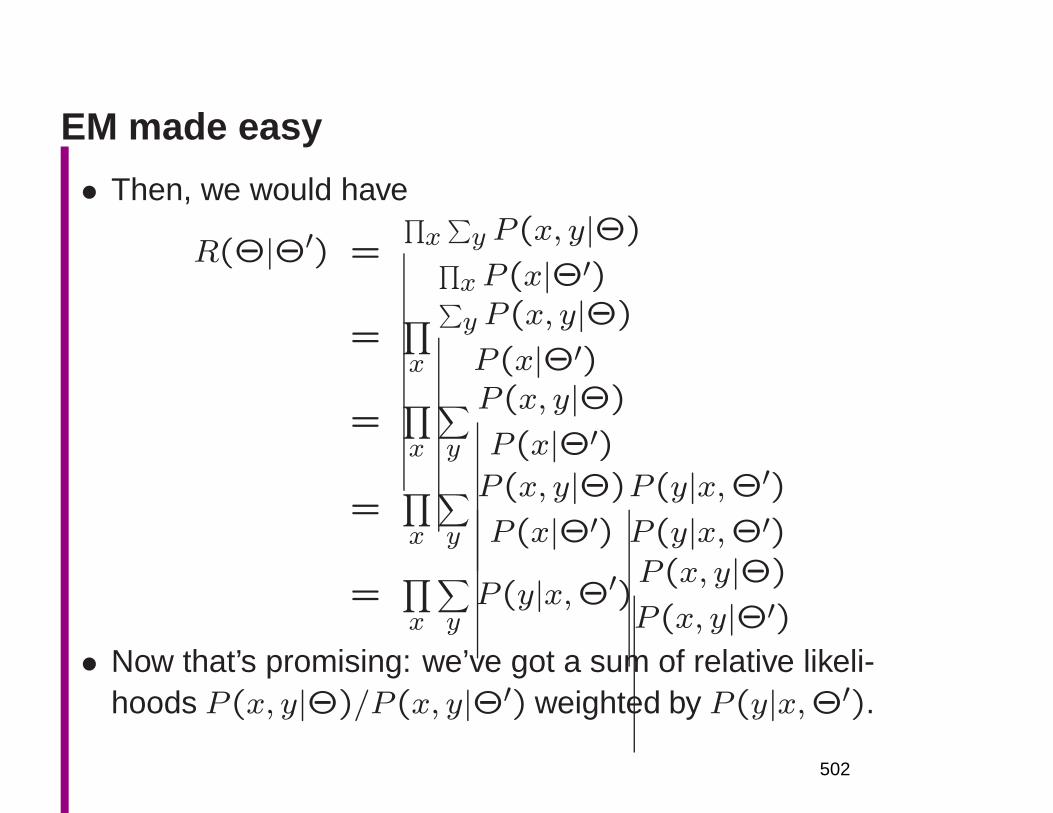
EM made easy
• Then, we would have
R(Θ|Θ′) =
∏
x∑
y P (x, y|Θ)∏
xP (x|Θ′)=
∏
x
∑
y P (x, y|Θ)
P (x|Θ′)=
∏
x
∑
y
P (x, y|Θ)
P (x|Θ′)
=∏
x
∑
y
P (x, y|Θ)
P (x|Θ′)P (y|x,Θ′)P (y|x,Θ′)
=∏
x
∑
yP (y|x,Θ′)P (x, y|Θ)
P (x, y|Θ′)• Now that’s promising: we’ve got a sum of relative likeli-
hoods P (x, y|Θ)/P (x, y|Θ′) weighted by P (y|x,Θ′).
502
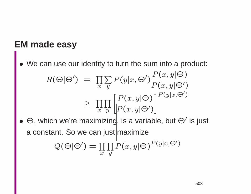
EM made easy
• We can use our identity to turn the sum into a product:
R(Θ|Θ′) =∏
x
∑
yP (y|x,Θ′)P (x, y|Θ)
P (x, y|Θ′)
≥ ∏
x
∏
y
P (x, y|Θ)
P (x, y|Θ′)
P(y|x,Θ′)
• Θ, which we’re maximizing, is a variable, but Θ′ is just
a constant. So we can just maximize
Q(Θ|Θ′) =∏
x
∏
yP (x, y|Θ)P(y|x,Θ′)
503
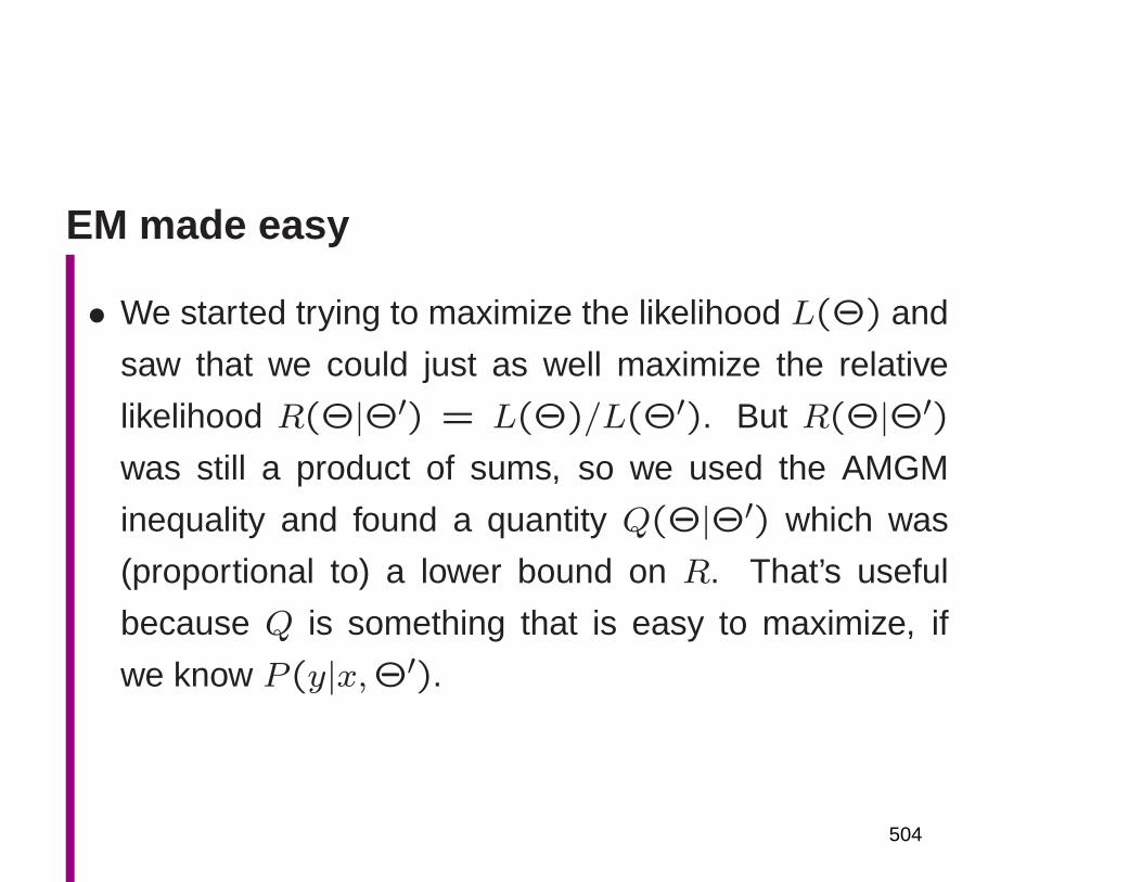
EM made easy
• We started trying to maximize the likelihood L(Θ) and
saw that we could just as well maximize the relative
likelihood R(Θ|Θ′) = L(Θ)/L(Θ′). But R(Θ|Θ′)was still a product of sums, so we used the AMGM
inequality and found a quantity Q(Θ|Θ′) which was
(proportional to) a lower bound on R. That’s useful
because Q is something that is easy to maximize, if
we know P (y|x,Θ′).
504
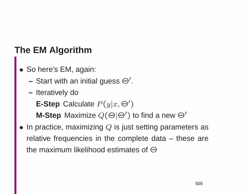
The EM Algorithm
• So here’s EM, again:
– Start with an initial guess Θ′.– Iteratively do
E-Step Calculate P (y|x,Θ′)M-Step Maximize Q(Θ|Θ′) to find a new Θ′
• In practice, maximizing Q is just setting parameters as
relative frequencies in the complete data – these are
the maximum likelihood estimates of Θ
505
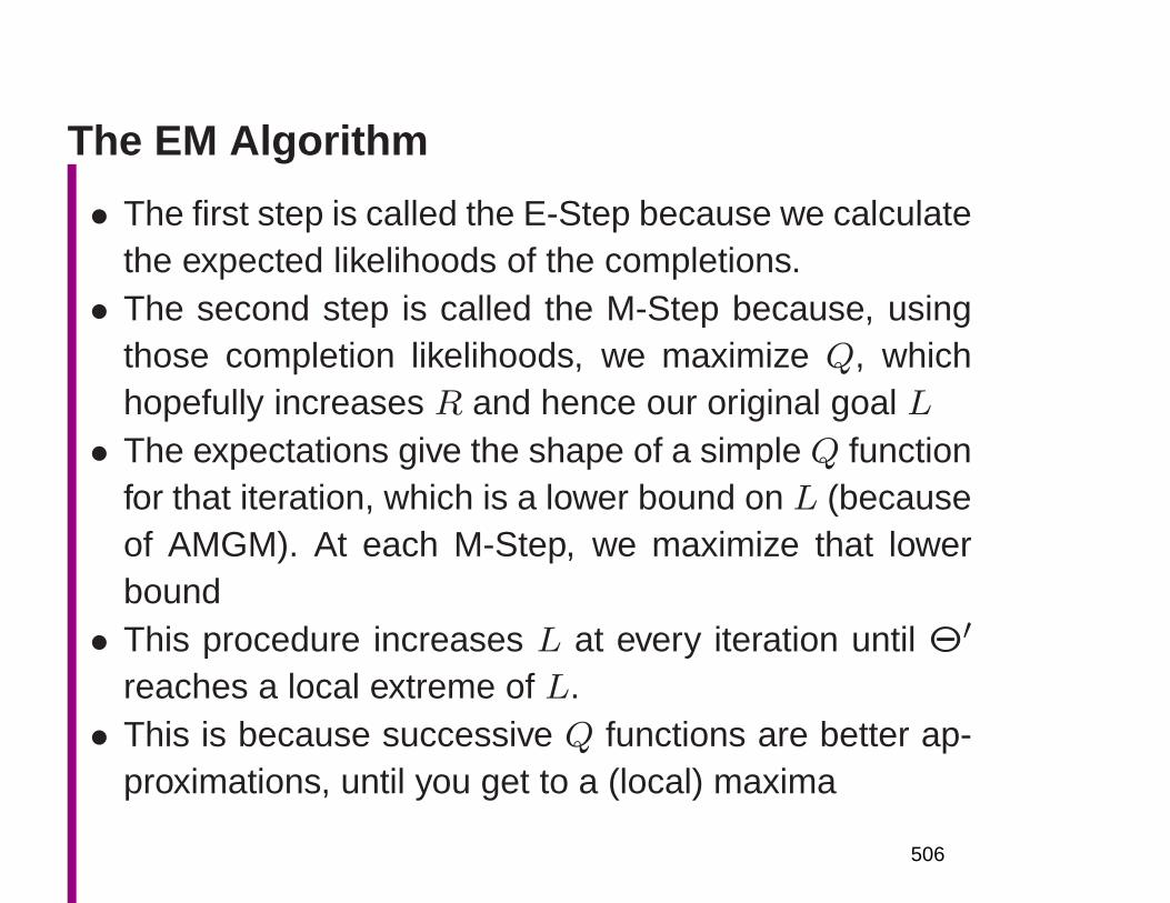
The EM Algorithm
• The first step is called the E-Step because we calculatethe expected likelihoods of the completions.• The second step is called the M-Step because, using
those completion likelihoods, we maximize Q, whichhopefully increases R and hence our original goal L• The expectations give the shape of a simple Q function
for that iteration, which is a lower bound on L (becauseof AMGM). At each M-Step, we maximize that lowerbound• This procedure increases L at every iteration until Θ′
reaches a local extreme of L.• This is because successive Q functions are better ap-
proximations, until you get to a (local) maxima
506
EM algorithm
• We initalize all parameters (randomly or intelligently)
• E-step: We work out the expectation of the hidden vari-
ables, given the current parameters for the model
• M-step: (Assuming these expectations are right), we
calculate the maximum likelihood estimates for the pa-
rameters
• Repeat until convergence
(Dempster, Laird, and Rubin 1977). Guaranteed to not
diminish the likelihood of the data according to the model.
Feasible for a large range of models (where E and M step
can be computed).
507

Text Categorization
FSNLP, chapter 16
Christopher Manning andHinrich Schütze
© 1999–2002
508

Text categorization/classification
• Take a document and assign it a label representing itstopic• Have some predefined categories for texts
– Classic example: decide if a newspaper article isabout politics, business, or sports
– Predefined categories for news items on newswires– Reuters categories
– ACM keywords– Yahoo! or Open Directory classes (extra complexity:
hierarchical)– UMLS (Unified Medical Language System) MeSH
codes• Generally approached using a bag of words model
509
Text categorization/classification
• There are many other uses for the same technology:
– Is this page a laser printer product page?
– Does this company accept overseas orders?
– What kind of job does this job posting describe?
– What kind of position does this list of responsibilities
describe?
– What position does this this list of skills best fit?
– Word sense disambiguation can actually be thought
of as text (here, context) categorization:
∗ Is this the “computer” or “harbor” sense of port?
510

Text categorization/classification
• This can be thought of as working out the “meaning”
of documents in a very primitive sense: for instance, a
news article “means” Europe and politics
• Most of the companies that claim to be understanding
your document, doing eCRM processing of your users
complaining emails, etc., are essentially offering text
categorization at the moment:
– Kana
– Autonomy
– Bhasha
– Banter
511
NLP as a classification problem
• Central to recent advances in NLP has been recon-
ceptualizing NLP as a machine learning classification
problem
• We – preferably someone else – hand-annotate data,
and then learn using standard ML methods
• Annotated data items are feature vectors ~xi with a clas-
sification ci.
• Our job is to assign an unannotated data item ~x to one
of the classes ck (or possibly to the doubt D or outlier
O categories – though in practice rarely used).
512
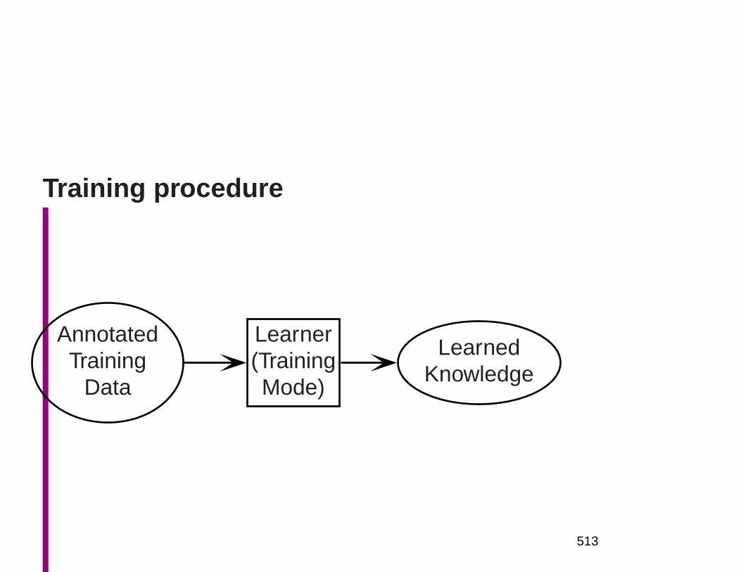
Training procedure
AnnotatedTraining
Data
Learner(TrainingMode)
LearnedKnowledge
513
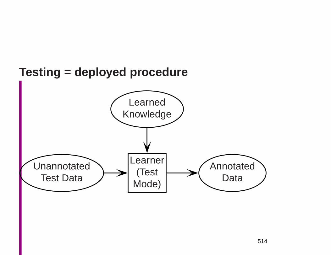
Testing = deployed procedure
UnannotatedTest Data
Learner(Test
Mode)
AnnotatedData
LearnedKnowledge
514
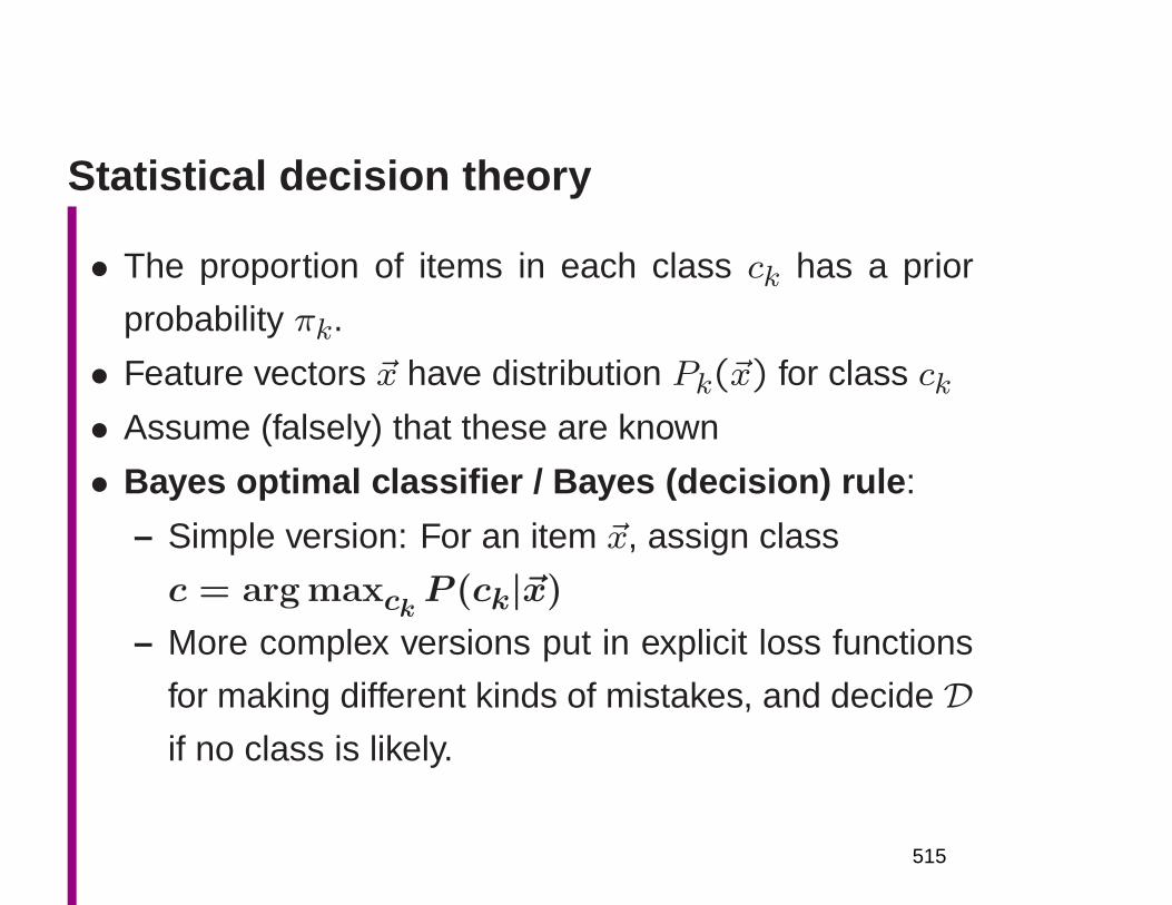
Statistical decision theory
• The proportion of items in each class ck has a prior
probability πk.
• Feature vectors ~x have distribution Pk(~x) for class ck• Assume (falsely) that these are known
• Bayes optimal classifier / Bayes (decision) rule :
– Simple version: For an item ~x, assign class
c = arg maxckP (ck|~x)
– More complex versions put in explicit loss functions
for making different kinds of mistakes, and decide Dif no class is likely.
515
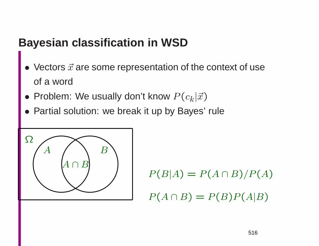
Bayesian classification in WSD
• Vectors ~x are some representation of the context of use
of a word
• Problem: We usually don’t know P (ck|~x)• Partial solution: we break it up by Bayes’ rule
A ∩B
ΩA B
P (B|A) = P (A ∩B)/P (A)
P (A ∩B) = P (B)P (A|B)
516

Bayes’ theorem
P (B|A) =P (A,B)
P (A)=P (A|B)P (B)
P (A)
If A ⊆ ∪iBi and the Bi are disjoint, then (sum rule):
P (A) =∑
iP (A,Bi) =∑
iP (A|Bi)P (Bi)
Bayes’ theorem: If A ⊆ ∪ni=1Bi, P (A) > 0, and Bi ∩Bj = ∅ for i 6= j: Likelihood Prior
P (Bj|A) =P (A|Bj)P (Bj)
P (A)=
P (A|Bj)× P (Bj)∑ni=1P (A|Bi)P (Bi)
Posterior Normalizing term
517
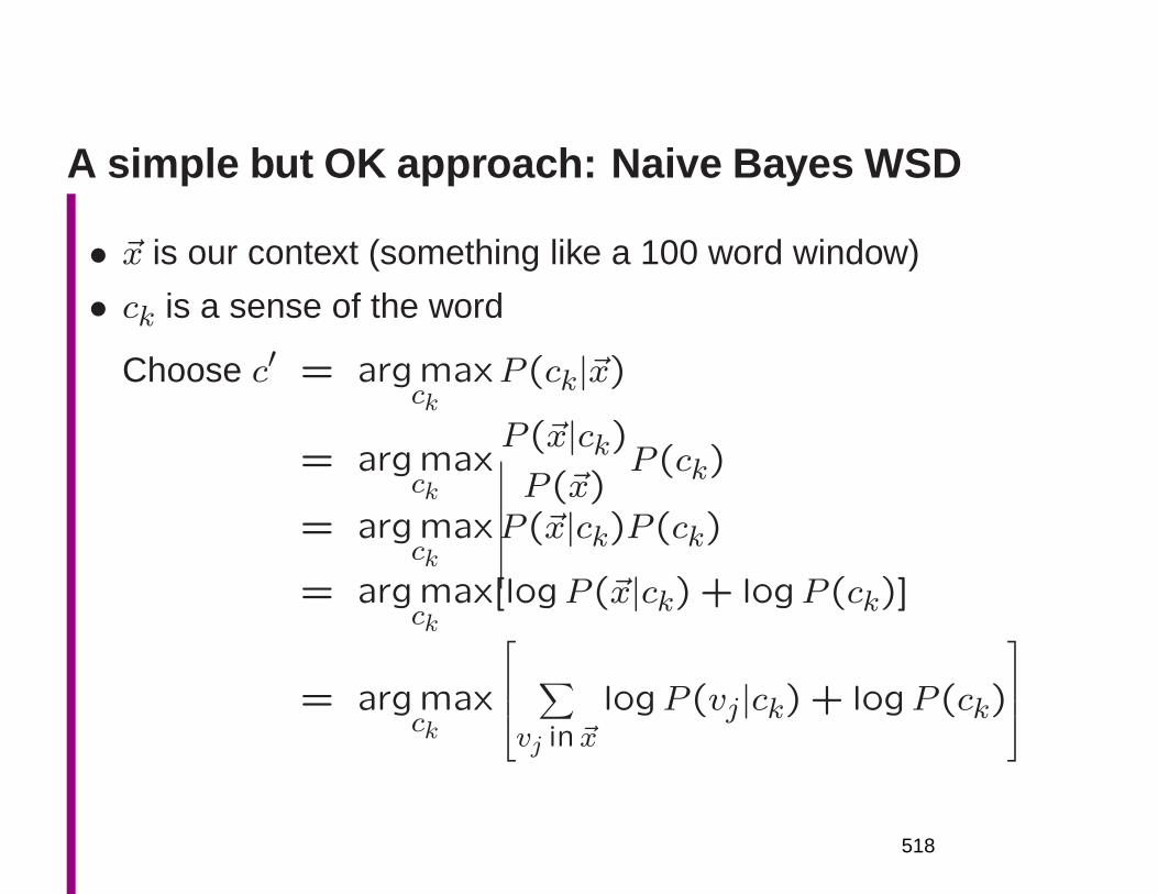
A simple but OK approach: Naive Bayes WSD
• ~x is our context (something like a 100 word window)
• ck is a sense of the word
Choose c′ = argmaxck
P (ck|~x)
= argmaxck
P (~x|ck)P (~x)
P (ck)
= argmaxck
P (~x|ck)P (ck)
= argmaxck
[logP (~x|ck) + logP (ck)]
= argmaxck
∑
vj in ~x
logP (vj|ck) + logP (ck)
518
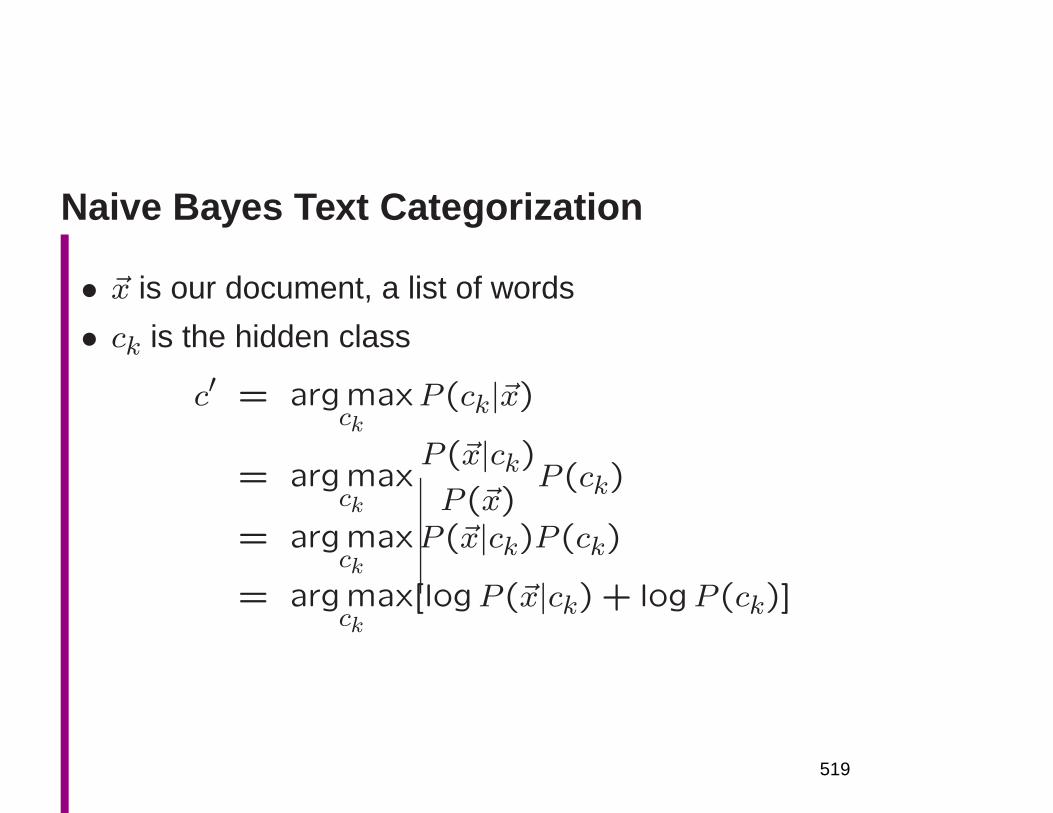
Naive Bayes Text Categorization
• ~x is our document, a list of words
• ck is the hidden class
c′ = argmaxck
P (ck|~x)
= argmaxck
P (~x|ck)P (~x)
P (ck)
= argmaxck
P (~x|ck)P (ck)
= argmaxck
[logP (~x|ck) + logP (ck)]
519
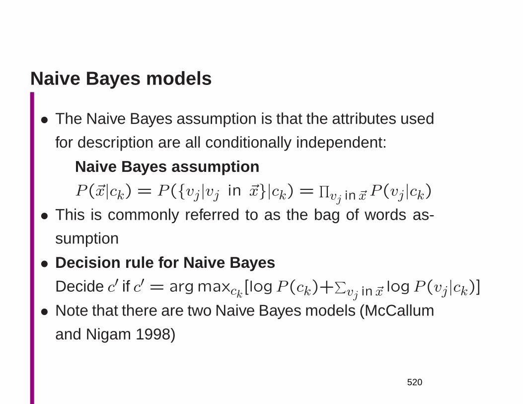
Naive Bayes models
• The Naive Bayes assumption is that the attributes used
for description are all conditionally independent:
Naive Bayes assumption
P (~x|ck) = P (vj|vj in ~x|ck) =∏
vj in ~xP (vj|ck)
• This is commonly referred to as the bag of words as-
sumption
• Decision rule for Naive Bayes
Decide c′ if c′ = argmaxck[logP (ck)+∑
vj in ~xlogP (vj|ck)]
• Note that there are two Naive Bayes models (McCallum
and Nigam 1998)
520
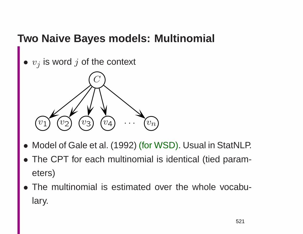
Two Naive Bayes models: Multinomial
• vj is word j of the context
C
v1 v2 v3 v4 · · · vn
• Model of Gale et al. (1992) (for WSD). Usual in StatNLP.
• The CPT for each multinomial is identical (tied param-
eters)
• The multinomial is estimated over the whole vocabu-
lary.
521

Two Naive Bayes models: Bernoulli
• wj is word (type) j of the vocabulary of features
C
w1 w2 w3 w4 · · · wV
• Each feature is binary yes/no (though could be count/range)
• Model normally presented in the graphical models liter-
ature
• Generally (but not always) performs worse
• Requires careful and aggressive feature selection
522
Naive Bayes models
• Feature selection: commonly count, χ2 or mutual infor-mation, but there are methods to find non-overlappingfeatures (Koller and Sahami 1996). Only important/relevantin Bernoulli model.
• Naive Bayes is simple, but often about as good as thereis (Friedman 1997; Domingos and Pazzani 1997)
• There are successful more complex probabilistic clas-sifiers, particularly TAN – Tree Augmented Naive Bayes(van Rijsbergen 1979; Friedman and Goldszmidt 1996)
• One can get value from varying context size accordingto type of word being disambiguated (commonly: nounis big context, verb is small context)
523

‘Typical’ McCallum and Nigam (1998) result:Reuters Money-FX category
0
20
40
60
80
100
10 100 1000 10000 100000
Pre
cisi
on/R
ecal
l Bre
akev
en P
oint
Vocabulary Size
money-fx
MultinomialMulti-variate Bernoulli
524
Text classification results
• You’ve got to be careful that you’re comparing apples
and apples
• One source of careful recent comparative studies is
Yang (1999a Information Retrieval, 1999b SIGIR)
• Results on Reuters for which several versions have been
prepared commonly differed by as great a percentage
between versions as between methods.
• Many comparisons were invalidated by data differences.
• (Should do statistical significance tests, confidence in-
tervals, . . . .)
525
Averaging
• Two ways of computing an average give very differentresults!• Micro-averaging make a single contingency table for
all the data by summing the scores in each cell for allcategories, and evaluate it– Gives equal weight to each object in the collection– Score is dominated by large categories
• Macro-averaging: compute measure for each categorycontingency table separately and then average the eval-uation measure over categories– Gives equal weight to each category– Gives a better sense of the quality of classification
across all categories.
526
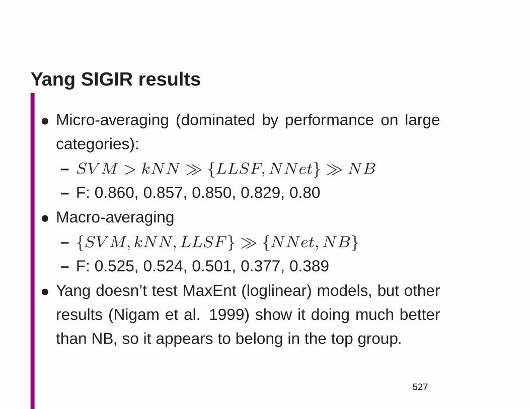
Yang SIGIR results
• Micro-averaging (dominated by performance on large
categories):
– SVM > kNN ≫ LLSF,NNet ≫ NB
– F: 0.860, 0.857, 0.850, 0.829, 0.80
• Macro-averaging
– SVM, kNN,LLSF ≫ NNet,NB– F: 0.525, 0.524, 0.501, 0.377, 0.389
• Yang doesn’t test MaxEnt (loglinear) models, but other
results (Nigam et al. 1999) show it doing much better
than NB, so it appears to belong in the top group.
527
Memory-Based Learning (MBL)/kNN
• Case-based, exemplar-based or instance-based learn-ing• A non-parametric method: no abstract model is created• Training: just store the data (indexed!)• Generalization: target function is estimated locally.• The method is not aware of the global shape of the
data, but does not make any assumptions about itsshape• Non-linear classifier• “The cost for computation is decreasing roughly by a
factor of two every year, whereas the price paid for in-correct assumptions is remaining the same.” (Breimanand Friedman 1988)
528
MBL training and testing
• “We should never underestimate the power of simply
remembering some or all of the examples and com-
paring test examples with our memory” (Ripley 1996)
Pattern Recognition and Neural Networks ← a good
book!
• Asymptotically, under various reasonable assumptions,
risk converges to twice the Bayes risk as sample grows
– independent of distance metric (Duda and Hart 1973;
Ripley 1996)
– Bayes risk = optimal error rate, assuming that prob-
ability distribution is known
529
MBL: similarity function
• Need distance function to calculate similarity
• In practice the metric is important
• Usually use Euclidean metric (alternatives Mahalanobis
distance, L1 distance = features different, etc.)
• Appropriate scaling of the variables first is important:
normalize values, sometimes log-scale etc. Can put
knowledge into metric.
530
MBL
• For 1NN decision surface is Voronoi diagram.
• Commonly distance-weight the classes of the neigh-
bors in reaching a decision
– e.g., information gain weighting used in TiMBL (Tilburg
Memory-based Learner http://ilk.kub.nl/software.html)
• Asymptotically this doesn’t help, but can allow use of
larger k for fixed size training set
• k > 1 increases resistance to noise (decreases vari-
ance)
531
Feature selection for MBL
• Excluding features which have little or no relevance is
very important
• Wrapper methods generate candidate features by test-
ing performance of the classifier with those features
• Filter methods decide features independently of algo-
rithm that will use them
• Can use decision tree techniques to select features (Cardie
1993)
532
MBL
• Naive storage and search for neighbors can be expen-
sive
• But there are efficient algorithms for indexing and hence
finding neighbors (k-d trees)
• The stored data set size can be reduced by data editing
so as to only store examples near decision surfaces.
533
Example: Part-of-Speech Tagging (Daelemanset al. 1996). Accuracy: 96.4%
• Similarity: Hamming distance (1 − %matching) = L1
norm = overlap
• Feature weighting: Information gain
• Known and unknown word models
• If known case, base features for training are:
– disambiguated ti−2, disambiguated ti−1
– ambiguity class for wi– ambiguity class for wi+1
534
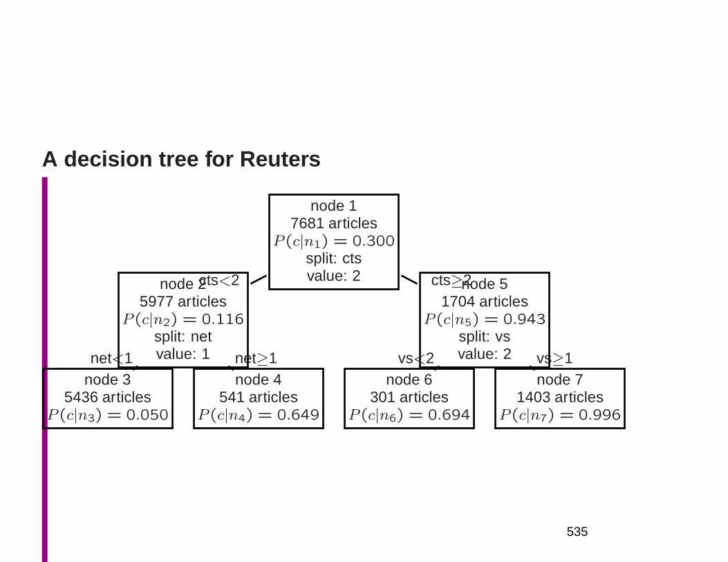
A decision tree for Reuters
node 17681 articles
P (c|n1) = 0.300split: ctsvalue: 2node 2
5977 articlesP (c|n2) = 0.116
split: netvalue: 1
cts<2
node 35436 articles
P (c|n3) = 0.050
net<1node 4
541 articlesP (c|n4) = 0.649
net≥1
node 51704 articles
P (c|n5) = 0.943split: vsvalue: 2
cts≥2
node 6301 articles
P (c|n6) = 0.694
vs<2node 7
1403 articlesP (c|n7) = 0.996
vs≥1
535
(Statistical) Decision Tree Models
• Relatively unused in statistics and pattern recognition
but introduced by Breiman et al. (1984)
• Widely used in AI machine learning (Quinlan 1986)
• Mainly because they are extremely easy to compre-
hend
• Not very efficient in combining independent information
sources
• Idea is to successively test an attribute, and then branch
based on its value
536
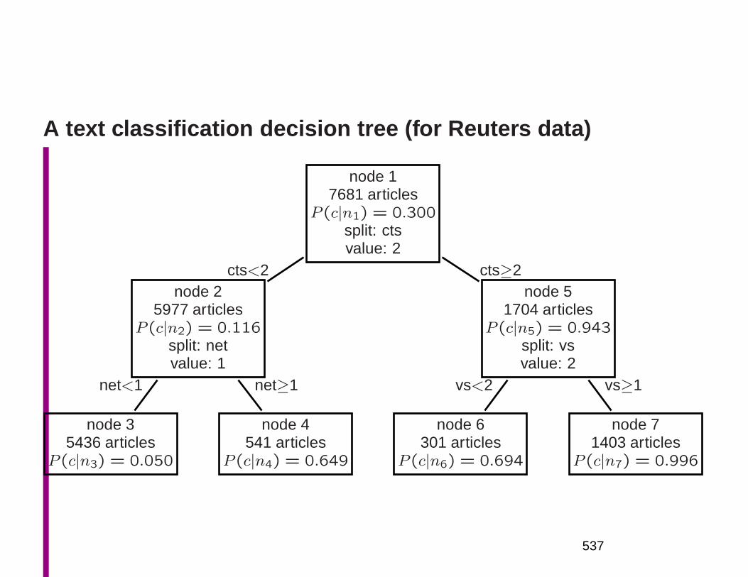
A text classification decision tree (for Reuters data)
node 17681 articles
P (c|n1) = 0.300split: ctsvalue: 2
node 25977 articles
P (c|n2) = 0.116split: netvalue: 1
cts<2
node 35436 articles
P (c|n3) = 0.050
net<1
node 4541 articles
P (c|n4) = 0.649
net≥1
node 51704 articles
P (c|n5) = 0.943split: vsvalue: 2
cts≥2
node 6301 articles
P (c|n6) = 0.694
vs<2
node 71403 articles
P (c|n7) = 0.996
vs≥1
537
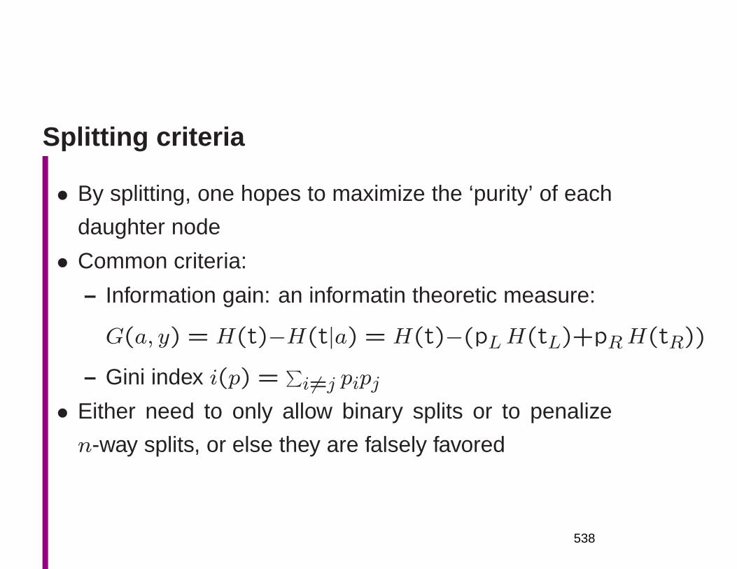
Splitting criteria
• By splitting, one hopes to maximize the ‘purity’ of each
daughter node
• Common criteria:
– Information gain: an informatin theoretic measure:
G(a, y) = H(t)−H(t|a) = H(t)−(pLH(tL)+pRH(tR))
– Gini index i(p) =∑
i 6=j pipj
• Either need to only allow binary splits or to penalize
n-way splits, or else they are falsely favored
538
Statistical decision trees
• Conserve data by only asking relevant questions
• However, since each split in the tree lessens the amount
of data, one needs a pruning strategy to prevent over
training
• A decision tree’s questions pick out boxed shaped re-
gions of the feature hyperspace
• Practically decision trees work well, though there aren’t
a lot of deep theorems to justify their performance
539
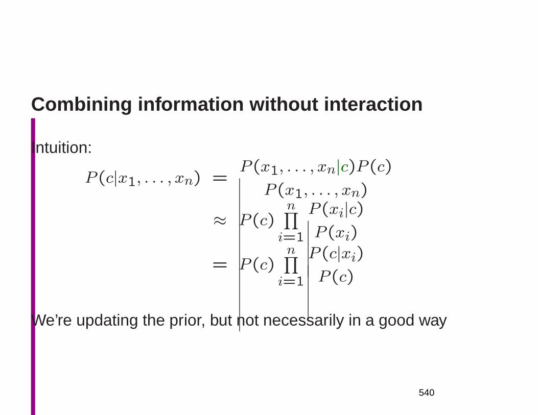
Combining information without interaction
Intuition:
P (c|x1, . . . , xn) =P (x1, . . . , xn|c)P (c)
P (x1, . . . , xn)
≈ P (c)n∏
i=1
P (xi|c)P (xi)
= P (c)n∏
i=1
P (c|xi)P (c)
We’re updating the prior, but not necessarily in a good way
540
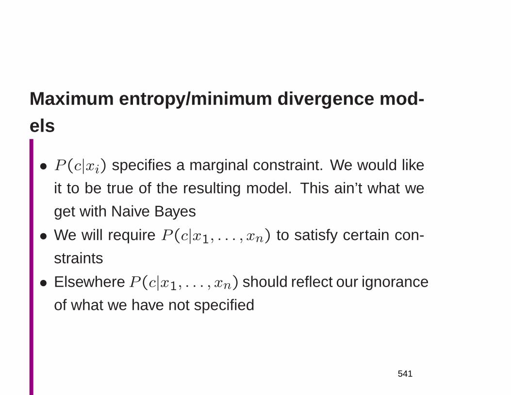
Maximum entropy/minimum divergence mod-els
• P (c|xi) specifies a marginal constraint. We would like
it to be true of the resulting model. This ain’t what we
get with Naive Bayes
• We will require P (c|x1, . . . , xn) to satisfy certain con-
straints
• Elsewhere P (c|x1, . . . , xn) should reflect our ignorance
of what we have not specified
541
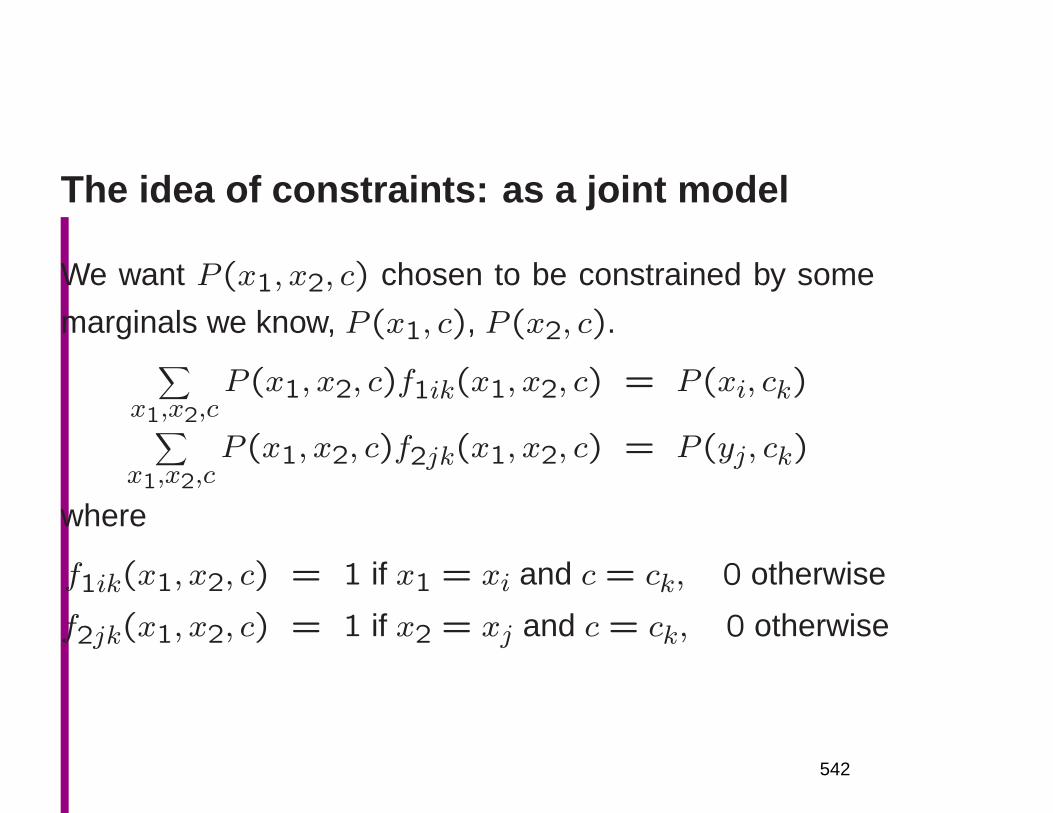
The idea of constraints: as a joint model
We want P (x1, x2, c) chosen to be constrained by some
marginals we know, P (x1, c), P (x2, c).∑
x1,x2,cP (x1, x2, c)f1ik(x1, x2, c) = P (xi, ck)
∑
x1,x2,cP (x1, x2, c)f2jk(x1, x2, c) = P (yj, ck)
where
f1ik(x1, x2, c) = 1 if x1 = xi and c = ck, 0 otherwise
f2jk(x1, x2, c) = 1 if x2 = xj and c = ck, 0 otherwise
542
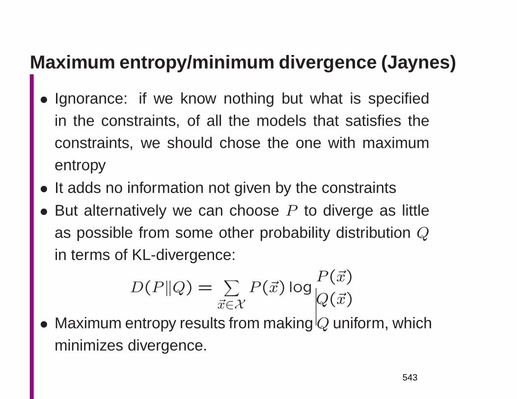
Maximum entropy/minimum divergence (Jaynes)
• Ignorance: if we know nothing but what is specifiedin the constraints, of all the models that satisfies theconstraints, we should chose the one with maximumentropy
• It adds no information not given by the constraints
• But alternatively we can choose P to diverge as littleas possible from some other probability distribution Qin terms of KL-divergence:
D(P‖Q) =∑
~x∈XP (~x) log
P (~x)
Q(~x)
• Maximum entropy results from makingQ uniform, whichminimizes divergence.
543
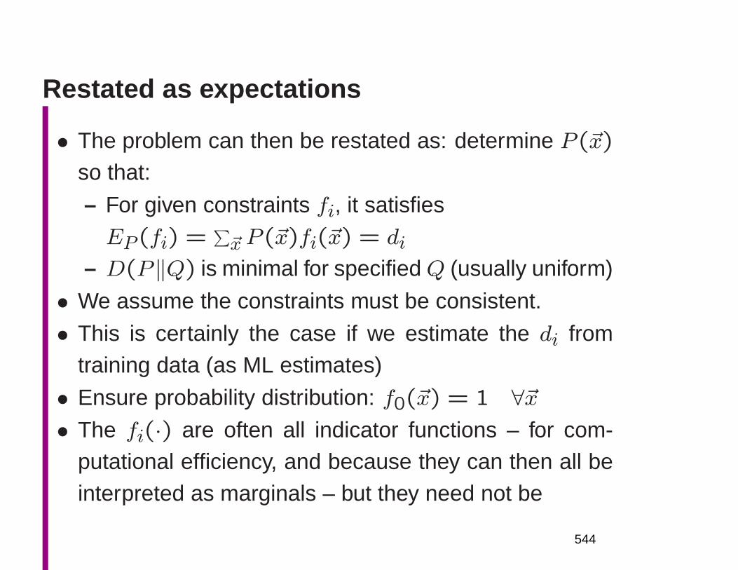
Restated as expectations
• The problem can then be restated as: determine P (~x)
so that:
– For given constraints fi, it satisfiesEP(fi) =
∑
~x P (~x)fi(~x) = di– D(P‖Q) is minimal for specifiedQ (usually uniform)
• We assume the constraints must be consistent.
• This is certainly the case if we estimate the di fromtraining data (as ML estimates)
• Ensure probability distribution: f0(~x) = 1 ∀~x• The fi(·) are often all indicator functions – for com-
putational efficiency, and because they can then all beinterpreted as marginals – but they need not be
544
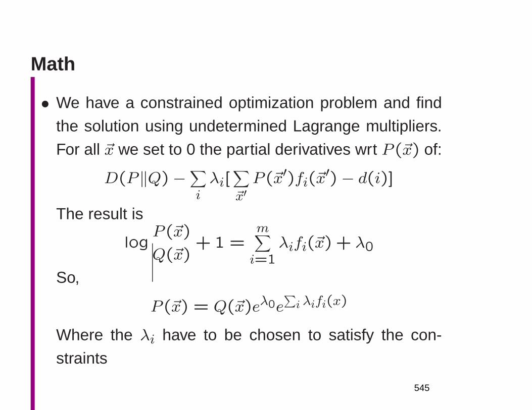
Math
• We have a constrained optimization problem and find
the solution using undetermined Lagrange multipliers.
For all ~x we set to 0 the partial derivatives wrt P (~x) of:
D(P‖Q)−∑
iλi[
∑
~x′P (~x′)fi(~x′)− d(i)]
The result is
logP (~x)
Q(~x)+ 1 =
m∑
i=1λifi(~x) + λ0
So,
P (~x) = Q(~x)eλ0e∑
i λifi(x)
Where the λi have to be chosen to satisfy the con-
straints
545
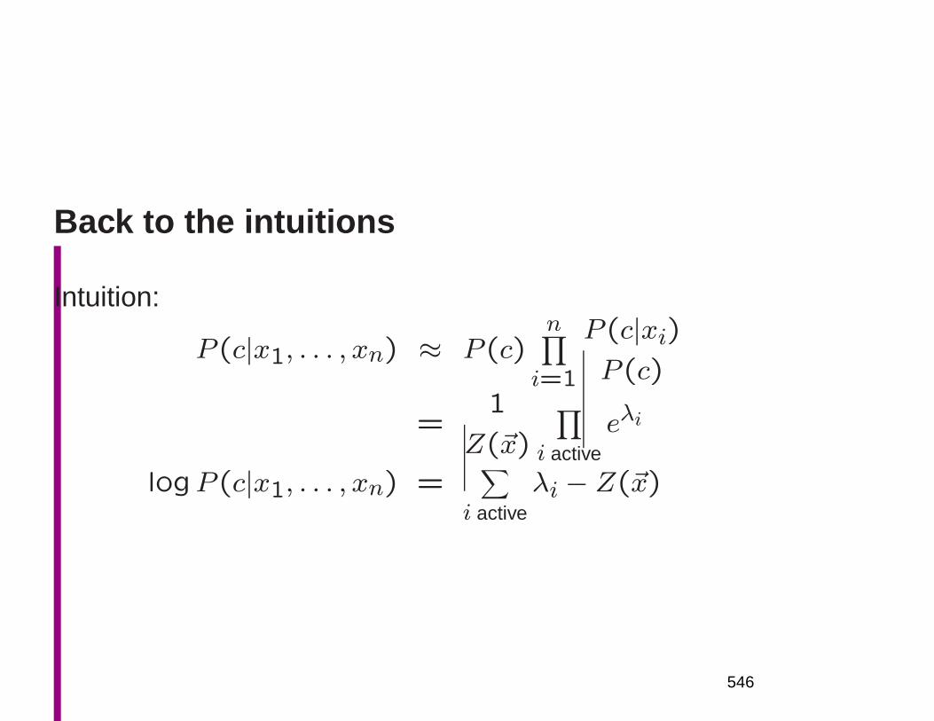
Back to the intuitions
Intuition:
P (c|x1, . . . , xn) ≈ P (c)n∏
i=1
P (c|xi)P (c)
=1
Z(~x)
∏
i activeeλi
logP (c|x1, . . . , xn) =∑
i activeλi − Z(~x)
546
Maximum entropy methods
• A unified framework for resolving ambiguities
• Can flexibly integrate heterogeneous sources of infor-
mation
• Quite high performance tools can be built fairly quickly
and automatically
• Basic algorithm is reusable; main need is annotated
training data
547
Advantages
• If features don’t overlap, exponential models can imi-
tate other models
• If features do overlap, exponential models can perform
better
– They discount weights for overlap
– But they don’t automatically model complex feature
interactions
548

Maximum entropy features
• ‘Features’ include the class assignment
• For classification, a feature f has the form fi(~x, c)
• ~x is what we observe (e.g., words)
• c is what we are predicting (e.g., tags)
• Each feature is a constraint on the model
• E.g., we might have fHAVE,VBN = 1 iff the word’s cur-
rent tag is classified as VBN, and the previous verb’s
features says it’s a perfective have auxiliary
549
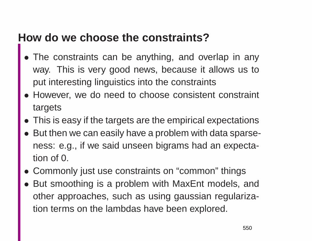
How do we choose the constraints?
• The constraints can be anything, and overlap in anyway. This is very good news, because it allows us toput interesting linguistics into the constraints• However, we do need to choose consistent constraint
targets• This is easy if the targets are the empirical expectations• But then we can easily have a problem with data sparse-
ness: e.g., if we said unseen bigrams had an expecta-tion of 0.• Commonly just use constraints on “common” things• But smoothing is a problem with MaxEnt models, and
other approaches, such as using gaussian regulariza-tion terms on the lambdas have been explored.
550
Maximum entropy model
• We compute expectation of each feature based on train-
ing set (if feature is binary this is just relative frequency)
• Say that this empirical expectation must be met in re-
sulting model→ the constraints
• We then compute model with maximum entropy subject
to the constraints
• I.e., we don’t go beyond the data by adding information
not justified by the constraints.
551
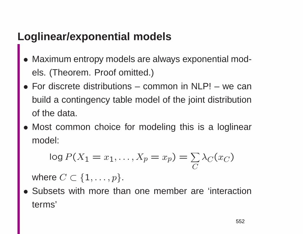
Loglinear/exponential models
• Maximum entropy models are always exponential mod-
els. (Theorem. Proof omitted.)
• For discrete distributions – common in NLP! – we can
build a contingency table model of the joint distribution
of the data.
• Most common choice for modeling this is a loglinear
model:
logP (X1 = x1, . . . ,Xp = xp) =∑
CλC(xC)
where C ⊂ 1, . . . , p.• Subsets with more than one member are ‘interaction
terms’
552
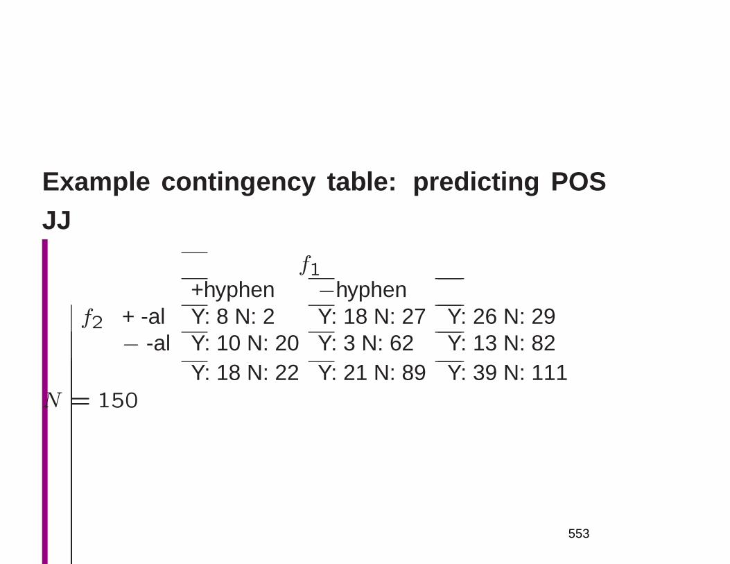
Example contingency table: predicting POSJJ
f1+hyphen −hyphen
f2 + -al Y: 8 N: 2 Y: 18 N: 27 Y: 26 N: 29− -al Y: 10 N: 20 Y: 3 N: 62 Y: 13 N: 82
Y: 18 N: 22 Y: 21 N: 89 Y: 39 N: 111N = 150
553
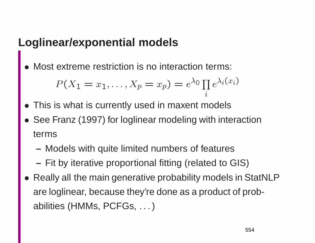
Loglinear/exponential models
• Most extreme restriction is no interaction terms:
P (X1 = x1, . . . , Xp = xp) = eλ0∏
ieλi(xi)
• This is what is currently used in maxent models
• See Franz (1997) for loglinear modeling with interaction
terms
– Models with quite limited numbers of features
– Fit by iterative proportional fitting (related to GIS)
• Really all the main generative probability models in StatNLP
are loglinear, because they’re done as a product of prob-
abilities (HMMs, PCFGs, . . . )
554
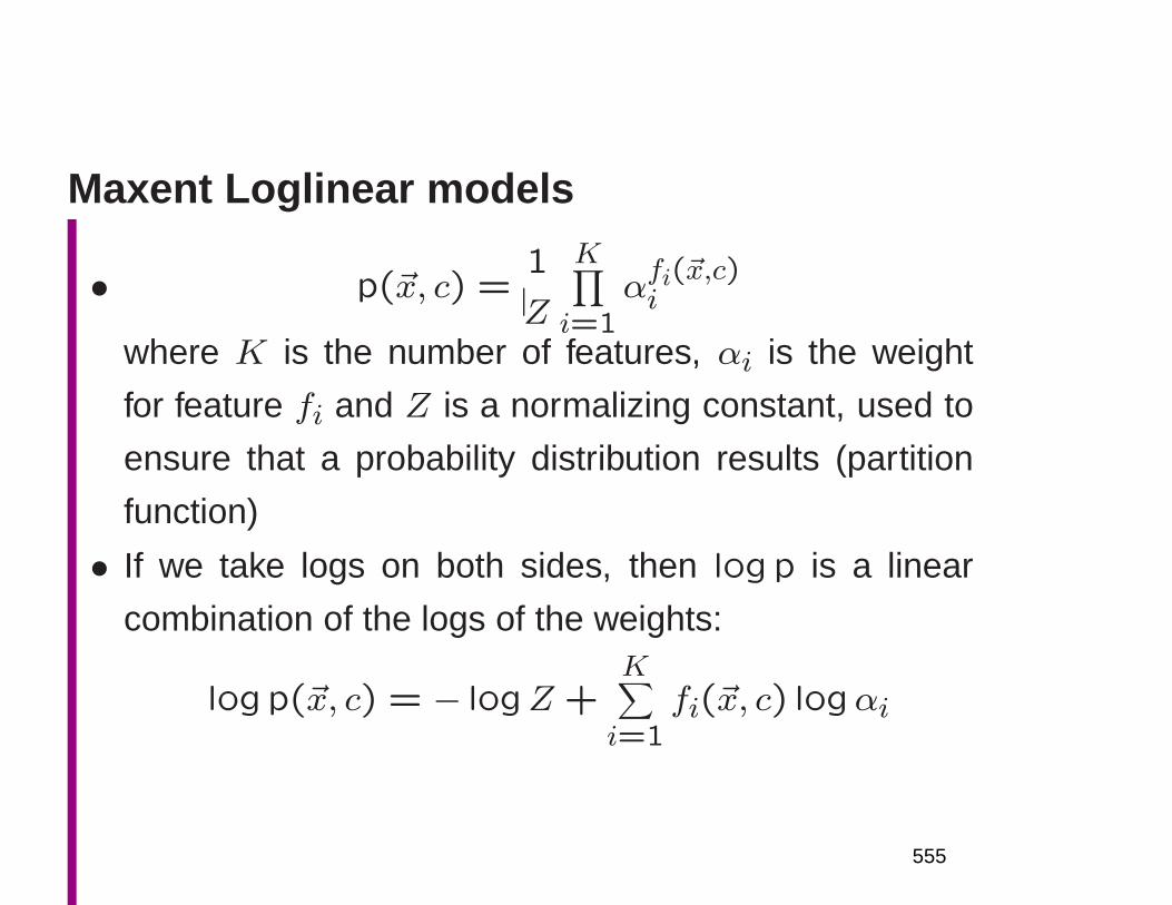
Maxent Loglinear models
• p(~x, c) =1
Z
K∏
i=1αfi(~x,c)i
where K is the number of features, αi is the weight
for feature fi and Z is a normalizing constant, used to
ensure that a probability distribution results (partition
function)
• If we take logs on both sides, then log p is a linear
combination of the logs of the weights:
log p(~x, c) = − logZ +K∑
i=1fi(~x, c) logαi
555
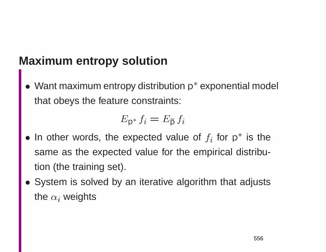
Maximum entropy solution
• Want maximum entropy distribution p∗ exponential model
that obeys the feature constraints:
Ep∗ fi = Ep fi
• In other words, the expected value of fi for p∗ is the
same as the expected value for the empirical distribu-
tion (the training set).
• System is solved by an iterative algorithm that adjusts
the αi weights
556
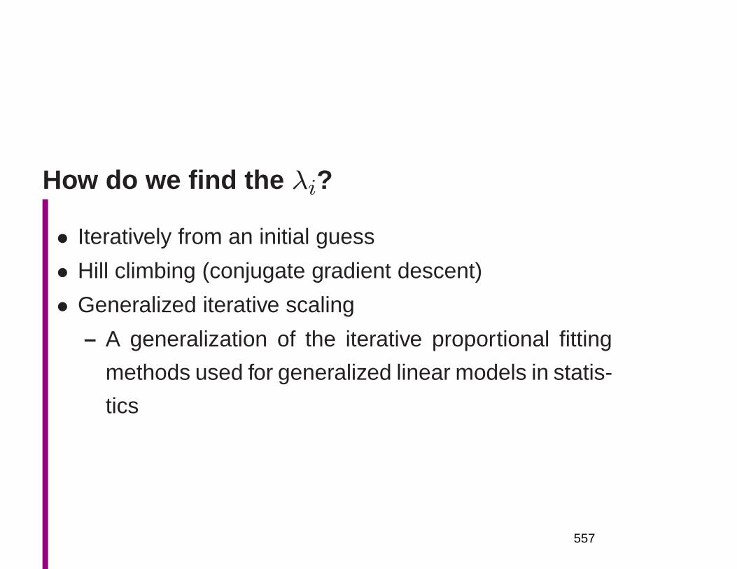
How do we find the λi?
• Iteratively from an initial guess
• Hill climbing (conjugate gradient descent)
• Generalized iterative scaling
– A generalization of the iterative proportional fitting
methods used for generalized linear models in statis-
tics
557
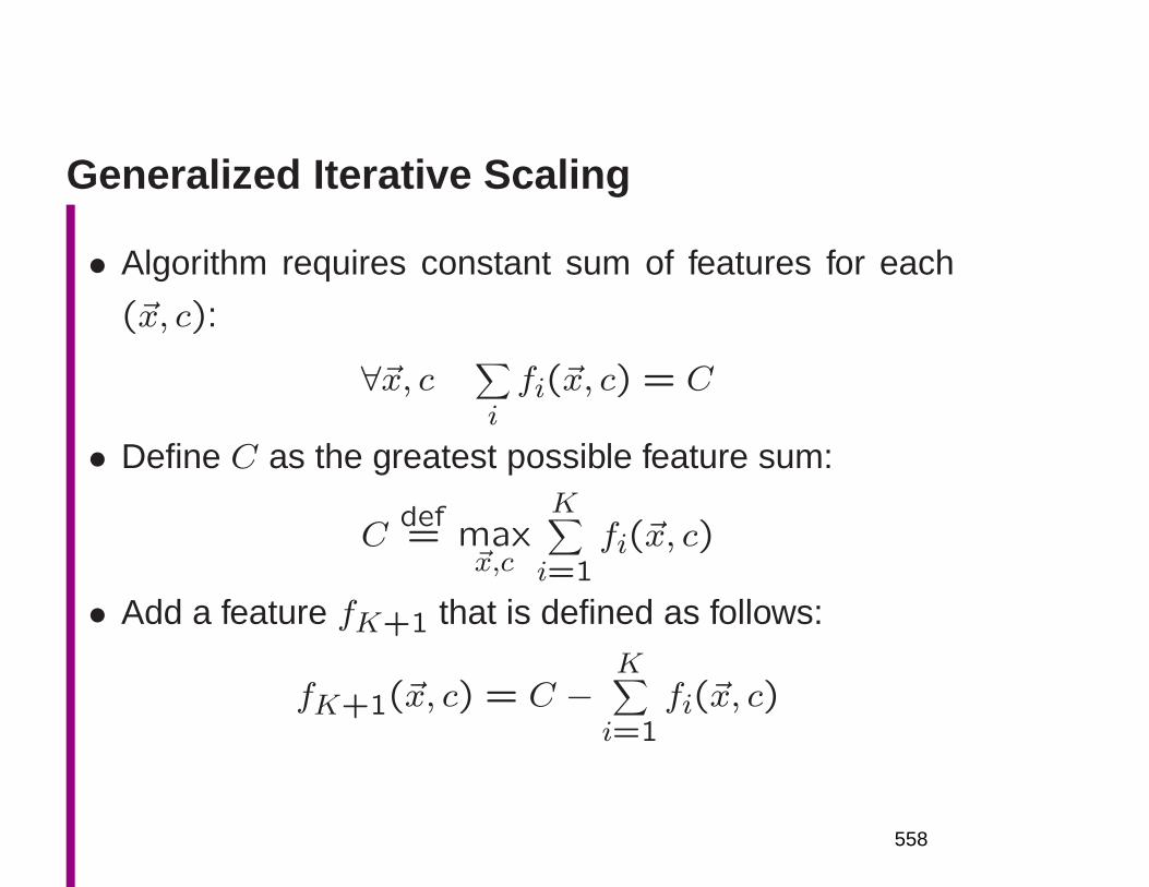
Generalized Iterative Scaling
• Algorithm requires constant sum of features for each
(~x, c):
∀~x, c ∑
ifi(~x, c) = C
• Define C as the greatest possible feature sum:
Cdef= max
~x,c
K∑
i=1fi(~x, c)
• Add a feature fK+1 that is defined as follows:
fK+1(~x, c) = C −K∑
i=1fi(~x, c)
558
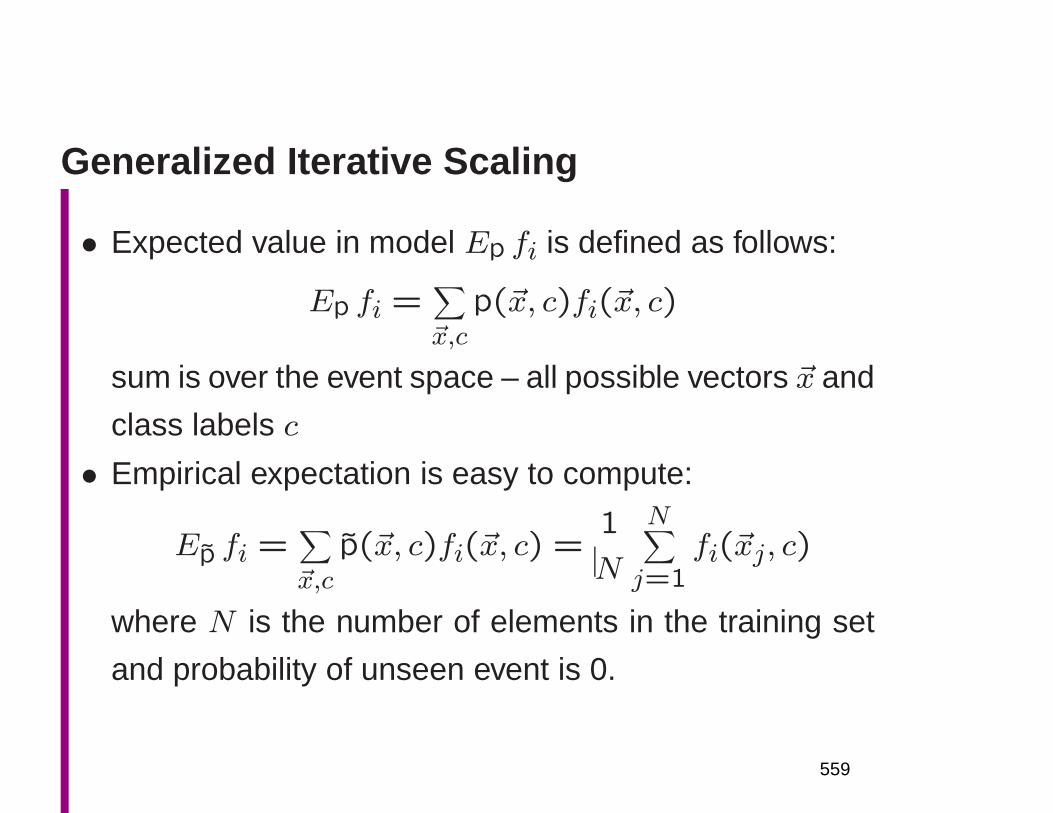
Generalized Iterative Scaling
• Expected value in model Ep fi is defined as follows:
Ep fi =∑
~x,c
p(~x, c)fi(~x, c)
sum is over the event space – all possible vectors ~x and
class labels c
• Empirical expectation is easy to compute:
Ep fi =∑
~x,c
p(~x, c)fi(~x, c) =1
N
N∑
j=1fi(~xj, c)
where N is the number of elements in the training set
and probability of unseen event is 0.
559
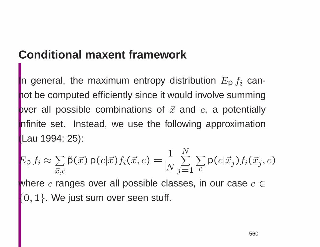
Conditional maxent framework
In general, the maximum entropy distribution Ep fi can-
not be computed efficiently since it would involve summing
over all possible combinations of ~x and c, a potentially
infinite set. Instead, we use the following approximation
(Lau 1994: 25):
Ep fi ≈∑
~x,c
p(~x) p(c|~x)fi(~x, c) =1
N
N∑
j=1
∑
cp(c|~xj)fi(~xj, c)
where c ranges over all possible classes, in our case c ∈0,1. We just sum over seen stuff.
560
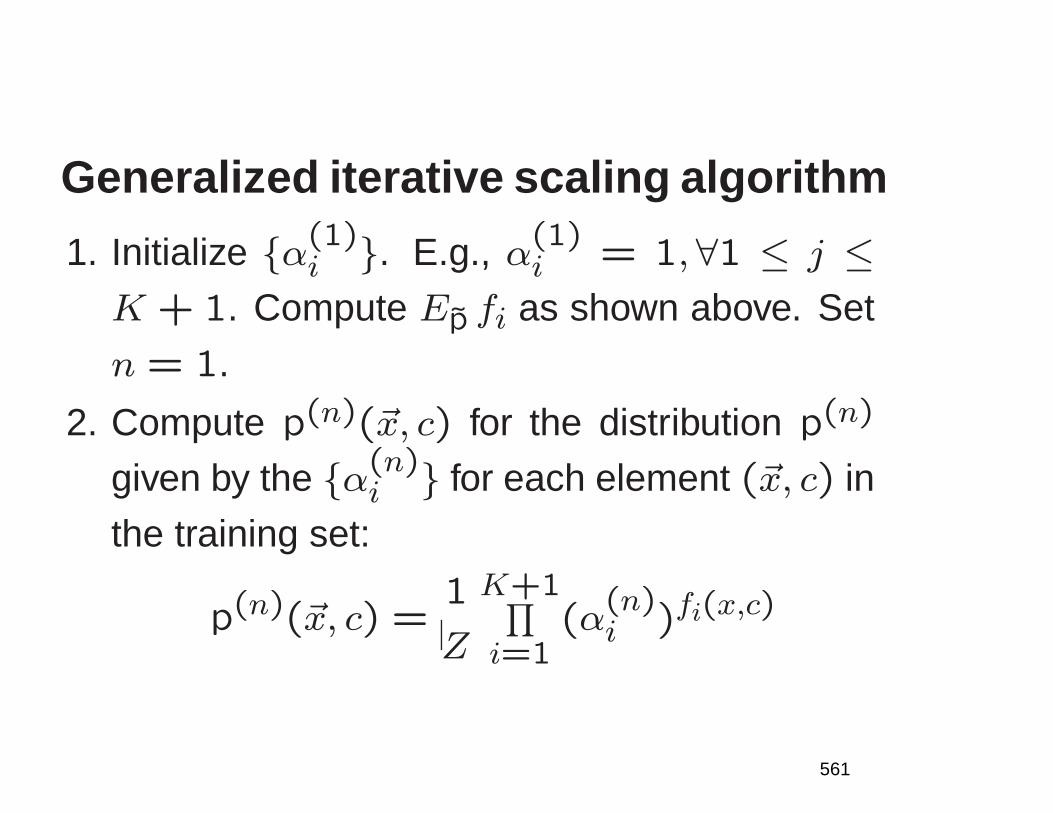
Generalized iterative scaling algorithm
1. Initialize α(1)i . E.g., α(1)
i = 1,∀1 ≤ j ≤K + 1. Compute Ep fi as shown above. Set
n = 1.
2. Compute p(n)(~x, c) for the distribution p(n)
given by the α(n)i for each element (~x, c) in
the training set:
p(n)(~x, c) =1
Z
K+1∏
i=1(α
(n)i )fi(x,c)
561
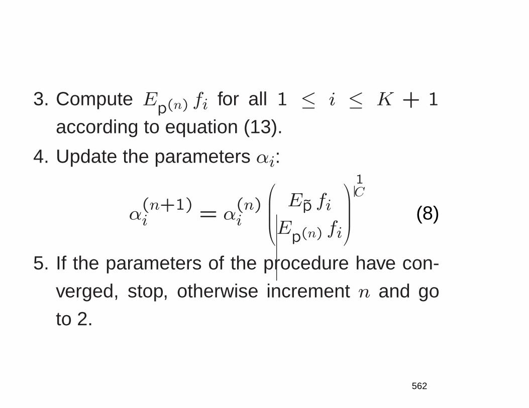
3. Compute Ep(n) fi for all 1 ≤ i ≤ K + 1
according to equation (13).
4. Update the parameters αi:
α(n+1)i = α
(n)i
Ep fiE
p(n) fi
1C
(8)
5. If the parameters of the procedure have con-
verged, stop, otherwise increment n and go
to 2.
562
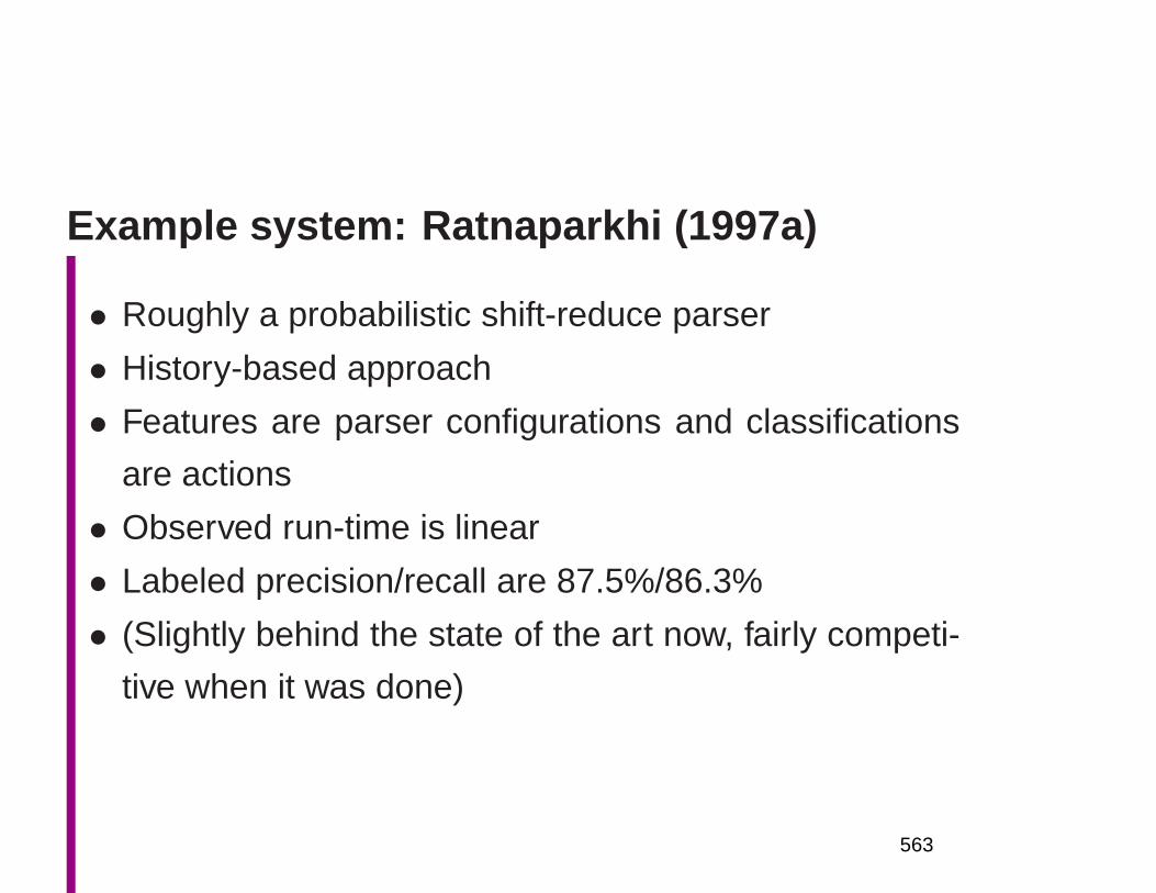
Example system: Ratnaparkhi (1997a)
• Roughly a probabilistic shift-reduce parser
• History-based approach
• Features are parser configurations and classifications
are actions
• Observed run-time is linear
• Labeled precision/recall are 87.5%/86.3%
• (Slightly behind the state of the art now, fairly competi-
tive when it was done)
563
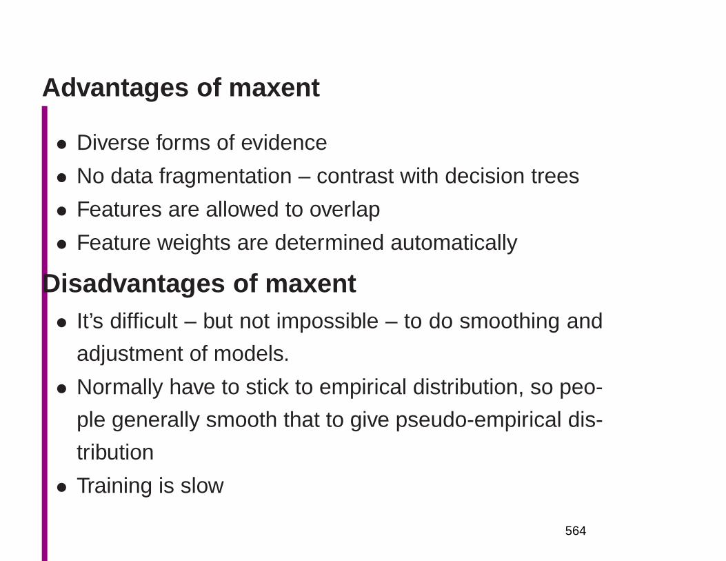
Advantages of maxent
• Diverse forms of evidence
• No data fragmentation – contrast with decision trees
• Features are allowed to overlap
• Feature weights are determined automatically
Disadvantages of maxent• It’s difficult – but not impossible – to do smoothing and
adjustment of models.
• Normally have to stick to empirical distribution, so peo-
ple generally smooth that to give pseudo-empirical dis-
tribution
• Training is slow
564
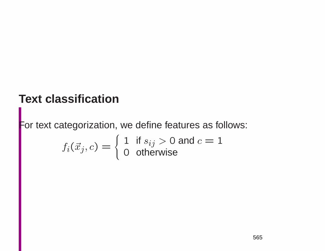
Text classification
For text categorization, we define features as follows:
fi(~xj, c) =
1 if sij > 0 and c = 10 otherwise
565

Maximum Entropy text classification
• Nigam, Lafferty, and McCallum (1999 IJCAI WS)
• Features are scaled word occurrence counts in docu-
ments
• Simple model suffered from overfitting; use Gaussian
prior, and do MAP estimation
• One can easily add bigrams, phrases (but they didn’t)
• For WebKB data, they give an error rate of 8.1%, as
against 13.7% for Naive Bayes.
• But NB was able to beat MaxEnt (by 0.7%) on a set of
newsgroup data
566

•
567
Bibliography
Baker, James K. 1979. Trainable grammars for speech recognition. InD. H. Klatt and J. J. Wolf (eds.), Speech Communication Papers for the97th Meeting of the Acoustical Society of America, pp. 547–550.
Baum, L. E., T. Petrie, G. Soules, and N. Weiss. 1970. A maximizationtechnique occurring in the statistical analysis of probabilistic functionsof Markov chains. Annals of Mathematical Statistics 41:164–171.
Bod, Rens. 1998. Beyond Grammar: An experience-based theory oflanguage. Stanford, CA: CSLI Publications.
Bod, Rens. 2000. Parsing with the shortest derivation. In COLING 18.
Borkar, Vinayak, Kaustubh Deshmukh, and Sunita Sarawagi. 2001.Automatic segmentation of text into structured records. In SIGMOD2001, pp. 175–186.
Brants, Thorsten. 2000. TnT – a statistical part-of-speech tagger. InANLP 6, pp. 224–231.
568
1
Breiman, L., and J. H. Friedman. 1988. Discussion on article byLoh and Vanichsetakul: ‘tree-structured classification via generalizeddiscriminant analysis’. Journal of the American Statistical Association83:715–727.
Breiman, L., J. H. Friedman, R. A. Olshen, and C. J. Stone. 1984.Classification and Regression Trees. Belmont, CA: Wadsworth Inter-national Group.
Brown, Peter F., Stephen A. Della Pietra, Vincent J. Della Pietra, andRobert L. Mercer. 1991a. A statistical approach to sense disambigua-tion in machine translation. In Proceedings of the DARPA Workshopon Speech and Natural Language Workshop, pp. 146–151.
Brown, Peter F., Stephen A. Della Pietra, Vincent J. Della Pietra, andRobert L. Mercer. 1991b. Word-sense disambiguation using statisticalmethods. In ACL 29, pp. 264–270.
Bruce, Rebecca, and Janyce Wiebe. 1994. Word-sense disambigua-tion using decomposable models. In ACL 32, pp. 139–145.
2
Bruce, Rebecca F., and Janyce M. Wiebe. 1999. Decomposablemodeling in natural language processing. Computational Linguistics25:195–208.
Cardie, Claire. 1993. Using decision trees to improve case-basedlearning. In Proceedings of the Tenth International Conference onMachine Learning, pp. 25–32.
Charniak, Eugene. 1993. Statistical Language Learning. Cambridge,MA: MIT Press.
Charniak, Eugene. 1996. Tree-bank grammars. In Proceedings of theThirteenth National Conference on Artificial Intelligence (AAAI ’96), pp.1031–1036.
Charniak, Eugene. 1997. Statistical parsing with a context-free gram-mar and word statistics. In Proceedings of the Fourteenth NationalConference on Artificial Intelligence (AAAI ’97), pp. 598–603.
Charniak, Eugene. 2000. A maximum-entropy-inspired parser. InNAACL 1, pp. 132–139.
3
Charniak, Eugene. 2001. Immediate-head parsing for language mod-els. In ACL 39, pp. 116–123.
Charniak, Eugene, and Mark Johnson. 2005. Coarse-to-fine n-bestparsing and maxent discriminative reranking. In ACL 43, pp. 173–180.
Chelba, Ciprian, and Frederick Jelinek. 1998. Exploiting syntacticstructure for language modeling. In ACL 36/COLING 17, pp. 225–231.
Chen, Stanley F., and Joshua Goodman. 1998. An empirical studyof smoothing techniques for language modeling. Technical ReportTR-10-98, Center for Research in Computing Technology, HarvardUniversity.
Church, Kenneth W., and William A. Gale. 1991. A comparison of theenhanced Good-Turing and deleted estimation methods for estimatingprobabilities of English bigrams. Computer Speech and Language 5:19–54.
Collins, Michael John. 1996. A new statistical parser based on bigramlexical dependencies. In ACL 34, pp. 184–191.
4
Collins, Michael John. 1997. Three generative, lexicalised models forstatistical parsing. In ACL 35/EACL 8, pp. 16–23.Collins, Michael John, and James Brooks. 1995. Prepositional phraseattachment through a backed-off model. In WVLC 3, pp. 27–38.Cover, Thomas M., and Joy A. Thomas. 1991. Elements of InformationTheory. New York: John Wiley & Sons.Daelemans, Walter, Jakub Zavrel, Peter Berck, and Steven Gillis.1996. MBT: A memory-based part of speech tagger generator. InWVLC 4, pp. 14–27.Dagan, Ido, and Alon Itai. 1994. Word sense disambiguation using asecond language monolingual corpus. Computational Linguistics 20:563–596.Dagan, Ido, Lillian Lee, and Fernando Pereira. 1999. Similarity-basedmodels of word co-occurrence probabilities. Machine Learning 34:43–69.Dempster, A.P., N.M. Laird, and D.B. Rubin. 1977. Maximum likelihoodfrom incomplete data via the EM algorithm. J. Royal Statistical SocietySeries B 39:1–38.
5
Domingos, Pedro, and Michael Pazzani. 1997. On the optimality of thesimple Bayesian classifier under zero-one loss. Machine Learning 29:103–130.Duda, Richard O., and Peter E. Hart. 1973. Pattern classification andscene analysis. New York: Wiley.Ford, Marilyn, Joan Bresnan, and Ronald M. Kaplan. 1982. Acompetence-based theory of syntactic closure. In Joan Bresnan (ed.),The Mental Representation of Grammatical Relations, pp. 727–796.Cambridge, MA: MIT Press.Franz, Alexander. 1997. Independence assumptions considered harm-ful. In ACL 35/EACL 8, pp. 182–189.Freitag, Dayne, and Andrew McCallum. 1999. Information extractionwith HMMs and shrinkage. In AAAI ’99 Workshop on Machine Learningfor Information Extraction, pp. 31–36.Freitag, Dayne, and Andrew McCallum. 2000. Information extractionwith HMM structures learned by stochastic optimization. In Proceed-ings of AAAI, pp. 584–589.
6
Friedman, Jerome H. 1997. On bias, variance, 0/1–loss, and the curse-of-dimensionality. Data Mining and Knowledge Discovery 1:55–77.Friedman, Nir, and M. Goldszmidt. 1996. Building classifiers usingBayesian networks. In AAAI ’96, pp. 1277–1284.Gale, William A., Kenneth W. Church, and David Yarowsky. 1992. Amethod for disambiguating word senses in a large corpus. Computersand the Humanities 26:415–439.Gale, William A., and Geoffrey Sampson. 1995. Good-Turing fre-quency estimation without tears. Journal of Quantitative Linguistics 2:217–237.Gold, E. Mark. 1967. Language identification in the limit. Informationand Control 10:447–474.Goodman, Joshua. 2001. A bit of progress in language modeling,extended version. Technical Report MSR-TR-2001-72, Microsoft Re-search.Hindle, Donald, and Mats Rooth. 1993. Structural ambiguity and lexicalrelations. Computational Linguistics 19:103–120.
7
Horning, James Jay. 1969. A study of grammatical inference. PhDthesis, Stanford.Johnson, Mark. 1998a. The effect of alternative tree representa-tions on tree bank grammars. In Proceedings of Joint Conferenceon New Methods in Language Processing and Computational Natu-ral Language Learning (NeMLaP3/CoNLL98), pp. 39–48, MacquarieUniversity.Johnson, Mark. 1998b. PCFG models of linguistic tree representa-tions. Computational Linguistics 24:613–632.Katz, Slava M. 1987. Estimation of probabilities from sparse datafor the language model component of a speech recognizer. IEEETransactions on Acoustics, Speech, and Signal Processing ASSP-35:400–401.Kilgarriff, Adam. 1997. “I don’t believe in word senses”. Computersand the Humanities 31:91–113.Klein, Dan, and Christopher D. Manning. 2003. Accurate unlexicalizedparsing. In ACL 41, pp. 423–430.
8
Kneser, Reinhard, and Hermann Ney. 1995. Improved backing-off form-gram language modeling. In Proceedings of the IEEE Conferenceon Acoustics, Speech and Signal Processing, volume 1, pp. 181–184.
Koller, Daphne, and Mehran Sahami. 1996. Toward optimal featureselection. In ICML ’96, pp. 284–292.
Kupiec, Julian. 1992. Robust part-of-speech tagging using a HiddenMarkov Model. Computer Speech and Language 6:225–242.
Laplace, Pierre Simon marquis de. 1814. Essai philosophique sur lesprobabilites. Paris: Mme. Ve. Courcier.
Lari, K., and S. J. Young. 1990. The estimation of stochastic context-free grammars using the inside-outside algorithm. Computer Speechand Language 4:35–56.
Lau, Raymond. 1994. Adaptive statistical language modelling. Mas-ter’s thesis, Massachusetts Institute of Technology.
Lesk, Michael. 1986. Automatic sense disambiguation: How to tella pine cone from an ice cream cone. In Proceedings of the 1986
9
SIGDOC Conference, pp. 24–26, New York. Association for ComputingMachinery.
Magerman, David M. 1995. Statistical decision-tree models for pars-ing. In ACL 33, pp. 276–283.
Manning, Christopher D., and Bob Carpenter. 1997. Probabilisticparsing using left corner language models. In Proceedings of the FifthInternational Workshop on Parsing Technologies (IWPT-97), pp. 147–158, MIT.
Manning, Christopher D., and Hinrich Schütze. 1999. Foundations ofStatistical Natural Language Processing. Boston, MA: MIT Press.
Marcus, Mitchell P., Beatrice Santorini, and Mary Ann Marcinkiewicz.1993. Building a large annotated corpus of English: The Penn tree-bank. Computational Linguistics 19:313–330.
McCallum, Andrew, and Kamal Nigam. 1998. A comparison of eventmodels for naive bayes text classification. In Working Notes of the 1998AAAI/ICML Workshop on Learning for Text Categorization, pp. 41–48.
10
McLachlan, Geoffrey J., and Thiriyambakam Krishnan. 1996. The EMAlgorithm and Extensions. John Wiley & Sons.Merlo, Paola, Matthew Crocker, and Cathy Berthouzoz. 1997. Attach-ing multiple prepositional phrases: Generalized backed-off estimation.In EMNLP 2, pp. 149–155.Mitchell, Tom M. (ed.). 1997. Machine Learning. New York: McGraw-Hill.Ney, Hermann, Sven Martin, and Frank Wessel. 1997. Statisticallanguage modeling using leaving-one-out. In Steve Young and GerritBloothooft (eds.), Corpus-Based Methods in Language and SpeechProcessing, pp. 174–207. Dordrecht: Kluwer Academic.Pasca, Marius, and Sanda Harabagiu. 2001. High performance ques-tion/answering. In SIGIR ’01, pp. 366–374.Quinlan, J. R. 1986. Induction of decision trees. Machine Learning 1:81–106. Reprinted in (Shavlik and Dietterich 1990).Ratnaparkhi, Adwait. 1997a. A linear observed time statistical parserbased on maximum entropy models. In EMNLP 2, pp. 1–10.
11
Ratnaparkhi, Adwait. 1997b. A simple introduction to maximum en-tropy models for natural language processing. Technical Report IRCSReport 97–08, Institute for Research in Cognitive Science, Philadel-phia, PA.Ratnaparkhi, Adwait. 1998. Unsupervised statistical models for prepo-sitional phrase attachment. In ACL 36/COLING 17, pp. 1079–1085.Ratnaparkhi, Adwait. 1999. Learning to parse natural language withmaximum entropy models. Machine Learning 34:151–175.Ripley, B. D. 1996. Pattern Recognition and Neural Networks. Cam-bridge: Cambridge University Press.Rosenfeld, Ronald. 1996. A maximum entropy approach to adaptivestatistical language modeling. Computer, Speech and Language 10:187–228.Rosenfeld, Ronald. 2000. Two decades of statistical language model-ing: Where do we go from here? Proceedings of the IEEE 88.Schütze, Hinrich. 1998. Automatic word sense discrimination. Com-putational Linguistics 24:97–124.
12
Shavlik, Jude W., and Thomas G. Dietterich (eds.). 1990. Readings inMachine Learning. San Mateo, CA: Morgan Kaufmann.
Toutanova, Kristina, Dan Klein, Christopher D. Manning, and YoramSinger. 2003. Feature-rich part-of-speech tagging with a cyclic depen-dency network. In NAACL 3, pp. 252–259.
van Rijsbergen, C. J. 1979. Information Retrieval. London: Butter-worths. Second Edition.
Viterbi, A. J. 1967. Error bounds for convolutional codes and anasymptotically optimum decoding algorithm. IEEE Transactions onInformation Theory IT-13:260–269.
Yarowsky, David. 1992. Word-sense disambiguation using statisticalmodels of Roget’s categories trained on large corpora. In COLING 14,pp. 454–460.
Yarowsky, David. 1995. Unsupervised word sense disambiguationrivaling supervised methods. In ACL 33, pp. 189–196.