Introduction K R - palmer.wellesley.edupalmer.wellesley.edu/~ivolic/pdf/Papers/ThesisPaperMaster2.pdf · There are canonical maps K→Hr and Hr →Hr−1, ... The sign convention

FINITE TYPE KNOT INVARIANTS AND CALCULUS OF FUNCTORS

ISMAR VOLIC

Abstract. We associate a Taylor tower supplied by calculus of the embedding functor to thespace of long knots and study its cohomology spectral sequence. The combinatorics of the spectralsequence along the line of total degree zero leads to chord diagrams with relations as in finite typeknot theory. We show that the spectral sequence collapses along this line and that the Taylortower represents a universal finite type knot invariant.

1. Introduction

In this paper we bring together two fields, finite type knot theory and Goodwillie’s calculus offunctors, both of which have received considerable attention during the past ten years. Goodwillieand his collaborators have known for some time, through their study of the embedding functor,that there should be a strong connection between the two [17, 18]. This is indeed the case, andwe will show that a certain tower of spaces in the calculus of embeddings serves as a classifyingobject for finite type knot invariants.

Let K be the space of framed long knots, i.e. embeddings of R into R3 which agree with some

fixed linear inclusion of R into R3 outside a compact set, and come equipped with a choice of a

nowhere-vanishing section of the normal bundle. Alternatively, we may think of K as the space offramed based knots in S3, namely framed maps of the unit interval I to S3 which are embeddingsexcept at the endpoints. The endpoints are mapped to some basepoint in S3 with the samederivative. It is not hard to see that these two versions of K are homotopy equivalent.

Now consider (framed) singular long knots which are (framed) long knots with a finite numberof transverse double points. We can extend any knot invariant V to such knots by applying it toall knots obtained by resolving the double points of a singular knot in two possible ways, withappropriate signs. If V vanishes on knots with more than n double points, then it is of type n.

As will be explained in more detail in §2, it turns out that Vn, the set of all type n invariants, isclosely related to the space generated by chord diagrams with n chords modulo a certain relation.In fact, if Wn denotes the dual of this space, then Kontsevich [21] proves

Theorem 1.1. Vn/Vn−1∼=Wn.

An alternative proof of this theorem uses Bott-Taubes configuration space integrals which play acrucial role in the proofs of our results. These are briefly described in §3, but more details canbe found in [5, 31].

The other ingredient we need is the Taylor tower for K defined in some detail in §4. Followingwork of Weiss [32], one can construct spaces Hr for each r > 1, defined as homotopy limits of

1991 Mathematics Subject Classification. Primary: 57R40; Secondary: 57M27, 57T35.Key words and phrases. calculus of functors, finite type invariants, Vassiliev invariants, knots, spaces of knots,

configuration spaces.

1

2 ISMAR VOLIC

certain diagrams of “punctured knots,” namely embeddings of I in S3 as before but with somenumber of subintervals removed. There are canonical maps K → Hr and Hr → Hr−1, and thesecombine to yield the Taylor tower.

To study the tower, we introduce in §5 a cosimplicial space X• whose rth partial totalization isprecisely the stage Hr (Theorem 5.6). This equivalence was shown by Sinha [28]. The advantageof the cosimplicial point of view is that X• comes equipped with a (second quadrant) cohomologyspectral sequence. This spectral sequence computes the cohomology of the total complex T ∗r of thedouble complex obtained by applying cochains to the truncated cosimplicial space. Alternatively,one can pass to real linear combinations generated by the spaces in the cosimplicial space andtake the rth partial totalization to get T ∗r again. It is the latter description of this algebraicanalog of the Taylor tower that we use for our proofs (see §6.3 for exact description of the stagesT ∗r ), because sums of resolutions of singular knots can be mapped into such a tower. We can nowstate the main result:

Theorem 1.2. H0(T ∗2n) ∼= Vn.

Moreover, all finite type invariants factor through the algebraic Taylor tower for K, as the aboveisomorphism is induced by a map which is essentially a collection of evaluation maps (see Propo-sition 5.5). Unfortunately, it is not known that the algebraic stages and ordinary stages of theTaylor tower have the same homology, although this is believed to be the case (Sinha [28] hasshown this for any space of embeddings of one manifold in another, as long as the codimensionis at least 3).

The starting point in the proof of the above theorem is Proposition 6.2, which states thatthe groups on the diagonal of the E1 term of the spectral sequence can be associated to chorddiagrams. We then show

• E−2n,2n∞

∼= H0(T ∗2n)/H0(T ∗2n−1) (§6.2),

• E−2n,2n2

∼=Wn (Proposition 6.3),• There is a commutative diagram

E−2n,2n∞

// _

Vn/Vn−1 _

E−2n,2n

2

∼= // Wn

(Proposition 6.4).

The proof of the second statement is a direct computation of the first differential in the spectralsequence. The other parts follow from considering how a singular knot maps into the algebraicTaylor tower.

We then use Theorem 4.2 to finish the proofs in §6.4. This theorem essentially states that Bott-Taubes integration fits as a diagonal map from Wn to E−2n,2n

∞ in the above square and makesthe top resulting triangle commute. It follows that all the maps in the diagram are isomorphismsover the rationals (Bott-Taubes integrals are the only reason we cannot state our results over theintegers). In addition to deducing Theorem 1.2, we also have an alternative proof of Theorem 1.1,as well as

Theorem 1.3. The spectral sequence collapses on the diagonal at E2.

FINITE TYPE KNOT INVARIANTS AND CALCULUS OF FUNCTORS 3

Thus calculus of the embedding functor provides a new point of view on finite type knot theory.Some further questions as well as a brief discussion of the potential importance of this point ofview can be found in §6.5.

1.1. Acknowledgements. I am deeply endebted to my thesis advisor, Tom Goodwillie, whoseknowledge is only matched by his desire to share it. Dev Sinha’s help over the years has alsobeen invaluable. I am thankful to Pascal Lambrechts and Greg Arone for many comments andsuggestions.

2. Finite type knot invariants

Here we recall some basic features of finite type knot theory. More details can be found in[3, 4].

As mentioned earlier, a singular long knot is a long knot except for a finite number of doublepoints. The tangent vectors at the double points are required to be independent. A knot with nsuch self-intersections is called n-singular.

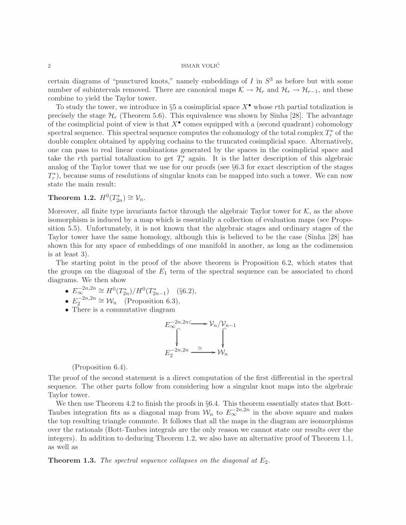
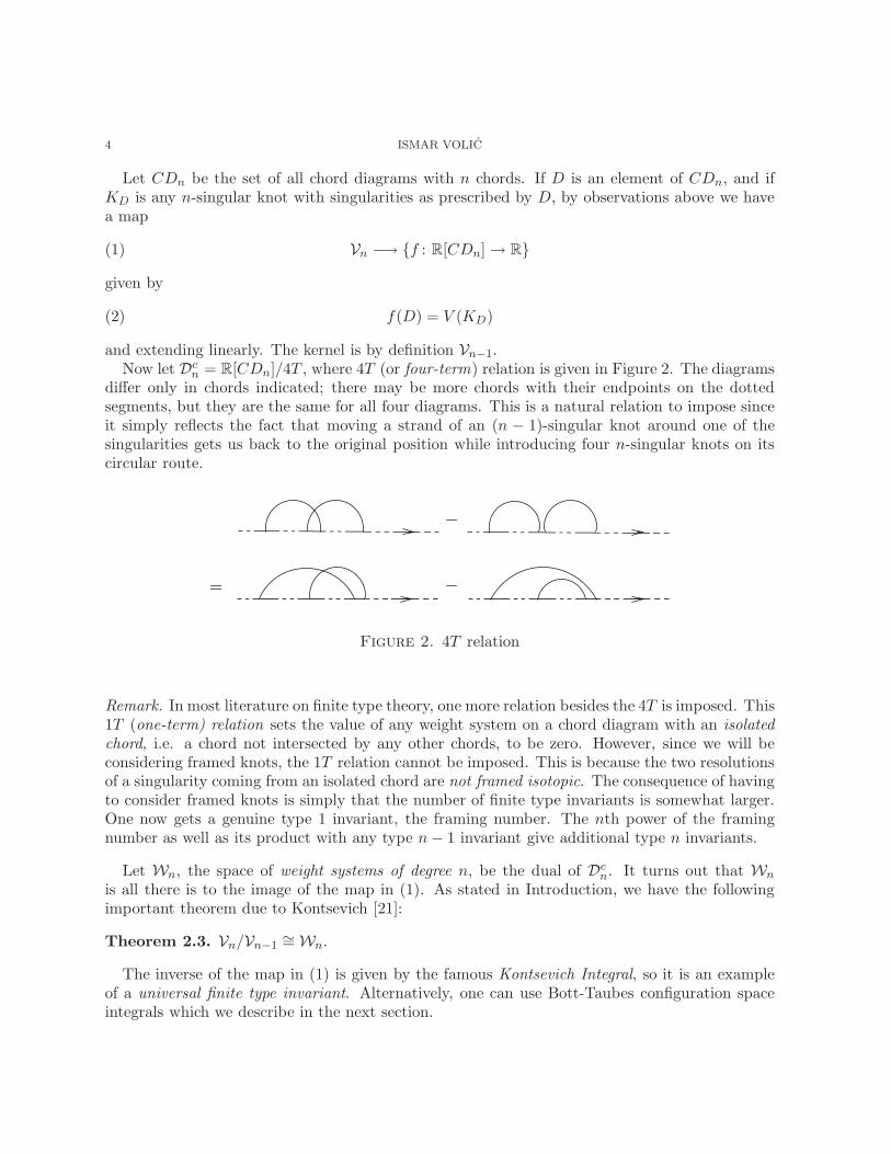
One can now use the Vassiliev skein relation, pictured in Figure 1, to extend any knot invariantV to singular knots.

)− V

()= V

( )V

(

Figure 1. Vassiliev skein relation

The drawings mean that the three knots only differ locally in one crossing. A n-singular knotthus produces 2n resolutions. The sign convention ensures that the order in which we resolve thesingularities does not matter.

Definition 2.1. V is a (finite, or Vassiliev) type n invariant if it vanishes identically on singularknots with n + 1 self-intersections.

Let V be the collection of all finite type invariants and let Vn be the set of type n invariants. Itis easy to see, for example, that V0 and V1 (for unframed knots) both contain only the constantfunctions on K. Also immediate is that Vn contains Vn−1.

Another quick consequence of the definition is that the value of a type n invariant on an n-singular knot only depends on the placement of its singularities. This is because if two n-singularknots differ only in the embedding, the difference of V ∈ Vn evaluated on one and the other isthe value of V on some (n + 1)-singular knots (since one can get from one knot to the other by asequence of crossing changes). But V by definition vanishes on such knots.

It thus follows that the value of V on n-singular knots is closely related to the following objects:

Definition 2.2. A chord diagram of degree n is an oriented interval with 2n paired-off points onit, regarded up to orientation-preserving diffeomorphisms of the interval.

The pairs of points can be thought of as prescriptions for where the singularities on the knotshould occur, while how the rest of the interval is embedded is immaterial.

4 ISMAR VOLIC

Let CDn be the set of all chord diagrams with n chords. If D is an element of CDn, and ifKD is any n-singular knot with singularities as prescribed by D, by observations above we havea map

(1) Vn −→ f : R[CDn]→ R

given by

(2) f(D) = V (KD)

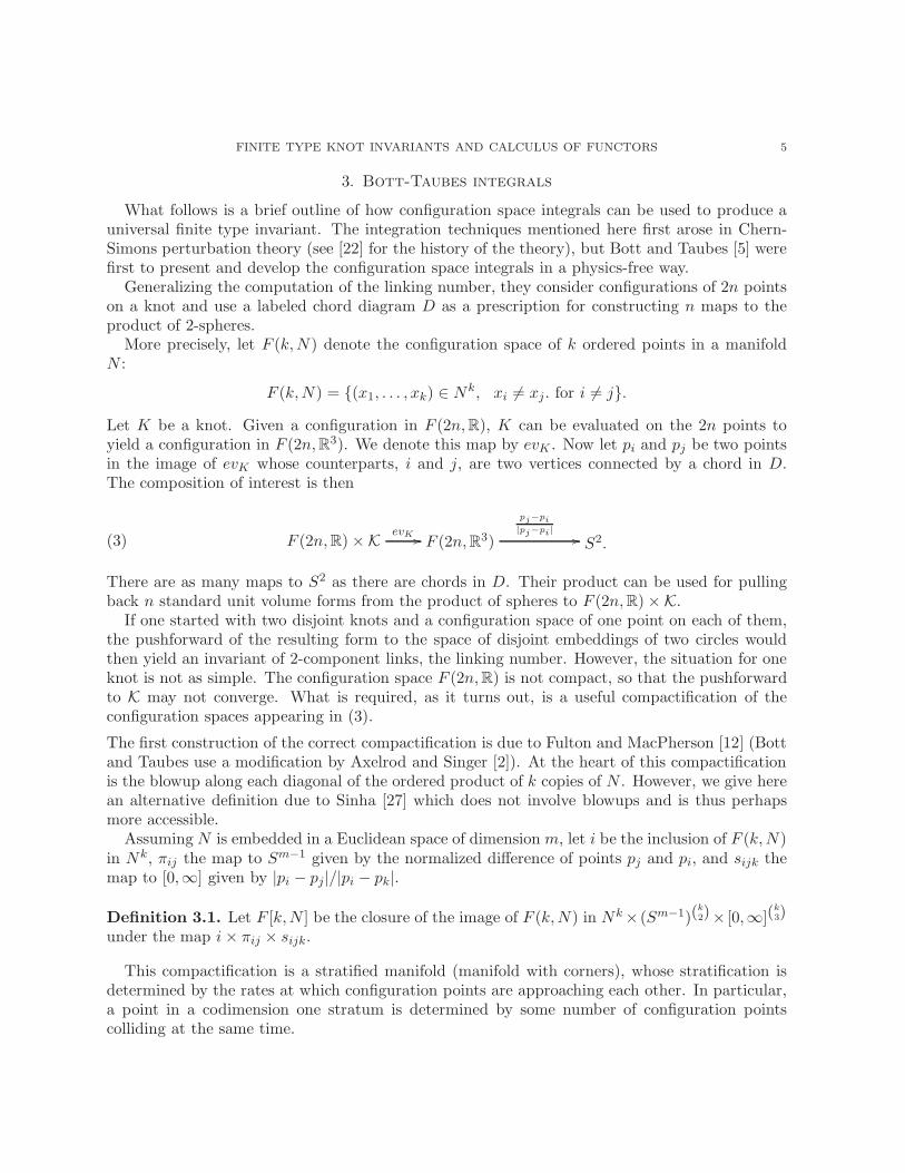
and extending linearly. The kernel is by definition Vn−1.Now let Dc

n = R[CDn]/4T , where 4T (or four-term) relation is given in Figure 2. The diagramsdiffer only in chords indicated; there may be more chords with their endpoints on the dottedsegments, but they are the same for all four diagrams. This is a natural relation to impose sinceit simply reflects the fact that moving a strand of an (n − 1)-singular knot around one of thesingularities gets us back to the original position while introducing four n-singular knots on itscircular route.

−

−=

Figure 2. 4T relation

Remark. In most literature on finite type theory, one more relation besides the 4T is imposed. This1T (one-term) relation sets the value of any weight system on a chord diagram with an isolatedchord, i.e. a chord not intersected by any other chords, to be zero. However, since we will beconsidering framed knots, the 1T relation cannot be imposed. This is because the two resolutionsof a singularity coming from an isolated chord are not framed isotopic. The consequence of havingto consider framed knots is simply that the number of finite type invariants is somewhat larger.One now gets a genuine type 1 invariant, the framing number. The nth power of the framingnumber as well as its product with any type n− 1 invariant give additional type n invariants.

Let Wn, the space of weight systems of degree n, be the dual of Dcn. It turns out that Wn

is all there is to the image of the map in (1). As stated in Introduction, we have the followingimportant theorem due to Kontsevich [21]:


The inverse of the map in (1) is given by the famous Kontsevich Integral, so it is an exampleof a universal finite type invariant. Alternatively, one can use Bott-Taubes configuration spaceintegrals which we describe in the next section.


3. Bott-Taubes integrals

What follows is a brief outline of how configuration space integrals can be used to produce auniversal finite type invariant. The integration techniques mentioned here first arose in Chern-Simons perturbation theory (see [22] for the history of the theory), but Bott and Taubes [5] werefirst to present and develop the configuration space integrals in a physics-free way.

Generalizing the computation of the linking number, they consider configurations of 2n pointson a knot and use a labeled chord diagram D as a prescription for constructing n maps to theproduct of 2-spheres.

More precisely, let F (k,N) denote the configuration space of k ordered points in a manifoldN :

F (k,N) = (x1, . . . , xk) ∈ Nk, xi 6= xj. for i 6= j.

Let K be a knot. Given a configuration in F (2n, R), K can be evaluated on the 2n points toyield a configuration in F (2n, R3). We denote this map by evK . Now let pi and pj be two pointsin the image of evK whose counterparts, i and j, are two vertices connected by a chord in D.The composition of interest is then

(3) F (2n, R)×KevK // F (2n, R3)

pj−pi

|pj−pi| // S2.

There are as many maps to S2 as there are chords in D. Their product can be used for pullingback n standard unit volume forms from the product of spheres to F (2n, R)×K.

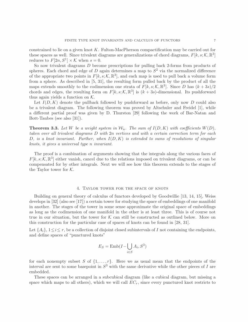
If one started with two disjoint knots and a configuration space of one point on each of them,the pushforward of the resulting form to the space of disjoint embeddings of two circles wouldthen yield an invariant of 2-component links, the linking number. However, the situation for oneknot is not as simple. The configuration space F (2n, R) is not compact, so that the pushforwardto K may not converge. What is required, as it turns out, is a useful compactification of theconfiguration spaces appearing in (3).

The first construction of the correct compactification is due to Fulton and MacPherson [12] (Bottand Taubes use a modification by Axelrod and Singer [2]). At the heart of this compactificationis the blowup along each diagonal of the ordered product of k copies of N . However, we give herean alternative definition due to Sinha [27] which does not involve blowups and is thus perhapsmore accessible.

Assuming N is embedded in a Euclidean space of dimension m, let i be the inclusion of F (k,N)in Nk, πij the map to Sm−1 given by the normalized difference of points pj and pi, and sijk themap to [0,∞] given by |pi − pj|/|pi − pk|.

Definition 3.1. Let F [k,N ] be the closure of the image of F (k,N) in Nk× (Sm−1)(k2)× [0,∞](

k3)

under the map i× πij × sijk.

This compactification is a stratified manifold (manifold with corners), whose stratification isdetermined by the rates at which configuration points are approaching each other. In particular,a point in a codimension one stratum is determined by some number of configuration pointscolliding at the same time.

6 ISMAR VOLIC

The most useful feature of this construction is that the directions of approach of the collidingpoints are kept track of. This allows Bott and Taubes to rewrite (3) as

(4) F [2n, R]×K −→ F [2n, R3] −→ S2

and they show that the product of the 2-forms which are pulled back from the spheres extendssmoothly to the boundary of F [2n, R] (for details, also see [31]). The advantage is that now onecan produce a function on the space of knots K by integrating the resulting 2n-form along thecompact fiber F [2n, R] of the projection

π : F [2n, R]×K −→ K.

More precisely, let ω be the product of the volume forms on (S2)n and let hD be the product ofthe compositions in (4). What has just been described is a function on K, which we denote byI(D,K), given by

(5) I(D,K) = π∗(h∗Dω).

The question now is whether I(D,K) is a closed 0-form, or a knot invariant. To check this, itsuffices by Stokes’ Theorem to examine the pushforward π∗ along the codimension one faces ofF [2n, R]. If the integrals vanish on every such face, (5) yields a knot invariant.

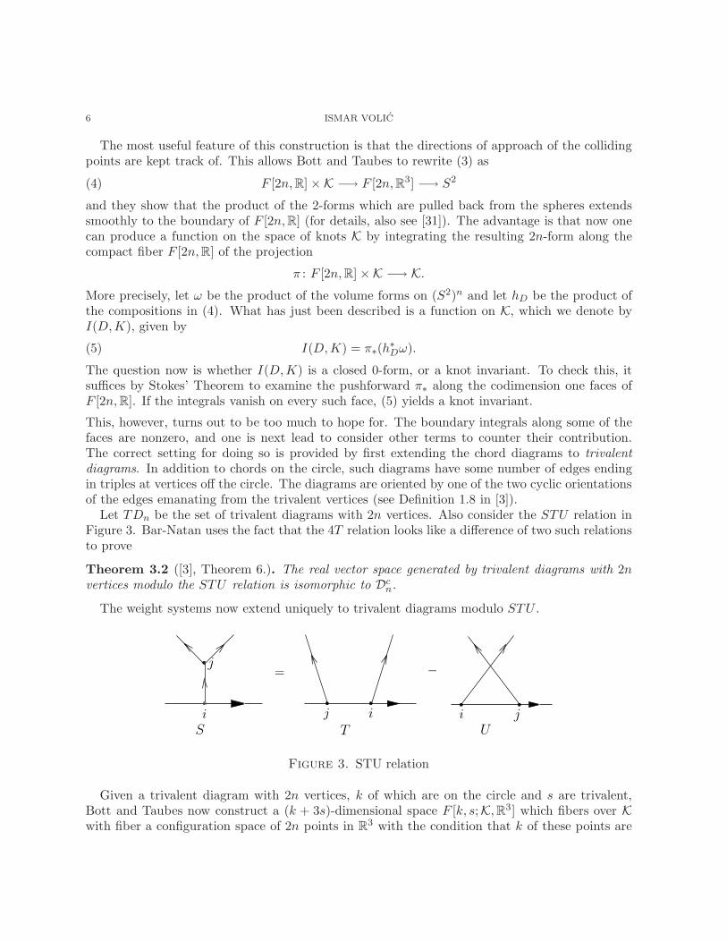
This, however, turns out to be too much to hope for. The boundary integrals along some of thefaces are nonzero, and one is next lead to consider other terms to counter their contribution.The correct setting for doing so is provided by first extending the chord diagrams to trivalentdiagrams. In addition to chords on the circle, such diagrams have some number of edges endingin triples at vertices off the circle. The diagrams are oriented by one of the two cyclic orientationsof the edges emanating from the trivalent vertices (see Definition 1.8 in [3]).

Let TDn be the set of trivalent diagrams with 2n vertices. Also consider the STU relation inFigure 3. Bar-Natan uses the fact that the 4T relation looks like a difference of two such relationsto prove

Theorem 3.2 ([3], Theorem 6.). The real vector space generated by trivalent diagrams with 2nvertices modulo the STU relation is isomorphic to Dc

n.

The weight systems now extend uniquely to trivalent diagrams modulo STU .

= −

j

j

iijiS UT

Figure 3. STU relation

Given a trivalent diagram with 2n vertices, k of which are on the circle and s are trivalent,Bott and Taubes now construct a (k + 3s)-dimensional space F [k, s;K, R3] which fibers over Kwith fiber a configuration space of 2n points in R

3 with the condition that k of these points are


constrained to lie on a given knot K. Fulton-MacPherson compactification may be carried out forthese spaces as well. Since trivalent diagrams are generalizations of chord diagrams, F [k, s;K, R3]reduces to F [2n, S1]×K when s = 0.

So now trivalent diagrams D become prescriptions for pulling back 2-forms from products ofspheres. Each chord and edge of D again determines a map to S2 via the normalized differenceof the appropriate two points in F [k, s;K, R3], and each map is used to pull back a volume formfrom a sphere. As described in [5, 31], the resulting form pulled back by the product of all themaps extends smoothly to the codimension one strata of F [k, s;K, R3]. Since D has (k + 3s)/2chords and edges, the resulting form on F [k, s;K, R3] is (k + 3s)-dimensional. Its pushforwardthus again yields a function on K.

Let I(D,K) denote the pullback followed by pushforward as before, only now D could alsobe a trivalent diagram. The following theorem was proved by Altschuler and Freidel [1], whilea different partial proof was given by D. Thurston [29] following the work of Bar-Natan andBott-Taubes (see also [31]).

Theorem 3.3. Let W be a weight system in Wn. The sum of I(D,K) with coefficients W (D),taken over all trivalent diagrams D with 2n vertices and with a certain correction term for eachD, is a knot invariant. Further, when I(D,K) is extended to sums of resolutions of singularknots, it gives a universal type n invariant.

The proof is a combination of arguments showing that the integrals along the various faces ofF [k, s;K, R3] either vanish, cancel due to the relations imposed on trivalent diagrams, or can becompensated for by other integrals. Next we will see how this theorem extends to the stages ofthe Taylor tower for K.

4. Taylor tower for the space of knots

Building on general theory of calculus of functors developed by Goodwillie [13, 14, 15], Weissdevelops in [32] (also see [17]) a certain tower for studying the space of embeddings of one manifoldin another. The stages of the tower in some sense approximate the original space of embeddingsas long as the codimension of one manifold in the other is at least three. This is of course nottrue in our situation, but the tower for K can still be constructed as outlined below. More onthis construction for the particular case of spaces of knots can be found in [28, 31].

Let Ai, 1≤ i≤ r, be a collection of disjoint closed subintervals of I not containing the endpoints,and define spaces of “punctured knots”

ES = Emb(I−⋃

i∈S

Ai, S3)

for each nonempty subset S of 1, . . . , r. Here we as usual mean that the endpoints of theinterval are sent to some basepoint in S3 with the same derivative while the other pieces of I areembedded.

These spaces can be arranged in a subcubical diagram (like a cubical diagram, but missing aspace which maps to all others), which we will call ECr, since every punctured knot restricts to

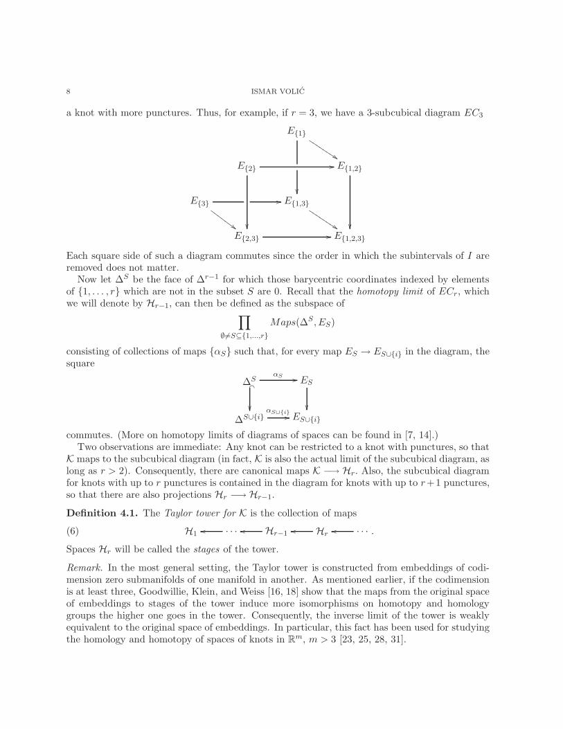
8 ISMAR VOLIC

a knot with more punctures. Thus, for example, if r = 3, we have a 3-subcubical diagram EC3

E1

$$JJ

JJ

JJ

JJ

E2 //

E1,2

E3 //

##GG

GG

GG

G

E1,3

$$JJ

JJ

JJ

JJ

E2,3 // E1,2,3

Each square side of such a diagram commutes since the order in which the subintervals of I areremoved does not matter.

Now let ∆S be the face of ∆r−1 for which those barycentric coordinates indexed by elementsof 1, . . . , r which are not in the subset S are 0. Recall that the homotopy limit of ECr, whichwe will denote by Hr−1, can then be defined as the subspace of

∏

∅6=S⊆1,...,r

Maps(∆S, ES)

consisting of collections of maps αS such that, for every map ES → ES∪i in the diagram, thesquare

∆SαS //

_

ES

∆S∪iαS∪i// ES∪i

commutes. (More on homotopy limits of diagrams of spaces can be found in [7, 14].)Two observations are immediate: Any knot can be restricted to a knot with punctures, so that

K maps to the subcubical diagram (in fact, K is also the actual limit of the subcubical diagram, aslong as r > 2). Consequently, there are canonical maps K −→ Hr. Also, the subcubical diagramfor knots with up to r punctures is contained in the diagram for knots with up to r+1 punctures,so that there are also projections Hr −→ Hr−1.

Definition 4.1. The Taylor tower for K is the collection of maps

(6) H1 · · ·oo Hr−1oo Hr

oo · · ·oo .

Spaces Hr will be called the stages of the tower.

Remark. In the most general setting, the Taylor tower is constructed from embeddings of codi-mension zero submanifolds of one manifold in another. As mentioned earlier, if the codimensionis at least three, Goodwillie, Klein, and Weiss [16, 18] show that the maps from the original spaceof embeddings to stages of the tower induce more isomorphisms on homotopy and homologygroups the higher one goes in the tower. Consequently, the inverse limit of the tower is weaklyequivalent to the original space of embeddings. In particular, this fact has been used for studyingthe homology and homotopy of spaces of knots in R

m, m > 3 [23, 25, 28, 31].


In [31], we show how Bott-Taubes integrals can be extended to the stages. We integrate overcertain spaces which generalize F [k, s;K, R3]. The k points no longer represent a configurationon a single knot, but rather on a family of punctured knots h, i.e. an element of H2n. Denotingby I(D,h) the analog of (5), we prove

Theorem 4.2. [31, Theorem 4.1] Let W be a weight system in Wn and let D be a trivalentdiagram with 2n vertices. Then the sum of I(D,h) over all D, with coefficients W (D), is aninvariant of H2n, provided a correction term is given for each D. In particular, this restricts tothe invariant of K described in Theorem 3.3 when a point in H2n comes from a knot.

The next goal is to see how our invariants T (W ) behave when singular knots, or rather sumsof their resolutions, are mapped into the stages H2n. To that end, we introduce a cosimplicialmodel for the Taylor tower because it is suitable for our computational purposes.

5. A Cosimplicial Model for the Taylor Tower

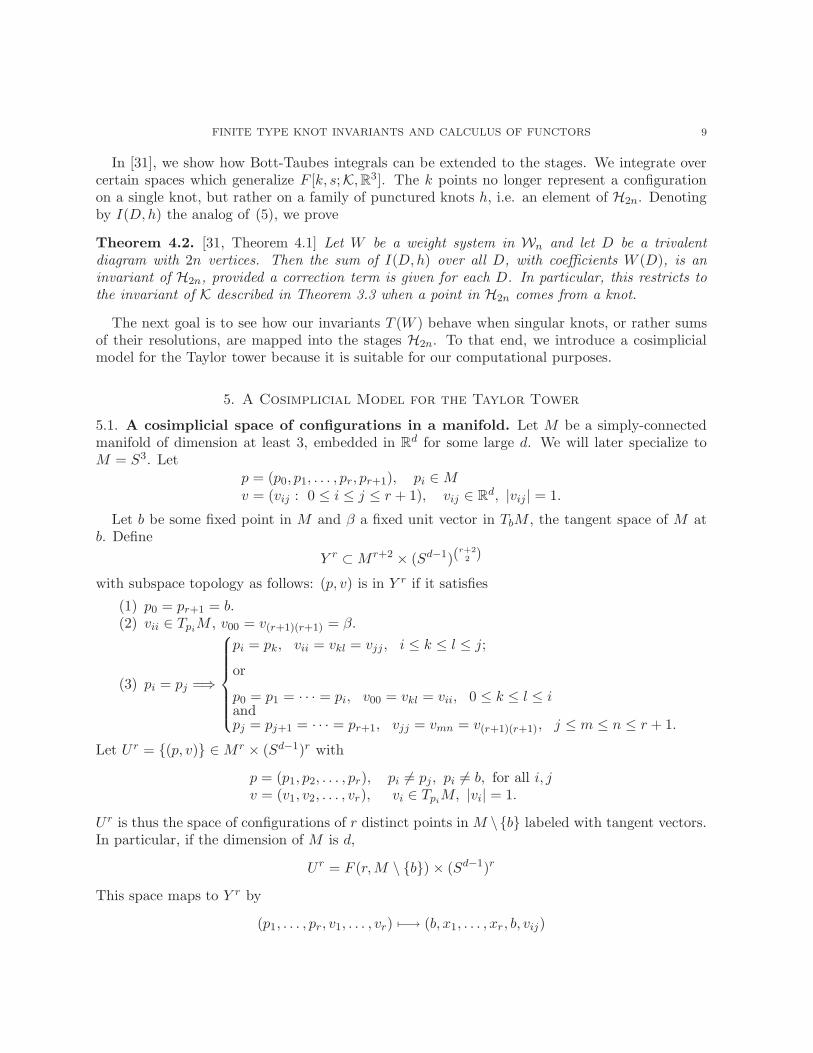
5.1. A cosimplicial space of configurations in a manifold. Let M be a simply-connectedmanifold of dimension at least 3, embedded in R

d for some large d. We will later specialize toM = S3. Let

p = (p0, p1, . . . , pr, pr+1), pi ∈Mv = (vij : 0 ≤ i ≤ j ≤ r + 1), vij ∈ R

d, |vij | = 1.

Let b be some fixed point in M and β a fixed unit vector in TbM , the tangent space of M atb. Define

Y r ⊂M r+2 × (Sd−1)(r+22 )

with subspace topology as follows: (p, v) is in Y r if it satisfies

(1) p0 = pr+1 = b.(2) vii ∈ Tpi

M , v00 = v(r+1)(r+1) = β.

(3) pi = pj =⇒

pi = pk, vii = vkl = vjj, i ≤ k ≤ l ≤ j;

or

p0 = p1 = · · · = pi, v00 = vkl = vii, 0 ≤ k ≤ l ≤ iandpj = pj+1 = · · · = pr+1, vjj = vmn = v(r+1)(r+1), j ≤ m ≤ n ≤ r + 1.

Let U r = (p, v) ∈M r × (Sd−1)r with

p = (p1, p2, . . . , pr), pi 6= pj, pi 6= b, for all i, jv = (v1, v2, . . . , vr), vi ∈ Tpi

M, |vi| = 1.

U r is thus the space of configurations of r distinct points in M \b labeled with tangent vectors.In particular, if the dimension of M is d,

U r = F (r,M \ b) × (Sd−1)r

This space maps to Y r by

(p1, . . . , pr, v1, . . . , vr) 7−→ (b, x1, . . . , xr, b, vij)

10 ISMAR VOLIC

where

vij =

vi, if 0 < i = j < m + 1;

β, if i = j = 0 or i = j = m + 1;pj−pi

|pj−pi|, if i < j.

It is easy to see that this map is one-to-one and a homeomorphism onto its image, so U r can beidentified with a subspace of Y r.

Definition 5.1. Let X0 = (b, b, β) and define Xr for all r > 0 to be the closure of U r in Y r.

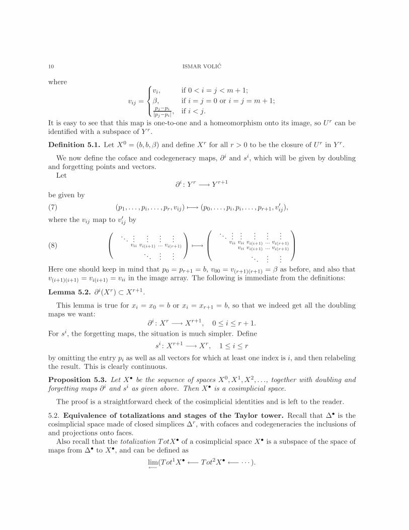
We now define the coface and codegeneracy maps, ∂i and si, which will be given by doublingand forgetting points and vectors.

Let∂i : Y r −→ Y r+1

be given by

(7) (p1, . . . , pi, . . . , pr, vij) 7−→ (p0, . . . , pi, pi, . . . , pr+1, v′ij),

where the vij map to v′ij by

(8)

. . ....

......

...vii vi(i+1) ... vi(r+1)

. . ....

...

7−→

. . ....

......

......

vii vii vi(i+1) ... vi(r+1)vii vi(i+1) ... vi(r+1)

. . ....

...

Here one should keep in mind that p0 = pr+1 = b, v00 = v(r+1)(r+1) = β as before, and also thatv(i+1)(i+1) = vi(i+1) = vii in the image array. The following is immediate from the definitions:

Lemma 5.2. ∂i(Xr) ⊂ Xr+1.

This lemma is true for xi = x0 = b or xi = xr+1 = b, so that we indeed get all the doublingmaps we want:

∂i : Xr −→ Xr+1, 0 ≤ i ≤ r + 1.

For si, the forgetting maps, the situation is much simpler. Define

si : Xr+1 −→ Xr, 1 ≤ i ≤ r

by omitting the entry pi as well as all vectors for which at least one index is i, and then relabelingthe result. This is clearly continuous.

Proposition 5.3. Let X• be the sequence of spaces X0,X1,X2, . . ., together with doubling andforgetting maps ∂i and si as given above. Then X• is a cosimplicial space.

The proof is a straightforward check of the cosimplicial identities and is left to the reader.

5.2. Equivalence of totalizations and stages of the Taylor tower. Recall that ∆• is thecosimplicial space made of closed simplices ∆r, with cofaces and codegeneracies the inclusions ofand projections onto faces.

Also recall that the totalization TotX• of a cosimplicial space X• is a subspace of the space ofmaps from ∆• to X•, and can be defined as

lim←−

(Tot1X• ←− Tot2X• ←− · · · ).


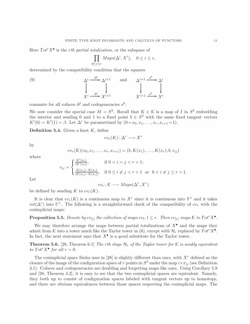
Here TotrX• is the rth partial totalization, or the subspace of∏

0≤i≤r

Maps(∆i,Xi), 0 ≤ i ≤ r,

determined by the compatibility condition that the squares

(9) ∆i∂j

//

∆i+1

Xi

∂j// Xi+1

and ∆i+1 sk//

∆i

Xi+1 sk

// Xi

commute for all cofaces ∂j and codegeneracies sk.

We now consider the special case M = S3. Recall that K ∈ K is a map of I in S3 embeddingthe interior and sending 0 and 1 to a fixed point b ∈ S3 with the same fixed tangent vectorsK ′(0) = K ′(1) = β. Let ∆r be parametrized by (0=x0, x1, . . . , xr, xr+1 =1).

Definition 5.4. Given a knot K, define

evr(K) : ∆r −→ Xr

byevr(K)(x0, x1, . . . , xr, xr+1) = (b,K(x1), . . . ,K(xr), b, vij)

where

vij =

K ′(xi)|K ′(xi)|

, if 0 < i = j < r + 1;

K(xj)−K(xi)|K(xj)−K(xi)|

, if 0 ≤ i 6= j < r + 1 or 0 < i 6= j ≤ r + 1.

Letevr : K −→Maps(∆r,Xr)

be defined by sending K to evr(K).

It is clear that evr(K) is a continuous map to Xr since it is continuous into Y r and it takesint(∆r) into U r. The following is a straightforward check of the compatibility of evr with thecosimplicial maps:

Proposition 5.5. Denote by ev[r] the collection of maps evl, l ≤ r. Then ev[r] maps K to TotrX•.

We may therefore arrange the maps between partial totalizations of X• and the maps theyadmit from K into a tower much like the Taylor tower in (6), except with Hr replaced by TotrX•.In fact, the next statement says that X• is a good substitute for the Taylor tower.

Theorem 5.6. [28, Theorem 6.1] The rth stage Hr of the Taylor tower for K is weakly equivalentto TotrX• for all r > 0.

The cosimplicial space Sinha uses in [28] is slightly different than ours, with Xr defined as theclosure of the image of the configuration space of r points in S3 under the map i×πij (see Definition3.1). Cofaces and codegeneracies are doubling and forgetting maps like ours. Using Corollary 5.9and [28, Theorem 4.2], it is easy to see that the two cosimplicial spaces are equivalent. Namely,they both up to consist of configuration spaces labeled with tangent vectors up to homotopy,and there are obvious equivalences between those spaces respecting the cosimplicial maps. The

12 ISMAR VOLIC

advantage of our definition is that it is made with knots and evaluation maps in mind (pointsmoving along a knot can only collide in one direction).

We next prove in Proposition 5.7 and Corollary 5.9 that ES (spaces of punctured knots) andXr are configurations labeled with tangent vectors. (The above theorem then in effect saysthat these configuration spaces are “put together the same way” in the homotopy limits andpartial totalizations. The main observations and tools in Sinha’s proof are that the restrictionmaps between punctured knots look like doubling maps up to homotopy and that a truncatedcosimplicial space can be redrawn as a subcubical diagram whose homotopy limit is equivalentto the original totalization. Sinha thus constructs equivalences going through an auxiliary towerwhose stages are homotopy limits of cubical diagrams of compactified configuration spaces withdoubling maps between them.)

Recall that ES is the space of embeddings of the complement of s = |S| closed subintervals in S3,where S is a nonempty subset of 1, . . . , r. In other words, each point in ES is an embedding ofs + 1 open subintervals (or half-open, in case of the first and last subinterval), which we index inorder from 1 to s + 1.

For each S and each open subinterval, choose points xi, 1 ≤ i ≤ s − 1, in the interiors. Thechoices should be compatible, namely if S ⊂ T , then xii∈S ⊂ xii∈T . Also let x0 and xs bethe left and right endpoints of I, respectively.

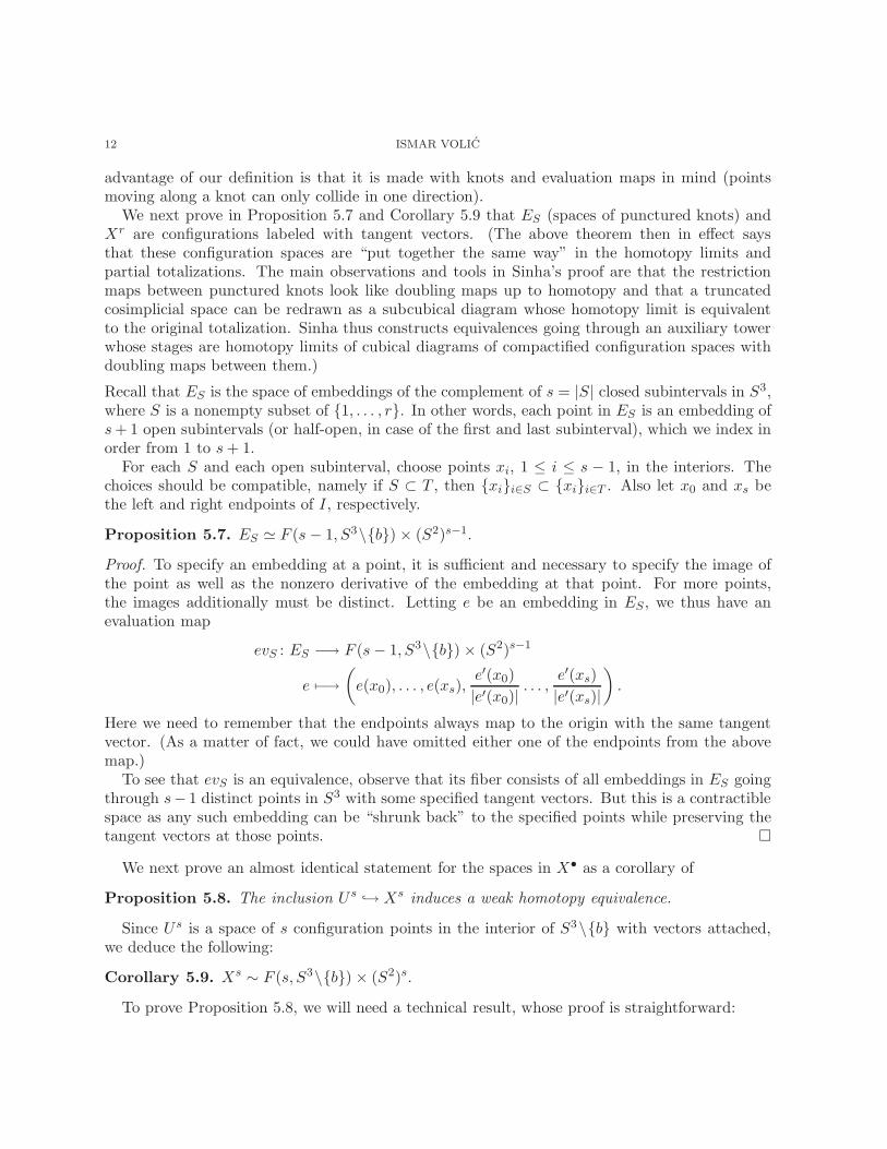
Proposition 5.7. ES ≃ F (s − 1, S3\b) × (S2)s−1.

Proof. To specify an embedding at a point, it is sufficient and necessary to specify the image ofthe point as well as the nonzero derivative of the embedding at that point. For more points,the images additionally must be distinct. Letting e be an embedding in ES , we thus have anevaluation map

evS : ES −→ F (s− 1, S3\b) × (S2)s−1

e 7−→

(e(x0), . . . , e(xs),

e′(x0)

|e′(x0)|. . . ,

e′(xs)

|e′(xs)|

).

Here we need to remember that the endpoints always map to the origin with the same tangentvector. (As a matter of fact, we could have omitted either one of the endpoints from the abovemap.)

To see that evS is an equivalence, observe that its fiber consists of all embeddings in ES goingthrough s− 1 distinct points in S3 with some specified tangent vectors. But this is a contractiblespace as any such embedding can be “shrunk back” to the specified points while preserving thetangent vectors at those points.

We next prove an almost identical statement for the spaces in X• as a corollary of

Proposition 5.8. The inclusion U s → Xs induces a weak homotopy equivalence.

Since U s is a space of s configuration points in the interior of S3\b with vectors attached,we deduce the following:

Corollary 5.9. Xs ∼ F (s, S3\b) × (S2)s.

To prove Proposition 5.8, we will need a technical result, whose proof is straightforward:


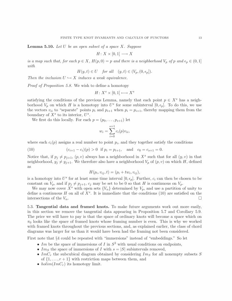
Lemma 5.10. Let U be an open subset of a space X. Suppose

H : X × [0, 1] −→ X

is a map such that, for each p ∈ X, H(p, 0) = p and there is a neighborhood Vp of p and ǫp ∈ (0, 1]with

H(y, t) ∈ U for all (y, t) ∈ (Vp, (0, ǫp]).

Then the inclusion U → X induces a weak equivalence.

Proof of Proposition 5.8. We wish to define a homotopy

H : Xs × [0, 1] 7−→ Xs

satisfying the conditions of the previous Lemma, namely that each point p ∈ Xs has a neigh-borhood Vp on which H is a homotopy into U s for some subinterval [0, ǫp]. To do this, we usethe vectors vii to “separate” points pi and pi+1 when pi = pi+1, thereby mapping them from theboundary of Xs to its interior, U s.

We first do this locally. For each p = (p0, . . . , ps+1) let

wi =s+1∑

i=0

ci(p)vii,

where each ci(p) assigns a real number to point pi, and they together satisfy the conditions

(10) (ci+1 − ci)(p) > 0 if pi = pi+1, and c0 = cs+1 = 0.

Notice that, if pj 6= pj+1, (p, v) always has a neighborhood in Xs such that for all (y, v) in thatneighborhood, yj 6= yj+1. We therefore also have a neighborhood Vp of (p, v) on which H, definedas

H(pi, vij , t) = (pi + twi, vij),

is a homotopy into U s for at least some time interval [0, ǫp]. Further, ci can then be chosen to beconstant on Vp, and if pj 6= pj+1, cj may be set to be 0 so that H is continuous on Vp.

We may now cover Xs with open sets Vα determined by Vp, and use a partition of unity todefine a continuous H on all of Xs. It is immediate that the conditions (10) are satisfied on theintersections of the Vα.

5.3. Tangential data and framed knots. To make future arguments work out more easily,in this section we remove the tangential data appearing in Proposition 5.7 and Corollary 5.9.The price we will have to pay is that the space of ordinary knots will become a space which onπ0 looks like the space of framed knots whose framing number is even. This is why we workedwith framed knots throughout the previous sections, and, as explained earlier, the class of chorddiagrams was larger for us than it would have been had the framing not been considered.

First note that §4 could be repeated with “immersions” instead of “embeddings.” So let

• Im be the space of immersions of I in S3 with usual conditions on endpoints,• ImS the space of immersions of I with s = |S| subintervals removed,• ImCr the subcubical diagram obtained by considering ImS for all nonempty subsets S

of 1, . . . , r + 1 with restriction maps between them, and• holim(ImCr) its homotopy limit.

14 ISMAR VOLIC

Recall that Im is homotopy equivalent to ΩS2 since immersions are determined by their deriva-tives. Similarly, in analogy with Proposition 5.7, we have

(11) ImS ≃ (S2)s−1.

The configuration space is no longer present in the equivalence because of the lack of the injectivitycondition for immersions.

Before we prove two useful statements, we need

Proposition 5.11 ([14], Proposition 1.6.). Suppose X∅ completes a subcubical diagram Cr ofspaces XS indexed by nonempty subsets of 1, . . . , r into a cubical diagram. If, for every S,

XS −→ holim(XS∪j → XS∪i,j ← XS∪i)

is a weak equivalence, then X∅ → holim(Cr) is a weak equivalence as well.

Proposition 5.12. Im −→ holim(ImCr) is a weak equivalence.

Proof. Unlike for spaces of punctured embeddings, ImS is the limit of

(12) ImS∪j // ImS∪i,j ImS∪ioo

Further, the map ImS → ImS∪i is a fibration for all i. It follows that ImS is weakly equivalentto the homotopy limit of diagram (12). This holds for any square in ImCr. In addition, we cancomplete the subcube ImCr by adding Im as the initial space. For the extra square diagramsproduced this way, we again have that Im is equivalent to their homotopy limits. Proposition 5.11then finishes the proof.

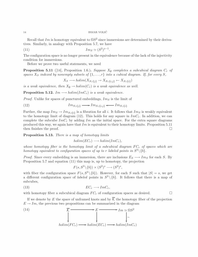
Proposition 5.13. There is a map of homotopy limits

holim(ECr) −→ holim(ImCr),

whose homotopy fiber is the homotopy limit of a subcubical diagram FCr of spaces which arehomotopy equivalent to configuration spaces of up to r labeled points in S3\b.

Proof. Since every embedding is an immersion, there are inclusions ES −→ ImS for each S. ByProposition 5.7 and equation (11) this map is, up to homotopy, the projection

F (s, S3\b) × (S2)s −→ (S2)s,

with fiber the configuration space F (s, S3\b). However, for each S such that |S| = s, we geta different configuration space of labeled points in S3 \b. It follows that there is a map ofsubcubes,

(13) ECr −→ ImCr,

with homotopy fiber a subcubical diagram FCr of configuration spaces as desired.

If we denote by E the space of unframed knots and by K the homotopy fiber of the projectionE → Im, the previous two propositions can be summarized in the diagram

(14) K //

E //

Im ≃ ΩS2

∼

holim(FCr) // holim(ECr) // holim(ImCr)


where the left spaces are the homotopy fibers of the two right horizontal maps.The middle column in the diagram represents the spaces and maps we would have originally

considered, but since we wish to remove the tangent spheres, we now shift our attention to theleft column. Since the map E → Im is null-homotopic [26, Proposition 5.1], we have

K ≃ E × ΩIm.

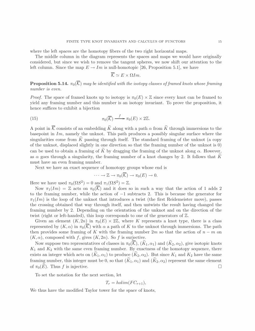
Proposition 5.14. π0(K) may be identified with the isotopy classes of framed knots whose framingnumber is even.

Proof. The space of framed knots up to isotopy is π0(E) × Z since every knot can be framed toyield any framing number and this number is an isotopy invariant. To prove the proposition, ithence suffices to exhibit a bijection

(15) π0(K)f // π0(E)× 2Z.

A point in K consists of an embedding K along with a path α from K through immersions to thebasepoint in Im, namely the unknot. This path produces a possibly singular surface where the

singularities come from K passing through itself. The standard framing of the unknot (a copyof the unknot, displaced slightly in one direction so that the framing number of the unknot is 0)

can be used to obtain a framing of K by dragging the framing of the unknot along α. However,

as α goes through a singularity, the framing number of a knot changes by 2. It follows that Kmust have an even framing number.

Next we have an exact sequence of homotopy groups whose end is

· · · → Z→ π0(K)→ π0(E)→ 0.

Here we have used π0(ΩS2) = 0 and π1(ΩS2) = Z.Now π1(Im) = Z acts on π0(K) and it does so in such a way that the action of 1 adds 2

to the framing number, while the action of −1 subtracts 2. This is because the generator forπ1(Im) is the loop of the unknot that introduces a twist (the first Reidemeister move), passesthe crossing obtained that way through itself, and then untwists the result having changed theframing number by 2. Depending on the orientation of the unknot and on the direction of thetwist (right or left-handed), this loop corresponds to one of the generators of Z.

Given an element (K, 2n) in π0(E) × 2Z, where K represents a knot type, there is a classrepresented by (K,α) in π0(K) with α a path of K to the unknot through immersions. The paththen provides some framing of K with the framing number 2m so that the action of n −m on(K,α), composed with f , gives (K, 2n). So f is surjective.

Now suppose two representatives of classes in π0(K), (K1, α1) and (K2, α2), give isotopic knotsK1 and K2 with the same even framing number. By exactness of the homotopy sequence, there

exists an integer which acts on (K1, α1) to produce (K2, α2). But since K1 and K2 have the same

framing number, this integer must be 0, so that (K1, α1) and (K2, α2) represent the same element

of π0(E). Thus f is injective.

To set the notation for the next section, let

Tr = holim(FCr+1),

We thus have the modified Taylor tower for the space of knots,

16 ISMAR VOLIC

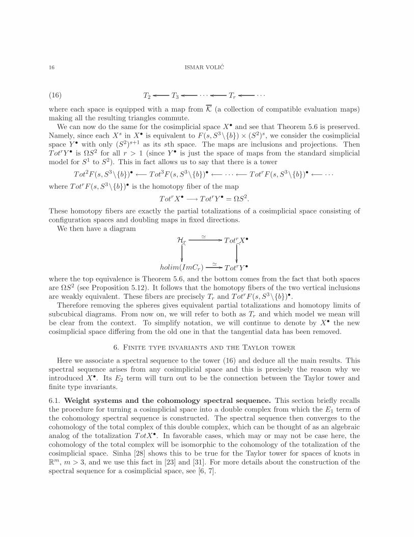
(16) T2 T3oo · · ·oo Tr

oo · · ·oo

where each space is equipped with a map from K (a collection of compatible evaluation maps)making all the resulting triangles commute.

We can now do the same for the cosimplicial space X• and see that Theorem 5.6 is preserved.Namely, since each Xs in X• is equivalent to F (s, S3\b) × (S2)s, we consider the cosimplicialspace Y • with only (S2)s+1 as its sth space. The maps are inclusions and projections. ThenTotrY • is ΩS2 for all r > 1 (since Y • is just the space of maps from the standard simplicialmodel for S1 to S2). This in fact allows us to say that there is a tower

Tot2F (s, S3\b)• ←− Tot3F (s, S3\b)• ←− · · · ←− TotrF (s, S3\b)• ←− · · ·

where TotrF (s, S3\b)• is the homotopy fiber of the map

TotrX• −→ TotrY • = ΩS2.

These homotopy fibers are exactly the partial totalizations of a cosimplicial space consisting ofconfiguration spaces and doubling maps in fixed directions.

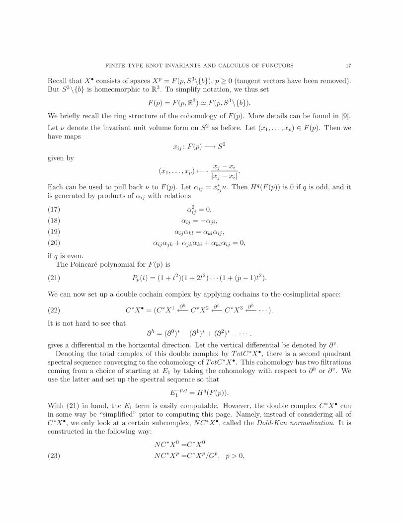
We then have a diagram

Hr _

≃ // TotrX• _

holim(ImCr)

≃ // TotrY •

where the top equivalence is Theorem 5.6, and the bottom comes from the fact that both spacesare ΩS2 (see Proposition 5.12). It follows that the homotopy fibers of the two vertical inclusionsare weakly equivalent. These fibers are precisely Tr and TotrF (s, S3\b)•.

Therefore removing the spheres gives equivalent partial totalizations and homotopy limits ofsubcubical diagrams. From now on, we will refer to both as Tr and which model we mean willbe clear from the context. To simplify notation, we will continue to denote by X• the newcosimplicial space differing from the old one in that the tangential data has been removed.

6. Finite type invariants and the Taylor tower

Here we associate a spectral sequence to the tower (16) and deduce all the main results. Thisspectral sequence arises from any cosimplicial space and this is precisely the reason why weintroduced X•. Its E2 term will turn out to be the connection between the Taylor tower andfinite type invariants.

6.1. Weight systems and the cohomology spectral sequence. This section briefly recallsthe procedure for turning a cosimplicial space into a double complex from which the E1 term ofthe cohomology spectral sequence is constructed. The spectral sequence then converges to thecohomology of the total complex of this double complex, which can be thought of as an algebraicanalog of the totalization TotX•. In favorable cases, which may or may not be case here, thecohomology of the total complex will be isomorphic to the cohomology of the totalization of thecosimplicial space. Sinha [28] shows this to be true for the Taylor tower for spaces of knots inR

m, m > 3, and we use this fact in [23] and [31]. For more details about the construction of thespectral sequence for a cosimplicial space, see [6, 7].


Recall that X• consists of spaces Xp = F (p, S3\b), p ≥ 0 (tangent vectors have been removed).But S3\b is homeomorphic to R

3. To simplify notation, we thus set

F (p) = F (p, R3) ≃ F (p, S3\b).

We briefly recall the ring structure of the cohomology of F (p). More details can be found in [9].

Let ν denote the invariant unit volume form on S2 as before. Let (x1, . . . , xp) ∈ F (p). Then wehave maps

xij : F (p) −→ S2

given by

(x1, . . . , xp) 7−→xj − xi

|xj − xi|.

Each can be used to pull back ν to F (p). Let αij = x∗ijν. Then Hq(F (p)) is 0 if q is odd, and itis generated by products of αij with relations

α2ij = 0,(17)

αij = −αji,(18)

αijαkl = αklαij ,(19)

αijαjk + αjkαki + αkiαij = 0,(20)

if q is even.The Poincare polynomial for F (p) is

(21) Pp(t) = (1 + t2)(1 + 2t2) · · · (1 + (p − 1)t2).

We can now set up a double cochain complex by applying cochains to the cosimplicial space:

(22) C∗X• = (C∗X1 ∂h

←− C∗X2 ∂h

←− C∗X3 ∂h

←− · · · ).

It is not hard to see that

∂h = (∂0)∗ − (∂1)∗ + (∂2)∗ − · · · .

gives a differential in the horizontal direction. Let the vertical differential be denoted by ∂v .Denoting the total complex of this double complex by TotC∗X•, there is a second quadrant

spectral sequence converging to the cohomology of TotC∗X•. This cohomology has two filtrationscoming from a choice of starting at E1 by taking the cohomology with respect to ∂h or ∂v . Weuse the latter and set up the spectral sequence so that

E−p,q1 = Hq(F (p)).

With (21) in hand, the E1 term is easily computable. However, the double complex C∗X• canin some way be “simplified” prior to computing this page. Namely, instead of considering all ofC∗X•, we only look at a certain subcomplex, NC∗X•, called the Dold-Kan normalization. It isconstructed in the following way:

NC∗X0 =C∗X0

NC∗Xp =C∗Xp/Gp, p > 0,(23)

18 ISMAR VOLIC

where Gp is the subgroup generated by

(24)

p−1∑

i=0

Im(C∗Xp−1 (si)∗−→ C∗Xp)).

This normalization can be applied to any double complex obtained from a simplicial or acosimplicial space. The important feature is that TotNC∗X• has the same cohomology asTotC∗X•. The normalization in general can be thought of as throwing away the degeneratepart of a (co)simplicial complex.

Let Gp,n be the subgroup of H2n(F (p)) generated by the images of

(si)∗ : H2n(F (p − 1)) −→ H2n(F (p)).

Then the normalized E1 has entries

E−p,2n1 = H2n

norm(F (p)) = H2n(F (p))/Gp,n.

Choose a basis for H2n(F (p)) using relations (17)–(20) by letting

α = αi1j1αi2j2 · · ·αikjk, im, jm ∈ 1, . . . , p,

be a generator of H2n(F (p)). Then α is a basis element if

ia = ib =⇒ ja 6= jb,(25)

ia < ja,(26)

j1 < j2 < · · · < jk,(27)

The first observation is

Lemma 6.1. If 2n < p, then H2nnorm = 0.

Proof. Since 2n < p, it follows that some point xr in F (p) was not used in any xij. Now apply thecodegeneracy sr : F (p) −→ F (p − 1) by forgetting xr and relabeling the result. Then xi ∈ F (p)remains xi ∈ F (p − 1) if i < r, and becomes xi−1 ∈ F (p− 1) if i > r.

Now let α′ be a class in H2n(F (p − 1)) constructed from the maps x′ij such that

(28) x′ij =

xi(j−1), if i < r < j;

x(i−1)(j−1), if r < i < j;

xij , if i < j < r.

But by construction, composing the product of the x′ij with sr yields precisely α. Thus α is inthe image of

(sr)∗ : H2n(F (p − 1)) −→ H2n(F (p)).

The discussion in the preceding proof can be extended to other cases. Regardless of the relationbetween 2n and p, we can still conclude that if a class α is obtained without using all the pointsin the configuration, some codegeneracy induces a map on cohomology with α in its image.

On the other hand, if α is obtained by using all the points, then for every codegeneracy si, amap on F (p) involving xi becomes undefined on F (p− 1). Thus α is not in the image of (si)∗ forany i, nor is it in the subspace generated by them as the image of each codegeneracy is generatedby a part of the basis. Hence α survives to H2n

norm(F (p)). For the same reason, all such α remain


independent after normalization. It follows therefore that a basis element α in H2nnorm(F (p)) can

be described by simply adding one more requirement to conditions (25)–(27):

(29) For every xi ∈ F (p), i must occur as a subscript in α.

It is convenient at this stage to switch the point of view from cohomology to homology forestablishing a clear connection between the Taylor tower (and its cosimplicial model) and finitetype knot invariants.

Given a basis element α = αi1j1αi2j2 · · ·αinjn ∈ H2nnorm(F (p)), let a = ai1j1i2j2···injn denote its

dual in Hnorm2n (F (p)). (By Hnorm

2n (F (p)) we mean the homology obtained by considering chainson X•, using the alternating sums of (∂i)∗ to obtain a chain complex in one direction, and thennormalizing it via a dual version of (23).) An element a ∈ Hnorm

2n (F (p)) can be thought of as achord diagram oriented by p labeled points which are connected by oriented chords as prescribedby pairs of indices in a. Thus i1 is connected to j1 and the arrow on the chord points from i1;i2 is connected to j2 with the arrow pointing from i2, etc. We also impose the following signconvention: If two basis elements a and a′ differ by τ transpositions of their subscripts, thena = (−1)τa′. Thus we choose any element a and a sign for it, and then apply the sign convention.It is easy to see that this is a well-defined assignment.

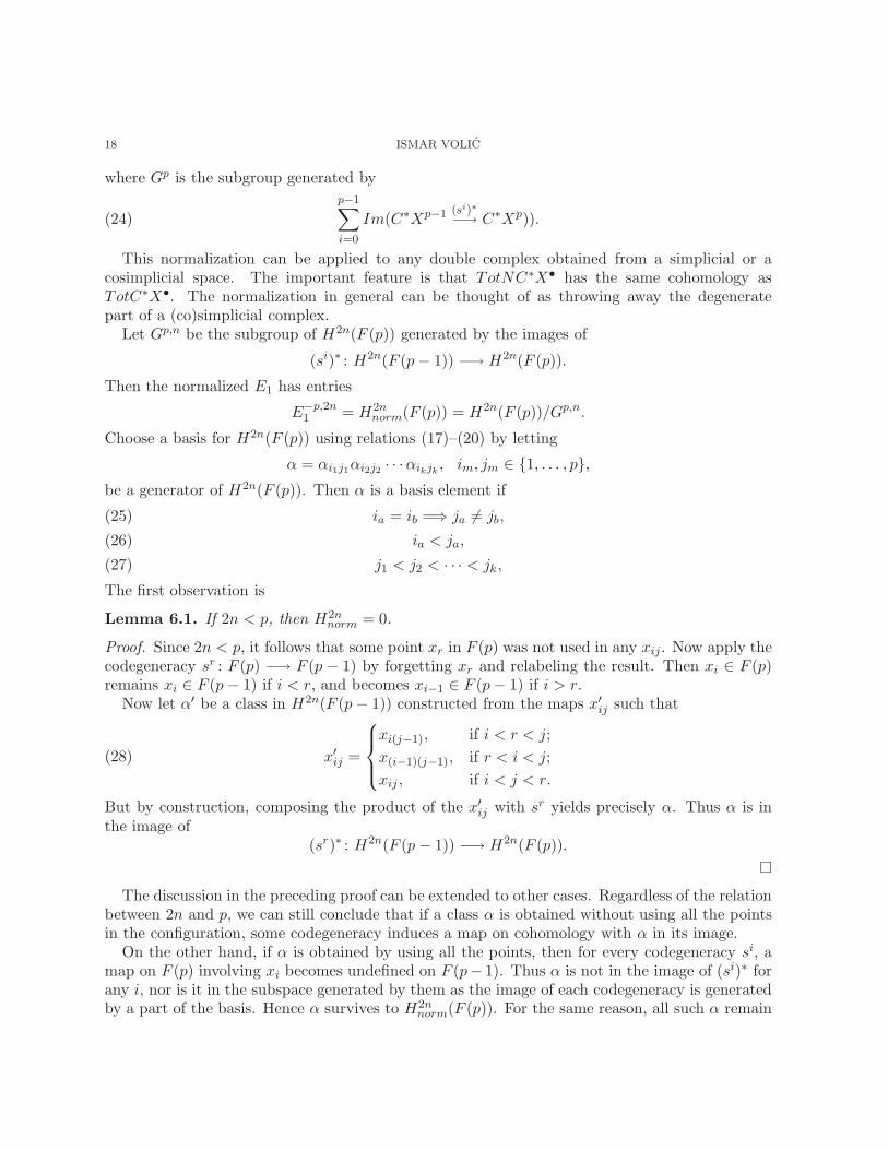
Conversely, take a free module generated by chord diagrams with p labeled vertices and noriented chords, and consider its quotient obtained by imposing the relations

(1) If a chord in a diagram D connects the same vertex, then D = 0;(2) If two chords in D connect the same vertices, then D = 0;(3) If two diagrams D1 and D2 differ by a change of orientation of a chord or by a transposition

of two vertex labels, then D = −D′;(4) Let i < j < k. If

D1 contains two chords connecting vertices i, j and j, k;

D2 contains two chords connecting vertices i, j and i, k;

D3 contains two chords connecting vertices i, k and j, k;

then D3 = −D1 −D2.

It follows by construction that Hnorm2n (F (p)) is isomorphic to this quotient. In the most relevant

case for us, p = 2n, every vertex of a chord diagram must then have exactly one chord connectingit to some other vertex. But this is precisely the description of CDn. We thus have the followingsimple but important statement:

Proposition 6.2. E1−2n,2n = Hnorm

2n (F (2n)) is generated by CDn.

The next proposition states that the first differential introduces precisely the 4T relation of§2. We prove the dual version because the combinatorics of the proof will be more transparent.Remember that the space of weight systems Wn was defined as functions on R[CDn] vanishingon the 4T relation.

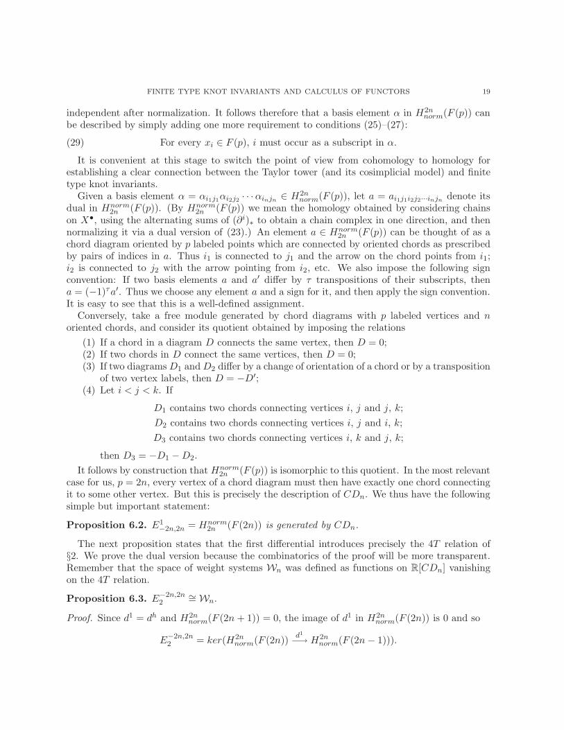
Proposition 6.3. E−2n,2n2

∼=Wn.

Proof. Since d1 = dh and H2nnorm(F (2n + 1)) = 0, the image of d1 in H2n

norm(F (2n)) is 0 and so

E−2n,2n2 = ker(H2n

norm(F (2n))d1

−→ H2nnorm(F (2n − 1))).

20 ISMAR VOLIC

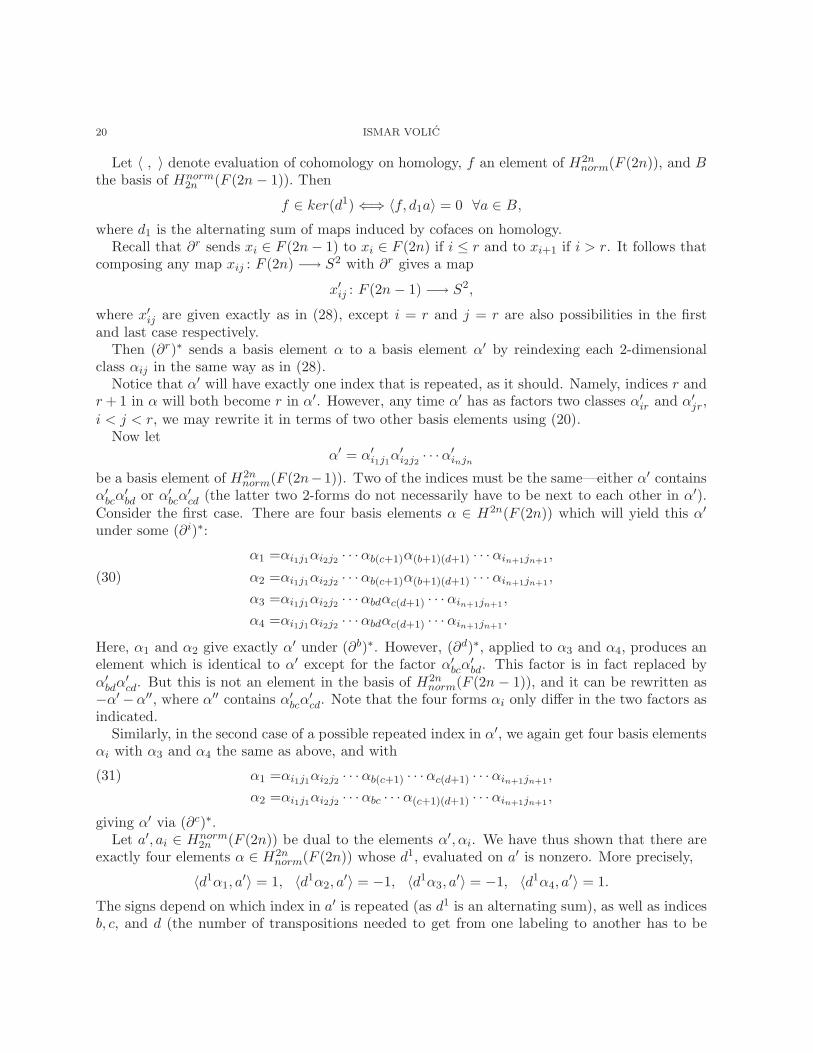
Let 〈 , 〉 denote evaluation of cohomology on homology, f an element of H2nnorm(F (2n)), and B

the basis of Hnorm2n (F (2n − 1)). Then

f ∈ ker(d1)⇐⇒ 〈f, d1a〉 = 0 ∀a ∈ B,

where d1 is the alternating sum of maps induced by cofaces on homology.Recall that ∂r sends xi ∈ F (2n− 1) to xi ∈ F (2n) if i ≤ r and to xi+1 if i > r. It follows that

composing any map xij : F (2n) −→ S2 with ∂r gives a map

x′ij : F (2n − 1) −→ S2,

where x′ij are given exactly as in (28), except i = r and j = r are also possibilities in the firstand last case respectively.

Then (∂r)∗ sends a basis element α to a basis element α′ by reindexing each 2-dimensionalclass αij in the same way as in (28).

Notice that α′ will have exactly one index that is repeated, as it should. Namely, indices r andr + 1 in α will both become r in α′. However, any time α′ has as factors two classes α′ir and α′jr,

i < j < r, we may rewrite it in terms of two other basis elements using (20).Now let

α′ = α′i1j1α′i2j2

· · ·α′injn

be a basis element of H2nnorm(F (2n−1)). Two of the indices must be the same—either α′ contains

α′bcα′bd or α′bcα

′cd (the latter two 2-forms do not necessarily have to be next to each other in α′).

Consider the first case. There are four basis elements α ∈ H2n(F (2n)) which will yield this α′

under some (∂i)∗:

α1 =αi1j1αi2j2 · · ·αb(c+1)α(b+1)(d+1) · · ·αin+1jn+1,

α2 =αi1j1αi2j2 · · ·αb(c+1)α(b+1)(d+1) · · ·αin+1jn+1,(30)

α3 =αi1j1αi2j2 · · ·αbdαc(d+1) · · ·αin+1jn+1,

α4 =αi1j1αi2j2 · · ·αbdαc(d+1) · · ·αin+1jn+1.

Here, α1 and α2 give exactly α′ under (∂b)∗. However, (∂d)∗, applied to α3 and α4, produces anelement which is identical to α′ except for the factor α′bcα

′bd. This factor is in fact replaced by

α′bdα′cd. But this is not an element in the basis of H2n

norm(F (2n − 1)), and it can be rewritten as−α′−α′′, where α′′ contains α′bcα

′cd. Note that the four forms αi only differ in the two factors as

indicated.Similarly, in the second case of a possible repeated index in α′, we again get four basis elements

αi with α3 and α4 the same as above, and with

α1 =αi1j1αi2j2 · · ·αb(c+1) · · ·αc(d+1) · · ·αin+1jn+1,(31)

α2 =αi1j1αi2j2 · · ·αbc · · ·α(c+1)(d+1) · · ·αin+1jn+1,

giving α′ via (∂c)∗.Let a′, ai ∈ Hnorm

2n (F (2n)) be dual to the elements α′, αi. We have thus shown that there areexactly four elements α ∈ H2n

norm(F (2n)) whose d1, evaluated on a′ is nonzero. More precisely,

〈d1α1, a′〉 = 1, 〈d1α2, a

′〉 = −1, 〈d1α3, a′〉 = −1, 〈d1α4, a

′〉 = 1.

The signs depend on which index in a′ is repeated (as d1 is an alternating sum), as well as indicesb, c, and d (the number of transpositions needed to get from one labeling to another has to be


taken into account). So

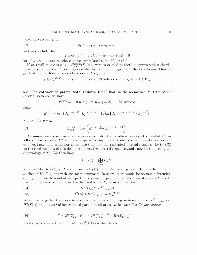
(32) d1a′ = a1 − a2 − a3 + a4,

and we conclude thatf ∈ ker(d1)⇐⇒ 〈f, a1 − a2 − a3 + a4〉 = 0

for all a1, a2, a3, and a4 whose indices are related as in (30) or (31).If we recall that classes a ∈ Hnorm

2n (F (2n)) were associated to chord diagrams with n chords,then the conditions on ai precisely describe the four chord diagrams in the 4T relation. Thus weget that, if f is thought of as a function on CDn, then

f ∈ E−2n,2n2 ⇐⇒ 〈f, 4T 〉 = 0 for all 4T relations in CDn ⇐⇒ f ∈ Wn.

6.2. The cotower of partial totalizations. Recall that, in the normalized E2 term of thespectral sequence, we have

E−p,q2 = 0 if p < q or p = q = 2k + 1 for some k.

Since

E−p,qi+1 = ker

(E−p,q

i

di

−→ E−p+i,q−i+1i

)/im

(E−p−i,q+i−1

i

di

−→ E−p,qi

),

we have, for p = q,

(33) E−p,pi+1 = ker

(E−p,p

i

di

−→ E−p+i,p−i+1i

).

An immediate consequence is that we can construct an algebraic analog of Tr, called T ∗r , asfollows: We truncate X• at the rth space for any r, and then construct the double cochaincomplex (now finite in the horizontal direction) and the associated spectral sequence. Letting T ∗rbe the total complex of this double complex, the spectral sequence would now be computing thecohomology of T ∗r . We then have

H0(T ∗r ) =

r⊕

j=0

E−j,j∞ .

Now consider H0(T ∗r+1). A consequence of (33) is that its grading would be exactly the same

as that of H0(T ∗r ), but with one more summand. In short, there would be no new differentialscoming into the diagonal of the spectral sequence in passing from the truncation of X• at r tor + 1. Since every odd entry on the diagonal at the E2 term is 0, we conclude

H0(T ∗2n) ∼= H0(T ∗2n+1)(34)

H0(T ∗2n)/H0(T ∗2n−1)∼= E−2n,2n

∞ .(35)

We can put together the above isomorphisms (the second giving an injection from H0(T ∗2n−1) to

H0(T ∗2n)) into a tower of invariants of partial totalizations which we call a Taylor cotower :

(36) · · ·∼= // H0(T ∗2n−1)

// H0(T ∗2n)∼= // H0(T ∗2n+1)

// · · ·

Each space comes with a map ev∗[i] to H0(K) described below.

22 ISMAR VOLIC

Remark. Going from partial totalizations Tr = TotrX• to total complexes T ∗r = TotrC∗X• is alsopossible directly from the subcubical diagrams of configuration spaces. We have bypassed this byworking with X• instead, but we could have also considered cochains on all spaces of puncturedembeddings in the subcubical diagram (all arrows would now get reversed) and then formed thehomotopy colimit hocolim(C∗FCr) (dual to the homotopy limit, but now in an algebraic sense).A double complex T ∗r could then be formed by collecting all cochains on embeddings with thesame number of punctures.

6.3. The evaluation map to finite type invariants. Let ev∗[i] be the map induced by ev[i] on

cochains on configurations and cohomology:

ev∗[i] : H0(TotiC∗X•) = H0(T ∗i ) −→ H0(K).

To simplify notation, we set ev∗ = ev∗[i] for all i. Which value of i is used will be clear from the

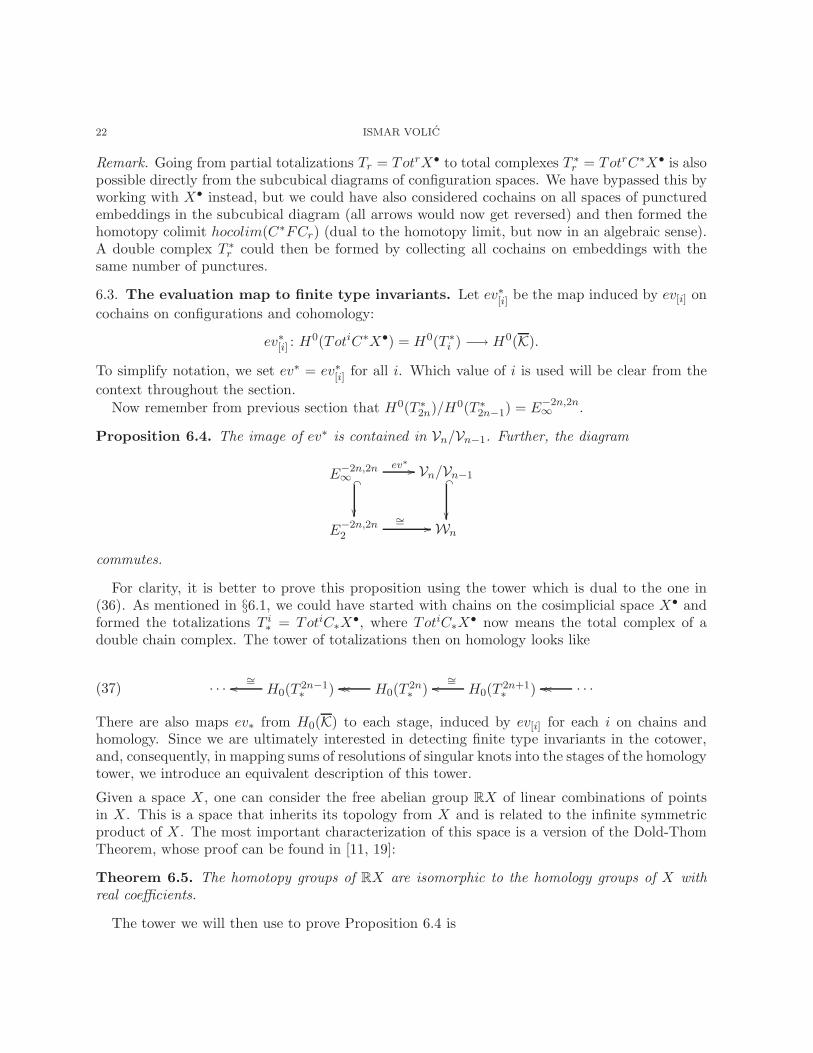
context throughout the section.Now remember from previous section that H0(T ∗2n)/H0(T ∗2n−1) = E−2n,2n

∞ .

Proposition 6.4. The image of ev∗ is contained in Vn/Vn−1. Further, the diagram

E−2n,2n∞

ev∗ // _

Vn/Vn−1 _

E−2n,2n

2

∼= // Wn

commutes.

For clarity, it is better to prove this proposition using the tower which is dual to the one in(36). As mentioned in §6.1, we could have started with chains on the cosimplicial space X• andformed the totalizations T i

∗ = TotiC∗X•, where TotiC∗X

• now means the total complex of adouble chain complex. The tower of totalizations then on homology looks like

(37) · · · H0(T2n−1∗ )

∼=oo H0(T2n∗ )oooo H0(T

2n+1∗ )

∼=oo · · ·oooo

There are also maps ev∗ from H0(K) to each stage, induced by ev[i] for each i on chains andhomology. Since we are ultimately interested in detecting finite type invariants in the cotower,and, consequently, in mapping sums of resolutions of singular knots into the stages of the homologytower, we introduce an equivalent description of this tower.

Given a space X, one can consider the free abelian group RX of linear combinations of pointsin X. This is a space that inherits its topology from X and is related to the infinite symmetricproduct of X. The most important characterization of this space is a version of the Dold-ThomTheorem, whose proof can be found in [11, 19]:

Theorem 6.5. The homotopy groups of RX are isomorphic to the homology groups of X withreal coefficients.

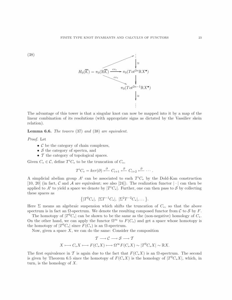
The tower we will then use to prove Proposition 6.4 is


(38) ...

∼=

H0(K) = π0(RK)

ev∗ //

ev∗

))SSSSSSSSSSSSSS

55llllllllllllllllll

π0(Tot2nRX•)

π0(Tot2n−1

RX•)

∼=...

The advantage of this tower is that a singular knot can now be mapped into it by a map of thelinear combination of its resolutions (with appropriate signs as dictated by the Vassiliev skeinrelation).

Lemma 6.6. The towers (37) and (38) are equivalent.

Proof. Let

• C be the category of chain complexes,• S the category of spectra, and• T the category of topological spaces.

Given C∗ ∈ C, define T iC∗ to be the truncation of C∗,

T iC∗ = ker(∂)∂←− Ci+1

∂←− Ci+2

∂←− · · · .

A simplicial abelian group Ai can be associated to each T iC∗ by the Dold-Kan construction[10, 20] (in fact, C and A are equivalent; see also [24]). The realization functor | · | can then beapplied to Ai to yield a space we denote by |T iC∗|. Further, one can then pass to S by collectingthese spaces as

|T 0C∗|, |ΣT−1C∗|, |Σ2T−2C∗|, . . .

.

Here Σ means an algebraic suspension which shifts the truncation of C∗, so that the abovespectrum is in fact an Ω-spectrum. We denote the resulting composed functor from C to S by F .

The homotopy of |T 0C∗| can be shown to be the same as the (non-negative) homology of C∗.On the other hand, we can apply the functor Ω∞ to F (C∗) and get a space whose homotopy isthe homotopy of |T 0C∗| since F (C∗) is an Ω-spectrum.

Now, given a space X, we can do the same: Consider the composition

T −→ C −→ S −→ T

X 7−→ C∗X 7−→ F (C∗X) 7−→ Ω∞F (C∗X) ∼ |T 0C∗X| ∼ RX.

The first equivalence in T is again due to the fact that F (C∗X) is an Ω-spectrum. The secondis given by Theorem 6.5 since the homotopy of F (C∗X) is the homology of |T 0C∗X|, which, inturn, is the homology of X.

24 ISMAR VOLIC

But we can go even further, and start with a cosimplicial space X• (or any diagram of spacesviewed as a functor from an indexing category to T ). A generalized version of the above producesa cosimplicial spectrum F (C∗X

•) and we get a composition of functors

X• 7−→ C∗X• 7−→ F (C∗X

•) 7−→ Ω∞F (C∗X•) ∼ RX•.

In particular, from the weak equivalence in above, we can deduce

(39) Totr(Ω∞F (C∗X•)) ∼ Totr(RX•),

for all partial totalizations Totr.

Remarks. Totalization only preserves equivalences, however, if X• is a fibrant cosimplicial space.Every cosimplicial space can be replaced by a fibrant one via a degreewise equivalence of cosimpli-cial spaces and in fact our cosimplicial space had to be replaced by a fibrant one for Theorem 5.6to be true anyway.

For a more general diagram of spaces, the role of the totalization is played by the homotopylimit of the diagram.

Next we have

(40) Ω∞F (TotrC∗X•) ∼ Ω∞Totr(F (C∗X

•)) ∼ Totr(Ω∞F (C∗X•)).

The second equivalence is true because the functor Totr is defined as a compatible collectionof spaces Maps(∆i,Xi), i ≤ r, and Ω Maps(∆i,Xi) ∼ Maps(∆i,ΩXi). Essentially the samereasoning applies in the case of the first equivalence, except the argument is not as straightfor-ward since TotrC∗X

• is an algebraic construction involving total complexes rather than mappingspaces.

But we also know that there is an equivalence

(41) Ω∞F (TotrC∗X•) ∼ TotrRX.

In particular, putting (39), (40), and (41) together on π0, we have

π0(TotrRX•) = H0(TotrC∗X•).

Since the tower (37) had H0(TotrC∗X•) = H0(T

r∗ ) as its stages, we can now replace them by

π0(TotrRX•).

Proof of Proposition 6.4. The idea will be that an n-singular knot maps to Tot2n−1RX• via the

evaluation map, but the map is homotopic to 0. However, the homotopy cannot be extendedto Tot2n

RX• and the obstruction to doing so is precisely the chord diagram associated to thesingular knot.

So let K be an n-singular knot, and let a1, . . . , an, b1, . . . , bn be the points in the interior ofI = [0, 1] making up the singularities, i.e. K(ai) = K(bi). Let t = (t1, . . . , tj) be a point in ∆j

and note that for all j we are considering, j < 2n. The fact that there are always fewer ti thanai and bi is crucial in what follows.

Now pick closed intervals Ik, Jk around the points ak, bk so that the 2n resolutions of K differonly in the K(Ik). Let the resolutions be indexed by the subsets S of 1, 2, . . . , n in the sensethat if k ∈ S, then K(Ik) was changed into an overstrand (in the Vassiliev skein relation).

It is clear how to extend ev to linear combinations of knots and get a map

ev : RK −→ (∆j → RXj).


In particular, we can map sums of resolutions KS (taken with appropriate signs) of an n-singularknot.

Let

e+k = KS(Ik), if k ∈ S,

e−k = KS(Ik), if k /∈ S,

and define a homotopy (parametrized by u)

euk = (1− u)e+

k + ue−k .

Note that this homotopy is only defined on Ik and has the effect of changing an overcrossing toan undercrossing. The problem is that, for some time u, this homotopy reintroduces the originalsingularity on the resolved knot. This means that ev will yield a degenerate configuration if anytwo of the ti equal ak and bk.

To avoid this, it suffices to modify the homotopy so that no movement takes place when thereis some ti ∈ ∆j which equals bk. To do this, define a map

φk(t) : ∆j −→ [0, 1]

by

φk(t) =

2minl(|tl−bk|)

|Jk|, if at least one of the ti is in Jk;

1, otherwise.

Then φk(t) is a continuous map which is 0 if, for any i, ti = bk and 1 if, for all i, ti /∈ Jk.Now let

eu,tS =

euφk(t)k , in Ik if k ∈ S;

KS , outside Ik for all k.

Thus eu,tS changes overcrossing KS(Ik) to undercrossing KS(Jk) if no ti is in Jk. If some ti

enters Jk, the homotopy happens only part of the way. If any ti comes to the center of Jk andthus equals bk, the homotopy is just constant.

This setup then prevents the collision of configuration points in Xj so that it makes sense touse ev to define a homotopy

KS × I −→ (∆j → Xj)

by

(KS , u) 7→ ev(eu,tS )(t).

Adding over all S ⊂ 1, . . . , n with appropriate signs, we get a homotopy

(42)∑

S

(±)(KS × I) −→ (∆j → RXj).

We wish for this homotopy to be 0 when u = 1. It is important to keep in mind that, for everyKS and every k, there exists a KS′ such that ev(KS) and ev(KS′) differ only in those ti whichare in Ik, and these two configurations have opposite signs.

We pick a point t ∈ ∆j and distinguish the following cases:

Case 1: ∀i and ∀k, ti /∈ Ik.Then ev(eu,t

S )(t) is the same configuration for all S and for all u, and these cancel out in RXj .Note that this happens regardless of whether Jk contains any of the ti or not.

26 ISMAR VOLIC

Case 2: ∃i and ∃k, such that ti ∈ Ik.Case 2a: ∀j, tj /∈ Jk.

Since Jk is free of the tj, ev(eu,tS )(t) moves the overstrand KS(Ik) to the understrand KS(Ik)

without introducing a singularity. So now the two resolutions are the same and they cancelbecause of the difference in signs. Since all the resolutions can be combined in pairs which onlydiffer in one crossing, everything adds up to 0.

Case 2b: ∃j such that tj ∈ Jk.

In this case, the homotopy ev(eu,tS )(t) does not change the overcrossing to the undercrossing (it

might perform a part of the movement, depending on where exactly tj is in Jk—it is importanthere that this partial movement happens on half the resolutions which will pair up and cancel, aswill the other half). But since j < 2n, there must be an interval, either Ik′ or Jk′ , which is freeof all the tl. This puts us back into one of the previous cases, with k = k′. Everything cancels inpairs again.

This exhausts all the cases so that∑

S

(±)KS −→ (∆j → RXj)

is homotopic to 0 for 1 ≤ j ≤ 2n − 1. In other words, the map

ev∗ : π0(ZE) −→ π0(∆j → RXj)

is 0 on resolutions of n-singular knots for 1 ≤ j ≤ 2n− 1.We still need this to be a homotopy in Tot2n−1

RX•, so that we need to check the compatibilitywith coface and codegeneracy maps in X•. This, however, is immediate from the definition ofφk(t) and we omit the details. Therefore

ev∗ : π0(ZE) −→ π0(Tot2n−1ZE)

is 0 on n-singular knots.

If we try to apply the same construction to Tot2nRX•, we will get 0 at u = 1 if j < 2n, but Case

2b now breaks down when j = 2n. This is because the ti could land in all Ik and Jk. Part of thehomotopy might still take place (depending on exactly where the ti are in those intervals), butthere will be no cancelations among the configurations. We distinguish an extreme case whichwill be needed later, namely let

t∗ = a1, . . . , an, b1, . . . , bn ∈ ∆2n.

However, since ev(eu,tS )(t) still produces 0 outside of

B2n = I1 × J1 × · · · × In × Jn ∈ int(∆2n),

we have, at u = 1, a map ∆2n → RX2n which takes everything outside of B2n to 0. In particular,the boundary of ∆2n goes to 0, so we in fact have a map S2n → RX2n, or an element ofπ2n(RX2n) ∼= H2n(X2n). To see which element this is, we turn to cohomology:

Since X2n is the configuration space F (2n, R3), we in fact have a map B2n → RF (2n, R3)and various maps RF (2n, R3) → RS2 given by the normalized difference of two points in theconfiguration. Since we are looking for an element of H2n, we take n such maps to pull back a2n-form from a product of n spheres.


Now remember that B2n is a product of 2n disjoint intervals, so that the composition

B2n → RF (2n, R3)→ (RS2)n

breaks up as n mapsIk × Jk′ → S2 (or Ik × Ik′ or Jk × Jk′).

But the boundary of each of these squares maps to 0, so we actually have n maps from S2 to S2.Every such map is determined up to homotopy by its degree. We will therefore first pick a point(v1, . . . , vn) in (S2)n which is a regular value for the composition

B2n → RF (2n, R3)→ (RS2)n.

But since the linear combination of knots is here given by the resolutions of an n-singular knot,we may pick a point which is a regular value for

B2n → F (2n, R3)→ (S2)n

for all resolutions S. Then we will count the number of preimages of this regular value over all Sand all possible vectors between points in the configuration lying in the images of intervals Ik andJk. This will give an element of H2n(X2n) whose dual is precisely the element which preventsthe extension of the homotopy to Tot2n

RX•.Let S = 1, . . . , n and choose (v∗1 , . . . , v

∗n) ∈ (S2)n such that v∗i is the (normalized) vector

which points from ev(KS)(bi) to ev(KS)(ai). Then the only time the map F (2n, R3) → (S2)n

produces this value is when t = t∗. Also, this value occurs only once over all the resolutions, andthat is when the singular knot is resolved positively at all the singularities (so K(Ik) is alwaysthe overstrand). Other simple geometric considerations show that this is the only preimage.

We may thus think of the cohomology class we obtain as represented by n vectors pointingfrom the images of the ai to the images of the bi. But then the dual class may be representedby a chord diagram which is precisely the diagram associated to the n-singular knot we startedwith.

Finally note that ev∗ : π0(RK) → π0(Tot2n−1RX•) is 0 for any singular knot with n or more

singularities, but it is not 0 on knots with n − 1 singularities (repeat the arguments with ashift—the key is that we now would not have j < 2(n − 1) for all j).

We can now collect all the information and prove the proposition as stated: Let

Kn = sums of resolutions of n-singular knots

[RKn] = homotopy classes of combinations of elements of Kn.

Notice that there is a filtration

(43) π0(RK) ⊃ [RK1] ⊃ · · · ⊃ [RKn] ⊃ [RKn+1] ⊃ · · ·

since every (n + 1)-singular knot resolves into two n-singular ones. Also observe that

Vn =(π0(K)/[RKn+1]

)∗

and so

(44) Vn/Vn−1 =([RKn]/[RKn+1]

)∗.

We have thus produced a map

H0(K) = π0(RK) ⊃ [RKn] −→ ker(π0(Tot2n

RX•)→ π0(Tot2n−1RX•)

).

28 ISMAR VOLIC

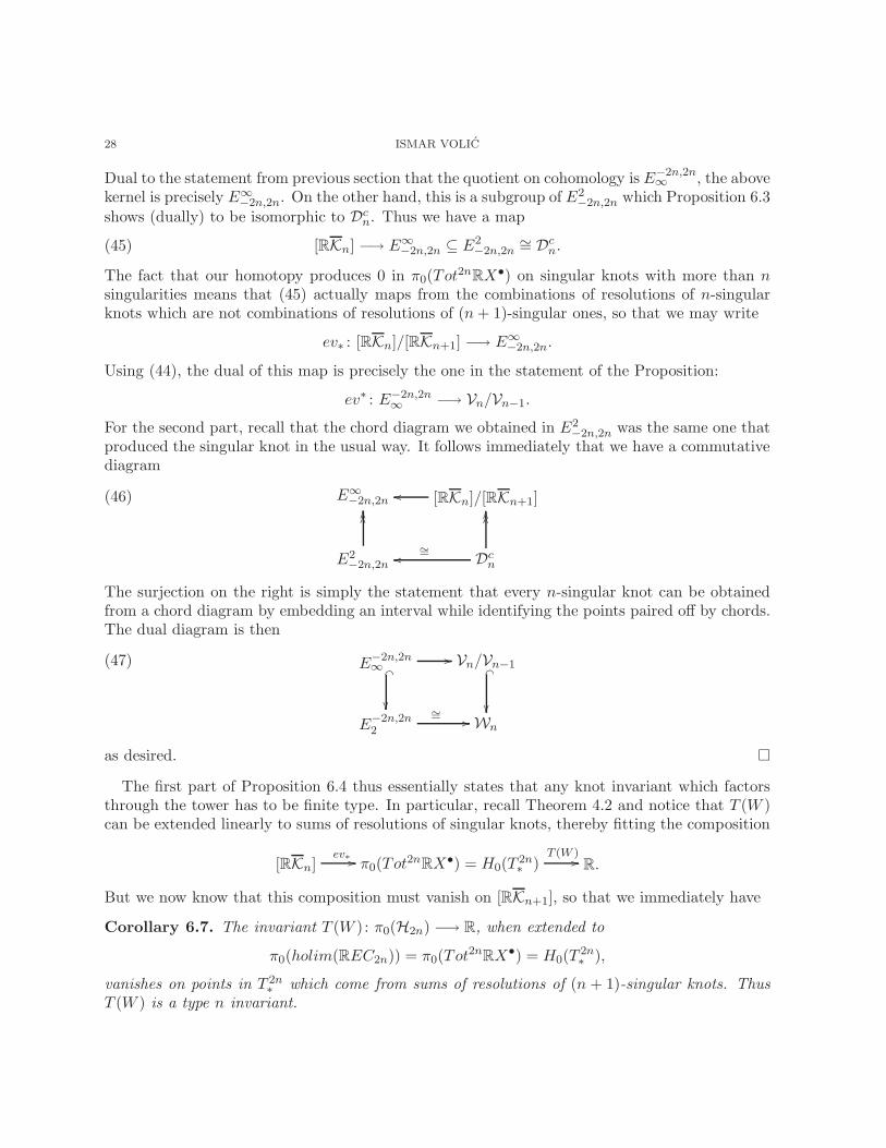
Dual to the statement from previous section that the quotient on cohomology is E−2n,2n∞ , the above

kernel is precisely E∞−2n,2n. On the other hand, this is a subgroup of E2−2n,2n which Proposition 6.3

shows (dually) to be isomorphic to Dcn. Thus we have a map

(45) [RKn] −→ E∞−2n,2n ⊆ E2−2n,2n

∼= Dcn.

The fact that our homotopy produces 0 in π0(Tot2nRX•) on singular knots with more than n

singularities means that (45) actually maps from the combinations of resolutions of n-singularknots which are not combinations of resolutions of (n + 1)-singular ones, so that we may write

ev∗ : [RKn]/[RKn+1] −→ E∞−2n,2n.

Using (44), the dual of this map is precisely the one in the statement of the Proposition:

ev∗ : E−2n,2n∞ −→ Vn/Vn−1.

For the second part, recall that the chord diagram we obtained in E2−2n,2n was the same one that

produced the singular knot in the usual way. It follows immediately that we have a commutativediagram

(46) E∞−2n,2n [RKn]/[RKn+1]oo

E2−2n,2n

OOOO

Dcn

OOOO

∼=oo

The surjection on the right is simply the statement that every n-singular knot can be obtainedfrom a chord diagram by embedding an interval while identifying the points paired off by chords.The dual diagram is then

(47) E−2n,2n∞

// _

Vn/Vn−1 _

E−2n,2n

2

∼= // Wn

as desired.

The first part of Proposition 6.4 thus essentially states that any knot invariant which factorsthrough the tower has to be finite type. In particular, recall Theorem 4.2 and notice that T (W )can be extended linearly to sums of resolutions of singular knots, thereby fitting the composition

[RKn]ev∗ // π0(Tot2n

RX•) = H0(T2n∗ )

T (W )//R.

But we now know that this composition must vanish on [RKn+1], so that we immediately have

Corollary 6.7. The invariant T (W ) : π0(H2n) −→ R, when extended to

π0(holim(REC2n)) = π0(Tot2nRX•) = H0(T

2n∗ ),

vanishes on points in T 2n∗ which come from sums of resolutions of (n + 1)-singular knots. Thus

T (W ) is a type n invariant.


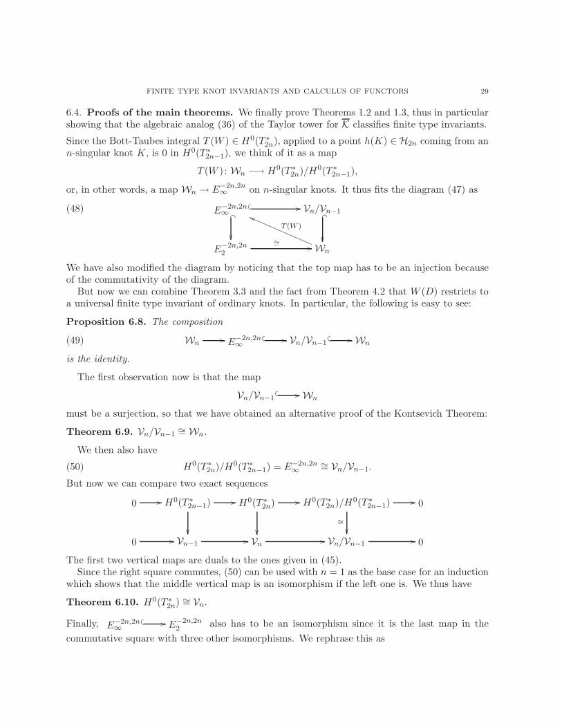
6.4. Proofs of the main theorems. We finally prove Theorems 1.2 and 1.3, thus in particularshowing that the algebraic analog (36) of the Taylor tower for K classifies finite type invariants.

Since the Bott-Taubes integral T (W ) ∈ H0(T ∗2n), applied to a point h(K) ∈ H2n coming from ann-singular knot K, is 0 in H0(T ∗2n−1), we think of it as a map

T (W ) : Wn −→ H0(T ∗2n)/H0(T ∗2n−1),

or, in other words, a map Wn → E−2n,2n∞ on n-singular knots. It thus fits the diagram (47) as

(48) E−2n,2n∞

// _

Vn/Vn−1 _

E−2n,2n

2

∼= // Wn

T (W )

hhQQQQQQQQQQQQQQQ

We have also modified the diagram by noticing that the top map has to be an injection becauseof the commutativity of the diagram.

But now we can combine Theorem 3.3 and the fact from Theorem 4.2 that W (D) restricts toa universal finite type invariant of ordinary knots. In particular, the following is easy to see:

Proposition 6.8. The composition

(49) Wn// E−2n,2n∞

// Vn/Vn−1 // Wn

is the identity.

The first observation now is that the map

Vn/Vn−1 // Wn

must be a surjection, so that we have obtained an alternative proof of the Kontsevich Theorem:


We then also have

(50) H0(T ∗2n)/H0(T ∗2n−1) = E−2n,2n∞

∼= Vn/Vn−1.

But now we can compare two exact sequences

0 // H0(T ∗2n−1)//

H0(T ∗2n) //

H0(T ∗2n)/H0(T ∗2n−1)//

∼=

0

0 // Vn−1// Vn

// Vn/Vn−1// 0

The first two vertical maps are duals to the ones given in (45).Since the right square commutes, (50) can be used with n = 1 as the base case for an induction

which shows that the middle vertical map is an isomorphism if the left one is. We thus have

Theorem 6.10. H0(T ∗2n) ∼= Vn.

Finally, E−2n,2n∞

// E−2n,2n2

also has to be an isomorphism since it is the last map in the

commutative square with three other isomorphisms. We rephrase this as

30 ISMAR VOLIC

Theorem 6.11. The spectral sequence for the cohomology of X• collapses at E2 on the diagonal.

The preceding two results are precisely Theorems 1.2 and 1.3.

6.5. Some further questions. The Taylor tower for K is thus a potentially rich source ofinformation about finite type theory. Its advantage is that the stages Hr lend themselves to purelytopological examination. At the time, not much is known about these spaces, but our results giveevidence that a closer look may shed some light on classical knot theory. In particular:

• For knots in Rn, n > 3, the cohomology spectral sequence is guaranteed to converge to

the totalization of X•. Combining this with the Goodwillie-Klein-Weiss result statingthat in this case the Taylor tower converges to the space of knots, one can extract usefulinformation about the homotopy and cohomology of spaces of knots [28, 23]. However,this may not be true in the case n = 3 because it is not immediately clear that C∗

commutes with totalization. If the spectral sequence indeed does not converge to thedesired associated graded, then potentially an even more interesting question arises: Whatcan we say about invariants pulled back from the Taylor tower without passing to cochainsfirst? It is quite possible that one in this case also obtains only finite type invariants, butthe genuine Taylor tower for K could also contain more information.• Can one gain new insight into finite type theory by studying the homotopy types of spacesHr? In particular, can one gain topological insight into the common thread between knotsin R

3 and Rn, namely the Kontsevich and Bott-Taubes integral constructions of finite type

invariants? This is to be expected, since the latter type of integrals plays a crucial role inour proofs.• What is the relationship between the Taylor tower and Vassiliev’s approach to studyingK through simplicial spaces [30]?• Do other finite type invariants (of homology spheres, for example) also factor through

constructions coming from calculus of functors? One should at least be able to carry theideas and constructions here from knots to braids without too much difficulty.• Can one say anything useful about the inverse limit of the Taylor tower? The question

of invariants of this limit surjecting onto knot invariants is precisely the question of finitetype invariants separating knots.• Recall that the evaluation map ev∗ provides the isomorphism of Theorem 6.10. Budney,

Conant, Scannell, and Sinha [8] examine the evaluation map closely related to ours togive a geometric interpretation of the unique (up to framing) type 2 invariant. Can onein general understand the geometry of finite type invariants using the evaluation map?• As predicted by a result in [16], is the map K→Hr 0-connected, i.e. surjective on π0?

References

[1] D. Altschuler and L. Freidel. On universal Vassiliev invariants. Comm. Math. Phys., 170(1): 41–62, 1995.[2] S. Axelrod and I. Singer. Chern-Simons perturbation theory, II. J. Differential Geom., 39(1): 173–213, 1994.[3] D. Bar-Natan. On the Vassiliev knot invariants. Topology, 34: 423–472, 1995.[4] D. Bar-Natan and A. Stoimenow. The fundamental theorem of Vassiliev invariants. In Lecture Notes in Pure

and Appl. Math., Vol. 184, 1997.[5] R. Bott and C. Taubes. On the self-linking of knots. J. Math. Phys., 35(10): 5247–5287, 1994.[6] A. Bousfield. On the homology spectral sequence of a cosimplicial space. Amer. J. Math., 109(2): 361-394,

1987.


[7] A. Bousfield and D. Kan. Homotopy Limits, Completions, and Localizations. Lecture Notes in Mathematics,Vol. 304, 1972.

[8] R. Budney, J. Conant., K. Scannell, and D. Sinha.New perspectives on self-linking. To appear in Advances in Mathematics.

[9] F. Cohen. The homology of Cn+1 spaces. In Lecture Notes in Mathematics, Vol. 533, 1976.[10] A. Dold. Homology of symmetric products and other functors of complexes. Ann. of Math., 68: 54–80, 1958.[11] A. Dold and R. Thom. Quasifaserungen und unendliche symmetrischen produkte. Ann. of Math., 67: 239–281,

1958.[12] W. Fulton and R. MacPherson. Compactification of configuration spaces. Ann. of Math., 139: 183–225, 1994.[13] T. Goodwillie. Calculus I: The first derivative of pseudoisotopy theory. K-Theory, 4: 1–27, 1990.[14] T. Goodwillie. Calculus II: Analytic functors. K-Theory, 5: 295–332, 1991/92.[15] T. Goodwillie. Calculus III: Taylor series. Geom. Topol., 7: 645-711, 2003.[16] T. Goodwillie and J. Klein. Excision statements for spaces of embeddings. In preparation.[17] T. Goodwillie, J. Klein, and M. Weiss. Spaces of smooth embeddings, disjunction and surgery. Surveys on

Surgery Theory, 2: 221-284, 2001.[18] T. Goodwillie and M. Weiss. Embeddings from the point of view of immersion theory II. Geom. Topol.,

3: 103–118, 1999.[19] A. Hatcher. Algebraic Topology. Cambridge University Press, 2001.[20] D. Kan. Functors involving c.s.s. complexes. Trans. A.M.S., 87: 330–346, 1958.[21] M. Kontsevich. Vassiliev’s knot invariants. Adv. in Sov. Math, 16(2): 137-150, 1993.[22] J. Labastida. Chern-Simons gauge theory: Ten years after. In Trends in theoretical physics, II (Buenos Aires,

1998), AIP Conf. Proc. 484, Amer. Inst. Phys, Woodbury, NY, 1999.[23] P. Lambrechts and I. Volic. On the rational homotopy type of spaces of knots. In preparation.[24] J. P. May. Simplicial Objects in Algebraic Topology. Chicago University Press, 1967.[25] K. Scannell and D. Sinha. A one-dimensional embedding complex. J. Pure Appl. Algebra, 170(1): 93–107,

2002.[26] D. Sinha. Hochschild cohomology of operads and knot spaces. In preparation. Available at

http://math.uoregon.edu/˜dps/respage.html.[27] D. Sinha. Manifold-theoretic compactifications of configuration spaces. To appear in Selecta Mathematica.

[28] D. Sinha. The topology of spaces of knots. Submitted. math.AT/0202287, 2002.[29] D. Thurston. Integral Expressions for the Vassiliev Knot Invariants. Senior Thesis, Harvard University, 1995.[30] V. Vassiliev. Complements of discriminants of smooth maps: topology and applications. Translations of Math-

ematical Monogrphs, Vol. 98, American Mathematical Society, Providence, RI, 1992.[31] I. Volic. Configuration space integrals and Taylor towers for spaces of knots. To appear in Algeb. Geom.

Topol.

[32] M. Weiss. Embeddings from the point of view of immersion theory I. Geom. Topol., 3: 67–101, 1999.

Department of Mathematics, University of Virginia, Charlottesville, VA

E-mail address: [email protected]

URL: http://www.people.virginia.edu/~iv2n

Documents

Introduction K R - palmer.wellesley.edupalmer.wellesley.edu/~ivolic/pdf/Papers/ThesisPaperMaster2.pdf · There are canonical maps K→Hr and Hr →Hr−1, ... The sign convention