- 36 -

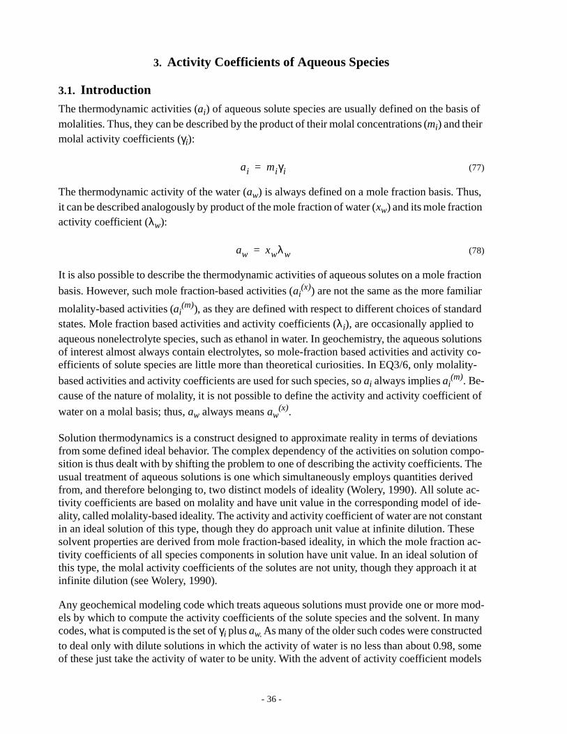
3. Activity Coefficients of Aqueous Species

3.1. IntroductionThe thermodynamic activities (ai) of aqueous solute species are usually defined on the basis of molalities. Thus, they can be described by the product of their molal concentrations (mi) and their molal activity coefficients (γi):

(77)

The thermodynamic activity of the water (aw) is always defined on a mole fraction basis. Thus, it can be described analogously by product of the mole fraction of water (xw) and its mole fraction activity coefficient (λw):

(78)

It is also possible to describe the thermodynamic activities of aqueous solutes on a mole fraction

basis. However, such mole fraction-based activities (ai(x)) are not the same as the more familiar

molality-based activities (ai(m)), as they are defined with respect to different choices of standard

states. Mole fraction based activities and activity coefficients (λi), are occasionally applied to aqueous nonelectrolyte species, such as ethanol in water. In geochemistry, the aqueous solutions of interest almost always contain electrolytes, so mole-fraction based activities and activity co-efficients of solute species are little more than theoretical curiosities. In EQ3/6, only molality-

based activities and activity coefficients are used for such species, so ai always implies ai(m). Be-

cause of the nature of molality, it is not possible to define the activity and activity coefficient of

water on a molal basis; thus, aw always means aw(x).

Solution thermodynamics is a construct designed to approximate reality in terms of deviations from some defined ideal behavior. The complex dependency of the activities on solution compo-sition is thus dealt with by shifting the problem to one of describing the activity coefficients. The usual treatment of aqueous solutions is one which simultaneously employs quantities derived from, and therefore belonging to, two distinct models of ideality (Wolery, 1990). All solute ac-tivity coefficients are based on molality and have unit value in the corresponding model of ide-ality, called molality-based ideality. The activity and activity coefficient of water are not constant in an ideal solution of this type, though they do approach unit value at infinite dilution. These solvent properties are derived from mole fraction-based ideality, in which the mole fraction ac-tivity coefficients of all species components in solution have unit value. In an ideal solution of this type, the molal activity coefficients of the solutes are not unity, though they approach it at infinite dilution (see Wolery, 1990).

Any geochemical modeling code which treats aqueous solutions must provide one or more mod-els by which to compute the activity coefficients of the solute species and the solvent. In many codes, what is computed is the set of γi plus aw. As many of the older such codes were constructed to deal only with dilute solutions in which the activity of water is no less than about 0.98, some of these just take the activity of water to be unity. With the advent of activity coefficient models

ai miγi=

aw xwλw=

- 37 -

of practical usage in concentrated solutions (mostly based on Pitzer’s 1973, 1975 equations), there has been a movement away from this particular and severe approximation. Nevertheless, it is generally the activity of water, rather than the activity coefficient of water, which is evaluated from the model equations. This is what was previously done in EQ3/6. However, EQ3/6 now evaluates the set of γi plus λw. This is done to avoid possible computational singularities that may arise, for example if heterogeneous equilibria happen to fix the activity of water (e.g., when a solution is saturated with both gypsum and anhydrite).

Good models for activity coefficients must be accurate. A prerequisite for general accuracy is thermodynamic consistency. The activity coefficient of each aqueous species is not independent of that of any of the others. Each is related to a corresponding partial derivative of the excess

Gibbs energy of the solution (GEX). The excess Gibbs energy is the difference between the com-plete Gibbs energy and the ideal Gibbs energy. Because there are two models of ideality, hence

two models for the ideal Gibbs energy, there are two forms of the excess Gibbs energy, GEXm

(molality-based) and GEXx (mole fraction-based). The consequences of this are discussed by Wolery (1990). In version 7.0 of EQ3/6, all activity coefficient models are based on ideality de-

fined in terms of molality. Thus, the excess Gibbs energy of concern is GEXm. The activity of wa-ter, which is based on mole-fraction ideality, is imported into this structure as discussed by Wolery (1990). The relevant differential equations are:

(79)

(80)

where R is the gas constant, T the absolute temperature, Ω the number of moles of solvent water comprising a mass of 1 kg (Ω ≈ 55.51),and:

(81)

the sum of molalities of all solute species. Given an expression for the excess Gibbs energy, such equations give a guaranteed route to thermodynamically consistent results (Pitzer, 1984; Wolery, 1990). Equations that are derived by other routes may be tested for consistency using other rela-tions, such as the following forms of the cross-differentiation rule (Wolery, 1990):

(82)

(83)

ln γi1

RT------- G

EXm∂ni∂

-----------------=

ln awΣmΩ

--------–1

RT------- G

EXm∂nw∂

-----------------+=

Σm mii

∑=

ln γj∂mi∂

--------------lnγi∂mj∂

-------------=

ln aw∂ni∂

----------------ln γi∂nw∂

-------------- 1nw------–=

- 38 -

In general, such equations are most easily used to prove that a set of model equations is not ther-modynamically consistent. The issue of sufficiency in proving consistency using these and relat-ed equations (Gibbs-Duhem equations and sum rules) is addressed by Wolery (1990).

The activity coefficients in reality are complex functions of the composition of the aqueous so-lution. In electrolyte solutions, the activity coefficients are influenced mainly by electrical inter-actions. Much of their behavior can be correlated in terms of the ionic strength, defined by:

(84)

where the summation is over all aqueous solute species and zi is the electrical charge. However, the use of the ionic strength as a means of correlating and predicting activity coefficients has been taken to unrealistic extremes (e.g., in the mean salt method of Garrels and Christ, 1965, p. 58-60). In general, model equations which express the dependence of activity coefficients on solu-tion composition only in terms of the ionic strength are restricted in applicability to dilute solu-tions.

The three basic options for computing the activity coefficients of aqueous species in EQ3/6 are models based respectively on the Davies (1962) equation, the “B-dot” equation of Helgeson (1969), and Pitzer’s (1973, 1975, 1979, 1987) equations. The first two models, owing to limita-tions on accuracy, are only useful in dilute solutions (up to ionic strengths of 1 molal at most). The third basic model is useful in highly concentrated as well as dilute solutions, but is limited in terms of the components that can be treated.

With regard to temperature and pressure dependence, all of the following models are parameter-ized along the 1 atm/steam saturation curve. This corresponds to the way in which the tempera-ture and pressure dependence of standard state thermodynamic data are also presently treated in the software. The pressure is thus a function of the temperature rather than an independent vari-able, being fixed at 1.013 bar from 0-100°C and the pressure for steam/liquid water equilibrium from 100-300°C. However, some of the data files have more limited temperature ranges.

3.2. The Davies EquationThe first activity coefficient model in EQ3/6 is based on the Davies (1962) equation:

(85)

(the constant 0.2 is sometimes also taken as 0.3). This is a simple extended Debye-Hückel model (it reduces to a simple Debye-Hückel model if the “0.2I” part is removed). The Davies equation is frequently used in geochemical modeling (e.g., Parkhurst, Plummer, and Thorstenson, 1980; Stumm and Morgan, 1981). Note that it expresses all dependence on the solution composition through the ionic strength. Also, the activity coefficient is given in terms of the base ten loga-rithm, instead of the natural logarithm. The Debye-Hückel Aγ parameter bears the additional label “10” to ensure consistency with this. The Davies equation is normally only used for temperatures close to 25°C. It is only accurate up to ionic strengths of a few tenths molal in most solutions. In

I12--- mizi

2

i

∑=

γilog Aγ 10, zi2 I

1 I+--------------- 0.2I+

–=

- 39 -

some solutions, inaccuracy, defined as the condition of model results differing from experimental measurements by more than the experimental error, is apparent at even lower concentrations.

In EQ3/6, the Davies equation option is selected by setting the option flag iopg1 = -1. A support-ing data file consistent with the use of a simple extended Debye-Hückel model must also be sup-plied (e.g., data1 = data1.com, data1.sup, or data1.nea). If iopg1 = -1 and the supporting data file is not of the appropriate type, the software terminates with an error message.

The Davies equation has one great strength: the only species-specific parameter required is the electrical charge. This equation may therefore readily be applied to a wide spectrum of species, both those whose existence is well-established and those whose existence is only hypothetical.

The Davies equation predicts a unit activity coefficient for all neutral solute species. This is known to be inaccurate. In general, the activity coefficients of neutral species that are non-polar (such as O2(aq), H2(aq), and N2(aq)) increase with increasing ionic strength (the “salting out ef-fect,” so named in reference to the corresponding decreasing solubilities of such species as the salt concentration is increased; cf. Garrels and Christ, 1965, p. 67-70). In addition, Reardon and Langmuir (1976) have shown that the activity coefficients of two polar neutral species (the ion pairs CaSO4(aq) and MgSO4(aq)) decrease with increasing ionic strength, presumably as a conse-quence of dipole-ion interactions.

The Davies equation is thermodynamically consistent. It is easy to show, for example, that it sat-isfies the solute-solute form of the cross-differentiation equation.

Most computer codes using the Davies equation set the activity of water to one of the following: unity, the mole fraction of water, or a limiting expression for the mole fraction of water. Usage of any of these violates thermodynamic consistency, but this is probably not of great significance as the inconsistency is numerically not significant at the relatively low concentrations at which the Davies equation itself is accurate. For usage in EQ3/6, we have used standard thermodynamic relations to derive the following expression:

(86)

where “2.303” is a symbol for and approximation of ln 10 (warning: this is not in general a suf-ficiently accurate approximation) and:

(87)

This result is thermodynamically consistent with the Davies equation.

3.3. The B-dot EquationThe second model for activity coefficients available in EQ3/6 is based on the B-dot equation of Helgeson (1969) for electrically charged species:

awlog1Ω---- Σm

2.303-------------–

23---Aγ 10, I

32---

σ I( ) 2 0.2( )Aγ 10, I2

–+

=

σ x( ) 3

x3

----- 1 x1

1 x+------------– 2 ln 1 x+( )–+

=

- 40 -

(88)

Here åi is the hard core diameter of the species, Bγ is the Debye-Hückel B parameter, and is the characteristic B-dot parameter. Like the Davies equation, this is a simple extended Debye-

Hückel model, the extension being the “ I” term. The Debye-Hückel part of this equation is equivalent to that of the Davies equation if the product “åiBγ” has a value of unity. In the extend-

ed part, these equations differ in that the Davies equation has a coefficient in place of which depends on the electrical charge of the species in question.

In EQ3/6, the B-dot equation option is selected by setting the option flag iopg1 = 0. A supporting data file consistent with the use of a simple extended Debye-Hückel model must also be supplied (e.g., data1 = data1.com, data1.sup, or data1.nea). Note that these data files support the use of the Davies equation as well (the åi data on these files is simply ignored in that case). If iopg1 = 0 and the supporting data file is not of the appropriate type, the software terminates with an error message.

The B-dot equation has about the same level of accuracy as the Davies equation, and almost as much universality (one needs to know åi in addition to zi). However, it fails to satisfy the solute-solute form of the cross-differentiation rule. The first term is consistent with this rule only if all hard core diameters have the same value. The second is consistent only if all ions share the same value of the square of the electrical charge. However, the numerical significance of the inconsis-tency is small in the range of low concentrations in which this equation can be applied with useful accuracy. On the positive side, the B-dot equation has been developed (Helgeson, 1969) to span a wide range of temperature (up to 300°C).

For electrically neutral solute species, the B-dot equation reduces to:

(89)

As has positive values at all temperatures in the range of application, the equation predicts a salting out effect. However, by tradition (Helgeson et al., 1970), the B-dot equation itself is not used in the case of neutral solute species. The practice, as suggested by Garrels and Thompson (1962) and reiterated by Helgeson (1969), is to assign the value of the activity coefficient of aqueous CO2 in otherwise pure sodium chloride solutions of the same ionic strength. This func-tion was represented in previous versions of EQ3/6 by a power series in the ionic strength:

(90)

The first term on the right hand side dominates the others. The first coefficient is positive, so the activity coefficient of CO2 increases with increasing ionic strength (consistent with the “salting out” effect). As it was applied in EQ3/6, the coefficients for the power series themselves were represented as similar power series in temperature, and this model was fit to data taken from Ta-

γilogAγ 10, zi

2I

1 åiBγ I+--------------------------– B· I+=

B·

B·

B·

γilog B· I=

B·

γilog k1I k2I2

k3I3

k4I4

+ + +=

- 41 -

ble 2 of Helgeson (1969). These data (including extrapolations made by Helgeson) covered the range 25-300°C and 0-3 molal NaCl.

The high order power series in eq (90) was unfortunately very unstable when extrapolated out-side the range of the data to which it was fit. EQ3NR and EQ6 would occasionally run into an unrecoverable problem attempting to evaluate this model for high ionic strength values generated in the process of attempting to find a numerical solution (not necessarily because the solutions in question really had high ionic strength). To eliminate this problem, the high order power series has been replaced by a new expression after Drummond (1981, p. 19):

(91)

where T is the absolute temperature and C = -1.0312, F = 0.0012806, G = 255.9, E = 0.4445, and H = -0.001606. Note that this is presented in terms of the natural logarithm. Conversion is ac-complished by using the relation:

(92)

This expression is both much simpler (considering the dependencies on both temperature and ionic strength) and is more stable. However, in deriving it, the ionic strength was taken to be equivalent to the sodium chloride molality. In the original model (based on Helgeson, 1969), the ionic strength was based on correcting the sodium chloride molality for ion pairing. This correc-tion is numerically insignificant at low temperature. It does become significant at high tempera-ture. However, neither this expression nor the power series formulation it replaced is thermodynamically consistent with the B-dot equation itself, as can be shown by applying the solute-solute cross-differentiation rule.

The more recent previous versions of EQ3/6 only applied the “CO2” approximation to species that are essentially nonpolar (e.g., O2(aq), H2(aq), N2(aq)), for which salting-out would be expect-ed. In the case of polar neutral aqueous species, the activity coefficients were set to unity (fol-lowing the recommendation of Garrels and Christ, 1965, p. 70); i.e., one has:

(93)

This practice is still followed in the present version of the code.

EQ3/6 formerly complemented the B-dot equation with an approximation for the activity of wa-ter that was based on assigning values in pure sodium chloride solutions of the same “stoichio-metric” ionic strength (Helgeson et al., 1970). This approximation was fairly complex and was, of course, not thermodynamically consistent with the B-dot equation itself. In order to simplify the data requirements, as well as avoid the need to employ a second ionic strength function, this

formulation has been replaced by a new one which depends on the parameter and is quasi-con-sistent with the B-dot equation:

lnγi C FTGT----+ +

I E HT+( ) II 1+-----------

–=

xlogln x

2.303-------------=

γilog 0=

B·

- 42 -

(94)

The solute hard core diameter (å) is assigned a fixed value of 4.0Å (a reasonable value). This equation is consistent with the B-dot equation if all solute species are ions, have the same fixed value of the hard core diameter, and have the same value of the square of the electrical charge.

3.4. Scaling of Individual Ionic Activity Coefficients: pH ScalesBefore proceeding to a discussion of Pitzer’s (1973, 1975) equations, we will address the prob-lem of scaling associated with the activity coefficients of individual ions. It is not possible to ob-serve (measure) any of the thermodynamic functions of such species, because any real solution must be electrically balanced. Thus, the activity coefficients of aqueous ions can only be mea-sured in electrically neutral combinations. These are usually expressed as the mean activity co-efficients of neutral electrolytes. The mean activity coefficient of neutral electrolyte MX (M denoting the cation, X the anion) is given by:

(95)

where νM is the number of moles of cation produced by dissociation of one mole of the electro-lyte, νX is the number of moles of anion produced, and:

(96)

Electrical neutrality requires that:

(97)

Although the activity coefficients of ions can not be individually observed, the corresponding molal concentrations can be. The corresponding products, the thermodynamic activities of the ions, are not individually observable, precisely because of the problem with the activity coeffi-cients. Thus, the problem of obtaining individual activity coefficients of the ions and the problem of obtaining individual activities of the same species is really the same problem.

Individual ionic activity coefficients can be defined on a conventional basis by introducing some arbitrary choice. This is can be made by adopting some expression for the activity coefficient of a single ion. The activity coefficients of all other ions then follow via electroneutrality relations. The activities for all the ions are then also determined (cf. Bates and Alfenaar, 1969). Because this applies to the hydrogen ion, such an arbitrary choice then determines the pH. Such conven-tions are usually made precisely for this purpose, and they are generally known as pH scales.The NBS pH scale, which is the basis of nearly all modern conventional pH measurement, is based on the Bates-Guggenheim equation (Bates, 1964):

awlog1Ω---- Σm

2.303-------------–

23---Aγ 10, I

32---

σ åBγ I( ) B· I2

–+

=

γ ,MX±logνM γMlog νX γXlog+

νMX--------------------------------------------------=

νMX νM νX+=

zMνM zXνX–=

- 43 -

(98)

This scale is significant not only to the measurement of pH, but of corresponding quantities (e.g., pCl, pBr, pNa) obtained using other specific-ion electrodes (cf. Bates and Alfenaar, 1969; Bates, 1973; Bates and Robinson, 1974).

The Bates-Guggenheim equation, like the Davies equation and the B-dot equation, is an extended Debye-Hückel formula. However, if one applies the Davies equation or the B-dot equation to the chloride ion, the result is not precisely identical. The difference approaches zero as the ionic strength approaches zero, and is not very significant quantitatively in the low range of ionic strength in which either the Davies equation or the B-dot equation has useful accuracy. Never-theless, the use of either of these equations in uncorrected form introduces an inconsistency with measured pH values, as use of the Davies equation for example would interpret the pH as being on an implied “Davies” scale.

Activity coefficients (and activities) of ions can be moved from one scale to another. The general relation for converting from scale (1) to scale (2) is (Knauss, Wolery, and Jackson, 1991):

(99)

For example, if we evaluate the Davies equation for all ions, we may take the results as being on scale (1). To convert these to the NBS scale (here scale (2)), we take the j-th ion to be the chloride ion and evaluate the Bates-Guggenheim equation. We then apply the scale conversion equation to every other ion i.

In EQ3/6, activity coefficients are first calculated from the “raw” single-ion equations. They are then immediately rescaled, unless no rescaling is to be done. Thus, rescaling occurs during the iteration process; it is not deferred until convergence has been achieved. The user has control over rescaling via the option switch iopg2. If iopg2 = 0, all single-ion activity coefficients and activities are put on the NBS scale. If iopg2 = -1, no rescaling is performed. If iopg2 = 1, all sin-gle-ion activity coefficients and activities are put on a scale which is defined by the relation:

(100)

This has the effect of making the activity and the molality of the hydrogen ion numerically equal. This may have some advantages in comparing with experimental measurements of the hydrogen ion molality. Such measurement techniques have recently been discussed by Mesmer (1991).

The problem of scaling the activity coefficients of ions is more acute in concentrated solutions, and the need to discriminate among different scales in geochemical modeling codes has only been addressed as such codes have been written or modified to treat such solutions (e.g., Harvie, Møller, and Weare, 1984; Plummer et al., 1988).

γCl-

logA– γ 10, I

1 1.5 I+-----------------------=

γi2( )

log γi1( )

logzi

zj--- γj

2( )log γj

1( )log–( )= =

γH+log 0=

- 44 -

3.5. Pitzer’s Equations

3.5.1. IntroductionPitzer (1973, 1975) proposed a set of semi-empirical equations to describe activity coefficients in aqueous electrolytes. These equations have proven to be highly successful as a means of deal-ing with the thermodynamics of concentrated solutions (e.g., Pitzer and Kim, 1974). Models based on these equations have been developed to describe not only solution properties, but also equilibrium between such solutions and salt minerals (e.g., Harvie and Weare, 1980; Harvie, Møller, and Weare, 1984). The utility of these models in geochemical studies has been well es-tablished. For example, such models have been shown to account for the mineral sequences pro-duced by evaporation of seawater (Harvie et al., 1980), the process of trona deposition in Lake Magadi, Kenya (Monnin and Schott, 1984), and the formation of the borate-rich evaporite depos-its at Searles Lake, California (Felmy and Weare, 1986).

Pitzer’s equations are based on a semi-theoretical (see Pitzer, 1973) interpretation of ionic inter-actions, and are written in terms of interaction coefficients (and parameters from which such co-efficients are calculated). There are two main categories of such coefficients, “primitive” ones which appear in the original theoretical equations, but most of which are only observable in cer-tain combinations, and others which are “observable” by virtue of corresponding to observable combinations of the primitive coefficients or by virtue of certain arbitrary conventions. Only the observable coefficients are reported in the literature.

There is a very extensive literature dealing with Pitzer’s equations and their application in both interpretation of experimental data and calculational modeling. A complete review is beyond the scope of the present manual. Discussion here will be limited to the equations themselves, how to use them in EQ3/6, and certain salient points that are necessary in order to use them in an in-formed manner. Readers who wish to pursue the subject further are referred to reviews given by Pitzer (1979, 1987, 1992). Jackson (1988) has addressed the verification of the addition of Pitzer’s equations to EQ3/6.

In EQ3/6, the Pitzer’s equations option is selected by setting the option flag iopg1 = 1. A sup-porting data file consistent with this option must also be supplied (e.g., data1 = data1.hmw or data1.pit). If iopg1 = 1 and the supporting data file is not of the appropriate type, the software terminates with an error message.

Pitzer’s equations are based on the following virial expansion for the excess Gibbs energy:

(101)

where ww is the number of kilograms of solvent water, f(I) is a Debye-Hückel function describ-ing the long-range electrical interactions to first order, the subscripts i, j, and k denote aqueous solute species, and ni is the number of moles of the i-th solute species. The equation also contains two kinds of interaction or virial coefficients: the λij are second order interaction coefficients, and the µijk are third order interaction coefficients. A key element in the success of Pitzer’s equations is the treatment of the second order interaction coefficients as functions of ionic strength. As will

GEXm

RT wwf I( ) 1ww-------

λij I( )ninji j

∑ 1

ww2

-------

µijkninjnki j k

∑+ +

=

- 45 -

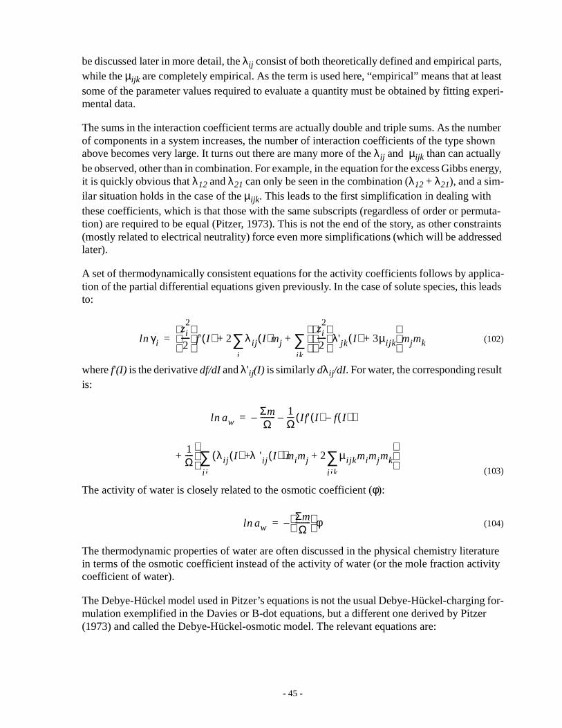
be discussed later in more detail, the λij consist of both theoretically defined and empirical parts, while the µijk are completely empirical. As the term is used here, “empirical” means that at least some of the parameter values required to evaluate a quantity must be obtained by fitting experi-mental data.

The sums in the interaction coefficient terms are actually double and triple sums. As the number of components in a system increases, the number of interaction coefficients of the type shown above becomes very large. It turns out there are many more of the λij and µijk than can actually be observed, other than in combination. For example, in the equation for the excess Gibbs energy, it is quickly obvious that λ12 and λ21 can only be seen in the combination (λ12 + λ21), and a sim-ilar situation holds in the case of the µijk. This leads to the first simplification in dealing with these coefficients, which is that those with the same subscripts (regardless of order or permuta-tion) are required to be equal (Pitzer, 1973). This is not the end of the story, as other constraints (mostly related to electrical neutrality) force even more simplifications (which will be addressed later).

A set of thermodynamically consistent equations for the activity coefficients follows by applica-tion of the partial differential equations given previously. In the case of solute species, this leads to:

(102)

where f'(I) is the derivative df/dI and λ'ij(I) is similarly dλij/dI. For water, the corresponding result is:

(103)

The activity of water is closely related to the osmotic coefficient (φ):

(104)

The thermodynamic properties of water are often discussed in the physical chemistry literature in terms of the osmotic coefficient instead of the activity of water (or the mole fraction activity coefficient of water).

The Debye-Hückel model used in Pitzer’s equations is not the usual Debye-Hückel-charging for-mulation exemplified in the Davies or B-dot equations, but a different one derived by Pitzer (1973) and called the Debye-Hückel-osmotic model. The relevant equations are:

ln γi

zi2

2-----

f' I( ) 2 λij I( )mjj

∑zi2

2-----

λ'jk I( ) 3µijk+

mjmkjk

∑+ +=

ln awΣmΩ

--------–1Ω---- If ' I( ) f I( )–( )–=

1Ω---- λij I( ) λ'ij I( )+( )mimj

i j

∑ 2 µijkmimjmki jk

∑+

+

ln awΣmΩ

-------- φ–=

- 46 -

(105)

(106)

The Debye-Hückel parameter Aφ is related to the more familiar Aγ,10 by:

(107)

The parameter b is assigned a constant value of 1.2 (Pitzer, 1973). Theoretically, this is the prod-uct åBγ; thus the hard core diameter at 25°C is effectively fixed at a value of about 3.65Å (and somewhat different values at other temperatures). Differences in the hard core diameters of var-ious ions in solution are not explicitly accounted for (this is the case also in the Davies equation). However, the interaction coefficient terms of the equation effectively compensate for this. A very important feature of the Debye-Hückel-osmotic model is that it, like the Debye-Hückel-charging model, is consistent with the Debye-Hückel limiting law:

(108)

3.5.2. Solutions of ElectrolytesIn a pure solution of aqueous neutral electrolyte MX, the following combinations of interaction coefficients are observable:

(109)

(110)

For example, the osmotic coefficient for such a solution can be written in the form (Pitzer, 1973):

(111)

Appearing in this equation is , which is given by:

f I( )4AφI

b------------

ln 1 b I+( )–=

f' I( ) 2Aφ2b--- ln 1 b I+( ) I

1 b I+( )-----------------------+

–=

Aφ2.303Aγ 10,

3---------------------------=

γilog Aγ 10, zi2

I as–→ I 0→

BMX I( ) λMX I( )zX

2zM---------- λMM I( )

zM

2zX-------- λXX I( )+ +=

CMXφ

3zX

zM------

12---

µMMXzM

zX------

12---

µMXX+

=

φ 1–zMzX

2--------------- If' I( ) f I( )–( )=

2νMνX

νMX-----------------

BMXφ

I( )mMX

2 νMνX( )32---

νMX-------------------------

CMXφ

mMX2

+ +

BMXφ

- 47 -

(112)

Here B'MX(I) is the derivative of BMX(I) with respect to the ionic strength.

The ionic strength dependence of was defined by Pitzer (1973) to take the following form:

(113)

where α was assigned a constant value of 2.0. and , along with , are parameters

whose values are determined by fitting experimental data, such as for the osmotic coefficient. Corresponding to the above equation is:

(114)

where:

(115)

Pitzer and Mayorga (1974) proposed a description for in the case of 2:2 electrolytes that is

based on an additional fitting parameter:

(116)

Here α1 is assigned a value of 1.4 and α2 one of 12.0 and is the additional fitting parameter.

Corresponding to this is:

(117)

We consider first the exponential function in eqs (113) and (117). This is shown in Figure 2 for the three commonly used values of α. At zero ionic strength, this function has a value of unity.

Thus, or . The magnitude of each term con-

taining or decreases exponentially as the ionic strength increases, approaching zero

as the ionic strength approaches infinity (a limit which is not of physical interest). Most of the

decay takes place in the very low ionic strength range. Thus, the terms in and are im-

portant parts of the model, even in dilute solutions.

BMXφ

I( ) BMX I( ) IB'MX I( )+=

BMXφ

BMXφ

I( ) βMX0( ) βMX

1( )e

α I–+=

βMX0( ) βMX

1( )CMX

φ

BMX I( ) βMX0( ) βMX

1( )g α I( )+=

g x( ) 2

x2

----- 1 1 x+( )e x–

–( )=

BMXφ

BMXφ

I( ) βMX0( ) βMX

1( )e

α1 I–βMX

2( )e

α2 I–+ +=

βMX2( )

BMX I( ) βMX0( ) βMX

1( )g α1 I( ) βMX

2( )g α2 I( )+ +=

BMXφ βMX

0( ) βMX1( )

+= BMXφ βMX

0( ) βMX1( ) βMX

2( )+ +=

βMX1( ) βMX

2( )

βMX1( ) βMX

2( )

- 48 -

The function g(x) is shown in Figure 3 for the three commonly used α values. It resembles the above exponential function, though it does not decay quite so rapidly. This function may be ex-panded as follows:

(118)

This shows that g(x) = 1 at x = 0 (I = 0). Thus, at zero ionic strength, or

. It can be shown that g(x) approaches zero as x (and I) approach in-

finity.

The development thus far shows that there are two major categories of interaction coefficients. The λij and the µijk in terms of which the theoretical equations were originally derived are what we will call the primitive interaction coefficients. The observable combinations of these, such as

, , , and , are what we will call the observable interaction coefficients. This

latter kind of interaction coefficient represents the model data that are reported for the various systems for which Pitzer’s equations have been fit to experimental data.

I

exp(

-α-/

I)

0 1 2 3 4 5 60.0

0.2

0.4

0.6

0.8

1.0

α = 2.0α = 1.4α = 12.0

Figure 2. Behavior of the exponential function governing the ionic strength dependence of second-orderinteractions among cations and anions.

exp(

- α√I

)

g x( ) 1 22x3!------ 3x

4!------–

4x2

5!-------- 5x

3

6!--------– ...+ +

–=

BMX βMX0( ) βMX

1( )+=

BMX βMX0( ) βMX

1( ) βMX2( )

+ +=

βMX0( ) βMX

1( ) βMX2( )

CMXφ

- 49 -

It is possible to rewrite the equations for ln γi and ln aw in complex mixtures in terms of the ob-servable interaction coefficients. An example of such equations was suggested by Pitzer (1979) and adopted with changes in notation by Harvie, Møller, and Weare (1984). These equations are much more complex than the original form written in terms of the primitive interaction coeffi-cients. They have been incorporated into computer codes, such as that of Harvie, Møller, and Weare (1984), PHRQPITZ (Plummer et al., 1988), and SOLMINEQ.88 (Perkins et al., 1990). As noted in the previous section, there is no unique way to construct equations for single-ion activity coefficients. Furthermore, direct usage of such equations constitutes implicit adoption of a cor-responding pH scale. In the case of the single-ion activity coefficient equation suggested by Pitzer, this could be termed the “Pitzer” scale.

The equations for ln γi and ln aw which are evaluated in EQ3/6 are those written in terms of the primitive interaction coefficients. The set of these which is used is not the generalized theoretical set, which is not obtainable for the reasons discussed previously, but a practical set that is ob-tained by mapping the set of reported observable interaction coefficients using a set of equations that contain arbitrary conventions. These mapping equations imply a pH scale. We will show that the conventions chosen here match those suggested by Pitzer (1979), so this implied pH scale is identical to his.

The basic guides to choosing such mapping conventions are pleasing symmetries and the desir-ability of minimizing the number of conventional primitive interaction coefficients with non-zero values. In the case of the second order coefficients, both of these considerations suggest the following definitions:

I

g(α-

/I)

0 1 2 3 4 5 60.0

0.2

0.4

0.6

0.8

1.0

α = 2.0α = 1.4α = 12.0

Figure 3. Behavior of the g(x) function governing the ionic strength dependence of second-order interactions among cations and anions.

g(α√

I)

- 50 -

(119)

(120)

(121)

Analogous to the formulas used to describe , one may write:

(122)

or:

(123)

From the principle of corresponding terms, it follows that the corresponding mapping equations are:

(124)

(125)

(126)

Evaluation of the equations for ln γi and ln aw also requires the ionic strength derivatives of the λij coefficients. These are given by:

(127)

or:

(128)

where g'(x) is the derivative of g(x) (with respect to x, not I), given by

(129)

The principle of pleasing symmetry suggests the following mapping equations for dealing with

the parameter:

λMM I( ) 0=

λXX I( ) 0=

λMX I( ) BMX I( )=

BMX

λMX I( ) λMX0( ) λMX

1( )g α I( )+=

λMX I( ) λMX0( ) λMX

1( )g α1 I( ) λMX

2( )g α2 I( )+ +=

λMMn( )

0 for n = 0, 2=

λXXn( )

0 for n = 0, 2=

λMXn( ) βMX

n( )for n = 0, 2=

λ'MX I( ) λMX1( )

g' x( ) α2 I---------

=

λ'MX I( ) λMX1( )

g' x( )α1

2 I---------

λMX2( )

g' x( )α2

2 I---------

+=

g' x( ) 4

x3

----- 1 e

x–1 x

x2

2-----+ +

– –=

CMXφ

- 51 -

(130)

(131)

The two µ coefficients are then related by:

(132)

These are in fact the mapping equations used in EQ3/6. However, the principle of minimizing the number of conventional primitive interaction coefficients would suggest instead mapping re-lations such as:

(133)

(134)

Note that with this set of mapping relations, a different pH scale would be implied.

In mixtures of aqueous electrolytes with a common ion, two additional observable combinations of interaction coefficients appear (Pitzer, 1973; Pitzer and Kim, 1974):

(135)

and:

(136)

Here M and M' are two cations and X is the anion, or M and M' are two anions and X is the cation. From previously adopted mapping conventions, it immediately follows that the corresponding mappings are given by:

(137)

(138)

µMMX16---

zM

zX------

12---

CMXφ

=

µMXX16---

zX

zM------

12---

CMXφ

=

µMMX

zM---------------

µMXX

zX--------------=

µMMX13---

zM

zX------

12---

CMXφ

=

µMXX 0=

θMM' I( ) λMM' I( )zM'

2zM----------

λMM I( )–zM

2zM'----------

λM'M' I( )–=

ψMM'X 6µMM'X

3zM'

zM----------

µMMX–3zM

zM'----------

µM'M'X–=

λMM' I( ) θMM' I( )=

µMM'X16--- ψMM'X

3zM'

zM----------

µMMX

3zM

zM'----------

µM'M'X+ +

=

- 52 -

In the original formulation of Pitzer’s equations (Pitzer, 1973), the θMM' coefficient is treated as a constant. It was later modified by Pitzer (1975) to take the following form:

(139)

corresponds to the of Harvie, Møller, and Weare (1984). The first term is a con-

stant and accounts for short-range effects (this is the of Harvie, Møller, and Weare). The sec-

ond term, which is the newer part, is entirely theoretical in nature and accounts for higher-order

electrostatic effects. Only the part is obtained by fitting. Corresponding to this is the

equation:

(140)

The relevant mapping relation is then:

(141)

The part is obtainable directly from theory (Pitzer, 1975):

(142)

where:

(143)

in which:

(144)

and:

(145)

The derivative of is given by:

θMM' I( ) SθMM'EθMM' I( )+=

θMM' I( ) Φij

θij

SθMM'

λMM' I( ) SλMM'EλMM' I( )+=

SλMM'SθMM'=

EλMM' I( )

EθMM'zMzM'

4I--------------

J xMM'( )J xMM( )

2-------------------–

J xM'M'( )2

---------------------– =

J x( ) 1x--- 1 q

q2

2----- e

q–+ +

y2dy

0

∞

∫=

qxy--

ey–

–=

xij 6zizjAφ

I=

EλMM' I( )

- 53 -

(146)

Expansion of J(x) gives (Pitzer, 1975):

(147)

Application of L’Hospital’s rule shows that J(x) goes to zero as x goes to zero (hence also as the ionic strength goes to zero). J(x) is a monotonically increasing function. So is J'(x), which ap-proaches a limiting value of 0.25 as x goes to infinity. The function J(x) and its derivative are approximated in EQ3/6 by a Chebyshev polynomial method suggested by Harvie and Weare (1980). This method is described in detail by Harvie (1981, Appendix B, in which J(x) is referred to as J0(x)); this method is also described in the review by Pitzer (1987, p. 131-132).

Pitzer (1979) showed that substitution of the observable interaction coefficients into the single-ion activity coefficient equation gives the following result for cation M:

(148)

Here a denotes anions, c denotes cations, and:

(149)

(150)

(151)

Eλ'MM' I( )Eλ I( )

I--------------

–=

zMzM'

8I2

--------------

xMM'J' xMM'( )xMMJ' xMM( )

2--------------------------------–

xM'M'J' xM'M'( )2

-----------------------------------– +

J x( ) x2

6-----

ln x 0.419711+( )– ...+=

ln γM zM2

fγ

2 ma BMa Σmz( )CMa+[ ]a

∑+ +=

2 mcθMcc

∑ mcma zM2

B'ca zMCca ψMca+ +[ ]a

∑c

∑+ +

12--- mama' zM

2 θ'aa' ψMaa'+[ ]a'

∑a

∑zM2

2------ mcmc'θ'cc'

c'

∑c

∑+ +

zM

mcλcc

zc---------------

c

∑maλaa

za----------------

a

∑–32--- mcma

µcca

zc-----------

µcaa

za-----------–

a

∑c

∑+

fγ f'

2---=

CMX

CMXφ

2 zMzX

-----------------------=

Σmz mcmcc

∑=

- 54 -

(The single-ion equation for an anion is analogous). As pointed out by Pitzer, the unobservability of single-ion activity coefficients in his model lies entirely in the last term (the fourth line) of the equation and involves the primitive interaction coefficients λcc, λaa, µcca, and µcaa. His suggest-ed conventional single-ion activity coefficient equation is obtained by omitting this part. This re-quires the affected primitive interaction coefficients to be treated exactly as in the previously adopted mapping equations. This approach could in fact have been used to derive them.

In theory, the relevant data required to evaluate Pitzer’s equations for complex mixtures of rela-tively strong aqueous electrolytes can all be obtained from measurements of the properties of

pure aqueous electrolytes (giving the observable interaction coefficients , , , and

) and mixtures of two aqueous electrolytes having a common ion ( and ).

There is one peculiarity in this fitting scheme in that is obtainable from more than one

mixture of two electrolytes having a common ion, because this parameter does not in theory de-pend on that ion. Thus, the value adopted may have to be arrived at by simultaneously consider-ing the experimental data for a suite of such mixtures.

3.5.3. Solutions of Electrolytes and NonelectrolytesIn general, it is necessary to consider the case of solutions containing nonelectrolyte solute spe-cies in addition to ionic species. Examples of such uncharged species include molecular species such as O2(aq), CO2(aq), CH4(aq), H2S(aq), C2H5OH(aq), and SiO2(aq); strongly bound complexes, such as HgCl3(aq) and UO2CO3(aq); and weakly bound ion pairs such as CaCO3(aq) and CaSO4(aq). The theoretical treatment of these kinds of uncharged species is basically the same. There are practical differences, however, in fitting the models to experimental data. This is sim-plest for the case of molecular neutral species. In the case of complexes or ion pairs, the models are complicated by the addition of corresponding mass action equations.

The treatment of solutions of electrolytes using Pitzer’s equations is quite standardized. In such solutions, there is one generally accepted relation for describing single-ion activity coefficients, though it may be expressed in various equivalent forms. Thus, in such solutions there is only one implied “Pitzer” pH scale. Also, the set of parameters to be obtained by regressing experimental measurements is well established. Unfortunately, this is not the case for the treatment of solutions containing both electrolytes and nonelectrolytes.

Harvie, Møller, and Weare (1984) used Pitzer’s equations to construct a model of all of the major components of seawater at 25°C. They modified the equations for electrolyte systems to include some provision for neutral species-ion interactions. Additional modification was made by Felmy and Weare (1986), who extended the Harvie, Møller, and Weare model to include borate as a component. The Felmy and Weare equation for the activity of water (obtained from their equa-tion for the osmotic coefficient) is:

βMX0( ) βMX

1( ) βMX2( )

CMXφ SθMM' ψMM'X

SθMM'

- 55 -

(152)

In this equation, c denotes a cation and a an anion, and the following definitions are introduced:

(153)

(154)

The first three lines are equivalent to the mixture formulation given by Pitzer (1979). The fourth line (last three terms) is the new part. Here n denotes a neutral species, λnc and λna are second order interaction coefficients describing neutral species-ion interactions, and ζnca is an observ-able third order coefficient. These new interaction coefficients are treated as constants. The terms in λnc and λna were introduced by Harvie, Møller, and Weare (1984) to treat the species CO2(aq). The term in ζnca was put in by Felmy and Weare (1986) and is a third order interaction coeffi-cient. It was necessary to include it in the equations to account for interactions involving the spe-cies B(OH)3(aq).

The corresponding single-ion equation for cation M takes the following form:

(155)

ln awΣmΩ

--------–2Ω---- If' f–

2------------ mcma Bca

φZCca+( )

a

∑c

∑+

–=

mcmc' Φcc'φ

maψaa'ca

∑+

c' c>∑

c

∑+

mama' Φaa'φ

mcψcc'ac

∑+

a' a>∑

a

∑+

mnmcλncc

∑n

∑ mnmaλnaa

∑n

∑ mnmcmaζncaa

∑c

∑n

∑

+ + +

Z zi mii

∑=

Φijφ Sθij

Eθij I( ) IEθ'ij I( )+ +=

ln γM zM2

F ma 2BMa ZCMa+[ ]a

∑+=

mc 2ΦMc maψMcaa

∑+

c

∑+

mama'ψMaa'a' a>∑

a

∑ zM mcmaCcaa

∑c

∑+ +

2 mnλnMn

∑ mnmaζnaMa

∑n

∑+ +

- 56 -

Here is the θij of the earlier notation and:

(156)

The first three lines are equivalent to Pitzer’s suggested single-ion activity coefficient equation. The fourth line (last two terms) is the new part. The corresponding equation for anions is analo-gous. The corresponding equation for the N-th neutral species is:

(157)

To deal with the fact that the λnc and λna are only observable in combination, Harvie, Møller, and Weare (1984) adopted the convention that:

(158)

These equations were presented for the modeling of specific systems, and are not completely general. They are missing some terms describing interactions involving neutral species. A set of complete equations is given by Clegg and Brimblecombe (1990). Their equation for the activity coefficient of a neutral solute species is:

(159)

This is a complete and general representation of the activity coefficient of a neutral species in terms of all possible second order and third order primitive interaction coefficients. The first line of this equation contains the same terms in λnc and λna as appear in the Felmy-Weare equation. This line is augmented by an addition term which describes second order interactions among neu-tral species (and which was also pointed out by Pitzer, 1987). The third line in this equation is

Φij

Ff'2--- mcmaB'ca

a

∑c

∑ mcmc'Φ'cc'

c' c>∑

c

∑+ +=

mama'Φ'aa'

a' a>∑

a

∑+

ln γN 2 mcλNcc

∑ 2 maλNaa

∑ mcmaζNcaa

∑c

∑+ +=

λN H

+,0=

ln γN 2 mnλNnn

∑ 2 mcλNcc

∑ 2 maλNaa

∑+ +=

3 mc2µNcc

c

∑ 3 ma2µNaa

a

∑ 6 mcmaµNcaa

∑c

∑+ + +

6 mcmc'µNcc'c' c>∑

c

∑ 6 mama'µNaa'a' a>∑

a

∑+ +

6 mnmcµNncc

∑n

∑ 6 mnmaµNnaa

∑n

∑+ +

3 mn2µNnn

n

∑ 6 mNmnµNNnn≠N

∑ 6 mnmn'µNnn'n'≠N

∑n≠N

∑+ + +

- 57 -

equivalent to the term in ζNca that appears in the Felmy-Weare equation. Clegg and Brimble-combe (1990) have pointed out that this observable interaction coefficient is related to the corre-sponding primitive interaction coefficients by the relation:

(160)

The second, fourth, and fifth lines consist of terms not found in the Felmy-Weare equation.

In a solution of a pure aqueous nonelectrolyte, the activity coefficient of the neutral species takes the form:

(161)

This activity coefficient is directly observable. Hence the two interaction coefficients on the right hand side are also observable. In a study of the solubility of aqueous ammonia, Clegg and Brim-blecombe (1989) found that the term including µNNN was significant only for concentrations greater than 25 molal (a solution containing more ammonia than water). They therefore dropped this term and reported model results only in terms of λNN. Similarly, Barta and Bradley (1985) found no need for a µNNN term to explain the data for pure solutions of CO2(aq), H2S(aq), and CH4(aq), and no such term was apparently required by Felmy and Weare (1986) to explain the data for B(OH)3(aq). Pitzer and Silvester (1976) report a significant µNNN term for undissociated phosphoric acid. This result now appears somewhat anomalous and has not been explained. The bulk of the available data, however, suggest that the µNNN term is generally insignificant in most systems of geochemical interest and can be ignored without loss of accuracy.

This result suggests that in more complex solutions, terms in λNN', µNNN', µN'N'N, and µNN'N" can also often be ignored. While there may be solutions in which the full complement of these terms are significant, one could argue that they must be so concentrated in nonelectrolyte components that they have little relevance to the study of surface waters and shallow crustal fluids (though some deep crustal fluids are rich in CO2). Furthermore, one could argue that to address such so-lutions, it would be more appropriate to use a formalism based on a different kind of expansion than the one used in the present treatment (see Pabalan and Pitzer, 1990).

In an aqueous solution consisting of one nonelectrolyte and one electrolyte, the activity coeffi-cient of the neutral species takes the form:

(162)

Three new terms appear. The resemblance of the term in λNM and λNX to a traditional Setchenow term has been pointed out by various workers (e.g., Felmy and Weare, 1986; Pitzer, 1987). Work reported by Clegg and Brimblecombe (1989, 1990) for a number of such systems containing am-

ζNMX 6µNMX

3 zX

zM-----------µNMM

3zM

zX----------µNXX+ +=

ln γN 2mNλNN 3mN2 µNNN+=

ln γN 2mNλNN 2 mMλNM mXλNX+( )+=

6mN mMµNNM mXµNNX+( ) mMmXζNMX 3mN2 µNNN+ + +

- 58 -

monia showed that the most important of the three new terms were the second (λNM, λNX) term and the third (µNNM, µNNX) term. They defined these using the following conventions:

(163)

(164)

Note that the first of these conventions conflicts with the corresponding convention adopted by Harvie, Møller, and Weare (1984), though it matches that proposed by Pitzer and Silvester (1976) in a study of the dissociation of phosphoric acid. a weak electrolyte. Clegg and Brimblecombe found that in one system, the use of the fourth (ζNMX) term was also required, though the contri-bution was relatively small. No use was required of the last (µNNN) term, as was shown by fitting the data for pure aqueous ammonia.

There seems to be some disagreement in the literature regarding the above picture of the relative significance of the (µNNM, µNNX) term versus that of the ζNMX term, although the seemingly con-tradictory results involve nonelectrolytes other than ammonia. We have noted above that Felmy and Weare (1986) used a ζNMX term to explain the behavior of boric acid-electrolyte mixtures. It is not clear if they considered the possibility of a (µNNM, µNNX) term. Pitzer and Silvester (1976) found no apparent need to include a (µNNM, µNNX) term or a ζNMX term to explain the ther-modynamics of phosphoric acid dissociation in electrolyte solutions. The data on aqueous silica in electrolyte solutions of Chen and Marshall (1981), discussed by Pitzer (1987), require a ζNMX term, but no (µNNM, µNNX) term. A similar result was obtained by Barta and Bradley (1985) for mixtures of electrolytes with CO2(aq), H2S(aq), and CH4(aq). Simonson et al. (1987) interpret data for mixtures of boric acid with sodium borate and sodium chloride and of boric acid with potas-sium borate and potassium chloride exclusively in terms of the first (λNN) and second (λNM, λNX) terms, using neither of the third order terms for nonelectrolyte-electrolyte interactions.

The (µNNM, µNNX) term can only be observed (and hence is only significant) when the concen-trations of both the nonelectrolyte and the electrolyte are sufficiently high. In contrast, evaluating the ζNMX term requires data for high concentrations of the electrolyte, but low concentrations of the nonelectrolyte will suffice. Some nonelectrolytes, such as aqueous silica, are limited to low concentrations by solubility constraints. Thus, the results of Chen and Marshall (1981) noted by Pitzer (1987) are not surprising. In the case of more soluble nonelectrolytes, the range of the available experimental data could preclude the evaluation of the (µNNM, µNNX) term. This may be why Pitzer and Silvester (1976) reported no need for such a term to describe the data for mix-tures of electrolytes with phosphoric acid and why Barta and Bradley (1985) found no need for such a term for similar mixtures of electrolytes with CO2(aq), H2S(aq), and CH4(aq). The data an-alyzed by Felmy and Weare (1986) correspond to boric acid concentrations of about one molal, which may not be high to observe this term (or require its use). In the case of Simonson et al. (1987), who also looked at mixtures of electrolytes and boric acid, the need for no third order terms describing nonelectrolyte-electrolyte interactions is clearly due to the fact that the concen-trations of boric acid were kept low to avoid the formation of polyborate species.

λN Cl

-,0=

µN N Cl

-, ,0=

- 59 -

The equations for solutions containing nonelectrolytes can be considerably simplified if the mod-el parameters are restricted to those pertaining to solutions of pure aqueous nonelectrolytes and mixtures of one nonelectrolyte and one electrolyte. This is analogous to the usual restriction in treating electrolyte solutions, in which the parameters are restricted to those pertaining to solu-tions of two electrolytes with a common ion. Furthermore, it seems appropriate as well to drop the terms in µNNN. The equation for the activity coefficient of a neutral electrolyte in electrolyte-nonelectrolyte mixtures then becomes:

(165)

The reduction in complexity is substantial. In the context of using Pitzer’s equations in geochem-ical modeling codes, this level of complexity is probably quite adequate for dealing with non-electrolytes in a wide range of application.

If a higher level of complexity is required, the next step is probably to add in terms in µNNN and λNN'. The first of these has been discussed previously and is obtained from data on pure aqueous nonelectrolytes. The second must be obtained from mixtures of two aqueous electrolytes (one could argue that this is also analogous to the treatment of electrolytes). This higher level of com-plexity may suffice to deal with at least some CO2-rich deep crustal fluids and perhaps other flu-ids of interest in chemical engineering. However, an even higher level of complexity would probably be best addressed by a formalism based on an alternate expansion, as noted earlier.

The observability and mapping issues pertaining to the remaining parameters may be dealt with as follows. In the case of λNN, no mapping relation is required because this parameter is directly observable. The same is true of µNNN and λNN', if the higher level of complexity is required.

The λNM and λNX, and µNNM and µNNX, are only observable in combinations, but can be dealt with by adopting the following respective conventions:

(166)

(167)

where J is a reference ion (J = H+ as suggested by Felmy and Weare, 1986; J = Cl- as suggested by Pitzer and Silvester, 1976, and Clegg and Brimblecombe, 1989, 1990). In any data file used to support code calculations, the choice of reference ion must be consistent. This may require the recalculation of some published data.

The ζNMX parameter is observable and can be mapped into primitive form by adopting the fol-lowing conventions:

ln γN 2mNλNN 2 mcλNcc

∑ maλNaa

∑+

+=

6mN mcµNNcc

∑ maµNNaa

∑+

mcmaζNcaa

∑c

∑+ +

λN J, 0=

µN N J, , 0=

- 60 -

(168)

(169)

(170)

These relations are analogous to those defined for the parameter.

The above conventions correspond well with the current literature on the subject. However, the treatment of the λNM and λNX, and µNNM and µNNX, though valid and functional, still stands out in that it is not analogous to, or a natural extension of, the conventions which have been univer-sally adopted in the treatment of electrolyte solutions. The logical extension, of course, is to de-fine observable interaction coefficients to represent the primitive coefficients which can only be observed in combination, and to then follow Pitzer (1979) in determining exactly which parts of the theoretical equations constitute the non-observable part. The conventions would then be de-fined so as to make these parts have zero value.

The suggested process can be shown to be consistent with the above mapping conventions for all the other coefficients treated above, including ζNMX. However, the process which worked so nicely for electrolytes fails to work for λNM-λNX, and µNNM-µNNX. We will demonstrate this for the case of the λNM-λNX. Application of the above equation to the case of an aqueous mixture of a neutral species (N)and a neutral electrolyte (MX) immediately shows that the corresponding ob-servable combination of primitive interaction coefficients is given by:

(171)

In such a system, the activity coefficient of the neutral species can be written as:

(172)

In the manner of Pitzer (1979), one can show that the relevant term in the single-ion activity co-efficient for cation M expands in the following manner:

(173)

where X' is some reference anion. When X' is Cl-, we have the convention proposed by Pitzer and Silvester (1976) and followed by Clegg and Brimblecombe (1989, 1990). The first term on the right hand side is the relevant observable part; the second term is the non-observable part. Fol-lowing the logic of Pitzer (1979), we could set the second term to zero. This would have the effect of defining the following mapping relations:

(174)

µNMM 0=

µNXX 0=

µNMX

ζNMX

6--------------=

CMXφ

LNMX zX λNM zMλNX+=

ln γN2

zM zX+---------------------νMXL

NMXmMX=

2 mnλnMn

∑ 2 mn

LnMX'

zX'-------------- 2 mn

zM

zX'---------λnX'

n

∑–

n

∑=

λNX' 0=

- 61 -

(175)

Although this makes the relevant non-observable part vanish in the single-ion activity coefficient equation for all cations, it forces the complementary part in the corresponding equation for anions to not vanish, as we will now show. The relevant part of the anion equation gives the following analogous result:

(176)

where M' is some reference cation. As before, the second term on the right hand side is the non-observable part. Using the above mapping equation for λNM, this can be transformed to:

(177)

Thus, under the conventions defined above, the non-observable part of the single-ion activity co-efficient equation for anions does not vanish.

There are alternatives, but none are particularly outstanding. For example, one could reverse the situation and make analogous conventions so that the non-observable part of the anion equation vanishes, but then the non-observable part of the cation equation would not vanish. When M' is

H+, we have the convention proposed by Felmy and Weare (1986). One could also try a symmet-rical mapping, based on the following relation:

(178)

This would lead to the following mapping relations:

(179)

(180)

Unfortunately, this would lead to a non-vanishing non-observable part in the equations for both cations and anions.

3.5.4. Temperature and Pressure DependencePitzer’s equations were originally developed and applied to conditions of 25°C and atmospheric pressure (e.g., Pitzer and Kim, 1974). The formalism was subsequently applied both to activity coefficients under other conditions and also to related thermodynamic properties which reflect

λNM

LNMX'

zX'---------------=

2 mnλnXn

∑ 2 mn

LnM'X

zM'-------------- 2 mn

zX

zM'--------λnM'

n

∑–

n

∑=

2 mnλnXn

∑ 2 mn

LnM'X

zM'-------------- 2 mn

zX

zM'zX'--------------LnM'X'

n

∑–

n

∑=

λNM

zM

zX--------λNX=

λNM

zM

zM zX+( )--------------------------LNMX=

λNX

zX

zM zX+( )--------------------------LNMX=

- 62 -

the temperature and pressure dependence of the activity coefficients (see the review by Pitzer, 1987).

The first effort to extend the Pitzer formalism to high temperature was a detailed study of the properties of aqueous sodium chloride (Silvester and Pitzer, 1977). In this study, the data were fit to a complex temperature function with up to 21 parameters per observable interaction coef-ficient and which appears not to have been applied to any other system. In general, the early ef-forts concerning the temperature dependence of the activity coefficients focused mainly on estimating the first derivatives of the observable interaction coefficient parameters with respect to temperature (e.g., Silvester and Pitzer, 1978). The results of the more detailed study of sodium chloride by Silvester and Pitzer (1977; see their Figures 4, 5, and 6) suggest that these first de-rivatives provide an extrapolation that is reasonably accurate up to about 100°C.

In more recent work, the temperature dependence has been expressed in various studies by a va-riety of different temperature functions, most of which require only 5-7 parameters per observ-able interaction coefficient. Pabalan and Pitzer (1987) used such equations to develop a model for the system Na-K-Mg-Cl-SO4-OH-H2O which appears to be generally valid up to about 200°C. Pabalan and Pitzer (1988) used equations of this type to built a model for the system Na-Cl-SO4-OH-H2O that extends to 300°C. Greenberg and Møller (1989), using an elaborate com-pound temperature function, have constructed a model for the Na-K-Ca-Cl-SO4-H2O system that is valid from 0-250°C. More recently, Spencer, Møller, and Weare (1990) have used a more com-pact equation to develop a model for the Na-K-Ca-Mg-Cl-SO4-H2O system at temperatures in the range -60 to 25°C.

The pressure dependence of activity coefficients has also been looked at in the context of the Pitzer formalism. For descriptions of recent work, see Kumar (1986), Connaughton, Millero, and Pitzer (1989), and Monnin (1989).

3.5.5. Practical AspectsIn practice, the matter of obtaining values for the observable interaction coefficients is more com-plicated. Not all models based on Pitzer’s equations are mutually consistent. Mixing reported data can lead to inconsistencies. For the most part, differences in reported values for the same coefficient are functions of the exact data chosen for use in the fitting process, not just whose data, but what kind or kinds of data as well. Some older reported values for the mixture parame-

ters (e.g., Pitzer, 1979) are based on fits not employing the formalism, which has become

firmly entrenched in more recent work.

Some differences in the values of reported Pitzer parameters are due to minor differences in the

values used for the Aφ Debye-Hückel parameter (e.g., 0.39 versus 0.392; see Plummer et al., 1988, p. 3, or Plummer and Parkhurst, 1990). The general problem of minor discrepancies in this and other limiting law slope parameters has been looked at in some detail by Ananthaswamy and Atkinson (1984). Recently, Archer (1990) has also looked at this problem and proposed a method for adjusting reported Pitzer coefficients for minor changes in Debye-Hückel parameters without resorting to refitting the original experimental data.

EθMM'

- 63 -

There has also been some occasional modification of the basic activity coefficient equations themselves. For example, in treating the activity coefficients of alkali sulfate salts at high tem-perature, Holmes and Mesmer (1986a, 1986b) changed the recommended value of the α param-eter from 2.0 to 1.4. Also Kodytek and Dolejs (1986) have proposed a more widespread usage of

the parameter, based on the empirical grounds that better fits can be obtained for some sys-

tems. The usage of this parameter was originally restricted to the treatment of 2:2 electrolytes (Pitzer and Mayorga, 1973).

The formal treatment of speciation in the solutions (assumptions of which species are present) can also lead to different models. Association phenomena were first recognized in the Pitzer for-malism in order to deal with phosphoric acid (Pitzer and Silvester, 1976) and sulfuric acid (Pitzer, Roy, and Silvester, 1977). In general, ion pairs have been treated formally as non-existent. An exception is in the model of Harvie, Møller, and Weare (1984), who employ three ion pair spe-

cies: CaCO3(aq), MgCO3(aq), and MgOH+.

Components which form strong complexes have received relatively little attention in the Pitzer formalism, presumably because of the much greater experimental data requirements necessary to evaluate the greater number of parameters associated with the greater number of species. How-ever, Millero and Byrne (1984) have used Pitzer’s equations to develop a model of activity coef-ficients and the formation of lead chloro complexes in some concentrated electrolyte solutions. Huang (1989) has also recently looked at some examples of complex formation in the context of the Pitzer formalism. However, because strong complexing can not be represented even mathe-matically by the interaction coefficient formalism without taking explicit account of the associ-ated chemical equilibria, and because such models are more difficult to develop, the practical application of the Pitzer formalism remains limited mostly to systems of relatively strong elec-trolytes, molecular nonelectrolytes, and a few weak nonelectrolytes.

3.5.6. Pitzer’s Equations in EQ3/6: Current StatusThe present treatment of Pitzer’s equations in EQ3/6 is somewhat limited, particularly in regard to some of the advances that have been made with these equations in the past few years. These limitations have to do with the state of the existing data files which support the use of Pitzer’s equations, the treatment of the temperature dependence of the interaction coefficients, and the treatment of neutral solute species.

The hmw data file is an implementation of the model of Harvie, Møller, and Weare (1984). This model is restricted to 25°C. The pit data file is based mostly on the data summarized by Pitzer (1979). These data include the first order temperature derivatives of the interaction coefficients. The nominal temperature range of this data file is 0-100°C. These data are not based on the cur-

rently universally accepted Eθ formalism introduced by Pitzer (1975).

EQ3/6 uses or ignores the Eθ formalism, depending on the value of a flag parameter on the data file. The temperature dependence, if any, is handled by using first and second order temperature derivatives of the interaction coefficients, which are expected for use at temperatures other than

25°C. The code permits a parameter to be specified on the data file for any electrolyte. The

βMX2( )

βMX2( )

- 64 -

α parameters are also provided on the data file for each electrolyte. Thus, non-standard values can be employed if desired.

The temperature dependence is presently limited to a representation in terms of a second-order Taylor’s series in temperature. This requires the presence on the supporting data file of first and second temperature derivatives (see the EQPT User’s Guide, Daveler and Wolery, 1992). No provision has yet been made for the more sophisticated representations proposed for example by Pabalan and Pitzer (1987) or Spencer, Møller, and Weare (1990).

EQ3/6 is presently quite limited in terms of the treatment of nonelectrolyte components by means of Pitzer’s equations. This limitation is expressed in the structure of the data files and the map-ping relations presently built into the EQPT data file preprocessor. These are presently set up to deal only with electrolyte parameters. However, it is possible to enter λNN, λNN', λNM, and λNX

parameters as though they were parameters. The λNM and λNX parameters that are part of

the model of Harvie, Møller, and Weare (1984) are included on the hmw data file in this manner.

The present version of EQPT can not handle the ζMNX interaction coefficient; however.

The means of storing and representing interaction coefficient data in EQ3/6 deserves some com-ment. There is a natural tendency to represent λij by a two-dimensional array, and µijk by a three-dimensional array. However, arrays of this type would be sparse (for example, λij = 0 for many i, j). and many of the entries would be duplicates of others (λij = λji , etc.). Therefore, the λij are represented instead by three parallel one-dimensional arrays. The first contains the λij values themselves, the second contains indices identifying the i-th species, and the third identifies the j-th species. The treatment is analogous for µijk, which only requires an additional array to identify the k-th species. These arrays are constructed from data listed on the data0 data files. Coeffi-cients which must be zero by virtue of the mapping relations or other conventions are not includ-ed in the constructed arrays. Also, the storage scheme treats for example λij and λji as one coefficient, not two.

βMX0( )