Introduction Tensors over a vector space Remark. The …svante/papers/sjN2.pdf · · 2011-04-17Introduction The purpose of these ... Tensors over a vector space ... There is also

TENSORS AND DIFFERENTIAL FORMS

SVANTE JANSONUPPSALA UNIVERSITY

Introduction

The purpose of these notes is to give a quick course on tensors in generaldifferentiable manifolds, as a complement to standard textbooks.

Most proofs are quite straightforward, and are left as exercises to the reader.The remarks contain additional information, but may be skipped by those

so inclined.More details can be found in, for example, Boothby [1] and Warner [3].

1. Tensors over a vector space

Throughout this section, V is a finite-dimensional real vector space. Thedimension dim(V ) will be denoted by n.

Remark. It is also possible to define tensors over a complex vector space (withno essential modifications in the definitions and results below, except that thespecial Euclidean case no longer applies). This is important in many otherapplications (including complex manifolds), but will not be considered here.

1.1. The dual space. Let V ∗ = hom(V ;R) be the dual of V , i.e. the vectorspace of all linear functionals V → R. We write 〈v∗, v〉 for v∗(v), where v∗ ∈ V ∗and v ∈ V .

Note that V and V ∗ are isomorphic vector spaces, since they have the samedimension, but there is, in general, no specific natural isomorphism betweenthem and it is important to distinguish between them. (For the Euclideancase, see below.) On the other hand, there is a natural isomorphism V ∼= V ∗∗

between V and its second dual, and these space may be identified. (v ∈ Vcorresponds to v∗∗ ∈ V ∗∗ given by 〈v∗∗, v∗〉 = 〈v∗, v〉, v∗ ∈ V ∗.)

If {e1, . . . , en} is a basis in V , so that the elements of V may uniquely bewritten

∑n1 a

iei, ai ∈ R, we define e1, . . . , en ∈ V ∗ by

ei( n∑

1

ajej

)= ai.

It is easily seen that {e1, . . . , en} is a basis in V ∗, called the dual basis of{e1, . . . , en}. We have

〈ei, ej〉 = δij =

{1, i = j

0, i 6= j.

Date: April 17, 2000; corrected April 27, 2000; typo corrected April 17, 2011.1

2 SVANTE JANSON

In other words, the matrix (〈ei, ej〉)ni,j=1 is the identity matrix.Note that duality of bases is a symmetric relation; using the identification

of V ∗∗ and V , the dual basis of {e1, . . . , en} is {e1, . . . , en}.If {f1, . . . , fn} is another basis in V , then fi =

∑j aijej for some numbers

aij, and similarly for the corresponding dual bases f i =∑

j bijej. We have

〈f i, fj〉 =∑

k bik〈ek, fj〉 =∑

k bikajk, and thus, introducing the matrices A =(aij)ij and B = (bij)ij,

I = (〈f i, fj〉)ij = BAt.

Consequently, the matrices of the changes of bases are related by B = (At)−1 =(A−1)t.

1.2. Tensors. For two non-negative integers k and l, T k,l(V ) is defined to bethe vector space of all multilinear maps f(v∗1, . . . , v

∗k, v1, . . . , vl) : V ∗ × · · · ×

V ∗ × V × · · · × V → R, with k arguments in V ∗ and l arguments in V . Theelements of T k,l(V ) are called tensors of degree (or order) (k, l).

Given a basis {e1, . . . , en} of V , a tensor T of degree (k, l) is uniquely deter-mined by the nk+l numbers (which we call coefficients of the tensor)

T i1,...,ikj1,...,jl= T (ei1 , . . . , eik , ej1 , . . . , ejl). (1.1)

Conversely, there is such a tensor of degree (k, l) for any choice of these num-bers. Thus the vector space T k,l(V ) has dimension nk+l.

A tensor of type (k, 0) for some k ≥ 1 is called contravariant and a tensorof type (0, l) for some l ≥ 1 is called covariant. Similarly, in the coefficients(1.1), the indices i1, . . . , ik are called contravariant, and the indices j1, . . . , jlare called covariant. It is conventional, and convenient, to use superscripts forcontravariant indices and subscripts for covariant indices.

Example 1.2.1. The case k = l = 0 is rather trivial (but useful); T 0,0(V ) isjust the vector space of all real numbers, T 0,0(V ) = R and a tensor of degree(0, 0) is a real number. Tensors of degree (0,0) are also called scalars.

Example 1.2.2. T 0,1(V ) is the space of all linear maps V → R. ThusT 0,1(V ) = V ∗, and a tensor of degree (0, 1) is a linear functional on V .

Example 1.2.3. Similarly, T 1,0(V ) equals V ∗∗, which we identify with V .Thus, T 1,0(V ) = V , and a tensor of degree (1, 0) is an element of V .

Example 1.2.4. A linear mapping S : V → V defines a tensor T of degree(1, 1) by

T (v∗, v) = 〈v∗, S(v)〉; v∗ ∈ V ∗, v ∈ V. (1.2)

In a basis {e1, . . . , en}, this tensor has the coefficients

T ij = T (ei, ej) = 〈ei, S(ej)〉 = sij,

where sij is the matrix representation of S in the basis {e1, . . . , en}. Hence(1.2) defines a natural bijection between T 1,1(V ) and the space hom(V ;V ) ofall linear mappings V → V , so we may identify T 1,1(V ) and hom(V ;V ) andregard a tensor of degree (1, 1) as a linear mapping V → V . Note that theidentity mapping V → V thus corresponds to the special tensor ι ∈ T 1,1(V )

TENSORS AND DIFFERENTIAL FORMS 3

given by ι(v∗, v) = 〈v∗, v〉, with coefficients ιij = δij (in this context better

written δij).

Example 1.2.5. More generally, a multilinear mapping S : V l → V definesa tensor T of degree (1, l) by T (v∗, v1, . . . , vl) = 〈v∗, S(v1, . . . , vl)〉. Hence wemay identify T 1,l(V ) and the space hom(V, . . . , V ;V ) of all such multilinearmappings.

1.3. Tensor product. Tensors may be multiplied by real numbers, and twotensors of the same degree may be added, because each T k,l(V ) is a vectorspace. Moreover, there is a multiplication, known as tensor product such thatany two tensors may be multiplied. The tensor product of two tensors T and Uof degrees (k1, l1) and (k2, l2), respectively, is a tensor of degree (k1 +k2, l1 + l2)denoted by T ⊗ U and defined by

T ⊗ U(v∗1, . . . , v∗k1+k2

, v1, . . . , vl1+l2)

= T (v∗1, . . . , v∗k1, v1, . . . , vl1)U(v∗k1+1, . . . , v

∗k1+k2

, vl1+1, . . . , vl1+l2). (1.3)

If T or U has order (0, 0), the tensor product reduces to the ordinary multi-plication of a tensor by a real number.

By (1.1) and (1.3), the coefficients of the tensor product are given by

(T ⊗ U)v∗1 ,...,v

∗k1+k2

v1,...,vl1+l2= T

v∗1 ,...,v∗k1

v1,...,vl1Uv∗k1+1,...,v

∗k1+k2

vl1+1,...,vl1+l2.

The tensor product is associative; T1 ⊗ (T2 ⊗ T3) = (T1 ⊗ T2) ⊗ T3 forany three tensors T1, T2, T3, so we may write T1 ⊗ T2 ⊗ T3 etc. without anydanger for the tensor product of three or more tensors. The tensor productis not commutative, however, so it is important to keep track of the orderof the tensors. The tensor product is further distributive; (T1 + T2) ⊗ T3 =T1 ⊗ T3 + T1 ⊗ T3 and T1 ⊗ (T2 + T3) = T1 ⊗ T2 + T1 ⊗ T3.

Remark. The tensor algebra is defined as the direct sum⊕∞

k,l=0 Tk,l(V ) of

all the spaces T k,l(V ); its elements are thus sums of finitely many tensors ofdifferent degrees. Any two elements in the tensor algebra may be added ormultiplied (so it is an algebra in the algebraic sense).

We will not use this construct, which sometimes is convenient; for our pur-poses it is better to consider the spaces T k,l(V ) separately.

Remark. There is also a general construction of the tensor product of twovector spaces. We will not define it here, but remark that using it, T k,l(V ) =V ⊗ · · · ⊗ V ⊗ V ∗ ⊗ · · · ⊗ V ∗ (with k factors V and l factors V ∗), which yieldsanother, and perhaps more natural, definition of the tensor spaces T k,l(V ).

1.4. Bases. If {e1, . . . , en} is a basis in V , we can for any indices i1, . . . , ik,j1, . . . , jl ∈ {1, . . . , n} for the tensor product

ei1 ⊗ . . .⊗ eik ⊗ ej1 ⊗ . . .⊗ ejl ∈ T k,l(V ). (1.4)

(Recall that ei ∈ T 1,0(V ) and ej ∈ T 0,1(V ).) It follows from (1.1) and (1.3)that this tensor has coefficients

ei1 ⊗ . . .⊗ eik ⊗ ej1 ⊗ . . .⊗ ejl(ei′1 , . . . , ei

′k , ej′1 , . . . , ej′l) = δi1i′1δi2i′2 . . . δjlj′l

4 SVANTE JANSON

in the basis {e1, . . . , en}; thus exactly one coefficient is 1 and the others 0. Itfollows that the set of the nk+l tensors ei1 ⊗ . . . ⊗ eik ⊗ ej1 ⊗ . . . ⊗ ejl form abasis in T k,l(V ), and that the coefficients (1.1) of a tensor T ∈ T k,l(V ) are thecoordinates in this basis, i.e.

T =∑

i1,...,ik,j1,...,jl

T i1,...,ikj1,...,jlei1 ⊗ . . .⊗ eik ⊗ ej1 ⊗ . . .⊗ ejl .

1.5. Change of basis. Consider again a change of basis fi =∑

j aijej, and

thus for the dual bases f i =∑

j bijej, where as shown above the matrices

A = (aij)ij and B = (bij)ij are related by B = (At)−1 = (A−1)t. It followsimmediately from (1.1) that the coefficients of a tensor T in the new basis aregiven by

T (f i1 , . . . , f ik , fj1 , . . . , fjl) = T(∑

p1

bi1p1ep1 , . . . ,

∑ql

ajlqleql

)=

∑p1,...,pk,q1,...,ql

bi1p1 · · · bikpkaj1q1 · · · ajlqlT p1,...,pkq1,...,ql.

(1.5)

Thus, all covariant indices are transformed using the matrix A = (aij)ij, andthe contravariant indices using B = (bij)ij.

Remark. This is the historical origin of the names covariant and contravariant.The names have stuck, although in the modern point of view, with empha-sis on vectors and vector spaces rather than coefficients, they are really notappropriate.

Remark. It may be better to write aij and bij, to adhere to the convention that

a summation index usually appears once as a subscript and once as a super-script, and that other indices should appear in the same place on both sides ofan equation. In fact, many authors use the Einstein summation convention,where summation signs generally are omitted, and a summation is implied foreach index repeated this way.

Example 1.5.1. Both linear operators V → V and bilinear forms on V may berepresented by matrices, but, as is well-known from elementary linear algebra,the matrices transform differently under changes of basis. We see here thereason: a linear operator is a tensor of degree (1, 1), but a bilinear form is atensor of degree (0, 2).

1.6. Contraction. A tensor T of degree (1,1) may be regarded as a linearoperator in V (Example 1.2.4). The trace of this linear operator is called thecontraction of T .

More generally, let T be a tensor of degree (k, l), with k, l ≥ 1, and selectone contravariant and one covariant argument. By keeping all other argumentsfixed, T becomes a bilinear map V ∗×V → R of the two selected arguments, i.e.a tensor of degree (1, 1) which has a contraction (i.e. trace). This contractionis a real number depending on the remaining (k− 1) + (l− 1) arguments, and


it is clearly multilinear in them, so it defines a tensor of degree (k − 1, l − 1),again called the contraction of T .

Given a basis {e1, . . . , en} and its dual basis {e1, . . . , en}, the contraction ofa tensor T of degree (1,1) is given by, letting S denote the corresponding linearoperator as in (1.2),∑

i

〈ei, S(ei)〉 =∑i

T (ei, ei) =∑i

T ii .

More generally, the coefficients of a contraction of a tensor T of degree (k, l) areobtained by summing the n coefficients of T where the indices correspondingto the two selected arguments are equal. For example, contracting the secondcontravariant and first covariant indices (or arguments) in a tensor T of degree

(2,3), we obtain a tensor with coefficients T ijk =∑

m Timmjk.

Note that we have to specify the indices (or arguments) that we contract. Atensor of degree (k, l) has kl contractions, all of the same degree (k− 1, l− 1),but in general different.

1.7. Symmetric and antisymmetric tensors. A covariant tensor T of de-gree 2 is symmetric if T (v, w) = T (w, v) for all v, w ∈ V , and antisymmetricif T (v, w) = −T (w, v) for all v, w ∈ V . (The terms alternating and skeware also used for the latter.) More generally, a covariant tensor T of de-gree k is symmetric if T (vσ(1), . . . , vσ(k)) = T (v1, . . . , vk) and antisymmetric ifT (vσ(1), . . . , vσ(k)) = sgn(σ)T (v1, . . . , vk) for all v1, . . . , vk ∈ V and all permu-tations σ ∈ Sk, the set of all k! permutations of {1, . . . , k}, where sgn(σ) is +1is σ is an even permutation and −1 is σ is odd. Equivalently, T is symmetric(antisymmetric) if T (v1, . . . , vk) is unchanged (changes its sign) whenever twoof the arguments are interchanged. In particular, if T is antisymmetric, thenT (v1, . . . , vk) = 0 when two of v1, . . . , vk are equal. (In fact, this property isequivalent to T being antisymmetric.)

Given a basis of V , a tensor T is symmetric (antisymmetric) if and only ifits coefficients Ti1,...,ik are symmetric (antisymmetric) in the indices. Con-sequently, a symmetric covariant tensor of degree k is determined by thecoefficients Ti1,...,ik with 1 ≤ i1 ≤ · · · ≤ ik ≤ n, and an antisymmetriccovariant tensor of degree k is determined by the coefficients Ti1,...,ik with1 ≤ i1 < · · · < ik ≤ n (since coefficients with two equal indices automati-cally vanish). These coefficients may be chosen arbitrarily, and it follows thatthe linear space of all symmetric covariant tensors of degree k has dimension(n+k−1

k

), while the linear space of all antisymmetric covariant tensors of degree

k has dimension(nk

).

Symmetric and antisymmetric contravariant tensors are defined in the sameway. More generally, we may say that a (possibly mixed) tensor is symmetric(or antisymmetric) in two (or several) specified covariant indices, or in two(or several) specified contravariant indices. (It does not make sense to mixcovariant and contravariant indices here.)

The tensor product of two symmetric or antisymmetric tensors is, in general,neither symmetric nor antisymmetric. It is, however, possible to symmetrize

6 SVANTE JANSON

(antisymmetrize) it, and thus define a symmetric tensor product and an anti-symmetric tensor product.

The antisymmetric case, which is the most important in differential geome-try, is studied in some detail in the next subsection.

1.8. Exterior product. Let Ak(V ) be the linear space of all antisymmetriccovariant tensors of degree k. By the last subsection, dimAk(V ) =

(nk

); in

particular, the case k > n is trivial with dimAk(V ) = 0 and thus Ak(V ) = {0}.Note the special cases A0(V ) = R and A1(V ) = V ∗. Note also that An(V ) isone-dimensional.

Form further the direct sum A(V ) =⊕∞

k=0 Ak(V ) =⊕n

k=0 Ak(V ) withdimension

∑n0

(nk

)= 2n.

If T ∈ Ak(V ) and U ∈ Al(V ), with k, l ≥ 0, we define their exterior productto be the tensor T ∧ U ∈ Ak+l(V ) given by

T∧U(v1, . . . , vk+l) =1

k! l!

∑σ∈Sk+l

sgn(σ)T (vσ(1), . . . , vσ(k))U(vσ(k+1), . . . , vσ(k+l)).

(1.6)

Remark. Some authors prefer the normalization factor 1(k+l)!

instead of 1k! l!

,

which leads to different constants in some formulas.

It is easily seen that when k or l equals 0, the exterior product coincideswith the usual product of a tensor and a real number.

The exterior product is associative, T1 ∧ (T2 ∧ T3) = (T1 ∧ T2) ∧ T3, andbilinear (i.e. it satisfies the distributive rules), and it may be extended to aproduct on A(V ) by bilinearity, which makes A(V ) into an associative (butnot commutative) algebra.

The exterior product is anticommutative, in the sense that

U ∧ T = (−1)klT ∧ U, T ∈ Ak(V ), U ∈ Al(V ). (1.7)

If v∗1, . . . , v∗k ∈ V ∗ = A1(V ), then v∗1 ∧ · · · ∧ v∗k ∈ Ak(V ), and it follows from

(1.6) and induction that

v∗1 ∧ · · · ∧ v∗k(v1, . . . , vk) = det(〈v∗i , vj〉)ki,j=1. (1.8)

If {e1, . . . , en} is a basis in V , and {e1, . . . , en} is the dual basis, then, forany k ≥ 0, {ei1 ∧ · · · ∧ eik : 1 ≤ i1 < . . . ik ≤ n} is a basis in Ak(V ) (for k = 0we interpret the empty product as 1), and any T ∈ Ak(V ) has the expansion

T =∑

1≤i1<...ik≤n

Ti1,...,ikei1 ∧ · · · ∧ eik ,

as is easily verified using (1.8). The set of all 2n products ei1 ∧ · · · ∧ eik , wherek is allowed to range form 0 to n, is thus a basis in A(V ).

Example 1.8.1. In particular, the one-dimensional space An(V ) (where, asusually, n = dimV ) is spanned by e1∧ · · ·∧ en, for any basis {e1, . . . , en} in V .


If {f1, . . . , fn} is another basis in V , with fi =∑

j aijej, then the basis change

in An(V ) is given by

f1 ∧ · · · ∧ fn =∑j1,...,jn

( n∏i=1

aiji

)ej1 ∧ · · · ∧ ejn

=∑σ∈Sn

( n∏i=1

aiσ(i)

)eσ(1) ∧ · · · ∧ eσ(n)

=∑σ∈Sn

( n∏i=1

aiσ(i)

)sgn(σ)e1 ∧ · · · ∧ en

= det(A) e1 ∧ · · · ∧ en, (1.9)

using the matrix A = (aij)ij.

1.9. Tensors over a Euclidean space. An inner product on V is a bilinearform V ×V → R that is positive definite (and thus symmetric), in other wordsa special tensor of degree (0,2).

Now suppose that V is a Euclidean space, i.e. a vector space equipped witha specific inner product, which we denote both by 〈 , 〉 and g. Then there is anatural isomorphism between V and V ∗, where v ∈ V can be identified with thelinear functional h(v) : w 7→ 〈v, w〉. Using this identification we define a dualinner product g∗ in V ∗ by g∗(v∗, w∗) = g(v, w) when v∗ = h(v), w∗ = h(w),thus making h an isometry. Note that g∗ is a bilinear form on V ∗ and thus acontravariant tensor of degree (2,0). We use the alternative notation 〈 , 〉 forg∗ too; thus 〈 , 〉 is really used in three senses, viz. for the inner products inV and V ∗, and for the pairing between V and V ∗. There is no great dangerof confusion, however, because the three interpretations coincide if we use theidentification between V and V ∗: 〈v, w〉 = 〈h(v), w〉 = 〈h(v), h(w)〉.

Given a basis {e1, . . . , en}, we denote the coefficients of the inner productsg and g∗ by gij and gij, respectively. If v ∈ V corresponds to v∗ = h(v) ∈ V ∗,then the coefficients of v and v∗ are related by

v∗i = 〈v∗, ei〉 = 〈v, ei〉 = 〈∑j

vjej, ei〉 =∑j

vjg(ej, ei) =∑j

gijvj. (1.10)

We thus obtain the coefficients of v∗ by multiplying the coefficients of v by thematrix (gij)ij. Similarly, the coefficients of v are obtained by multiplying thecoefficients of v∗ by the matrix (gij)ij:

vi = 〈ei, v〉 = 〈ei, v∗〉 = 〈ei,∑j

v∗j ej〉 =

∑j

gijv∗j . (1.11)

Since the operations in (1.10) and (1.11) are inverse to to each other, it followsthat the matrix (gij)ij is the matrix inverse of (gij)ij.

The operations of going between v ∈ V and the corresponding v∗ = h(v) ∈V ∗ are known as lowering and raising the index. Note that, by (1.10), loweringthe index may be regarded as taking the tensor product with g followed by a

8 SVANTE JANSON

contraction. Similarly, raising an index may be regarded as taking the tensorproduct with g∗ followed by a contraction.

The isomorphism between V and V ∗, or equivalently between tensors ofdegree (1,0) and (0,1), extends to tensors of higher degree. Indeed, a tensorof degree (k, l) is defined as a multilinear form on V ∗k × V l, but we maynow identify such a form with a multilinear form on V k+l (or on any otherproduct of k + l spaces V or V ∗), and thus there is a natural correspondenceT k,l(V ) ∼= T 0,k+l(V ) between tensors of degree (k, l) and covariant tensors ofdegree k + l. Thus it suffices to consider covariant tensors only (or, whichin some cases is better, contravariant tensors only). The relations (1.10) and(1.11) extend to tensors of higher degree; again they may be regarded as takingtensor products with g or g∗ followed by a contraction; now several indices maybe lowered or raised simultaneously, independently of each other, by takingthe tensor product with several copies of g and g∗ and making the appropriatecontractions. Note, however, that we still have to keep track of the order ofthe indices.

Example 1.9.1. A covariant tensor T of degree (0,2) corresponds to two ten-sors of degree (1,1), obtained by raising different indices, and a contravarianttensor of degree (2,0) obtained by raising both indices (in any order). If T hascoefficients tij, these tensors have coefficients T ij =

∑k g

ikTkj, Tij =

∑k g

jkTikand T ij =

∑k,l g

ikgjlTkl, respectively.

Example 1.9.2. Recall from Example 1.2.4 that the identity mapping V → Vcan be regarded as a tensor ι ∈ T 1,1(V ) with coefficients δij. Lowering or raising

an index we obtain tensors with the coefficients gij and gij, respectively, i.e. gand g∗. In other words, g, ι and g∗ correspond to each other under raising andlowering of indices. (In this case, the two tensors of degree (1,1) obtained byraising different indices in g coincide by symmetry.)

Example 1.9.3. If {e1, . . . , en} is an orthonormal basis in V , i.e. gij = δij, wehave gij = δij (better written δij) too. Thus the dual basis {e1, . . . , en} is alsoorthonormal. Moreover, the basis elements correspond to each other underthe identification of V and V ∗: h(ei) = ei. Raising and lowering of indicesbecomes trivial; the coefficients remain the same regardless of the positionof the indices. For example, for a tensor of degree 2 as in Example 1.9.1,Tij = T ij = Ti

j = T ij.

2. Tensors on a manifold

In this section, M is a differentiable manifold of dimension n. The linearspace of all infinitely differentiable real-valued functions on M is denoted byC∞(M) (another common notation is D(M)), and the space of all vector fieldsis denoted by X (M).Tp(M) is the tangent space at p ∈M , and T (M) is the tangent bundle, i.e.

the (disjoint) union of all Tp(M).


2.1. Cotangent vectors. The dual space T ∗p (M) of Tp(M) is called the cotan-gent space at p, and its elements, i.e. the linear functionals on Tp(M), are calledcotangent vectors.

If f is a smooth function on M , or at least in a neighbourhood of p, themapping X 7→ X(f) is defined for all X ∈ Tp(M); this mapping is clearlylinear and thus defines a cotangent vector denoted by dfp or just df . In otherwords, dfp ∈ T ∗p (M) is defined by

〈dfp, X〉 = X(f), X ∈ Tp(M). (2.1)

Remark. The general definition of the differential df of a differentiable mappingbetween two manifolds defines dfp as a linear mapping between the respectivetangent spaces at p and f(p). With the standard identification of the tangentspace Tf(p)(R) with R, the two definitions of dfp coincide (which justifies theuse of the same notation for both).

If (x1, . . . , xn) is a coordinate system in a neighbourhood of p, the partialderivatives ∂i = ∂/∂xi, i = 1, . . . , n, form a basis in Tp(M). Moreover, thedifferentials dxi of the coordinate functions satisfy by (2.1)

〈dxi, ∂/∂xj〉 =∂xi

∂xj= δij. (2.2)

Consequently, the dual basis of {∂1, . . . , ∂n} is {dx1, . . . , dxn}. Note that inthis basis, the differential df of a function f has the coefficients 〈df, ∂/∂xi〉 =∂f/∂xi, i.e.

df =∑i

∂f

∂xidxi.

2.2. Frames. A frame {E1, . . . , En} in an open subset U of M is a collectionof n vector fields on U that are linearly independent at each q ∈ U , and thusform a basis of each tangent space Tq(M). At each q ∈ U there is a dual basis{E1

q , . . . , Enq } in T ∗q (M), and the collection of the n functions Ei : q 7→ Ei

q iscalled the dual frame.

If (x1, . . . , xn) is a coordinate system in an open set U , the partial derivatives∂/∂x1, . . . , ∂/∂xn form a frame in U , and the dual frame is, as shown above,given by the differentials dx1, . . . , dxn. (This is called a coordinate frame andis perhaps the most important example of a frame, but other frames are some-times convenient; for example it is in a Riemannian manifold often useful toconsider orthonormal frames.)

Remark. It is not always possible to define a frame on all of M , so we have toconsider subsets U . (Manifolds that have a globally defined frame are knownas parallelizable.) For example, on the sphere S2 (or any even-dimensionalsphere), there does not even exist a vector field that is everywhere nonzero.

2.3. Tensors at a point. At each point p ∈ M , and for each k, l ≥ 0, wedefine the tensor space T k,lp (M) to be the space T k,l(Tp(M)) of tensors overthe tangent space. In particular, a tensor at p of degree (0,0) is a real number,a tensor at p of degree (1,0) is a tangent vector, and a tensor at p of degree(1,0) is a cotangent vector.

10 SVANTE JANSON

2.4. Tensor fields. Let k and l be non-negative integers. A rough tensor fieldof degree (k, l) on M is a function p 7→ T (p) that for every p ∈ M assigns atensor T (p) ∈ T k,lp (M). We similarly define rough tensor fields on a subset ofM .

In particular, a rough tensor field of degree (0,0) is any real-valued function,and a rough tensor field of degree (1,0) is a rough vector field, i.e. a functionthat to every point assigns a tangent vector at that point, without any assump-tion on smoothness (or even continuity). Just as for vector fields, we want toadd a smoothness assumption for tensor fields; this can be done as follows.

Let {E1, . . . , En} be a frame in a neighbourhood U of p ∈ M , with thedual frame {E1, . . . , En}. A rough tensor field T of degree (k, l) on U can bedescribed by its coefficients

T i1,...,ikj1,...,jl(q) = T (Ei1 , . . . , Eik , Ej1 , . . . , Ejl)(q) (2.3)

(evaluated pointwise); the coefficients are thus real-valued functions on U .We say that T is smooth at p if all coefficients are smooth functions in aneighbourhood of p. Note that if {F1, . . . , Fn} is another frame on a (possiblydifferent) neighbourhood of p, the corresponding change of basis in each Tq(M)is described by a matrix-valued function A = (aij)ij (defined on the intersectionof the two neighbourhoods); clearly each aij a smooth fuction, and thus alsoB = (A−1)t has smooth entries. It follows from (1.5) that if T has smoothcoefficients at p for {E1, . . . , En}, it has so for {F1, . . . , Fn} too, and conversely;consequently the definition of smooth does not depend on the chosen frame.

A smooth tensor field on M (or on an open subset) is a rough tensor fieldthat is smooth at every point; in other words, the coefficients for each frameare smooth (on the subset where the frame is defined). Note that it suffices tocheck this for any collection of frames whose domains cover M . (For example,one can use a collection of coordinate frames whose domains cover M .)

A smooth tensor field is usually called just a tensor field or even a tensor.

Example 2.4.1. A tensor field of degree (0,0), also called a scalar tensor field,is the same as a smooth real-valued function.

Example 2.4.2. A tensor field of degree (1,0) is the same as a vector field.

Example 2.4.3. A tensor field of degree (0, 1) is a smooth assignment of acotangent vector at each point of M . This is usually called a 1-form, forreasons explained in Section 3.

Example 2.4.4. If {E1, . . . , En} is a frame on an open set U , the elementsE1, . . . , En of the dual frame are n tensor fields of degree (0,1) on U , whichtrivially are smooth; thus they are 1-forms on U .

In particular, for any coordinate system (x1, . . . , xn) in an open set U , thedifferentials dx1, . . . , dxn are 1-forms on U .

Example 2.4.5. More generally, the differential df of any smooth function fis a 1-form.


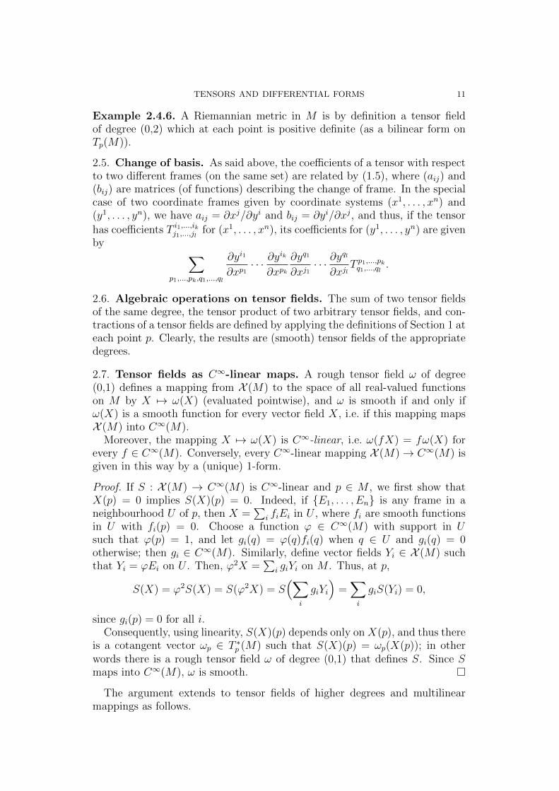
Example 2.4.6. A Riemannian metric in M is by definition a tensor fieldof degree (0,2) which at each point is positive definite (as a bilinear form onTp(M)).

2.5. Change of basis. As said above, the coefficients of a tensor with respectto two different frames (on the same set) are related by (1.5), where (aij) and(bij) are matrices (of functions) describing the change of frame. In the specialcase of two coordinate frames given by coordinate systems (x1, . . . , xn) and(y1, . . . , yn), we have aij = ∂xj/∂yi and bij = ∂yi/∂xj, and thus, if the tensor

has coefficients T i1,...,ikj1,...,jlfor (x1, . . . , xn), its coefficients for (y1, . . . , yn) are given

by ∑p1,...,pk,q1,...,ql

∂yi1

∂xp1· · · ∂y

ik

∂xpk∂yq1

∂xj1· · · ∂y

ql

∂xjlT p1,...,pkq1,...,ql

.

2.6. Algebraic operations on tensor fields. The sum of two tensor fieldsof the same degree, the tensor product of two arbitrary tensor fields, and con-tractions of a tensor fields are defined by applying the definitions of Section 1 ateach point p. Clearly, the results are (smooth) tensor fields of the appropriatedegrees.

2.7. Tensor fields as C∞-linear maps. A rough tensor field ω of degree(0,1) defines a mapping from X (M) to the space of all real-valued functionson M by X 7→ ω(X) (evaluated pointwise), and ω is smooth if and only ifω(X) is a smooth function for every vector field X, i.e. if this mapping mapsX (M) into C∞(M).

Moreover, the mapping X 7→ ω(X) is C∞-linear, i.e. ω(fX) = fω(X) forevery f ∈ C∞(M). Conversely, every C∞-linear mapping X (M)→ C∞(M) isgiven in this way by a (unique) 1-form.

Proof. If S : X (M) → C∞(M) is C∞-linear and p ∈ M , we first show thatX(p) = 0 implies S(X)(p) = 0. Indeed, if {E1, . . . , En} is any frame in aneighbourhood U of p, then X =

∑i fiEi in U , where fi are smooth functions

in U with fi(p) = 0. Choose a function ϕ ∈ C∞(M) with support in Usuch that ϕ(p) = 1, and let gi(q) = ϕ(q)fi(q) when q ∈ U and gi(q) = 0otherwise; then gi ∈ C∞(M). Similarly, define vector fields Yi ∈ X (M) suchthat Yi = ϕEi on U . Then, ϕ2X =

∑i giYi on M . Thus, at p,

S(X) = ϕ2S(X) = S(ϕ2X) = S(∑

i

giYi

)=∑i

giS(Yi) = 0,

since gi(p) = 0 for all i.Consequently, using linearity, S(X)(p) depends only on X(p), and thus there

is a cotangent vector ωp ∈ T ∗p (M) such that S(X)(p) = ωp(X(p)); in otherwords there is a rough tensor field ω of degree (0,1) that defines S. Since Smaps into C∞(M), ω is smooth. �

The argument extends to tensor fields of higher degrees and multilinearmappings as follows.

12 SVANTE JANSON

Theorem 2.7.1. Let T : X ∗(M)k × X (M)l → C∞(M) be a multilinear map-ping, where k, l ≥ 0. Then the following are equivalent:

(i) There exists a tensor field T of degree (k, l) such that (at every point)

T (ω1, . . . , ωk, X1, . . . , Xl) = T (ω1, . . . , ωk, X1, . . . , Xl).(ii) T is C∞-multilinear.

(iii) If ω1, . . . , ωk, ω′1, . . . , ω

′k, X1, . . . , Xl, X

′1, . . . , X

′l are 1-forms and vector

fields, respectively, such that ωi(p) = ω′i(p) and Xi(p) = X ′i(p) at somep ∈M , then T (ω1, . . . , ωk, X1, . . . , Xl)(p) = T (ω′1, . . . , ω

′k, X

′1, . . . , X

′l)(p).

(iv) If one of the fields ω1, . . . , ωk, X1, . . . , Xl vanishes at a point p, thenT (ω1, . . . , ωk, X1, . . . , Xl)(p) = 0.

Furthermore, if T is a tensor field of degree (1, l) for some l ≥ 0, then by

Example 1.2.5, it defines at each p ∈ M a multilinear map T : T ∗p (M)l →Tp(M) such that for any vector fields X1, . . . , Xl and a 1-form ω, we have atevery p

T (ω,X1, . . . , Xl) = 〈ω, T (X1, . . . , Xl)〉. (2.4)

It follows that, as p varies, T (X1, . . . , Xl) defines a vector field on M ; evidently

T is a C∞-multilinear mapping X (M)l → X (M). Conversely every such map-ping defines by (2.4) a C∞-multilinear mapping X ∗(M)× X (M)l → C∞(M),and thus by Theorem 2.7.1 a tensor field of degree (1, l). This yields thefollowing variant of Theorem 2.7.1.

Theorem 2.7.2. Let T : X (M)l → X (M) be a multilinear mapping, wherel ≥ 0. Then the following are equivalent.

(i) There exists a tensor field T of degree (1, l) such that (2.4) holds.(ii) T is C∞-multilinear.

(iii) If X1, . . . , Xl, X′1, . . . , X

′l are vector fields such that Xi(p) = X ′i(p) at

some p ∈M , then T (X1, . . . , Xl)(p) = T (X ′1, . . . , X′l)(p).

(iv) If one of the fields X1, . . . , Xl vanishes at a point p, then T (X1, . . . , Xl)(p)= 0.

Example 2.7.1. A Riemannian metric can equivalently be defined as a C∞-bilinear mapping g : X (M)2 → C∞(M) such that g(X,X) > 0 at every pointwhere X 6= 0.

Example 2.7.2. The Lie product (X, Y ) 7→ [X, Y ] of vector fields is a bilinearmapping X (M)2 → X (M), but it is not C∞-bilinear, and is thus not a tensor.

Example 2.7.3. An affine connection on M is a bilinear mapping X (M)2 →X (M) which it is not C∞-bilinear, and is thus not a tensor. This is also seenbecause its coefficients in a coordinate system (or for a general frame) do notobey the transformation rule (1.5).

Example 2.7.4. On the other hand, if ∇ is an affine connection and Y isa fixed vector field, then X 7→ ∇XY is a C∞-linear map X (M) → X (M),and can thus be regarded as a tensor field of degree (1,1). This tensor field isdenoted by ∇Y .


Example 2.7.5. If ∇ is an affine connection, then a simple calculation showsthat (X, Y ) 7→ ∇XY − ∇YX − [X, Y ] defines a C∞-bilinear map X (M)2 →X (M), and thus a tensor field of degree (1,2). This is called the torsiontensor (of the connection). The connection is called symmetic when its torsionvanishes, (The standard connection on a Riemannian manifold is symmetric,and thus there is no interest in the torsion tensor in Riemannian geometry.)

Example 2.7.6. If ∇ is an affine connection, then a somewhat longer calcu-lation shows that

(X, Y, Z) 7→ R(X, Y )Z := −∇X∇YZ +∇Y∇XZ +∇[X,Y ]Z

defines a C∞-trilinear map X (M)3 → X (M), and thus a tensor field of degree(1,3). This is the Riemann curvature tensor, generally denoted by R. (Manyauthors choose the opposite sign.)

We can contract the curvature tensor to a tensor of degree (0,2). This canbe done in three different ways, but for a Riemannian connection, one of themyields the zero tensor (by symmetry), and is thus not very interesting. (It isnon-zero for other affine connections, in general, but I do not know any useof this contraction.) The other two possibilities differ by sign only, again bysymmetry because R(X, Y )Z = −R(Y,X)Z from the definition, and one ofthem is called the Ricci tensor ; we define it by contraction of the contravariantand the second covariant index in R. (All authors make the choice dependingon their choice of sign for R, so that the sign of the Ricci tensor always isthe same; for example, the Ricci tensor for a sphere is a positive multiple ofthe metric tensor. However, do Carmo [2] uses a non-standard normalizationfactor 1/(n− 1) in his definition.)

2.8. Tensor bundles. The tensor bundle T k,l(M) of degree (k, l) is definedas the disjoint union of all tensor spaces T k,lp (M). Each coordinate system

(x1, . . . , xn) on an open set U defines a coordinate system on the correspondingpart T k,lp (U) =

⋃p∈U T

k,lp of T k,lp (M) by taking as coordinates of a tensor T ∈

T k,lp , p ∈ U , the n coordinates xi(p) followed by the nk+l coefficients of T for

the basis {∂/∂x1, . . . , ∂/∂xn}. It is easily seen that these coordinates systemsdefine a differentiable structure on T k,l(M), and thus the tensor bundle T k,l(M)is a differentiable manifold with dimension n+ nk+l.

Letting π : T k,l(M) → M denote the natural projection mapping a tensorT ∈ T k,lp to p, we can give an alternative (but equivalent) definition of a tensor

field of degree (k, l) as a differentiable function p 7→ T (p) of M into T k,l(M),such that π(T (p)) = p for every p. (Such functions are known as sections inthe bundle.

Example 2.8.1. T 0,0(M) = M × R.

Example 2.8.2. T 1,0(M) is the tangent bundle T (M).

Example 2.8.3. T 0,1(M) is called the cotangent bundle.

Remark. More generally, a vector bundle over a manifold M is a disjoint unionof a collection {Vp}p∈M of vector spaces of a fixed dimension N which is

14 SVANTE JANSON

equipped with a differentiable structure on the bundle that can be defined by acollection of open sets U covering M and for each of them a set of N functionse1, . . . eN from U into the bundle, such that, at each p ∈ U , e1(p), . . . eN(p)form a basis in Vp; a coordinate system for the bundle is defined by takingas coordinates of v ∈ Vp the coordinates of p in a coordinate system on M ,followed by the coordinates of v in the basis e1(p), . . . eN(p). (Hence, a vectorbundle is locally isomorphic to a product U ×RN , U ⊂M .) The vector spaceVp is called the fiber of the bundle at p. Sections of the bundle are defined asabove, thus yielding generalizations of vector fields and tensor fields.

Algebraic operations on vector spaces like taking the dual, direct sum, tensorproduct, . . . , yield (applied to the fibers) corresponding operations on vectorbundles, generalizing the constructions above.

For another example of a vector bundle, suppose that N is another manifoldand f : M → N a differentiable function, and define Vp = Tf(p)(N); this definesa vector bundle over M (known as the pull-back of the tangent bundle overN). If further f is an immersion, we can identify Tp(M) with the subspacedfp(Tp(M) of Tf(p)(N), and thus regard T (M) as a subbundle of the pull-back;if moreover N is a Riemannian manifold, we can define another bundle overM , the normal bundle of the immersion, as the subbundle of the pull-backwhose fiber Vp at p is the orthogonal complement of dfp(Tp(M) in Tf(p)(N),see [2, Section 6.3].

2.9. Covariant derivation of tensor fields. In any differentiable manifold,we can differentiate functions by a vector field (or by a tangent vector at asingle point). Given an affine connection, we can also differentiate vector fields(the covariant derivative). This extends to tensor fields of arbitrary degrees asfollows.

Let T k,l(M) denote the linear space of all tensor fields of degree (k, l) omM . (Thus T 0,0(M) = C∞(M) and T 1,0(M) = X (M).)

Theorem 2.9.1. If M is a differentiable manifold with an affine connection∇, there is a unique extension of ∇ to an operator (X,T ) 7→ ∇XT defined forany vector field X and tensor field T (of arbitrary degree) such that:

(i) For each k, l ≥ 0, ∇ is a bilinear mapping X (M) × T k,l(M) →T k,l(M). (Thus ∇XT has the same degree as T .)

(ii) ∇XT is further C∞-linear in X: ∇fXT = f∇XT for any f ∈ C∞(M)and tensor field T .

(iii) ∇X(fT ) = f∇XT + (Xf)T for any f ∈ C∞(M) and tensor field T .(iv) ∇Xf = Xf when f ∈ C∞(M), i.e. when f is a tensor field of degree

(0, 0).(v) ∇XY is the vector field given by the connection when Y is a vector

field, i.e. when Y is a tensor field of degree (1, 0).(vi) ∇X(T ⊗U) = (∇XT )⊗U +T ⊗∇XU for any two tensor fields T and

U .(vii) ∇X commutes with contractions.


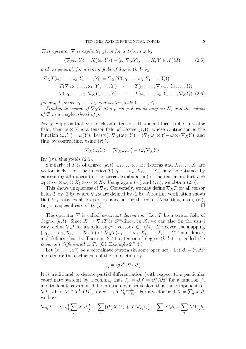
This operator ∇ is explicitly given for a 1-form ω by

〈∇Xω, Y 〉 = X(〈ω, Y 〉)− 〈ω,∇XY 〉, X, Y ∈ X (M), (2.5)

and, in general, for a tensor field of degree (k, l) by

∇XT (ω1, . . . , ωk, Y1, . . . , Yl) = ∇X

(T (ω1, . . . , ωk, Y1, . . . , Yl)

)− T (∇Xω1, . . . , ωk, Y1, . . . , Yl)− · · · − T (ω1, . . . ,∇Xωk, Y1, . . . , Yl)

− T (ω1, . . . , ωk,∇XY1, . . . , Yl)− · · · − T (ω1, . . . , ωk, Y1, . . . ,∇XYl) (2.6)

for any 1-forms ω1, . . . , ωk and vector fields Y1, . . . , Yl.Finally, the value of ∇XT at a point p depends only on Xp and the values

of T in a neigbourhood of p.

Proof. Suppose that ∇ is such an extension. If ω is a 1-form and Y a vectorfield, then ω ⊗ Y is a tensor field of degree (1,1), whose contraction is thefunction 〈ω, Y 〉 = ω(Y ). By (vi), ∇X(ω⊗Y ) = (∇Y ω)⊗Y +ω⊗ (∇XY ), andthus by contracting, using (vii),

∇X〈ω, Y 〉 = 〈∇Xω, Y 〉+ 〈ω,∇XY 〉.

By (iv), this yields (2.5).Similarly, if T is of degree (k, l), ω1, . . . , ωk are 1-forms and X1, . . . , Xl are

vector fields, then the function T (ω1, . . . , ωk, X1, . . . , Xl) may be obtained bycontracting all indices (in the correct combination) of the tensor product T ⊗ω1 ⊗ · · · ⊗ ωk ⊗X1 ⊗ · · · ⊗Xl. Using again (vi) and (vii), we obtain (2.6).

This shows uniqueness of ∇X . Conversely, we may define ∇XT for all tensorfields T by (2.6), where ∇Xω are defined by (2.5). A routine verification showsthat ∇X satisfies all properties listed in the theorem. (Note that, using (iv),(iii) is a special case of (vi).) �

The operator ∇ is called covariant derivation. Let T be a tensor field ofdegree (k, l). Since X 7→ ∇XT is C∞-linear in X, we can also (in the usualway) define ∇vT for a single tangent vector v ∈ T (M). Moreover, the mapping(ω1, . . . , ωk, X1, . . . , Xl, X) 7→ ∇XT (ω1, . . . , ωk, X1, . . . , Xl) is C∞-multilinear,and defines thus by Theorem 2.7.1 a tensor of degree (k, l + 1), called thecovariant differential of T . (Cf. Example 2.7.4.)

Let (x1, . . . , xn) be a coordinate system (in some open set). Let ∂i = ∂/∂xi

and denote the coefficients of the connection by

Γkij = 〈dxk,∇∂j∂i〉.

It is traditional to denote partial differentiation (with respect to a particularcoordinate system) by a comma, thus f,i = ∂if = ∂f/∂xi for a function f ,and to denote covariant differentiation by a semicolon, thus the components of∇T , where T ∈ T k,l(M), are written T i1,...,ikj1,...,jl;j

. For a vector field X =∑

iXi∂i

we have

∇∂jX = ∇∂j

(∑i

X i∂i

)=∑i

((∂jX

i)∂i +X i∇∂j∂i)

=∑i

X i,j∂i +

∑ik

X iΓkij∂j

16 SVANTE JANSON

and thusX i

;j = X i,j +

∑m

XmΓimj.

It now follows from (2.5) that for a 1-form ω,

ωi;j = 〈∇∂jω, ∂i〉 = ωi,j −∑k

ωkΓkij.

In particular, ∇∂jdxk = −

∑i Γ

kijdx

i and

∇dxk = −∑ij

Γkijdxi ⊗ dxj.

In general, (2.6) now implies that for a tensor T of degree (k, l),

T i1,...,ikj1,...,jl;j= T i1,...,ikj1,...,jl,j

+∑m

Tm,i2,...,ikj1,...,jlΓi1mj + · · ·+

∑m

Ti1,...,ik−1,mj1,...,jl

Γikmj

−∑m

T i1,...,ikm,j2,...,jlΓmj1j − · · · −

∑m

T i1,...,ikj1,...,jl−1,mΓmjlj.

Remark. Given a vector bundle, an operator ∇ that for each vector field Xand section S of the bundle yields a section ∇XS satisfying the analogues ofconditions (i)–(iii) in Theorem 2.9.1 is called an affine connection in the bundle.An affine connection on a manifold is thus the same as an affine connection inthe tangent bundle, and the theorem says that it defines a natural connectionin each tensor bundle.

Now consider a Riemannian manifold with a metric tensor g and an arbitraryaffine connection ∇. If X and Y are two vector fields, we have by (2.6), forany vector fields X, Y, Z,

∇g(Y, Z,X) = (∇Xg)(Y, Z) = X(g(Y, Z))− g(∇XY, Z)− g(Y,∇XZ). (2.7)

The condition on the Riemannian (Levi-Civita) connection that X(g(Y, Z)) =g(∇XY, Z) + g(Y,∇XZ) can thus be written as ∇g = 0. In other words, theRiemannian connection is characterized as the unique affine connection thatis symmetric (cf. Example 2.7.5) and is such that ∇g = 0.

2.10. Tensors on a Riemannian manifold. Suppose that M is a Riemann-ian manifold, with metric tensor g and Riemannian (Levi-Civita) connection∇. Recall from Section 2.9 that ∇g = 0.

We can raise or lower indices of tensors on M using the Riemannian metricg, by applying the isomorphisms described in Section 1.9 at each point p; recallthat the Riemannian metric by definition makes each Tp(M) into a Euclideanspace. Thus there

Example 2.10.1. The curvature tensor R has a covariant form (also denotedby R), which is a covariant tensor of degree 4. The connection with the tensorof degree (1, 3) defined in Example 2.7.6 is

R(X, Y, Z,W ) = 〈R(X, Y )Z,W 〉,for arbitrary vector fields (or just tangent vectors at a single point) X, Y, Z,W .


Example 2.10.2. For the coefficients in a coordinate system let, as usual, gij

be the coefficients of the dual inner product so that (gij) is the matrix inverseof (gij). If Rl

ijk and Rijkl denote two forms of the Riemann curvature tensor,Rij the Ricci tensor and R the scalar curvature obtained by contracting theRicci tensor, we have

Rlijk =

∑m

glmRijkm

Rijkl =∑m

glmRmijk

Rij =∑k

Rkikj =

∑k,l

gklRikjl =∑k,l

gklRkilj

R =∑i,j

gijRij =∑i,j,k,l

gikgjlRijkl.

If X is a vector field and T is any tensor field, then ∇X(g ⊗ T ) = (∇Xg)⊗T + g ⊗ ∇XT = g ⊗ ∇XT by Theorem 2.9.1(vi). Since lowering an index ofT can be described as taking the tensor product with g followed by a contrac-tion (Section 1.9), and ∇X commutes with contractions, it follows that ∇X

commutes with lowerings of indices, and thus also with raisings of indices.

Example 2.10.3. The covariant form of the Riemann curvature tensor hascoefficients Rijkl in a coordinate system, and its covariant differential ∇R hascoefficients Rijkl;m. The Bianchi identities are

Rijkl +Riklj +Riljk = 0

and

Rijkl;m +Rijlm;k +Rijmk;l = 0.

Raising the indices i and j in the second Bianchi identity and contracting thetwo pairs (i, k) and (j, l), we obtain, since covariant differentiation commuteswith contractions and raisings of indices,

R;m −∑i

Rim;i −

∑l

Rlm;l = 0,

where Rij denotes the coefficients of (the mixed form of) the Ricci tensor,

and R =∑

iRii is the scalar curvature. It follows that if Ei

j = Rij − 1

2δijR

denotes the coefficients of the mixed form of the Einstein tensor, then, usingthe easily verified fact that the tensor ι with coefficients δij has ∇ι = 0 (cf.Example 1.9.2), ∑

i

Eij;i = 0.

(The covariant form of the Einstein tensor is Eij = Rij − 12Rgij.)

18 SVANTE JANSON

3. Differential forms

A differential form of degree k, often simply called a k-form, on a manifoldis an antisymmetric covariant tensor field (of degree k). More generally, wecan define a differential form as a (formal) sum ω0 +ω1 + · · ·+ωn, where ωk isa differential form of degree k. The value at a point p of a differential form isthus an element of the exterior algebra A(Tp(M)); if the differential form hasdegree k, then the value belongs to the subspace Ak(Tp(M)).

By Theorem 2.7.1, a k-form may be regarded as an antisymmetric C∞-multilinear mapping ω : X (M)k → C∞(M).

We let Ek(M) denote the linear space of all k-forms on M , and E∗(M) =⊕nk=0E

k(M) the linear space of all differential forms.

Remark. Using the theory of vector bundles, we may form the exterior bundleA(M) =

⋃p∈M A(Tp(M)) and its subbundles Ak(M) =

⋃p∈M Ak(Tp(M)), 0 ≤

k ≤ n. A differential form (of degree k) is then a section in the exterior bundle(in Ak(M)).

We form the sum and exterior product of two differential forms by perform-ing the operations pointwise; thus the space E∗(M) of all differential formsbecomes an algebra. This algebra is associative but not commutative; it is by(1.7) anticommutative in the sense that

ω2 ∧ ω1 = (−1)klω1 ∧ ω2, ω1 ∈ Ek(M), ω2 ∈ El(M). (3.1)

3.1. Bases. Given a frame {E1, . . . , En} in an open subset U of M , the dualframe {E1, . . . , En} gives a basis in T ∗q (M) for every q ∈ U , and by takingexterior products, we obtain a basis in each Ak(Tp(M)).

In particular, if (x1, . . . , xn) is a coordinate system in an open set U , thedifferentials dx1, . . . , dxn form a basis in each T ∗q (M), and the exterior products

dxi1 ∧ . . . dxik , i1 < · · · < ik, form a collection of differential forms on U thatyield a basis in Ak(Tq(M)) for every q ∈M (0 ≤ k ≤ n). Hence, any differentialform on U may uniquely be written

n∑k=0

∑1≤i1<...ik≤n

ai1,...,ikdxi1 ∧ · · · ∧ dxik , (3.2)

for some smooth functions ai1,...,ik on U .

3.2. Exterior differentiation. If f is a smooth function on M , i.e. a 0-form,its differential df was defined in Section 2 as a cotangent field, i.e. a 1-form(Section 2.1 and Example 2.4.5). This operation d has an important extensionto differential forms described by the following theorem; d is called exteriordifferentiation.

Theorem 3.2.1. There exists a unique operator d : E∗(M) → E∗(M) withthe following properties:

(i) d : E∗(M)→ E∗(M) is linear.(ii) If ω ∈ Ek(M), then dω ∈ Ek+1(M).


(iii) If ω1 ∈ Ek(M) and ω2 ∈ El(M), then

d(ω1 ∧ ω2) = (dω1) ∧ ω2 + (−1)kω1 ∧ (dω2).

(iv) d ◦ d = 0, i.e. d(dω) = 0 for every ω ∈ E∗(M).(v) If f ∈ E0(M) = C∞(M), then df ∈ E1(M) is the differential of f

given by df(X) = Xf , X ∈ X (M).

Moreover, d is a local operator in the sense that for every p ∈ M , dω(p)depends only on the values of ω in a neighbourhood of p (i.e. on the germ of ωat p). Explicitly, in a coordinate system, d is given by

d(∑

ai1,...,ikdxi1 ∧ · · · ∧ dxik

)=∑

dai1,...,ikdxi1 ∧ · · · ∧ dxik

=∑ ∂ai1,...,ik

∂xjdxj ∧ dxi1 ∧ · · · ∧ dxik . (3.3)

Proof. Suppose first that M is covered by a single coordinate neighbourhood,and let (x1, . . . , xn) be a global coordinate system. Then every differential formon M can be written as (3.2) for some smooth functions ai1,...,ik . If d satifiesthe conditions, then (3.3) follows directly, which further shows that d is localand unique. Conversely, we may define d by (3.3), and it is easily verified that(i)–(v) hold. (For (iv), first note that if f is a smooth function, then

ddf = d(∑

i

∂f

∂xidxi)

=∑i,j

∂2f

∂xi∂xjdxj ∧ dxi = 0,

because ∂2f∂xi∂xj

= ∂2f∂xj∂xi

and dxj ∧ dxi = −dxi ∧ dxj. The general case thenfollows by (3.3).)

For a general manifold M , suppose that d satisfies (i)–(v). First, assumethat p ∈M and that ω1, ω2 ∈ E∗(M) coincide in a neighbourhood V of p. Letω = ω1 − ω2 and choose ϕ ∈ C∞(M) such that ϕ(p) = 1 and suppϕ ⊂ V .Then ϕω = 0 and dϕ∧ω = 0, and since (iii) yields d(ϕω) = dϕ∧ω+ϕ∧dω, weobtain ϕdω = ϕ ∧ dω = 0. In particular dω(p) = 0 and thus dω1(p) = dω2(p).This shows that d is a local operator.

Next, let U be an open subset of M . If ω ∈ E∗(U) and p ∈ U , we canfind ω ∈ E∗(M) such that ω = ω in a neighbourhood of p. By the fact justshown that d is local, dω(p) does not depend on the choice of ω, so we mayuniquely define dUω(p) = dω(p). It is easily seen that dUω ∈ E∗(U) and thatwe have defined an operator dU : E∗(U) → E∗(U) that satisfies (i)–(v) on U .In particular, if U is a coordinate neighbourhood, the first part of the proofapplies and shows that dU is given by (3.3). Moreover, if ω ∈ E∗(M) and ωU isthe restriction of ω to U , we can choose ωU = ω which shows that dω = dUωUon U . Consequently, dω is given by (3.3) on U . This further shows uniquenessin the general case.

For existence, finally, we can for any ω ∈ E∗(M) use (3.3) to define dω in anycoordinate neighbourhood. We must, however, verify that these definitions areconsistent. Thus, suppose that U and U are two open sets where coordinatesystems (x1, . . . , xn) and (x1, . . . , xn), respectively, are defined, and define thecorresponding operators dU on E∗(U) and dU on E∗(U) by (3.3), using the

20 SVANTE JANSON

respective coordinate systems. On the intersection U ∩ U , both coordinatesystems are defined and thus define differentiation operators in E∗(U ∩ U) by(3.3); by the uniqueness shown in the first part of the proof, these operatorscoincide, and thus dUω = dUω on U ∩ U for any ω ∈ E∗(M), which is therequied consistency. Hence, dω is well defined, and it is easily checked that(i)–(v) hold. �

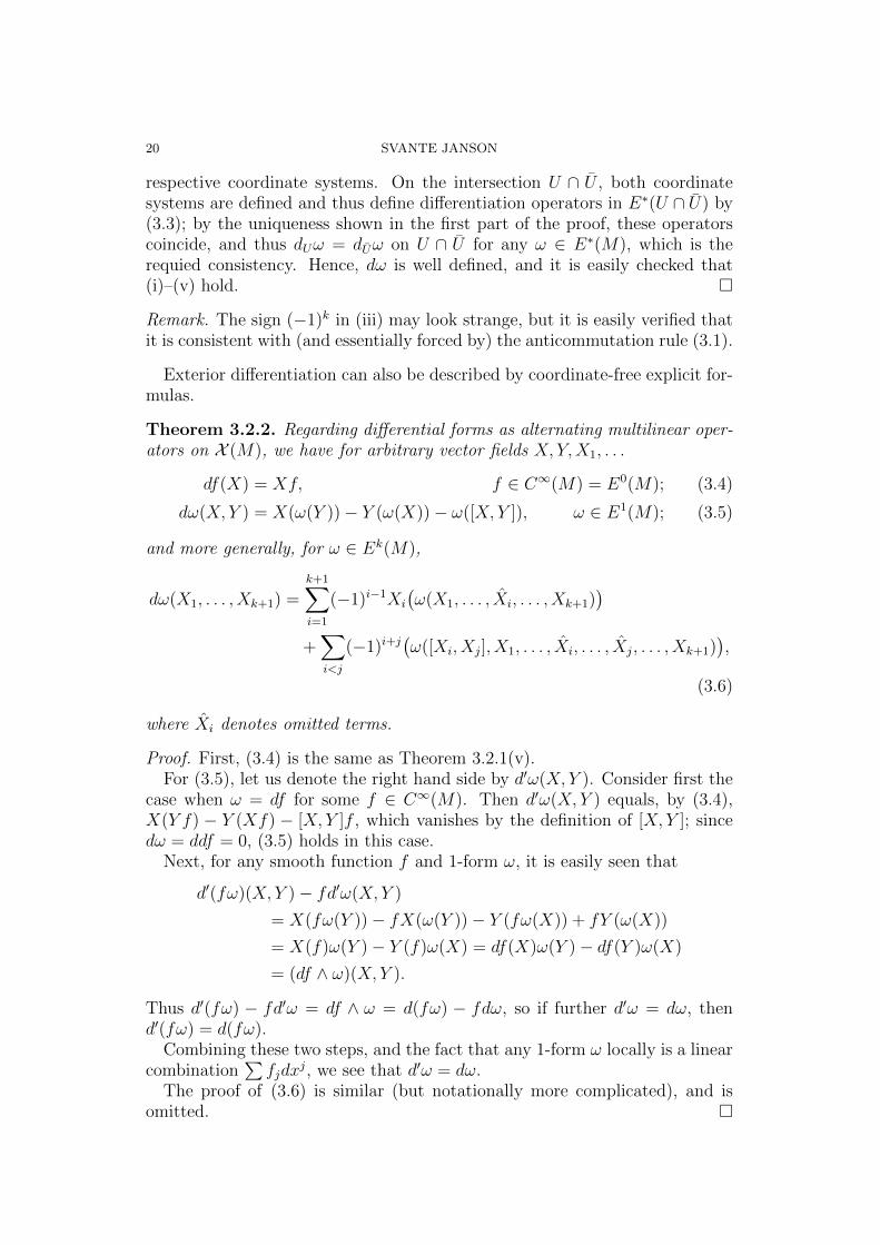
Remark. The sign (−1)k in (iii) may look strange, but it is easily verified thatit is consistent with (and essentially forced by) the anticommutation rule (3.1).

Exterior differentiation can also be described by coordinate-free explicit for-mulas.

Theorem 3.2.2. Regarding differential forms as alternating multilinear oper-ators on X (M), we have for arbitrary vector fields X, Y,X1, . . .

df(X) = Xf, f ∈ C∞(M) = E0(M); (3.4)

dω(X, Y ) = X(ω(Y ))− Y (ω(X))− ω([X, Y ]), ω ∈ E1(M); (3.5)

and more generally, for ω ∈ Ek(M),

dω(X1, . . . , Xk+1) =k+1∑i=1

(−1)i−1Xi

(ω(X1, . . . , Xi, . . . , Xk+1)

)+∑i<j

(−1)i+j(ω([Xi, Xj], X1, . . . , Xi, . . . , Xj, . . . , Xk+1)

),

(3.6)

where Xi denotes omitted terms.

Proof. First, (3.4) is the same as Theorem 3.2.1(v).For (3.5), let us denote the right hand side by d′ω(X, Y ). Consider first the

case when ω = df for some f ∈ C∞(M). Then d′ω(X, Y ) equals, by (3.4),X(Y f) − Y (Xf) − [X, Y ]f , which vanishes by the definition of [X, Y ]; sincedω = ddf = 0, (3.5) holds in this case.

Next, for any smooth function f and 1-form ω, it is easily seen that

d′(fω)(X, Y )− fd′ω(X, Y )

= X(fω(Y ))− fX(ω(Y ))− Y (fω(X)) + fY (ω(X))

= X(f)ω(Y )− Y (f)ω(X) = df(X)ω(Y )− df(Y )ω(X)

= (df ∧ ω)(X, Y ).

Thus d′(fω) − fd′ω = df ∧ ω = d(fω) − fdω, so if further d′ω = dω, thend′(fω) = d(fω).

Combining these two steps, and the fact that any 1-form ω locally is a linearcombination

∑fjdx

j, we see that d′ω = dω.The proof of (3.6) is similar (but notationally more complicated), and is

omitted. �


3.3. Closed and exact forms. A differential form ω is closed if dω = 0, andexact if ω = dω for some differential form ω, i.e. if ω ∈ Im(d).

Since d ◦ d = 0, every exact form is closed. For k-forms with k ≥ 1, theconverse is true locally, for example in any open set diffeomorphic to an openball in Rn (the Poincare lemma, see [1, 3] for proofs), but not always globally.(The case of 0-forms is trivial: there are no exact 0-forms except 0, while everyconstant function is a closed 0-form; in a connected manifold the constants arefurthermore the only closed 0-forms.)

Example 3.3.1. Let M = R2 \ {0}. Then ω = (x dy − y dx)/(x2 + y2) is aclosed 1-form that is not exact. This can be verified by direct computations,but it is more illuminating to observe that in any subset of M where we candefine a continuous branch of arg(x+ iy) = Im log(x+ iy), we have ω = d arg.This shows that ω is closed (locally and thus globally); it also shows that ifω = df for some function f , then f would have to be a constant plus a globallydefined continuous branch of arg, which is impossible.

The de Rham cohomology groups are defined as the quotient spaces

Hk(M) = {closed k-forms}/{exact k-forms}.

Thus Hk(M) = 0 if and only if every closed k-form is exact.It turns out that the cohomology groups are finite-dimensional in many

cases, for example whenever M is compact. In a vague sense, the dimension ofHk(M) (known as the Betti number) is the number of k-dimensional “holes”in M .

Remark. For any manifold M , the de Rham cohomology groups are isomorphicto the singular and Cech cohomology groups (with real coefficients) defined inalgebraic topology, see [3].

Example 3.3.2. Hk(Rn) = 0 for every k ≥ 1.Hk(Sn) = 0 for 1 ≤ k < n (and trivially for k > n), while Hn(Sn) ∼= R.

3.4. Classical vector analysis. Classically, a vector field on R3 (or on anopen subset) is a (smooth) function into R3, or equivalently a triple (f1, f2, f3)of smooth real-valued functions. This can be identified with the vector field(in general differential geometry sense) f1∂/∂x

1 + f2∂/∂x2 + f3∂/∂x

3.We can also identify a 1-form f1 dx

1 + f2 dx2 + f3 dx

3 with the vector field(f1, f2, f3); this amounts to identifying a 1-form and the vector field obtainedby raising the index as in Sections 1.9 and 2.10.

Moreover, a 2-form may be written f12 dx1 ∧ dx2 + f13 dx

1 ∧ dx3 + f23 dx2 ∧

dx3, and we may identify this with the vector field (f23,−f13, f12); the orderand signs of the functions are chosen such that if ω is a 2-form and F thecorresponding vector field, and λ is any 1-form, then

λ ∧ ω = 〈λ, F 〉dx1 ∧ dx2 ∧ dx3. (3.7)

Finally, a 3-form can be written f dx1 ∧ dx2 ∧ dx3 and identified with thefunction f .

22 SVANTE JANSON

With these identifications, the exterior differentiation d yields three classicaloperators: d : E0(R3) → E1(R3) becomes the gradient grad : C∞ → X ,d : E1(R3) → E2(R3) becomes the curl : X → X , and d : E2(R3) → E3(R3)becomes the divergence div : X → C∞.

The fact that d ◦ d = 0 thus says that the gradient of a function is curl-free,and that the curl of a vector field is divergence-free. Conversely, the Poincarelemma says that (globally or in a suitable, for example convex, subset), everycurl-free vector field is the gradient of some function, and that every divergence-free vector field is the curl of another vector field.

3.5. Gradient and divergence on Riemannian manifolds. While the curlstudied in Section 3.4 is a special phenomenon in three dimensions, the gradientand divergence may be defined in any Riemannian manifold M . First, if f ∈C∞(M), then df is a 1-form, and we define grad f as the corresponding vectorfield, obtained by raising the index.

Secondly, if X is a vector field, its covariant derivative ∇X is a tensorof degree (1,1), and we define divX to be the contraction of ∇X. Thusgrad : C∞(M)→ X (M) and div : X (M)→ C∞(M).

The composition div grad : C∞(M) → C∞(M) is known as the Laplace-Beltrami operator ∆. Equivalently, ∆f is the contraction of the second covari-ant derivative ∇∇f ∈ T 0,2(M), and in a coordinate system we have

∆f =∑i,j

gijf;ij.

Remark. The divergence can also be described using an isomorphism betweenvector fields and (n − 1)-forms as in the case of R3 studied above. Moregenerally, if M is oriented (otherwise we can work locally), there exists aunique n-form ω0 such that if (x1, . . . , xn) is any oriented coordinate system,then

ω0 = (det(gij)ij)1/2dx1 ∧ · · · ∧ dxn. (3.8)

There are now isomorphisms C∞(M) ∼= En(M) and X (M) ∼= En−1(M) suchthat a function f corresponds to the n-form fω0, and a vector field X to theunique (n− 1)-form ω such that λ ∧ ω = 〈λ,X〉ω0 for every 1-form λ. It maythen be verified that d : En−1(M) → En(M) corresponds to div : X (M) →C∞(M).

3.6. Pull-backs. Suppose that ϕ : M → N is a smooth mapping between twomanifolds. If f : N → R is a smooth function on N , then f ◦ ϕ is a smoothfunction on M . This operation extends in a natural way to differential forms.

Theorem 3.6.1. There is a unique linear map ϕ∗ : E∗(N)→ E∗(M) such thatϕ∗(f) = f ◦ϕ for f ∈ C∞(M) = E0(N), ϕ∗(dω) = d(ϕX(ω)) and ϕ∗(ω1∧ω2) =(ϕ∗ω1) ∧ (ϕ∗ω2) for arbitrary differential forms ω, ω1, ω2.

The operator ϕ∗ is known as the pull-back.


4. Integration of differential forms

Consider an n-form ω on the n-dimensional manifold M . If x = (x1, . . . , xn)is a coordinate system in an open set U , then ω = f dx1 ∧ · · · ∧ dxn in U forsome smooth function f .

If y = (y1, . . . , yn) is another coordinate system, defined in an open set U ′,say, then we also have ω = g dy1 ∧ · · · ∧ dyn in U ′. On the intersection U ∩U ′,dyi =

∑j∂yi

∂xjdxj and thus, by (1.9),

dy1 ∧ · · · ∧ dyn = J dx1 ∧ · · · ∧ dxn,where J = det

((∂yi/∂xj)ni,j=1

)is the Jacobian of the change of coordinates

y ◦ x−1. Consequently, ω = g dy1 ∧ · · · ∧ dyn = gJ dx1 ∧ · · · ∧ dxn, and thusf = gJ .

We here regard f , g and J as functions defined on (subsets of) M ; thecoordinate representations are the functions f = f ◦ x−1 defined on x(U),g = g ◦ y−1 defined on y(U ′), and J = J ◦ x−1 defined on x(U ∩ U ′) (all threeare open subsets of Rn).

Next, let K be a compact (for convenience) subset of U∩U ′. By the standardformula for a change of variables in a multidimensional integral,∫

y(K)

g dy1 · · · dyn =

∫x(K)

g ◦ (y ◦ x−1)|J | dx1 · · · dxn

=

∫x(K)

g ◦ x−1|J ◦ x−1| dx1 · · · dxn

=

∫x(K)

f ◦ x−1 sgn(J ◦ x−1) dx1 · · · dxn

=

∫x(K)

f sgn(J) dx1 · · · dxn.

Consequently, if the two coordinate systems x and y have the same orientation,i.e. J > 0, then

∫y(K)

g =∫x(K)

f , while the two integrals differ by sign if the

two coordinate systems have different orientations.From now on, suppose that M is an oriented manifold. The argument just

given shows that if ω is an n-form and K is a compact subset of M that iscovered by a single coordinate neighbourhood, then we may uniquely define∫

K

ω =

∫x(K)

f dx1 · · · dxn

for any positively oriented coordinate system x = {e1, . . . , en} defined on K,with f as above. A routine argument using partitions of K or of ω then showsthat we may (in a natural way, preserving linearity properties) define

∫Kω

for any n-form ω and any compact subset K of M , and∫Mω for any n-form

ω with compact support. The compactness conditions may be relaxed to anintegrability condition.

Remark. Note that only n-forms can be integrated over an n-dimensional man-ifold. However, forms of lower degree can be integrated over submanifolds of

24 SVANTE JANSON

the corresponding dimension. Thus, if ω is a k-form and N is a k-dimensionalsubmanifold of M , then the restriction (i.e. the pull-back) of ω to N is a k-formon N and

∫Nω is defined provided, for example, ω has compact support in N .

Similarly, if α : (a, b) → M is a (smooth) curve and ω is a 1-form, theintegral

∫αω is defined (under suitable integrability restrictions) by integrating

the pull-back of ω to (a, b); it is easily verified that this integral is independentof the parametrization of α. Thus line integrals of 1-forms are defined verygenerally.

4.1. Integration on Riemannian manifolds. Every Riemannian manifold(oriented or not) carries a natural measure, which in a coordinate system(x1, . . . , xn) is given by

dµ =√

det((gij)ij) dx1 · · · dxn. (4.1)

(This equals the n-dimensional Hausdorff measure defined by the metric.)Thus we may integrate functions on a Riemannian manifold. If M is ori-

ented, and ω0 is the special n-form defined (3.8), then∫Mf =

∫Mfω0, so the

two notions of integration correspond in a natural way.

4.2. Stokes’ theorem. Let M be an oriented manifold. A regular domainin M is a subset of the form {p ∈ M : f(p) > 0} for some smooth functionf : M → R such that df 6= 0 at every point p with f(p) = 0; equivalently(as follows by a partition of unity argument), D is an open subset such thatevery boundary point p ∈ ∂U has a neighbourhood U with a smooth functionf : U → R such that df 6= 0 in U and D ∩ U = {p ∈ U : f(p) > 0}.

If D is a regular domain, then its boundary ∂D is an (n − 1)-dimensionalmanifold, embedded in M . The orientation of M induces an orientation of ∂D;we choose the orientation such that if p ∈ ∂D and v ∈ Tp(M) \ Tp(∂D) is anouter tangent vector, meaning that v = α′(0) for some curve α with α(0) = pand α(t) /∈ M for t > 0, then v1, . . . , vn−1 is an oriented basis in Tp(∂D) ifand only if v, v1, . . . , vn−1 is an oriented basis in Tp(M). Then Stoke’s theoremmay be stated as follows.

Theorem 4.2.1 (Stokes). Let D be a regular domain in an oriented manifoldM of dimension n, and let ∂D have the induced orientation. If ω is an (n−1)-form on M , and either D or suppω is compact, then∫

D

dω =

∫∂D

ω.

Proof. Using a partition of unity and suitable coordinate mappings, the theo-rem is reduced to the case where D is the upper half space in M = Rn and ωhas compact support, which is verified by a simple calculation. �

Corollary 4.2.1. If M is an oriented n-dimensional manifold and ω is an(n− 1)-form on M with compact support, then∫

M

dω = 0.


Remark. An essentially equivalent, but sometimes more elegant version ofStokes’ theorem uses the notion of manifolds with boundary instead of reg-ular domains, see [1].

This general version of Stokes’ theorem contains several standard resultsfrom calculus.

Example 4.2.1. If D is a bounded regular domain in R2 and ω = f dx+ g dyis a 1-form, then Stokes’ theorem yields∫

D

(∂g

∂x− ∂f

∂y

)dx ∧ dy =

∫∂D

f dx+ g dy,

where the left hand side is an ordinary Riemann integral (we may replacedx ∧ dy by dx dy) and the right hand side is a line integral. This is known asGreen’s theorem.

Example 4.2.2. Let M be a smooth surface in R3, and D a regular domainin M , i.e. a portion of the surface bounded by smooth curves. Denote the unitnormal to M (suitably oriented) by n. Let ω = f dx+g dy+h dz be a 1-form inR3, and let F = (f, g, h) denote the corresponding vector field as in Section 3.4.If ω0 is the special 2-form on M defined by (3.8) and ω0 = dx ∧ dy ∧ dz isthe corresponding special 3-form on R3, then ω0 = n ∧ ω0 on M . Thus, ifdω = ϕω0, we have n ∧ dω = ϕω0. On the other hand, by Section 3.4, inparticular (3.7), n ∧ dω = 〈n, curlF 〉ω0; hence ϕ = 〈n, curlF 〉. Consequently,Stokes’ theorem yields∫

∂D

f dx+ g dy + h dz =

∫D

dω =

∫D

〈n, curlF 〉,

where the final integral is an ordinary integral with respect to surface measure,cf. Section 4.1.

Example 4.2.3. In a Riemannian manifold, for example in Rn, the isomor-phisms in the remark in Section 3.5 yield the following version of Stokes’ the-orem, known as the divergence theorem.

Theorem 4.2.2. Let D be a regular domain in a Riemannian manifold M ,and let, for p ∈ ∂D, n(p) be the outer unit normal to D. If X is a vector fieldon M , and either D or suppX is compact, then∫

D

divX =

∫∂D

〈X,n〉.

Here both integrals are ordinary (Lebesgue) integrals with respect to thestandard measure (4.1) in a Riemannian manifold.

References

[1] W. Boothby, An Introduction to Differentiable Manifolds and Riemannian Geometry.Academic Press, New York, 1975.

[2] M. do Carmo, Riemannian Geometry. Birkhauser, Boston, 1992.[3] F. Warner, Foundations of Differentiable Manifolds and Lie Groups. Springer, New

York, 1983.

26 SVANTE JANSON

Department of Mathematics, Uppsala University, PO Box 480, S-751 06 Upp-sala, Sweden

E-mail address: [email protected]

Documents

Introduction Tensors over a vector space Remark. The …svante/papers/sjN2.pdf · · 2011-04-17Introduction The purpose of these ... Tensors over a vector space ... There is also