Embed Size (px)
Citation preview
Introduction to MATLABDr./ Ahmed Nagib
Mechanical Engineering department, Alexandria university, Egypt
Sep 2015
Chapter 3
Numeric, Cell, and Structure Arrays
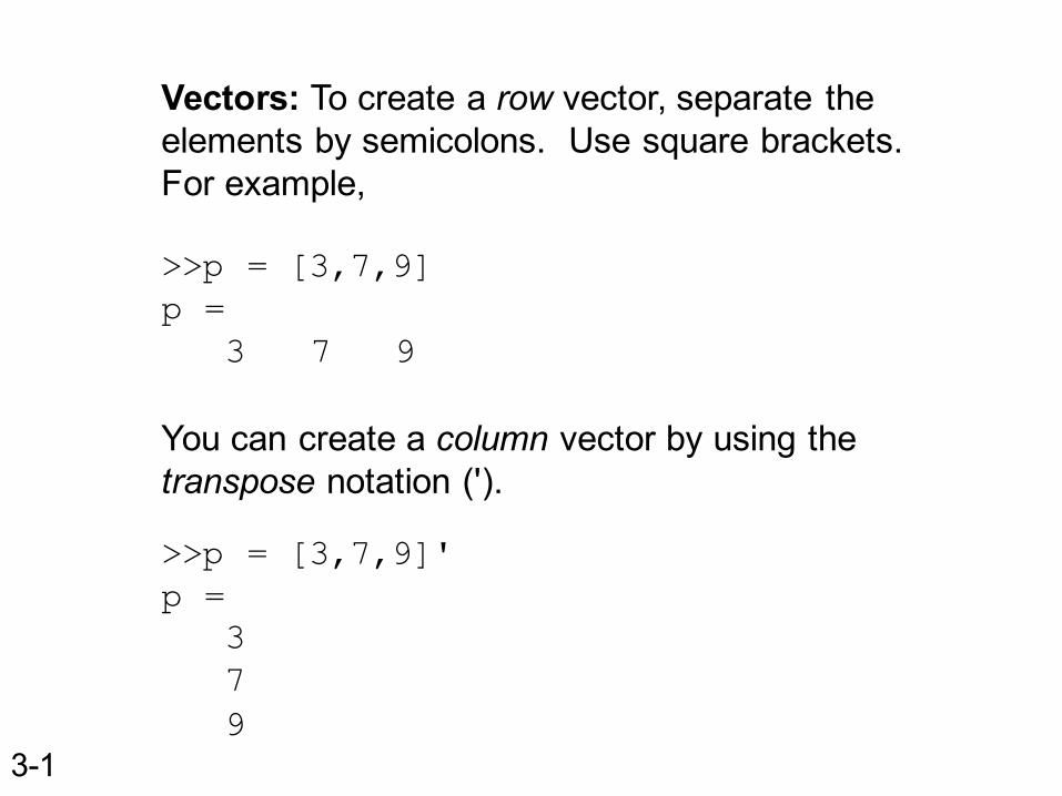
Vectors: To create a row vector, separate the elements by semicolons. Use square brackets. For example,
>>p = [3,7,9]p =
3 7 9
You can create a column vector by using the transpose notation (').
>>p = [3,7,9]'p =
379
3-1
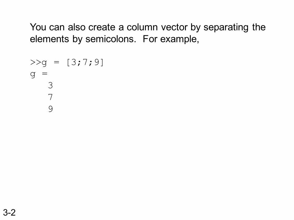
You can also create a column vector by separating the elements by semicolons. For example,
>>g = [3;7;9]g =
379
3-2
3-3
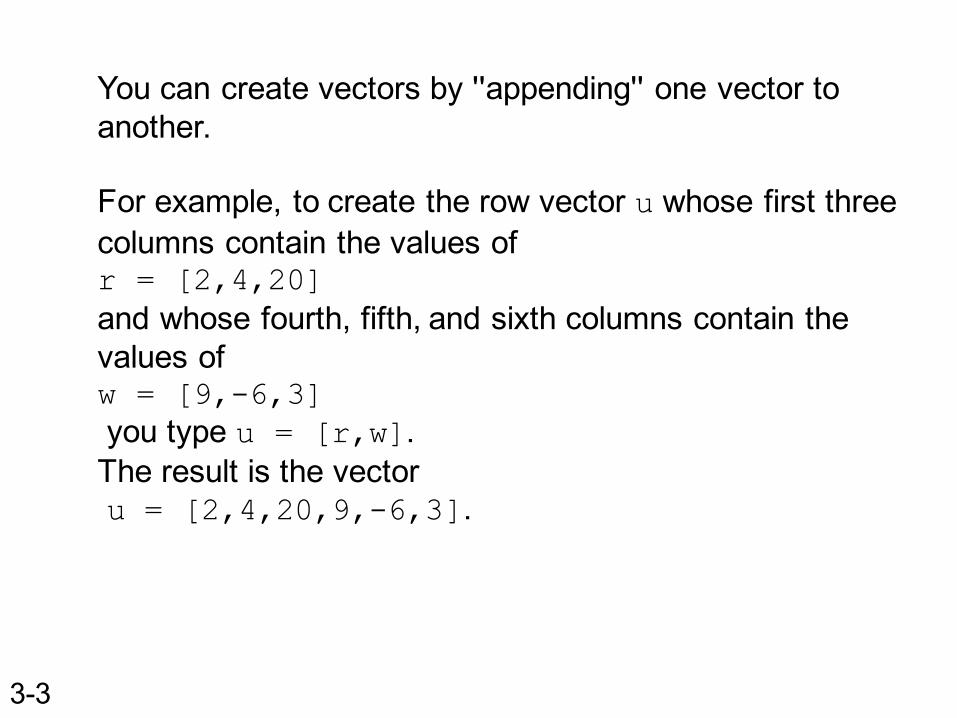
You can create vectors by ''appending'' one vector to another.
For example, to create the row vector u whose first three columns contain the values of r = [2,4,20]and whose fourth, fifth, and sixth columns contain the values of w = [9,-6,3]you type u = [r,w]. The result is the vectoru = [2,4,20,9,-6,3].
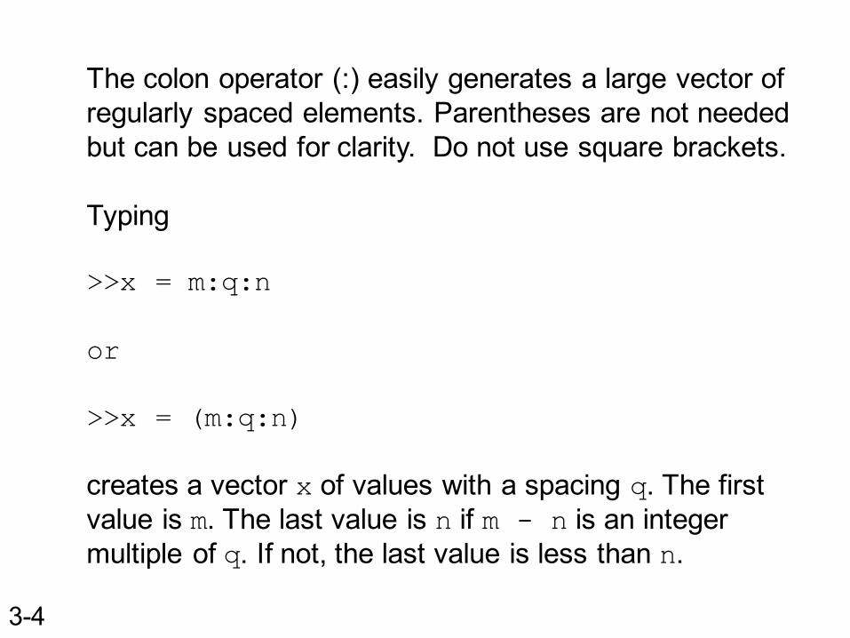
The colon operator (:) easily generates a large vector of regularly spaced elements. Parentheses are not needed but can be used for clarity. Do not use square brackets.
Typing
>>x = m:q:n
or
>>x = (m:q:n)
creates a vector x of values with a spacing q. The first value is m. The last value is n if m - n is an integer multiple of q. If not, the last value is less than n.
3-4
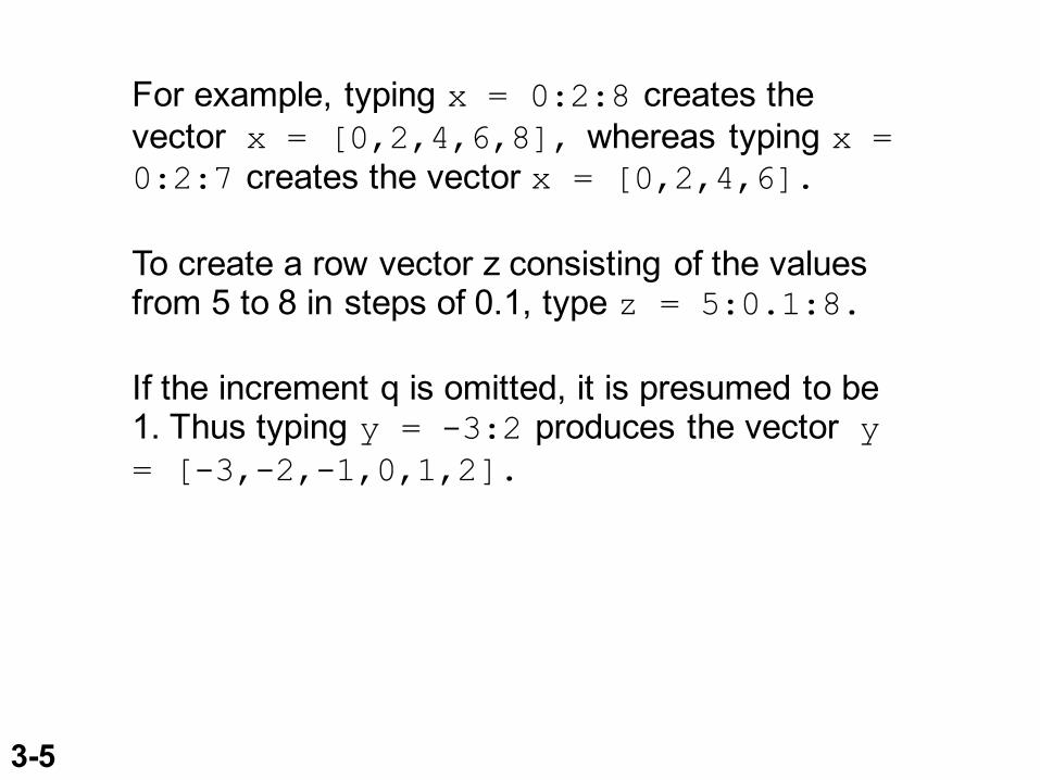
For example, typing x = 0:2:8 creates the vector x = [0,2,4,6,8], whereas typing x = 0:2:7 creates the vector x = [0,2,4,6].
To create a row vector z consisting of the values from 5 to 8 in steps of 0.1, type z = 5:0.1:8.
If the increment q is omitted, it is presumed to be 1. Thus typing y = -3:2 produces the vector y = [-3,-2,-1,0,1,2].
3-5
The linspace command also creates a linearly spaced row vector, but instead you specify the number of values rather than the increment.
The syntax is linspace(x1,x2,n), where x1 and x2are the lower and upper limits and n is the number of points.
For example, linspace(5,8,31) is equivelant to 5:0.1:8.
If n is omitted, the spacing is 1.
3-6
The logspace command creates an array of logarithmically spaced elements.
Its syntax is logspace(a,b,n), where n is the number of points between 10a and 10b.
For example, x = logspace(-1,1,1)produces the vector x = [0.1000, 1, 10.000].
If n is omitted, the number of points defaults to 50.
3-7
The logspace command creates an array of logarithmically spaced elements.
Its syntax is logspace(a,b,n), where n is the number of points between 10a and 10b.
For example, x = logspace(-1,1,4)produces the vector x = [0.1000, 0.4642, 2.1544, 10.000].
3-8
Magnitude, Length, and Absolute Value of a Vector
Keep in mind the precise meaning of these terms when using MATLAB.
The length command gives the number of elements in the vector.
The magnitude of a vector x having elements x1, x2, …, xn is a scalar, given by (x12 + x22 + … + xn2)^0.5, and is the same as the vector's geometric length.
The absolute value of a vector x is a vector whose elements are the absolute values of the elements of x.
3-9
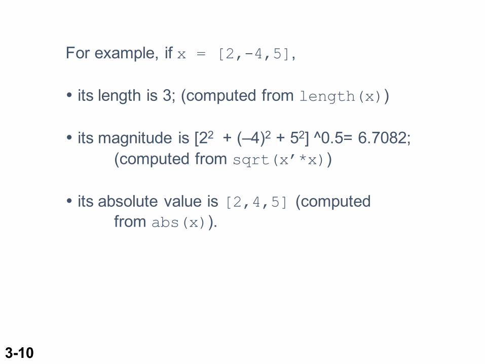
For example, if x = [2,-4,5],
• its length is 3;; (computed from length(x))
• its magnitude is [22 + (–4)2 + 52] ^0.5= 6.7082;; (computed from sqrt(x’*x))
• its absolute value is [2,4,5] (computed from abs(x)).
3-10
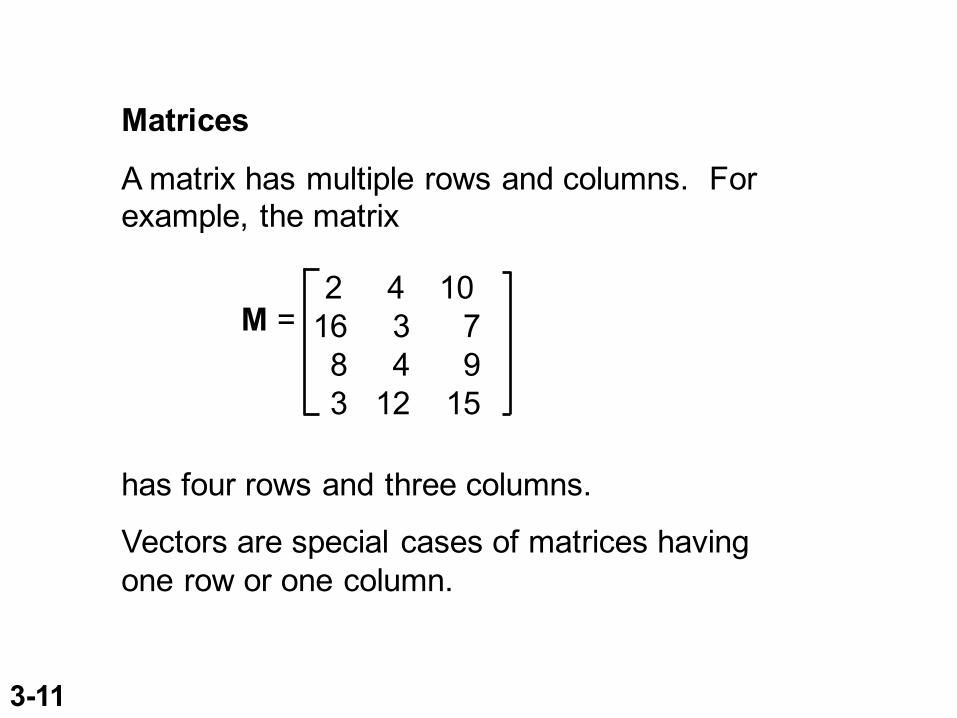
Matrices
A matrix has multiple rows and columns. For example, the matrix
has four rows and three columns.
Vectors are special cases of matrices having one row or one column.
M =2 4 10 16 3 7 8 4 9 3 12 15
3-11
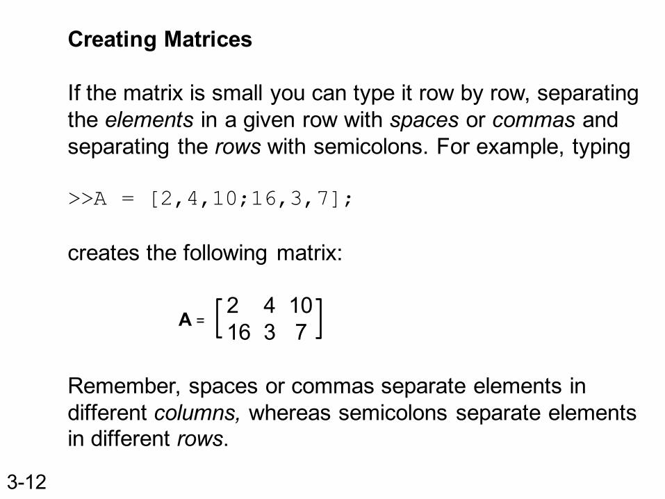
Creating Matrices
If the matrix is small you can type it row by row, separating the elements in a given row with spaces or commas and separating the rows with semicolons. For example, typing
>>A = [2,4,10;16,3,7];
creates the following matrix:
2 4 1016 3 7
Remember, spaces or commas separate elements in different columns, whereas semicolons separate elements in different rows.
A =
3-12
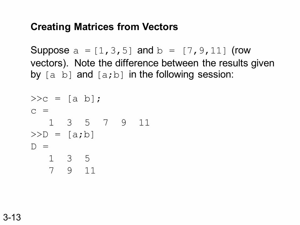
Creating Matrices from Vectors
Suppose a = [1,3,5] and b = [7,9,11] (row vectors). Note the difference between the results given by [a b] and [a;b] in the following session:
>>c = [a b];c =
1 3 5 7 9 11>>D = [a;b]D =
1 3 57 9 11
3-13
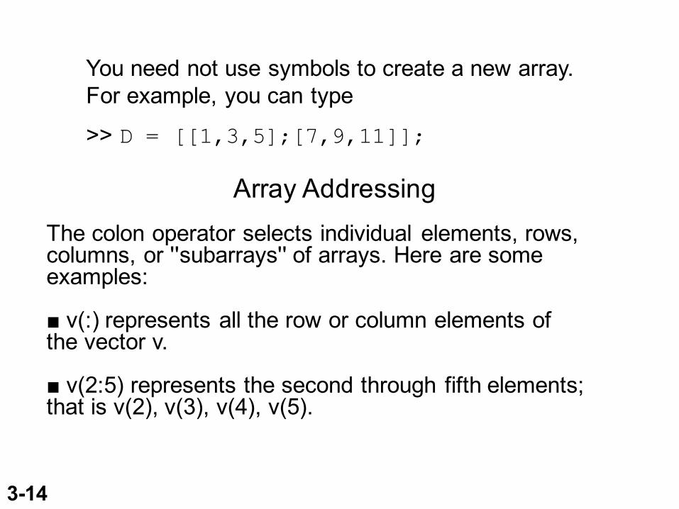
You need not use symbols to create a new array. For example, you can type
>> D = [[1,3,5];[7,9,11]];
3-14
Array AddressingThe colon operator selects individual elements, rows,columns, or ''subarrays'' of arrays. Here are some examples:
v(:) represents all the row or column elements of the vector v.
v(2:5) represents the second through fifth elements;; that is v(2), v(3), v(4), v(5).
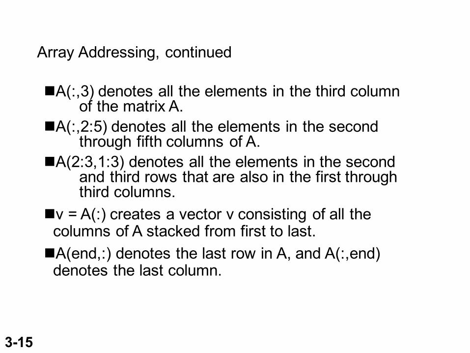
Array Addressing, continued
nA(:,3) denotes all the elements in the third column of the matrix A.
nA(:,2:5) denotes all the elements in the second through fifth columns of A.
nA(2:3,1:3) denotes all the elements in the second and third rows that are also in the first through third columns.
nv = A(:) creates a vector v consisting of all the columns of A stacked from first to last.
nA(end,:) denotes the last row in A, and A(:,end) denotes the last column.
3-15
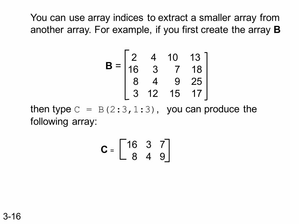
You can use array indices to extract a smaller array from another array. For example, if you first create the array B
B =
3-16
C =16 3 78 4 9
2 4 10 1316 3 7 18 8 4 9 253 12 15 17
then type C = B(2:3,1:3), you can produce the following array:
3-17
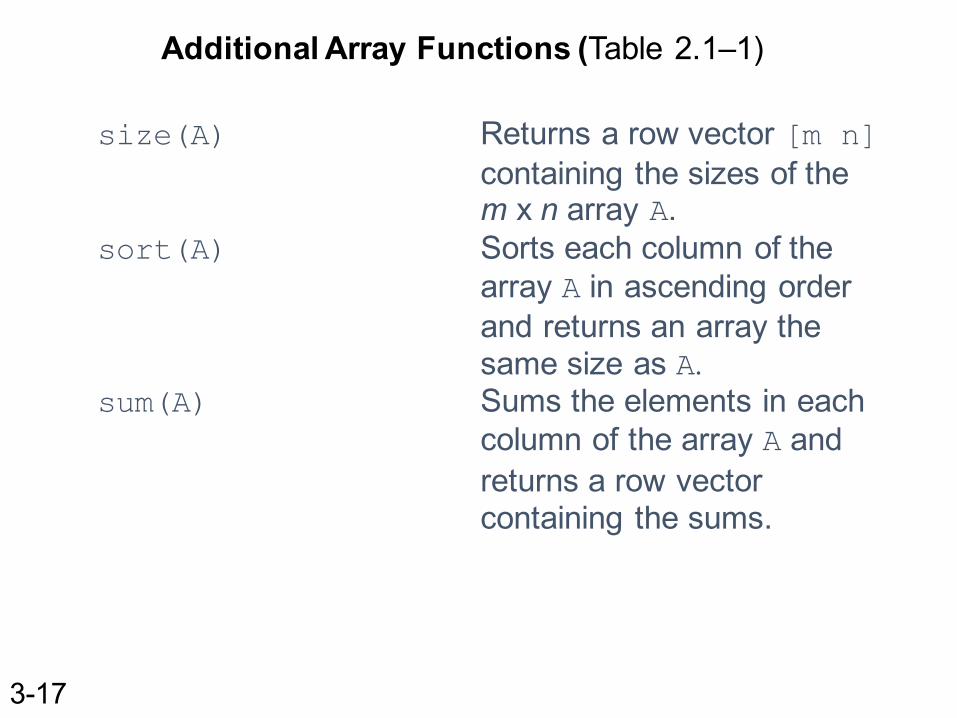
size(A) Returns a row vector [m n]containing the sizes of them x n array A.
sort(A) Sorts each column of the array A in ascending order and returns an array the same size as A.
sum(A) Sums the elements in each column of the array A andreturns a row vector containing the sums.
Additional Array Functions (Table 2.1–1)
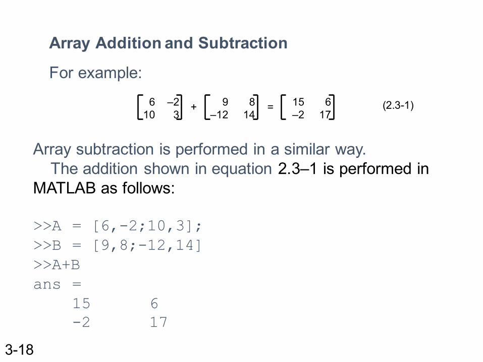
Array Addition and Subtraction
6 –210 3
+ 9 8–12 14
= 15 6–2 17
Array subtraction is performed in a similar way.The addition shown in equation 2.3–1 is performed in
MATLAB as follows:
>>A = [6,-2;10,3];>>B = [9,8;-12,14]>>A+Bans =
15 6-2 17
For example:
3-18
(2.3-1)
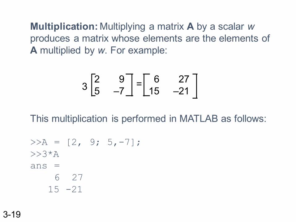
Multiplication: Multiplying a matrix A by a scalar wproduces a matrix whose elements are the elements of A multiplied by w. For example:
32 95 –7
= 6 2715 –21
This multiplication is performed in MATLAB as follows:
>>A = [2, 9; 5,-7];>>3*Aans =
6 2715 -21
3-19
Multiplication of an array by a scalar is easily defined and easily carried out.
However, multiplication of two arrays is not so straightforward.
MATLAB uses two definitions of multiplication:
(1) array multiplication (also called element-by-element multiplication), and
(2) matrix multiplication.
3-20
Division and exponentiation must also be carefully defined when you are dealing with operations between two arrays.
MATLAB has two forms of arithmetic operations on arrays. Next we introduce one form, called array operations, which are also called element-by-elementoperations. Then we will introduce matrixoperations. Each form has its own applications.
Division and exponentiation must also be carefully defined when you are dealing with operations between two arrays.
3-21
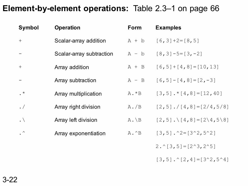
Element-by-element operations: Table 2.3–1 on page 66
Symbol
+
-
+
-
.*
./
.\
.^
Examples
[6,3]+2=[8,5]
[8,3]-5=[3,-2]
[6,5]+[4,8]=[10,13]
[6,5]-[4,8]=[2,-3]
[3,5].*[4,8]=[12,40]
[2,5]./[4,8]=[2/4,5/8]
[2,5].\[4,8]=[2\4,5\8]
[3,5].^2=[3^2,5^2]
2.^[3,5]=[2^3,2^5]
[3,5].^[2,4]=[3^2,5^4]
Operation
Scalar-array addition
Scalar-array subtraction
Array addition
Array subtraction
Array multiplication
Array right division
Array left division
Array exponentiation
Form
A + b
A – b
A + B
A – B
A.*B
A./B
A.\B
A.^B
3-22
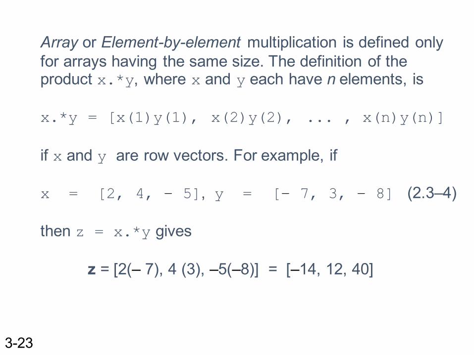
Array or Element-by-element multiplication is defined only for arrays having the same size. The definition of the product x.*y, where x and y each have n elements, is
x.*y = [x(1)y(1), x(2)y(2), ... , x(n)y(n)]
if x and y are row vectors. For example, if
x = [2, 4, – 5], y = [– 7, 3, – 8] (2.3–4)
then z = x.*y gives
z = [2(– 7), 4 (3), –5(–8)] = [–14, 12, 40]
3-23
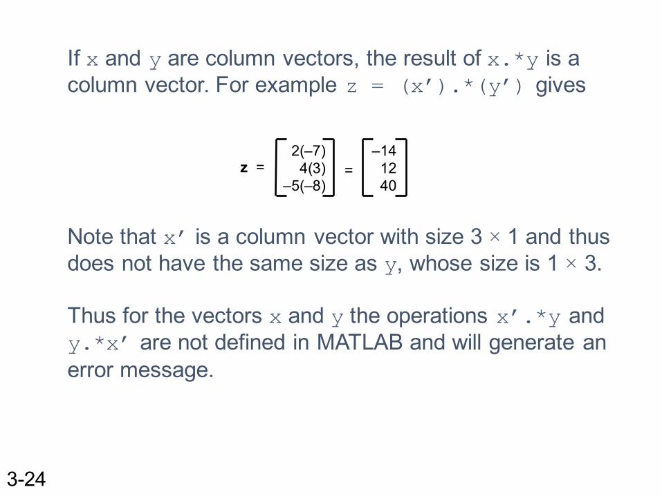
If x and y are column vectors, the result of x.*y is a column vector. For example z = (x’).*(y’) gives
Note that x’ is a column vector with size 3 × 1 and thus does not have the same size as y, whose size is 1 × 3.
Thus for the vectors x and y the operations x’.*y and y.*x’ are not defined in MATLAB and will generate an error message.
2(–7)4(3)
–5(–8)
–141240
=z =
3-24
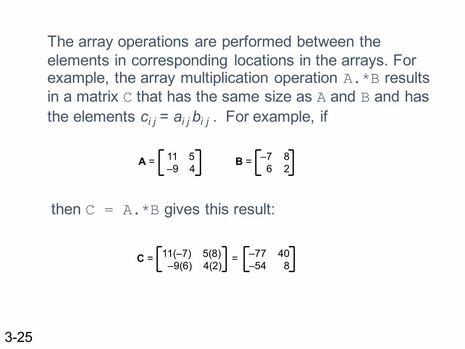
The array operations are performed between the elements in corresponding locations in the arrays. For example, the array multiplication operation A.*B results in a matrix C that has the same size as A and B and has the elements ci j = ai j bi j . For example, if
then C = A.*B gives this result:
A = 11 5–9 4
B = –7 86 2
C = 11(–7) 5(8)–9(6) 4(2)
= –77 40–54 8
3-25
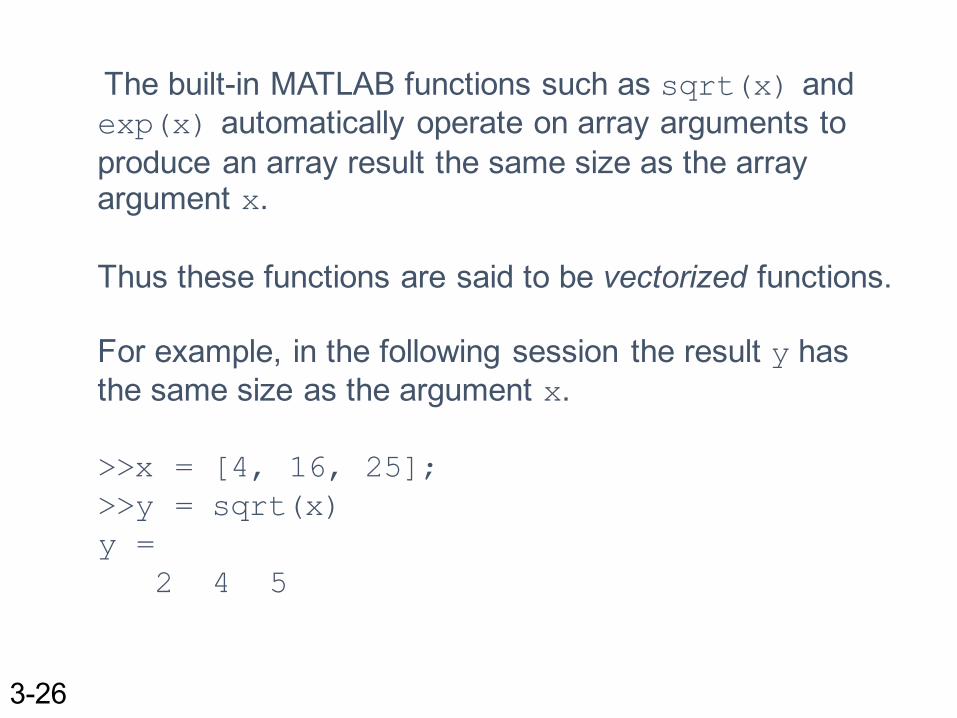
The built-in MATLAB functions such as sqrt(x) and exp(x) automatically operate on array arguments to produce an array result the same size as the array argument x.
Thus these functions are said to be vectorized functions.
For example, in the following session the result y has the same size as the argument x.
>>x = [4, 16, 25];>>y = sqrt(x)y =
2 4 5
3-26
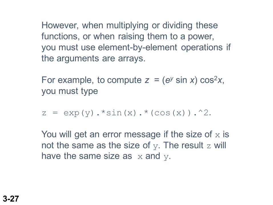
However, when multiplying or dividing these functions, or when raising them to a power, you must use element-by-element operations if the arguments are arrays.
For example, to compute z = (ey sin x) cos2x, you must type
z = exp(y).*sin(x).*(cos(x)).^2.
You will get an error message if the size of x is not the same as the size of y. The result z will have the same size as x and y.
3-27
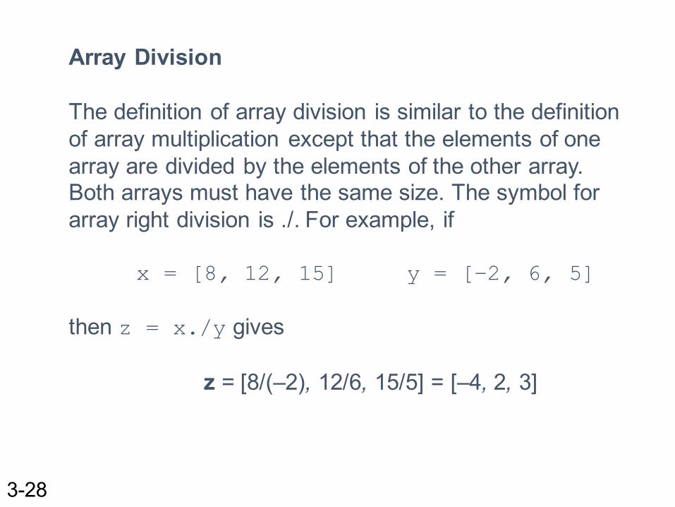
Array Division
The definition of array division is similar to the definition of array multiplication except that the elements of one array are divided by the elements of the other array. Both arrays must have the same size. The symbol for array right division is ./. For example, if
x = [8, 12, 15] y = [–2, 6, 5]
then z = x./y gives
z = [8/(–2), 12/6, 15/5] = [–4, 2, 3]
3-28
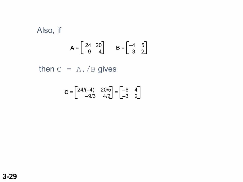
A = 24 20– 9 4
B = –4 53 2
Also, if
then C = A./B gives
C = 24/(–4) 20/5–9/3 4/2
= –6 4–3 2
3-29
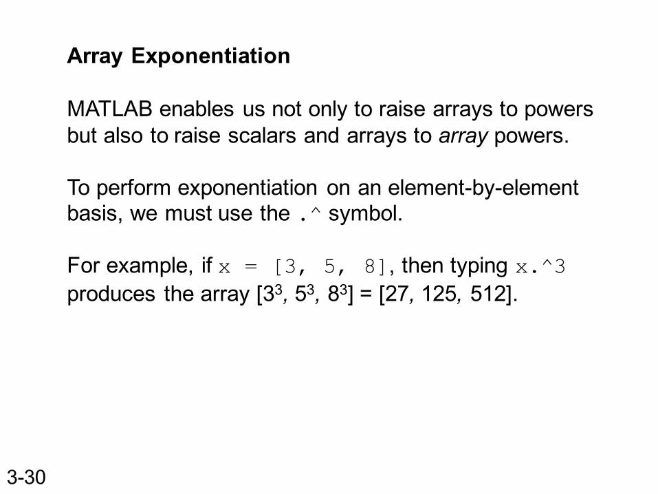
Array Exponentiation
MATLAB enables us not only to raise arrays to powers but also to raise scalars and arrays to array powers.
To perform exponentiation on an element-by-element basis, we must use the .^ symbol.
For example, if x = [3, 5, 8], then typing x.^3produces the array [33, 53, 83] = [27, 125, 512].
3-30
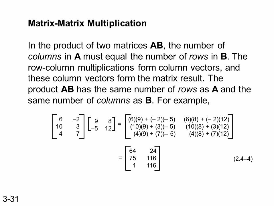
Matrix-Matrix Multiplication
In the product of two matrices AB, the number of columns in A must equal the number of rows in B. The row-column multiplications form column vectors, and these column vectors form the matrix result. The product AB has the same number of rows as A and the same number of columns as B. For example,
6 –2 10 34 7
9 8–5 12
= (6)(9) + (– 2)(– 5) (6)(8) + (– 2)(12)(10)(9) + (3)(– 5) (10)(8) + (3)(12)(4)(9) + (7)(– 5) (4)(8) + (7)(12)
64 24 75 1161 116
= (2.4–4)
3-31
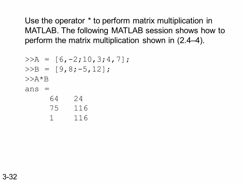
Use the operator * to perform matrix multiplication in MATLAB. The following MATLAB session shows how to perform the matrix multiplication shown in (2.4–4).
>>A = [6,-2;10,3;4,7];>>B = [9,8;-5,12];>>A*Bans =
64 2475 1161 116
3-32
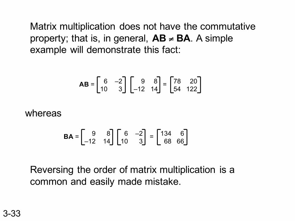
Matrix multiplication does not have the commutative property;; that is, in general, AB ≠ BA. A simple example will demonstrate this fact:
AB = 6 –210 3
9 8–12 14
= 78 2054 122
BA = 9 8–12 14
6 –210 3
= 134 668 66
whereas
Reversing the order of matrix multiplication is a common and easily made mistake.
3-33
Special MatricesTwo exceptions to the noncommutative property are the null or zero matrix, denoted by 0 and the identity, or unity, matrix, denoted by I.
The null matrix contains all zeros and is not the same as the empty matrix [ ], which has no elements.
These matrices have the following properties:
0A = A0 = 0
IA = AI = A
3-34
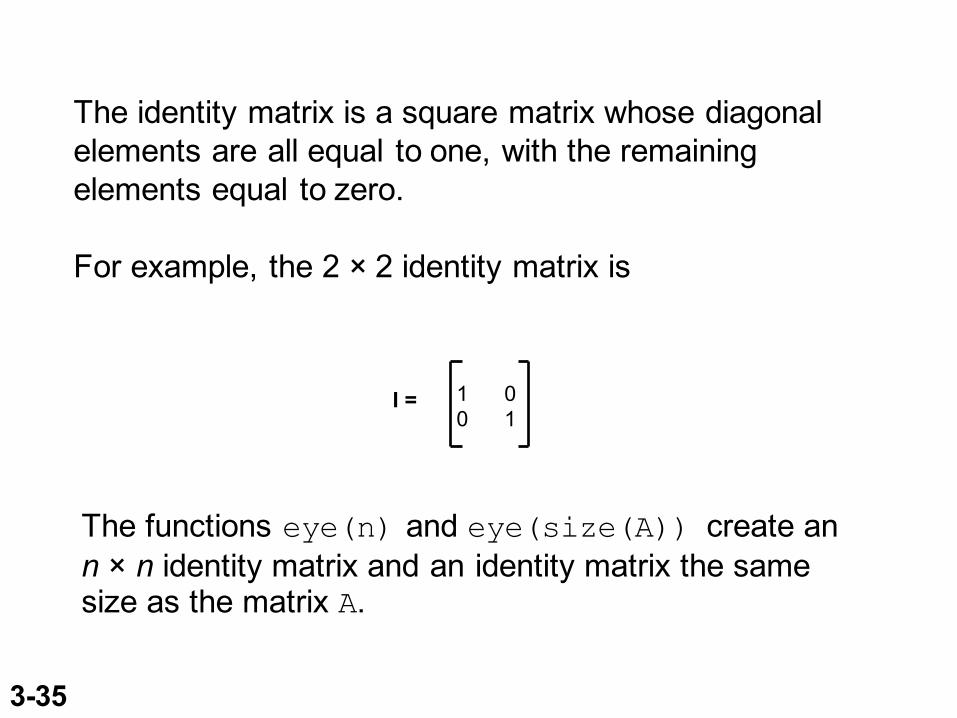
The identity matrix is a square matrix whose diagonal elements are all equal to one, with the remaining elements equal to zero.
For example, the 2 × 2 identity matrix is
I = 1 00 1
The functions eye(n) and eye(size(A)) create an n × n identity matrix and an identity matrix the same size as the matrix A.
3-35
Sometimes we want to initialize a matrix to have all zero elements. The zeros command creates a matrix of all zeros.
Typing zeros(n) creates an n × n matrix of zeros, whereas typing zeros(m,n) creates an m × n matrix of zeros.
Typing zeros(size(A)) creates a matrix of all zeros having the same dimension as the matrix A. This type of matrix can be useful for applications in which we do not know the required dimension ahead of time.
The syntax of the ones command is the same, except that it creates arrays filled with ones.
3-36
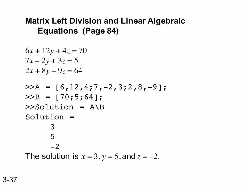
Matrix Left Division and Linear Algebraic Equations (Page 84)
6x + 12y + 4z = 707x – 2y + 3z = 52x + 8y – 9z = 64
>>A = [6,12,4;7,-2,3;2,8,-9];>>B = [70;5;64];>>Solution = A\BSolution =
35-2
The solution is x = 3, y = 5,and z = –2.
3-37