Embed Size (px)
Citation preview

Introduction toApplied Digital Control
Second Edition
Gregory P. StarrDepartment of Mechanical Engineering
The University of New Mexico
November 2006

ii
c©2006 Gregory P. Starr

Preface
This book is intended to give the senior or beginning graduate student in mechanical engineering anintroduction to digital control of mechanical systems with an emphasis on applications. The desireto write this book arose from my frustration with the existing texts on digital control, which—whilethey were exhaustive—were better suited to reference needs than for tutorial use.
While the appearance of several new texts with a more student-oriented perspective has reduced myfrustration a little, I still feel there is a need for an introductory text such as this.
MATLAB has become an almost indispensable tool in the real-world analysis and design of controlsystems, and this text includes many MATLAB scripts and examples.
My thanks go to my wife Anne, and four boys Paul, Keith, Mark, and Jeff for being patient duringthe preparation and revision of this manuscript—also my late father Duke Starr who recognized thatany kid who liked mathematics and motorcycles can’t be all bad.
Albuquerque, New MexicoNovember 2006
iii

iv PREFACE
Contents
Preface iii
1 Introduction and Scope of this Book 1
1.1 Continuous and Digital Control . . . . . . . . . . . . . . . . . . . . . . . . . . . . . . 1
1.1.1 Feedback control . . . . . . . . . . . . . . . . . . . . . . . . . . . . . . . . . . 1
1.1.2 Digital control . . . . . . . . . . . . . . . . . . . . . . . . . . . . . . . . . . . 2
1.2 Philosophy and Text Coverage . . . . . . . . . . . . . . . . . . . . . . . . . . . . . . 4
2 Linear Discrete Systems and the Z-Transform 7
2.1 Chapter Overview . . . . . . . . . . . . . . . . . . . . . . . . . . . . . . . . . . . . . 7
2.2 Linear Difference Equations . . . . . . . . . . . . . . . . . . . . . . . . . . . . . . . . 8
2.2.1 Solving Difference Equations . . . . . . . . . . . . . . . . . . . . . . . . . . . 9
2.3 The Z-Transform and the Discrete Transfer Function . . . . . . . . . . . . . . . . . . 11
2.3.1 The z-Transform . . . . . . . . . . . . . . . . . . . . . . . . . . . . . . . . . . 11
2.3.2 Discrete Transfer Function . . . . . . . . . . . . . . . . . . . . . . . . . . . . 11
2.3.3 Block Diagrams of Discrete Systems . . . . . . . . . . . . . . . . . . . . . . . 13
2.3.4 Going From Transfer Function to Difference Equation . . . . . . . . . . . . . 14
2.3.5 Relation of the Transfer Function to the Unit Pulse Response . . . . . . . . . 15
2.4 Dynamic Response of Discrete Systems . . . . . . . . . . . . . . . . . . . . . . . . . . 16
2.4.1 Unit step . . . . . . . . . . . . . . . . . . . . . . . . . . . . . . . . . . . . . . 17
2.4.2 Exponential . . . . . . . . . . . . . . . . . . . . . . . . . . . . . . . . . . . . . 17
v
vi CONTENTS
2.4.3 Damped Sinusoid . . . . . . . . . . . . . . . . . . . . . . . . . . . . . . . . . . 18
2.4.4 Relationship between z-plane poles and transient response . . . . . . . . . . . 20
2.4.5 Effect of Zeros on Dynamic Response . . . . . . . . . . . . . . . . . . . . . . 21
2.5 Correspondence between Discrete and Continuous Signals . . . . . . . . . . . . . . . 21
2.6 Frequency Response of Discrete Systems . . . . . . . . . . . . . . . . . . . . . . . . . 23
2.7 Z-Transform Properties . . . . . . . . . . . . . . . . . . . . . . . . . . . . . . . . . . 24
2.7.1 Inverse Transforming . . . . . . . . . . . . . . . . . . . . . . . . . . . . . . . . 26
2.8 A Word about LTI Systems and MATLAB functions . . . . . . . . . . . . . . . . . . 30
2.8.1 LTI Systems . . . . . . . . . . . . . . . . . . . . . . . . . . . . . . . . . . . . 30
2.8.2 Overloaded Functions . . . . . . . . . . . . . . . . . . . . . . . . . . . . . . . 31
2.9 Table of Z-Transforms . . . . . . . . . . . . . . . . . . . . . . . . . . . . . . . . . . . 32
3 Discrete Simulation of Continuous Systems 35
3.1 Chapter Overview . . . . . . . . . . . . . . . . . . . . . . . . . . . . . . . . . . . . . 35
3.2 Discrete Simulation using Numerical Integration . . . . . . . . . . . . . . . . . . . . 36
3.2.1 Forward rectangular rule (Euler’s rule) . . . . . . . . . . . . . . . . . . . . . . 37
3.2.2 Backward rectangular rule . . . . . . . . . . . . . . . . . . . . . . . . . . . . . 38
3.2.3 Trapezoidal rule . . . . . . . . . . . . . . . . . . . . . . . . . . . . . . . . . . 38
3.2.4 Prewarped trapezoidal rule . . . . . . . . . . . . . . . . . . . . . . . . . . . . 41
3.3 Pole-Zero Mapping . . . . . . . . . . . . . . . . . . . . . . . . . . . . . . . . . . . . . 44
3.4 Comparison of Simulations . . . . . . . . . . . . . . . . . . . . . . . . . . . . . . . . 45
3.5 Using MATLAB in Discrete Simulation . . . . . . . . . . . . . . . . . . . . . . . . . 46
3.5.1 Finding transfer function from LTI system . . . . . . . . . . . . . . . . . . . . 49
3.6 Implementation of Difference Equations in Real Time . . . . . . . . . . . . . . . . . 49
3.6.1 Direct realization . . . . . . . . . . . . . . . . . . . . . . . . . . . . . . . . . . 50
3.6.2 Canonical realization . . . . . . . . . . . . . . . . . . . . . . . . . . . . . . . . 50
CONTENTS vii
4 Sampled Data Systems 55
4.1 Introduction . . . . . . . . . . . . . . . . . . . . . . . . . . . . . . . . . . . . . . . . . 55
4.2 The Sampling Process as Impulse Modulation . . . . . . . . . . . . . . . . . . . . . . 55
4.3 Frequency Spectra of Sampled Signals—Aliasing . . . . . . . . . . . . . . . . . . . . 58
4.3.1 Fourier transform and Fourier series . . . . . . . . . . . . . . . . . . . . . . . 58
4.4 Desampling or Signal Reconstruction . . . . . . . . . . . . . . . . . . . . . . . . . . . 62
4.4.1 Impulse response of the Ideal Desampling Filter . . . . . . . . . . . . . . . . 62
4.4.2 The ZOH as a Desampling Filter . . . . . . . . . . . . . . . . . . . . . . . . . 64
4.5 Block Diagram Analysis . . . . . . . . . . . . . . . . . . . . . . . . . . . . . . . . . . 66
4.5.1 Two blocks with a sampler between them . . . . . . . . . . . . . . . . . . . . 67
4.5.2 Two blocks without a sampler between them . . . . . . . . . . . . . . . . . . 69
4.5.3 Response between samples . . . . . . . . . . . . . . . . . . . . . . . . . . . . . 72
5 Design Using Transform Methods 75
5.1 Introduction . . . . . . . . . . . . . . . . . . . . . . . . . . . . . . . . . . . . . . . . . 75
5.2 Example System and Specifications . . . . . . . . . . . . . . . . . . . . . . . . . . . . 76
5.2.1 Steady-State Accuracy . . . . . . . . . . . . . . . . . . . . . . . . . . . . . . . 78
5.2.2 Transient Response . . . . . . . . . . . . . . . . . . . . . . . . . . . . . . . . . 80
5.2.3 Disturbance Rejection . . . . . . . . . . . . . . . . . . . . . . . . . . . . . . . 84
5.2.4 Control Effort and Gain Distribution . . . . . . . . . . . . . . . . . . . . . . . 85
5.2.5 Parameter Sensitivity . . . . . . . . . . . . . . . . . . . . . . . . . . . . . . . 85
5.3 Design in the s plane by Discrete Equivalent . . . . . . . . . . . . . . . . . . . . . . 85
5.4 Direct Design in the z Plane . . . . . . . . . . . . . . . . . . . . . . . . . . . . . . . . 89
5.5 Another Design Example . . . . . . . . . . . . . . . . . . . . . . . . . . . . . . . . . 95
5.6 Modeling using Simulink . . . . . . . . . . . . . . . . . . . . . . . . . . . . . . . . . . 104
5.6.1 Creating the Simulink Model . . . . . . . . . . . . . . . . . . . . . . . . . . . 105
5.7 PID Control (Mode Controllers) . . . . . . . . . . . . . . . . . . . . . . . . . . . . . 107
5.7.1 Proportional Control . . . . . . . . . . . . . . . . . . . . . . . . . . . . . . . . 107
viii CONTENTS
5.7.2 Derivative Action . . . . . . . . . . . . . . . . . . . . . . . . . . . . . . . . . . 108
5.7.3 Integral Action . . . . . . . . . . . . . . . . . . . . . . . . . . . . . . . . . . . 108
5.7.4 PD Control . . . . . . . . . . . . . . . . . . . . . . . . . . . . . . . . . . . . . 108
5.7.5 PI Control . . . . . . . . . . . . . . . . . . . . . . . . . . . . . . . . . . . . . 109
5.7.6 PID Control . . . . . . . . . . . . . . . . . . . . . . . . . . . . . . . . . . . . 109
6 State-Space Analysis of Continuous Systems 113
6.1 Introduction . . . . . . . . . . . . . . . . . . . . . . . . . . . . . . . . . . . . . . . . . 113
6.2 System Description . . . . . . . . . . . . . . . . . . . . . . . . . . . . . . . . . . . . . 114
6.2.1 State Equation and Output Equation . . . . . . . . . . . . . . . . . . . . . . 114
6.2.2 State equation from Transfer Function . . . . . . . . . . . . . . . . . . . . . . 116
6.2.3 Transfer Function from State-Variable Description . . . . . . . . . . . . . . . 116
6.3 Different State-Space Representations . . . . . . . . . . . . . . . . . . . . . . . . . . 117
6.3.1 State Variable Transformation . . . . . . . . . . . . . . . . . . . . . . . . . . 118
6.3.2 Control Canonical Form . . . . . . . . . . . . . . . . . . . . . . . . . . . . . . 118
6.3.3 Diagonal (modal or decoupled) Form . . . . . . . . . . . . . . . . . . . . . . . 120
6.4 MATLAB Tools . . . . . . . . . . . . . . . . . . . . . . . . . . . . . . . . . . . . . . . 121
6.4.1 Transform↔State-Space . . . . . . . . . . . . . . . . . . . . . . . . . . . . . . 121
6.4.2 Eigenvalues, Eigenvectors, Diagonalization . . . . . . . . . . . . . . . . . . . . 123
6.4.3 Dynamic Response of State-Space Forms . . . . . . . . . . . . . . . . . . . . 125
7 Digital Controller Design using State Space Methods 129
7.1 Introduction . . . . . . . . . . . . . . . . . . . . . . . . . . . . . . . . . . . . . . . . . 129
7.2 Canonical State-Space Forms from Transfer Function . . . . . . . . . . . . . . . . . . 129
7.3 Solution to the State Equation . . . . . . . . . . . . . . . . . . . . . . . . . . . . . . 131
7.3.1 Homogeneous solution . . . . . . . . . . . . . . . . . . . . . . . . . . . . . . . 132
7.3.2 Particular solution . . . . . . . . . . . . . . . . . . . . . . . . . . . . . . . . . 133
7.3.3 Calculating system and output matrices . . . . . . . . . . . . . . . . . . . . . 134

CONTENTS ix
7.4 Control Law Design . . . . . . . . . . . . . . . . . . . . . . . . . . . . . . . . . . . . 135
7.4.1 Pole Placement . . . . . . . . . . . . . . . . . . . . . . . . . . . . . . . . . . . 135
7.4.2 Selecting System Pole Locations . . . . . . . . . . . . . . . . . . . . . . . . . 138
7.4.3 Controllability and the Control Canonical Form . . . . . . . . . . . . . . . . . 138
7.4.4 Ackermann’s Rule and a Test for Controllability . . . . . . . . . . . . . . . . 139
7.4.5 MATLAB Tools . . . . . . . . . . . . . . . . . . . . . . . . . . . . . . . . . . 141
7.4.6 Poles and Zeros . . . . . . . . . . . . . . . . . . . . . . . . . . . . . . . . . . . 142
7.4.7 More on Controllability . . . . . . . . . . . . . . . . . . . . . . . . . . . . . . 143
7.5 State Estimator Design . . . . . . . . . . . . . . . . . . . . . . . . . . . . . . . . . . 144
7.5.1 Prediction Estimator . . . . . . . . . . . . . . . . . . . . . . . . . . . . . . . . 144
7.5.2 Observability and Ackermann’s Formula . . . . . . . . . . . . . . . . . . . . . 146
7.5.3 MATLAB Tools . . . . . . . . . . . . . . . . . . . . . . . . . . . . . . . . . . 146
7.6 Regulator: Control Law plus Estimator . . . . . . . . . . . . . . . . . . . . . . . . . 147
7.6.1 Controller Transfer Function . . . . . . . . . . . . . . . . . . . . . . . . . . . 154
7.7 Current and Reduced-Order Estimators . . . . . . . . . . . . . . . . . . . . . . . . . 156
7.7.1 Current Estimator . . . . . . . . . . . . . . . . . . . . . . . . . . . . . . . . . 157
7.7.2 Reduced-Order Estimators . . . . . . . . . . . . . . . . . . . . . . . . . . . . 159
7.8 Adding a Reference Input . . . . . . . . . . . . . . . . . . . . . . . . . . . . . . . . . 161
7.8.1 Reference Input with Full State Feedback . . . . . . . . . . . . . . . . . . . . 161
7.8.2 Reference Input with an Estimator . . . . . . . . . . . . . . . . . . . . . . . . 164
7.9 Uniqueness of Solution—The MIMO Case . . . . . . . . . . . . . . . . . . . . . . . . 165
7.10 Another Example—Stick Balancer . . . . . . . . . . . . . . . . . . . . . . . . . . . . 166
8 System Identification 173
8.1 Introduction . . . . . . . . . . . . . . . . . . . . . . . . . . . . . . . . . . . . . . . . . 173
8.2 Models and Data Organization . . . . . . . . . . . . . . . . . . . . . . . . . . . . . . 173
8.3 Least Squares Approximations . . . . . . . . . . . . . . . . . . . . . . . . . . . . . . 175
8.3.1 Minimization of ε2 by Calculus . . . . . . . . . . . . . . . . . . . . . . . . . . 175
x CONTENTS
8.3.2 Minimization of ε2 by Linear Algebra . . . . . . . . . . . . . . . . . . . . . . 176
8.4 Application to System Identification . . . . . . . . . . . . . . . . . . . . . . . . . . . 176
8.5 Practical Issues—How Well Does it Work? . . . . . . . . . . . . . . . . . . . . . . . . 177
8.5.1 Selection of Input . . . . . . . . . . . . . . . . . . . . . . . . . . . . . . . . . 177
8.5.2 Quantization Noise . . . . . . . . . . . . . . . . . . . . . . . . . . . . . . . . . 178
8.5.3 Identification Example . . . . . . . . . . . . . . . . . . . . . . . . . . . . . . . 180

List of Figures
1.1 Basic digital control system. . . . . . . . . . . . . . . . . . . . . . . . . . . . . . . . . 2
1.2 Three types of signals. . . . . . . . . . . . . . . . . . . . . . . . . . . . . . . . . . . . 3
2.1 A/D converter and computer . . . . . . . . . . . . . . . . . . . . . . . . . . . . . . . 8
2.2 Numerical integration. . . . . . . . . . . . . . . . . . . . . . . . . . . . . . . . . . . . 10
2.3 Block diagram of trapezoidal integration. . . . . . . . . . . . . . . . . . . . . . . . . 14
2.4 Unit step pole/zero locations and response. . . . . . . . . . . . . . . . . . . . . . . . 17
2.5 Exponential pole/zero locations and response. . . . . . . . . . . . . . . . . . . . . . . 18
2.6 Discrete damped sinusoidal response. . . . . . . . . . . . . . . . . . . . . . . . . . . . 20
2.7 Contours in s and z planes. . . . . . . . . . . . . . . . . . . . . . . . . . . . . . . . . 23
2.8 Step response of discrete system. . . . . . . . . . . . . . . . . . . . . . . . . . . . . . 29
3.1 Forward integration rule. . . . . . . . . . . . . . . . . . . . . . . . . . . . . . . . . . . 38
3.2 Backward integration rule. . . . . . . . . . . . . . . . . . . . . . . . . . . . . . . . . . 39
3.3 Trapezoidal integration rule. . . . . . . . . . . . . . . . . . . . . . . . . . . . . . . . . 40
3.4 Left-half s-plane mapped into z-plane. . . . . . . . . . . . . . . . . . . . . . . . . . . 41
3.5 Bode magnitude plots. . . . . . . . . . . . . . . . . . . . . . . . . . . . . . . . . . . . 46
3.6 Bode angle plots. . . . . . . . . . . . . . . . . . . . . . . . . . . . . . . . . . . . . . . 47
3.7 Observer canonical block diagram realization. . . . . . . . . . . . . . . . . . . . . . . 51
4.1 Convolution of continuous signal with impulse train. . . . . . . . . . . . . . . . . . . 56
xi

xii LIST OF FIGURES
4.2 Sampler and zero-order hold. . . . . . . . . . . . . . . . . . . . . . . . . . . . . . . . 57
4.3 Frequency spectra of two signals. . . . . . . . . . . . . . . . . . . . . . . . . . . . . . 61
4.4 Plot of two sinusoids which have identical values at the sampling intervals: an exampleof aliasing. . . . . . . . . . . . . . . . . . . . . . . . . . . . . . . . . . . . . . . . . . . 62
4.5 Use of ideal desampling filter. . . . . . . . . . . . . . . . . . . . . . . . . . . . . . . . 63
4.6 Sinc function. . . impulse response of ideal desampling filter. . . . . . . . . . . . . . . 64
4.7 Frequency response of zero-order hold. . . . . . . . . . . . . . . . . . . . . . . . . . . 65
4.8 Repeated spectra and attenuation by ZOH. . . . . . . . . . . . . . . . . . . . . . . . 67
5.1 Block diagram of antenna plant. . . . . . . . . . . . . . . . . . . . . . . . . . . . . . 77
5.2 Another block diagram of antenna plant. . . . . . . . . . . . . . . . . . . . . . . . . . 77
5.3 Block diagram for ss error analysis. . . . . . . . . . . . . . . . . . . . . . . . . . . . . 78
5.4 Transient response specifications, showing percent overshoot PO, rise time tr, andsettling time ts . . . . . . . . . . . . . . . . . . . . . . . . . . . . . . . . . . . . . . . 81
5.5 Regions in the s-plane corresponding to restrictions on PO, tr, and ts. . . . . . . . . 83
5.6 Regions in the z-plane corresponding to restrictions on PO ≤ 15%, tr ≤ 6 sec, andts ≤ 20 sec. (Sampling period T = 1 seconds was chosen to obtain the tr and ts regions) 84
5.7 Root Locus of the antenna plant with D(s) compensator. . . . . . . . . . . . . . . . 87
5.8 Unit Step Response of the Continuous Antenna Controller Design . . . . . . . . . . . 88
5.9 Unit Step Response of the Actual Discrete Antenna Controller Design using the D(z)designed in the Continuous Domain. . . . . . . . . . . . . . . . . . . . . . . . . . . . 90
5.10 Root Locus of antenna system vs proportional gain K. . . . . . . . . . . . . . . . . . 91
5.11 Root Locus of antenna system vs gain K using compensator D(z). . . . . . . . . . . 92
5.12 Step response of system designed in z plane. . . . . . . . . . . . . . . . . . . . . . . . 93
5.13 Unit step response of plant G(s). . . . . . . . . . . . . . . . . . . . . . . . . . . . . . 95
5.14 Acceptable regions for poles. . . . . . . . . . . . . . . . . . . . . . . . . . . . . . . . 97
5.15 Hand sketch of root locus for Example 2. . . . . . . . . . . . . . . . . . . . . . . . . 99
5.16 MATLAB root locus for Example 2. . . . . . . . . . . . . . . . . . . . . . . . . . . . 100
5.17 Unit step response of closed-loop system for Example 2. . . . . . . . . . . . . . . . . 102

LIST OF FIGURES xiii
5.18 Control force u(t) for unit step r(t) in Example 2. . . . . . . . . . . . . . . . . . . . 104
5.19 Block diagram for Simulink model. . . . . . . . . . . . . . . . . . . . . . . . . . . . . 105
5.20 Block diagram of the finished Simulink model. . . . . . . . . . . . . . . . . . . . . . . 105
5.21 Simulink screenshot showing plots. . . . . . . . . . . . . . . . . . . . . . . . . . . . . 106
5.22 PID control action . . . . . . . . . . . . . . . . . . . . . . . . . . . . . . . . . . . . . 107
5.23 A ball suspended by an electromagnet. . . . . . . . . . . . . . . . . . . . . . . . . . . 110
5.24 An automotive cruise-control system. . . . . . . . . . . . . . . . . . . . . . . . . . . . 111
6.1 Control system design. . . . . . . . . . . . . . . . . . . . . . . . . . . . . . . . . . . . 114
6.2 Spring-mass-damper system. . . . . . . . . . . . . . . . . . . . . . . . . . . . . . . . . 115
6.3 Control Canonical Form. . . . . . . . . . . . . . . . . . . . . . . . . . . . . . . . . . . 119
6.4 DC motor driving inertia. . . . . . . . . . . . . . . . . . . . . . . . . . . . . . . . . . 126
6.5 Coupled spring-mass system. . . . . . . . . . . . . . . . . . . . . . . . . . . . . . . . 127
7.1 Control Canonical Form. . . . . . . . . . . . . . . . . . . . . . . . . . . . . . . . . . . 130
7.2 Response of controlled inertia plant from initial condition x(0) = [1 1]T . . . . . . . 138
7.3 Dual pendula on cart. . . . . . . . . . . . . . . . . . . . . . . . . . . . . . . . . . . . 140
7.4 Open-loop estimator. . . . . . . . . . . . . . . . . . . . . . . . . . . . . . . . . . . . . 145
7.5 Closed-loop estimator. . . . . . . . . . . . . . . . . . . . . . . . . . . . . . . . . . . . 145
7.6 Control law plus estimator. . . . . . . . . . . . . . . . . . . . . . . . . . . . . . . . . 147
7.7 Response of undamped harmonic oscillator from initial state. . . . . . . . . . . . . . 148
7.8 Response of controlled plant from initial state. . . . . . . . . . . . . . . . . . . . . . 150
7.9 y response of plant + control law + estimator from initial state (1, 1, 1, 0). . . . . . . 152
7.10 Estimator error response. . . . . . . . . . . . . . . . . . . . . . . . . . . . . . . . . . 153
7.11 Root locus of oscillator plant and controller. . . . . . . . . . . . . . . . . . . . . . . . 156
7.12 Block diagram of reference input added to plant with full state feedback. . . . . . . . 161
7.13 Reference input added to plant with full state feedback plus feedforward. . . . . . . 162
7.14 Reference input added to plant with estimator. . . . . . . . . . . . . . . . . . . . . . 164

xiv LIST OF FIGURES
7.15 Pendulum and cart driven by position servo. . . . . . . . . . . . . . . . . . . . . . . 166
7.16 Response of pendulum to 1 cm step servo displacement. . . . . . . . . . . . . . . . . 168
7.17 Response of cart and pendulum to 1 cm initial condition of cart (note initial motionof cart is away from equilibrium). . . . . . . . . . . . . . . . . . . . . . . . . . . . . . 170
7.18 Response of cart and pendulum to reference trajectory of 0.2 m in 1 second at constantvelocity. . . . . . . . . . . . . . . . . . . . . . . . . . . . . . . . . . . . . . . . . . . . 171
8.1 Normally-distributed random noise with mean 0.0 and variance 1.0. . . . . . . . . . 179
8.2 Random binary signal. . . . . . . . . . . . . . . . . . . . . . . . . . . . . . . . . . . . 179
8.3 Effect of rounding with q = 1. . . . . . . . . . . . . . . . . . . . . . . . . . . . . . . . 180
8.4 Quantized output of example G(z) driven by random binary signal. . . . . . . . . . . 181
8.5 Comparison of actual and model step responses. . . . . . . . . . . . . . . . . . . . . 182

Chapter 1
Introduction and Scope of thisBook
This book is intended to give the student an introduction to the field of digital control, with anemphasis on applications. Both transform-based and state-variable approaches will be included,with a brief introduction to system identification.
The material requires some understanding of the Laplace transform and assumes that the readerhas studied linear feedback control systems.
1.1 Continuous and Digital Control
1.1.1 Feedback control
The study of feedback control systems is concerned with using a measurement of the output of aplant (device to be controlled) to modify its input. The controller is that part of the system thatreceives the measurement of the plant output, then generates the plant input, hence closing the loop.Control system design is the task of designing this controller such that the closed-loop system hassatisfactory performance. Broadly speaking, some goals of most closed-loop control systems are:
• Command Tracking . . . cause the output to track the reference input closely
• Disturbance Rejection . . . isolate the output from unwanted disturbance inputs
• Parameter Sensitivity . . . reduce the effect on the output of variations in plant parameters
These are goals of both continuous and digital control systems.
1
2 CHAPTER 1. INTRODUCTION AND SCOPE OF THIS BOOK
Computer+ -
A/D
Clock
D/A Plant
Sensor
r (t) e(t) e(kT ) u(kT ) u(t)
w(t)
y(t)
v(t )
y(t)
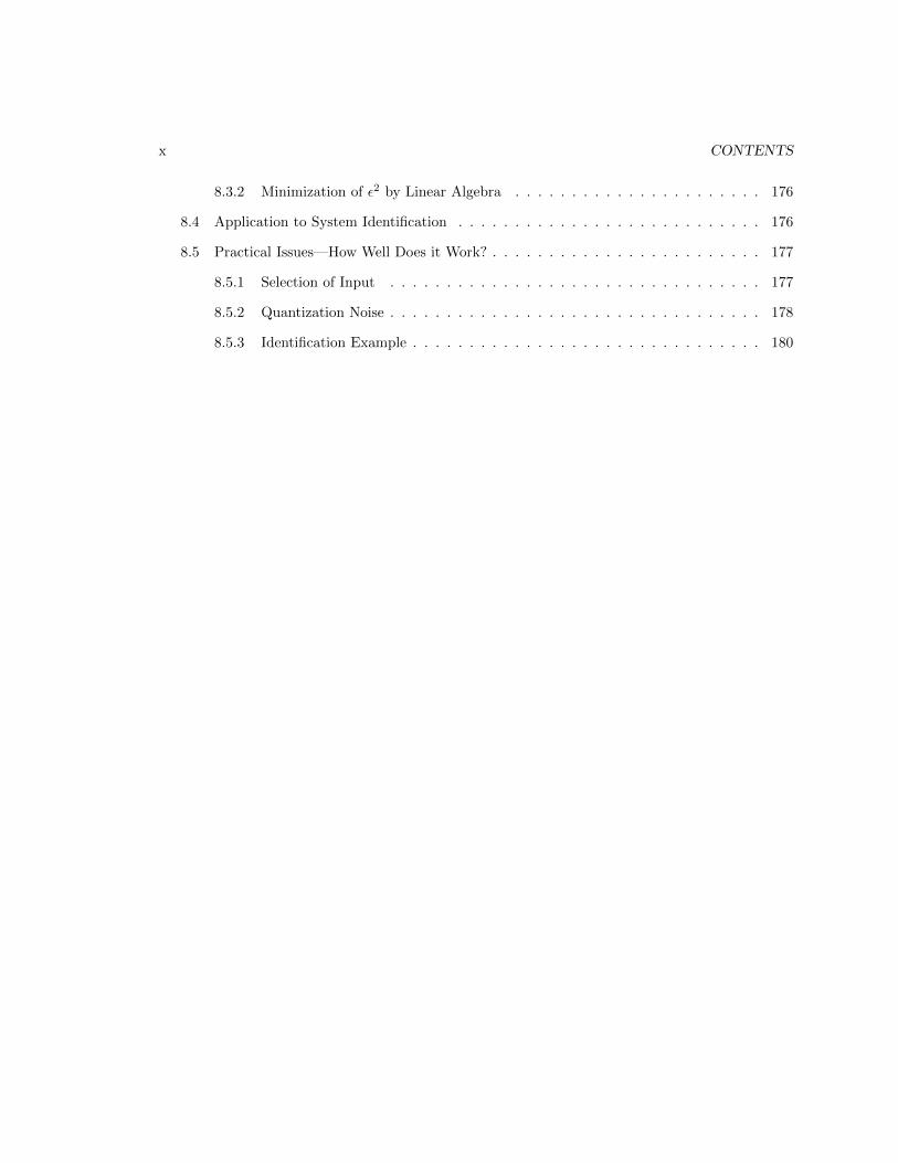
r = reference input or setpointu = control force (actuator input)y = controlled variable or outputy = measurement of controlled variablee = r − y = error signalw = disturbance acting on the plantv = measurement noiseA/D = analog-to-digital converterD/A = digital-to-analog converter
Figure 1.1: Basic digital control system.
1.1.2 Digital control
Digital control systems employ a computer as a fundamental component in the controller. Thecomputer typically receives a measurement of the controlled variable, also often receives the referenceinput, and produces its output using an algorithm. This output is usually converted to an analogsignal using a D/A converter, then amplified by a power amplifier to drive the plant. A blockdiagram of a typical digital control system is shown in Figure 1.1.
When compared to a continuous-time system, there are three new elements in the block diagram ofFigure 1.1:
• A/D converter. This device acts on a continuous physical variable, typically a voltage, andconverts it into an integer number. A/D converters typically have unipolar ranges of 0–5 V,0–10 V, or bipolar ranges of ± 5 V, or ± 10 V. These are often jumper-selectable. The A/Dconversion causes quantization q, given by the resolution of the converter in bits. Commonresolutions are 8 bits (256 levels), and 12 bits (4096 levels). A 12-bit A/D converter of range±10 volts would have a conversion quantum of q = 20/4096 = 4.88 mV. Note that quantization
1.1. CONTINUOUS AND DIGITAL CONTROL 3
is a nonlinear operation. The effect of quantization on a continuous signal is often calledquantization noise.
• D/A converter. This device converts an (integer) number to a voltage. The voltage rangesand converter resolutions are the same as for the A/D converter. A D/A converter functionsas a zero-order hold, holding its output at a constant value until it receives the next discreteinput.
• Sampling. This is represented by the clock in Figure 1.1. The computer samples the error (orit may sample both the setpoint and the measurement, thus forming the error internally) atparticular times. In this book we will assume that sampling is at a constant period T , whichis called the sampling period. The sampling frequency in Hz is 1/T . When a continuous signale(t) has been sampled, it is called a discrete signal and is denoted by e(kT ) or e(k) or ek.Discrete signals are only mathematically defined at the sample instants tk = kT .
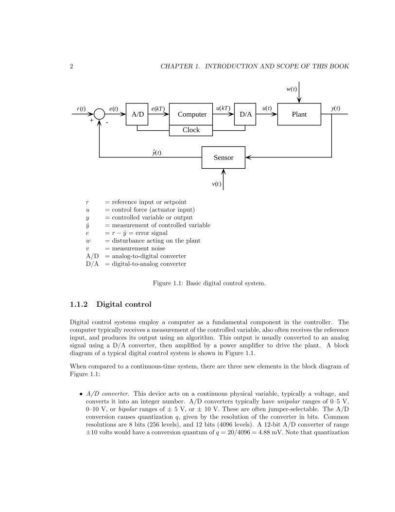
A system in which there are only discrete signals is called a discrete-time system. Systems with bothcontinuous and discrete variables are called sampled-data systems. When quantization is added, thesystem may be called digital. Continuous, discrete, and “zero-order hold” (output of D/A) signalsare shown in Figure 1.2, where the signal is sin(t).
0 1 2 3 4 5 6 7 8 9 10-1
0
1Continuous
0 1 2 3 4 5 6 7 8 9 10-1
0
1Discrete
0 1 2 3 4 5 6 7 8 9 10-1
0
1
Time (seconds)
Output of D/A
Each sample is discretized
Sample held for one period
Figure 1.2: Three types of signals.
4 CHAPTER 1. INTRODUCTION AND SCOPE OF THIS BOOK
Much of the task of designing a digital controller is in accounting for the effects of quantizationand sampling, especially sampling. If both T and q are small, digital signals approach continuoussignals, and continuous methods of analysis and design may be used. However, when this is not thecase, continuous methods can lead to erroneous results.
1.2 Philosophy and Text Coverage
The philosophy of this course is to present the basic material necessary for the analysis and designof digital control systems. We assume a background in continuous systems, and relate the digitalproblem to its continuous counterpart. The emphasis is on understanding the physical reality behindthe analysis.
The eight chapters in this book contain the following material:
Chapter 1. This chapter. Describes philosophy and content of book. Some definitions. Rationalefor studying digital control.
Chapter 2. Sampled (discrete-time) variables. Introduction of the z-transform for discrete vari-ables, which is analogous to the Laplace transform for continuous variables.
Chapter 3. Discrete simulations of continuous systems. Several methods of simulation are given,specifically numerical integration, pole-zero mapping, and zero-order hold equivalence.
Chapter 4. Frequency spectra of sampled signals. The impulse modulation model of sampling.Aliasing and its effects.
Chapter 5. Transform-based design of digital control systems, primarily using the root locusmethod. When sampling can be ignored, and when it must be considered.
Chapter 6. State-space modeling and analysis of continuous systems, including nonlinear systems.
Chapter 7. State-space design of digital control systems, primarily using pole placement. Controllaw design and state estimation. Introduction of the reference input.
Chapter 8. System identification using the least squares method.
It is the author’s observation that digital control systems are so widely used that it is rare to see acompletely continuous control system. There are several reasons for this:
• Computers are getting faster, cheaper, and more reliable.
• Control systems incorporating computers are inherently more flexible than those without, e.g.during the prototyping phase, tuning gains to achieve satisfactory performance is simply amatter of changing numbers in a computer program, rather than changing hardware.
• Advanced control techniques such as optimal and adaptive control can only be realized digitally.

1.2. PHILOSOPHY AND TEXT COVERAGE 5
• Computers are often already present in mechanical systems for communication, visualization,etc., thus their use for control is logical. The reverse is also true—if a computer is used forcontrol, it can also address many other functions which may be needed in a system.
These days, for anyone with a desire to design and construct working control systems, at least anintroductory course in digital control (like this one) is absolutely necessary.
Homework Problems
1. Go back to your continuous control textbook and review the following concepts:
• Feedback Control
• Laplace Transform
• Transfer Functions
• Block Diagrams
2. Cite examples of physical variables that are:
• Continuous
• Discrete

6 CHAPTER 1. INTRODUCTION AND SCOPE OF THIS BOOK
Chapter 2
Linear Discrete Systems and theZ-Transform
The primary new component of discrete (or digital, we won’t treat the effects of quantization)systems is the notion of time discretization. No longer are we dealing with variables which arefunctions of time, now we have sequences of discrete numbers. These discrete numbers may comefrom sampling a continuous variable, or they may be generated within a computer. In either case,the tools that were used in the analysis of continuous variables will no longer work. We need newmethods.
The z-transform bears exactly the same relationship to a discrete variable that the Laplace transformbears to a continuous variable. This is the new tool we need, and the whole of transform-based digitalcontrol system design turns on the z-transform.
2.1 Chapter Overview
In Section 2.2 linear difference equations, the discrete counterpart of linear differential equations,will be introduced. Through solutions of difference equations we will get insight into discrete polelocations and stability. Section 2.3 will present the z-transform, which operates on discrete variableslike y(k) or yk to produce functions of z, Y (z). The z-transform will lead to the discrete transferfunction, which can be represented with block diagrams composed of sums, gains, and unit delays.The dynamic response of discrete systems will be presented in Section 2.4, where we will examine thestep, exponential, and damped sinusoidal functions. The correspondence between discrete signalsand the continuous signals from which they were obtained will be investigated in Section 2.5, wherewe will derive a fundamental mapping linking the s and z planes. A method for obtaining thefrequency response of discrete systems will be briefly shown in Section 2.6. Some properties of thez-transform will be discussed in Section 2.7, including several techniques for inverse transforming toobtain f(kT ) or f(k) from F (z). A brief table of z-transforms appears in Section 2.9.
7

8 CHAPTER 2. LINEAR DISCRETE SYSTEMS AND THE Z-TRANSFORM
2.2 Linear Difference Equations
Physical systems are modeled by (continuous) differential equations. The order of the system is theorder of the corresponding differential equation. Discrete systems, of course, cannot be modeled bydifferential equations, but are instead represented by difference equations.
Consider the block diagram of Figure 2.1, where an A/D converter samples a continuous variablee(t) to produce discrete variable e(kT ), then a computer processes these e(kT ) to produce discreteoutput u(kT ).
A/D
Computere(t) e(kT )
T
u(kT )
Figure 2.1: A/D converter and computer
To generate the kth output sample u(kT ) or uk, the computer can make use of the following inputsand (past) outputs:
inputs : e0, e1, e2. . ., ek
outputs : u0, u1, u2. . ., uk−1
This discrete relationship can be expressed in the form
u(k) = f(e0, e1, e2. . ., ek;u0, u1, u2. . ., uk−1) (2.1)
If the function f is linear, the relationship becomes a linear difference equation given by
uk = a1uk−1 + a2uk−2 + . . .+ anuk−n + b0ek + b1ek−1 + b2ek−2 + . . .+ bmek−m (2.2)
If the initial conditions and input are known, a difference equation can be simulated by simplyevaluating the equation.
Example
Consider the difference equation given by
uk = uk−1 + uk−2 (2.3)
with initial conditions u0 = 1 and u1 = 1. This equation computes the sequence known as Fibonacci1
numbers. Note that this difference equation has no input. . . don’t worry about that for now. Table 2.1can then be constructed (assume all variables are zero for k < 0). Note that from the response shownin Table 2.1 you would probably say that this system is unstable.
1Leonardo Fibonacci of Pisa, who introduced Arabic notation to the Latin world about 1200 A.D.

2.2. LINEAR DIFFERENCE EQUATIONS 9
Sample index k uk
0 11 12 23 34 55 86 137 21...
...
Table 2.1: Behavior of difference equation
2.2.1 Solving Difference Equations
Although any difference equation with a given input can be “solved” in this manner, we need someway to predict the behavior, a way to represent difference equations and discrete systems that isgenerally useful.
Consider first the solution of a difference equation. With linear differential equations, we oftenassume a solution, then see if it works2. For linear differential equations in time we often assume asolution of the form
u(t) = Aest (2.4)
where s is a complex variable. Substitution of this into the differential equation will yield values ofs for which the solution is valid. The constant A will be determined by initial conditions.
A similar approach can be used with difference equations. Try a solution of the form
u(k) = Azk (2.5)
where z is a complex variable and of course k is the sample index. Substitition into 2.3 yields
Azk = Azk−1 +Azk−2 (2.6)
or1 = z−1 + z−2 (2.7)
orz2 − z − 1 = 0 (2.8)
Note that equation 2.8 is the characteristic equation for this system, for which the two roots z1 andz2 are
z1 = −0.618, z2 = 1.6183 (2.9)
2The guy I’d like to meet is the guy who first figured out what to assume!3This is the value of the Golden Ratio; see C. Moler, Numerical Computing with MATLAB.

10 CHAPTER 2. LINEAR DISCRETE SYSTEMS AND THE Z-TRANSFORM
The general solution is thereforeu(k) = A1z
k1 +A2z
k2 (2.10)
where A1 and A2 may be found from initial conditions.
Of note here is the behavior of the two “modes” in equation 2.10. The mode associated with z1 willdecay, but the mode associated with z2 will grow. Clearly if a root z of the characteristic equationhas |z| > 1 that term will increase.
Since z is a complex variable, we can speak of the z-plane, a complex number plane. An observationon stability that will be of fundamental importance is
If any roots of the characteristic equation of a discrete system have magnitude > 1, e.g.are outside the unit circle of the z-plane, that system will be unstable.
This is our first observation on the correlation between z-plane root location and discrete systemdynamic response.
Example
Consider the numerical integration of a continuous time variable, as shown graphically in Figure 2.2
A
e(t)
ttk −1 tk
ek −1
ek
Figure 2.2: Numerical integration.
We want the integral of the function e(t) from t = 0 to t as given by
I =
t∫0
e(t)dt (2.11)
using only samples e0, e1, . . ., ek−1, ek. We assume that the integral from t = 0 to t = tk−1 is known,and is uk−1. Thus we just want a procedure to take the “next step.”

2.3. THE Z-TRANSFORM AND THE DISCRETE TRANSFER FUNCTION 11
Although there a numerous methods, here we use trapezoidal integration, in which we approximatethe integral by computing the area A of the trapezoid in Figure 2.2. Thus
A =tk − tk−1
2(ek + ek−1) (2.12)
Assume constant stepsize, so tk − tk−1 = T , thus
uk = uk−1 +T
2(ek + ek−1) (2.13)
Equation 2.13 is a linear difference equation for trapezoidal integration. We will be using thisequation in Chapter 3.
2.3 The Z-Transform and the Discrete Transfer Function
First define the z-transform, then use it to find a discrete transfer function.
2.3.1 The z-Transform
Given a discrete variable e(k) or ek with values e0, e1, . . . , ek, . . ., the z-transform of this variable isgiven by
E(z) = Zek =
∞∑k=0
ekz−k (2.14)
The z-transform has the same role in the analysis and design of discrete systems as the Laplacetransform has in continuous systems. The transform given in equation 2.14 is the single-sided version(summation index from 0 to ∞ rather than from −∞ to ∞, but this causes no loss of generality.
2.3.2 Discrete Transfer Function
Discrete systems can be modeled with transfer functions, just like linear continuous systems. Recallthat for continuous systems the transfer function represents the Laplace transform of the outputY (s) over the Laplace transform of the input U(s), and is a ratio of polynomials b(s) and a(s), thus
G(s) =Y (s)
U(s)=
polynomial b(s)
polynomial a(s)(2.15)
The order of b(s) must not be greater than the order of a(s) or the system will be non-causal.

12 CHAPTER 2. LINEAR DISCRETE SYSTEMS AND THE Z-TRANSFORM
Let’s apply the z-transform to the difference equation for trapezoidal integration, equation 2.13. Wecan do this by multiplying equation 2.13 by z−k and summing from 0 to ∞. . .
∞∑k=0
ukz−k =
∞∑k=0
uk−1z−k +
T
2
( ∞∑k=0
ekz−k +
∞∑k=0
ek−1z−k
)(2.16)
For the two terms with the k − 1 subscript, let k − 1 = j and write them in the form
∞∑k=0
uk−1z−k = z−1
∞∑j=−1
ujz−j . (2.17)
Since with the single-sided transform all variables are zero for negative sample index, we can changethe lower limit from j = −1 to j = 0 and we have
∞∑k=0
uk−1z−k = z−1
∞∑j=0
ujz−j
= z−1U(z). (2.18)
Now equation 2.16 can be written
U(z) = z−1U(z) +T
2
[E(z) + z−1E(z)
](2.19)
which may be rearranged to yield discrete transfer function
U(z)
E(z)=T
2
z + 1
z − 1=T
2
1 + z−1
1− z−1. (2.20)
Note that the transfer function of equation 2.20 can be expressed using either positive or negativepowers of variable z. Each form is preferable for certain uses, as will be seen later.
General Form of Discrete Transfer Function
In general, a discrete transfer function H(z) relating input E(z) and output U(z) will be
H(z) =b0z
n + b1zn−1 + b2z
n−2 + · · ·+ bmzn−m
zn − a1zn−1 − a2zn−2 − · · · − an
=b0 + b1z
−1 + b2z−2 + · · ·+ bmz
−m
1− a1z−1 − a2z−2 − · · · − anz−n=U(z)
E(z)(2.21)
=b(z)
a(z)a ratio of polynomials in z,
where the “1” in the denominator of the negative-power form of H(z) is required (this will be shownlater).
2.3. THE Z-TRANSFORM AND THE DISCRETE TRANSFER FUNCTION 13
Again, in equation 2.21 either the negative or positive power of z form can be used. Given that thetransfer function is the ratio of output or input z transforms, we can rearrange to get
U(z) = H(z)E(z), (2.22)
thus just like for continuous systems, the (z-transformed) output is given by the transfer functiontimes the (z-transformed) input.
Poles and Zeros of Discrete Transfer Function
Since z is a complex variable (like s), so is H(z), and we can define the poles and zeros of H(z) as
• poles: locations in z-plane where polynomial a(z) = 0
• zeros: locations in z-plane where polynomial b(z) = 0
For finding poles and zeros it is easier to use the version of H(z) with positive powers of z. Thepoles and zeros may be real or complex. If complex, they occur in conjugate pairs.
The Unit Delay
If we let b1 = 1 and all other bn = 0; also let all an = 0, then the transfer function of equation 2.21degenerates to
U(z)
E(z)= z−1 = H(z) (2.23)
Doing the same thing to the general difference equation of 2.2 yields
uk = ek−1 (2.24)
which says the present value of the output equals the input delayed by one sample, or the previousinput.
Thus a transfer function of z−1 is a delay of one sample period, or a unit delay. These may be placedin series to effect a delay of multiple samples.
2.3.3 Block Diagrams of Discrete Systems
All linear difference equations are composed of delays, multiplies, and adds, and we can representthese operations in block diagrams. A block diagram will often be helpful in system visualization.
14 CHAPTER 2. LINEAR DISCRETE SYSTEMS AND THE Z-TRANSFORM
Example
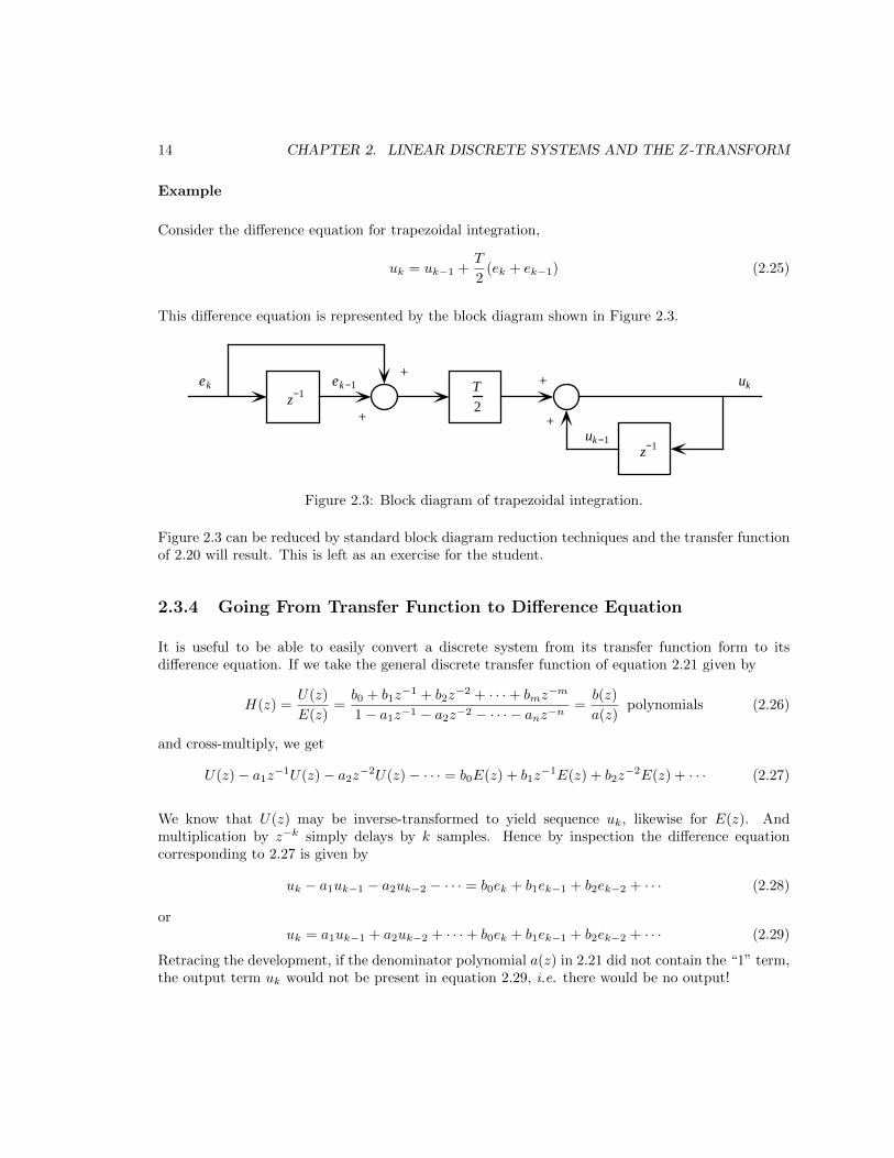
Consider the difference equation for trapezoidal integration,
uk = uk−1 +T
2(ek + ek−1) (2.25)
This difference equation is represented by the block diagram shown in Figure 2.3.
z−1
z−1
T
2
ek ek −1
+
++
+
uk
uk −1
Figure 2.3: Block diagram of trapezoidal integration.
Figure 2.3 can be reduced by standard block diagram reduction techniques and the transfer functionof 2.20 will result. This is left as an exercise for the student.
2.3.4 Going From Transfer Function to Difference Equation
It is useful to be able to easily convert a discrete system from its transfer function form to itsdifference equation. If we take the general discrete transfer function of equation 2.21 given by
H(z) =U(z)
E(z)=b0 + b1z
−1 + b2z−2 + · · ·+ bmz
−m
1− a1z−1 − a2z−2 − · · · − anz−n=b(z)
a(z)polynomials (2.26)
and cross-multiply, we get
U(z)− a1z−1U(z)− a2z
−2U(z)− · · · = b0E(z) + b1z−1E(z) + b2z
−2E(z) + · · · (2.27)
We know that U(z) may be inverse-transformed to yield sequence uk, likewise for E(z). Andmultiplication by z−k simply delays by k samples. Hence by inspection the difference equationcorresponding to 2.27 is given by
uk − a1uk−1 − a2uk−2 − · · · = b0ek + b1ek−1 + b2ek−2 + · · · (2.28)
oruk = a1uk−1 + a2uk−2 + · · ·+ b0ek + b1ek−1 + b2ek−2 + · · · (2.29)
Retracing the development, if the denominator polynomial a(z) in 2.21 did not contain the “1” term,the output term uk would not be present in equation 2.29, i.e. there would be no output!
2.3. THE Z-TRANSFORM AND THE DISCRETE TRANSFER FUNCTION 15
2.3.5 Relation of the Transfer Function to the Unit Pulse Response
Recall that in continuous systems the transfer function of a thing is also equal to the Laplacetransform of the thing’s unit impulse response (easily shown. . . it might be good to verify it). Asimilar relationship holds for discrete systems. Consider a system with transfer function
H(z) =U(z)
E(z)
Let input ek be a unit pulse, i.e.
ek = 1 k = 0
= 0 k 6= 0 (2.30)
= δk (unit discrete pulse at sample zero)
The z-transform of the unit pulse is given by
E(z) =
∞∑k=0
ekz−k = e0z
0 = 1 (2.31)
hence U(z) = H(z), and the discrete transfer function H(z) is the z-transform of the system’s unitpulse response.
Example
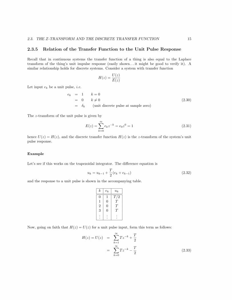
Let’s see if this works on the trapezoidal integrator. The difference equation is
uk = uk−1 +T
2(ek + ek−1) (2.32)
and the response to a unit pulse is shown in the accompanying table.
k ek uk
0 1 T/21 0 T2 0 T3 0 T...
......
Now, going on faith that H(z) = U(z) for a unit pulse input, form this term as follows:
H(z) = U(z) =
∞∑k=1
Tz−k +T
2
=
∞∑k=0
Tz−k − T
2(2.33)
16 CHAPTER 2. LINEAR DISCRETE SYSTEMS AND THE Z-TRANSFORM
To reduce the first term on the right of the “=” sign in 2.33 one must use the expression for thesum of a geometric series. This sum is very useful in expressing z-transforms in closed form.
The sum of a geometric series is given by
∞∑k=0
ark =a
1− r(2.34)
Using equation 2.34 to reduce 2.33 (the “r” term will be z−1) we obtain
H(z) = U(z) =T
1− z−1− T
2=
2T − T (1− z−1)
2(1− z−1)
=T + Tz−1
2(1− z−1)=T
2
1 + z−1
1− z−1=T
2
z + 1
z − 1(2.35)
which agrees with the transfer function of equation 2.20.
2.4 Dynamic Response of Discrete Systems
In this section we will examine the dynamic response of discrete systems and begin to associatez-plane pole and zero location with corresponding response. As a designer, it is important to havea good “feel” for the correlation between z-plane pole and zero location and system response. Wehave already seen the most basic correlation, that of stability. If any poles of the discrete transferfunction are outside the unit circle, the system is unstable.
Indeed, one can use the “brute force” technique, given by
1. Obtain the transfer function H(z) of the system.
2. Look up the z-transform of the input E(z) (a table of z transforms will appear at the end ofthis chapter)
3. Form output U(z) = H(z)E(z)
4. Inverse transform U(z) to get uk.
This can be an involved process, especially inverse transforming. So it is worthwhile to develop agood correlation between pole and zero location and dynamic response. Presumably you have someknowledge of this correlation for continuous systems in the s-plane. . . if not, it would a good idea toreview that now.
Our approach here will be to take three basic discrete functions and examine both their z-transforms(pole locations) and their discrete-domain character. These discrete functions will be

2.4. DYNAMIC RESPONSE OF DISCRETE SYSTEMS 17
1. Unit step.
2. Exponential.
3. Damped sinusoid.
In the three sections to follow, a numerical subscript will be used to indicate these functions, likee1(k), e2(k), and e3(k).
2.4.1 Unit step
The unit step function is given by e1(k) = 1, k ≥ 0, with z-transform
E1(z) =
∞∑k=0
z−k =1
1− z−1=
z
z − 1. (2.36)
The unit step has a pole at z = 1 and a zero at z = 0. A sketch of the pole and zero locations forthe unit step and the corresponding discrete behavior are shown in Figure 2.4.
0 1 2 3 4 50
0.2
0.4
0.6
0.8
1
k
Re
Im
Figure 2.4: Unit step pole/zero locations and response.
2.4.2 Exponential
The discrete exponential function is given by e2(k) = rk, k ≥ 0. The z-transform of this function is
E2(z) =
∞∑k=0
rkz−k =
∞∑k=0
(rz−1
)k=
1
1− rz−1=
z
z − r(2.37)
which has a single real pole at z = r, plus a zero at z = 0. There are a couple of observations aboutthe behavior of the exponential function.

18 CHAPTER 2. LINEAR DISCRETE SYSTEMS AND THE Z-TRANSFORM
• Since the exponential function is e2(k) = rk, if |r| > 1 the response will grow. This correspondsto a pole outside the unit circle. If this were the pulse response of a discrete system the systemwould be unstable. (We saw this in Section 2.2.1).
• If −1 < r < 0, the pole is on the negative real axis (but within the unit circle) the responsewill alternate signs. This form is unique to discrete systems and has no counterpart in thecontinuous domain, as we will see later.
Three examples of pole and zero locations for the exponential function and the corresponding discretebehavior are shown in Figure 2.5.
0 1 2 3 4 50
0.5
1
1.5
k
0 1 2 3 4 50
0.5
1
1.5
k
0 1 2 3 4 5
-0.5
0
0.5
1
1.5
k
Re
Re
Re
Im
Im
Im
Figure 2.5: Exponential pole/zero locations and response.
2.4.3 Damped Sinusoid
The discrete damped sinusoid is given by e3(k) = rk cos(kθ), k ≥ 0. Using an Euler expansion of thecosine, we obtain
e3(k) = rk(ejkθ + e−jkθ
2
)(2.38)
2.4. DYNAMIC RESPONSE OF DISCRETE SYSTEMS 19
Since the z-transform is linear, we can treat each term of equation 2.38 separately, then add thez-transform of both terms at the end. Consider the first term (denominator 2 factored out):
e4(k) = rkejkθ. (2.39)
The z-transform of this discrete function is
E4(z) =
∞∑k=0
rkejkθz−k =
∞∑k=0
(rejθz−1
)k=
1
1− rejθz−1
=z
z − rejθ(2.40)
This function has a single complex pole at z = rejθ. Note that this function will grow if |r| > 1 andwill decay if |r| < 1. Now for the second term in 2.38, it can be shown that
Z e5(k) = Zrke−jkθ
= E5(z) =
z
z − re−jθ, (2.41)
and adding both expressions yields
E3(z) =
(E4(z) + E5(z)
2
)=
z(z − r cos θ)
z2 − 2r cos θz + r2(2.42)
The poles of E3(z) are complex conjugates, and are
z = re±jθ
= r cos θ ± jr sin θ (2.43)
The zeros are real, at 0, r cos θ and are in line with the poles.
Example
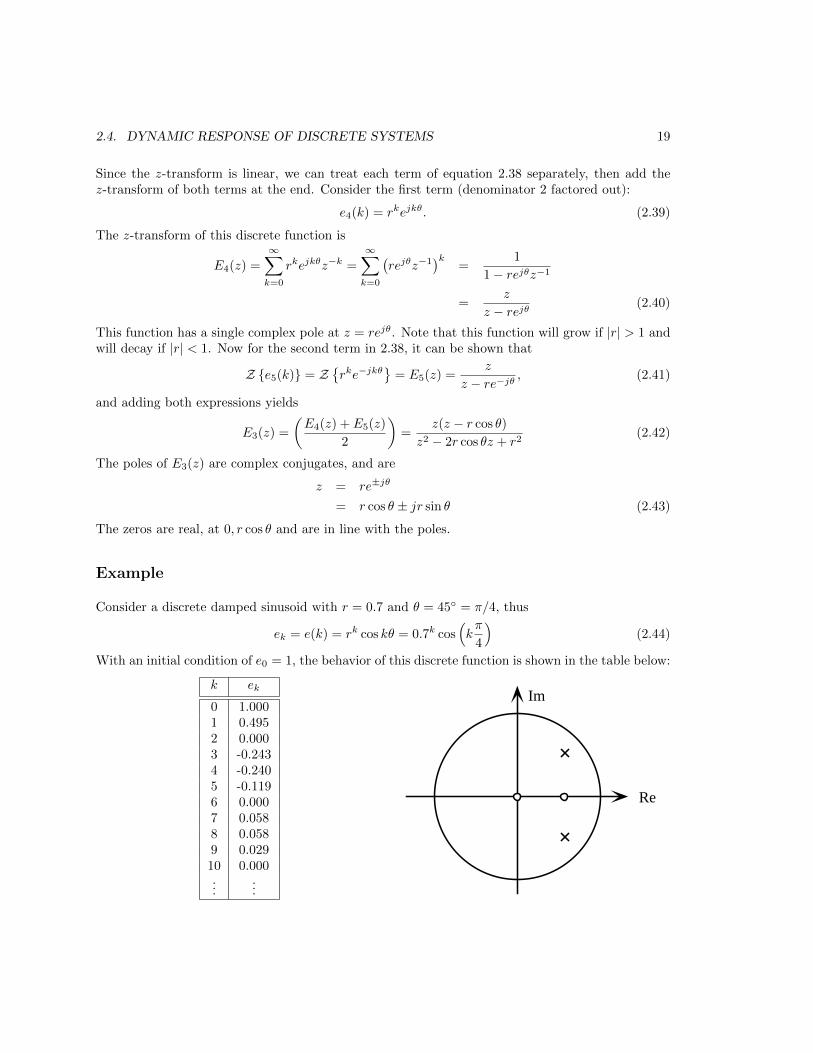
Consider a discrete damped sinusoid with r = 0.7 and θ = 45 = π/4, thus
ek = e(k) = rk cos kθ = 0.7k cos(kπ
4
)(2.44)
With an initial condition of e0 = 1, the behavior of this discrete function is shown in the table below:
k ek
0 1.0001 0.4952 0.0003 -0.2434 -0.2405 -0.1196 0.0007 0.0588 0.0589 0.02910 0.000...
...
Re
Im
20 CHAPTER 2. LINEAR DISCRETE SYSTEMS AND THE Z-TRANSFORM
0 2 4 6 8 10-0.4
-0.2
0
0.2
0.4
0.6
0.8
1
Sample Index k
Dam
ped
Sin
usoi
d e(
k)
Figure 2.6: Discrete damped sinusoidal response.
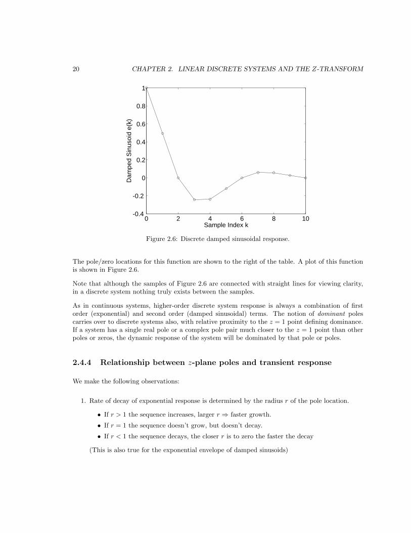
The pole/zero locations for this function are shown to the right of the table. A plot of this functionis shown in Figure 2.6.
Note that although the samples of Figure 2.6 are connected with straight lines for viewing clarity,in a discrete system nothing truly exists between the samples.
As in continuous systems, higher-order discrete system response is always a combination of firstorder (exponential) and second order (damped sinusoidal) terms. The notion of dominant polescarries over to discrete systems also, with relative proximity to the z = 1 point defining dominance.If a system has a single real pole or a complex pole pair much closer to the z = 1 point than otherpoles or zeros, the dynamic response of the system will be dominated by that pole or poles.
2.4.4 Relationship between z-plane poles and transient response
We make the following observations:
1. Rate of decay of exponential response is determined by the radius r of the pole location.
• If r > 1 the sequence increases, larger r ⇒ faster growth.
• If r = 1 the sequence doesn’t grow, but doesn’t decay.
• If r < 1 the sequence decays, the closer r is to zero the faster the decay
(This is also true for the exponential envelope of damped sinusoids)

2.5. CORRESPONDENCE BETWEEN DISCRETE AND CONTINUOUS SIGNALS 21
2. The oscillation speed (number of samples/cycle) of complex poles is determined by their angleθ. Given
ek = cos kθ (2.45)
let N be the number of samples per oscillation period, hence
cos kθ = cos [(k +N)θ] = cos(kθ +Nθ). (2.46)
Since N is defined to be the period, we must have
Nθ = 2π (2.47)
hence the period N is given by
N =2π
θrad=
360
θdeg(2.48)
Example
In the previous example, we had a damped sinusoidal response. The period of this response is givenby
N =360
θdeg=
360
45= 8 samples (2.49)
Examination of the response in both the table and figure verifies this period.
2.4.5 Effect of Zeros on Dynamic Response
In continuous transfer functions, zeros represent derivatives of the input which are transferred tothe output, thus speeding up response and increasing overshoot.
The same is true of discrete transfer functions, with the effect of a z-plane zero greater when it isnear z = 1, and its effect decreasing as it is far from z = 1. Note that a zero at z = 0 represents aunit advance, just as a pole at z = 0 is a unit delay.
2.5 Correspondence between Discrete and Continuous Sig-nals
So far in this chapter we have considered discrete systems only. It is time to make a connectionbetween discrete and continuous systems, and in the process to develop a very useful mathematicallink between the z domain and the s domain.
Consider discrete variable y(k) (yk could be used), where we now say that this y(k) was obtainedby sampling continuous signal y(t) at sample period T . We shall use a damped sinusoid for thisdevelopment.
22 CHAPTER 2. LINEAR DISCRETE SYSTEMS AND THE Z-TRANSFORM
The continuous signaly(t) = e−at cos bt (2.50)
has Laplace transform
Y (s) =s+ a
(s+ a)2 + b2(2.51)
and the poles of Y (s) are ats = −a± jb (2.52)
Now, if we sample e−at cos bt at sample period T , at sample times of t = kT , we will get discretesignal
y(kT ) = e−akT cos bkT (2.53)
which is of the form rk cos kθ, where r and θ given by
r = e−aT , θ = bT (2.54)
We saw from Equation 2.43 that a discrete damped sinusoid has z-plane poles at
z = re±jθ (2.55)
which here becomesz = re±jθ = e−aT e±jbT = e(−a±jb)T (2.56)
Compare the s-plane pole locations of 2.52 and the z-plane poles of 2.56. The pole locations arerelated by
z = esT (2.57)
This is a general relationship between poles of continuous signals and their discrete counterparts,and can be expressed in terms of pole locations:
Poles in the s-plane and z-plane are related by z = esT . Note that this is not true of zeros.
This mapping between the s and the z plane is very useful in design.
Example
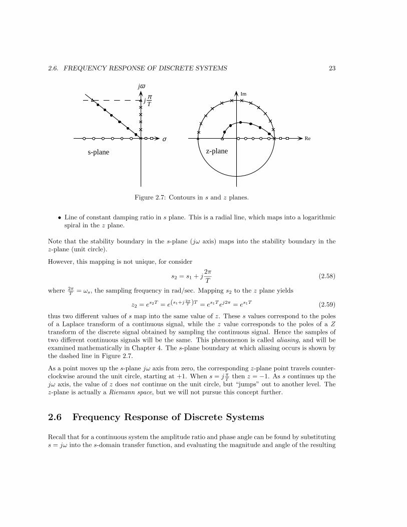
Let’s examine the mapping between some contours in the s plane and z plane, with reference toFigure 2.7.
• s-plane origin. This maps into z = esT = 1, on the unit circle.
• s-plane real axis from 0→ −∞. Using z = esT this maps into the z real axis from +1→ 0.
• s-plane jω axis. This maps into z = ejωT , which is the unit circle itself.
2.6. FREQUENCY RESPONSE OF DISCRETE SYSTEMS 23
jπT
σ
jω
Re
Im
s-plane z-plane
Figure 2.7: Contours in s and z planes.
• Line of constant damping ratio in s plane. This is a radial line, which maps into a logarithmicspiral in the z plane.
Note that the stability boundary in the s-plane (jω axis) maps into the stability boundary in thez-plane (unit circle).
However, this mapping is not unique, for consider
s2 = s1 + j2π
T(2.58)
where 2πT = ωs, the sampling frequency in rad/sec. Mapping s2 to the z plane yields
z2 = es2T = e(s1+j 2πT )T = es1T ej2π = es1T (2.59)
thus two different values of s map into the same value of z. These s values correspond to the polesof a Laplace transform of a continuous signal, while the z value corresponds to the poles of a Ztransform of the discrete signal obtained by sampling the continuous signal. Hence the samples oftwo different continuous signals will be the same. This phenomenon is called aliasing, and will beexamined mathematically in Chapter 4. The s-plane boundary at which aliasing occurs is shown bythe dashed line in Figure 2.7.
As a point moves up the s-plane jω axis from zero, the corresponding z-plane point travels counter-clockwise around the unit circle, starting at +1. When s = j πT then z = −1. As s continues up thejω axis, the value of z does not continue on the unit circle, but “jumps” out to another level. Thez-plane is actually a Riemann space, but we will not pursue this concept further.
2.6 Frequency Response of Discrete Systems
Recall that for a continuous system the amplitude ratio and phase angle can be found by substitutings = jω into the s-domain transfer function, and evaluating the magnitude and angle of the resulting

24 CHAPTER 2. LINEAR DISCRETE SYSTEMS AND THE Z-TRANSFORM
expression.
A similar technique works for discrete systems, and will be given without proof. Consider a discretesystem with input uk, output yk, and discrete transfer function
H(z) =Y (z)
U(z)(2.60)
If the input is a sinusoid at frequency ωo
uk = Uo cos(ωokT ) (2.61)
the steady-state output will also be sinusoidal, of the form
yk = Yo cos(ωokT + φ) (2.62)
where the amplitude ratio Yo/Uo and phase angle φ are given by
YoUo
= |H(z)|z=ejωoT (2.63)
andφ = 6 H(z)|z=ejωoT (2.64)
There will be numerous calculations of the frequency response of discrete systems in Chapter 3, sowe will defer examples until that point.
2.7 Z-Transform Properties
In this section are a few of the more useful properties of the z-transform.
1. Linearity. The z-transform is linear, i.e.
Z αf1(kT ) + βf2(kT ) = αF1(z) + βF2(z)
2. Time Shift. We have seen this with the unit delay and advance:
Z f(k + n) = znF (z)
3. Final Value Theorem. If (z − 1)F (z) has all poles inside the unit circle, and has no poles onthe unit circle except possibly one pole at z = 1 (i.e.. not unstable), then the terms in thesequence f(k) due to poles inside the unit circle→ 0 as k →∞. The only value left as k →∞will be that due to the pole at z = 1, this value is the final value, and may be found as theresidue of the 1
z−1 term in a partial fraction expansion of F (z).
limk→∞
f(k) = (z − 1) F (z)|z=1 (2.65)
This is called the Final Value Theorem, and is very useful. The final value theorem may beused to find the DC gain of a discrete transfer function.

2.7. Z-TRANSFORM PROPERTIES 25
DC gain of transfer function
Given
H(z) =Y (z)
U(z)(2.66)
let input uk be a step of magnitude u∞, with z-transform
U(z) =u∞z
z − 1(2.67)
The output is given by
Y (z) = H(z)U(z) = H(z)u∞z
z − 1(2.68)
The final value of output sequence yk can be found using the final value theorem, and is
limk→∞
= y∞ = (z − 1) Y (z)|z=1 = (z − 1) H(z)u∞z
z − 1
∣∣∣∣z=1
= u∞H(1) (2.69)
Hence the DC gain of the transfer function H(z) is
y∞u∞
= H(1) (2.70)
Note that to apply the final value theorem to a discrete variable, that variable must have afinal value. Responses that are unbounded will yield arithmetic results which are not valid.
When finding the DC gain of a transfer function, all poles of the transfer function must beinside the unit circle.
Example
Consider the discrete transfer function given by
H(z) =Y (z)
U(z)=
z + 1
z2 − 0.5z + 0.5=
z + 1
z − 0.25± j0.66(2.71)
Note that it is necessary to find the pole locations of this transfer function to make sure it is stable(all poles inside unit circle). The DC gain is given by
H(1) =1 + 1
1− 0.5 + 0.5= 2 (2.72)
Thus if this discrete system were given an input that eventually reached a constant value, the outputwould eventually reach twice that value.
NOTE: If the denominator polynomial above were z2 − 0.5z + 2, the DC gain would evaluate toH(1) = 0.8, but that is meaningless since the system is unstable.

26 CHAPTER 2. LINEAR DISCRETE SYSTEMS AND THE Z-TRANSFORM
2.7.1 Inverse Transforming
Just as in continuous linear dynamic system analysis, given a z-transform F (z) it is of fundamentalimportance to obtain the corresponding discrete sequence f(k). There are several methods.
Synthetic division
Given the definition of the z-transform for F (z), expressed as a ratio of polynomials in z−1:
F (z) =∞
limk=0
f(k)z−k =b(z−1)
a(z−1)(2.73)
The discrete sequence fk may be recovered from F (z) by direct synthetic division. The coefficientof z−k in the quotient will be the kth sample.
Example
An s-plane pole at s = −2 has time constant τ = 0.5 sec. Let sample period T = 0.1 sec, corre-sponding to sampling frequency fs = 10 Hz. (Note that T is one-fifth τ . . . fast enough to “catch”the dynamic response.) The s-plane pole corresponds to a z-plane pole at
z = esT = e−0.2 = 0.8187 (2.74)
Define a discrete transfer function with this pole and a DC gain of 1, thus
H(z) =0.1813
z − 0.8187=Y (z)
U(z)(2.75)
Let the input U(z) be a unit step, z/(z − 1), thus the response Y (z) is
Y (z) =0.1813z
(z − 0.8187)(z − 1)=
0.1813z
z2 − 1.8187z + 0.8187=
0.1813z−1
1− 1.8187z−1 + 0.8187z−2(2.76)
The sequence y(k) can be obtained by the synthetic division of the polynomials in Y (z) above. Asmentioned above, the coefficient of z0 in the quotient will be the 0th sample, the coefficient of z−1
will be the 1st sample, the coefficient of z−2 will be the 2nd sample, and so on. This method istedious for manual computation, but lends itself well to construction of a numerical algorithm forinversion by computer.
Difference equation
In this method we convert the discrete transfer function to a difference equation (see Section 2.3.4),then simply evaluate the equation as presented at the beginning of Section 2.2. We will use thismethod on the system of the previous example.
2.7. Z-TRANSFORM PROPERTIES 27
Example
Again take discrete transfer function
H(z) =0.1813
z − 0.8187=Y (z)
U(z)(2.77)
with corresponding transform equation
Y (z)− 0.8187z−1Y (z) = 0.1813z−1U(z) (2.78)
or
yk − 0.8187yk−1 = 0.1813uk−1 (2.79)
which yields
yk = 0.8187yk−1 + 0.1813uk−1 (2.80)
This difference equation can be evaluated for any input. For a unit step input one can generate thefollowing table:
k uk yk
0 1 01 1 0.18132 1 0.32973 1 0.45134 1 0.55075 1 0.63226 1 0.69897 1 0.7535...
......
∞ 1 1.0000
Note that the response yk reaches 63% of the final value at k = 5, or t = 0.5 sec, the time constantof the original continuous pole. This method is acceptable for hand calculation for a few samples,but tedious for many samples.
Table lookup
Just as with the Laplace transform, the discrete sequence f(k) corresponding to F (z) may be foundby table lookup. It is often complicated by the need to do partial fraction expansion. Again, considerthe same example,
Y (z) =0.1813z
(z − 0.8187)(z − 1)=
0.1813z
z2 − 1.8187z + 0.8187(2.81)
28 CHAPTER 2. LINEAR DISCRETE SYSTEMS AND THE Z-TRANSFORM
This Y (z) is not in the table of Section 2.9 (admittedly a small table) so we must expand in partialfractions
Y (z) =0.1813z
(z − 0.8187)(z − 1)=
0.1813z
z2 − 1.8187z + 0.8187=
1
z − 1− 0.8187
z − 0.8187(2.82)
Transform numbers 1 and 3 from Section 2.9 come close to fitting these terms, but they must beexpressed as
Y (z) = (z−1)z
z − 1+ (0.8187z−1)
z
z − 0.8187. (2.83)
Transform pairs 1 and 3 are then applicable, and since z−1 is the unit delay, we can write
yk = 1(k − 1) + 0.8187k (2.84)
which should yield the same result as the previous two methods.
MATLAB simulation
This is by far the most useful method, providing that the problem is numerical!. Consider theprevious transfer function,
H(z) =0.1813
z − 0.8187(2.85)
An easy way to “inverse transform” Y (z) using MATLAB is to employ the dlsim(num,den,u) func-tion (discrete linear simulation), where num is the numerator polynomial of the transfer function(coefficients of decreasing powers of z), den is the denominator polynomial, and u is the input. TheMATLAB script below does this for a unit step:
>>u = ones(size(0:10)); % Define input to be "1" from samples 0 to 10
>>num = [0 0.1813]; % Numerator coefficients of z
>>den = [1 -0.8187]; % Denominator coefficients of z
>>y = dlsim(num,den,u) % Do the simulation, displaying resulting samples
y =
0
0.1813
0.3297
0.4513
0.5507
0.6322
0.6989
0.7535
0.7982
0.8348
0.8647
>>plot(0:10,y,’o’,0:10,y); % Plot samples as "o" connected by lines
2.7. Z-TRANSFORM PROPERTIES 29
0 2 4 6 8 100
0.1
0.2
0.3
0.4
0.5
0.6
0.7
0.8
0.9
Sample Index k
Res
pons
e y(
k)
Figure 2.8: Step response of discrete system.
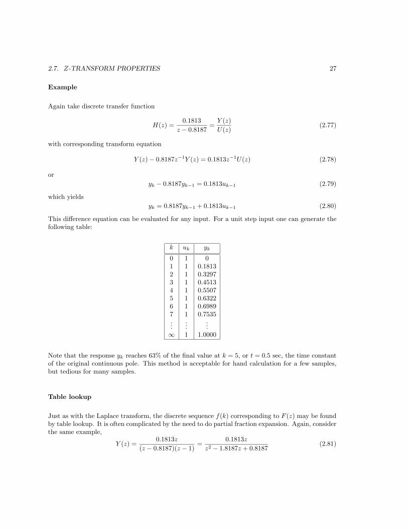
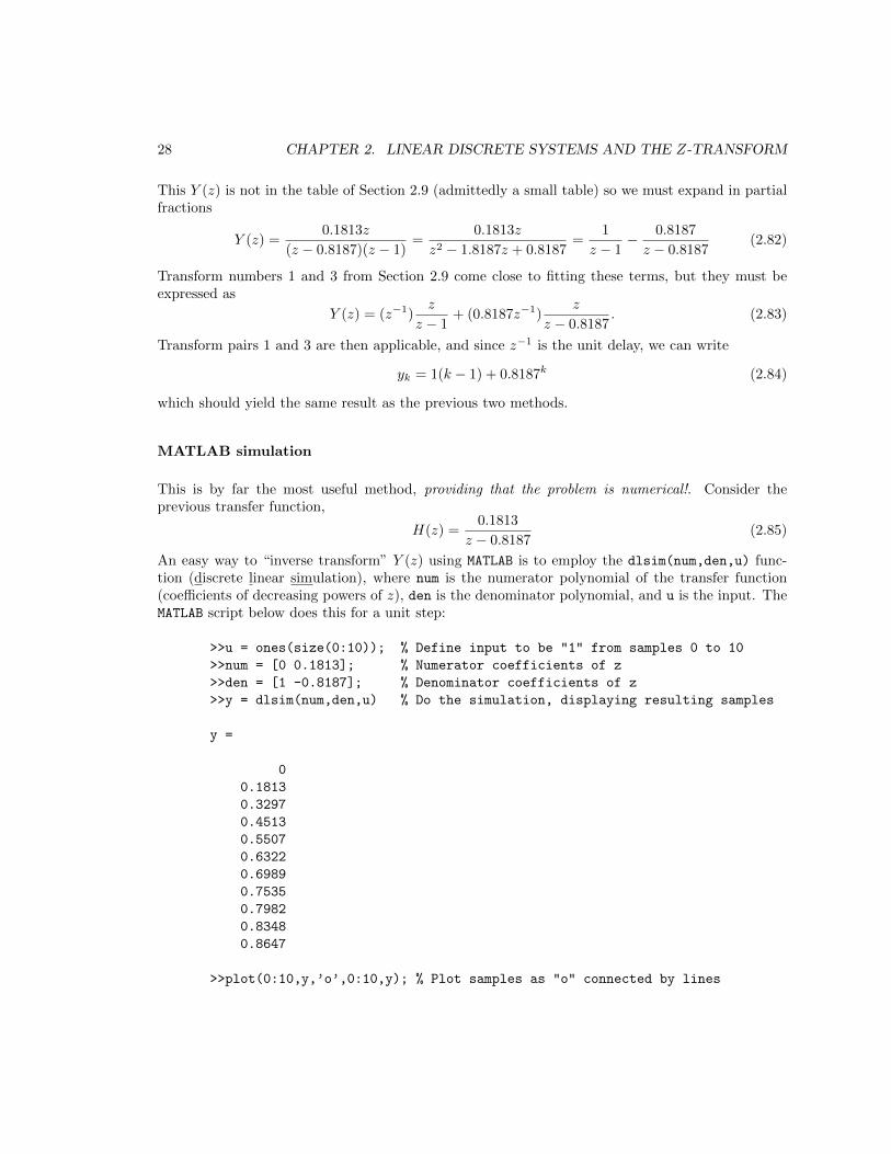
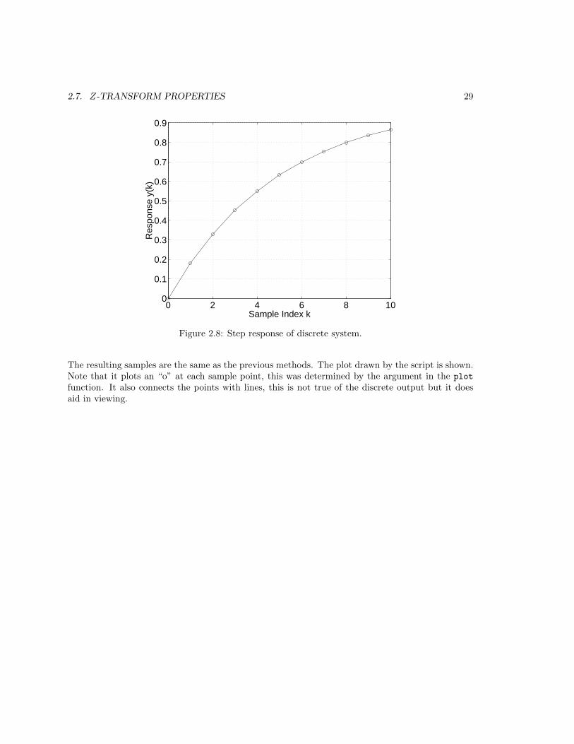
The resulting samples are the same as the previous methods. The plot drawn by the script is shown.Note that it plots an “o” at each sample point, this was determined by the argument in the plot
function. It also connects the points with lines, this is not true of the discrete output but it doesaid in viewing.

30 CHAPTER 2. LINEAR DISCRETE SYSTEMS AND THE Z-TRANSFORM
Other MATLAB Functions (DSTEP, DDCGAIN)
Although dlsim is more general the DSTEP(NUM,DEN) function produces the unit step responsedirectly. I usually use it with a returned argument as follows:
>> y = dstep(num,den); % Obtain unit step response
>> plot(...); % Plot as desired...
The DC Gain K of a discrete transfer function may be found using ddcgain if the system is describedusing explicit num and den, or using dcgain if the system is described using an “LTI” model (seeSection 2.8 below).
>> K = DDCGAIN(NUM,DEN); % NUM and DEN are vectors w/polynomial coefficients
>> K = DCGAIN(SYS); % SYS is a discrete transfer function in LTI format
2.8 A Word about LTI Systems and MATLAB functions
There has been a fundamental change in MATLAB since I first wrote these notes in 1998. This hasdo to with the “LTI System” and the notion of “overloaded functions.”
2.8.1 LTI Systems
An LTI System is MATLAB’s representation of any dynamic system (either continuous- or discrete-time, modeled using either transfer-function or state-variable formulation), and can be created inseveral ways:
• TF—using numerator and denominator of transfer function (either continuous- or discrete-time)
• ZPK—using zeros, poles, and gain of a transfer function (either...)
• SS—using state-space formulations (Chapters 6-8 of these notes)
Sometimes it is advantageous to cast systems into LTI format (certain MATLAB functions requirethat)—otherwise it may be useful to have them in numerator/denominator, zero/pole/gain, or ex-plicit state-space format. You will see all representations at various times in these notes. LTIsystems are created using the three MATLAB functions listed above (TF,ZPK,SS)—type help tf,help zpk,etc in MATLAB to see more discussion.
Note that if a sample period T is used when creating an LTI model, then that model is automaticallymade a discrete-time model. This is very important.

2.8. A WORD ABOUT LTI SYSTEMS AND MATLAB FUNCTIONS 31
2.8.2 Overloaded Functions
The concept of overloading has its origin in object-oriented programming, and means that the samefunction will operate differently on different objects. For MATLAB, this means that the samefunction can be used on different LTI systems, e.g. continuous-time and discrete-time.
As an example, consider the MATLAB step function, which produces the unit step response of adynamic system. An excerpt from the MATLAB “help” resource indicates:
>> help step
STEP Step response of LTI models.
STEP(SYS) plots the step response of the LTI model SYS (created
with either TF, ZPK, or SS). For multi-input models, independent
step commands are applied to each input channel. The time range
and number of points are chosen automatically.
...
Note that there is no mention of whether “sys” is continuous or discrete—the step function willhandle them both! When you create the LTI object you specify its nature; this is used by step tocompute the response correctly.
Consider the following two transfer functions G(s) and G(z):
G(s) =1
s+ 1G(z) =
0.1813
z − 0.8187, T = 0.2
Now create LTI systems Gc and Gd for each transfer function:
>> Gc = tf([0 1],[1 1]) % Enter numerator and denominator polynomials
Transfer function:
1
-----
s + 1
>> Gd = tf([0 0.1813],[1 -0.8187],0.2) % Note sample period T = 0.2
Transfer function:
0.1813
----------
z - 0.8187
Sampling time: 0.2
By appending the “0.2” to the creation of Gd we obtained a discrete-time LTI model.
We can apply the step function to either model:

32 CHAPTER 2. LINEAR DISCRETE SYSTEMS AND THE Z-TRANSFORM
>> step(Gc);
>> step(Gd);
Try it! Both commands will produce plots of the response; the discrete-time system will yield a“stairstep” plot (sometimes appropriate, sometimes not).
Many MATLAB functions are “overloaded” and apply to both types of systems. I’m slowly revisingthese notes, and I’ll try to show examples during class.
2.9 Table of Z-Transforms
The short table below lists some z-transforms. F(s) is the Laplace transform of f(t) and F (z) isthe z-transform of f(kT ).
Number F(s) f(kT ) F (z)
1 1s 1(kT ) z
z−1
2 1s2 kT Tz
(z−1)2
3 1s+a e−akT z
z−e−aT
4 1(s+a)2 kTe−akT Tze−aT
(z−e−aT )2
5 as(s+a) 1− e−akT z(1−e−aT )
(z−1)(z−e−aT )
6 as2+a2 sin akT z sin aT
z2−(2 cos aT )z+1
7 ss2+a2 cos akT z(z−cos aT )
z2−(2 cos aT )z+1
8 s+a(s+a)2+b2 e−akT cos bkT z(z−e−aT cos bT )
z2−2e−aT (cos bT )z+e−2aT
9 b(s+a)2+b2 e−akT sin bkT ze−aT sin bT
z2−2e−aT (cos bT )z+e−2aT
10 a2+b2
s((s+a)2+b2) 1− e−akT(cos bkT + a
b sin bkT) z(Az+B)
(z−1)(z2−2e−aT (cos bT )z+e−2aT )
A = 1− e−aT cos bT − ab e−aT sin bT
B = e−2aT + ab e−aT sin bT − e−aT cos bT
2.9. TABLE OF Z-TRANSFORMS 33
Homework Problems
Problem 1.
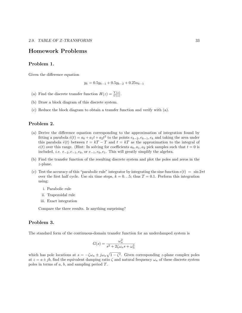
Given the difference equation
yk = 0.5yk−1 + 0.5yk−2 + 0.25uk−1
(a) Find the discrete transfer function H(z) = Y (z)U(z) .
(b) Draw a block diagram of this discrete system.
(c) Reduce the block diagram to obtain a transfer function and verify with (a).
Problem 2.
(a) Derive the difference equation corresponding to the approximation of integration found byfitting a parabola e(t) = a0 + a1t+ a2t
2 to the points ek−2, ek−1, ek and taking the area underthis parabola e(t) between t = kT − T and t = kT as the approximation to the integral ofe(t) over this range. (Hint: In solving for coefficients a0, a1, a2 pick samples such that t = 0 isincluded, i.e. e−2, e−1, e0, or e−1, e0, e1. This will greatly simplify the algebra.
(b) Find the transfer function of the resulting discrete system and plot the poles and zeros in thez-plane.
(c) Test the accuracy of this “parabolic rule” integrator by integrating the sine function e(t) = sin 2πtover the first half cycle. Use six time steps, k = 0. . .5; thus T = 0.1. Perform this integrationusing:
i. Parabolic rule
ii. Trapezoidal rule
iii. Exact integration
Compare the three results. Is anything surprising?
Problem 3.
The standard form of the continuous-domain transfer function for an underdamped system is
G(s) =ω2n
s2 + 2ζωns+ ω2n
which has pole locations at s = −ζωn ± jωn√
1− ζ2. Given corresponding z-plane complex polesat z = a± jb, find the equivalent damping ratio ζ and natural frequency ωn of these discrete systempoles in terms of a, b, and sampling period T .

34 CHAPTER 2. LINEAR DISCRETE SYSTEMS AND THE Z-TRANSFORM
Problem 4.
For the discrete transfer function G(z) below:
G(z) =1
z2 − 0.5z + 0.5
(a) Find and plot the unit pulse response.
(b) Find and plot the unit step response. Also verify the DC gain using the method of Section 2.7.
(c) Find and plot the response to a sine input of 0.5 Hz. Assume a sample period T = 0.2 seconds.Verify the amplitude ratio and phase shift with that computed analytically using the frequencyresponse method of Section 2.6. (Hint: You should use MATLAB to do this one, there are toomany samples to compute by hand, since you must simulate it until the response reaches steadystate).

Chapter 3
Discrete Simulation of ContinuousSystems
Finding a discrete system which simulates the behavior of a given continuous system is important indiscrete-domain control system design, since the (continuous) plant’s response to a discretized inputmust be known before a controller can be designed for that plant.
However, the study of discrete simulations of continuous systems is important in its own right,because we often have a known H(s) which we wish to realize using a computer, hence we mustfind a discrete system H(z) which yields the same behavior. All dynamic systems H(s) may beconsidered filters, hence the subject matter of this chapter is sometimes called digital filtering.
3.1 Chapter Overview
Linear filters may be described by their frequency behavior, i.e. their amplitude and phase charac-teristics vs frequency. In this chapter we will often judge the accuracy of our discrete simulations bycomparing their frequency characteristics to the frequency characteristics of the original continuoussystem. Some types of filters are
• Radio receiver filter—bandpass
• Power line noise filter—bandstop
• Audio applications—equalizer
• Control system filters—compensators
These are all fundamentally similar, they have certain amplitude ratio and phase shift vs frequency.Continuous filter design is an established area. We will assume the continuous filter is known, andpose the problem
35
36 CHAPTER 3. DISCRETE SIMULATION OF CONTINUOUS SYSTEMS
Given H(s), what H(z) will have approximately the same characteristics?
We will look at two approaches. . .
1. Numerical Integration.
2. Pole-Zero Mapping.
3.2 Discrete Simulation using Numerical Integration
You have probably used numerical integration to solve differential equations. We are doing the samething here, except we are going to use the result in real time. By the way, trying to define what“real-time” means has resulted in endless arguments. For the purposes of this class, “real time” willmean “keeping up with the hardware.” Controlling a physical process will require sampling at adesired rate. Our digital controller must be able to generate outputs at this rate. Typically, needfor real-time behavior precludes the use of “batch” or multi-user computer operating systems (likeUnix), since they do not guarantee any minimum response or sampling time. One of the figures ofmerit of a real-time operating system (of which there are many, e.g. VxWorks, LynxOS (not Linux!),MATLAB Real-Time Workshop) is its interrupt latency, which defines how fast the computer canrespond to an external event, such as the need of the controlled process for an input. Interruptlatencies of competitive real-time OS’s are well under 10 µsec.
In using numerical integration to obtain a real-time discrete equivalent of a continuous system, wedo the following:
H(s)
⇓Differential Equation
⇓Integrate Numerically
⇓H(z)
Given the need for fast response, we typically use simple numerical integration algorithms. . . youwon’t see any 4th − 5th order Runge-Kutta methods here! The process is best illustrated by anexample:
Example
Given the first-order system
H(s) =U(s)
E(s)=
a
s+ a(3.1)
3.2. DISCRETE SIMULATION USING NUMERICAL INTEGRATION 37
we can cross-multiply to get
sU(s) + aU(s) = aE(s)⇒ u(t) + au(t) = ae(t) (3.2)
henceu(t) = −au(t) + ae(t) (3.3)
We can therefore integrate u to obtain u,
u(t) =
∫ t
0
[−au(τ) + ae(τ)]dτ (3.4)
where the dummy time variable τ is used as the integrand to avoid confusion with time variable t,the upper limit on the integration.
In discrete time, we can express this integral in two parts. . . the integral from t = 0 to the previoussample time t = kT − T , and the integral from t = kT − T to the current sample time t = kT , or
u(kT ) =
∫ kT−T
0
(−au+ ae)dτ +
∫ kT
kT−T(−au+ ae)dτ
= u(kT − T ) + [Area of − au+ ae over kT − T ≤ τ ≤ kT ] (3.5)
This area may be approximated with many numerical rules, we will show four:
• Forward rectangular
• Backward rectangular
• Trapezoidal
• Prewarped trapezoidal
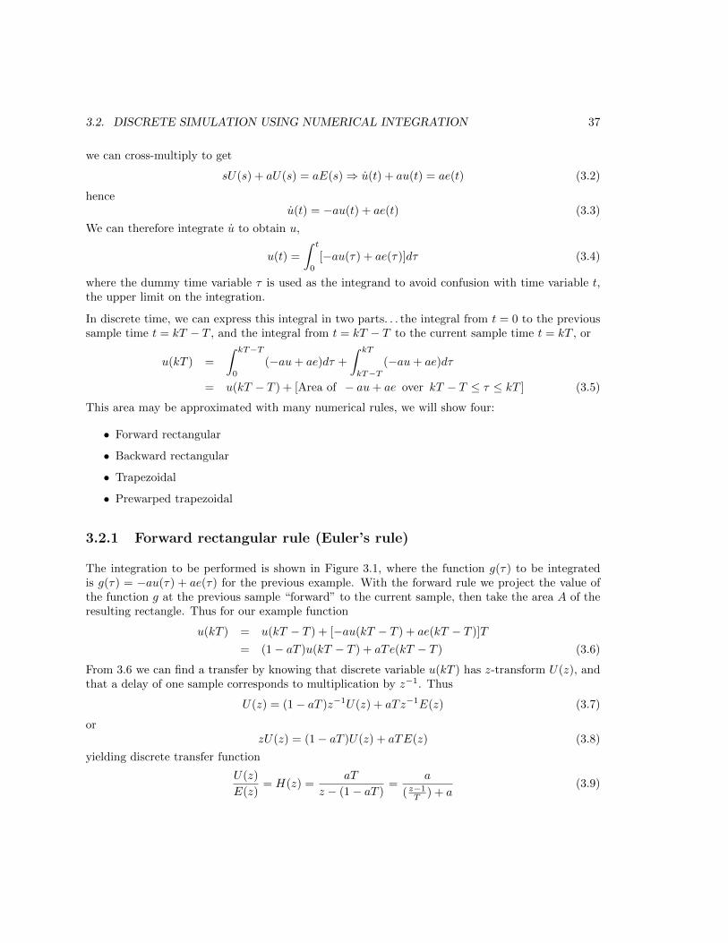
3.2.1 Forward rectangular rule (Euler’s rule)
The integration to be performed is shown in Figure 3.1, where the function g(τ) to be integratedis g(τ) = −au(τ) + ae(τ) for the previous example. With the forward rule we project the value ofthe function g at the previous sample “forward” to the current sample, then take the area A of theresulting rectangle. Thus for our example function
u(kT ) = u(kT − T ) + [−au(kT − T ) + ae(kT − T )]T
= (1− aT )u(kT − T ) + aTe(kT − T ) (3.6)
From 3.6 we can find a transfer by knowing that discrete variable u(kT ) has z-transform U(z), andthat a delay of one sample corresponds to multiplication by z−1. Thus
U(z) = (1− aT )z−1U(z) + aTz−1E(z) (3.7)
orzU(z) = (1− aT )U(z) + aTE(z) (3.8)
yielding discrete transfer function
U(z)
E(z)= H(z) =
aT
z − (1− aT )=
a
( z−1T ) + a
(3.9)

38 CHAPTER 3. DISCRETE SIMULATION OF CONTINUOUS SYSTEMS
g(t)
tkT − T kT
Figure 3.1: Forward integration rule.
3.2.2 Backward rectangular rule
The integration to be performed is shown in Figure 3.2, where the function g(τ) to be integrated isagain g(τ) = −au(τ) + ae(τ). With the backward rule we project the value of the function g at thecurrent sample “back” to the previous sample, then take the area A of the resulting rectangle. Thusfor our example function
u(kT ) = u(kT − T ) + [−au(kT ) + ae(kT )]T
u(kT )(1 + aT ) = u(kT − T ) + aTe(kT ) (3.10)
From (3.10) we can again find a transfer function as in Section 3.2.1. Thus
U(z)(1 + aT ) = z−1U(z) + aTE(z) (3.11)
orU(z)(z + aTz) = U(z) + aTzE(z) (3.12)
thusU(z)(z + aTz − 1) = aTzE(z) (3.13)
yielding discrete transfer function
U(z)
E(z)= H(z) =
aTz
z − 1 + aTz=
a
( z−1Tz ) + a
(3.14)
3.2.3 Trapezoidal rule
This integration rule, sometimes called the Bilinear Transformation or Tustin Approximation, isshown in Figure 3.3, where the function g(τ) to be integrated is still

3.2. DISCRETE SIMULATION USING NUMERICAL INTEGRATION 39
g(t)
tkT − T kT
Figure 3.2: Backward integration rule.
g(τ) = −au(τ) + ae(τ)
With the trapezoidal rule we connect the current sample to the previous sample with a straight line,then take the area A of the resulting trapezoid. This may be thought of as an average of the forwardrectangle and the backward rectangle. For our example function
u(kT ) = u(kT − T ) +T
2[−au(kT − T ) + ae(kT − T )− au(kT ) + ae(kT )] (3.15)
From (3.15) we can again find a transfer function,
U(z) = z−1U(z) +T
2
[−az−1U(z) + az−1E(z)− aU(z) + aE(z)
](3.16)
and after some algebra we obtain discrete transfer function
U(z)
E(z)= H(z) =
aT2 (z + 1)
z − 1 + aT2 (z + 1)=
a(2Tz−1z+1
)+ a
(3.17)
Comparison of the Integration Rules
Comparing the original H(s) =a
s+ awith the three discrete equivalents H(z), an approximation
for s results:
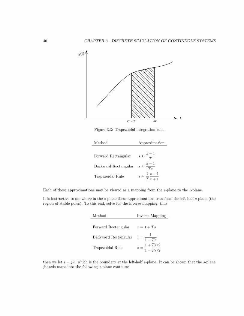
40 CHAPTER 3. DISCRETE SIMULATION OF CONTINUOUS SYSTEMS
g(t)
tkT − T kT
Figure 3.3: Trapezoidal integration rule.
Method Approximation
Forward Rectangular s ≈ z − 1
T
Backward Rectangular s ≈ z − 1
Tz
Trapezoidal Rule s ≈ 2
T
z − 1
z + 1
Each of these approximations may be viewed as a mapping from the s-plane to the z-plane.
It is instructive to see where in the z-plane these approximations transform the left-half s-plane (theregion of stable poles). To this end, solve for the inverse mapping, thus
Method Inverse Mapping
Forward Rectangular z = 1 + Ts
Backward Rectangular z =1
1− Ts
Trapezoidal Rule z =1 + Ts/2
1− Ts/2
then we let s = jω, which is the boundary at the left-half s-plane. It can be shown that the s-planejω axis maps into the following z-plane contours:
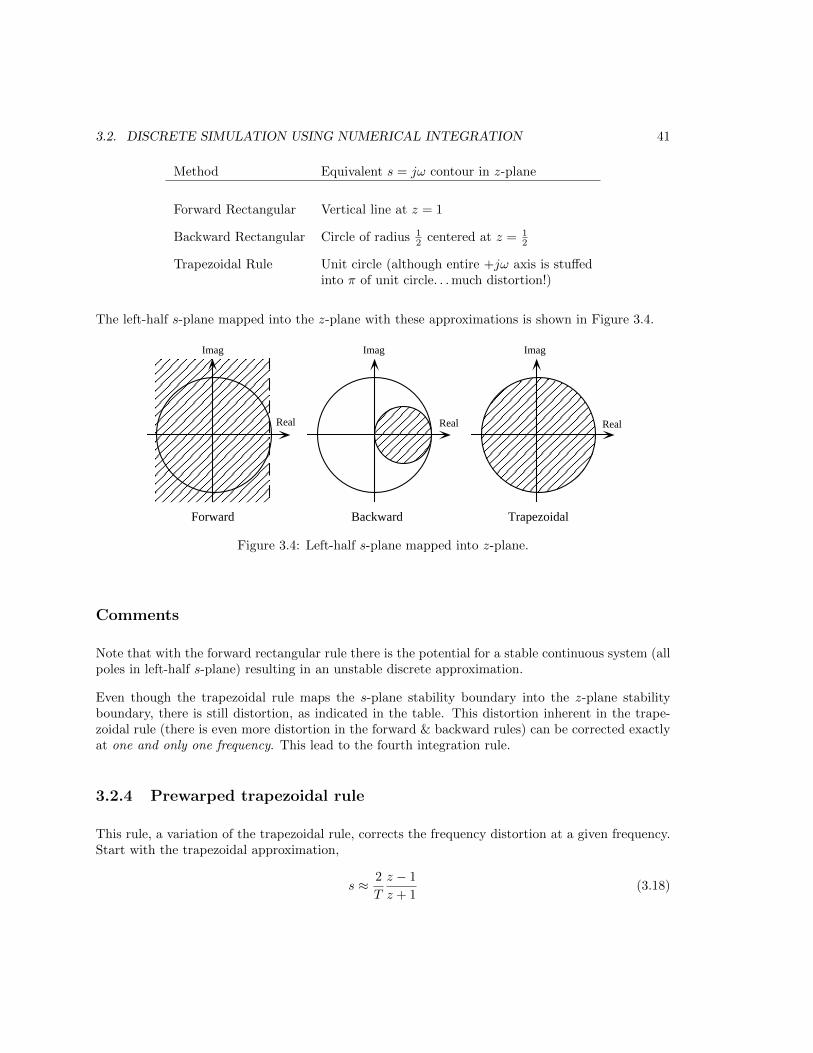
3.2. DISCRETE SIMULATION USING NUMERICAL INTEGRATION 41
Method Equivalent s = jω contour in z-plane
Forward Rectangular Vertical line at z = 1
Backward Rectangular Circle of radius 12 centered at z = 1
2
Trapezoidal Rule Unit circle (although entire +jω axis is stuffedinto π of unit circle. . . much distortion!)
The left-half s-plane mapped into the z-plane with these approximations is shown in Figure 3.4.
Real
Imag Imag Imag
Real Real
Forward Backward Trapezoidal
Figure 3.4: Left-half s-plane mapped into z-plane.
Comments
Note that with the forward rectangular rule there is the potential for a stable continuous system (allpoles in left-half s-plane) resulting in an unstable discrete approximation.
Even though the trapezoidal rule maps the s-plane stability boundary into the z-plane stabilityboundary, there is still distortion, as indicated in the table. This distortion inherent in the trape-zoidal rule (there is even more distortion in the forward & backward rules) can be corrected exactlyat one and only one frequency. This lead to the fourth integration rule.
3.2.4 Prewarped trapezoidal rule
This rule, a variation of the trapezoidal rule, corrects the frequency distortion at a given frequency.Start with the trapezoidal approximation,
s ≈ 2
T
z − 1
z + 1(3.18)
42 CHAPTER 3. DISCRETE SIMULATION OF CONTINUOUS SYSTEMS
and consider a particular frequency ωo, thus s = jωo. The exact mapping of this pole is
z = eTs = ejωoT . (3.19)
Now take the bilinear transformation
s = Az − 1
z + 1. (3.20)
We are going to solve for A to obtain this exact frequency response. We do this by equating theactual s-plane pole location with the mapping of equation (3.20). Thus
jωo = AejωoT − 1
ejωoT + 1= A
ejωoT/2 − e−jωoT/2
ejωoT/2 + e−jωoT/2
= jAsin ωoT
2
cos ωoT2= jA tan
woT
2(3.21)
or
A =ωo
tan ωoT2
(3.22)
Note that when ωoT is small, parameter A ≈ 2/T , which is the same as the trapezoidal rule. Thecondition of small ωoT means the sampling frequency is fast compared to frequency ωo, and thereis not much distortion in the first place.
Given prewarping frequency wo, calculate A using equation (3.22), then equation (3.20) yields thesubstitution to use in finding the discrete simulation.
Example
All four integration rules will be used in discrete simulations of continuous filter
H(s) =10
s+ 10(3.23)
which is a first-order low-pass filter with a cutoff frequency of 10 rad/second. Recall that the cutofffrequency is where amplitude ratio or magnitude is -3.01 db down from the low-frequency value, ora factor of 0.7071 below the low-frequency value. The magnitude and angle of H(s) at the cutofffrequency are found by evaluating H(s) at s = jω = j10:
|H(jω)| = |H(j10)| =∣∣∣∣ 10
j10 + 10
∣∣∣∣ = 0.7071 = −3.01db. (3.24)
6 H(jω) = 6 H(j10) = 610
j10 + 10= −45o. (3.25)
We will select a sampling frequency of fs− 20 Hz, thus T = 0.05 seconds.
3.2. DISCRETE SIMULATION USING NUMERICAL INTEGRATION 43
1. Forward rectangular rule. Here
s =z − 1
T= 20(z − 1)
and
HF (z) =10
20z − 20 + 10=
0.5
z − 0.5(3.26)
This simulation has no zeros, a pole at z = 0.5, and a dc gain of 1. To find the magnitude andangle at 10 rad/second, let
z = ejωT = ej(10)(0.05) = ej0.5 = cos 0.5 + j sin 0.5 = 0.878 + j0.479 (3.27)
and
HF =0.5
0.378 + j0.479
|HF | = 0.819 = −1.73db
6 HF = −51.721o
2. Backward rectangular rule. Here
s =z − 1
Tz= 20
(z − 1
z
)and
HB(z) =10z
20z − 20 + 10z=
0.33z
z − 0.67(3.28)
This simulation has a zero at z = 0, a pole at z = 0.67, and a dc gain of 1. Again usingz = 0.878 + j0.479, we find
HB =0.290 + j0.158
0.208 + j0.479
|HB | = 0.632 = −3.98db
6 HB = −37.945o
3. Trapezoidal rule. Here
s =2
t
z − 1
z + 1= 40
z − 1
z + 1
and
HT (z) =10(z + 1)
40z − 40 + 10z + 10=
0.2(z + 1)
z − 0.6(3.29)
This simulation has a zero at z = −1, a pole at z = 0.6, and a dc gain of 1. Once again usingz = 0.878 + j0.479, we find
HT =0.376 + j0.096
0.278 + j0.479
|HT | = 0.701 = −3.089db
6 HT = −45.547o
44 CHAPTER 3. DISCRETE SIMULATION OF CONTINUOUS SYSTEMS
4. Prewarped (at ω = 10) trapezoidal rule. Here
A =ω
tan ωT2
= 39.16
and so
s = Az − 1
z + 1= 39.16
z − 1
z + 1
therefore
HP (z) =10(z + 1)
39.16z − 39.16 + 10z + 10=
0.203(z + 1)
z − 0.5932(3.30)
This simulation has a zero at z = −1, a pole at z = 0.5932, and a dc gain of 1. Lettingz = 0.878 + j0.479, we find
HP =0.381 + j0.097
0.284 + j0.479
|HP | = 0.707 = −3.01db
6 HP = −45o
The frequency response of the prewarped simulation is exact at ω = 10.
Note that the trapezoidal method gives generally better results than either rectangular method,which is to be expected. The prewarped trapezoidal is naturally exact at the prewarping frequency,but may not be as good over other frequencies. Bode plots of magnitude and angle of all thesesimulations, plus the original continuous system will be given after the last two simulations methodsare presented.
3.3 Pole-Zero Mapping
The pole-zero mapping method is probably the easiest method to apply, although most of thesesimulations can be performed using MATLAB, as we will show later in this chapter. Discrete simulationusing pole-zero mapping is done by:
1. Map poles of H(s) to poles of H(z) using z = esT .
2. Map finite zeros (if any) of H(s) to zeros of H(z) using z = esT .
3. Map zeros at infinity (recall that H(s) always has an equal number of poles and zeros, withperhaps some zeros at ∞) to z = −1.
4. Set the dc gain of H(z) equal to that of H(s).
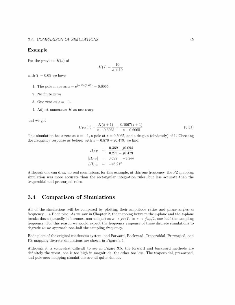
3.4. COMPARISON OF SIMULATIONS 45
Example
For the previous H(s) of
H(s) =10
s+ 10
with T = 0.05 we have
1. The pole maps as z = e(−10)(0.05) = 0.6065.
2. No finite zeros.
3. One zero at z = −1.
4. Adjust numerator K as necessary.
and we get
HPZ(z) =K(z + 1)
z − 0.6065=
0.1967(z + 1)
z − 0.6065(3.31)
This simulation has a zero at z = −1, a pole at z = 0.6065, and a dc gain (obviously) of 1. Checkingthe frequency response as before, with z = 0.878 + j0.479, we find
HPZ =0.369 + j0.094
0.271 + j0.479
|HPZ | = 0.692 = −3.2db
6 HPZ = −46.21o
Although one can draw no real conclusions, for this example, at this one frequency, the PZ mappingsimulation was more accurate than the rectangular integration rules, but less accurate than thetrapezoidal and prewarped rules.
3.4 Comparison of Simulations
All of the simulations will be compared by plotting their amplitude ratios and phase angles vsfrequency. . . a Bode plot. As we saw in Chapter 2, the mapping between the s-plane and the z-planebreaks down (actually it becomes non-unique) as s → jπ/T , or s → jωs/2, one half the samplingfrequency. For this reason we would expect the frequency response of these discrete simulations todegrade as we approach one-half the sampling frequency.
Bode plots of the original continuous system, and Forward, Backward, Trapezoidal, Prewarped, andPZ mapping discrete simulations are shown in Figure 3.5.
Although it is somewhat difficult to see in Figure 3.5, the forward and backward methods aredefinitely the worst, one is too high in magnitude, the other too low. The trapezoidal, prewarped,and pole-zero mapping simulations are all quite similar.
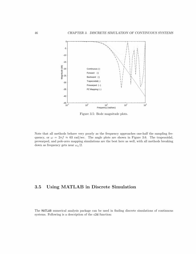
46 CHAPTER 3. DISCRETE SIMULATION OF CONTINUOUS SYSTEMS
10-1
100
101
102
103
-45
-40
-35
-30
-25
-20
-15
-10
-5
0
Frequency (rad/sec)
Mag
nitu
de (
db)
Continuous (-)
Forward (:)
Backward (:)
Trapezoidal(-.)
Prewarped (--)
PZ Mapping (-.)
Figure 3.5: Bode magnitude plots.
Note that all methods behave very poorly as the frequency approaches one-half the sampling fre-quency, or ω = 2πf ≈ 63 rad/sec. The angle plots are shown in Figure 3.6. The trapezoidal,prewarped, and pole-zero mapping simulations are the best here as well, with all methods breakingdown as frequency gets near ωs/2.
3.5 Using MATLAB in Discrete Simulation
The MATLAB numerical analysis package can be used in finding discrete simulations of continuoussystems. Following is a description of the c2d function:
3.5. USING MATLAB IN DISCRETE SIMULATION 47
10-1
100
101
102
103
-700
-600
-500
-400
-300
-200
-100
0
100
Frequency (rad/sec)
Ang
le (
degr
ees)
Figure 3.6: Bode angle plots.
C2D Conversion of continuous-time models to discrete time.
SYSD = C2D(SYSC,Ts,METHOD) converts the continuous-time LTI
model SYSC to a discrete-time model SYSD with sample time Ts.
The string METHOD selects the discretization method among the
following:
’zoh’ Zero-order hold on the inputs
’foh’ Linear interpolation of inputs (triangle appx.)
’imp’ Impulse-invariant discretization
’tustin’ Bilinear (Tustin) approximation
’prewarp’ Tustin approximation with frequency prewarping.
The critical frequency Wc (in rad/sec) is specified
as fourth input by
SYSD = C2D(SYSC,Ts,’prewarp’,Wc)
’matched’ Matched pole-zero method (for SISO systems only).
The default is ’zoh’ when METHOD is omitted.
The simulations methods that MATLAB supports that we have covered in this chapter are:
• tustin—trapezoidal (Tustin) integration rule
• prewarp—prewarped trapezoidal integration rule
• matched—pole-zero mapping

48 CHAPTER 3. DISCRETE SIMULATION OF CONTINUOUS SYSTEMS
The rectangular integration rules are not supported in MATLAB, they are not good performers anyway.The zoh simulation method is one we will examine in Chapter 4, I have chosen to omit it in thischapter. NOTE: MATLAB function c2d works with an “LTI system,” not the numerator anddenominator. A “transfer function” LTI system can be created using the TF function—this will bedone below (function c2dm still works with num and den, but c2d is preferred).
Example
Simulate the H(s) covered in the previous example using MATLAB. Recall that
H(s) =10
s+ 10(3.32)
1. Trapezoidal rule. The MATLAB script is shown below:
>> numc = [0 10]; % Define continuous numerator
>> denc = [1 10]; % Define continuous denominator
>> sysc = tf(numc,denc); % Create continuous LTI system
>> T = 0.05; % Define sampling period
>> sysd = c2d(sysc,T,’tustin’); % Discretize using trapezoidal approximation
>> sysd % Display the resulting discrete LTI system
Transfer function:
0.2 z + 0.2
-----------
z - 0.6
Sampling time: 0.05
2. Prewarped rule. The MATLAB script is shown below (the same continuous numerator anddenominator are used as before):
>>wp = 10; % Prewarping frequency of 10 rad/sec
>> sysp = c2d(sysc,T,’prewarp’,wp); % Discretize using prewarped
>> sysp % Display the resulting discrete LTI system
Transfer function:
0.2034 z + 0.2034
-----------------
z - 0.5932
Sampling time: 0.05
3.6. IMPLEMENTATION OF DIFFERENCE EQUATIONS IN REAL TIME 49
3. Pole-zero mapping :
>> syspz = c2d(sysc,T,’matched’); % Discretize using pole-zero mapping
>> syspz % Display resulting discrete system
Transfer function:
0.3935
----------
z - 0.6065
Sampling time: 0.05
3.5.1 Finding transfer function from LTI system
Sometimes you may need to extract the numerator and denominator from the LTI description ofthe system. Using the “pole-zero mapping” result obtained above, here’s how to use tfdata:
>> [numpz,denpz] = tfdata(syspz,’v’)
numpz =
0 0.3935
denpz =
1.0000 -0.6065
NOTE: Don’t forget the ’v’ or you’ll be in for grief!
3.6 Implementation of Difference Equations in Real Time
It is time to consider how to construct computer programs that will realize the difference equationswe obtain. Consider a general second-order discrete transfer function, written in z−1:
H(z) =Y (z)
U(z)=b0 + b1z
−1 + b2z−2
1− a1z−1 − a2z−2(3.33)
with corresponding difference equation
yk = a1yk−1 + a2yk−2 + b0uk + b1uk−1 + b2uk−2 (3.34)
We assume that in addition to A/D and D/A converters (and subroutines to use them) the computerhas a programmable real time clock such that a clock interrupt will occur every T seconds, where Tmay be set under program control. When a clock interrupt occurs, variable FLAG is set to one.

50 CHAPTER 3. DISCRETE SIMULATION OF CONTINUOUS SYSTEMS
3.6.1 Direct realization
Consider the following program structure:
10 read difference equation parameters and initialize variables;
20 set FLAG = 0;
30 select sample period, start clock;
40 if (FLAG == 1) print ("sampling period too short") and exit;
50 while (FLAG == 0) wait;
60 u(0) = adc_in(); % Read input u(k).
70 y(0) = a1*y(1) + a2*y(2) + b0*u(0) + b1*u(1) + b2*u(2); % compute y(k).
80 dac_out(y(0)); % Write output y(k) to D/A converter.
90 u(2) = u(1); % Propagate variables
100 u(1) = u(0); % backwards
110 y(2) = y(1); % for next
120 y(1) = y(0); % sample.
130 goto 40; % Execute continuously.
In the structure above the difference equation is explicitly calculated in line 70. While this approachis easy to follow, it is inefficient. The problem is the computational delay between the acquisition ofthe input sample in line 60 and the writing of the output sample in line 80. There are 5 multiplies,4 adds, and 1 assignment. Note that this computational delay is not the sampling period, and it isa delay which we have not modeled. Thus it should be minimized.
Also note the possibility of clock overrun in line 40. If variable FLAG has already been set by thetime we get back to the top of the loop, we are sampling too fast; the time allotted for the controlcomputation is too short. Either we sample slower, reduce the complexity of the control calculation,or get a faster computer.
3.6.2 Canonical realization
Consider the block diagram shown in Figure 3.7. Input u and output y are present, as are parametersak and bk. State variables x1 and x2 are new. While the general topic of state variable formulationwill be deferred until later in the course, it is necessary to illustrate a more efficient real timeimplementation. Note that the state variables are the outputs of the delay elements. . . this willalways be the case.
One should first verify that Figure 3.7 implements the difference equation of (3.34), this is left as anexercise for the student. A progam based on this block diagram is

3.6. IMPLEMENTATION OF DIFFERENCE EQUATIONS IN REAL TIME 51
uk
yk
b2 b1 b0
a2 a1
z−1z−1
+
+
+
+ +
+
+
x1x2
Figure 3.7: Observer canonical block diagram realization.
10 read difference equation parameters and initialize variables;
20 set FLAG = 0;
30 select sample period, start clock;
40 if (FLAG == 1) print ("sampling period too short") and exit;
50 while (FLAG == 0) wait;
60 u = adc_in();
70 y = x1 + b0*u;
80 dac_out(y);
90 x1 = x2 + b1*u + a1*y;
100 x2 = b2*u + a2*y;
130 goto 40;
Although the program loop is shorter overall, note particularly that the computational delay betweenline 60 and line 80 is now 1 multiply, 1 add, and 1 assignment. There is more computation afterwriting the output, but it’s not as critical there.
52 CHAPTER 3. DISCRETE SIMULATION OF CONTINUOUS SYSTEMS
Homework Problems
Problem 1.
The following transfer function is a lead network designed to add about 60o phase lead at ω1 = 3rad/sec:
H(s) =s+ 1
0.1s+ 1= 10
s+ 1
s+ 10
(a) For each of the following simulation methods compute and plot in the z-plane the pole andzero locations and compute the amount of phase lead given by the network at z1 = ejω1T . LetT = 0.25 sec.
(i) Forward rectangular rule.
(ii) Backward rectangular rule.
(iii) Trapezoidal rule.
(iv) Prewarped trapezoidal rule (use ω1 as the prewarping frequency).
(v) Pole-zero mapping.
(b) Plot the amplitude Bode plots of the continuous system and all simulations over the frequencyrange 0.1 ≤ ω ≤ 100 rad/sec.
(c) Develop a substitution rule based on the “parabolic” integration rule of Chapter 2 Problem 2.Use this rule to obtain a discrete simulation of the H(s) and compare the frequency responsewith the other methods.
Problem 2.
For this problem, construct the continuous transfer function G(s) of a second-order system withdamping ratio ζ = 0.2 and natural frequency ωn = 50 rad/sec, no zeros, and a dc gain of 1.
(a) Let the sampling frequency be 100 Hz. Find the following discrete simulations of G(s):
(i) Trapezoidal.
(ii) Prewarped (use ωn as the prewarping frequency).
(iii) Pole-zero mapping.
(b) Compare the Bode plots (both magnitude and phase plots) of the continuous G(s) and allG(z). Use frequency range 0.1 ≤ f ≤ 100 Hz.
(c) Compare the unit step response of the G(s) and any G(z).
3.6. IMPLEMENTATION OF DIFFERENCE EQUATIONS IN REAL TIME 53
Problem 3.
A notch filter is often useful in reducing the effect of an unwanted signal at a known constantfrequency, such as power line noise. The transfer function of a second-order notch filter is given by
H(s) =Y (s)
U(s)=
s2 + ω2o
s2 + 2ζωos+ w2o
where ζ =√
2/2 and ωo = notch frequency.
(a) Design a 60-Hz continuous notch filter H(s).
(b) Using a sampling frequency of 500 Hz, find the prewarped discrete simulation H(z) using thenotch frequency as the prewarped frequency.
(c) Draw Bode magnitude plots of H(s) and H(z) over 1 ≤ f ≤ 1000 Hz.
(d) Plot the time response of H(z) to an input which is the sum of an 11 Hz. sine wave and a 60Hz. sine wave, i.e.
u(t) = sin 2πf1t+ sin 2πf2t = sin 2π(11)t+ sin 2π(60)t
Show both input u(t) and output y(t) on your plot. Make sure H(z) has reached steady stateon your plot. Note the “start-up” transient.
(e) Draw a block diagram for H(z) in the observer canonical format of Figure 3.7. Assign statevariables xi and write a program in “pseudo-code” to realize this filter. What must theexcecution time of an arithmetic instruction be to implement this filter at a sampling rate of500 Hz? Assume equal time for multiply and add, and neglect assignments. Is this within thecapabilities of an “average” computer?

54 CHAPTER 3. DISCRETE SIMULATION OF CONTINUOUS SYSTEMS
Chapter 4
Sampled Data Systems
4.1 Introduction
In Chapter 2 we dealt with discrete systems only, covering difference equations and the z transform.Chapter 3 we did examine finding discrete simulations of continuous systems, but we did so from adiscrete perspective. In digital control systems where there are both discrete (the control algorithm)and continuous components (the plant), with a loop closure, it is imperative that we study theinteraction between discrete and continuous components with a more rigorous examination of theeffect of sampling. In comparison to Chapter 3, now we will work primarily in the continuous timedomain and use the Laplace transform.
4.2 The Sampling Process as Impulse Modulation
Consider a continuous signal which is sampled, as shown below, in which continuous signal r(t) is
A/D
T
r(t) r* (t)
sampled to produce a discrete signal which we will designate r∗(t). Note that this notation is asignificant departure from our previous treatment. Before, we have labeled the sampled signal rk, adiscrete variable. However, now we are claiming that the sampled signal can be called r∗(t), whichimplies we have a way of modeling this sampled signal in the time domain. We will obtain this timedomain model of a sampled signal using impulse modulation.
The sampled signal may be represented as the continuous signal convolved with a sequence of unitimpulses at the sample instants, which will result in the string of weighted impulses
r∗(t) = δ(t)r(0) + δ(t− T )r(T ) + δ(t− 2T )r(2T ) + . . . (4.1)
55
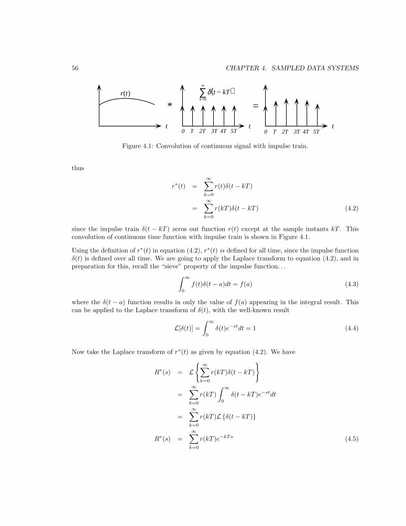
56 CHAPTER 4. SAMPLED DATA SYSTEMS
t t t
r(t)
0 T 2T 3T 4T 5T 0 T 2T 3T 4T 5T
* =
δ t − kT( )k =0
∞
∑
Figure 4.1: Convolution of continuous signal with impulse train.
thus
r∗(t) =∞∑k=0
r(t)δ(t− kT )
=
∞∑k=0
r(kT )δ(t− kT ) (4.2)
since the impulse train δ(t − kT ) zeros out function r(t) except at the sample instants kT . Thisconvolution of continuous time function with impulse train is shown in Figure 4.1.
Using the definition of r∗(t) in equation (4.2), r∗(t) is defined for all time, since the impulse functionδ(t) is defined over all time. We are going to apply the Laplace transform to equation (4.2), and inpreparation for this, recall the “sieve” property of the impulse function. . .∫ ∞
0
f(t)δ(t− a)dt = f(a) (4.3)
where the δ(t − a) function results in only the value of f(a) appearing in the integral result. Thiscan be applied to the Laplace transform of δ(t), with the well-known result
L[δ(t)] =
∫ ∞0
δ(t)e−stdt = 1 (4.4)
Now take the Laplace transform of r∗(t) as given by equation (4.2). We have
R∗(s) = L
∞∑k=0
r(kT )δ(t− kT )
=
∞∑k=0
r(kT )
∫ ∞0
δ(t− kT )e−stdt
=
∞∑k=0
r(kT )Lδ(t− kT )
R∗(s) =
∞∑k=0
r(kT )e−kTs (4.5)
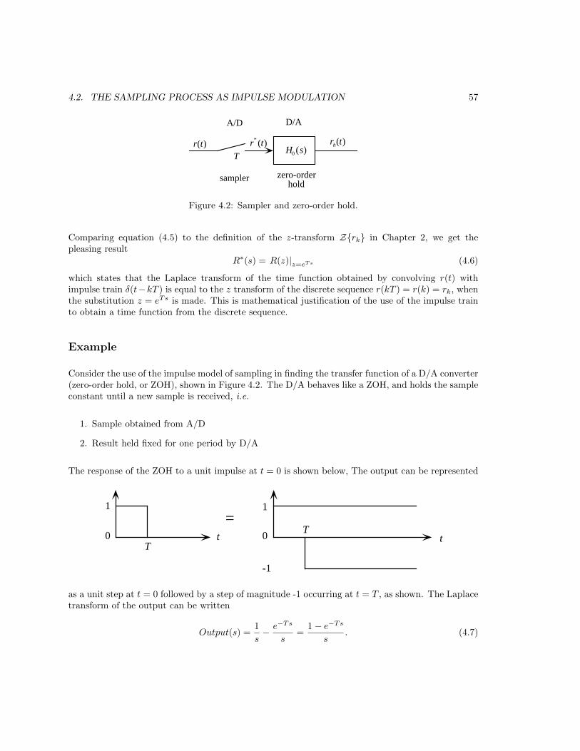
4.2. THE SAMPLING PROCESS AS IMPULSE MODULATION 57
A/D D/A
sampler zero-orderhold
Tr(t) r* (t)
H0 (s)rh(t)
Figure 4.2: Sampler and zero-order hold.
Comparing equation (4.5) to the definition of the z-transform Zrk in Chapter 2, we get thepleasing result
R∗(s) = R(z)|z=eTs (4.6)
which states that the Laplace transform of the time function obtained by convolving r(t) withimpulse train δ(t−kT ) is equal to the z transform of the discrete sequence r(kT ) = r(k) = rk, whenthe substitution z = eTs is made. This is mathematical justification of the use of the impulse trainto obtain a time function from the discrete sequence.
Example
Consider the use of the impulse model of sampling in finding the transfer function of a D/A converter(zero-order hold, or ZOH), shown in Figure 4.2. The D/A behaves like a ZOH, and holds the sampleconstant until a new sample is received, i.e.
1. Sample obtained from A/D
2. Result held fixed for one period by D/A
The response of the ZOH to a unit impulse at t = 0 is shown below, The output can be represented
t t
1
0 0
-1
=
T
T
1
as a unit step at t = 0 followed by a step of magnitude -1 occurring at t = T , as shown. The Laplacetransform of the output can be written
Output(s) =1
s− e−Ts
s=
1− e−Ts
s. (4.7)
58 CHAPTER 4. SAMPLED DATA SYSTEMS
Since the input has Laplace transform of 1 (unit impulse), the ratio of the Laplace transform of theoutput over that of the input yields the transfer function of the zero-order hold, which is
Ho(s) =1− e−sT
s(4.8)
We will use the transfer function of the ZOH, or D/A, given by equation (4.8) extensively in modelingsampled data systems.
4.3 Frequency Spectra of Sampled Signals—Aliasing
We have a method of mathematically representing continuous functions r(t) which have been sampled—this is the impulse sampling model given by equation (4.2). The question posed in this sectionis—what is the frequency spectrum of sampled signal r∗(t)? We will first find a Fourier series rep-resentation of the impulse train, use this in the expression for r∗(t), take the Laplace transform ofr∗(t), which is R∗(s), then use the fact that R∗(jω) = R∗(s)|s=jω.
4.3.1 Fourier transform and Fourier series
The Fourier transform and Fourier series will be necessary in the derivation to follow, we state thembelow, first the Fourier transform:
F (jω) =
∫ ∞−∞
f(t)e−jωtdt (4.9)
then the Fourier series (only applicable if f(t) is periodic):
f(t) =
∞∑n=−∞
Cnej(2πn/T )t (4.10)
where the Fourier coefficients are given by
Cn =1
T
∫ T2
−T2f(t)e−j(2πn/T )tdt (4.11)
In (4.10) and (4.11) T is the period of f(t). The double-sided expressions are given here, since themathematics is more straightforward than if single-sided were used.
Now, since the complete impulse train
∞∑k=−∞
δ(t− kT )
4.3. FREQUENCY SPECTRA OF SAMPLED SIGNALS—ALIASING 59
is periodic with period T , it can be represented by a Fourier Series;
∞∑k=−∞
δ(t− kT ) =
∞∑n=−∞
Cnej(2πn/T )t (4.12)
where the Fourier coefficients are given by
Cn =1
T
∫ T2
−T2
∞∑k=−∞
δ(t− kT )e−j(2πn/T )t. (4.13)
Although equation (4.13) looks formidable, the “sieving” property of the impulse function (and theonly impulse within the integration limits is at t = 0) yields a very simple result,
Cn =1
T
[e−j(2πn/T )(0)
]=
1
T(4.14)
Substituting the Fourier coefficients Cn from equation (4.14) into the Fourier series of (4.12), so
∞∑k=−∞
δ(t− kT ) =
∞∑n=−∞
1
Tej(2πn/T )t
=1
T
∞∑n=−∞
ejnωst (4.15)
where we have used the relation that sampling frequency ωs = 2π/T . Using the Fourier seriesexpression for the impulse train, we can express sampled signal r∗(t) as
r∗(t) =1
T
r(t)
∞∑n=−∞
ejnωst
(4.16)
The Laplace transform R∗(s) of sampled signal r∗(t) is
L[r∗(t)] =
∫ ∞−∞
1
T
r(t)
∞∑n=−∞
ejnωst
e−stdt
R∗(s) =1
T
∞∑n=−∞
∫ ∞−∞
r(t)ejnωste−stdt
=1
T
∞∑n=−∞
∫ ∞−∞
r(t)e−(s−jnωs)tdt
=1
T
∞∑n=−∞
R(s− jnωs) (4.17)

60 CHAPTER 4. SAMPLED DATA SYSTEMS
If F (s) is the Laplace transform of f(t), the Fourier transform F (jω) is given by
F (jω) = F (s)|s=jω (4.18)
thus
R∗(jω) =1
T
∞∑n=−∞
R(jω − jnωs) (4.19)
Equation (4.19) is a momentous result, it tells us that two things happen to the frequency spectrumof r(t) when it is sampled to become r∗(t):
1. The magnitude of the sampled spectrum is 1T that of the continuous spectrum, it is scaled by
1T .
2. The summation in (4.19) indicates that there are an infinite number of repeated spectra in thesampled signal, and they are repeated every ωs = 2π/T along the frequency axis.
Two Examples of Sampled Spectra
We will examine the effects of sampling on the amplitude spectra of two continuous functions.
Example 1. Consider continuous function r1(t) which has no frequency content above half thesampling frequency ωs/2. The original amplitude spectrum |R1(jω)| and the sampled spectrum|R∗1(jω)| are shown in Figure 4.3(a). The spectrum of the sampled r∗1(t) is scaled by 1/T andrepeated, but one can see the possibility of reconstructing by extracting the original single spectrumfrom the array of repeated spectra (Remember that all information present in r(t) is also present inR(jω), the original spectrum).
Example 2. Now consider function r2(t) which has frequency content above half the samplingfrequency ωs/2. The same scaling and repetition occurs in the sampled spectrum, but this timedue to the addition of the overlapping spectra in Figure 4.3(b) there is no chance of recovering theoriginal spectrum after sampling.
Another phenomenon is shown in Figure 4.3(b), that of aliasing, illustrated at the frequency markedωo. The magnitude of the overall spectrum at ωo is due to two different spectra, the “original”spectrum R(jωo), and the repeated spectrum centered at ωs = 2π/T . The value of the magnitudefrom the repeated spectrum is R(jωa), where ωa = ωo − ωs. This frequency, ωa, which shows up atωo after sampling, is called an alias of ωo.
Aliasing means that two different sinusoids have identical samples, and we cannot distinguish betweenthem from their samples. When experimental data are to be sampled, it is essential that an “anti-aliasing” analog filter be used before sampling to filter out frequencies above one-half the samplingfrequency (called the Nyquist frequency). Otherwise, frequencies above the Nyquist frequency in

4.3. FREQUENCY SPECTRA OF SAMPLED SIGNALS—ALIASING 61
R1( jω) T R1* ( jω )
12ω s− 1
2ωs − 32ωs
32ω s
12ω s− 1
2ωs0 0 ω s−ω s 2ω s
ω ω
(a) Non-overlapping spectra.
12ω s− 1
2ωs − 32ωs
32ω s
12ω s− 1
2ωs0 0 ω s−ω s 2ω s
ω ω
R2( jω ) T R2*( jω )
false spectrumdue to additionof overlapping
spectra
ωo
ωa
(b) Overlapping spectra showing contamination.
Figure 4.3: Frequency spectra of two signals.
the continuous signal will erroneously appear as lower frequencies after sampling. This is shown inFigure 4.4, where fo = 7
8 Hz, and sampling frequency fs = 1 Hz. Then fo appears at
fa =7
8− 1 = −1
8(4.20)
The significance of the negative frequency is that the 18 -Hz sinusoid in Figure 4.4 is the negative of
the original 78 -Hz sinusoid.
Another way of looking at aliasing is that the act of sampling causes a “reflecting” of frequenciesaround the Nyquist frequency (fs/2); refer to the dashed lines in Figure 4.8 where fs = 500 Hz, anda component at 100 Hz will also show up at 400 Hz, 600 Hz, 900 Hz, 1100 Hz, and so on.
Sampling Theorem
This can be viewed as:
What is the highest frequency we can allow in r(t) so that aliasing will not occur?
From inspection of Figure 4.3 it is clear that if R(jω) has components above ωs/2 or π/T , thenspectral overlap and aliasing will occur. The sampling theorem is
To recover a signal from its samples, you must sample at least twice the highest frequencyin the original signal. If R(jω) = 0 for ω ≥ ωs
2 , there will be no aliasing, and the originalsignal may be recovered from R∗(jω), the Fourier transform of the samples (but not inreal time!).

62 CHAPTER 4. SAMPLED DATA SYSTEMS
0 2 4 6 8-1
-0.5
0
0.5
1
Time (seconds)Figure 4.4: Plot of two sinusoids which have identical values at thesampling intervals: an example of aliasing.
4.4 Desampling or Signal Reconstruction
This is the reverse operation of sampling. Given the samples, how can we reconstruct a continuoussignal? The samping theorem says that under the right conditions (no aliasing) it is possible torecover the original signal from the samples, although I have indicated this is impossible in realtime. This section presents one method for such a reconstruction.
We will use an ideal filter. Consider recovering R(jω) from R∗(jω). This may be done by passingR∗(jω) through an ideal low pass filter L(jω), with magnitude
|L(jω)| = T, − πT≤ ω ≤ π
T(4.21)
|L(jω)| = 0, |ω| > π
T(4.22)
The filter amplitude in equation (4.21) will pass the original spectrum, while that in equation (4.22)will reject the repeated spectra. This is shown in Figure 4.5.
4.4.1 Impulse response of the Ideal Desampling Filter
The ideal sampling filter L(jω) can recover R(jω) from R∗(jω) using
R(jω) = L(jω)R∗(jω) (4.23)
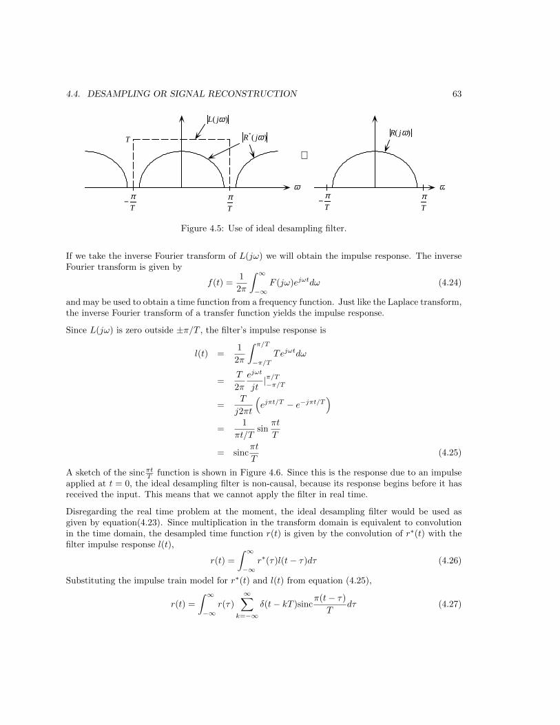
4.4. DESAMPLING OR SIGNAL RECONSTRUCTION 63
ω ω
L( jω )
R*( jω )R( jω)
⇒
−πT
πT
πT
−πT
T
Figure 4.5: Use of ideal desampling filter.
If we take the inverse Fourier transform of L(jω) we will obtain the impulse response. The inverseFourier transform is given by
f(t) =1
2π
∫ ∞−∞
F (jω)ejωtdω (4.24)
and may be used to obtain a time function from a frequency function. Just like the Laplace transform,the inverse Fourier transform of a transfer function yields the impulse response.
Since L(jω) is zero outside ±π/T , the filter’s impulse response is
l(t) =1
2π
∫ π/T
−π/TTejωtdω
=T
2π
ejωt
jt|π/T−π/T
=T
j2πt
(ejπt/T − e−jπt/T
)=
1
πt/Tsin
πt
T
= sincπt
T(4.25)
A sketch of the sincπtT function is shown in Figure 4.6. Since this is the response due to an impulseapplied at t = 0, the ideal desampling filter is non-causal, because its response begins before it hasreceived the input. This means that we cannot apply the filter in real time.
Disregarding the real time problem at the moment, the ideal desampling filter would be used asgiven by equation(4.23). Since multiplication in the transform domain is equivalent to convolutionin the time domain, the desampled time function r(t) is given by the convolution of r∗(t) with thefilter impulse response l(t),
r(t) =
∫ ∞−∞
r∗(τ)l(t− τ)dτ (4.26)
Substituting the impulse train model for r∗(t) and l(t) from equation (4.25),
r(t) =
∫ ∞−∞
r(τ)
∞∑k=−∞
δ(t− kT )sincπ(t− τ)
Tdτ (4.27)

64 CHAPTER 4. SAMPLED DATA SYSTEMS
0
t
1
Figure 4.6: Sinc function. . . impulse response of ideal desampling filter.
or, using the “sieving” property of the δ(t− a),
r(t) =
∞∑k=−∞
r(kT )sincπ(t− kT )
T(4.28)
Equation (4.28) shows how to reconstruct the (band-limited. . . no aliasing!) function r(t) from itssamples r∗(t). The sinc() function fills in the gaps between samples.
4.4.2 The ZOH as a Desampling Filter
The ideal desampling filter, being non-causal, cannot be used in real time, so we will examine thebehavior of a zero-order hold, which is exactly the behavior of a D/A converter. Recall the transferfunction of a ZOH:
Ho(s) =1− e−sT
s(4.29)
The frequency behavior of Ho(s) is Ho(jω),
Ho(jω) =1− e−jωT
jω(4.30)
Multiplying numerator and denominator of (4.30) by ejωT/2, the magnitude of (4.30) is
|H(jω)| =
∣∣∣∣ejωT/2 − e−jωT/2jωejωT/2
∣∣∣∣= T
∣∣∣∣ sinωT/2ωT/2
∣∣∣∣= T
∣∣∣∣sincωT
2
∣∣∣∣ (4.31)

4.4. DESAMPLING OR SIGNAL RECONSTRUCTION 65
ω
ωωs =
2πT
2ωs
Ho
∠Ho
0
−180°
T
Figure 4.7: Frequency response of zero-order hold.
and the angle of (4.30) is
6 Ho(jω) = 6ejωT/2 − e−jωT/2
jωejωT/2
= 62 sinωT/2
ωejωT/2
= −ωT2
(4.32)
A plot of the frequency characteristics of the ZOH are shown in Figure 4.7. The ZOH is a low-pass filter, at least an approximation of the ideal desampling filter, and has linear phase lag withfrequency. This phase lag can be viewed as the destabilizing effect of information loss at low samplingfrequencies. The DC magnitude of T of the ZOH compensates for the frequency scaling of 1/Tincurred by sampling.
Aliasing Lab Demonstration
The block diagram below shows a laboratory setup with an A/D converter, computer program whichpasses the numbers “straight through,” and D/A converter (or ZOH) at the output. Variables

66 CHAPTER 4. SAMPLED DATA SYSTEMS
r(t), r∗(t) represent the continuous and sampled inputs, while rh(t) is the desampled output. Thesampling frequency will be 500 Hz, or T = 0.002. A sinusoidal function generator will be used to
A/D Computer D/A
ZOHT
r(t) r* (t)1
r* (t) rh(t)
provide the input, sor(t) = ro sinωt
and the frequency spectrum R(jω) will be a single line at ω. The frequency spectrum of rh(t) is
Rh(jω) = R∗(jω)Ho(jω)
with magnitude
|Rh(jω)| = 1
T
∞∑n=−∞
|R(jω − jnωs)|T∣∣∣∣sinc
ωT
2
∣∣∣∣The process of sampling will cause the repeated spectra shown in Figure 4.3, but their magnitudewill be attenuated by the amplitude ratio of the ZOH shown in Figure 4.7.
The spectral amplitudes of the continuous input and the sampled and reconstructed output will bedisplayed on a spectrum analyzer. The expected amplitudes at several frequencies are shown in theaccompanying table. Signals at these frequencies will be attenuated accordingly.
f (Hz) ω ωT/2 sinc(ωT/2) db
50 314 0.314 0.984 -0.14100 628 0.628 0.936 -0.58150 942 0.942 0.858 -1.33200 1257 1.257 0.757 -2.42300 1885 1.885 0.505 -5.94
The magnitude of the ZOH frequency response at a sampling frequency of 500 Hz is shown in theplot. If the input is a sinusoid at 100 Hz, there will repeated spectra at 400, 600, 900, 1100. . . Hz.The discrete spectral lines are shown as solid lines, while their attenuated versions (which are whatwe actually see in Rh(jω) are shown by dashed lines.
4.5 Block Diagram Analysis
In this section methods to reduce block diagrams of sampled data systems will be covered. Unlikecontinuous systems, sampled data systems contain samplers (A/D converters) and discrete elements(computer programs). In terms of continuous component connections, there are really only twopossibilities:
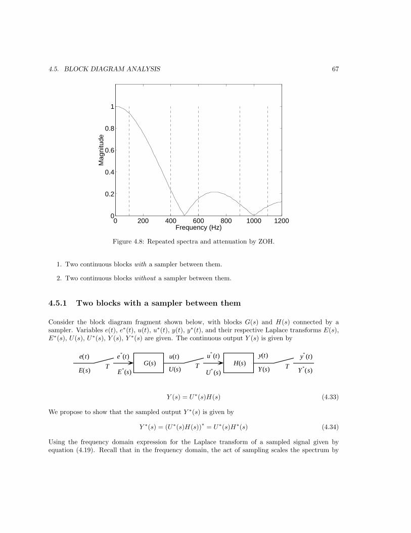
4.5. BLOCK DIAGRAM ANALYSIS 67
0 200 400 600 800 1000 12000
0.2
0.4
0.6
0.8
1
Frequency (Hz)
Mag
nitu
de
Figure 4.8: Repeated spectra and attenuation by ZOH.
1. Two continuous blocks with a sampler between them.
2. Two continuous blocks without a sampler between them.
4.5.1 Two blocks with a sampler between them
Consider the block diagram fragment shown below, with blocks G(s) and H(s) connected by asampler. Variables e(t), e∗(t), u(t), u∗(t), y(t), y∗(t), and their respective Laplace transforms E(s),E∗(s), U(s), U∗(s), Y (s), Y ∗(s) are given. The continuous output Y (s) is given by
e( t) e*(t) u(t) u* (t) y(t) y* (t)
T T TG(s) H(s)E(s) E*(s) U* (s) Y *(s)Y (s)U(s)
Y (s) = U∗(s)H(s) (4.33)
We propose to show that the sampled output Y ∗(s) is given by
Y ∗(s) = (U∗(s)H(s))∗
= U∗(s)H∗(s) (4.34)
Using the frequency domain expression for the Laplace transform of a sampled signal given byequation (4.19). Recall that in the frequency domain, the act of sampling scales the spectrum by

68 CHAPTER 4. SAMPLED DATA SYSTEMS
1/T and causes infinite repeated duplicate spectra at ωs intervals. Hence Y ∗(s) is just Y (s) sampled,or
Y ∗(s) = U∗(s)H(s)∗
=1
T
∞∑n=−∞
U∗(s− jnωs)H(s− jnωs) (4.35)
and
U∗(s) =1
T
∞∑k=−∞
U(s− jkωs) (4.36)
so
U∗(s− jnωs) =1
T
∞∑k=−∞
U(s− jkωs − jnωs) (4.37)
Let k = l − n, or k + n = l, then
U∗(s− jnωs) =1
T
∞∑l=−∞
U(s− jlωs)
= U∗(s) (4.38)
The spectrum of sampled variable U∗ can be shifted an integral number of periods ωs because itsspectrum is periodic with this “period.”
We can make use of this property in equation (4.35), substituting (4.38), so
Y ∗(s) =1
T
∞∑n=−∞
U∗(s− jnωs)H(s− jnωs)
= U∗(s)1
T
∞∑n=−∞
H(s− jnωs)
= U∗(s)H∗(s) (4.39)
The result we were after was Y ∗(s) = U∗(s)H∗(s). This could have also been applied to block G(s)and input E∗(s) to yield
U∗(s) = E∗(s)G∗(s) (4.40)
Relations (4.39) and (4.40) can be combined to yield
Y ∗(s) = E∗(s)G∗(s)H∗(s) = E∗G∗H∗ (4.41)
The point in equation (4.41) is that blocks G and H “come apart,” we have G∗H∗, not (GH)∗. Thisis due to the sampler between them.

4.5. BLOCK DIAGRAM ANALYSIS 69
The “*” transform and z-transform It is worthwhile to distinguish the “*” transform and thez-transform. Using equation (4.6) we can find the Y (z) from Y ∗(s) by
Y (z) = Y ∗(s)|esT=z (4.42)
It is important to understand the inverse of both Y ∗(s) and Y (z):
L−1 [U∗(s)] ⇒ sequence of impulses with intensities u(kT )
Z−1 [U(z)] ⇒ sequence of values uk (4.43)
In most of the transform-based design work to follow, we will use Y (z) rather than Y ∗(s) becauseit is more concise.
4.5.2 Two blocks without a sampler between them
Without going into detail, using a similar derivation (but somewhat simpler) as above, it can beshown that for the block connection below that Y ∗(s) 6= U∗(s)H∗(s), but rather
y(t) y* (t)
TH(s)Y *(s)Y (s)
e( t) e*(t) u(t)
T G(s)E(s) E*(s) U(s)
Y ∗(s) = UH∗(s) (4.44)
Likewise,U(s) = E∗(s)G(s) (4.45)
Equations (4.44) and (4.45) can be combined to yield
Y ∗(s) = E∗(s)G(s)H(s)∗ = E∗(s)G(s)H(s)∗ = E∗GH∗ (4.46)
Comparing (4.41) and (4.46) it can be seen that without a sampler between G and H they do not“come apart.”
Block Diagram Reduction Procedure
In reducting block diagrams of sampled-data systems, the basic principle is
Solve for the variables which are sampled!
You will usually get simpler algebraic reduction. In most cases in this course we want transferfunctions relating sampled output to sampled input, rather than continuous variables. Now forsome examples. . .

70 CHAPTER 4. SAMPLED DATA SYSTEMS
A/D Computer D/A (ZOH) Plant
r e e*
T
m* u yD* (s)
1 − e−Ts
sG(s)
+
-
Example 1
In the block diagram shown below, the error signal e(t) is sampled by the A/D converter, thereis a computer program modeled as discrete transfer function D∗(s) (note that it could have been,and will soon be modeled as D(z)), D/A converter modeled as a ZOH, and finally a continuousplant G(s). In every case the “*” notation signifies a sampled variable with the impulse modulationsampling model.
The error signal is sampled, so start with that. . .
E(s) = R(s)− Y (s) (4.47)
M∗(s) = E∗(s)D∗(s) (4.48)
U(s) = M∗(s)
[1− e−Ts
s
](4.49)
Y (s) = G(s)U(s) (4.50)
We’d like to relate the samples of the output Y ∗ (s) to samples of the input R∗(s). We can simply“star” each transform,
E∗ = R∗ − Y ∗ (4.51)
M∗ = E∗D∗ (4.52)
U∗ = M∗ (since samples of u and m are the same) (4.53)
Y ∗ = [GU ]∗ (4.54)
Equations (4.49) and (4.54) give us
Y ∗ =
[GM∗
(1− e−Ts
s
)]∗(4.55)
where we should remember that the “star” operation is really the act of impulse-modulating, thenLaplace transforming.
Anyway, in equation (4.55) both M∗ and (1 − e−Ts) may be taken outside the “*” since they’realready impulse sampled (an easy way to check this is to see that they both have periodic spectra).
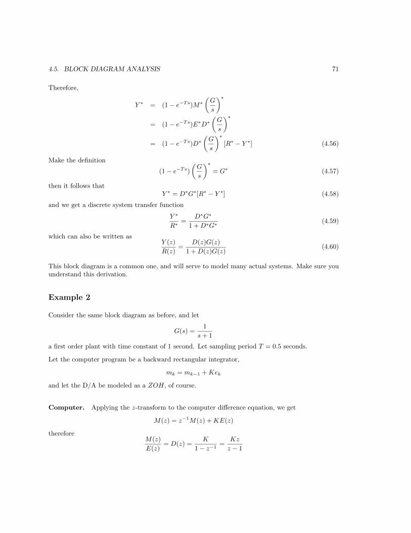
4.5. BLOCK DIAGRAM ANALYSIS 71
Therefore,
Y ∗ = (1− e−Ts)M∗(G
s
)∗= (1− e−Ts)E∗D∗
(G
s
)∗= (1− e−Ts)D∗
(G
s
)∗[R∗ − Y ∗] (4.56)
Make the definition
(1− e−Ts)(G
s
)∗= G∗ (4.57)
then it follows thatY ∗ = D∗G∗[R∗ − Y ∗] (4.58)
and we get a discrete system transfer function
Y ∗
R∗=
D∗G∗
1 +D∗G∗(4.59)
which can also be written asY (z)
R(z)=
D(z)G(z)
1 +D(z)G(z)(4.60)
This block diagram is a common one, and will serve to model many actual systems. Make sure youunderstand this derivation.
Example 2
Consider the same block diagram as before, and let
G(s) =1
s+ 1
a first order plant with time constant of 1 second. Let sampling period T = 0.5 seconds.
Let the computer program be a backward rectangular integrator,
mk = mk−1 +Kek
and let the D/A be modeled as a ZOH, of course.
Computer. Applying the z-transform to the computer difference equation, we get
M(z) = z−1M(z) +KE(z)
thereforeM(z)
E(z)= D(z) =
K
1− z−1=
Kz
z − 1
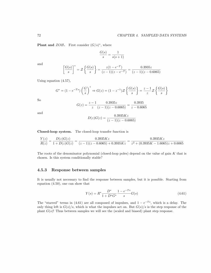
72 CHAPTER 4. SAMPLED DATA SYSTEMS
Plant and ZOH. First consider (G/s)∗, where
G(s)
s=
1
s(s+ 1)
and [G(s)
s
]∗= Z
G(s)
s
=
z(1− e−T )
(z − 1)(z − e−T )=
0.3935z
(z − 1)(z − 0.6065)
Using equation (4.57),
G∗ = (1− e−Ts)(G
s
)∗⇒ G(z) = (1− z−1)Z
G(s)
s
=z − 1
zZG(s)
s
So
G(z) =z − 1
z
0.3935z
(z − 1)(z − 0.6065)=
0.3935
z − 0.6065
and
D(z)G(z) =0.3935Kz
(z − 1)(z − 0.6065)
Closed-loop system. The closed-loop transfer function is
Y (z)
R(z)=
D(z)G(z)
1 +D(z)G(z)=
0.3935Kz
(z − 1)(z − 0.6065) + 0.3935Kz=
0.3935Kz
z2 + (0.3935K − 1.6065)z + 0.6065
The roots of the denominator polynomial (closed-loop poles) depend on the value of gain K that ischosen. Is this system conditionally stable?
4.5.3 Response between samples
It is usually not necessary to find the response between samples, but it is possible. Starting fromequation (4.50), one can show that
Y (s) = R∗D∗
1 +D∗G∗1− e−Ts
sG(s) (4.61)
The “starred” terms in (4.61) are all composed of impulses, and 1 − e−Ts, which is a delay. Theonly thing left is G(s)/s, which is what the impulses act on. But G(s)/s is the step response of theplant G(s)! Thus between samples we will see the (scaled and biased) plant step response.

4.5. BLOCK DIAGRAM ANALYSIS 73
Homework Problems
Problem 1.
Using MATLAB, verify the Fourier series expansion of the impulse train given in equation (4.15) byplotting a few periods of the Fourier series for several numbers of terms, such as 3,10, 100, etc.
Problem 2.
Sketch the step response y(t) of the system shown below for the three samples k = 0, 1, 2. Usesample period T = 1.
1 − e−Ts
s
1
s + 1
r(t) y(t)
T+−
ZOH G(s)
Problem 3.
Assume the plant transfer functions below are preceded by a zero-order hold. Compute the equivalentdiscrete transfer function G(z). Use sampling period T = 1. I would like you to find the G(z)by hand, then compare your results to MATLAB. Note: This is the “zero-order hold” discretesimulation method that we didn’t cover in Chapter 3.
(a) G(s) =1
s2
(b) G(s) =1
s(s+ 1)
(c) G(s) =1
s2 − 1
Problem 4.
Using a MATLAB program, verify the ideal reconstruction method given in equation (4.28). Foryour sampled data, use 6 samples (k = 0...5) of a 1 Hz sine wave with T = 0.2. Compute a full periodof the reconstructed continuous signal at a much finer time step, such as 0.01 second. Compare thereconstructed signal using only 6 samples with the original continuous signal. It really works!

74 CHAPTER 4. SAMPLED DATA SYSTEMS

Chapter 5
Design Using Transform Methods
5.1 Introduction
In this chapter we will discuss digital control system design using transform-based methods. Aswith continuous controllers, the goal of design is to transform the behavior from unacceptable toacceptable. Specific design specifications are, of course, different from application to application. Wewill take an application of controlling the azimuth angle of a large antenna, and use this applicationto illustrate some basic performance issues:
1. Steady-state accuracy.
2. Transient response.
3. Disturbance rejection
4. Control effort and gain distribution
5. Sensitivity to parameter changes
A typical control system application will involve all of these issues. We nearly always want adequatesteady-state accuracy; transient response is also usually important. Disturbance rejection must beaddressed if the plant is subject to disturbance inputs during operation. Control effort and gaindistribution must be analyzed to preclude component saturation, and gain distribution specificallytakes on greater importance in digital controllers, with A/D and D/A resolution involved. Finally,component parameters will change, a thorough design will examine the system behavior with thesechanges.
Pole-placement design will be used in this chapter, in which the designer chooses the locations ofthe system closed-loop poles, then designs a controller to place them there. The root locus methodis a pole-placement method for transform-based design. The mathematics of the root locus method
75

76 CHAPTER 5. DESIGN USING TRANSFORM METHODS
are independent of complex domain, thus the technique is the same whether used in the s-plane orz-plane. The reader should review the coverage of the root-locus method in an introductory controlstextbook.
Frequency-domain methods (Bode and Nyquist plots), which are frequently used for the design ofcontinuous control systems, require some adaptation when used with digital control systems, andwill not be discussed in this chapter.
There are two strategies for pole-placement transform-based design, which are:
• Design in the s-plane by “discrete equivalent”
• Direct Design in the z-plane.
In the first method, we design a continuous controller in the s-plane, using methods from continuoussystem modeling and analysis, obtaining some compensator Gc(s). To implement this in a digitalcontrol system, use one of the methods of Chapter 3 to get a discrete equivalent Gc(z), then use thisin the digital control system. Note that this method never considers the effect of sampling on theplant. This will cause the resulting system to be in error. The extent of this error depends mainlyon how fast you sample. If sampling is “fast” there will be less error; if sampling is slower—moreerror.
In the second method, “direct” design in the z-plane, we get a discrete domain model of the plantdynamics. Then the controller design is done in the sampled domain, the z-plane, from the outset.In this case the design is “guaranteed” to work, since we have considered the effect of sampling onthe plant.
5.2 Example System and Specifications
Consider the control of the azimuth pointing angle of a large antenna, such as a radio telescope.This can be considered angular position control of a large rotary inertia. The actuator will be a DCelectric motor. The “plant” will be taken as the combination of actuator and antenna. The equationof motion of the plant is
Jθ +Bθ = T + Tw (5.1)
where
θ = antenna angle (controlled variable
J = total rotary inertia
B = total viscous friction (includes back emf)
T = motor torque
Tw = wind (disturbance) torque
A block diagram of the plant is shown in Figure 5.1. Assume that J/B = 10 seconds. This is a
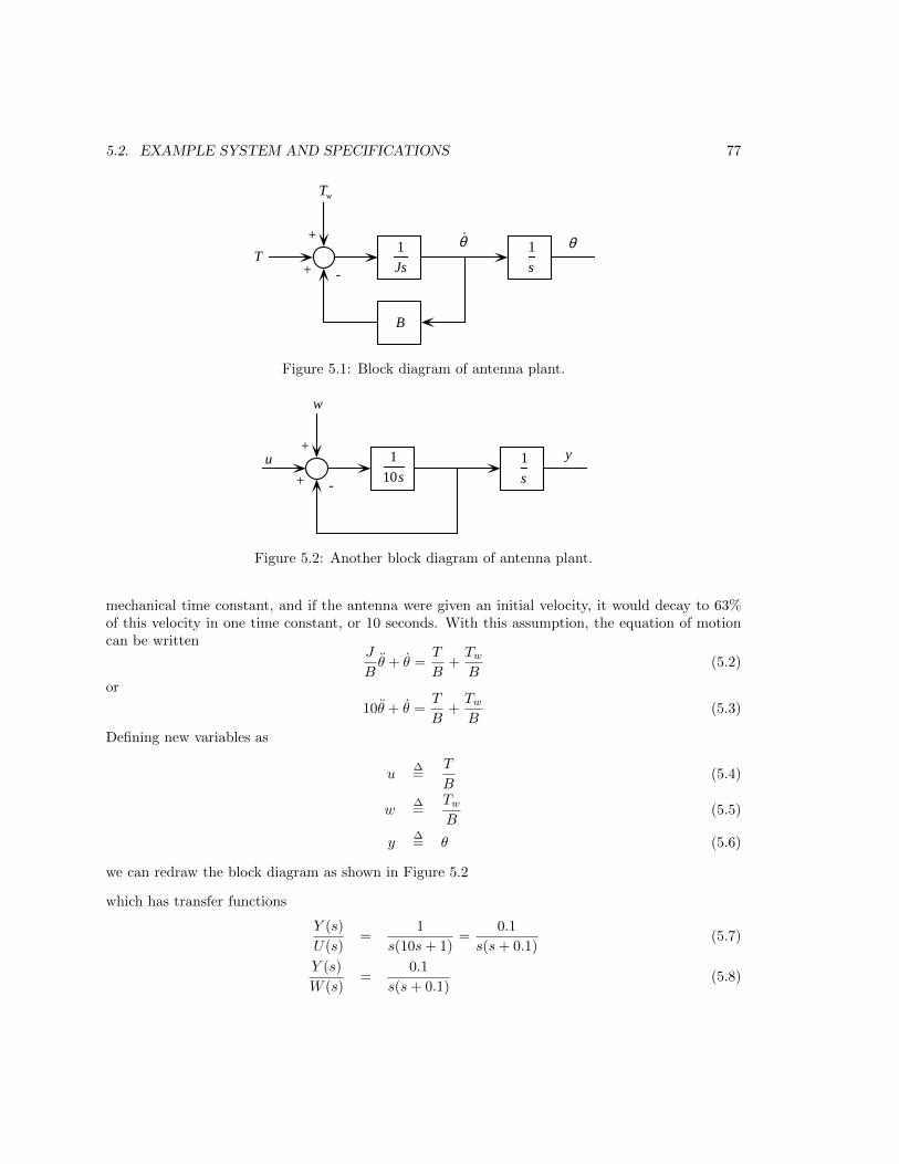
5.2. EXAMPLE SYSTEM AND SPECIFICATIONS 77
+ -
+
T
Tw
1
Js
1
s
B
θθ
Figure 5.1: Block diagram of antenna plant.
+ -
+1
su
w
y1
10s
Figure 5.2: Another block diagram of antenna plant.
mechanical time constant, and if the antenna were given an initial velocity, it would decay to 63%of this velocity in one time constant, or 10 seconds. With this assumption, the equation of motioncan be written
J
Bθ + θ =
T
B+TwB
(5.2)
or
10θ + θ =T
B+TwB
(5.3)
Defining new variables as
u∆=
T
B(5.4)
w∆=
TwB
(5.5)
y∆= θ (5.6)
we can redraw the block diagram as shown in Figure 5.2
which has transfer functions
Y (s)
U(s)=
1
s(10s+ 1)=
0.1
s(s+ 0.1)(5.7)
Y (s)
W (s)=
0.1
s(s+ 0.1)(5.8)

78 CHAPTER 5. DESIGN USING TRANSFORM METHODS
R E U
W
Y+
-D(z) G(z)
+
+
Figure 5.3: Block diagram for ss error analysis.
Our controller for this plant will accept a reference position (set point) θr, and will compute controlforce T such that the tracking error e = θr − θ satisfies specifications.
5.2.1 Steady-State Accuracy
For this antenna control system, the steady-state accuracy specification is given as follows:
For reference input θr(t) = 0.01t (this is 34o/minute) after transients die out, steady-stateerror θr − θ < 0.01 rad.
In general, tracking error comes from two sources: changes in the reference input and the onsetof disturbances. As you will recall from your continuous control course, system Type determinessteady-state behavior,
Type 0. Finite steady-state error when setpoint is a constant position (step input).
Type 1. Finite steady-state error when setpoint is a constant velocity (ramp input), and zero errorwhen setpoint is constant position.
Type 2. Finite steady-state error when setpoint is a constant acceleration (parabolic input), andzero error when setpoint is constant velocity or position.
Note that “position, velocity, and acceleration” refer to the rates of change of the setpoint variable,not the variable itself (the setpoint could be a temperature, for example).
To compute the steady-state error, consider the system block diagram shown in Figure 5.3. Thisblock diagram is in sampled form; all variables and transfer functions are functions of z. We will letthe disturbance w be zero, it is shown in Figure 5.3 for generality. The system equations are
E(z) = R(z)−G(z)D(z)E(z) (5.9)
so
E(z) =R(z)
1 +G(z)D(z)(5.10)

5.2. EXAMPLE SYSTEM AND SPECIFICATIONS 79
Step input, position error doefficient. Let r(t) be a step of magnitude ro, thus
R(z) =roz
z − 1(5.11)
so the error is
E(z) =roz
z − 1
1
1 +G(z)D(z)(5.12)
Now apply the final value theorem to E(z):
e(∞) = limz→1
(z − 1)roz
z − 1
1
1 +G(z)D(z)
=ro
1 +G(1)D(1)(5.13)
∆=
ro1 +Kp
(5.14)
and the position error coefficient is given by
Kp∆= G(1)D(1) (5.15)
and the steady-state error is given by equation (5.14).
The position error coefficient Kp varies with system Type as:
Type 0: G(z)D(z) has no poles at z = 1, Kp is finite.
Type 1: G(z)D(z) has one pole at z = 1, Kp =∞.
Type 2: G(z)D(z) has two poles at z = 1, Kp =∞.
Ramp input, velocity error coefficient. Here consider a ramp input of slope vo, given by
R(z) =voTz
(z − 1)2(5.16)
then the error is
E(z) =voTz
(z − 1)2
1
1 +G(z)D(z)(5.17)
The steady-state error is
e(∞) = limz→1
voTz
(z − 1)[1 +G(z)D(z)]
∆=
voKv
(5.18)
thus
Kv = limz→1
(z − 1)[1 +G(z)D(z)]
Tz
= limz→1
(z − 1)G(z)D(z)
Tz(5.19)
The velocity error coefficient Kv varies with system Type as:
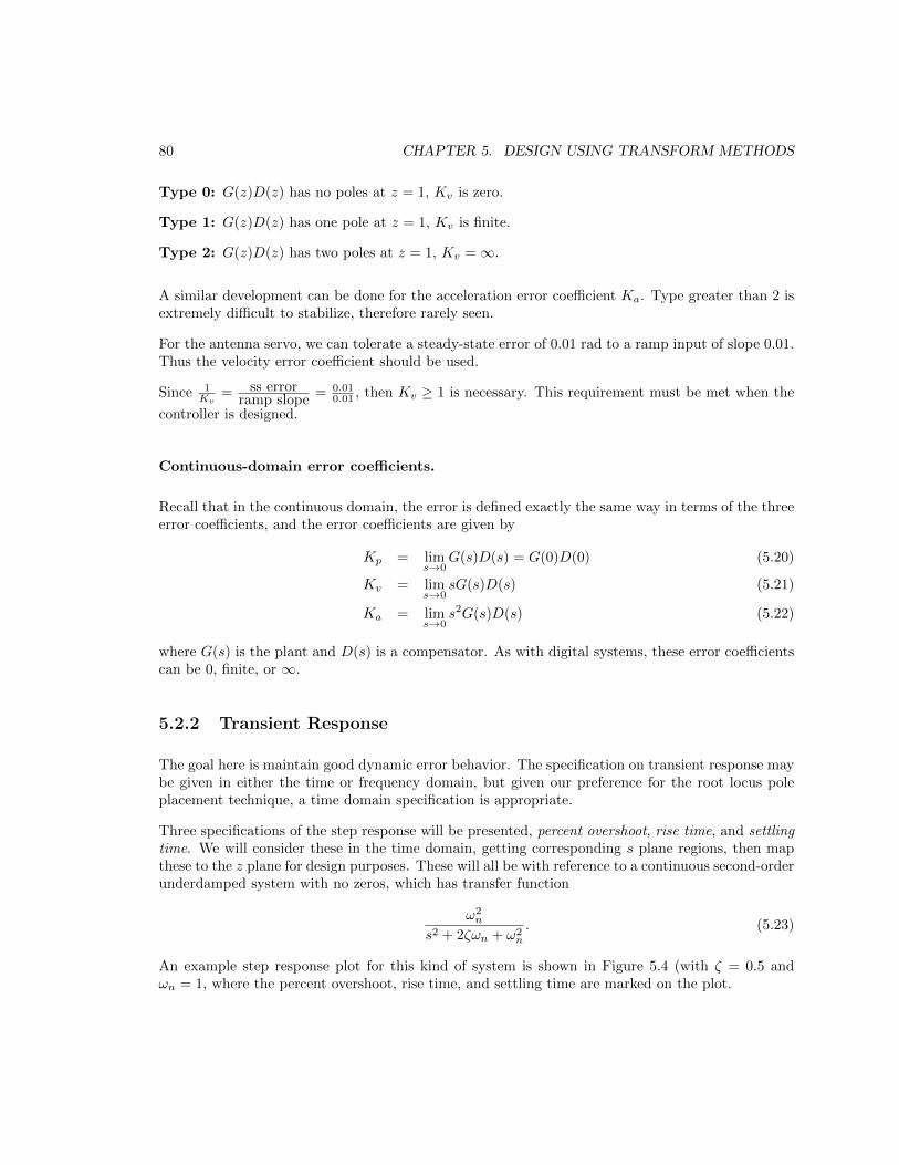
80 CHAPTER 5. DESIGN USING TRANSFORM METHODS
Type 0: G(z)D(z) has no poles at z = 1, Kv is zero.
Type 1: G(z)D(z) has one pole at z = 1, Kv is finite.
Type 2: G(z)D(z) has two poles at z = 1, Kv =∞.
A similar development can be done for the acceleration error coefficient Ka. Type greater than 2 isextremely difficult to stabilize, therefore rarely seen.
For the antenna servo, we can tolerate a steady-state error of 0.01 rad to a ramp input of slope 0.01.Thus the velocity error coefficient should be used.
Since 1Kv
= ss errorramp slope
= 0.010.01 , then Kv ≥ 1 is necessary. This requirement must be met when the
controller is designed.
Continuous-domain error coefficients.
Recall that in the continuous domain, the error is defined exactly the same way in terms of the threeerror coefficients, and the error coefficients are given by
Kp = lims→0
G(s)D(s) = G(0)D(0) (5.20)
Kv = lims→0
sG(s)D(s) (5.21)
Ka = lims→0
s2G(s)D(s) (5.22)
where G(s) is the plant and D(s) is a compensator. As with digital systems, these error coefficientscan be 0, finite, or ∞.
5.2.2 Transient Response
The goal here is maintain good dynamic error behavior. The specification on transient response maybe given in either the time or frequency domain, but given our preference for the root locus poleplacement technique, a time domain specification is appropriate.
Three specifications of the step response will be presented, percent overshoot, rise time, and settlingtime. We will consider these in the time domain, getting corresponding s plane regions, then mapthese to the z plane for design purposes. These will all be with reference to a continuous second-orderunderdamped system with no zeros, which has transfer function
ω2n
s2 + 2ζωn + ω2n
. (5.23)
An example step response plot for this kind of system is shown in Figure 5.4 (with ζ = 0.5 andωn = 1, where the percent overshoot, rise time, and settling time are marked on the plot.

5.2. EXAMPLE SYSTEM AND SPECIFICATIONS 81
0 2 4 6 8 100
0.2
0.4
0.6
0.8
1
1.2
Time (seconds)
PO
tr
ts
10%
90%tolerance region
Figure 5.4: Transient response specifications, showing percent over-shoot PO, rise time tr, and settling time ts
Percent Overshoot. The percent overshoot PO is dependent only on damping ratio, and is given(in percent) by
PO = e−ζπ/√
1−ζ2 ∗ 100 (5.24)
≈(
1− ζ
0.6
)∗ 100 (5.25)
Taken as a limitation on damping ratio, if percent overshoot must be less than or equal to a valuePO, then an approximate result is
ζ ≥ 0.6
(1− PO
100
). (5.26)

82 CHAPTER 5. DESIGN USING TRANSFORM METHODS
Rise Time. The rise time tr is usually taken to be the time from the 10% to the 90% point of thestep response, and as such indicates the speed of the response. While there is no exact analyticalexpression for the rise time, it is strongly dependent on natural frequency ωn, and a commonly-usedapproximation is
tr ≈1.8
ωn(5.27)
which is most accurate when damping ratio ζ ≈ 0.5.
Expressed in terms of a desired rise time less than a given amount, the natural frequency must obey
ωn ≥1.8
tr. (5.28)
Settling Time. The settling time ts is the time elapsed until the response is guaranteed to staywithin a desired tolerance of the steady-state value, expressed as a percentage.
The expression for the unit step response (2nd order underdamped, no zeros) is
y(t) = 1− e−ζωnt cos (ωdt+ φ) (5.29)
where damped oscillating frequency ωd is
ωd = ωn√
1− ζ2 (5.30)
The error transient is contained within the envelope e−ζωnt, and we can require ζωn large enoughso that the error decreases as fast as necessary.
For example, if we want the error to be less than 1% after ts seconds, then
e−ζωnts ≤ 0.01 (5.31)
and taking the natural log of both sides,
ζωnts ≥ 4.6 (5.32)
thus
ζωn ≥4.6
ts(5.33)
Allowable regions in the s plane. These three transient response specifications can be used todescribe allowable regions in the s plane for the system poles, again considering an underdampedsecond-order system.
• Percent overshoot. PO is dependent only on damping ratio ζ, and lines of constant ζ areradial lines in the s plane.
• Rise time. tr is dependent mainly on natural frequency ωn, and contours of constant ωn arecircles in the s plane.
• Settling time. ts is dependent on ζωn, which is the real part of a complex pole location.Lines of constant ζωn are vertical lines in the s plane.

5.2. EXAMPLE SYSTEM AND SPECIFICATIONS 83
-1.2 -1 -0.8 -0.6 -0.4 -0.2 0 0.2-0.2
0
0.2
0.4
0.6
0.8
1
Real
Imag
Figure 5.5: Regions in the s-plane corresponding to restrictions onPO, tr, and ts.
Example
For the antenna controller, assume that we are given the following transient response specifications:
Percent overshoot: PO ≤ 15%⇒ ζ ≥ 0.5.
Rise time: tr ≤ 6 sec ⇒ ωn ≥ 1.86 = 0.3.
Settling time: 1%ts ≤ 20 sec ⇒ ζωn ≥ 0.23.
Regions in the s-plane corresponding to these specifications are shown in Figure 5.5. The radiallines shown are lines of constant damping ratio from ζ = 0.9, 0.8, 0.7 . . . 0.1.
Allowable regions in the z plane. The s plane regions shown in Figure 5.5 can be mapped tothe z plane using the pole mapping z = esT . They are shown in the z-plane drawn in Figure 5.6.Recall the discussion in Section 2.5. . . lines of constant damping ratio ζ are logarithmic spirals; linesof constant natural frequency ωn are nearly circular near z = 1, but are increasingly distorted as ωn

84 CHAPTER 5. DESIGN USING TRANSFORM METHODS
-1 -0.5 0 0.5 1-1
-0.8
-0.6
-0.4
-0.2
0
0.2
0.4
0.6
0.8
1
Real
Imag
Figure 5.6: Regions in the z-plane corresponding to restrictions onPO ≤ 15%, tr ≤ 6 sec, and ts ≤ 20 sec. (Sampling period T = 1seconds was chosen to obtain the tr and ts regions)
increases and the contours move to the left; and lines of constant “real part” or ζωn are contours ofconstant radius. (NOTE: to draw the ωn and ts contours one must select a sampling period T ).
When designing a control system, to achieve the specified transient response we must have thedominant poles within the allowable regions of Figure 5.6. Because clear dominance may not occur,the final design should always be checked with a simulation to verify acceptable response.
5.2.3 Disturbance Rejection
Consider the block diagram of 5.3 with reference input R(z) = 0, and W (z) is a disturbance input.Since R(z) = 0, then
E(z) = −[G(z)D(z)E(z) +G(z)W (z)] (5.34)
which can be rearranged
E(z) =G(z)W (z)
1 +G(z)D(z)(5.35)
Assume that the loop gain |G(z)D(z)| >> 1, then
E(z) ≈ W (z)
D(z)(5.36)
5.3. DESIGN IN THE S PLANE BY DISCRETE EQUIVALENT 85
From equation(5.36) we conclude that the effect of a disturbance is reduced by having a high gainpreceding the entry point of the disturbance, in this case in block D(z). A high gain in G(z) wouldnot greatly affect the disturbance rejection.
Note that if D(z) were to contain an integration (pole at z = 1) this would cause infinite gain atzero frequency, therefore zero frequency (DC) disturbances would be rejected completely, within thelimits of the actuators, of course.
5.2.4 Control Effort and Gain Distribution
In the course of a design, one must take care that components are not saturated. Using a worst-casescenario, commands to amplifiers, actuators, etc. must be checked. This is done by redrawing theblock diagram to expose the variable of interest as the output, apply the appropriate input (eithersetpoint or perhaps a disturbance) and obtain the response. This will be shown in future designexamples.
The gain distribution goes along with component saturation. A given design may call for a forwardpath gain of K. This gain of K may be “placed” all in one component, such as an amplifier, orit may be distributed among several components, the computer algorithm D(z), an op-amp signalconditioning amplifier, and a power amplifier. Gain should be distributed according to the followingcriteria:
• Minimize the likelihood of component saturation.
• Make use of the full range of A/D and D/A converters.
The second item is unique to digital control systems. If a 12-bit A/D converter with an inputsignal range of ±5V receives an input which varies between ±1V, the effective resolution of the A/Dconverter is reduced to less than 10 bits, since each bit corresponds to a factor of 2.
5.2.5 Parameter Sensitivity
One advantage of closed-loop control is reduced system sensitivity to changes in parameter valueswithin the loop. The larger the loop gain the lower the sensitivity. The principle may be statedwithout analysis as:
Large gain around a parameter reduces the effect of changes in its value.
5.3 Design in the s plane by Discrete Equivalent
This is the first design method, and consists of the following steps:
86 CHAPTER 5. DESIGN USING TRANSFORM METHODS
1. Design controller D(s), ignoring the presence of sampling.
2. Convert D(s) to discrete D(z) using one of the simulation methods of Chapter 3.
We will perform a third step,
3. Simulate the resulting discrete system to check performance.
This last step, of course, will require a discrete-domain plant model, and one of the chief reasonsone would do design in the continuous domain is because you don’t have a discrete plant model.However, we’ll do it for educational reasons!
Antenna Azimuth Controller. Recall the antenna azimuth control system discussed in Section5.2, whose transfer function was
G(s) =0.1
s(s+ 0.1)(5.37)
The performance specifications for the transient response were
Percent overshoot: PO ≤ 15%⇒ ζ ≥ 0.5.
Rise time: tr ≤ 6 sec ⇒ ωn ≥ 1.86 = 0.3.
Settling time: 1%ts ≤ 20 sec ⇒ ζωn ≥ 0.23.
A lead compensator D(s) of the form
D(s) =K(s+ 0.1)
s+ 0.5(5.38)
will satisfy these requirements, since the zero of D(s) will cancel the plant pole at s = −0.1 and willsubstitute a pole at s = −0.5 which will result in higher natural frequency. Using the block diagramof Figure 5.3, the continuous-domain closed-loop transfer function of the system is
Y (s)
R(s)=
G(s)D(s)
1 +G(s)D(s)(5.39)
The characteristic equation of this system is
1 +G(s)D(s) = 0 (5.40)
and using the proposed D(s) we have
G(s)D(s) =0.1K
s(s+ 0.5)(5.41)

5.3. DESIGN IN THE S PLANE BY DISCRETE EQUIVALENT 87
-1 -0.8 -0.6 -0.4 -0.2 0 0.2
0
0.2
0.4
0.6
0.8
1
Real Axis
Imag
Axi
s
Figure 5.7: Root Locus of the antenna plant with D(s) compen-sator.
thus the characteristic equation in root locus form is
1 +K0.1
s(s+ 0.5)= 0 (5.42)
The root locus diagram vs K is shown in Figure 5.7. A radial line at ζ = 0.5 and a circular arccorresponding to ωn = 0.46 are shown, these are the boundaries defining the acceptable region fortransient response. The root locus branch is within the acceptable region, and a value of K = 2.26corresponds to the closed-loop pole shown in Figure 5.7. For this value of K the continuous domainclosed-loop transfer function is
Y (s)
R(s)=
0.226
s2 + 0.5s+ 0.226(5.43)
and the damping ratio and natural frequency of the denominator of equation (5.43) are ζ = 0.53 andωn = 0.48, which are satisfactory. The unit step response of the antenna servo (completely in thecontinuous time domain) is shown in Figure 5.8. The transient response of the continuous systemsatisfies the specifications. In addition, to check the steady-state behavior, compute the velocity

88 CHAPTER 5. DESIGN USING TRANSFORM METHODS
0 5 10 15 200
0.2
0.4
0.6
0.8
1
1.2
Time (seconds)
Res
pons
e
Figure 5.8: Unit Step Response of the Continuous Antenna Con-troller Design
error coefficient, which for a continuous system is
Kv = lims→0
sG(s)D(s) =0.226
0.5= 0.45 (5.44)
which is less than the desired values of Kv = 1. So this design would not satisfy the steady-staterequirements, and a re-design would be necessary. However, neglect that for now.
Performance of the Discrete System
Let’s evaluate the transient performance of the sampled data system with the compensator we justobtained. Note that it did satisfy the transient performance requirements.
First, the D(s) is
D(s) =2.26(s+ 0.1)
s+ 0.5(5.45)
which is simulated to yield a D(z). A sample period must be chosen, and we shall use T = 2 seconds.This corresponds to fs = 0.5 Hz, and is about 6 times the system natural frequency.
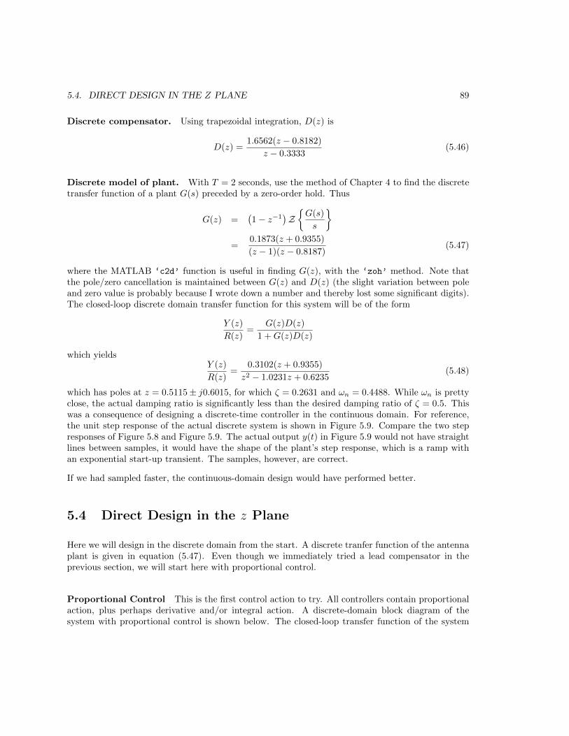
5.4. DIRECT DESIGN IN THE Z PLANE 89
Discrete compensator. Using trapezoidal integration, D(z) is
D(z) =1.6562(z − 0.8182)
z − 0.3333(5.46)
Discrete model of plant. With T = 2 seconds, use the method of Chapter 4 to find the discretetransfer function of a plant G(s) preceded by a zero-order hold. Thus
G(z) =(1− z−1
)ZG(s)
s
=
0.1873(z + 0.9355)
(z − 1)(z − 0.8187)(5.47)
where the MATLAB ‘c2d’ function is useful in finding G(z), with the ‘zoh’ method. Note thatthe pole/zero cancellation is maintained between G(z) and D(z) (the slight variation between poleand zero value is probably because I wrote down a number and thereby lost some significant digits).The closed-loop discrete domain transfer function for this system will be of the form
Y (z)
R(z)=
G(z)D(z)
1 +G(z)D(z)
which yieldsY (z)
R(z)=
0.3102(z + 0.9355)
z2 − 1.0231z + 0.6235(5.48)
which has poles at z = 0.5115± j0.6015, for which ζ = 0.2631 and ωn = 0.4488. While ωn is prettyclose, the actual damping ratio is significantly less than the desired damping ratio of ζ = 0.5. Thiswas a consequence of designing a discrete-time controller in the continuous domain. For reference,the unit step response of the actual discrete system is shown in Figure 5.9. Compare the two stepresponses of Figure 5.8 and Figure 5.9. The actual output y(t) in Figure 5.9 would not have straightlines between samples, it would have the shape of the plant’s step response, which is a ramp withan exponential start-up transient. The samples, however, are correct.
If we had sampled faster, the continuous-domain design would have performed better.
5.4 Direct Design in the z Plane
Here we will design in the discrete domain from the start. A discrete tranfer function of the antennaplant is given in equation (5.47). Even though we immediately tried a lead compensator in theprevious section, we will start here with proportional control.
Proportional Control This is the first control action to try. All controllers contain proportionalaction, plus perhaps derivative and/or integral action. A discrete-domain block diagram of thesystem with proportional control is shown below. The closed-loop transfer function of the system
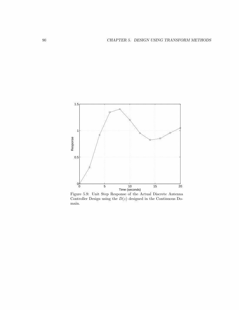
90 CHAPTER 5. DESIGN USING TRANSFORM METHODS
0 5 10 15 200
0.5
1
1.5
Time (seconds)
Res
pons
e
Figure 5.9: Unit Step Response of the Actual Discrete AntennaController Design using the D(z) designed in the Continuous Do-main.
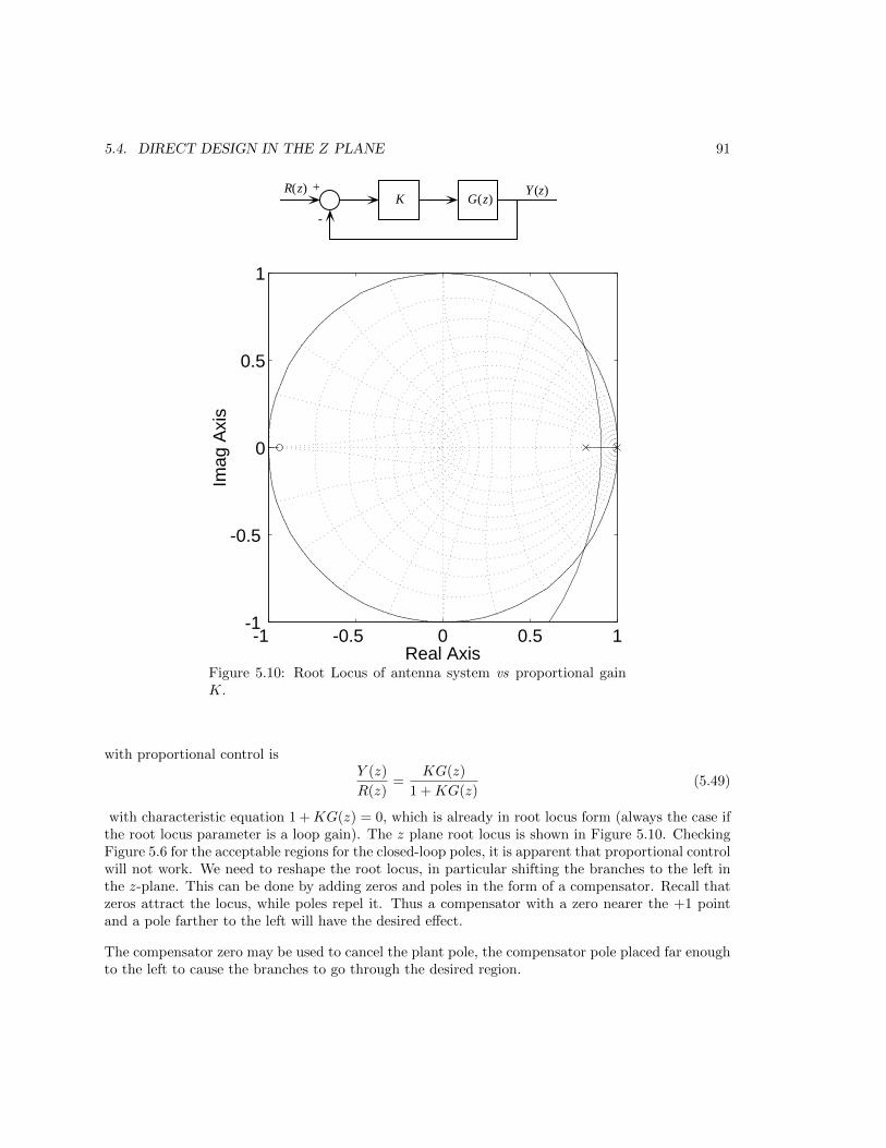
5.4. DIRECT DESIGN IN THE Z PLANE 91
+
-
R(z) Y (z)K G(z)
-1 -0.5 0 0.5 1-1
-0.5
0
0.5
1
Real Axis
Imag
Axi
s
Figure 5.10: Root Locus of antenna system vs proportional gainK.
with proportional control isY (z)
R(z)=
KG(z)
1 +KG(z)(5.49)
with characteristic equation 1 +KG(z) = 0, which is already in root locus form (always the case ifthe root locus parameter is a loop gain). The z plane root locus is shown in Figure 5.10. CheckingFigure 5.6 for the acceptable regions for the closed-loop poles, it is apparent that proportional controlwill not work. We need to reshape the root locus, in particular shifting the branches to the left inthe z-plane. This can be done by adding zeros and poles in the form of a compensator. Recall thatzeros attract the locus, while poles repel it. Thus a compensator with a zero nearer the +1 pointand a pole farther to the left will have the desired effect.
The compensator zero may be used to cancel the plant pole, the compensator pole placed far enoughto the left to cause the branches to go through the desired region.
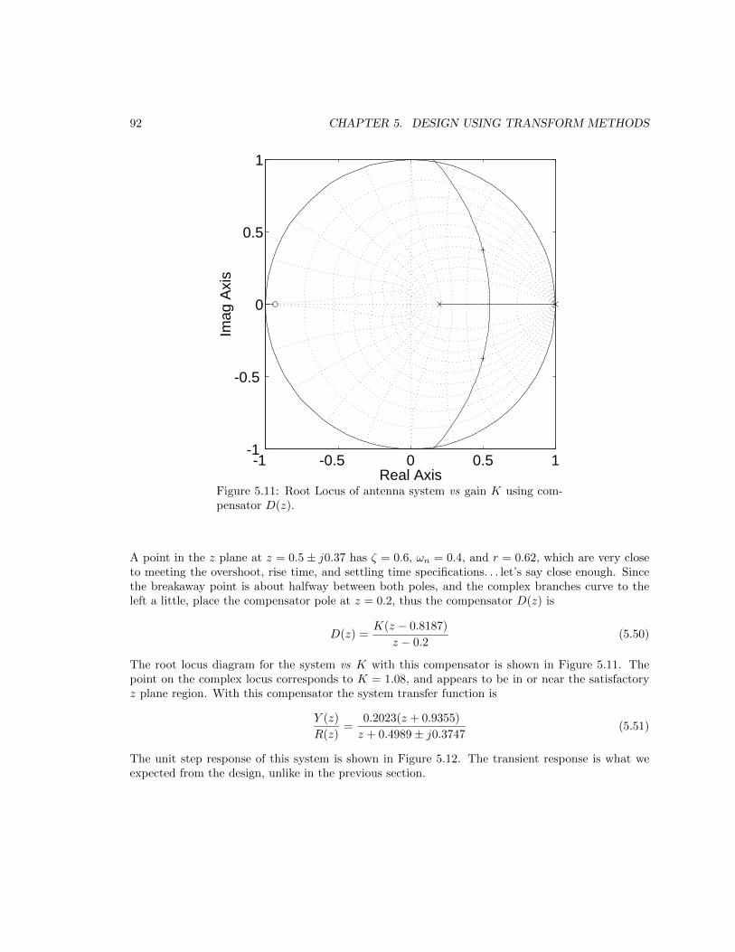
92 CHAPTER 5. DESIGN USING TRANSFORM METHODS
-1 -0.5 0 0.5 1-1
-0.5
0
0.5
1
Real Axis
Imag
Axi
s
Figure 5.11: Root Locus of antenna system vs gain K using com-pensator D(z).
A point in the z plane at z = 0.5± j0.37 has ζ = 0.6, ωn = 0.4, and r = 0.62, which are very closeto meeting the overshoot, rise time, and settling time specifications. . . let’s say close enough. Sincethe breakaway point is about halfway between both poles, and the complex branches curve to theleft a little, place the compensator pole at z = 0.2, thus the compensator D(z) is
D(z) =K(z − 0.8187)
z − 0.2(5.50)
The root locus diagram for the system vs K with this compensator is shown in Figure 5.11. Thepoint on the complex locus corresponds to K = 1.08, and appears to be in or near the satisfactoryz plane region. With this compensator the system transfer function is
Y (z)
R(z)=
0.2023(z + 0.9355)
z + 0.4989± j0.3747(5.51)
The unit step response of this system is shown in Figure 5.12. The transient response is what weexpected from the design, unlike in the previous section.

5.4. DIRECT DESIGN IN THE Z PLANE 93
0 5 10 15 200
0.2
0.4
0.6
0.8
1
1.2
Time (seconds)
Res
pons
e
Figure 5.12: Step response of system designed in z plane.
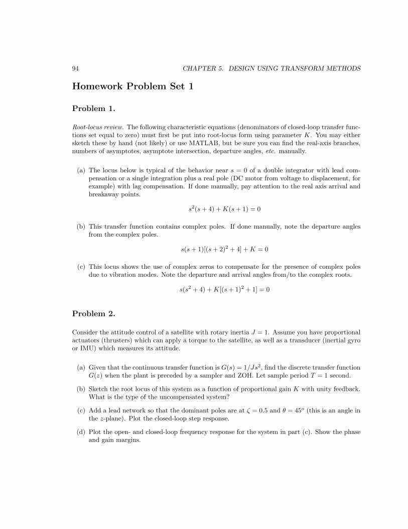
94 CHAPTER 5. DESIGN USING TRANSFORM METHODS
Homework Problem Set 1
Problem 1.
Root-locus review. The following characteristic equations (denominators of closed-loop transfer func-tions set equal to zero) must first be put into root-locus form using parameter K. You may eithersketch these by hand (not likely) or use MATLAB, but be sure you can find the real-axis branches,numbers of asymptotes, asymptote intersection, departure angles, etc. manually.
(a) The locus below is typical of the behavior near s = 0 of a double integrator with lead com-pensation or a single integration plus a real pole (DC motor from voltage to displacement, forexample) with lag compensation. If done manually, pay attention to the real axis arrival andbreakaway points.
s2(s+ 4) +K(s+ 1) = 0
(b) This transfer function contains complex poles. If done manually, note the departure anglesfrom the complex poles.
s(s+ 1)[(s+ 2)2 + 4] +K = 0
(c) This locus shows the use of complex zeros to compensate for the presence of complex polesdue to vibration modes. Note the departure and arrival angles from/to the complex roots.
s(s2 + 4) +K[(s+ 1)2 + 1] = 0
Problem 2.
Consider the attitude control of a satellite with rotary inertia J = 1. Assume you have proportionalactuators (thrusters) which can apply a torque to the satellite, as well as a transducer (inertial gyroor IMU) which measures its attitude.
(a) Given that the continuous transfer function is G(s) = 1/Js2, find the discrete transfer functionG(z) when the plant is preceded by a sampler and ZOH. Let sample period T = 1 second.
(b) Sketch the root locus of this system as a function of proportional gain K with unity feedback.What is the type of the uncompensated system?
(c) Add a lead network so that the dominant poles are at ζ = 0.5 and θ = 45o (this is an angle inthe z-plane). Plot the closed-loop step response.
(d) Plot the open- and closed-loop frequency response for the system in part (c). Show the phaseand gain margins.

5.5. ANOTHER DESIGN EXAMPLE 95
0 0.1 0.2 0.3 0.4 0.50
0.2
0.4
0.6
0.8
1
1.2
1.4
1.6
1.8
Time (seconds)
Pla
nt u
nit s
tep
resp
onse
Figure 5.13: Unit step response of plant G(s).
5.5 Another Design Example
Consider the second-order plant with ζ = 0.1 and ωn = 100 rad/sec (fn ≈ 16 Hz):
G(s) =Y (s)
U(s)=
1002
s2 + 2(0.1)(100)s+ 1002
=10000
s2 + 20s+ 10000(5.52)
This behavior would be encountered when trying to position an inertia through a transmission(shaft, gears, etc.) which has flexibility. The unit step response of this plant may be obtained bythe following MATLAB script:
>>zeta = 0.1;
>>wn = 100;
>>num = [0 0 wn^2];
>>den = [1 2*zeta*wn wn^2];
>>step(num,den);
A plot of the response is shown in Figure 5.13. The slow-decaying oscillation, or “ringing,” isapparent from the plot. Also, the plant G(s) has no free integrations, and therefore will be Type 0.We propose to use a digital feedback control system to meet three performance criteria—

96 CHAPTER 5. DESIGN USING TRANSFORM METHODS
1. Increase damping so that PO <10%.
2. Achieve rise time of tr =0.03 seconds (a little slower than the original plant).
3. Increase system Type to 1.
Note that we have not tried to maintain the rise time of the original system. It might be unrealisticto try to ask for too much, we are already attempting to improve both transient response and andsteady-state error. . . trying to maintain the original speed of response may well be impossible!
Acceptable z-plane regions for poles The first step will be to find translate the transientresponse performance specifications into allowable regions in the z plane. The overshoot and risetime give:
• Overshoot: PO <10% ⇒ ζ > 0.54.
• Rise time: tr < 0.03 seconds ⇒ ωn >1.80.03 = 60 rad/sec.
Sampling rate. To find the acceptable contours in the z plane, we must select a sample periodT (needed to map z = esT . A rule of thumb is to pick the sampling frequency 6 to 20 times greaterthan the highest frequency in the system. The natural frequency of the plant G(s) is about 16 Hz.,so select fs = 100 Hz as the sampling frequency, hence T = 0.01 seconds. This is on the slow side,especially if high-frequency disturbances are expected, but will yield satisfactory results for setpointtracking. The z-plane regions corresponding to the limits on ζ and ωn are shown in Figure 5.14.This figure was generated with the following MATLAB commands:
>>T = 0.01;
>>zeta = 0.54;
>>wn = 60;
>>zgrid(zeta,wn*T,’new’);
>>grid;
>>axis(’square’);
>>axis(’equal’);
Block diagram of control system. A block diagram of the feedback control system is shown inFigure 5.14. As before, assume an error-sampled system, with a D/A converter following the digitalcontroller. A unity feedback loop completes the system.
Discrete model of plant. Preceding the plant G(s) by a sampler and following it with a ZOHyields a discrete plant model G(z). The following MATLAB script (entered interactively) will dothis:
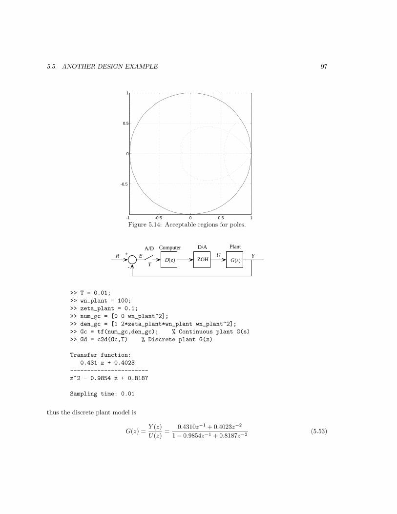
5.5. ANOTHER DESIGN EXAMPLE 97
-1 -0.5 0 0.5 1
-0.5
0
0.5
1
Figure 5.14: Acceptable regions for poles.
A/D Computer D/A Plant
R E U Y
TD(z) G(s)ZOH
+
-
>> T = 0.01;
>> wn_plant = 100;
>> zeta_plant = 0.1;
>> num_gc = [0 0 wn_plant^2];
>> den_gc = [1 2*zeta_plant*wn_plant wn_plant^2];
>> Gc = tf(num_gc,den_gc); % Continuous plant G(s)
>> Gd = c2d(Gc,T) % Discrete plant G(z)
Transfer function:
0.431 z + 0.4023
-----------------------
z^2 - 0.9854 z + 0.8187
Sampling time: 0.01
thus the discrete plant model is
G(z) =Y (z)
U(z)=
0.4310z−1 + 0.4023z−2
1− 0.9854z−1 + 0.8187z−2(5.53)
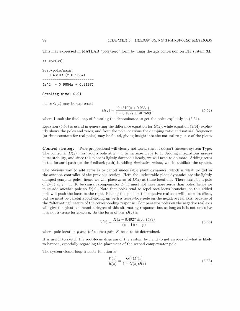
98 CHAPTER 5. DESIGN USING TRANSFORM METHODS
This may expressed in MATLAB “pole/zero” form by using the zpk conversion on LTI system Gd:
>> zpk(Gd)
Zero/pole/gain:
0.43103 (z+0.9334)
-------------------------
(z^2 - 0.9854z + 0.8187)
Sampling time: 0.01
hence G(z) may be expressed
G(z) =0.4310(z + 0.9334)
z − 0.4927± j0.7589, (5.54)
where I took the final step of factoring the denominator to get the poles explicitly in (5.54).
Equation (5.53) is useful in generating the difference equation for G(z), while equation (5.54) explic-itly shows the poles and zeros, and from the pole locations the damping ratio and natural frequency(or time constant for real poles) may be found, giving insight into the natural response of the plant.
Control strategy. Pure proportional will clearly not work, since it doesn’t increase system Type.The controller D(z) must add a pole at z = 1 to increase Type to 1. Adding integrations alwayshurts stability, and since this plant is lightly damped already, we will need to do more. Adding zerosin the forward path (or the feedback path) is adding derivative action, which stabilizes the system.
The obvious way to add zeros is to cancel undesirable plant dynamics, which is what we did inthe antenna controller of the previous section. Here the undesirable plant dynamics are the lightlydamped complex poles, hence we will place zeros of D(z) at these locations. There must be a poleof D(z) at z = 1. To be causal, compensator D(z) must not have more zeros than poles, hence wemust add another pole to D(z). Note that poles tend to repel root locus branches, so this addedpole will push the locus to the right. Placing this pole on the negative real axis will lessen its effect,but we must be careful about ending up with a closed-loop pole on the negative real axis, because ofthe “alternating” nature of the corresponding response. Compensator poles on the negative real axiswill give the plant command a degree of this alternating response, but as long as it is not excessiveit is not a cause for concern. So the form of our D(z) is
D(z) =K(z − 0.4927± j0.7589)
(z − 1)(z − p)(5.55)
where pole location p and (of course) gain K need to be determined.
It is useful to sketch the root-locus diagram of the system by hand to get an idea of what is likelyto happen, especially regarding the placement of the second compensator pole.
The system closed-loop transfer function is
Y (z)
R(z)=
G(z)D(z)
1 +G(z)D(z)(5.56)

5.5. ANOTHER DESIGN EXAMPLE 99
-1 -0.5 0 0.5 1-1
-0.8
-0.6
-0.4
-0.2
0
0.2
0.4
0.6
0.8
1
Real
Imag
Figure 5.15: Hand sketch of root locus for Example 2.
and the system characteristic equation is
1 +G(z)D(z) = 0 (5.57)
which upon substitution for G(z) and D(z) becomes
1 +0.4310K(z − 0.4927± j0.7589)(z + 0.9334)
(z − 0.4927± j0.7589)(z − 1)(z − p)(5.58)
The complex poles and zeros may be algebraically cancelled, leaving
1 +0.4310K(z + 0.9334)
(z − 1)(z − p)(5.59)
A hand sketch of this locus for p = 0 is shown in Figure 5.15. The canceled pole and zero are notshown in Figure 5.15, this simplifies the sketch.
Computer root locus analysis. Comparing the hand-drawn sketch of Figure 5.15 with theregion of acceptibility in Figure 5.14, it looks like placing the second pole of D(z) at z = 0 maywork. A root locus diagram may be generated using MATLAB as follows:
>>num_rl = 0.4310*[1 0.9334];
>>den_rl = conv([1 -1],[1 0]);
>>zgrid(’new’);
>>rlocus(num_rl,den_rl);

100 CHAPTER 5. DESIGN USING TRANSFORM METHODS
-1 -0.5 0 0.5 1-1
-0.5
0
0.5
1
Real Axis
Imag
Axi
s
Figure 5.16: MATLAB root locus for Example 2.
The zgrid(‘new’) function draws a z-plane, with lines of constant damping ratio (ζ = 0.1, 0.2, 0.3, . . ., 0.8, 0.9),and lines of constant natural frequency (ωnT = 0.1π, 0.2π, . . ., 0.8π, 0.9π). These lines aid selectionof desired pole locations, which is done using the rlocfind function as shown below, where I haveselected a damping ratio of ζ = 0.7.
>>K = rlocfind(num_rl,den_rl);
Select a point in the graphics window
selected_point =
0.3707 + 0.3245i
>>K
K =
0.6022
The selected closed-loop pole locations are shown by a “star” on the root locus of Figure 5.16.
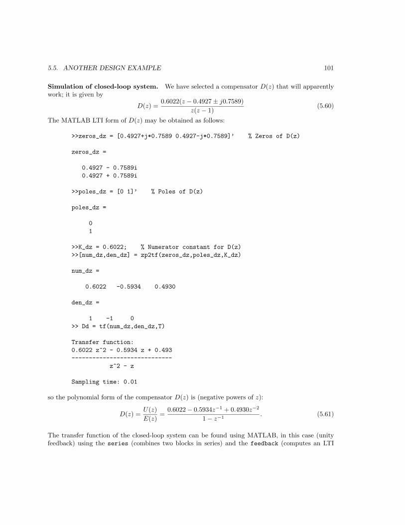
5.5. ANOTHER DESIGN EXAMPLE 101
Simulation of closed-loop system. We have selected a compensator D(z) that will apparentlywork; it is given by
D(z) =0.6022(z − 0.4927± j0.7589)
z(z − 1)(5.60)
The MATLAB LTI form of D(z) may be obtained as follows:
>>zeros_dz = [0.4927+j*0.7589 0.4927-j*0.7589]’ % Zeros of D(z)
zeros_dz =
0.4927 - 0.7589i
0.4927 + 0.7589i
>>poles_dz = [0 1]’ % Poles of D(z)
poles_dz =
0
1
>>K_dz = 0.6022; % Numerator constant for D(z)
>>[num_dz,den_dz] = zp2tf(zeros_dz,poles_dz,K_dz)
num_dz =
0.6022 -0.5934 0.4930
den_dz =
1 -1 0
>> Dd = tf(num_dz,den_dz,T)
Transfer function:
0.6022 z^2 - 0.5934 z + 0.493
-----------------------------
z^2 - z
Sampling time: 0.01
so the polynomial form of the compensator D(z) is (negative powers of z):
D(z) =U(z)
E(z)=
0.6022− 0.5934z−1 + 0.4930z−2
1− z−1. (5.61)
The transfer function of the closed-loop system can be found using MATLAB, in this case (unityfeedback) using the series (combines two blocks in series) and the feedback (computes an LTI

102 CHAPTER 5. DESIGN USING TRANSFORM METHODS
0 0.02 0.04 0.06 0.08 0.10
0.2
0.4
0.6
0.8
1
1.2
Time(seconds)
Res
pons
e y(
t)
Unit Step Response
Figure 5.17: Unit step response of closed-loop system for Example 2.
model for a feedback loop) functions. We have both D(z) and G(z) in MATLAB LTI form, so:
>> forward = series(Dd,Gd); % Forward path is D(z)*G(z)
>> sys_cl = feedback(forward,1); % Closed-loop, unity feedback
Note that MATLAB will not do pole/zero cancellation (look at sys cl in MATLAB, for example),but they will cancel numerically during a response simulation.
Step response. The unit step response of the closed-loop system is shown in Figure 5.17. Comparethis plot with the uncontrolled plant of Figure 5.13. The MATLAB commands that generated thisresponse are
>>k = 0:10; % Define sample sequence
>>t = k*T; % Define time vector
>>y = step(sys_cl,t); % Generate samples corresponding to time vector
>>plot(t,y,’o’,t,y,’-’);
>>grid;
>>xlabel(’Time(seconds)’);
>>ylabel(’Response y(t)’);
>>title(’Unit Step Response’);
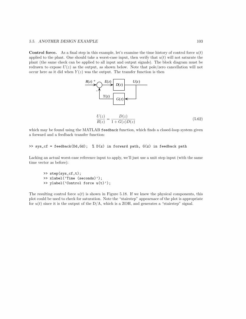
5.5. ANOTHER DESIGN EXAMPLE 103
Control force. As a final step in this example, let’s examine the time history of control force u(t)applied to the plant. One should take a worst-case input, then verify that u(t) will not saturate theplant (the same check can be applied to all input and output signals). The block diagram must beredrawn to expose U(z) as the output, as shown below. Note that pole/zero cancellation will notoccur here as it did when Y (z) was the output. The transfer function is then
+
-
R(z) E(z) U(z )
Y (z)
D(z)
G(z)
U(z)
R(z)=
D(z)
1 +G(z)D(z)(5.62)
which may be found using the MATLAB feedback function, which finds a closed-loop system givena forward and a feedback transfer function:
>> sys_cf = feedback(Dd,Gd); % D(z) in forward path, G(z) in feedback path
Lacking an actual worst-case reference input to apply, we’ll just use a unit step input (with the sametime vector as before):
>> step(sys_cf,t);
>> xlabel(’Time (seconds)’);
>> ylabel(’Control force u(t)’);
The resulting control force u(t) is shown in Figure 5.18. If we knew the physical components, thisplot could be used to check for saturation. Note the “stairstep” appearnace of the plot is appropriatefor u(t) since it is the output of the D/A, which is a ZOH, and generates a “stairstep” signal.

104 CHAPTER 5. DESIGN USING TRANSFORM METHODS
0 0.01 0.02 0.03 0.04 0.05 0.06 0.07 0.08 0.09 0.10.4
0.5
0.6
0.7
0.8
0.9
1
1.1
Time (seconds)
Con
trol
forc
e u(
t)
Figure 5.18: Control force u(t) for unit step r(t) in Example 2.
5.6 Modeling using Simulink
The MATLAB “companion” application Simulink offers a graphical approach to system simulation,and is frequently more useful than “plain MATLAB” for that function. However, it is the author’sopinion that a good grounding in MATLAB must precede the use of Simulink. Also,
“Simulink is only for simulation, and is NOT A DESIGN TOOL!!”
That being said, we’ll use the design example of Section 5.5 as the system to illustrate the use ofSimulink. Refer now to the block diagram of Figure 5.14, which is reproduced in Figure 5.19.
Recall that the compensator D(z) transfer function in Figure 5.19 is given by
D(z) =0.6022z2 − 0.5943z + 0.493
z(z − 1)=
0.6022z2 − 0.5943z + 0.493
z2 − z(5.63)
The steps in creating a Simulink model of this system will be described below.

5.6. MODELING USING SIMULINK 105
D(z)1002
s2 + 2(0.1)(100)s + 1002
ZOH
+
!
R(s) E(s) E(z) U(s) Y (s)compensator second-order plant G(s)
T
Figure 5.19: Block diagram for Simulink model.
5.6.1 Creating the Simulink Model
Figure 5.20 below shows the finished model. Note that it bears a very strong resemblance to theblock diagram of Figure 5.19.
Zero−OrderHold
10000s +20s+100002
Transfer FcnStep Output y
0.6022z −0.5934z+0.4932
z −z2
DiscreteTransfer Fcn
Control u
e ury
y
Figure 5.20: Block diagram of the finished Simulink model.
The blocks I used in creating this model are: Sum, Discrete Transfer Fcn, Zero-Order Hold,
Transfer Fcn, Step, Scope. I didn’t change their names in Figure 5.20 for clarity (except for thescopes). After placing a block you may change its name to reflect its physical significance.
Some items of note are:
• I modified step to occur at t = 0 instead of the t = 1 default.
• In placing the Discrete Transfer Fcn a sampler is automatically created. You must specifythe sample period (T = 0.01 here) while modifying the block.
• The Zero-Order Hold block can “inherit” its sample period (-1 for sample time).
• Double-click on a signal path to enter a name (like r, e, u, y).
• The “stop time” under Simulation/Configuration Parameters should be changed from itsdefault of 10 seconds to 0.1 seconds.
One of the advantageous of using Simulink is that “intermediate” variables (like control force u)can be easily displaced by just “picking them off” and connecting to a scope. The Simulink plot-ting facilities are minimal, but a given variable can be connected to a “to Workspace” block forsubsequent plotting in MATLAB.
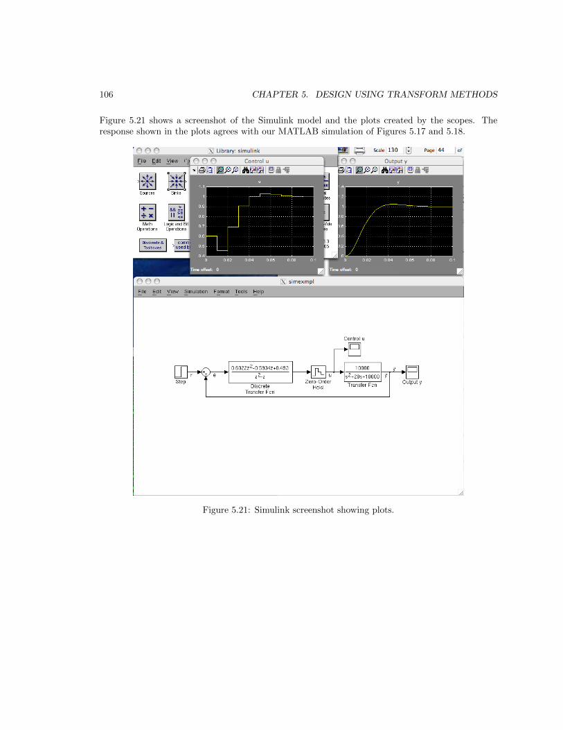
106 CHAPTER 5. DESIGN USING TRANSFORM METHODS
Figure 5.21 shows a screenshot of the Simulink model and the plots created by the scopes. Theresponse shown in the plots agrees with our MATLAB simulation of Figures 5.17 and 5.18.
Figure 5.21: Simulink screenshot showing plots.

5.7. PID CONTROL (MODE CONTROLLERS) 107
5.7 PID Control (Mode Controllers)
There are three basic types of control actions:
• Proportional—control force is proportional to the error signal.
• Integral—control force is proportional to the integral of the error signal
• Derivative—control force is proportional to the derivative of the error signal.
Integral and derivative control actions are used in combination with proportional, hence PI, PD, orPID controllers. The control modes are used in parallel, as shown in the block diagram of Figure 5.22.PID control action in the continuous domain is given by
++
+
e( t) u(t)KDs
KP
KI
s
Figure 5.22: PID control action
u(t) = KP e(t) +KI
∫ t
0
e(t)dt+KD e(t). (5.64)
The three control actions will now be considered in the discrete domain.
5.7.1 Proportional Control
A discrete implementation of proportional control action is identical to continuous, thus
u(t) = KP e(t)⇒ D(s) = KP ,
the discrete is
uk = KP ek ⇒ D(z) = KP
Proportional control is always present—either by itself, or allied with derivative and/or integralcontrol as shown below.
108 CHAPTER 5. DESIGN USING TRANSFORM METHODS
5.7.2 Derivative Action
In continuous systems, derivative action has the form
u(t) = KD e(t)⇒ D(s) = KDs.
In the discrete domain, differentiation can be approximated by the first difference, that is,
uk = KDek − ek−1 ⇒ D(z) = KD(1− z−1) = KDz − 1
z
Derivative action is typically used to improve system stability and transient response.
5.7.3 Integral Action
Continuous integral action is given by
u(t) = KI
∫ t
0
e(t)dt⇒ D(s) =KI
s
Discrete integration is a cumulative sum, represented by
uk = uk−1 +KIek ⇒ D(z) = KI1
1− z−1= KI
z
z − 1
NOTE: Gains KI and KD have different values in the continuous and discrete domains!
Integral action is typically used to improve system steady-state error behavior. It usually worsenstransient response and stability.
The I and D control actions are rarely used by themselves, but are coupled with proportional (P)action for PD, PI, or PID controllers.
5.7.4 PD Control
The combination of Proportional and Derivative action is given by
KP +KDz − 1
z=
KD
(z − KD+KP
KD
)z
=K(z − a)
z
which is a lead compensator of the same form we used in Example 2.
5.7. PID CONTROL (MODE CONTROLLERS) 109
5.7.5 PI Control
Proportional plus Integral control is
KP +KIz
z − 1=
(KP +KI)(z − KP
KP+KI
)z − 1
=K(z − a)
z − 1
which has a pole at z = 1 corresponding to the integration, and a zero on the positive real axisnearer the origin. It is this pole at z = 1 that improves steady-state behavior but hurts stabilityand transient response. The zero is usually placed fairly near the pole at z = 1 to reduce the effectof the “slow” closed-loop pole that will be in this region. Note that it is the open-loop pole at z = 1that improves the steady-state error by raising the Type (see Sec. 5.2.1) of the system.
5.7.6 PID Control
Adding integral action to form three-mode proportional plus integral plus derivative action yields
KP +KDz − 1
z+KI
z
z − 1=
(KP +KD +KI) z2 − (KP + 2KD) z +KD
z(z − 1)
=K(z2 − az + b)
z(z − 1)
which has a pole at z = 1 from the integration, a pole at z = 0, and two zeros which may be real orcomplex, depending on the relative values of the three gains.
One strategy for PID design is as follows:
1. Place one zero and pole as for the PD design.
2. Place the second pole at z = 1 (the integration), and place the zero “nearby” for the samereason discussed at the end of Section 5.7.5 above.
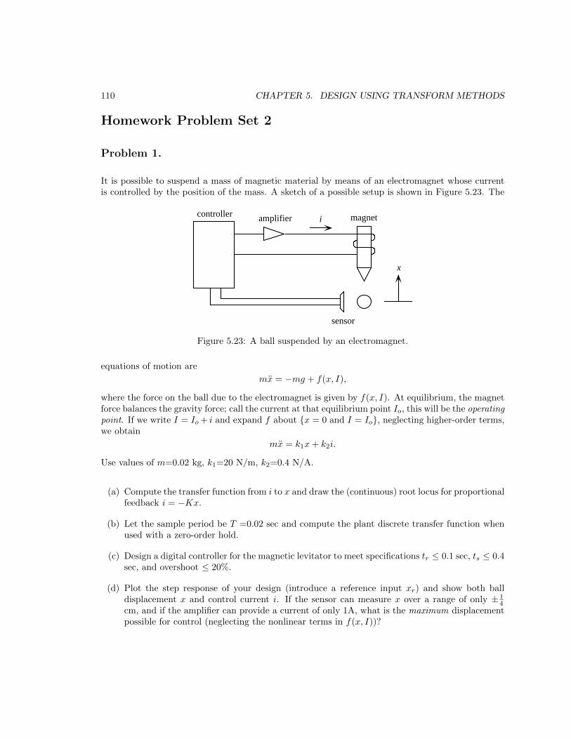
110 CHAPTER 5. DESIGN USING TRANSFORM METHODS
Homework Problem Set 2
Problem 1.
It is possible to suspend a mass of magnetic material by means of an electromagnet whose currentis controlled by the position of the mass. A sketch of a possible setup is shown in Figure 5.23. The
controller amplifier magnet
sensor
x
i
Figure 5.23: A ball suspended by an electromagnet.
equations of motion are
mx = −mg + f(x, I),
where the force on the ball due to the electromagnet is given by f(x, I). At equilibrium, the magnetforce balances the gravity force; call the current at that equilibrium point Io, this will be the operatingpoint. If we write I = Io + i and expand f about x = 0 and I = Io, neglecting higher-order terms,we obtain
mx = k1x+ k2i.
Use values of m=0.02 kg, k1=20 N/m, k2=0.4 N/A.
(a) Compute the transfer function from i to x and draw the (continuous) root locus for proportionalfeedback i = −Kx.
(b) Let the sample period be T =0.02 sec and compute the plant discrete transfer function whenused with a zero-order hold.
(c) Design a digital controller for the magnetic levitator to meet specifications tr ≤ 0.1 sec, ts ≤ 0.4sec, and overshoot ≤ 20%.
(d) Plot the step response of your design (introduce a reference input xr) and show both balldisplacement x and control current i. If the sensor can measure x over a range of only ± 1
4cm, and if the amplifier can provide a current of only 1A, what is the maximum displacementpossible for control (neglecting the nonlinear terms in f(x, I))?
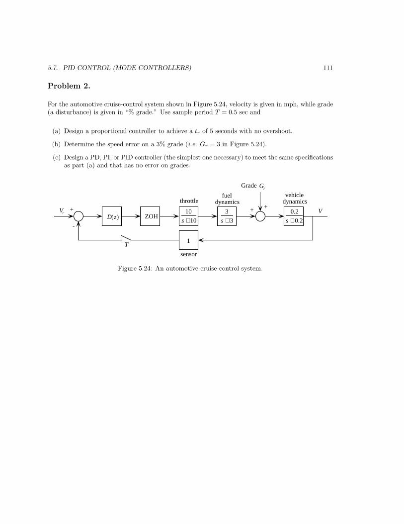
5.7. PID CONTROL (MODE CONTROLLERS) 111
Problem 2.
For the automotive cruise-control system shown in Figure 5.24, velocity is given in mph, while grade(a disturbance) is given in “% grade.” Use sample period T = 0.5 sec and
(a) Design a proportional controller to achieve a tr of 5 seconds with no overshoot.
(b) Determine the speed error on a 3% grade (i.e. Gr = 3 in Figure 5.24).
(c) Design a PD, PI, or PID controller (the simplest one necessary) to meet the same specificationsas part (a) and that has no error on grades.
ZOH
throttlefuel
dynamicsvehicle
dynamics
sensor
Grade
Vr+
-
+ +
T
V
1
D(z)10
s +10
3
s + 3
0.2
s + 0.2
Gr
Figure 5.24: An automotive cruise-control system.

112 CHAPTER 5. DESIGN USING TRANSFORM METHODS
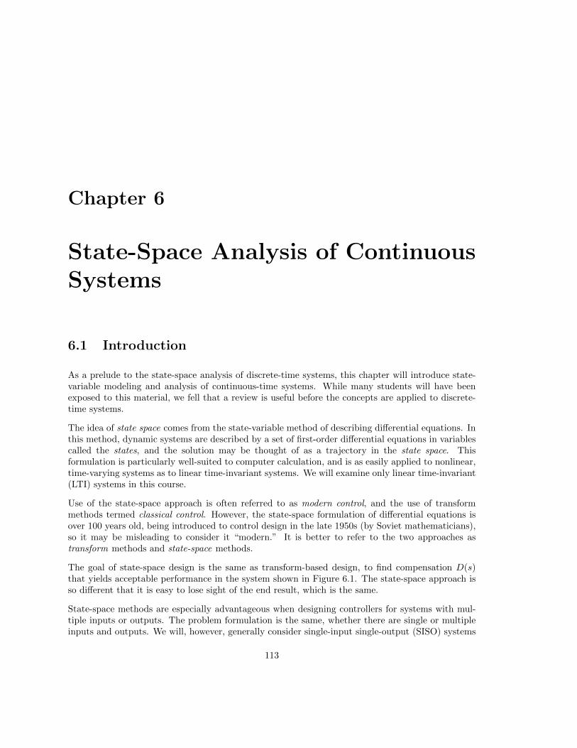
Chapter 6
State-Space Analysis of ContinuousSystems
6.1 Introduction
As a prelude to the state-space analysis of discrete-time systems, this chapter will introduce state-variable modeling and analysis of continuous-time systems. While many students will have beenexposed to this material, we fell that a review is useful before the concepts are applied to discrete-time systems.
The idea of state space comes from the state-variable method of describing differential equations. Inthis method, dynamic systems are described by a set of first-order differential equations in variablescalled the states, and the solution may be thought of as a trajectory in the state space. Thisformulation is particularly well-suited to computer calculation, and is as easily applied to nonlinear,time-varying systems as to linear time-invariant systems. We will examine only linear time-invariant(LTI) systems in this course.
Use of the state-space approach is often referred to as modern control, and the use of transformmethods termed classical control. However, the state-space formulation of differential equations isover 100 years old, being introduced to control design in the late 1950s (by Soviet mathematicians),so it may be misleading to consider it “modern.” It is better to refer to the two approaches astransform methods and state-space methods.
The goal of state-space design is the same as transform-based design, to find compensation D(s)that yields acceptable performance in the system shown in Figure 6.1. The state-space approach isso different that it is easy to lose sight of the end result, which is the same.
State-space methods are especially advantageous when designing controllers for systems with mul-tiple inputs or outputs. The problem formulation is the same, whether there are single or multipleinputs and outputs. We will, however, generally consider single-input single-output (SISO) systems
113
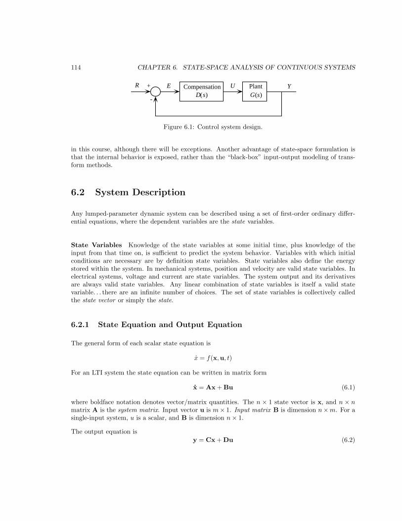
114 CHAPTER 6. STATE-SPACE ANALYSIS OF CONTINUOUS SYSTEMS
Compensation PlantR E U Y+
-D(s) G(s)
Figure 6.1: Control system design.
in this course, although there will be exceptions. Another advantage of state-space formulation isthat the internal behavior is exposed, rather than the “black-box” input-output modeling of trans-form methods.
6.2 System Description
Any lumped-parameter dynamic system can be described using a set of first-order ordinary differ-ential equations, where the dependent variables are the state variables.
State Variables Knowledge of the state variables at some initial time, plus knowledge of theinput from that time on, is sufficient to predict the system behavior. Variables with which initialconditions are necessary are by definition state variables. State variables also define the energystored within the system. In mechanical systems, position and velocity are valid state variables. Inelectrical systems, voltage and current are state variables. The system output and its derivativesare always valid state variables. Any linear combination of state variables is itself a valid statevariable. . . there are an infinite number of choices. The set of state variables is collectively calledthe state vector or simply the state.
6.2.1 State Equation and Output Equation
The general form of each scalar state equation is
x = f(x,u, t)
For an LTI system the state equation can be written in matrix form
x = Ax + Bu (6.1)
where boldface notation denotes vector/matrix quantities. The n × 1 state vector is x, and n × nmatrix A is the system matrix. Input vector u is m× 1. Input matrix B is dimension n×m. For asingle-input system, u is a scalar, and B is dimension n× 1.
The output equation is
y = Cx + Du (6.2)
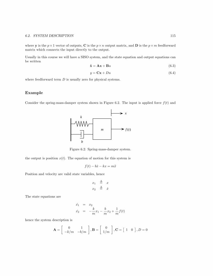
6.2. SYSTEM DESCRIPTION 115
where y is the p×1 vector of outputs, C is the p×n output matrix, and D is the p×m feedforwardmatrix which connects the input directly to the output.
Usually in this course we will have a SISO system, and the state equation and output equations canbe written
x = Ax + Bu (6.3)
y = Cx +Du (6.4)
where feedforward term D is usually zero for physical systems.
Example
Consider the spring-mass-damper system shown in Figure 6.2. The input is applied force f(t) and
k
b
m
x
f (t)
Figure 6.2: Spring-mass-damper system.
the output is position x(t). The equation of motion for this system is
f(t)− bx− kx = mx
Position and velocity are valid state variables, hence
x1∆= x
x2∆= x
The state equations are
x1 = x2
x2 = − kmx1 −
b
mx2 +
1
mf(t)
hence the system description is
A =
[0 1
−k/m −b/m
],B =
[0
1/m
],C =
[1 0
], D = 0
116 CHAPTER 6. STATE-SPACE ANALYSIS OF CONTINUOUS SYSTEMS
6.2.2 State equation from Transfer Function
Given transfer functionY (s)
U(s)=
b2s2 + b1s+ b0
s3 + a2s2 + a1s+ a0(6.5)
it can be shown that a state equation is x1
x2
x3
=
0 1 00 0 1−a0 −a1 −a2
x1
x2
x3
+
001
u(t) (6.6)
and the output equation is
y(t) =[b0 b1 b2
] x1
x2
x3
(6.7)
We will see shortly that equations (6.6–6.7) are in a special (minimal) form called (lower) controlcanonical form.
6.2.3 Transfer Function from State-Variable Description
It is possible to get a transfer function from the state space description of a system. Assuming zeroinitial conditions on state x, taking the Laplace transform of state equation
x = Ax + Bu (6.8)
yieldssX(s) = AX(s) + BU(s) (6.9)
which can be rearranged (paying attention to the multiplication order since these are matrices!) as
(sI−A)X(s) = BU(s) (6.10)
which can be solved forX(s) = (sI−A)
−1BU(s) (6.11)
Output equation y = Cx +Du with D = 0 has Laplace transform
Y (s) = Cx(s) (6.12)
which can be used to getY (s) = C(sI−A)
−1BU(s) (6.13)
from which we get the transfer function as
Y (s)
U(s)= C(sI−A)
−1B (6.14)
6.3. DIFFERENT STATE-SPACE REPRESENTATIONS 117
Example
The transfer function of the spring-mass-damper system is
X(s)
F (s)=
1/m
s2 + (b/m)s+ (k/m)
and if we let m = 1, b = 2, k = 4 we get
X(s)
F (s)=
1
s2 + 2s+ 4
The corresponding state-variable description is
A =
[0 1−4 −2
],B =
[01
],C =
[1 0
], D = 0.
Then
sI−A =
[s −14 s+ 2
]and
(sI−A)−1 =
[s+ 2 1−4 s
]s(s+ 2) + 4
The transfer function is given by
C(sI−A)−1
B =
[1 0
] [ s+ 2 1−4 s
] [01
]s(s+ 2) + 4
which yieldsX(s)
F (s)=
1
s2 + 2s+ 4.
Numerical conversion between state-space form to transfer function form can be easily done withMATLAB, as will be shown later.
6.3 Different State-Space Representations
In Section 6.2 we mentioned that there are an infinite number of choices for system state, andcorresponding system matrices. This section presents some standard representations. First comes theidea of state equation transformations, followed by several different representations. The usefulnessof some of these descriptions may not be immediately apparent. Where we need a specific system,we will consider the third-order transfer function
Y (s)
U(s)=
b2s2 + b1s+ b0
s3 + a2s2 + a1s+ a0=b(s)
a(s)(6.15)

118 CHAPTER 6. STATE-SPACE ANALYSIS OF CONTINUOUS SYSTEMS
6.3.1 State Variable Transformation
Given state equationx = Ax + Bu (6.16)
and output equationy = Cx +Du (6.17)
let a new state vector z be defined byz = Tx (6.18)
where T is a n×n non-singular matrix. Note that T must be invertible to permit mapping betweenboth state vectors, thus
x = T−1z (6.19)
Now, starting with the new state z, we have
z = Tx = TAx + TBu (6.20)
then substituting for x yieldsz = TAT−1z + TBu (6.21)
and the output equation isy = CT−1z +Du. (6.22)
Although eigenvalues and eigenvectors will described in Section 6.3.3, the eigenvalues of originalsystem matrix A and “new” matrix TAT−1 are the same!. For this reason these matrices are called“similar.”
6.3.2 Control Canonical Form
Introduce a variable v which relates polynomials a(s) and b(s) as shown in Figure 6.3(a). Thetransfer function from u to v is
V (s)
U(s)=
1
a(s)=
1
s3 + a2s2 + a1s+ a0(6.23)
or...v +a2v + a1v + a0v = u (6.24)
which may be written...v= −a2v − a1v − a0v + u (6.25)
A block diagram illustrating (6.25) is shown in Figure 6.3(b).
The output y is formed byY (s) = b(s)V (s) (6.26)
which meansy = b2v + b1v + b0v (6.27)
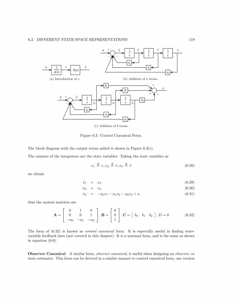
6.3. DIFFERENT STATE-SPACE REPRESENTATIONS 119
u v y1
a(s)b(s)
(a) Introduction of v.
1
s
1
s
1
s
a0
a1
a2
u ˙v ˙v v v
- --
+
(b) Addition of a terms.
1
s
1
s
1
s
a0
a1
a2
u ˙v
- --
+b0
b1
b2+
+ +
y
x3 x2 x1
(c) Addition of b terms.
Figure 6.3: Control Canonical Form.
The block diagram with the output terms added is shown in Figure 6.3(c).
The outputs of the integrators are the state variables. Taking the state variables as
x1∆= v, x2
∆= v, x3
∆= v (6.28)
we obtain
x1 = x2 (6.29)
x2 = x3 (6.30)
x3 = −a0x1 − a1x2 − a2x3 + u (6.31)
thus the system matrices are
A =
0 1 00 0 1−a0 −a1 −a2
,B =
001
,C =[b0 b1 b2
], D = 0 (6.32)
The form of (6.32) is known as control canonical form. It is especially useful in finding state-variable feedback laws (not covered in this chapter). It is a minimal form, and is the same as shownin equation (6.6).
Observer Canonical A similar form, observer canonical, is useful when designing an observer, orstate estimator. This form can be derived in a similar manner to control canonical form, one version
120 CHAPTER 6. STATE-SPACE ANALYSIS OF CONTINUOUS SYSTEMS
of the result is:
A =
−a2 1 0−a1 0 1−a0 0 0
,B =
b2b1b0
,C =[
1 0 0], D = 0. (6.33)
With the observer canonical form the output y = x1.
6.3.3 Diagonal (modal or decoupled) Form
The simplest representation of a state-space system occurs when the state equation are decoupled,that is, when system matrix A is in diagonalized form, in the form
Λ =
λ1
λ2
. . .
λn
(6.34)
Eigenvalues and Eigenvectors Given matrix A, vector x is an eigenvector if
Ax =λx (6.35)
where λ is a scalar eigenvalue. These exceptional vectors get shrunk or reversed by A but theydon’t change direction. The relationship between the state variables stays fixed. Eigenvectors arecommonly called mode shapes, and they represent the natural response modes of the system.
To find the eigenvalues write the equation as (A−λI)x = 0. For this equation to have a non-trivialsolution for x, matrix A− λI must be singular, therefore it must have a zero determinant, and
|A− λI| = 0 (6.36)
This is also the characteristic equation of the system, and poles and eigenvalues are the same thing.An nth order system will (usually) have n eigenvalues λ1. . .λn.
To find the ith eigenvector, solve the system
(A− λiI)xi = 0 (6.37)
for eigenvector xi. MATLAB function eig is used for finding eigenvalues and eigenvectors.
Diagonalization The matrix of eigenvectors are just what we need to diagonalize matrix A. Weneed transformation matrix T such that
Λ = TAT−1
6.4. MATLAB TOOLS 121
Multiply A times the matrix S of its eigenvectors,
AS = A[x1 · · ·xn] = [λ1x1 · · ·λnxn] (6.38)
then write this as
[λ1x1 · · ·λnxn] = [x1 · · ·xn]
λ1
. . .
λn
= SΛ (6.39)
So then we have
AS = SΛ→ Λ = S−1AS (6.40)
Note that by the format of equation (6.21) the diagonalizing transform is T = S−1, where S is thematrix whose columns are the eigenvectors.
The modal form is especially useful in structural dynamics, where there is concern for structuralmode shapes and natural frequencies (square root of eigenvalues). MATLAB function canon() withthe modal option will diagonalize a matrix, and return the transformation T that it used.
6.4 MATLAB Tools
Many MATLAB functions exist for handling state-space systems, some common ones will be de-scribed in this section.
6.4.1 Transform↔State-Space
Changing between transform and state-space domains is done with tf2ss and ss2tf. These workidentically in the continuous and discrete domains.
tf2ss. This function converts a transform-based form to state space representation. The A,B,C,Dmatrices are returned in (upper) control canonical form, slightly different than the (lower) controlcanonical form of Section 6.3.2. A transformation may be used to convert between these forms. Thisis illustrated by the following example. Consider transfer function
G(s) =s2 + 5s+ 6
s3 + 2s2 + 3s+ 4
This may be converted to state-space form by
122 CHAPTER 6. STATE-SPACE ANALYSIS OF CONTINUOUS SYSTEMS
>>num = [0 1 5 6];
>>den = [1 2 3 4];
>>[A,B,C,D] = tf2ss(num,den)
A = -2 -3 -4
1 0 0
0 1 0
B = 1
0
0
C = 1 5 6
D = 0
To transform this to lower canonical form one can use the change of state
z = Tx.
with matrix T given by
>>T = flipud(eye(3))
T = 0 0 1
0 1 0
1 0 0
It is easily seen that T simply reverses the order of the state variables. To transform the state-spacemodel use the ss2ss function:
>>[Al,Bl,Cl,Dl] = ss2ss(A,B,C,D,T)
Al = 0 1 0
0 0 1
-4 -3 -2
Bl = 0
0
1
Cl = 6 5 1
Dl = 0
where the state-space is now in the format of equation (6.32).
6.4. MATLAB TOOLS 123
ss2tf. This just goes the other way. For the previous example, using either canonical form (allstate-space forms must yield the same input-output model):
>>[num,den] = ss2tf(A,B,C,D)
num = 0 1.0000 5.0000 6.0000
den = 1.0000 2.0000 3.0000 4.0000
6.4.2 Eigenvalues, Eigenvectors, Diagonalization
Matlab function eig finds the eigenvalues and eigenvectors. The eigenvectors will be different de-pending on the form of the state equations, but the eigenvalues will always be the same. Consideringthe previous example, using the lower canonical form
>>[Vectors,Values] = eig(Al)
Vectors = 0.2995 -0.1781 - 0.2754i -0.1781 + 0.2754i
-0.4944 0.4572 - 0.2274i 0.4572 + 0.2274i
0.8160 0.2718 + 0.7469i 0.2718 - 0.7469i
Values = -1.6506 0 0
0 -0.1747 + 1.5469i 0
0 0 -0.1747 - 1.5469i
Function eig returns a matrix whose columns are the eigenvectors, and a matrix whose diagonalelements are the eigenvalues. For a system matrix with real coefficients the eigenvalues will alwaysbe either real or complex conjugate pairs. The eigenvalues are the roots of the denominator of theoriginal G(s).
We showed that the transformation needed to diagonalize the system matrix was the inverse of theeigenvector matrix. To verify this,
>>Tdiag = inv(Vectors)
Tdiag = 1.7700 - 0.0000i 0.2552 - 0.0000i 0.7304 - 0.0000i
0.4032 + 1.1137i 0.9842 + 0.4976i 0.4483 - 0.1073i
0.4032 - 1.1137i 0.9842 - 0.4976i 0.4483 + 0.1073i
Now use transformation Tdiag to change state using ss2ss:

124 CHAPTER 6. STATE-SPACE ANALYSIS OF CONTINUOUS SYSTEMS
>>[Ad,Bd,Cd,Dd] = ss2ss(Al,Bl,Cl,Dl,Tdiag)
Ad = -1.6506 - 0.0000i 0.0000 + 0.0000i 0.0000 - 0.0000i
0.0000 + 0.0000i -0.1747 + 1.5469i 0.0000 - 0.0000i
0.0000 - 0.0000i 0.0000 + 0.0000i -0.1747 - 1.5469i
Bd = 0.7304 - 0.0000i
0.4483 - 0.1073i
0.4483 + 0.1073i
Cd = 0.1412 + 0.0000i 1.4891 - 2.0425i 1.4891 + 2.0425i
Dd = 0
canon. MATLAB function canon transforms the state equations into a modal “canonical” form inwhich the real eigenvalues appear on the diagonal, and complex eigenvalues appear in a 2× 2 blockon the diagonal of the A matrix. For a system with eigenvalues λ1, σ ± jω, the modal A matrix is
A =
λ1 0 00 σ ω0 −ω σ
For the original A,B,C,D system,
>>[Am,Bm,Cm,Dm,Tmodal] = canon(A,B,C,D,’modal’)
Am = -1.6506 0.0000 -0.0000
0.0000 -0.1747 1.5469
-0.0000 -1.5469 -0.1747
Bm = -0.7304
-0.6526
0.6511
Cm = -0.1412 0.9591 2.3387
Dm = 0
Tmodal = -0.7304 -0.2552 -1.7700
-0.6526 -0.1840 1.4743
0.6511 2.1980 1.8541
where Tmodal is the transformation matrix used to produce the modal form.

6.4. MATLAB TOOLS 125
6.4.3 Dynamic Response of State-Space Forms
There is a rich set of MATLAB functions to obtain the dynamic response of state-space systems.Two of the three functions shown below require an LTI-format model, while the third uses theseparate A,B,C,D matrices.
Refer to Section 2.8 for a brief discussion of LTI models. To create an LTI model from a state-spacesystem description, use the ss command:
>> help ss
SS Creates state-space model or converts model to state space.
SYS = SS(A,B,C,D) creates a SS object SYS representing the
continuous-time state-space model
dx/dt = Ax(t) + Bu(t)
y(t) = Cx(t) + Du(t)
[Y,T,X] = STEP(SYS) Step response of continuous-time linear systems. The syntax shown returnsthe output and state time response in the matrices Y and X respectively. No plot is drawn onthe screen. The matrix Y has as many columns as there are outputs, and LENGTH(T) rows.The matrix X has as many columns as there are states. If the time vector is not specified,then the automatically determined time vector is returned in T. A desired time vector T canalso be specified as the last argument (after SYS) in the argument list of STEP.
[Y,T,X] = INITIAL(SYS,X0) Initial condition response of continuous-time linear systems. Thesyntax shown returns the output and state responses (Y and X), and the time vector (T).No plot is drawn on the screen. The matrix Y has as many columns as outputs and one rowfor element in T. Similarly, the matrix X has as many columns as states and length(T) rows.Again, a desired time vector T can be given as the last argument, after the initial conditionX0.
[Y,X] = LSIM(A,B,C,D,U,T) Simulation of continuous-time linear systems to arbitrary inputs.The syntax shown returns the output and state time history in the matrices Y and X. Eachrow of U corresponds to a new time point, and U must have LENGTH(T) rows. The timevector T must be regularly spaced. LSIM(A,B,C,D,U,T,X0) can be used if initial conditionsexist.
For more information on these functions invoke the MATLAB help feature.
Homework Problems
Problem 1.
In this problem you are going to write the state equations to simulate the dynamics of a DC motordriving a rotary inertia through a gear train, as shown in the sketch below. The equations that

126 CHAPTER 6. STATE-SPACE ANALYSIS OF CONTINUOUS SYSTEMS
DCmotor
LoadInertia
n
θm
θ l
ea Jl , Bl
Figure 6.4: DC motor driving inertia.
model the dynamic behavior of a permanent-magnet DC motor are
ea − iaRa − Ladiadt−Kbωm = 0
τ = Ktia
τ −Bmωm = Jmωm
where ea is applied armature voltage, ia is armature current, Ra is armature resistance, La isarmature inductance, Kb is the back emf constant, ωm is motor speed, τ is generated torque, Kt ismotor torque constant, Bm is motor viscous friction coefficient, and Jm is motor armature inertia.
Recall that when a load inertia (and damping) is connected to a motor via a gear train, the loadinertia the motor “sees” is reduced by a factor of n2, where n is the gear ratio (n > 1 for a speedreducing gear train).
The specifications for the motor (taken from the manufacturer’s data sheet) are:
Jm = 1.54 ∗ 10−6 kg-m2
Bm = 2.7e− 3mN-m
rad/s
La = 0.69 mH
Ra = 1.53 Ω
Kt = 22.3mN-m
A
Kb = 0.0223V
rad/s
The load inertia is a disk made of aluminum with the following dimensions:
r = 100 mm
thickness = 10 mm
viscous damping = 4mN-m
rad/s
gear ratio n = 50
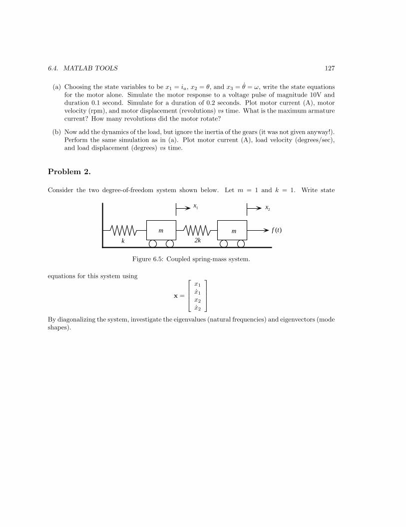
6.4. MATLAB TOOLS 127
(a) Choosing the state variables to be x1 = ia, x2 = θ, and x3 = θ = ω, write the state equationsfor the motor alone. Simulate the motor response to a voltage pulse of magnitude 10V andduration 0.1 second. Simulate for a duration of 0.2 seconds. Plot motor current (A), motorvelocity (rpm), and motor displacement (revolutions) vs time. What is the maximum armaturecurrent? How many revolutions did the motor rotate?
(b) Now add the dynamics of the load, but ignore the inertia of the gears (it was not given anyway!).Perform the same simulation as in (a). Plot motor current (A), load velocity (degrees/sec),and load displacement (degrees) vs time.
Problem 2.
Consider the two degree-of-freedom system shown below. Let m = 1 and k = 1. Write state
k 2k
m m f (t)
x1 x2
Figure 6.5: Coupled spring-mass system.
equations for this system using
x =
x1
x1
x2
x2
By diagonalizing the system, investigate the eigenvalues (natural frequencies) and eigenvectors (modeshapes).

128 CHAPTER 6. STATE-SPACE ANALYSIS OF CONTINUOUS SYSTEMS
Chapter 7
Digital Controller Design usingState Space Methods
7.1 Introduction
The state variable modeling approach presented in the previous chapter can also be applied in thediscrete domain. We will first examine state-space discrete models, then look at state feedbackcontrols laws, in which the control force u is a linear combination of the measured state variables.Using state feedback, the system poles can be placed arbitrarily. Since the entire state vector isusually not accessible, a state estimator must be developed. It will be shown that the poles of theoverall system are those of the control law plus those of the estimator. Introduction of the referenceinput will be the final chapter topic.
7.2 Canonical State-Space Forms from Transfer Function
It is easy to get a canonical discrete state-space model if you already have a discrete transfer function.That is not the typical path to follow when modeling, but it is worthwhile to discuss.
Consider the transfer function given by
G(z) =Y (z)
U(z)=b0 + b1z
−1 + b2z−2 + b3z
−3
1− a1z−1 − a2z−2 − a3z−3=b(z)
a(z)(7.1)
where the presence of b0 indicates a direct “feed-through” term. This was included because it isoften present in discrete-domain controllers.
Polynomials a(z) and b(z) can be separated using the block diagram of Figure 7.1(a) and theintroduction of intermediate variable vk with transform V (z). Thus
129

130 CHAPTER 7. DIGITAL CONTROLLER DESIGN USING STATE SPACE METHODS
U(z ) V(z) Y (z)1
a(z)b(z)
(a) Introduction of v.
a1
a2
+
a3
+ ++
z−1 z−1 z−1uk
vk vk −1 vk −2vk −3
(b) Addition of a terms.
a1
a2
+
b0
b1
b2
+
+ +
x3x2x1
b3
++
uk vk
a3
yk
z−1 z−1 z−1
(c) Addition of b terms.
Figure 7.1: Control Canonical Form.
V (z) =U(z)
a(z)or U(z) = a(z)V (z)
and
uk = vk − a1vk−1 − a2vk−2 − a3vk−3
or
vk = a1vk−1 + a2vk−2 + a3vk−3 + uk
and the block diagram in Figure 7.1(b) results. The delay elements are analogous to integrators forcontinuous systems.
To form the output yk use Y (z) = b(z)V (z), which leads to
yk = b0vk + b1vk−1 + b2vk−2 + b3vk−3.
which is shown in the block diagram in Figure 7.1(c)
Discrete State Equations. To avoid confusion with the continuous system and input matrices,we’ll use symbols Φ and Γ instead of A and B. The discrete state and output equations are:
x(k + 1) = Φx(k) + Γu(k) (7.2)
y(k) = Cx(k) +Du(k) (7.3)
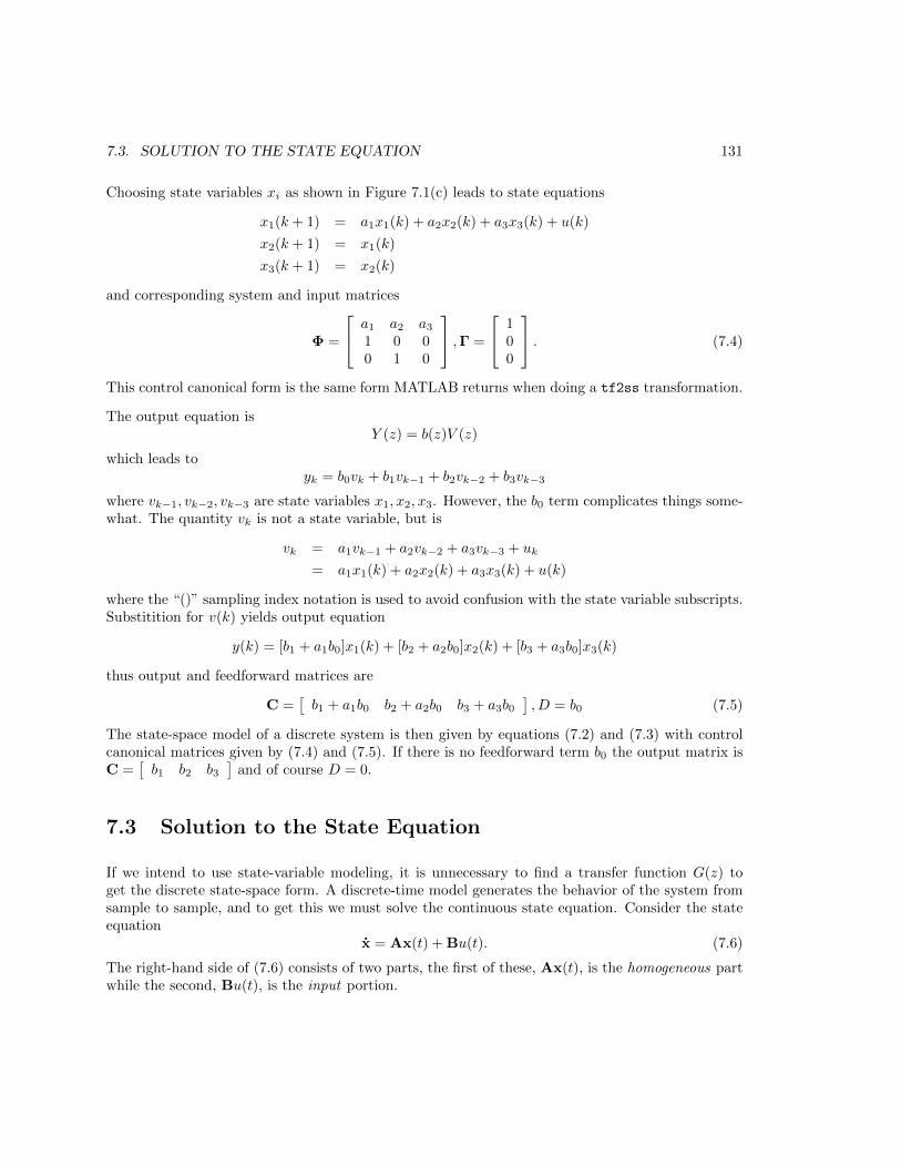
7.3. SOLUTION TO THE STATE EQUATION 131
Choosing state variables xi as shown in Figure 7.1(c) leads to state equations
x1(k + 1) = a1x1(k) + a2x2(k) + a3x3(k) + u(k)
x2(k + 1) = x1(k)
x3(k + 1) = x2(k)
and corresponding system and input matrices
Φ =
a1 a2 a3
1 0 00 1 0
,Γ =
100
. (7.4)
This control canonical form is the same form MATLAB returns when doing a tf2ss transformation.
The output equation isY (z) = b(z)V (z)
which leads toyk = b0vk + b1vk−1 + b2vk−2 + b3vk−3
where vk−1, vk−2, vk−3 are state variables x1, x2, x3. However, the b0 term complicates things some-what. The quantity vk is not a state variable, but is
vk = a1vk−1 + a2vk−2 + a3vk−3 + uk
= a1x1(k) + a2x2(k) + a3x3(k) + u(k)
where the “()” sampling index notation is used to avoid confusion with the state variable subscripts.Substitition for v(k) yields output equation
y(k) = [b1 + a1b0]x1(k) + [b2 + a2b0]x2(k) + [b3 + a3b0]x3(k)
thus output and feedforward matrices are
C =[b1 + a1b0 b2 + a2b0 b3 + a3b0
], D = b0 (7.5)
The state-space model of a discrete system is then given by equations (7.2) and (7.3) with controlcanonical matrices given by (7.4) and (7.5). If there is no feedforward term b0 the output matrix isC =
[b1 b2 b3
]and of course D = 0.
7.3 Solution to the State Equation
If we intend to use state-variable modeling, it is unnecessary to find a transfer function G(z) toget the discrete state-space form. A discrete-time model generates the behavior of the system fromsample to sample, and to get this we must solve the continuous state equation. Consider the stateequation
x = Ax(t) + Bu(t). (7.6)
The right-hand side of (7.6) consists of two parts, the first of these, Ax(t), is the homogeneous partwhile the second, Bu(t), is the input portion.
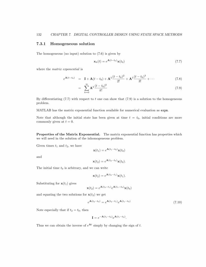
132 CHAPTER 7. DIGITAL CONTROLLER DESIGN USING STATE SPACE METHODS
7.3.1 Homogeneous solution
The homogeneous (no input) solution to (7.6) is given by
xh(t) = eA(t−t0)x(t0) (7.7)
where the matrix exponential is
eA(t−t0) = I + A(t− t0) + A2 (t− t0)2
2!+ A3 (t− t0)3
3!+ · · · (7.8)
=
∞∑k=0
Ak (t− t0)k
k!(7.9)
By differentiating (7.7) with respect to t one can show that (7.9) is a solution to the homogeneousproblem.
MATLAB has the matrix exponential function available for numerical evaluation as expm.
Note that although the initial state has been given at time t = t0, initial conditions are morecommonly given at t = 0.
Properties of the Matrix Exponential. The matrix exponential function has properties whichwe will need in the solution of the inhomogeneous problem.
Given times t1 and t2, we have
x(t1) = eA(t1−t0)x(t0)
and
x(t2) = eA(t2−t0)x(t0).
The initial time t0 is arbitrary, and we can write
x(t2) = eA(t2−t1)x(t1).
Substituting for x(t1) gives
x(t2) = eA(t2−t1)eA(t1−t0)x(t0)
and equating the two solutions for x(t2) we get
eA(t2−t0) = eA(t2−t1)eA(t1−t0) (7.10)
Note especially that if t2 = t0, then
I = e−A(t1−t0)eA(t1−t0).
Thus we can obtain the inverse of eAt simply by changing the sign of t.
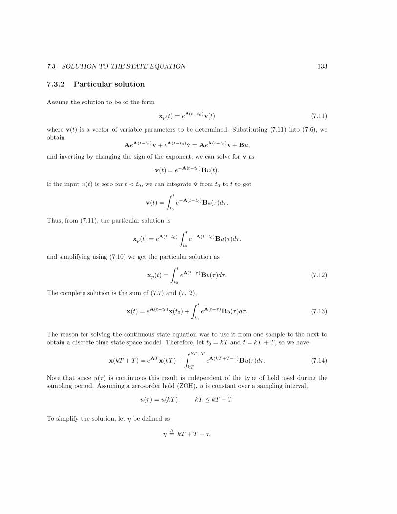
7.3. SOLUTION TO THE STATE EQUATION 133
7.3.2 Particular solution
Assume the solution to be of the form
xp(t) = eA(t−t0)v(t) (7.11)
where v(t) is a vector of variable parameters to be determined. Substituting (7.11) into (7.6), weobtain
AeA(t−t0)v + eA(t−t0)v = AeA(t−t0)v + Bu,
and inverting by changing the sign of the exponent, we can solve for v as
v(t) = e−A(t−t0)Bu(t).
If the input u(t) is zero for t < t0, we can integrate v from t0 to t to get
v(t) =
∫ t
t0
e−A(t−t0)Bu(τ)dτ.
Thus, from (7.11), the particular solution is
xp(t) = eA(t−t0)
∫ t
t0
e−A(t−t0)Bu(τ)dτ.
and simplifying using (7.10) we get the particular solution as
xp(t) =
∫ t
t0
eA(t−τ)Bu(τ)dτ. (7.12)
The complete solution is the sum of (7.7) and (7.12),
x(t) = eA(t−t0)x(t0) +
∫ t
t0
eA(t−τ)Bu(τ)dτ. (7.13)
The reason for solving the continuous state equation was to use it from one sample to the next toobtain a discrete-time state-space model. Therefore, let t0 = kT and t = kT + T , so we have
x(kT + T ) = eATx(kT ) +
∫ kT+T
kT
eA(kT+T−τ)Bu(τ)dτ. (7.14)
Note that since u(τ) is continuous this result is independent of the type of hold used during thesampling period. Assuming a zero-order hold (ZOH), u is constant over a sampling interval,
u(τ) = u(kT ), kT ≤ kT + T.
To simplify the solution, let η be defined as
η∆= kT + T − τ.

134 CHAPTER 7. DIGITAL CONTROLLER DESIGN USING STATE SPACE METHODS
Then we have
x(kT + T ) = eATx(kT ) +
∫ T
0
eAηdηBu(kT ). (7.15)
If we define
Φ∆= eAT , (7.16)
Γ∆=
∫ T
0
eAηdηB, (7.17)
we have from (7.15) the discrete state equation (and accompanying output equation),
x(k + 1) = Φx(k) + Γu(k) (7.18)
y(k) = Cx(k) (7.19)
which we got in Section 7.2.
7.3.3 Calculating system and output matrices
Both matrices Φ and Γ can be found using the matrix exponential series. Let the series for n × nmatrix Ψ be
Ψ∆= I +
AT
2!+
A2T 2
3!+ · · ·
then from the definition of the matrix exponential Φ is given by
Φ = I + ATΨ (7.20)
and the Γ integral in (7.17) can be evaluated term-by-term to give
Γ = ΨTB (7.21)
The (overloaded) MATLAB function c2d works on state-space models, too, so that is an easy wayto effect the discretization in the state variable domain. We will use the ‘zoh’ option.
SYSD = C2D(SYSC,Ts,METHOD) converts the continuous-time LTI
model SYSC to a discrete-time model SYSD with sample time Ts.
The string METHOD selects the discretization method among the
following:
’zoh’ Zero-order hold on the inputs
’foh’ Linear interpolation of inputs (triangle appx.)
’imp’ Impulse-invariant discretization
’tustin’ Bilinear (Tustin) approximation
’prewarp’ Tustin approximation with frequency prewarping.
The critical frequency Wc (in rad/sec) is specified
as fourth input by
SYSD = C2D(SYSC,Ts,’prewarp’,Wc)
’matched’ Matched pole-zero method (for SISO systems only).
The default is ’zoh’ when METHOD is omitted.

7.4. CONTROL LAW DESIGN 135
7.4 Control Law Design
One of the attractive features of state-space design methods is that the procedure consists of twoindependent steps. The first step assumes that we can measure all the states for control purposes,e.g. the state is accessible. In general this is not true, nevertheless we will formulate a control lawwith this assumption. The second step is to design a state “estimator” (sometimes referred to asan “observer”) which estimates the entire state vector based on a measurement of the (accessible)output given by
y = Cx +Du (where D is usually zero for physical systems)
The final controller will consist of the combination of the control law and the estimator, with thecontrol computed using the estimated states.
The most general linear state control law is simply a linear combination of all state variables, thatis:
u = −Kx = −[K1 K2 · · · Kn
]x1
x2
...xn
(7.22)
This control law does not provide for a reference input to the system, hence r = 0, and such a systemis a regulator.
Recall that the plant discrete state equation is
x(k + 1) = Φx(k) + Γu(k) (7.23)
Substituting (7.22) into (7.23) we get
x(k + 1) = Φx(k)− ΓKx(k). (7.24)
Taking the z-transform of (7.24) produces
(zI−Φ + ΓK)X(z) = 0
For a non-trivial solution for X(z) to exist for the above equation, the determinant must be zero,that is,
|zI−Φ + ΓK| = 0 (7.25)
Equation (7.25) is the characteristic equation of the plant+control law.
7.4.1 Pole Placement
We will use the method of pole placement, since our control law has as many unknown parame-ters (the Ki), we are able to place the closed-loop poles (eigenvalues) arbitrarily. Note that this

136 CHAPTER 7. DIGITAL CONTROLLER DESIGN USING STATE SPACE METHODS
places a burden on the designer to select reasonable closed-loop pole locations. Unlike transform-based design—which often involves iteration—the full state feedback, pole placement approach hasguaranteed success.
Let the desired pole locations bezi = p1, p2, . . ., pn
then the characteristic equation is
αc(z) = (z − p1)(z − p2)· · ·(z − pn) = 0 (7.26)
Since (7.25) and (7.26) are both characteristic equations of the controlled system, they must beidentical. Since equation (7.26) is known (we pick the pole locations) and equation (7.25) is symbolic,we can equate coefficients of like powers of z in both equations, and n simultaneous equations forthe Ki will result.
Example
Consider the plant given by
G(s) =Y (s)
U(s)=
1
s2
which represents a pure inertia. With two poles at the origin, this plant is unstable. Suppose wewish to design a control law for this plant so the poles have
ζ = 0.707
ωn = 10 rad/sec
which corresponds to poles at s = −7.07± j7.07.
Pick a sample period of T = 0.1 second, this is about six times the desired natural frequency. Lettingthe state vector be
x =
[x1
x2
]=
[yy
]the state equations are
x1 = x2
x2 = u
and the output is simply y = u, hence the continuous state-space matrices are
A =
[0 10 0
],B =
[01
],C =
[1 0
], D = 0.
Discretizing the system at T = 0.1 second, we obtain
Φ =
[1 0.10 1
],Γ =
[0.0050.1
]
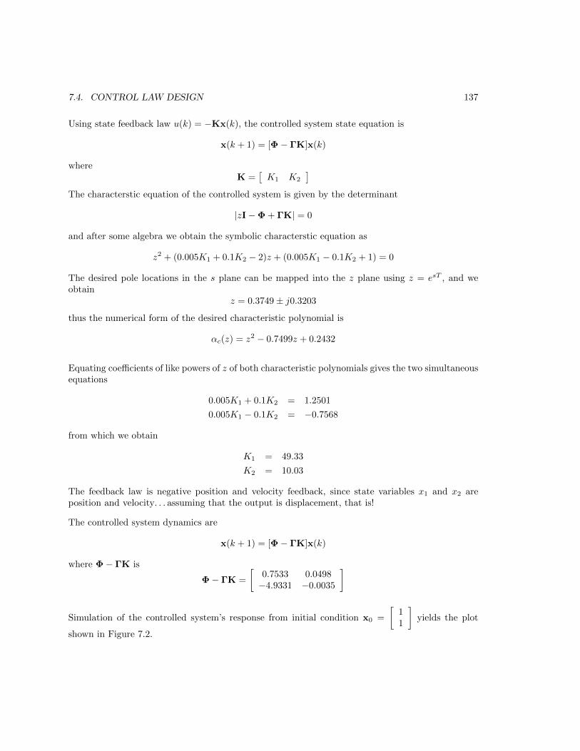
7.4. CONTROL LAW DESIGN 137
Using state feedback law u(k) = −Kx(k), the controlled system state equation is
x(k + 1) = [Φ− ΓK]x(k)
whereK =
[K1 K2
]The characterstic equation of the controlled system is given by the determinant
|zI−Φ + ΓK| = 0
and after some algebra we obtain the symbolic characterstic equation as
z2 + (0.005K1 + 0.1K2 − 2)z + (0.005K1 − 0.1K2 + 1) = 0
The desired pole locations in the s plane can be mapped into the z plane using z = esT , and weobtain
z = 0.3749± j0.3203
thus the numerical form of the desired characteristic polynomial is
αc(z) = z2 − 0.7499z + 0.2432
Equating coefficients of like powers of z of both characteristic polynomials gives the two simultaneousequations
0.005K1 + 0.1K2 = 1.2501
0.005K1 − 0.1K2 = −0.7568
from which we obtain
K1 = 49.33
K2 = 10.03
The feedback law is negative position and velocity feedback, since state variables x1 and x2 areposition and velocity. . . assuming that the output is displacement, that is!
The controlled system dynamics are
x(k + 1) = [Φ− ΓK]x(k)
where Φ− ΓK is
Φ− ΓK =
[0.7533 0.0498−4.9331 −0.0035
]
Simulation of the controlled system’s response from initial condition x0 =
[11
]yields the plot
shown in Figure 7.2.

138 CHAPTER 7. DIGITAL CONTROLLER DESIGN USING STATE SPACE METHODS
0 0.2 0.4 0.6 0.8 1-0.2
0
0.2
0.4
0.6
0.8
1
Time (seconds)Figure 7.2: Response of controlled inertia plant from initial condi-tion x(0) = [1 1]T .
7.4.2 Selecting System Pole Locations
While the selection of the desired system pole locations is highly application-specific, there are someguidelines. Generally, it is unwise to expect the closed-loop system to respond dramatically fasterthan the slowest component in the loop. Feedback control can improve system dynamics (overshoot,stability, etc.), but requesting closed-loop response that is much faster than the slowest componentresponse (often the plant) may saturate one or more components. Simulation is always beneficial toexplore the limits of system performance.
7.4.3 Controllability and the Control Canonical Form
The algebra for finding the state feedback gain matrix K is especially simple if the system matriceshappen to be in control canonical form. Recall for a third order system (with no feed-through termb0), this form was:
Φc =
a1 a2 a3
1 0 00 1 0
,Γc =
100
,Cc =[b1 b2 b3
]. (7.27)
7.4. CONTROL LAW DESIGN 139
The characteristic polynomial of equation (7.27) is z3 − a1z2 − a2z − a3. The key idea here is that
the elements of the first row of Φc are exactly the coefficients of the characteristic polynomial of thesystem. If we now form the closed-loop system matrix Φc − ΓcK, we find
Φc − ΓcK =
a1 −K1 a2 −K2 a3 −K3
1 0 00 1 0
. (7.28)
By inspection, the characteristic equation of (7.28) is
z3 − (a1 −K1)z2 − (a2 −K2)z − (a3 −K3) = 0
Thus, if the desired pole locations result in the characteristic equation
z3 − α1z2 − α2z − α3 = 0,
the necessary values for the control gains are
K1 = a1 − α1, K2 = a2 − α2, K3 = a3 − α3. (7.29)
This leads to a design method: Given an arbitrary (Φ,Γ), and a desired characteristic equationα(z) = 0, convert (by redefinition of the state vector) to control canonical form (Φc,Γc), and solvefor the gain by (7.29). Since this gain is for states in the control canonical form, we must expressthe result back in terms of the original state vector.
Is it always possible to find the control canonical form? Yes, almost always, but there are certainpathological systems called “uncontrollable” for which no control will give arbitrary root locations.These systems have certain modes or subsystems which are unaffected by the control.
If all roots are distinct, the system can be diagonalized using the matrix of eigenvectors as discussedin the previous chapter. The system is then
x(k + 1) =
λ1
λ2
. . .
λn
x(k) +
Γ1
Γ2
...Γn
u(k) (7.30)
and explicitly exhibits the criterion for controllability: when in this form, no element of Γ can bezero. If any Γ element were zero, no control would influence that mode directly and the associatedstate would remain uncontrolled.
7.4.4 Ackermann’s Rule and a Test for Controllability
There is a mathematical test for controllability, although the details will not be presented here. Thetest is:
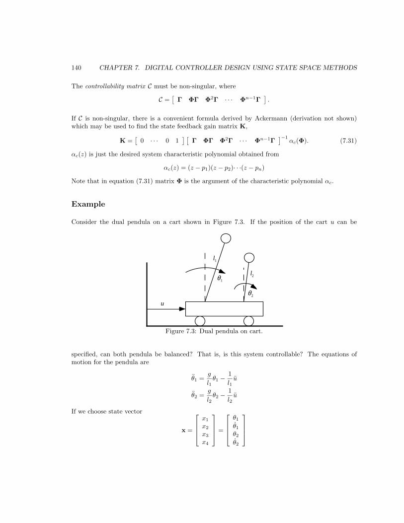
140 CHAPTER 7. DIGITAL CONTROLLER DESIGN USING STATE SPACE METHODS
The controllability matrix C must be non-singular, where
C =[
Γ ΦΓ Φ2Γ · · · Φn−1Γ].
If C is non-singular, there is a convenient formula derived by Ackermann (derivation not shown)which may be used to find the state feedback gain matrix K,
K =[
0 · · · 0 1] [
Γ ΦΓ Φ2Γ · · · Φn−1Γ]−1
αc(Φ). (7.31)
αc(z) is just the desired system characteristic polynomial obtained from
αc(z) = (z − p1)(z − p2)· · ·(z − pn)
Note that in equation (7.31) matrix Φ is the argument of the characteristic polynomial αc.
Example
Consider the dual pendula on a cart shown in Figure 7.3. If the position of the cart u can be
u
l1
l2θ1
θ2
Figure 7.3: Dual pendula on cart.
specified, can both pendula be balanced? That is, is this system controllable? The equations ofmotion for the pendula are
θ1 =g
l1θ1 −
1
l1u
θ2 =g
l2θ2 −
1
l2u
If we choose state vector
x =
x1
x2
x3
x4
=
θ1
θ1
θ2
θ2
7.4. CONTROL LAW DESIGN 141
and let the input be u for simplicity, we have system matrix A and input matrix B as
A =
0 1 0 0g/l1 0 0 0
0 0 0 10 0 g/l2 0
,B =
0
−1/l10
−1/l2
The controllability matrix C for continuous systems is exactly the same as for discrete,
C =[
B AB A2B · · ·]
and C for the dual pendula system is
C =
0 −1/l1 0 −g/l21
−1/l1 0 −g/l21 00 −1/l2 0 −g/l22
−1/l2 0 −g/l22 0
It can be shown that if l1 = l2 the rank of C is 3, but if l1 6= l2 the rank of C is 4. Hence if the twopendula are the same length, this system is uncontrollable.
7.4.5 MATLAB Tools
If numerical values are available, here are two MATLAB functions that can assist control law design:place and ctrb:
place. Ackermann’s rule is invoked by function place:
PLACE Pole placement technique
K = PLACE(A,B,P) computes a state-feedback matrix K such that
the eigenvalues of A-B*K are those specified in vector P.
No eigenvalue should have a multiplicity greater than the
number of inputs.
[K,PREC,MESSAGE] = PLACE(A,B,P) returns PREC, an estimate of how
closely the eigenvalues of A-B*K match the specified locations P
(PREC measures the number of accurate decimal digits in the actual
closed-loop poles). If some nonzero closed-loop pole is more than
10% off from the desired location, MESSAGE contains a warning
message.

142 CHAPTER 7. DIGITAL CONTROLLER DESIGN USING STATE SPACE METHODS
ctrb. Form the controllability matrix.
CTRB Compute the controllability matrix.
CO = CTRB(A,B) returns the controllability matrix [B AB A^2B ...].
CO = CTRB(SYS) returns the controllability matrix of the
state-space model SYS with realization (A,B,C,D). This is
equivalent to CTRB(sys.a,sys.b).
Controllability may be checked by finding the rank of the controllability matrix C. If C has less thanfull rank, the system is uncontrollable.
7.4.6 Poles and Zeros
It is worthwhile to consider the poles and zeros of a system using the state-space model. Considerthe plant state and output equations
x(k + 1 = Φx(k) + Γu(k)
y(k) = Cx(k),
which may be z-transformed, giving
[zI−Φ]X(x) = ΓU(z)
Y (z) = CX(z)
From these two equations we can solve for the transfer function
Y (z)
U(z)= C[zI−Φ]−1Γ.
Pole locations are values of z such that the plant can have an output with no input, this is just thenatural response. This can only happen if
|zI−Φ| = 0,
which is the characteristic equation of the plant. Roots of this equation are the poles. We have usedthis approach in solving for the control gains.
Zeros are values of z such that the output y is zero with a non-zero input and state vector x. Thiscan be expressed in matrix form,[
zI−Φ −ΓC 0
] [X(z)U(z)
]=
[0
Y (z)
]=
[00
]For a non-zero state X(z) and input U(z), the following determinant must be zero:∣∣∣∣ zI−Φ −Γ
C 0
∣∣∣∣ = 0 (7.32)
Then equation (7.32) will yield the zeros. Note that with pole placement we have no control of theeventual locations of the system zeros.

7.4. CONTROL LAW DESIGN 143
Homework Problem Set 1
Problem 1.
For the example of Section 7.4, where G(s) = 1/s2, compute Φ and Γ using the series expansionsof equations (7.20) and (7.21). Verify with the example.
Problem 2.
Design a state feedback control law for the DC motor + inertia of Chapter 6, Problem 1. Pickdesired system pole locations consistent with the physical limitations of the system. Simulate thesystem’s response to an initial condition.
7.4.7 More on Controllability
We stated in Section 7.4.4 that a system was controllable if the matrix
C ∆=[
Γ ΦΓ · · · Φn−1Γ]
is nonsingular. Let us examine controllability a little more deeply. Consider the statement
The system (Φ,Γ) is controllable if for every xi and xf there is a finite N and a set ofcontrols u(0), u(1) . . . u(N) such that if the system has state xi at k = 0, it is forced tostate xf at k = N .
The system state equation isx(k + 1) = Φx(k) + Γu(k).
Solving this equation for a few steps, we find
x(1) = Φxi + Γu(0)
x(2) = Φx(1) + Γu(1)
= Φ2xi + ΦΓu(0) + Γu(1)
...
x(N) = ΦNxi +[
Γ ΦΓ · · · ΦN−1Γ] u(N − 1)
...u(0)
If x(N) is to equal xf , then we must be able to solve the equations
[Γ ΦΓ · · · ΦN−1Γ
]u(N − 1)u(N − 2)
...u(0)
= xf −ΦNxi
144 CHAPTER 7. DIGITAL CONTROLLER DESIGN USING STATE SPACE METHODS
for the control sequence u(k).
The “coefficient” matrix is just our controllability matrix C, and it has n rows and N columns. IfN < n we cannot find a solution for general xf . And if N > n we add additional columns, andsolution existence is not readily apparent. But note that Γ can be factored out of C to the right, weare left with increasing powers of Φ, as[
I Φ Φ2 · · ·].
But the Cayley-Hamilton theorem says (in a nutshell) that a matrix Φ satisfies its own characteristicpolynomial, this can be rearranged to say that Φn is a linear combination of lower powers of Φ,thus the additional columns if N > n do not increase the rank. Therefore we have a solution for thecontrol sequence if and only if the rank of C is n.
7.5 State Estimator Design
The state feedback control law as used in the previous section presumed that the state was accessible.In fact, this is not likely to be true, and the missing portion of the state (or the entire state) needsto be constructed from the measured output. If the state vector is x, the state estimate will be x,and the control law will use the estimate, u = −Kx.
NOTE: In this section we make a distinction between output y and measurable output ym. Thetwo are usually the same, but there could be a situation in which they are different. Measurableoutput ym has with it a corresponding Cm output matrix.
7.5.1 Prediction Estimator
Since we have a model of the plant dynamics, one way to estimate the state is just use this model,
x(k + 1) = Φx(k) + Γu(k) (7.33)
where x denotes the state estimate. The input u(k) is known, as are Φ and Γ, so if the state estimatecan be accurately initialized, x(0) = x(0), this should work. Let’s see. . .
Figure 7.4 shows this “open-loop” estimator. Define the estimator error by
x∆= x− x (7.34)
and it can be shown by subtracting (7.33) from the plant state equation (7.2) that
x(k + 1) = Φx(k). (7.35)
This says that the dynamics of the estimator error are identical to those of the uncontrolled plant!If there is any initial error in the state estimate, that error will propagate with dynamics identicalto those of the uncontrolled plant. Needless to say, this is undesirable.

7.5. STATE ESTIMATOR DESIGN 145
Plant
Model
Φ, Γ
Φ, Γ
x(0)
x(0)
u(k ) x(k)
x(k)
y(k)
y(k)
C
C
Figure 7.4: Open-loop estimator.
Plant
Model
Φ, Γ
Φ, Γ
u(k ) x(k)
x(k)
y(k)
y(k)
C
C+
-
L
Figure 7.5: Closed-loop estimator.
The solution is to use the difference between the measured output y and the estimated output y tocorrect the estimator. This is shown in Figure 7.5. The estimated output is ym(k) = Cmx(k), andthe difference equation for the closed-loop estimator is
x(k + 1) = Φx(k) + Γu(k) + L[ym(k)−Cmx(k)] (7.36)
This is called a prediction estimator because the state estimate x(k+ 1) is one sample ahead of themeasurement ym(k). Matrix L contains the estimator feedback gains which will (hopefully) improveestimator performance.
The difference equation for estimator error can again be found by subtracting equation (7.36) from(7.2), and we get
x(k + 1) = [Φ− LCm]x(k) (7.37)
The dynamics of this system are given by [Φ− LCm], and if we select L so this estimator has afast stable response, any initial state estimate errors will be driven to zero. Thus the state estimatex(k) will converge to the actual state x(k).
146 CHAPTER 7. DIGITAL CONTROLLER DESIGN USING STATE SPACE METHODS
We can find L the same way we found K, by taking the z-transform of equation (7.37) to get
[zI−Φ + LCm]X(z) = 0
then the symbolic estimator error characteristic equation is given by
|zI−Φ + LCm| = 0 (7.38)
The desired poles for the estimator error dynamics will yield numerical characteristic polynomialαe(z), then coefficients between the two polynomials can be equated to yield n simultaneous equa-tions in the estimator gains Li.
Estimator pole locations. Typically, estimator pole locations are selected so that the estimatorresponds two to six times faster than the controlled plant. If there is noise on the measurement,slower estimation is required.
7.5.2 Observability and Ackermann’s Formula
Given a desired set of estimator poles, does gain matrix L exist? As with controllability, it usuallyexists, but it may not. The key idea is whether by only a measurement of the output y we candeduce the behavior of the entire state vector x. If all internal modes are “connected” to the output,the system is observable.
Ackermann’s formula can be used for estimator gain matrix computation, it is
L = αe(Φ)
Cm
CmΦ
CmΦ2
...
CmΦn−1
−1 00...01
(7.39)
In equation (7.39) we find the observability matrix O to be
O =[
Cm CmΦ CmΦ2 · · · CmΦn−1]. (7.40)
This matrix must be full rank (nonsingular) for the system to be controllable.
7.5.3 MATLAB Tools
If we take the transpose of the estimator error equation system matrix Φ− LCm, we get ΦT −Cm
TLT , which is the same form as system matrix Φ− ΓK, so if we substitute ΦT for Φ, CmT
for Γ, and LT for K, we can use the same approach for estimator gain computation as for controlgains. Specifically, MATLAB function place may be used. Design of a prediction estimator usingMATLAB will be shown in the next section.
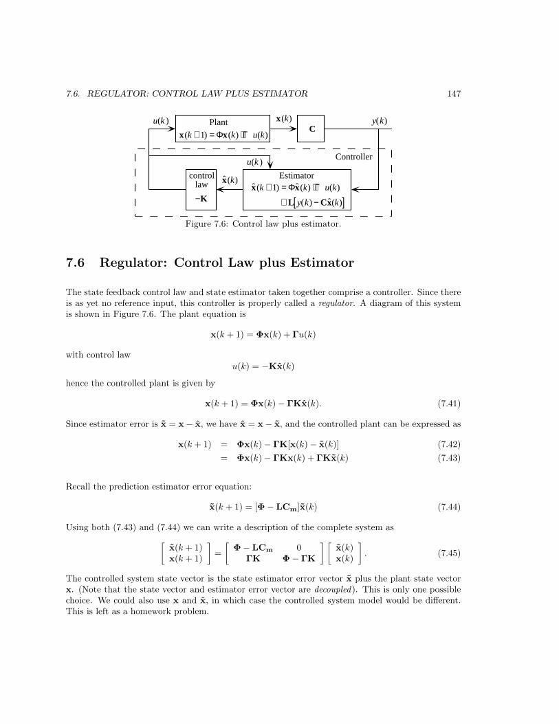
7.6. REGULATOR: CONTROL LAW PLUS ESTIMATOR 147
x(k + 1) = Φx(k) + Γu(k)
+ L y(k) − Cx(k)[ ]
Estimator
x(k + 1) = Φx(k) + Γu(k)
PlantC
−K
controllaw
u(k ) x(k) y(k)
x(k)
u(k )Controller
Figure 7.6: Control law plus estimator.
7.6 Regulator: Control Law plus Estimator
The state feedback control law and state estimator taken together comprise a controller. Since thereis as yet no reference input, this controller is properly called a regulator. A diagram of this systemis shown in Figure 7.6. The plant equation is
x(k + 1) = Φx(k) + Γu(k)
with control law
u(k) = −Kx(k)
hence the controlled plant is given by
x(k + 1) = Φx(k)− ΓKx(k). (7.41)
Since estimator error is x = x− x, we have x = x− x, and the controlled plant can be expressed as
x(k + 1) = Φx(k)− ΓK[x(k)− x(k)] (7.42)
= Φx(k)− ΓKx(k) + ΓKx(k) (7.43)
Recall the prediction estimator error equation:
x(k + 1) = [Φ− LCm]x(k) (7.44)
Using both (7.43) and (7.44) we can write a description of the complete system as[x(k + 1)x(k + 1)
]=
[Φ− LCm 0
ΓK Φ− ΓK
] [x(k)x(k)
]. (7.45)
The controlled system state vector is the state estimator error vector x plus the plant state vectorx. (Note that the state vector and estimator error vector are decoupled). This is only one possiblechoice. We could also use x and x, in which case the controlled system model would be different.This is left as a homework problem.
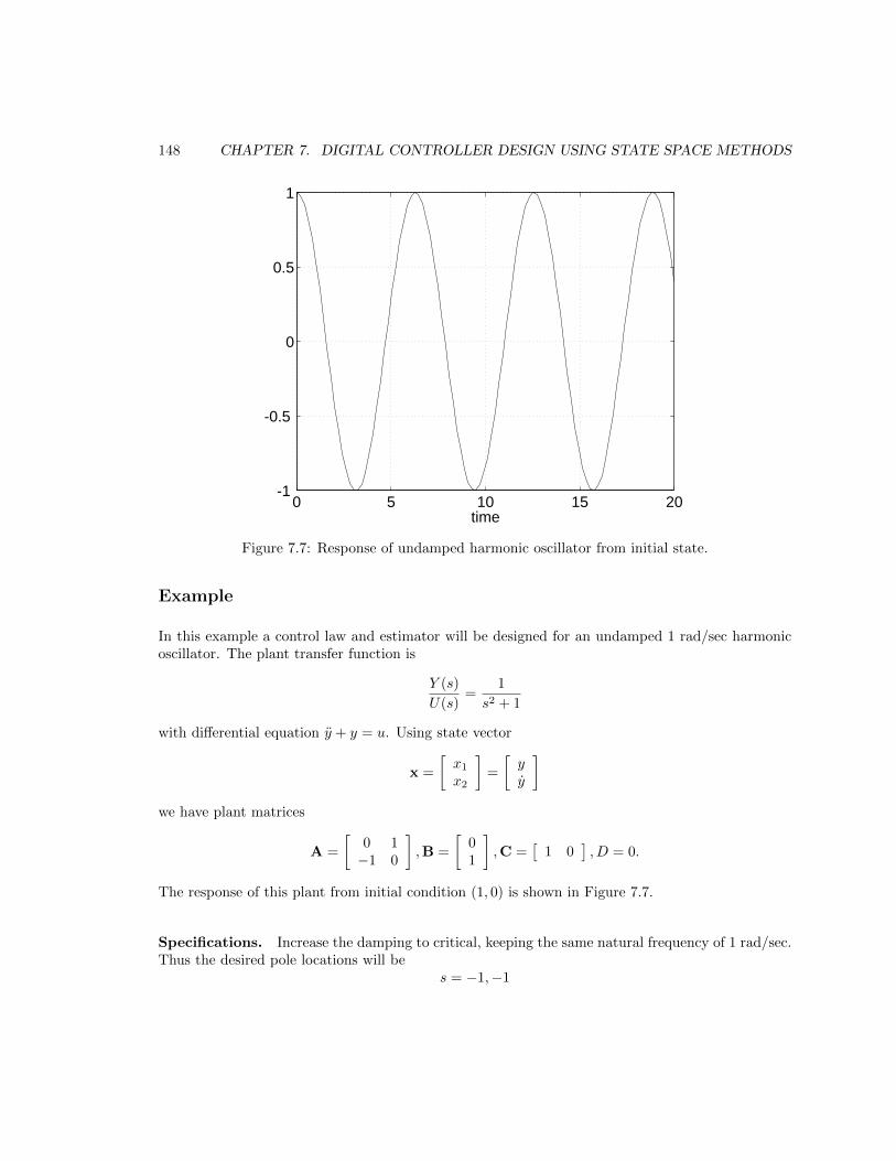
148 CHAPTER 7. DIGITAL CONTROLLER DESIGN USING STATE SPACE METHODS
0 5 10 15 20-1
-0.5
0
0.5
1
time
Figure 7.7: Response of undamped harmonic oscillator from initial state.
Example
In this example a control law and estimator will be designed for an undamped 1 rad/sec harmonicoscillator. The plant transfer function is
Y (s)
U(s)=
1
s2 + 1
with differential equation y + y = u. Using state vector
x =
[x1
x2
]=
[yy
]we have plant matrices
A =
[0 1−1 0
],B =
[01
],C =
[1 0
], D = 0.
The response of this plant from initial condition (1, 0) is shown in Figure 7.7.
Specifications. Increase the damping to critical, keeping the same natural frequency of 1 rad/sec.Thus the desired pole locations will be
s = −1,−1

7.6. REGULATOR: CONTROL LAW PLUS ESTIMATOR 149
Sampling period. The controlled system will have natural frequency of 1 rad/sec, or about 1/6Hz. Pick sampling frequency to be approximately six times this frequency, or 1 Hz. Hence T = 1.
Plant Discretization. Using this T , the continuous plant can be defined, then discretized usingMATLAB:
>> A = [0 1;-1 0];
>> B = [0;1];
>> C = [1 0];
>> D = 0;
>>
>> plant_c = ss(A,B,C,D);
>> T = 1;
>> plant_d = c2d(plant_c,T)
a =
x1 x2
x1 0.5403 0.8415
x2 -0.8415 0.5403
b =
u1
x1 0.4597
x2 0.8415
c =
x1 x2
y1 1 0
d =
u1
y1 0
Sampling time: 1
Discrete-time model.
Note that the state-space matrices can be extracted from LTI model plant d by:
>> Phi = plant_d.A
Phi =
0.5403 0.8415
-0.8415 0.5403

150 CHAPTER 7. DIGITAL CONTROLLER DESIGN USING STATE SPACE METHODS
0 5 10 15 200
0.2
0.4
0.6
0.8
1
time
Figure 7.8: Response of controlled plant from initial state.
Control Law. The desired z-plane pole locations are found using the mapping z = esT ,
>>control_s_poles = [-1 -1]’;
>>control_z_poles = exp(control_s_poles*T)
control_z_poles = 0.3679
0.3679
It is a numerical anomaly of MATLAB function place that poles of multiplicity greater than thenumber of inputs are not allowed. One pole can therefore be offset slightly, and the gain vector K is
>>control_z_poles(1) = control_z_poles(1)+0.0001;
>>K = place(Phi,Gamma,control_z_poles)
place: ndigits= 19
K = -0.5655 0.7186
The control law u = −Kx is seen to be positive position feedback and negative velocity feedback.As a check, simulate the controlled system response from initial condition (1, 0). This is shown inFigure 7.8.
Prediction Estimator. Select the natural frequency of the prediction estimator to be five timesthe controlled plant, again with critical damping, thus the estimator pole locations are s = −5,−5,and
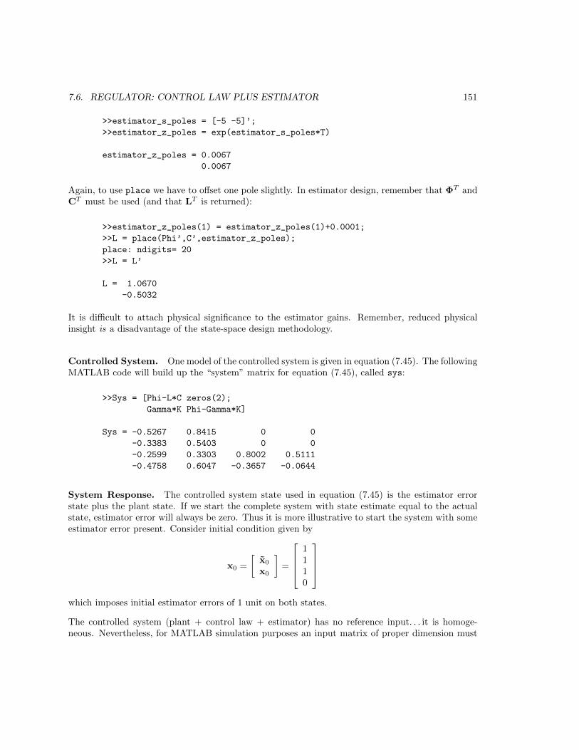
7.6. REGULATOR: CONTROL LAW PLUS ESTIMATOR 151
>>estimator_s_poles = [-5 -5]’;
>>estimator_z_poles = exp(estimator_s_poles*T)
estimator_z_poles = 0.0067
0.0067
Again, to use place we have to offset one pole slightly. In estimator design, remember that ΦT andCT must be used (and that LT is returned):
>>estimator_z_poles(1) = estimator_z_poles(1)+0.0001;
>>L = place(Phi’,C’,estimator_z_poles);
place: ndigits= 20
>>L = L’
L = 1.0670
-0.5032
It is difficult to attach physical significance to the estimator gains. Remember, reduced physicalinsight is a disadvantage of the state-space design methodology.
Controlled System. One model of the controlled system is given in equation (7.45). The followingMATLAB code will build up the “system” matrix for equation (7.45), called sys:
>>Sys = [Phi-L*C zeros(2);
Gamma*K Phi-Gamma*K]
Sys = -0.5267 0.8415 0 0
-0.3383 0.5403 0 0
-0.2599 0.3303 0.8002 0.5111
-0.4758 0.6047 -0.3657 -0.0644
System Response. The controlled system state used in equation (7.45) is the estimator errorstate plus the plant state. If we start the complete system with state estimate equal to the actualstate, estimator error will always be zero. Thus it is more illustrative to start the system with someestimator error present. Consider initial condition given by
x0 =
[x0
x0
]=
1110
which imposes initial estimator errors of 1 unit on both states.
The controlled system (plant + control law + estimator) has no reference input. . . it is homoge-neous. Nevertheless, for MATLAB simulation purposes an input matrix of proper dimension must
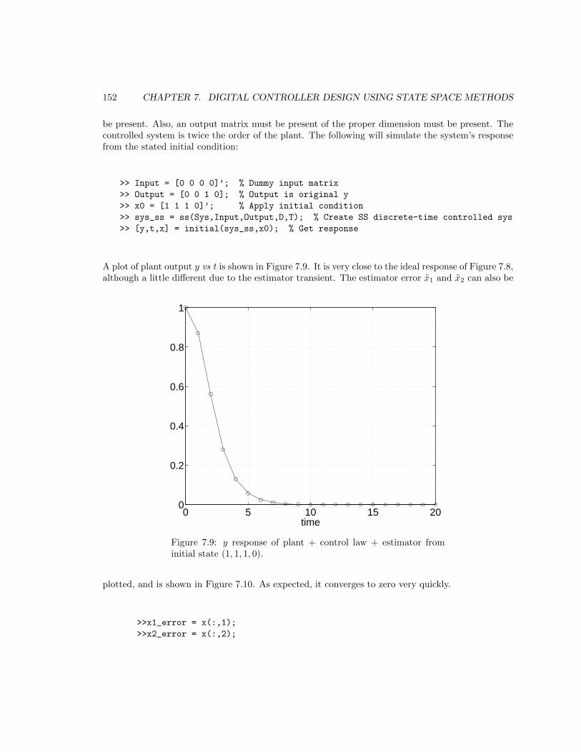
152 CHAPTER 7. DIGITAL CONTROLLER DESIGN USING STATE SPACE METHODS
be present. Also, an output matrix must be present of the proper dimension must be present. Thecontrolled system is twice the order of the plant. The following will simulate the system’s responsefrom the stated initial condition:
>> Input = [0 0 0 0]’; % Dummy input matrix
>> Output = [0 0 1 0]; % Output is original y
>> x0 = [1 1 1 0]’; % Apply initial condition
>> sys_ss = ss(Sys,Input,Output,D,T); % Create SS discrete-time controlled sys
>> [y,t,x] = initial(sys_ss,x0); % Get response
A plot of plant output y vs t is shown in Figure 7.9. It is very close to the ideal response of Figure 7.8,although a little different due to the estimator transient. The estimator error x1 and x2 can also be
0 5 10 15 200
0.2
0.4
0.6
0.8
1
time
Figure 7.9: y response of plant + control law + estimator frominitial state (1, 1, 1, 0).
plotted, and is shown in Figure 7.10. As expected, it converges to zero very quickly.
>>x1_error = x(:,1);
>>x2_error = x(:,2);

7.6. REGULATOR: CONTROL LAW PLUS ESTIMATOR 153
0 5 10 15 200
0.2
0.4
0.6
0.8
1
time
x1 estimator errorx2 estimator error
Figure 7.10: Estimator error response.
Homework Problem Set 2
Problem 1.
Derive the symbolic matrix equations like (7.45) but using
xsystem =
[xx
]as the controlled system state vector.
Problem 2.
Design a prediction state estimator for the DC motor + inertia of Problem 2 of the previous home-work set. Assume the measurement is y = θl. Pick desired estimator pole locations consistent withthe control law you determined (or the instructor’s). Perform appropriate simulations to demon-strate the successful behavior of your system.
154 CHAPTER 7. DIGITAL CONTROLLER DESIGN USING STATE SPACE METHODS
7.6.1 Controller Transfer Function
The controller contained within the dashed line of Figure 7.6 accepts a measurement y and generatesa control u. It is interesting to find the transfer function of the controller and verify it using transformmethods. Note that the controller transfer function need not be determined during a state-spacedesign effort.
We will consider a controller based on the prediction estimator. The prediction estimator updateequation (7.36) is
x(k + 1) = Φx(k) + Γu(k) + L[y(k)−Cx(k)] (7.46)
and the accompanying control law is
u(k) = −Kx(k) (7.47)
These two equations define the controller. To find the transfer function, substitute (7.47) in (7.46)and express
x(k + 1) = [Φ− ΓK− LC]x(k) + Ly(k). (7.48)
Equation (7.48) is the state equation for the controller, while equation (7.47) is the output equationfor the controller. Apply the z-transform to (7.48) to obtain
zX = [Φ− ΓK− LC]X + LY,
and solve for X as
X = [zI−Φ + ΓK + LC]−1LY.
Substitution of X into U = −KX yields the controller transfer function
U(z)
Y (z)= D(z) = −K[zI−Φ + ΓK + LC]
−1L (7.49)
MATLAB Tools. With controller state equation (7.48) and output equation (7.47) the “A,B,C,D”matrices can be identified and used in the ss2tf function to find the [num,den] transfer functionform. This will be shown in the following example.
Example
Consider the undamped oscillator of the previous sections. We discretized this system to obtain
Φ =
[0.5403 0.8415−0.8415 0.5403
],Γ =
[0.45970.8415
]and found control law and prediction estimator gains
K =[−0.5655 0.7186
],L =
[1.0670−0.5032
]

7.6. REGULATOR: CONTROL LAW PLUS ESTIMATOR 155
From (7.48) and (7.47) the equivalent state-space matrices for the controller are
Ac → Φ− ΓK− LC
Bc → L
Cc → −K
Dc → 0
and the MATLAB script below yields the controller transfer function.
>>Ac = Phi-Gamma*K-L*C;
>>Bc = L;
>>Cc = K;
>>Dc = 0;
>>[numc,denc] = ss2tf(Ac,Bc,Cc,Dc)
numc = 0 -0.9650 0.1156
denc = 1.0000 0.3311 -0.0531
>>[zeros_c,poles_c,K_c] = tf2zp(numc,denc)
zeros = 0.1198
poles = -0.4494
0.1183
K = 0.9650
Thus the controller transfer function is
D(z) =−0.965(z − 0.1198)
(z − 0.1183)(z + 0.4494)
A transfer function for the plant can be found by
>>[nump,denp] = ss2tf(Phi,Gamma,C,D)
nump = 0 0.4597 0.4597
denp = 1.0000 -1.0806 1.0000
>>[zeros_p,poles_p,K_p] = tf2zp(nump,denp)
zeros_p = -1
poles_p = 0.5403 + 0.8415i
0.5403 - 0.8415i
K_p = 0.4597

156 CHAPTER 7. DIGITAL CONTROLLER DESIGN USING STATE SPACE METHODS
−1 −0.5 0 0.5 1 1.5
−1
−0.5
0
0.5
1
Root Locus
Real Axis
Imag
inar
y A
xis
Figure 7.11: Root locus of oscillator plant and controller.
The plant transfer function is
G(z) =0.4597(z + 1)
z − 0.5403± j0.8415
Root Locus. Let the controller gain of 0.965 be replaced by a variable parameter 0.965K. Nowperform a root locus analysis of the plant with K as the parameter. This is shown in Figure 7.11along with the closed-loop poles when K = 1. The poles should be exactly at z = 0.3679(2) andz = 0.0067, the desired poles of the control law and estimator error dynamics! They’re prettyclose...science is wonderful!
7.7 Current and Reduced-Order Estimators
The prediction estimator as presented in Section 7.5.1 is only one possibility for state estimation.Two other approaches will be shown in this Section.
7.7. CURRENT AND REDUCED-ORDER ESTIMATORS 157
7.7.1 Current Estimator
Inspection of equation (7.36) shows that the state estimate at sample k + 1, x(k + 1), dependson measured system output y(k). Thus there is an inherent one sample delay between the newestimated state and the measurement used to correct it. Common sense tells us that it may improveestimation if we use the current value of measurement y(k + 1) to correct state estimate x(k + 1).
One would only use a current estimator if the control computer were fast enough to perform theestimator calculations very quickly, since this computation time is not modeled, and will thereforehave an effect on the system performance. If computational latency is significant, a predictionestimator may be a better choice.
To analyze the current estimator we will separate the estimate prediction from the estimate correc-tion. The prediction equation is simply the plant model,
x(k + 1) = Φx(k) + Γu(k) (7.50)
where x is the predicted state before correction.
The correction equation is
x(k + 1) = x(k + 1) + L[y(k + 1)−Cx(k + 1)] (7.51)
where x(k + 1) is the new state estimate.
Substitution of (7.50) into (7.51) results in the current estimator equation,
x(k + 1) = [Φ− LCΦ]x(k) + [Γ− LCΓ]u(k) + Ly(k + 1) (7.52)
Note that the coefficient matrices in (7.52) are constant, hence the current estimator of (7.52) is notmore computationally complex than the prediction estimator equation of (7.36).
The estimator error x∆= x− x as before, and subtracting equation (7.52) from plant equation (7.2)
yields the current estimator error equation,
x(k + 1) = [Φ− LCΦ]x(k) (7.53)
The poles of the current estimator error equation are given by
|zI−Φ + LCΦ| = 0,
and the symbolic characteristic obtained from this determinant may be equated with the desiredαe(z) = (z − p1)(z − p2) . . . to solve for current estimator gain matrix L.
Ackermann’s rule. Equation (7.53) for the current estimator is of the same form as (7.37) for theprediction estimator, except C is replaced by CΦ. Thus Ackermann’s rule for the current estimator
158 CHAPTER 7. DIGITAL CONTROLLER DESIGN USING STATE SPACE METHODS
will be (7.39) with C replaced by CΦ. Thus for the current estimator,
L = αe(Φ)
CΦ
CΦ2
CΦ3
...CΦn
−1 00...01
(7.54)
System Model. Combining the current estimator given by (7.52) and the control law u(k) =−Kx(k), the controlled system model using composite state of x and x is[
x(k + 1)x(k + 1)
]=
[Φ −ΓK
LCΦ Φ− ΓK− LCΦ
] [x(k)x(k)
]. (7.55)
MATLAB Tools. The MATLAB place function can be used to design a current estimator. Informing a control law, we worked with system matrix Φ− ΓK, where K was unknown. For thecurrent estimator, we have matrix Φ− LCΦ, with L to be determined. Transposing, we haveΦT − ΦTCTLT , which is in the same form as Φ− ΓK. MATLAB function place can be useddirectly, as shown in the following example.
Example
Design a current estimator for use with the harmonic oscillator plant of the previous example, wherea prediction estimator was used. Place the estimator poles at the same locations, which were bothat z = 0.0067, although one pole was offset by 0.0001 because of MATLAB’s numerical anomaly.
The Φ and C matrices were
Phi = 0.5403 0.8415
-0.8415 0.5403
C = 1 0
The current estimator gain matrix L is given by
estimator_z_poles = 0.0067
0.0067
>>estimator_z_poles(1) = estimator_z_poles(1)+.0001;
>>L = place(Phi’,Phi’*C’,estimator_z_poles);
place: ndigits= 20
>>L = L’
L = 1.0000
0.6260
7.7. CURRENT AND REDUCED-ORDER ESTIMATORS 159
so the current estimator gain matrix is
L =
[1
0.6260
]
7.7.2 Reduced-Order Estimators
If some state variables can be measured, why estimate them? This is the reason behind reduced-order estimators. It may be necessary to estimate only a subset of the state vector. Although, whenthe measurement contains significant noise, a full state estimator (being inherently a low-pass filter)will tend to reduce the noise and may give better performance.
Assume the measurement is a scalar y, and denote this by xa. Let xb be the portion to be estimated.The plant state equation of (7.2) may be partitioned as[
xa(k + 1)xb(k + 1)
]=
[Φaa Φab
Φba Φbb
] [xa(k)xb(k)
]+
[ΓaΓb
]u(k) (7.56)
with output equation
y(k) =[
1 0] [ xa(k)
xb(k)
]. (7.57)
The portion of (7.56) which describes the dynamics of the unmeasured states is
xb(k + 1) = Φbbxb(k) + Φbaxa(k) + Γbu(k)︸ ︷︷ ︸known “input”
(7.58)
where the terms grouped may be considered as a known “input” into the xb dynamics. Now expressthe xa portion of (7.56) as
xa(k + 1)− Φaaxa(k)− Γau(k)︸ ︷︷ ︸known “measurement”
= Φabxb(k). (7.59)
The grouped quantity on the left of (7.59) is known (or can be measured). Equations (7.58) and(7.59) are effectively state and output equations for xb, in the form of (7.2).
Therefore, the prediction estimator equations may be used to estimate xb with the following substi-tutions:
x ← xb,
Φ ← Φbb,
Γu(k) ← Φbaxa(k) + Γbu(k),
y(k) ← xa(k + 1)− Φaaxa(k)− Γau(k),
C ← Φab.

160 CHAPTER 7. DIGITAL CONTROLLER DESIGN USING STATE SPACE METHODS
Then the reduced-order estimator equation is
xb(k + 1) = Φbbxb(k) + Φbaxa(k) + Γbu(k)
+L[xa(k + 1)− Φaaxa(k)− Γau(k)−Φabxb(k)]. (7.60)
Reduced-order estimator error may be found by subtracting (7.60) from (7.58) to get
xb(k + 1) = [Φbb − LΦab]xb(k) (7.61)
and gain matrix L may be selected as before using either the roots of
|zI−Φbb + LΦab| = αe(z) (7.62)
to be in desired locations, or by Ackermann’s formula
L = αe(Φbb)
Φab
ΦabΦbb
ΦabΦ2bb
...ΦabΦ
n−2bb
−1
00...01
. (7.63)
Example
Design a reduced-order estimator for use with the harmonic oscillator plant. Assume that positionis measured, but velocity must be estimated. Thus[
x1
x2
]=
[measured position state yvelocity to be estimated
]and the plant partioning is[
Φaa ΦabΦba Φbb
]=
[0.5403 0.8415−0.8415 0.5403
],
[ΓaΓb
]=
[0.45970.8415
]
Estimator gain L is a scalar, hence there is only one estimator root to pick. We will place this poleat z = 0.0067 as with the estimator poles before. From (7.62) the estimator error characteristicequation is
z − 0.5403 + 0.8415L = z − 0.0067
where we have placed the pole at 0.0067. Solving for L yields
L = 0.6341
The estimator equation is given by (7.61), thus
x2(k + 1) = 0.5403x2(k)− 0.8415y(k) + 0.8415u(k)
+0.6341[y(k + 1)− 0.5403y(k)− 0.4597u(k)− 0.8415x2(k)]

7.8. ADDING A REFERENCE INPUT 161
which may be reduced to
x2(k + 1) = 0.0067x2(k) + 0.55u(k)− 1.1841y(k) + 0.6341y(k + 1)
Note that this equation is like a current estimator in that a measurement of y at sample k + 1 isused to generate the estimate x2 at sample k + 1. To reduce computational delay, this calculationwould be done in two steps, one before the sample, and one after sampling. Before sampling,
x2 = 0.0067x2(k) + 0.55u(k)− 1.1841y(k)
and after sampling this would be updated
x2 = x2 + 0.6341y(k + 1)
The same approach of performing as much computation before sampling should generally be followed,regardless of the type of estimator used.
7.8 Adding a Reference Input
Up to this point, the controller has not included a reference input. Such systems are called regulators.For most applications, a reference input (or set point) is needed. For simplicity, the reference inputwill first be added to the plant plus full state feedback control law, but no estimator. Then theestimator will be added, and we will examine the effect of the reference input on estimator error.
The approach will be to find the steady-state state vector that corresponds to the steady-stateoutput we want, then find a way to introduce the reference input so it will produce that state.
7.8.1 Reference Input with Full State Feedback
First consider a plant using full state feedback control law u(k) = −Kx(k). Introduce the referenceinput via matrix Nx to generate reference state xr, as shown in Figure 7.12. Even though we havedealt primarily with SISO systems in this chapter, in this section we will consider MIMO systemsfor generality. One portion of the final project will require MIMO analysis and design.
In adding the reference input, we want to find Nx such that steady-state system output yr (whichis determined by output matrix Cr) is at the desired reference value. Note that output yr might
Plantxrr
KN x Cr
u x y r+
-
Figure 7.12: Block diagram of reference input added to plant withfull state feedback.

162 CHAPTER 7. DIGITAL CONTROLLER DESIGN USING STATE SPACE METHODS
y rr x r u x
+ - +
+
N x
Nu
K Plant Cr
Figure 7.13: Reference input added to plant with full state feedbackplus feedforward.
not be the same quantity (I will define y = Cex) that has been measured and fed to the estimatorin previous sections. Now “estimator” output matrix Ce produces the measurement the estimatoruses. Of course, it is quite possible that Cr = Ce. Therefore, for reference input matrix Nx,
Nxr = xr (7.64)
and the control law isu = −K(x− xr). (7.65)
If the plant is Type 1 or higher, and r is a position input, the steady-state error will be zero, andthe final state will equal the (static) reference state,
x(∞)∆= xss = xr
If the plant is Type 0, state feedback alone will not increase the Type, hence there will be somesteady-state error, and xss 6= xr.
This is not all we really want, however. We would like the output to follow the reference input, oryr = r. If the plant is not Type 0, since state feedback will not add integral action, a feedforwardterm which adds a steady-state component of control action u must be added. This term is
uss = Nurss (7.66)
and it is shown in Figure 7.13. Feedforward action, although conceptually valid, is rarely used.Instead, integral action is typically used to increase system Type. The reason feedforward action israrely used is that it is an open-loop correction, and its effectiveness relies on the accuracy of theplant model. . . and there is always modeling error. Integral control action, in contrast, is closed-loopin nature, and will be more robust to modeling errors. While this is a heuristic argument, it is valid.If time permits, a method for adding integral action to state feedback control will be covered in thischapter.
Our steady-state requirements areNxrss = xrss = xss
andCrxss = yrss = rss (7.67)
7.8. ADDING A REFERENCE INPUT 163
which may be combined to yieldCrNxrss = rss
thusCrNx = I (7.68)
Now we are assuming steady-state, hence
x(k + 1) = Φx(k) + Γu(k) −→ xss = Φxss + Γuss
or(Φ− I)xss + Γuss= 0
and from (7.67) and (7.66),(Φ− I)Nxrss + ΓNurss = 0
which reduces to(Φ− I)Nx + ΓNu = 0 (7.69)
Equations (7.68) and (7.69) may be combined into a single matrix equation,[Φ− I ΓCr 0
] [Nx
Nu
]=
[0I
]. (7.70)
If the number of plant inputs in u and desired outputs in yr are the same, then the coefficient matrixin equation (7.70) is square, and the solution is[
Nx
Nu
]=
[Φ− I ΓCr 0
]−1 [0I
]. (7.71)
Example
The undamped oscillator plant considered in previous examples is of Type 0. The relevant systemmatrices for that system are
Φ =
[0.5403 0.8415−0.8415 0.5403
],Γ =
[0.45970.8415
],Cr = C =
[1 0
].
and the reference input matrices are found to be
>>inv([Phi-eye(2) Gamma ; C 0]) * [0;0;1]
ans = 1.0000
-0.0000
1.0000
hence
Nx =
[10
], Nu = 1.
As expected, feedforward term Nu is nonzero for this Type 0 plant.
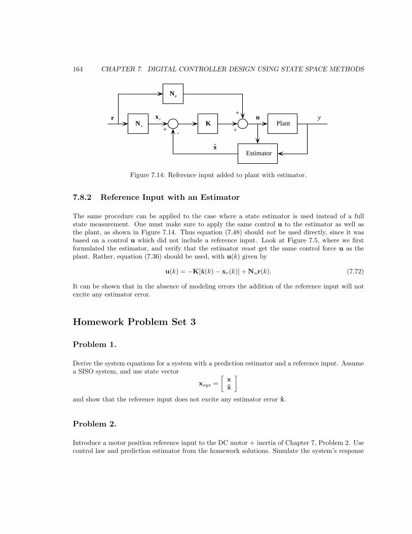
164 CHAPTER 7. DIGITAL CONTROLLER DESIGN USING STATE SPACE METHODS
r x r u
+ - +
+
N x
Nu
K Plant
Estimatorx
y
Figure 7.14: Reference input added to plant with estimator.
7.8.2 Reference Input with an Estimator
The same procedure can be applied to the case where a state estimator is used instead of a fullstate measurement. One must make sure to apply the same control u to the estimator as well asthe plant, as shown in Figure 7.14. Thus equation (7.48) should not be used directly, since it wasbased on a control u which did not include a reference input. Look at Figure 7.5, where we firstformulated the estimator, and verify that the estimator must get the same control force u as theplant. Rather, equation (7.36) should be used, with u(k) given by
u(k) = −K[x(k)− xr(k)] + Nur(k). (7.72)
It can be shown that in the absence of modeling errors the addition of the reference input will notexcite any estimator error.
Homework Problem Set 3
Problem 1.
Derive the system equations for a system with a prediction estimator and a reference input. Assumea SISO system, and use state vector
xsys =
[xx
]and show that the reference input does not excite any estimator error x.
Problem 2.
Introduce a motor position reference input to the DC motor + inertia of Chapter 7, Problem 2. Usecontrol law and prediction estimator from the homework solutions. Simulate the system’s response

7.9. UNIQUENESS OF SOLUTION—THE MIMO CASE 165
to a rest-to-rest load maneuver of 10 degrees in 0.5 sec, where θl(t) is given by a cubic polynomialθl(t) = a0 + a1t + a2t
2 + a3t3. This is a more realistic reference input to track than a step, for
example.
7.9 Uniqueness of Solution—The MIMO Case
The previous approach to the introduction of a reference input is general with respect to the numberof inputs and outputs. However, the solution may not be unique. Consider a system of the followingdimension:
• m plant inputs—u is m× 1
• n states—x is n× 1
• p outputs—yr and r are p× 1
The dimension of equation (7.70) isn×n︷ ︸︸ ︷
Φ− I
n×m︷︸︸︷Γ
Cr︸︷︷︸p×n
0︸︷︷︸p×m
︸ ︷︷ ︸
(n+p)×(n+m)
n×p︷︸︸︷Nx
Nu︸︷︷︸m×p
︸ ︷︷ ︸(n+m)×p
=
n×p︷︸︸︷0I︸︷︷︸p×p
︸ ︷︷ ︸
(n+p)×p
. (7.73)
From equation (7.73) it is clear that if m = p the coefficient matrix is square and may be directlyinverted. However, if m 6= p this is not true. But there is still a solution, there is just not a uniquesolution. The problem is analogous to the classic linear algebra problem Ax = b.
The mathematics of why the following approach works will be treated somewhat in Chapter 8 onSystem Identification. Suffice it to say that we achieve a best least squares fit. When A is notsquare, multiply by AT to get ATAx = ATb. Now ATA may be inverted, and the solution isx = [A
TA]−1ATx. The reference input problem is identical, and if we let[
Φ− I ΓCr 0
]∆= Ψ
the solution when there are differing numbers of plant inputs and controlled outputs is[Nx
Nu
]=[ΨTΨ
]−1ΨT
[0I
](7.74)
The resulting Nx and Nu can then be used with the methods of Section 7.8.

166 CHAPTER 7. DIGITAL CONTROLLER DESIGN USING STATE SPACE METHODS
PositionServo
u
x
θ
lζ , ωn
Figure 7.15: Pendulum and cart driven by position servo.
7.10 Another Example—Stick Balancer
Consider the inverted pendulum on a cart driven by a position servo as shown in Figure 7.15. Theequation of motion of the pendulum is
x+ lθ − gθ = 0
and the cart is
x+ 2ζωnx+ ω2nx = ω2
nu
where u is the input to the position servo.
Eliminate x using both equations of motion, and one gets
θ =g
lθ +
ω2n
lx+
2ζωnl
x− ω2n
lu
Pick the state vector
x =
x1
x2
x3
x4
=
θ
θxx
then the following system and input matrices obtain:
A =
0 1 0 0g/l 0 ω2
n/l 2ζωn/l0 0 0 10 0 −ω2
n −2ζωn
,B =
0
−ω2n/l0ω2n
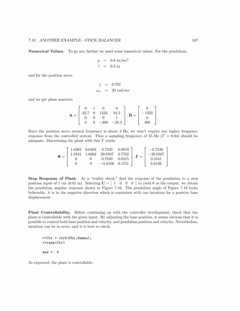
7.10. ANOTHER EXAMPLE—STICK BALANCER 167
Numerical Values. To go any farther we need some numerical values. For the pendulum,
g = 9.8 m/sec2
l = 0.3 m
and for the position servo
ζ = 0.707
ωn = 20 rad/sec
and we get plant matrices
A =
0 1 0 0
32.7 0 1333 94.30 0 0 10 0 −400 −28.3
,B =
0
−13330
400
Since the position servo natural frequency is about 3 Hz, we won’t require any higher frequencyresponse from the controlled system. Thus a sampling frequency of 25 Hz (T = 0.04) should beadequate. Discretizing the plant with this T yields
Φ =
1.0262 0.0403 0.7240 0.06191.3181 1.0262 29.0507 2.7782
0 0 0.7839 0.02150 0 −8.6106 0.1751
,Γ =
−0.7240−29.0507
0.21618.6106
Step Response of Plant. As a “reality check,” find the response of the pendulum to a stepposition input of 1 cm (0.01 m). Selecting C =
[1 0 0 0
]to yield θ as the output, we obtain
the pendulum angular response shown in Figure 7.16. The pendulum angle of Figure 7.16 looksbelievable, it is in the negative direction which is consistent with our intuition for a positive basedisplacement.
Plant Controllability. Before continuing on with the controller development, check that theplant is controllable with the given input. By adjusting the base position, it seems obvious that it ispossible to control both base position and velocity, and pendulum position and velocity. Nevertheless,intuition can be in error, and it is best to check.
>>Ctr = ctrb(Phi,Gamma);
>>rank(Ctr)
ans = 4
As expected, the plant is controllable.

168 CHAPTER 7. DIGITAL CONTROLLER DESIGN USING STATE SPACE METHODS
0 0.2 0.4 0.6 0.8-70
-60
-50
-40
-30
-20
-10
0
time
pend
ulum
ang
le (
degr
ees)
Figure 7.16: Response of pendulum to 1 cm step servo displace-ment.
Control Law. In keeping with Butterworth filter guidelines, equally space four poles at radius ωnaround the negative real axis in the s-plane, hence at angles of ±22.5o,±67.5o from the negativereal axis. Thus the four poles are at s = −7.6537 ± j18.4776, s = −18.4776 ± j7.6537. In the zplane these four poles are z = 0.5442± j0.4960, z = 0.4553± j0.1439.
Using Matlab place, the state feedback gain is
K =[−3.1715 −0.3895 −8.5452 −1.2489
]Plant Observability Assume that only a measurement of pendulum angle is available (measure-ment of cart position is probably available, since its position is controlled), can we estimate the fullstate vector from only a measurement of pendulum angle? The C matrix will be
C =[
1 0 0 0]
and a check of the observability matrix shows
>>C = [1 0 0 0];
>>rank(ctrb(Phi’,C’))
ans = 4
Since the observability matrix O has full rank, the system is observable, and we can proceed with aprediction estimator design.
7.10. ANOTHER EXAMPLE—STICK BALANCER 169
Prediction Estimator Place the estimator poles like the previous control law poles, but use ahigher natural frequency of ωn = 50 rad/sec. These poles are at s = −19.1342 ± j46.1940 ands = −46.1940 ± j19.1342. The corresponding z-plane locations are z = −0.1272 ± j0.4474 andz = 0.1136± j0.1092. Again using the place function, we get
L =
3.038664.3273−0.03205.6954
Reference Input We wish to specify the position of the cart using the reference input, or yr = x.This is a different variable than the measurement θ, so Cr 6= C, and
Cr =[
0 0 1 0]
It doesn’t really make sense to provide a reference input for pendulum angle θ, except for trimming,since θ = 0 is the only pendulum angle that can exist in steady-state. So the number of plant inputsu and desired outputs x are the same (m = p), hence the coefficient matrix in equation (7.70) issquare, and terms Nx and Nu are given by equation (7.71),
>>Cr = [0 0 1 0];
>>inv([Phi-eye(4) Gamma ; Cr 0])*([0;0;0;0;1])
ans = -0.0000
0.0000
1.0000
0.0000
1.0000
Thus
Nx =
0010
, Nu = 1
System Modeling. The complete system is modeled by the five following equations (integratedin the proper manner, of course!):
x(k + 1) = Φx(k) + Γu(k)
y(k) = Cx(k)
x(k + 1) = Φx(k) + Γu(k) + L[y(k)−Cx(k)]
u(k) = −K[x(k)− xr(k)] +Nur(k)
xr(k) = Nxr(k)
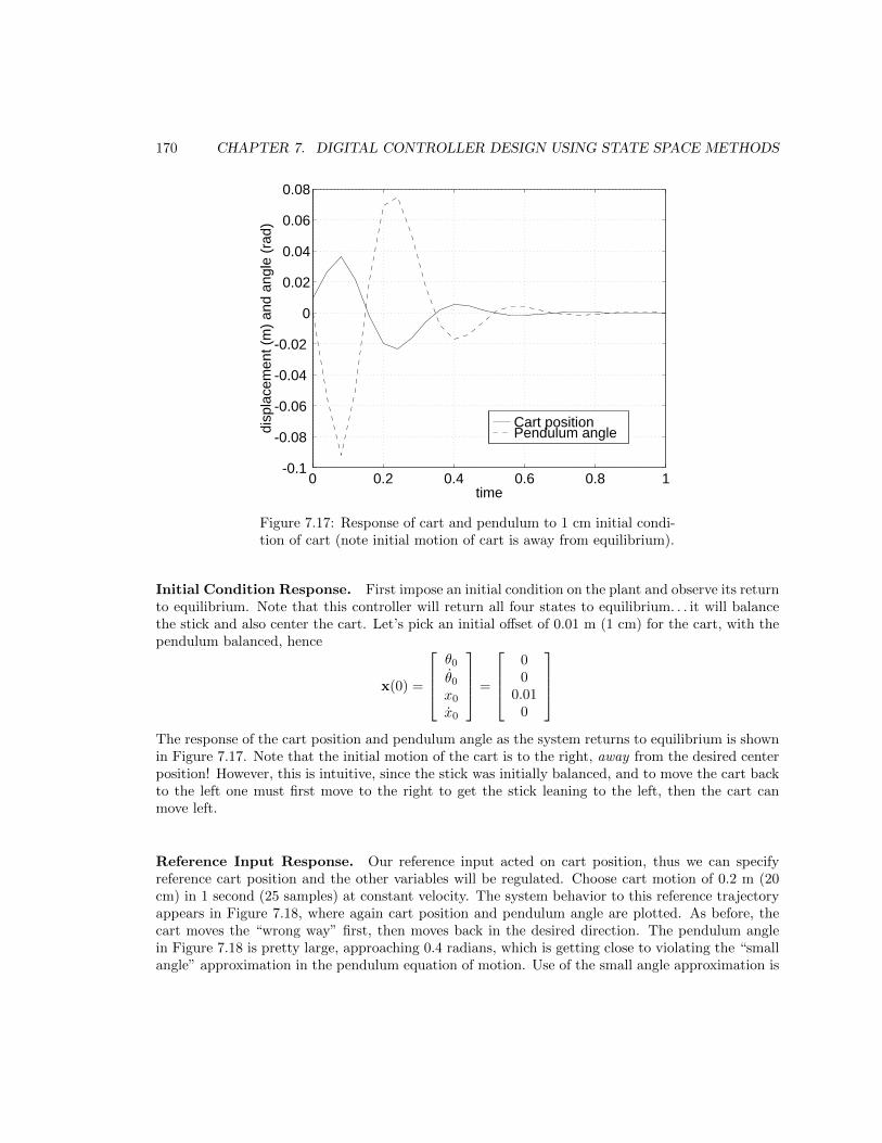
170 CHAPTER 7. DIGITAL CONTROLLER DESIGN USING STATE SPACE METHODS
0 0.2 0.4 0.6 0.8 1-0.1
-0.08
-0.06
-0.04
-0.02
0
0.02
0.04
0.06
0.08
time
disp
lace
men
t (m
) an
d an
gle
(rad
)
Cart position Pendulum angle
Figure 7.17: Response of cart and pendulum to 1 cm initial condi-tion of cart (note initial motion of cart is away from equilibrium).
Initial Condition Response. First impose an initial condition on the plant and observe its returnto equilibrium. Note that this controller will return all four states to equilibrium. . . it will balancethe stick and also center the cart. Let’s pick an initial offset of 0.01 m (1 cm) for the cart, with thependulum balanced, hence
x(0) =
θ0
θ0
x0
x0
=
00
0.010
The response of the cart position and pendulum angle as the system returns to equilibrium is shownin Figure 7.17. Note that the initial motion of the cart is to the right, away from the desired centerposition! However, this is intuitive, since the stick was initially balanced, and to move the cart backto the left one must first move to the right to get the stick leaning to the left, then the cart canmove left.
Reference Input Response. Our reference input acted on cart position, thus we can specifyreference cart position and the other variables will be regulated. Choose cart motion of 0.2 m (20cm) in 1 second (25 samples) at constant velocity. The system behavior to this reference trajectoryappears in Figure 7.18, where again cart position and pendulum angle are plotted. As before, thecart moves the “wrong way” first, then moves back in the desired direction. The pendulum anglein Figure 7.18 is pretty large, approaching 0.4 radians, which is getting close to violating the “smallangle” approximation in the pendulum equation of motion. Use of the small angle approximation is
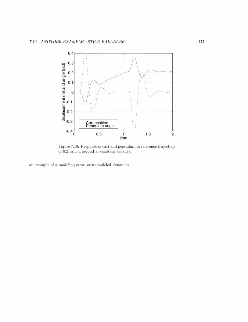
7.10. ANOTHER EXAMPLE—STICK BALANCER 171
0 0.5 1 1.5 2-0.4
-0.3
-0.2
-0.1
0
0.1
0.2
0.3
0.4
time
disp
lace
men
t (m
) an
d an
gle
(rad
)
Cart position Pendulum angle
Figure 7.18: Response of cart and pendulum to reference trajectoryof 0.2 m in 1 second at constant velocity.
an example of a modeling error, or unmodeled dynamics.

172 CHAPTER 7. DIGITAL CONTROLLER DESIGN USING STATE SPACE METHODS

Chapter 8
System Identification
8.1 Introduction
To design a controller for a dynamic system it is necessary to have a model that describes thedynamic behavior of that system. There are fundamentally two approaches to finding this model:
Analytical Modeling Using basic principles. . . the laws of motion, electrical laws, and other phys-ical principles, the designer obtains differential equations of motion describing the response ofmechanical, electrical, thermal, fluid, and other systems.
Experimental Identification Excite the dynamic system with a given input, and record its out-put. Construct a model from this observed data.
While analytical modeling is almost always of some use, if for nothing more than to give insight intothe expected model structure, actual physical phenomena may be too complex to permit satisfactorydescription using physical principles. Under these circumstances, the designer looks to experimentaldata, and experimental system identification.
This chapter will contain a very brief treatment of system identification using the least squaresmethod. We will make the assumption that the system to be identified is linear and time-invariant,in keeping with the prior chapters.
8.2 Models and Data Organization
Let’s use a second-order transform-based discrete system to illustrate the procedure. Consider
Y (z)
U(z)=
b1z−1 + b2z
−2
1− a1z−1 − a2z−2(8.1)
173
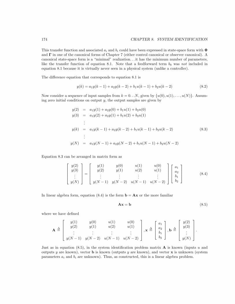
174 CHAPTER 8. SYSTEM IDENTIFICATION
This transfer function and associated ai and bi could have been expressed in state-space form with Φand Γ in one of the canonical forms of Chapter 7 (either control canonical or observer canonical). Acanonical state-space form is a “minimal” realization. . . it has the minimum number of parameters,like the transfer function of equation 8.1. Note that a feedforward term b0 was not included inequation 8.1 because it is virtually never seen in a physical system (unlike a controller).
The difference equation that corresponds to equation 8.1 is
y(k) = a1y(k − 1) + a2y(k − 2) + b1u(k − 1) + b2u(k − 2) (8.2)
Now consider a sequence of input samples from k = 0. . .N , given by u(0), u(1), . . . , u(N). Assum-ing zero initial conditions on output y, the output samples are given by
y(2) = a1y(1) + a2y(0) + b1u(1) + b2u(0)
y(3) = a1y(2) + a2y(1) + b1u(2) + b2u(1)
...
y(k) = a1y(k − 1) + a2y(k − 2) + b1u(k − 1) + b2u(k − 2) (8.3)
...
y(N) = a1y(N − 1) + a2y(N − 2) + b1u(N − 1) + b2u(N − 2)
Equation 8.3 can be arranged in matrix form asy(2)y(3)
...y(N)
=
y(1) y(0) u(1) u(0)y(2) y(1) u(2) u(1)
......
......
y(N − 1) y(N − 2) u(N − 1) u(N − 2)
a1
a2
b1b2
(8.4)
In linear algebra form, equation (8.4) is the form b = Ax or the more familiar
Ax = b (8.5)
where we have defined
A∆=
y(1) y(0) u(1) u(0)y(2) y(1) u(2) u(1)
......
......
y(N − 1) y(N − 2) u(N − 1) u(N − 2)
,x ∆=
a1
a2
b1b2
,b ∆=
y(2)y(3)
...y(N)
.Just as in equation (8.5), in the system identification problem matrix A is known (inputs u andoutputs y are known), vector b is known (outputs y are known), and vector x is unknown (systemparameters ai and bi are unknown). Thus, as constructed, this is a linear algebra problem.
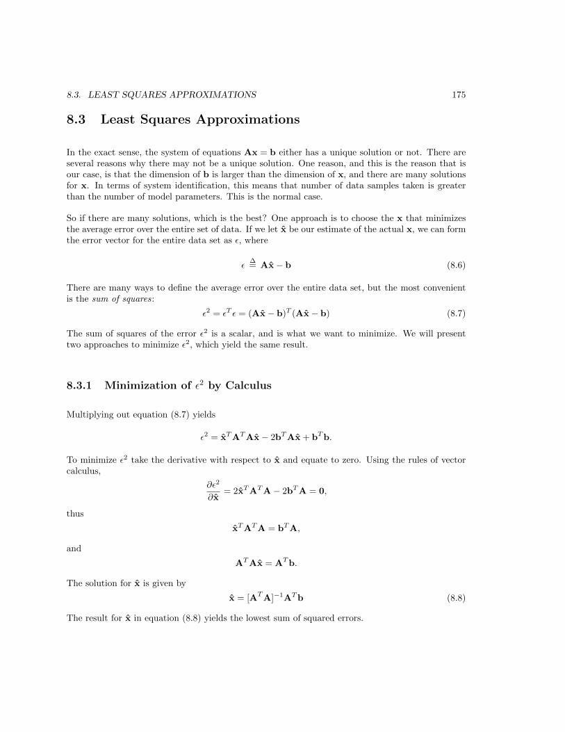
8.3. LEAST SQUARES APPROXIMATIONS 175
8.3 Least Squares Approximations
In the exact sense, the system of equations Ax = b either has a unique solution or not. There areseveral reasons why there may not be a unique solution. One reason, and this is the reason that isour case, is that the dimension of b is larger than the dimension of x, and there are many solutionsfor x. In terms of system identification, this means that number of data samples taken is greaterthan the number of model parameters. This is the normal case.
So if there are many solutions, which is the best? One approach is to choose the x that minimizesthe average error over the entire set of data. If we let x be our estimate of the actual x, we can formthe error vector for the entire data set as ε, where
ε∆= Ax− b (8.6)
There are many ways to define the average error over the entire data set, but the most convenientis the sum of squares:
ε2 = εT ε = (Ax− b)T (Ax− b) (8.7)
The sum of squares of the error ε2 is a scalar, and is what we want to minimize. We will presenttwo approaches to minimize ε2, which yield the same result.
8.3.1 Minimization of ε2 by Calculus
Multiplying out equation (8.7) yields
ε2 = xTATAx− 2bTAx + bTb.
To minimize ε2 take the derivative with respect to x and equate to zero. Using the rules of vectorcalculus,
∂ε2
∂x= 2xTATA− 2bTA = 0,
thus
xTATA = bTA,
and
ATAx = ATb.
The solution for x is given by
x = [ATA]−1ATb (8.8)
The result for x in equation (8.8) yields the lowest sum of squared errors.
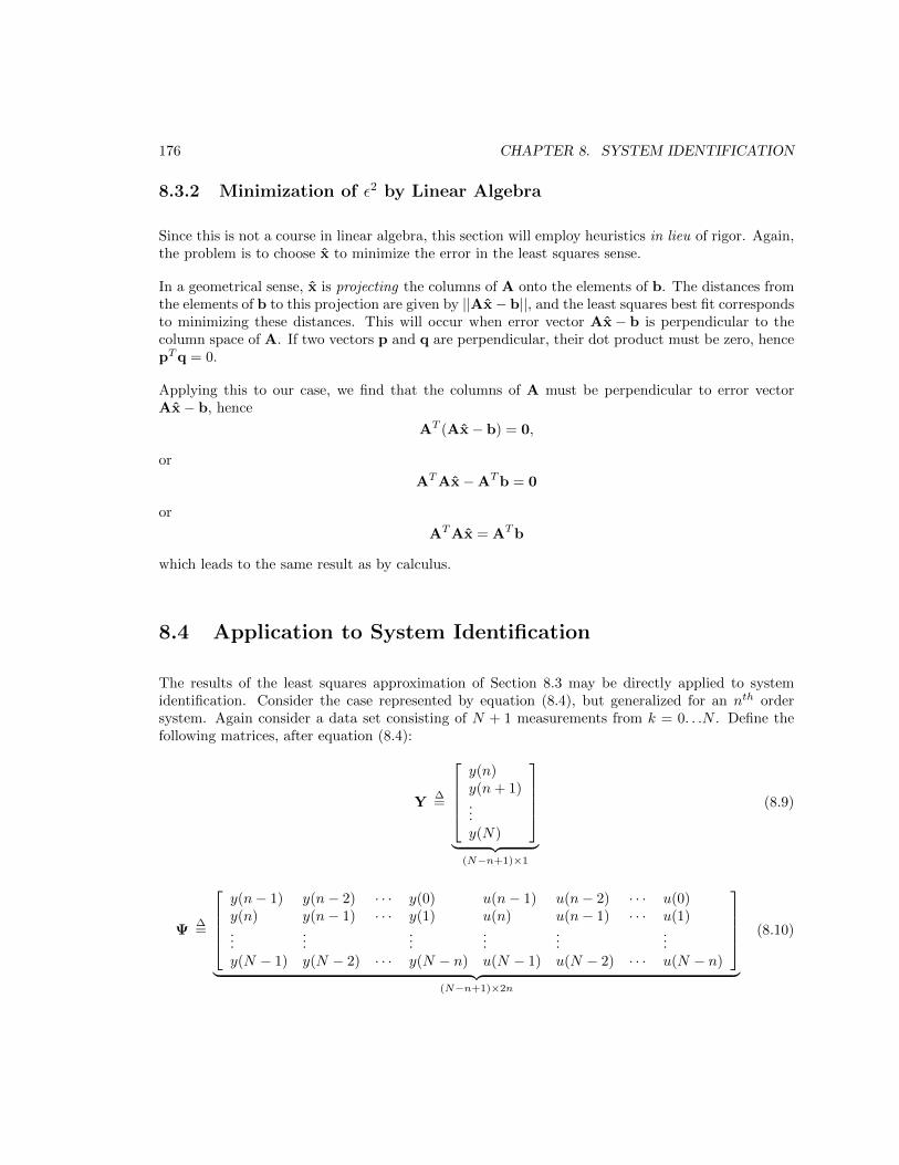
176 CHAPTER 8. SYSTEM IDENTIFICATION
8.3.2 Minimization of ε2 by Linear Algebra
Since this is not a course in linear algebra, this section will employ heuristics in lieu of rigor. Again,the problem is to choose x to minimize the error in the least squares sense.
In a geometrical sense, x is projecting the columns of A onto the elements of b. The distances fromthe elements of b to this projection are given by ||Ax− b||, and the least squares best fit correspondsto minimizing these distances. This will occur when error vector Ax− b is perpendicular to thecolumn space of A. If two vectors p and q are perpendicular, their dot product must be zero, hencepTq = 0.
Applying this to our case, we find that the columns of A must be perpendicular to error vectorAx− b, hence
AT (Ax− b) = 0,
or
ATAx−ATb = 0
or
ATAx = ATb
which leads to the same result as by calculus.
8.4 Application to System Identification
The results of the least squares approximation of Section 8.3 may be directly applied to systemidentification. Consider the case represented by equation (8.4), but generalized for an nth ordersystem. Again consider a data set consisting of N + 1 measurements from k = 0. . .N . Define thefollowing matrices, after equation (8.4):
Y∆=
y(n)y(n+ 1)...y(N)
︸ ︷︷ ︸
(N−n+1)×1
(8.9)
Ψ∆=
y(n− 1) y(n− 2) · · · y(0) u(n− 1) u(n− 2) · · · u(0)y(n) y(n− 1) · · · y(1) u(n) u(n− 1) · · · u(1)...
......
......
...y(N − 1) y(N − 2) · · · y(N − n) u(N − 1) u(N − 2) · · · u(N − n)
︸ ︷︷ ︸
(N−n+1)×2n
(8.10)

8.5. PRACTICAL ISSUES—HOW WELL DOES IT WORK? 177
Θ∆=
a1
a2
· · ·anb1b2· · ·bn
︸ ︷︷ ︸
2n×1
(8.11)
With the definitions of (8.9), (8.10), and (8.11), the equation describing the input-output data andmodel parameters may be written as
Y = ΨΘ (8.12)
which is exactly in the form of b = Ax. Thus the development of Section 8.3 is directly applicable,and the solution for the model parameter vector Θ is
Θ = [ΨTΨ]−1ΨTY. (8.13)
Equation (8.13) yields the best fit in the least squares sense.
Note that the order of the model is up to the designer. Selection of the order should be based onphysical reasoning. Of course, the designer may perform multiple fits with different orders and selectthe lowest order fit that yields acceptable agreement. Selecting a model of too-high order meansthat you use the “extra” parameters to fit noise in the data. And remember that there is alwaysquantization noise.
8.5 Practical Issues—How Well Does it Work?
Least squares is the simplest and most straightforward parametric identification method. If thesystem to be identified exhibits linear behavior and the input/output data is relatively noise-free,least squares will yield acceptable results. There are a host of more sophisticated methods thatwork better than least squares under more difficult conditions, but they are beyond the scope of thisbook.
8.5.1 Selection of Input
The choice of input u used in identification is important. Examine equations (8.3) for a moment, inparticular the input terms involving u(k) and bi. Consider the (absurd) case where the input u(k)was a constant. Then in each equation in (8.3) the bi terms would be multiplied by the same number,and would be combined into a single quantity. We could not ever separate the bi terms from theobserved data. The constant u fails to “excite” all the dynamics of the plant. This problem has beenstudied extensively, and an input sequence u(k) that fluctuates enough to avoid the possibility oflinear combinations of the elements of model parameter vector Θ showing up in the error is calledpersistently exciting.

178 CHAPTER 8. SYSTEM IDENTIFICATION
Two types of inputs will be shown in this section:
• Random Input
• Random Binary Input
Random Input. This is just random noise, which may be easily generated using MATLAB. Ifrandom the harmonic content will be rich enough to be persistently exciting. Either a normal oruniform distribution is available. A normal distribution with mean of 0.0 and variance 1.0 may becreated with the randn function. A plot of a such a normal distribution for k = 0. . .100 is shown inFigure 8.1. Naturally the random input may have to be biased and scaled before application to agiven physical system.
Random Binary Input This is a random input that fluctuates between two distinct values. Itis a series of pulses with random durations. Since a step signal has infinite harmonic content, thistype of input will also persistently excite the system. A random binary input is shown in Figure 8.2
Both types of random inputs may be easily generated using the MATLAB randn (normally-distributedrandom sequence) function, along with the sign function for producing the binary signal.
8.5.2 Quantization Noise
As briefly discussed in Section 1.2, quantization effects are always present whenever there is aconversion between the analog and digitial domains. The size of the quantum is dependent on therange and resolution of the conversion device. For example, an 8-bit A/D converter digitizes to1 part in 256. If the A/D has a range of ±5V, the voltage quantum is q = 10/256 = 0.0391 V.Depending on how close the analog voltage is to one of the levels of quantization, there will be moreor less quantization error present. Note that in identification, quantization only affects output y,since the input u is already quantized when it is acquired by the computer.
Quantization can be either rounding or truncation. A plot of the effect of rounding is shown inFigure 8.3. In Figure 8.3, if the input is between ±0.5, the output is zero. If the input is between 0.5and 1.5, the output is 1, and so on. The quantization error fluctuates between ±q in a “sawtooth”variation.
The amount of quantization noise is also dependent on how well we use the full range of the conversiondevice. If our input is only ±1 V, and the A/D has a range of ±5 V, the effective resolution will beless than the possible resolution. If possible, the full range of conversion devices should be used.
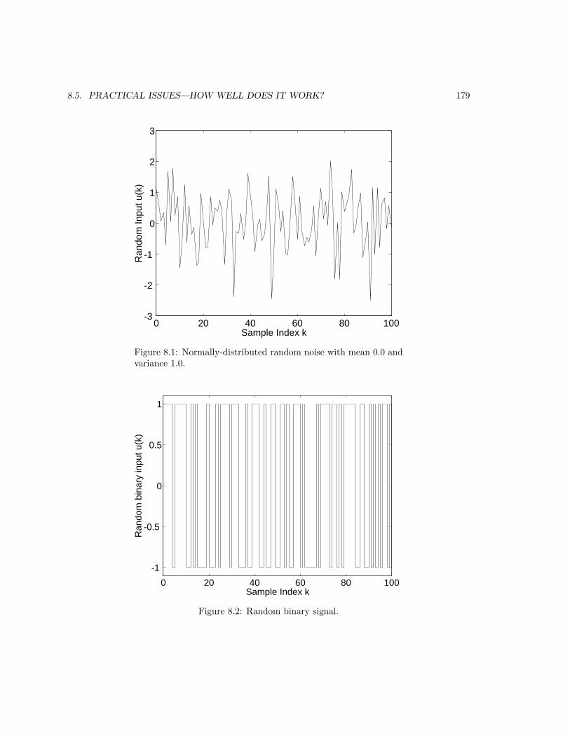
8.5. PRACTICAL ISSUES—HOW WELL DOES IT WORK? 179
0 20 40 60 80 100-3
-2
-1
0
1
2
3
Sample Index k
Ran
dom
Inpu
t u(k
)
Figure 8.1: Normally-distributed random noise with mean 0.0 andvariance 1.0.
0 20 40 60 80 100
-1
-0.5
0
0.5
1
Sample Index k
Ran
dom
bin
ary
inpu
t u(k
)
Figure 8.2: Random binary signal.

180 CHAPTER 8. SYSTEM IDENTIFICATION
-10 -5 0 5 10-10
-5
0
5
10
Input
Qua
ntiz
ed O
utpu
t
Figure 8.3: Effect of rounding with q = 1.
8.5.3 Identification Example
As an example, consider the third order continuous system with transfer function
G(s) =2000
(s+ 10)(s2 + 20s+ 200)=
2000
(s+ 10)(s+ 10± j10)
The complex poles have natural frequency ωn ≈ 14 rad/sec, or about 2.25 Hz, so pick samplingfrequency of 20 Hz, or T = 0.05 sec. Preceding this G(s) by a sampler and following it by a ZOH(our standard discretization procedure) yields its discrete form,
G(z) =0.0284z−1 + 0.0775z−2 + 0.0134z−3
1− 1.6711z−1 + 1.0136z−2 − 0.2231z−3=
0.0284(z + 0.1857)(z + 2.54)
(z − 0.6065)(z − 0.5323± j0.2908)
Excitation. Excite this G(z) with 101 samples of a random binary signal of amplitude ±1 asshown in Figure 8.2. Assume that the output is quantized by an A/D with 8-bit resolution and ±5Vrange.
The quantized response of this system is shown in Figure 8.4.
Least-Squares Fit. The input data u(k) and output data y(k) must be arranged according toequations (8.9) and (8.10) to form the Y and Ψ matrices, then the least-squares solution for modelparameter vector Θ is given by equation (8.13). Here N = 100 and n = 3, and Y and Ψ areconstructed accordingly.

8.5. PRACTICAL ISSUES—HOW WELL DOES IT WORK? 181
0 20 40 60 80 100-1
-0.8
-0.6
-0.4
-0.2
0
0.2
0.4
0.6
0.8
Sample index k
Out
put y
(k)
Figure 8.4: Quantized output of example G(z) driven by randombinary signal.
Executing this yields model parameter vector
Θ =[
1.4067 −0.5852 0.0192 0.0302 0.0865 0.0284]T
and corresponding estimated transfer function
G(z) =0.0302z−1 + 0.0865z−2 + 0.0284z−3
1− 1.4067z−1 + 0.5852z−2 − 0.0192z−3=
0.0302(z + 0.3784)(z + 2.4894)
(z − 0.0358)(z − 0.6855± j0.2574)
Step Response. How does the step response of the model compare with the actual system? Bothunit step responses are shown in Figure 8.5. While the steady-state value is somewhat inaccurate,the transient portion of the response exhibits excellent agreement.
Comments. In this example, we did not make good use of the range of the A/D converter, using
only about ±1V range of the ±5V converter. This contributed to the inaccuracy. Even so, the G(z)we obtained would serve pretty well for controller design.
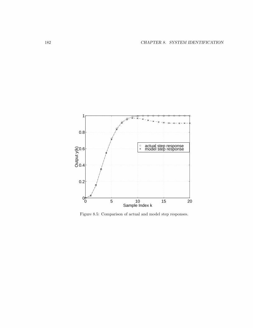
182 CHAPTER 8. SYSTEM IDENTIFICATION
0 5 10 15 200
0.2
0.4
0.6
0.8
1
Sample Index k
Out
put y
(k) actual step response
model step response
Figure 8.5: Comparison of actual and model step responses.

8.5. PRACTICAL ISSUES—HOW WELL DOES IT WORK? 183
Homework Problems
Problem 1.
Data from a mass moving in a plane (x, y) without force are given below. Plot the points and use
t x y
0 -0.426 1.5011 0.884 1.7772 2.414 2.5303 2.964 3.4414 3.550 3.7625 5.270 4.3286 5.625 4.0167 7.188 5.3688 8.129 5.7369 9.225 6.49910 10.388 6.233
least squares to estimate the initial value of x, the initial value of y, and the velocity of the mass inx and y. Draw the curve (line) that corresponds to your estimates.
Problem 2.
Select a discrete transfer function (at least second order) and investigate identifying its parameters.
(a) Drive the system with both random and PRBS inputs.
(b) Perform least-square fits both using a model structure that is the correct order, and an ordergreater than the “actual” order.
(c) What happens when the model order is too high?