Embed Size (px)
Citation preview

Lecture NotesIntroduction to Black Hole Astrophysics, 2010Gustavo E. Romero
Introduction to black hole astrophysics
Gustavo E. RomeroInstituto Argentino de Radioastronomía, C.C. 5, Villa Elisa (1894), andFacultad de Cs. Astronómicas y Geofísicas, UNLP, Paseo del BosqueS/N, (1900) La Plata, Argentina, [email protected]
Es cosa averiguada que no se sabe nada,y que todos son ignorantes;
y aun esto no se sabe de cierto,que, a saberse, ya se supiera algo: sospéchase.
Quevedo
Abstract. Black holes are perhaps the most strange and fascinatingobjects in the universe. Our understanding of space and time is pushedto its limits by the extreme conditions found in these objects. Theycan be used as natural laboratories to test the behavior of matter invery strong gravitational fields. Black holes seem to play a key role inthe universe, powering a wide variety of phenomena, from X-ray binariesto active galactic nuclei. In these lecture notes the basics of black holephysics and astrophysics are reviewed.
1. Introduction
Strictly speaking, black holes do not exist. Moreover, holes, of any kind, do notexist. You can talk about holes of course. For instance you can say: “there isa hole in the wall”. You can give many details of the hole: it is big, it is roundshaped, light comes in through it. Even, perhaps, the hole could be such thatyou can go through to the outside. But I am sure that you do not think thatthere is a thing made out of nothingness in the wall. No. To talk about thehole is an indirect way of talking about the wall. What really exists is the wall.The wall is made out of bricks, atoms, protons and leptons, whatever. To saythat there is a hole in the wall is just to say that the wall has certain topology,a topology such that not every closed curve on the surface of the wall can becontracted to a single point. The hole is not a thing. The hole is a property ofthe wall.
Let us come back to black holes. What are we talking about when we talkabout black holes?. Space-time. What is space-time?.
Space-time is the ontological sum of all events of all things.
1
2 Gustavo E. Romero
A thing is an individual endowed with physical properties. An event is achange in the properties of a thing. An ontological sum is an aggregation ofthings or physical properties, i.e. a physical entity or an emergent property.An ontological sum should not be confused with a set, which is a mathematicalconstruct and has only mathematical (i.e. fictional) properties.
Everything that has happened, everything that happens, everything thatwill happen, is just an element, a “point”, of space-time. Space-time is not athing, it is just the relational property of all things1.
As it happens with every physical property, we can represent space-timewith some mathematical structure, in order to describe it. We shall adopt thefollowing mathematical structure for space-time:
Space-time can be represented by a C∞-differentiable, 4-dimensional, realmanifold.
A real 4-D manifold is a set that can be covered completely by subsets whoseelements are in a one-to-one correspondence with subsets of �4. Each elementof the manifold represents an event. We adopt 4 dimensions because it seemsenough to give 4 real numbers to localize an event. For instance, a lightning hasbeaten the top of the building, located in the 38th Av., between streets 20 and21, at 25 m above the see level, La Plata city, at 4:35 am, local time, March 2nd,2009 (this is my home at the time of writing). We see now why we choose amanifold to represent space-time: we can always provide a set of 4 real numbersfor every event, and this can be done independently of the intrinsic geometry ofthe manifold. If there is more than a single characterization of an event, we canalways find a transformation law between the different coordinate systems. Thisis a basic property of manifolds.
Now, if we want to calculate distances between two events, we need morestructure on our manifold: we need a geometric structure. We can get thisintroducing a metric tensor that allows to calculate distances. For instance,consider an Euclidean metric tensor δμν (indices run from 0 to 3):
δμν =
⎛⎜⎜⎝1 0 0 00 1 0 00 0 1 00 0 0 1
⎞⎟⎟⎠ . (1)
Then, adopting the Einstein convention of sum, we have that the distanceds between two arbitrarily close events is:
ds2 = δμνdxμdxν = (dx0)2 + (dx1)2 + (dx3)2 + (dx3)2. (2)
Restricted to 3 coordinates, this is the way distances have been calculated sincePythagoras. The world, however, seems to be a little more complicated. After theintroduction of the Special Theory of Relativity by Einstein (1905), the Germanmathematician Hermann Minkowski introduced the following pseudo-Euclideanmetric which is consistent with Einstein’s theory (Minkowski 1907, 1909):
1For more details on this view see Perez-Bergliaffa et al. (1998).

Black hole astrophysics 3
t 1
2
3
t
t
t t t2 31
300000 km
1 se
c
Space
Spac
e
Tim
e
light
forbidden
mat
ter
(a) Spatial representation (b) The light cone
Figure 1Figure 1. Light cone. From J-P. Luminet (1998).
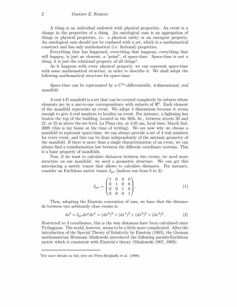
ds2 = ημνdxμdxν = (dx0)2 − (dx1)2 − (dx3)2 − (dx3)2. (3)
The Minkowski metric tensor ημν has rank 2 and trace −2. We call thecoordinates with the same sign spatial (adopting the convention x1 = x, x2 = y,and x3 = z) and the coordinate x0 = ct is called temporal coordinate. Theconstant c is introduced to make uniform the units. There is an important factrespect to Eq. (3): contrary to what was thought by Kant and others, it isnot a necessary statement. Things might have been different. We can easilyimagine possible worlds with other metrics. This means that the metric tensorhas empirical information about the real universe.
Once we have introduced a metric tensor we can separate space-time at eachpoint in three regions according to ds2 < 0 (space-like region), ds2 = 0 (light-like or null region), and ds2 > 0 (time-like region). Particles that go throughthe origin can only reach time-like regions. The null surface ds2 = 0 can beinhabited only by particles moving at the speed of light, like photons. Points inthe space-like region cannot be reached by material objects from the origin ofthe light cone that can be formed at any space-time point.
The introduction of the metric allows to define the future and the past of agiven event. Once this is done, all events can be classified by the relation “earlierthan” or “later than”. The selection of “present” event - or “now” - is entirelyconventional. To be present is not an intrinsic property of any event. Rather,it is a secondary, relational property that requires interaction with a consciousbeing. The extinction of the dinosaurs will always be earlier than the beginningof World War II. But the latter was present only to some human beings at somephysical state. The present is a property like a scent or a color. It emergesfrom the interaction of self-conscious individuals with changing things and hasnot existence independently of them (for more about this, see Grünbaum 1973,Chapter X).
Let us consider the unitary vector T ν = (1, 0, 0, 0), then a vector xμ pointsto the future if ημνxμT ν > 0. In the similar way, the vector points toward thepast if ημνxμT ν < 0. A light cone is shown in Figure 1.
4 Gustavo E. Romero
We define the proper time (τ) of a physical system as the time of a co-movingsystem, i.e. dx = dy = dz = 0, and hence:
dτ2 =1
c2ds2. (4)
Since the interval is an invariant (i.e. it has the same value in all coordinatesystems), it is easy to show that:
dτ =dt
γ, (5)
whereγ =
1√1− (v
c
)2 (6)
is the Lorentz factor of the system.A basic characteristic of Minskowski space-time is that it is “flat”: all light
cones point in the same direction, i.e. the local direction of the future doesnot depend on the coefficients of the metric since these are constants. Moregeneral space-times are possible. If we want to describe gravity in the frameworkof space-time, we have to introduce a pseudo-Riemannian space-time, whosemetric can be flexible, i.e. a function of the material properties (mass-energyand momentum) of the physical systems that produce the events of space-time.
Tetrads: othogonal unit vector fields
Let us consider a scalar product
�v • �w = (vμeμ) • (wν eν) = (eμ • eν)vμwν = gμνvμwν ,
whereeμ = lim
δxμ→0
δ�s
δxμ,
and we have definedeμ(x) • eν(x) = gμν(x).
Similarly,eμ(x) • eν(x) = gμν(x).
We call eμ a coordinate basis vector or a tetrad. δ�s is an infinitesimaldisplacement vector between a point P on the manifold (see Fig. 2) and a nearbypoint Q whose coordinate separation is δxμ along the xμ coordinate curve. eμ isthe tangent vector to the xμ curve at P . We can write:
d�s = eμdxμ
and then:
ds2 = d�s • d�s = (dxμeμ) • (dxν eν) = (eμ • eν)dxμdxν = gμνdxμdxν .
Black hole astrophysics 5
At a given point P the manifold is flat, so:
gμν(P ) = ημν .
A manifold with such a property is called pseudo-Riemannian. If gμν(P ) = δμνthe manifold is called strictly Riemannian.
The basis is called orthonormal when eμ • eν = ημν at any given point P .Notice that since the tetrads are 4-dimensional we can write:
eμa(x)eaν(x) = gμν(x),
andeμa(P )e
aν(P ) = ημν .
The tetrads can vary along a given world-line, but always satisfying:
eμa(τ)eaν(τ) = ημν .
We can also express the scalar product �v • �w in the following ways:
�v • �w = (vμeμ) • (wν e
ν) = (eμ • eν)vμwν = gμνvμwν ,
�v • �w = (vμeμ) • (wν eν) = (eμ • eν)vμwν = vμwνδ
νμ = vμwμ,
and�v • �w = (vμe
μ) • (wν eν) = (eμ • eν)vμwν = δμν vμwν = vμw
μ.
By comparing these expressions for the scalar product of two vectors, wesee that
gμνwν = wμ,
so the quantities gμν can be used to lower and index. Similarly,
gμνwν = wμ.
We also have that
gμνwνgμνwν = gμνg
μνwνwν = wμwμ.
And from here it follows:gμνgμσ = δνσ.
The tensor field gμν(x) is called the metric tensor of the manifold. Alterna-tive, the metric of the manifold can be specified by the tetrads eaμ(x).
2. Gravitation
The key to relate space-time to gravitation is the equivalence principle introducedby Einstein (1907):
At every space-time point in an arbitrary gravitational field itis possible to choose a locally inertial coordinate system such that,within a sufficiently small region of the point in question, the laws ofnature take the same form as in unaccelerated Cartesian coordinatesystems in absence of gravitation (fromulation by Weinberg 1972).
6 Gustavo E. Romero
p
manifold
M
Tp
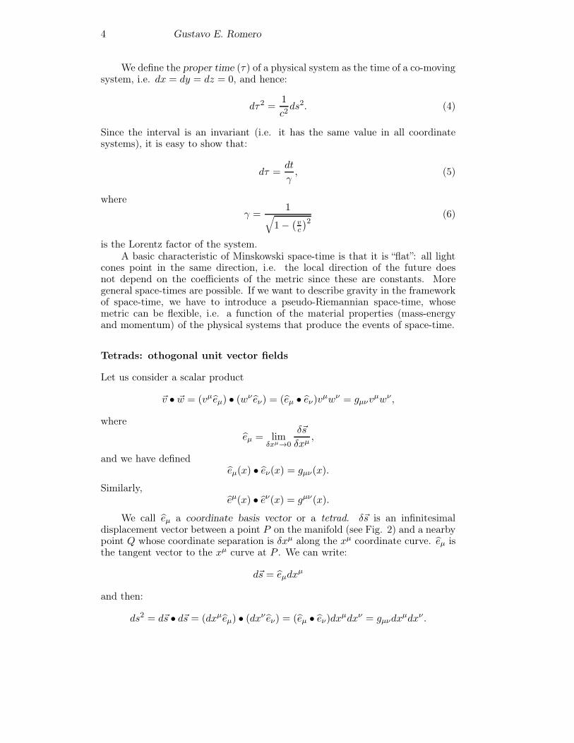
Figure 2. Tangent flat space at a point P of a curved manifold. FromCarroll (2003).
This is equivalent to state that at every point P of the manifold that representsspace-time there is a flat tangent surface. Einstein called the idea that gravitationvanishes in free-falling systems “the happiest thought of my life” (Pais 1982).
In order to introduce gravitation in a general space-time, we define a met-ric tensor gμν , such that its components can be related to those of a locallyMinkowski space-time defined by ds2 = ηαβdξ
αdξβ through a general transfor-mation:
ds2 = ηαβ∂ξα
∂xμ∂ξβ
∂xνdxμdxν = gμνdx
μdxν . (7)
In the absence of gravity we can always find a global coordinate system(ξα) for which the metric can take the form given by Eq. (3) everywhere. Withgravity, on the contrary, such a coordinate system can represent space-time onlyin an infinitesimal neighborhood of a given point. This situation is representedin Fig 2, where the tangent flat space to a point P of the manifold is shown. Thecurvature of space-time means that it is not possible to find coordinates in whichgμν = ημν at all points of the manifold. However, it is always possible to representthe event (point) P in a system such that gμν(P ) = ημν and (∂gμν/∂x
σ)P = 0.To find the equation of motion of a free particle (i.e. only subject to gravity)
in a general space-time of metric gμν let us consider a freely falling coordinatesystem ξα. In such a system:
d2ξα
ds2= 0, (8)
where ds2 = (cdτ)2 = ηαβdξαdξβ. Let us consider now any other coordinate
system xμ. Then,
d
ds
(∂ξα
∂xμdxμ
ds
)= 0 (9)
∂ξα
∂xμd2xμ
ds2+
∂2ξα
∂xμ∂xνdxμ
ds
dxν
ds= 0. (10)
Black hole astrophysics 7
Multiplying at both sides by ∂xλ/∂ξα and using:
∂ξα
∂xμ∂xλ
∂ξα= δλμ, (11)
we getd2xλ
ds2+ Γλ
μν
dxμ
ds
dxν
ds= 0, (12)
where Γλμν is the affine connection of the manifold:
Γλμν ≡ ∂xλ
∂ξα∂2ξα
∂xμ∂xν. (13)
The affine connection can be expressed in terms of derivatives of the metrictensor (see, e.g., Weinberg 1972):
Γλμν =
1
2gλα(∂μgνα + ∂νgμα − ∂αgμν). (14)
Here we use the convention: ∂νf = ∂f/∂xν and gμαgαν = δμν . Notice thatunder a coordinate transformation from xμ to x
′μ the affine connection is nottransformed as a tensor, despite that the metric gμν is a tensor of second rank.
The coefficients Γλμν are said to define a connection on the manifold. ăWhat
are connected are the tangent spaces at different points of the manifold. It isthen possible to compare a vector in the tangent space at point P with thevector parallel to it at another point Q. There is some degree of freedom in thespecification of the affine connection, so we demand symmetry in the last twoindices:
Γλμν = Γλ
νμ
orΓλ[μν] = 0.
In general space-times this requirement is not necessary, and a tensor can beintroduced such that:
T λμν = Γλ
[μν]. (15)
This tensor represents the torsion of space-time. In general relativity space-time is always considered as torsionless, but in the so-called teleparallel theoryof gravity (e.g. Arcos and Pereira 2004) torsion represents the gravitational fieldinstead of curvature, which is nil.
In a pseudo-Riemannian space-time the usual partial derivative is not ameaningful quantity since we can give it different values through different choicesof coordinates. This can be seen in the way the derivative transforms under acoordinate change:
A′μ,ν =
∂
∂x′ν∂x′μ
∂xμAμ =
∂x′μ
∂xμ∂xν
∂x′νAμ
,ν +∂2x′μ
∂xμ∂xν∂xν
∂x′νAμ. (16)
We can define a covariant differentiation through the condition of paralleltransport:
Aμ;ν =∂Aμ
∂xν− Γλ
μνAλ. (17)
8 Gustavo E. Romero
A useful, alternative notation, is:
∇νAμ =∂Aμ
∂xν− Γλ
μνAλ. (18)
A covariant derivative of a vector field is a rank 2 tensor of type (1, 1). Acovariant divergence of a vector field yields a scalar field:
∇μAμ = ∂μA
μ(x)− ΓμαμA
α(x) = φ(x). (19)
A tangent vector satisfies V νVν ;μ= 0. If there is a vector ζμ pointing inthe direction of a symmetry of space-time, then it can be shown (e.g. Weinberg1972):
ζμ;ν +ζν ;μ= 0, (20)
or∇νζμ +∇μζν = 0. (21)
This equation is called Killing’s equation. A vector field ζμ satisfying sucha relation is called a Killing vector.
If there is a curve γ on the manifold, such that its tangent vector is uα =dxα/dλ and a vector field Aα is defined in a neighborhood of γ, we can define aderivative of Aα along γ as:
�μAα = Aα
,βuβ − uα,βA
β = Aα;βu
β − uα;βAβ. (22)
This derivative is a tensor, and it is usually called Lie derivative. It can bedefined for tensor of any type. A Killing vector field is such that:
�ζgμν = 0. (23)
From Eq. (12) we can recover the classical Newtonian equations if:
Γ0i,j = 0, Γi
0,j = 0, Γi0,0 =
∂Φ
∂xi,
where i, j = 1, 2, 3 and Φ is the Newtonian gravitational potential. Then:
x0 = ct = cτ,
d2xi
dτ2= − ∂Φ
∂xi.
We see, then, that the metric represents the gravitational potential and the affineconnection the gravitational field.
The presence of gravity is indicated by the curvature of space-time. TheRiemann tensor, or curvature tensor, provides a measure of this curvature:
Rσμνλ = Γσ
μλ,ν − Γσμν,λ + Γσ
ανΓαμλ − Γσ
αλΓαμν . (24)
The form of the Riemann tensor for an affine-connected manifold can beobtained through a coordinate transformation xμ → xμ that makes the affineconnection to vanish everywhere, i.e.
Γσμν(x) = 0, ∀x, ρ, μ, ν. (25)
Black hole astrophysics 9
The coordinate system xμ exists iff:
Γσμλ,ν − Γσ
μν,λ + ΓσανΓ
αμλ − Γσ
αλΓαμν = 0, (26)
for the affine connection Γσμν(x). The right hand side of Eq. (26) is the Riemann
tensor: Rσμνλ. In such a case the metric is flat, since its derivatives are zero. If
Rσμνλ > 0 the metric has a positive curvature.
The Ricci tensor is defined by:
Rμν = gλσRλμσν = Rσμσν . (27)
Finally, the Ricci scalar is R = gμνRμν .
3. Field equations
The key issue to determine the geometric structure of space-time, and henceto specify the effects of gravity, is to find the law that fixes the metric oncethe source of the gravitational field is given. The source of the gravitationalfield is the energy-momentum tensor Tμν that represents the physical propertiesof a material thing. This was Einstein’s fundamental intuition: the curvatureof space-time at any event is related to the energy-momentum content at thatevent. For the simple case of a perfect fluid the energy-momentum tensor takesthe form:
Tμν = (ε+ p)uμuν − pgμν , (28)
where ε is the mass-energy density, p is the pressure, and uμ = dxμ/ds is the4-velocity. The field equations were found by Einstein (1915) and independentlyby Hilbert (1915) on November 25th and 20th, 1915, respectively2.
We can write Einstein’s physical intuition in the following form:
Kμν = κTμν , (29)
where Kμν is a rank-2 tensor related to the curvature of space-time and κ is aconstant. Since the curvature is expressed by Rμνσρ, Kμν must be constructedfrom this tensor and the metric tensor gμν . The tensor Kμν has the followingproperties to satisfy: i) the Newtonian limit suggests that it should contain termsno higher than linear in the second-order of derivatives of the metric tensor (since∇2Φ = 4πGρ); ii) since Tμν is symmetric then Kμν must be symmetric as well.Since Rμνσρ is already linear in the second-order derivatives of the metric, themost general form of Kμν is:
Kμν = aRμν + bRgμν + λgμν , (30)
where a, b, and λ are constants.
2Recent scholarship has arrived to the conclusion that Einstein was the first to find the equationsand that Hilbert incorporated the final form of the equations in the proof reading process, afterEinstein’s communication (Corry et al. 1997).
10 Gustavo E. Romero
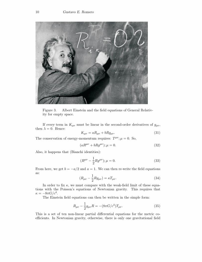
Figure 3. Albert Einstein and the field equations of General Relativ-ity for empty space.
If every term in Kμν must be linear in the second-order derivatives of gμν ,then λ = 0. Hence:
Kμν = aRμν + bRgμν . (31)
The conservation of energy-momentum requires: T μν ;μ = 0. So,
(aRμν + bRgμν);μ = 0. (32)
Also, it happens that (Bianchi identities):
(Rμν − 1
2Rgμν);μ = 0. (33)
From here, we get b = −a/2 and a = 1. We can then re-write the field equationsas:
(Rμν − 1
2Rgμν) = κTμν . (34)
In order to fix κ, we must compare with the weak-field limit of these equa-tions with the Poisson’s equations of Newtonian gravity. This requires thatκ = −8πG/c4.
The Einstein field equations can then be written in the simple form:
Rμν − 1
2gμνR = −(8πG/c4)Tμν . (35)
This is a set of ten non-linear partial differential equations for the metric co-efficients. In Newtonian gravity, otherwise, there is only one gravitational field
Black hole astrophysics 11
equation. General Relativity involves numerous non-linear differential equations.In this fact lays its complexity, and its richness.
The conservation of mass-energy and momentum can be derived from thefield equations:
T μν ;ν = 0 or ∇νTμν = 0. (36)
Contrary to classical electrodynamics, here the field equations entail the energy-momentum conservation and the equations of motion for free particles (i.e. forparticles moving in the gravitational field, treated here as a background pseudo-Riemannian space-time).
Let us consider, for example, a distribution of dust (i.e. a pressureless perfectfluid) for which the energy-momentum tensor is:
T μν = ρuμuν , (37)
with uμ the 4-velocity. Then,
T μν ;μ= (ρuμuν);μ= (ρuμ);μ uν + ρuμuν ;μ= 0. (38)
Contracting with uν :c2(ρuμ);μ+(ρuμ)uνu
ν ;μ= 0, (39)where we used uνuν = c2. Since the second term on the left is zero, we have:
(ρuμ);μ= 0. (40)
Replacing in Eq. (38), we obtain:
uμuν ;ν = 0, (41)
which is the equation of motion for the dust distribution in the gravitationalfield.
Einstein equations (35) can be cast in the form:
Rμν − 1
2δμνR = −(8πG/c4)T μ
ν . (42)
Contracting by setting μ = ν we get
R = −(16πG/c4)T, (43)
where T = T μμ . Replacing the curvature scalar in Eqs. (35) we obtain the
alternative form:Rμν = −(8πG/c4)(Tμν − 1
2Tgμν). (44)
In a region of empty space, Tμν = 0 and then
Rμν = 0, (45)
i.e. the Ricci tensor vanishes. The curvature tensor, which has 20 independentcomponents, does not necessarily vanishes. This means that a gravitationalfield can exist in empty space only if the dimensionality of space-time is 4 orhigher. For space-times with lower dimensionality, the curvature tensor vanishesif Tμν = 0. The components of the curvature tensor that are not zero in emptyspace are contained in the Weyl tensor (see Section 8. below for a definition of theWeyl tensor). Hence, the Weyl tensor describes the curvature of empty space.Absence of curvature (flatness) demands that both a Ricci and Weyl tensorsshould be zero.
12 Gustavo E. Romero
4. The cosmological constant
The set of Einstein equations is not unique: we can add any constant multipleof gμν to the left member of (35) and still obtain a consistent set of equations. Itis usual to denote this multiple by Λ, so the field equations can also be writtenas:
Rμν − 1
2gμνR+ Λgμν = −(8πG/c4)Tμν . (46)
Lambda is a new universal constant called, because of historical reasons, thecosmological constant. If we consider some kind of “substance” with equation ofstate given by p = −ρc2, then its energy-momentum tensor would be:
Tμν = −pgμν = ρc2gμν . (47)
Notice that the energy-momentum tensor of this substance depends only on thespace-time metric gμν , hence it describes a property of the “vacuum” itself. Wecan call ρ the energy density of the vacuum field. Then, we rewrite Eq. (46) as:
Rμν − 1
2gμνR = −(8πG/c4)(Tμν + T vac
μν ), (48)
in such a way that
ρvacc2 =
Λc4
8πG. (49)
There is evidence (e.g. Perlmutter et al. 1999) that the energy density of thevacuum is different from zero. This means that Λ is small, but not zero3. Thenegative pressure seems to be driving a “cosmic acceleration”.
There is a simpler interpretation of the repulsive force that produces theaccelerate expansion: there is not a dark field. The only field is gravity, repre-sented by gμν . What is different is the law of gravitation: instead of being givenby Eqs. (35), it is expressed by Eqs. (46); gravity can be repulsive under somecircumstances.
Despite the complexity of Einstein’s field equations a large number of exactsolutions have been found. They are usually obtained imposing symmetries onthe space-time in such a way that the metric coefficients can be found. The firstand most general solution to Eqs. (35) was obtained by Karl Schwarszchild in1916, short before he died in the Eastern Front of World War I. This solution,as we will see, describes a non-rotating black hole of mass M .
5. Relativistic action
Let us consider a mechanical system whose configuration can be uniquely definedby generalized coordinates qa, a = 1, 2, ..., n. The action of such a system is:
S =
∫ t2
t1L(qa, qa, t)dt, (50)
3The current value is around 10−29g cm−3.
Black hole astrophysics 13
where t is the time. The Lagrangian L is defined in terms of the kinetic energyT of the system and the potential energy U :
L = T − U =1
2mgabq
aqb − U, (51)
where gab is the metric of the configuration space: ds2 = gabdqadqb. Hamilton’s
principle states that for arbitrary variation such as:
qa(t) → q′a(t) = qa(t) + δqa(t), (52)
the variation of the action δS vanishes. Assuming that δqa(t) = 0 at the end-points t1 and t2 of the trajectory, it can be shown that the Lagrangian mustsatisfy the Euler-Lagrange equations:
∂L
∂qa− d
dt
(∂L
∂qa
)= 0, a = 1, 2, ..., n. (53)
These are the equations of motion of the system.In the case of the action of a set of fields defined on some general four
dimensional space-time manifold, we can introduce a Lagrangian density of thefields and their derivatives:
S =
∫RL(Φa, ∂μΦ
a, ∂μ∂νΦa...) d4x, (54)
where Φa is a field on the manifold, R is a region of the manifold, and d4x =dx0dx1dx2dx3. The action should be a scalar, then we should use the element ofvolume in a system xμ written in the invariant form
√−g d4x, where g = ‖gμν‖is the determinant of the metric in that coordinate system. The correspondingaction is:
S =
∫RL√−g d4x, (55)
where the Lagrangian field L is related with the Lagrangian density by:
L = L√−g. (56)
The field equations of Φa can be derived demanding that the action (54) isinvariant under small variations in the fields:
Φa(x) → Φ′a(x) = Φa + δΦa(x). (57)
No coordinate has been changed here, just the form of the fields in a fixedcoordinate system. Assuming, for simplicity that the field is local, higher orderderivatives can be neglected. For first order derivatives we have:
∂μΦa → ∂μΦ
′a = ∂aμ + ∂μ(δΦa). (58)
Using these variations, we obtain the variation of the action S → S+ δS, where:
δS =
∫RδLd4x =
∫R
[∂L∂Φa
δΦa +∂L
∂(∂μΦa)δ(∂μΦ
a)
]d4x. (59)
14 Gustavo E. Romero
After some math (see, e.g., Hobson et al. 2007), we get:
δLδΦa
=∂L∂Φa
− ∂μ
[∂L
∂(∂μΦa)
]= 0. (60)
These are the Euler-Lagrange equations for the local field theory defined by theaction (54).
If the field theory is General Relativity, we need to define a Lagrangiandensity which is a scalar under general coordinate transformations and whichdepends on the components of the metric tensor gμν , which represents the dy-namical potential of the gravitational field. The simplest scalar that can beconstructed from the metric and its derivatives is the Ricci scalar R. The sim-plest possible action is the so-called Einstein-Hilbert action:
SEH =
∫RR√−g d4x. (61)
The Lagrangian density is L = R√−g. Introducing a variation in the metric
gμν → gμν + δgμν , (62)
we can arrive, after significant algebra, to:
δSEH =
∫R(Rμν − 1
2gμνR) δg
μν√−g d4x. (63)
By demanding that δSEH = 0 and considering that δgμν is arbitrary, we get:
Gμν ≡ Rμν − 1
2gμνR = 0. (64)
These are the Einstein field equations in vacuum. The tensor Gμν is called theEinstein tensor. This variational approach was used by Hilbert in November1915 to derive the Einstein equations from simplicity and symmetry arguments.
If there are non-gravitational fields present the action will have and addi-tional component:
S =1
2κSEH + SM =
∫R
(1
2κLEH + LM
)d4x, (65)
where SM is the non-gravitational action and κ = −8πG/c4.If we vary the action with respect to the inverse metric we get:
1
2κ
δLEH
δgμν+δLM
δgμν= 0. (66)
Since δSEH = 0,δLEH
δgμν=
√−gGμν . (67)
Then, if we identify the energy-momentum tensor of the non-gravitational fieldsin the following way:
Tμν =2√−g
δLM
δgμν, (68)
Black hole astrophysics 15
we obtain the full Einstein equations:
Gμν = −8πG
c4Tμν .
Math note: invariant volume element
Let us calculate the N -dimensional volume element dNV in an N -dimensionalpseudo-Rimannian manifold. In an orthogonal coordinate system this volumeelement is:
dNV =√|g11g22...gNN |dx1dx2...dxN .
In such a system the metric tensor is such that its determinant is:
‖gab‖ = g11g22...gNN ,
i.e. the product of the diagonal elements.Using the notation adopted above for the determinant we can write:
dNV =√|g|dx1dx2...dxN .
It is not difficult to show that this result remains valid in an arbitrary coordinatesystem (see Hobson et al. 2007).
6. The Cauchy problem
The Cauchy problem concerns the solution of a partial differential equation thatsatisfies certain side conditions which are given on a hypersurface in the domain.It is an extension of the initial value problem. In the case of the Einstein fieldequations, the hypersurface is given by the condition x0/c = t. If it were possibleto obtain from the field equations an expression for ∂2gμν/∂(x0)2 everywhere att, then it would be possible to compute gμν and ∂gμν/∂x
0 at a time t + δt,and repeating the process the metric could be calculated for all xμ. This is theproblem of finding the causal development of a physical system from initial data.
Let us prescribe initial data gab and gab,0 on S defined by x0/c = t. Thedynamical equations are the six equations defined by
Gi,j = −8πG
c4T ij. (69)
When these equations are solved for the 10 second derivatives ∂2gμν/∂(x0)2,there appears a fourfold ambiguity, i.e. four derivatives are left indeterminate.In order to fix completely the metric it is necessary to impose four additionalconditions. These conditions are usually imposed upon the affine connection:
Γμ ≡ gαβΓμαβ = 0. (70)
The condition Γμ = 0 implies �2xμ = 0, so the coordinates are known as har-monic. With such conditions it can be shown the existence, uniqueness andstability of the solutions. But such a result is in no way general and this is anactive field of research. The fall of predictability posits a serious problem for thespace-time interior of black holes and for multiply connected space-times, as wewill see.
16 Gustavo E. Romero
7. The energy-momentum of gravitation
Taking the covariant derivative to both sides of Einstein’s equations we get, usingBianchi identities:
(Rμν − 1
2gμνR);μ= 0, (71)
and then T μν ;μ= 0. This means the conservation of energy and momentum ofmatter and non-gravitational fields, but it is not strictly speaking a full conser-vation law, since the energy-momentum of the gravitational field is not included.Because of the Equivalence Principle, it is always possible to choose a coordinatesystem where the gravitational field locally vanishes. Hence, its energy is zero.Energy is the more general property of things: the potential of change. This prop-erty, however, cannot be associated with a pure gravitational field at any pointaccording to General Relativity. Therefore, it is not possible to associate a ten-sor with the energy-momentum of the gravitational field. Nonetheless, extendedregions with gravitational field have energy-momentum since it is impossible tomake the field null in all points of the region just through a coordinate change.We can then define a quasi-tensor for the energy-momentum. Quasi-tensors areobjects that under global linear transformations behave like tensors.
We can define a quasi-tensor of energy-momentum such that:
Θμν ,ν = 0. (72)
In the absence of gravitational fields it satisfies Θμν = T μν . Hence, we can write:
Θμν =√−g (T μν + tμν) = Λμνα,α . (73)
An essential property of tμν is that it is not a tensor, since in the superpotentialon the right side figures the normal derivative, not the covariant one. Since tμνcan be interpreted as the contribution of gravitation to the quasi-tensor Θμν , wecan expect that it should be expressed in geometric terms only, i.e. as a functionof the affine connection and the metric. Landau & Lifshitz (1962) have found anexpression for tμν that contains only first derivatives and is symmetric:
tμν =c4
16πG[(2Γσ
ρηΓγσγ − Γσ
ργΓγησ − Γσ
ρσΓγηγ
)(gμρgνη − gμνgρη) +
+gμρgησ(ΓνργΓ
γησ + Γν
ησΓγργ + Γν
σγΓγρη + Γν
ρηΓγσγ
)+
+gνρgησ(ΓμργΓ
γησ + Γμ
ησΓγργ + Γμ
σγΓγρη + Γμ
ρηΓγσγ
)+
+gρηgσγ(ΓμρσΓ
νηγ − Γμ
ρηΓνσγ
)]. (74)
It is possible to find in a curved space-time a coordinate system such thattμν = 0. Similarly, an election of curvilinear coordinates in a flat space-time canyield non-vanishing values for the components of tμν . We infer from this thatthe energy of the gravitational field is a global property, not a local one. There isenergy in a region where there is a gravitational field, but in General Relativityit makes no sense to talk about the energy of a given point of the field.
Black hole astrophysics 17
8. Weyl tensor and the entropy of gravitation
The Weyl curvature tensor is the traceless component of the curvature (Riemann)tensor. In other words, it is a tensor that has the same symmetries as theRiemann curvature tensor with the extra condition that metric contraction yieldszero.
In dimensions 2 and 3 the Weyl curvature tensor vanishes identically. Indimensions ≥ 4, the Weyl curvature is generally nonzero.
If the Weyl tensor vanishes, then there exists a coordinate system in whichthe metric tensor is proportional to a constant tensor.
The Weyl tensor can be obtained from the full curvature tensor by subtract-ing out various traces. This is most easily done by writing the Riemann tensoras a (0, 4)-valent tensor (by contracting with the metric). The Riemann tensorhas 20 independent components, 10 of which are given by the Ricci tensor andthe remaining 10 by the Weyl tensor.
The Weyl tensor is given in components by
Cabcd = Rabcd +2
n− 2(ga[cRd]b − gb[cRd]a) +
2
(n− 1)(n − 2)R ga[cgd]b, (75)
where Rabcd is the Riemann tensor, Rab is the Ricci tensor, R is the Ricci scalarand [] refers to the antisymmetric part. In 4 dimensions the Weyl tensor is:
Cabcd = Rabcd +1
2(gadRcb + gbcRda − gacRdb − gbdRca) +
1
6(gacgdb − gadgcb)R.
(76)In addition to the symmetries of the Riemann tensor, the Weyl tensor sat-
isfiesCabad ≡ 0. (77)
Two metrics that are conformally related to each other, i.e.
gab = Ω2gab, (78)
where Ω(x) is a non-zero differentiable function, have the same Weyl tensor:
Cabcd = Ca
bcd. (79)
The absence of structure in space-time (i.e. spatial isotropy and henceno gravitational principal null-directions) corresponds to the absence of Weylconformal curvature (C2 = CabcdCabcd = 0). When clumping takes place, thestructure is characterized by a non-zero Weyl curvature. In the interior of ablack hole the Weyl curvature is large and goes to infinity at the singularity.Actually, Weyl curvature goes faster to infinity than Riemann curvature (thefirst as r−3 and the second as r−3/2 for a Schwarzschild black hole). Since theinitial conditions of the Universe seem highly uniform and the primordial stateone of low-entropy, Penrose (1979) has proposed that the Weyl tensor gives ameasure of the gravitational entropy and that the Weyl curvature vanishes atany initial singularity (this would be valid for white holes if they were to exist).In this way, despite the fact that matter was in local equilibrium in the earlyUniverse, the global state was of low entropy, since the gravitational field washighly uniform and dominated the overall entropy.
18 Gustavo E. Romero
9. Gravitational waves
Before the development of General Relativity Lorentz had speculated that “grav-itation can be attributed to actions which do not propagate with a velocity largerthan that of the light” (Lorentz 1900). The term gravitational waves appearedby first time in 1905 when H. Poincaré discussed the extension of Lorentz invari-ance to gravitation (Poincaré 1905, see Pais 1982 for further details). The ideathat a perturbation in the source of the gravitational field can result in a wavethat would manifest as a moving disturbance in the metric field was developedby Einstein in 1916, shortly after the final formulation of the field equations(Einstein 1916). Then, in 1918, Einstein presented the quadrupole formula forthe energy loss of a mechanical system (Einstein 1918).
Einstein’s approach was based on the weak-field approximation of the metricfield:
gμν = ημν + hμν , (80)
where ημν is the Minkowski flat metric and |hμν | << 1 is a small perturbation tothe background metric. Since hμν is small, all products that involves it and itsderivatives can be neglected. And because of the metric is almost flat all indicescan be lowered or raised through ημν and ημν instead of gμν and gμν . We canthen write:
gμν = ημν − hμν . (81)
With this, we can compute the affine connection:
Γμνσ =
1
2ημβ(hσβ,ν + hνβ,σ − hνσ,β) =
1
2(hμσ,ν + hμν,σ − h ,μ
νσ ). (82)
Here, we denote ημβhνσ,β by h ,μνσ . Introducing h = hμμ = ημνhμν , we can write
the Ricci tensor and curvature scalar as:
Rμν = Γαμα,ν − Γα
μν,α =1
2(h,μν − hαν,μα − hαμ,να + hαμν,α), (83)
andR ≡ gμνRμν = ημνRμν = hα,α − hαβ,αβ. (84)
Then, the field equations (35) can be cast in the following way:
hαμν,α + (ημν hαβ,αβ − hαν,μα − hαμ,να) = 2kTμν , (85)
wherehμν ≡ hμν − 1
2hημν . (86)
We can make further simplifications through a gauge transformation. Agauge transformation is a small change of coordinates
x′μ ≡ xμ + ξμ(xα), (87)
Black hole astrophysics 19
where the ξα are of the same order of smallness as the perturbations of themetric. The matrix Λμ
ν ≡ ∂x′μ/∂xν is given by:
Λμν = δμν + ξμ,ν . (88)
Under gauge transformations:
h′μν = hμν − ξμ,ν − ξν,μ + ημνξα,α. (89)
The gauge transformation can be chosen in such a way that:
hμα,α = 0. (90)
Then, the field equations result simplified to:
hαμν,α = 2κTμν . (91)
The imposition of this gauge condition is analogous to what is done inelectromagnetism with the introduction of the Lorentz gauge condition Aμ
,μ = 0where Aμ is the electromagnetic 4-potential. A gauge transformation Aμ →Aμ − ψ,μ preserves the Lorentz gauge condition iff ψμ
,μ = 0. In the gravitationalcase, we have ξμα,α = 0.
Introducing the d’Alembertian:
�2 = ημν∂μ∂ν =1
c2∂2
∂t2−∇2, (92)
we get:
�2hμν = 2κT μν , (93)
if hμν,ν = 0.The gauge condition can be expressed as:
�2ξμ = 0. (94)
Reminding the definition of κ we can write the wave equations of the gravitationalfield, insofar the amplitudes are small, as:
�2hμν = −16πG
c4T μν . (95)
In the absence of matter and non-gravitational fields, these equations be-come:
�2hμν = 0. (96)
The simplest solution to Eq. (96) is:
hμν = �[Aμν exp (ikαxα)], (97)
20 Gustavo E. Romero
where Aμν is the amplitude matrix of a plane wave that propagates with directionkμ = ημαkα and � indicates that just the real part of the expression should beconsidered. The 4-vector kμ is null and satisfies:
Aμνkν = 0. (98)
Since ¯hμν is symmetric the amplitude matrix has ten independent components.Equation (98) can be used to reduce this number to six. The gauge conditionallows a further reduction, so finally we have only two independent components.Einstein realized of this in 1918. These two components characterize two differentpossible polarization states for the gravitational waves. In the so-called tracelessand transverse gauge –TT– we can introduce two linear polarization matricesdefined as:
eμν1 =
⎛⎜⎜⎝0 0 0 00 1 0 00 0 −1 00 0 0 0
⎞⎟⎟⎠ , (99)
and
eμν2 =
⎛⎜⎜⎝0 0 0 00 0 1 00 1 0 00 0 0 0
⎞⎟⎟⎠ , (100)
in such a way that the general amplitude matrix is:
Aμν = αeμν1 + βeμν2 , (101)
with α and β complex constants.The general solution of Eq. (95) is:
hμν(x0, �x) =κ
2π
∫T μν(x0 − |�x− �x′| , �x′)
|�x− �x′| dV ′. (102)
In this integral we have considered only the effects of sources in the past of thespace-time point (x0, �x). The integral extends over the space-time region formedby the intersection the past half of the null cone at the field point with the worldtube of the source. If the source is small compared to the wavelength of thegravitational radiation we can approximate (102) by:
hμν(ct, �x) =4G
c4r
∫T μν(ct− r, �x′)dV ′. (103)
This approximation is valid in the far zone, where r > l, with l the typical sizeof the source. In the case of a slowly moving source T 00 ≈ ρc2, with ρ the properenergy density. Then, the expression for hμν can be written as:
hij(ct, �x) ≈ 2G
c4r
d2
dt2
∫ρxixjdV |ret. (104)
The notation indicates that the integral is evaluated at the retarded time t−r/c.
Black hole astrophysics 21
The gravitational power of source with moment of inertia I and angularvelocity ω is:
dE
dt=
32GI2ω6
5c5. (105)
This formula is obtained considering the energy-momentum carried by the grav-itational wave, which is quadratic in hμν . In order to derive it, the weak fieldapproximation must be abandoned. See Landau and Lifshitz (1962).
10. Alternative theories of gravitation
10.1. Scalar-tensor gravity
Perhaps the most important alternative theory of gravitation is the Brans-Dicketheory of scalar-tensor gravity (Brans & Dicke 1961). The original motivationfor this theory was to implement the idea of Mach that the phenomenon ofinertia was due to the acceleration of a given system respect to the general massdistribution of the universe. The masses of the different fundamental particleswould not be basic intrinsic properties but a relational property originated inthe interaction with some cosmic field. We can express this in the form:
mi(xμ) = λiφ(x
μ).
Since the masses of the different particles can be measured only through thegravitational acceleration Gm/r2, the gravitational constant G should be relatedto the average value of some cosmic scalar field φ, which is coupled with the massdensity of the universe.
The simplest general covariant equation for a scalar field produced by matteris:
�2φ = 4πλ(TM)μμ, (106)
where �2 = φ;μ ;μ is, again, the invariant d’Alembertian, λ is a coupling constant,and (TM)μν is the energy-momentum of everything but gravitation. The matterand non-gravitational fields generate the cosmic scalar field φ. This field isnormalized such that:
〈φ〉 = 1
G. (107)
The scalar field, as anything else, also generates gravitation, so the Einstein fieldequations are re-written as:
Rμν − 1
2gμνR = − 8π
c4φ
(TMμν + T φ
μν
). (108)
Here, T φμν is the energy momentum tensor of the scalar field φ. Its explicit form
is rather complicated (see Weinberg 1972, p. 159). Because of historical reasonsthe parameter λ is written as:
λ =2
3 + 2ω.

22 Gustavo E. Romero
In the limit ω → ∞, λ→ 0 and T φμν vanishes, and hence the Brans-Dicke theory
reduces to Einstein’s.One of the most interesting features of Brans-Dicke theory is that G varies
with time because it is determined by the scalar field φ. A variation of G wouldaffect the orbits of planets, the stellar evolution, and many other astrophysicalphenomena. Experiments can constrain ω to ω > 500. Hence, Einstein theoryseems to be correct, at least at low energies.
10.2. Gravity with large extra dimensions
The so-called hierarchy problem is the difficulty to explain why the characteristicenergy scale of gravity, the Planck energy: MPc
2 ∼ 1019 GeV4, is 16 ordersof magnitude larger than the electro-weak scale, Me−wc
2 ∼ 1 TeV. A possiblesolution was presented in 1998 by Arkani-Hamed et al., with the introduction ofgravity with large extra dimensions (LEDs). The idea of extra-dimensions was,however, no new in physics. It was originally introduced by Kaluza (1921) withthe aim of unifying gravitation and electromagnetism. In a different context,Nordstrøm (1914) also discussed the possibility of a fifth dimension.
Kaluza’s fundamental insight was to write the action as:
S =1
16πG
∫RR√−g d4xdy, (109)
instead of in the form given by expression (65). In Kaluza’s action y is the coor-dinate of an extra dimension and the hats denote 5-dimensional (5-D) quantities.The interval results:
ds2 = gμνdxμdxν , (110)
with μ, ν running from 0 to 4, being x4 = y the extra dimension. Since theextra dimension should have no effect over the gravitation Kaluza imposed thecondition:
∂gμν∂y
= 0. (111)
Since gravitation manifests through the derivatives of the metric the condition(111) implies that the extra dimension does not affect the predictions of generalrelativity. If we write the metric as:
gμν = φ−1/3(gμν + φAμAν φAμ
φAν φ
). (112)
Then, the action becomes
S =1
16πG
∫R
(R− 1
4φFabF
ab − 1
6φ2∂aφ∂aφ
)√−g d4x, (113)
4The Planck mass is MP =√
hc/G = 2.17644(11) × 10−5 g. The Planck mass is the mass ofthe Planck particle, a hypothetical minuscule black hole whose Schwarzschild radius equals thePlanck length (lP =
√hG/c3 = 1.616?252(81) × 10−33 cm).
Black hole astrophysics 23
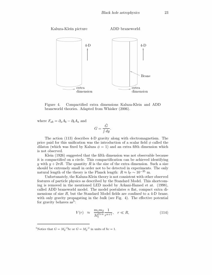
Figure 4. Compactified extra dimensions Kaluza-Klein and ADDbraneworld theories. Adapted from Whisker (2006).
where Fab = ∂aAb − ∂bAa and
G =G∫dy.
The action (113) describes 4-D gravity along with electromagnetism. Theprice paid for this unification was the introduction of a scalar field φ called thedilaton (which was fixed by Kaluza φ = 1) and an extra fifth dimension whichis not observed.
Klein (1926) suggested that the fifth dimension was not observable becauseit is compactified on a circle. This compactification can be achieved identifyingy with y + 2πR. The quantity R is the size of the extra dimension. Such a sizeshould be extremely small in order not to be detected in experiments. The onlynatural length of the theory is the Planck length: R ≈ lP ∼ 10−35 m.
Unfortunately, the Kaluza-Klein theory is not consistent with other observedfeatures of particle physics as described by the Standard Model. This shortcom-ing is removed in the mentioned LED model by Arkani-Hamed et at. (1998),called ADD braneworld model. The model postulates n flat, compact extra di-mensions of size R, but the Standard Model fields are confined to a 4-D brane,with only gravity propagating in the bulk (see Fig. 4). The effective potentialfor gravity behaves as5:
V (r) ≈ m1m2
M2+nf
1
rn+1, r � R, (114)
5Notice that G = M−2P hc or G = M−2
P in units of hc = 1.
24 Gustavo E. Romero
V (r) ≈ m1m2
M2+nf
1
Rnr, r � R, (115)
whereMf is the fundamental mass scale of gravity in the full (4+n)-D space-time.Hence, in the brane the effective 4-D Planck scale is given by:
M2P =M2+n
f Rn. (116)
In this way the fundamental scaleMf can be much lower than the Planck mass. Ifthe fundamental scale is comparable to the electroweak scale, Mfc
2 ∼Me−wc2 ∼
1 TeV, then we have that n ≥ 2.Randall and Sundrum (1999) suggested that the bulk geometry might be
curved and the brane could have a tension. Hence, the brane becomes a gravi-tating object, interacting dynamically with the bulk. A Randall-Sundrum (RS)universe consists of two branes of torsion σ1 and σ2 bounding a slice of an anti-de Sitter space6. The two branes are separated by a distance L and the fifthdimension y is periodic with period 2L. The bulk Einstein equations read:
Rab − 1
2Rgab = Λ5gab, (117)
where the bulk cosmological constant Λ5 can be expressed in terms of the cur-vature length l as:
Λ5 =6
l2. (118)
The metric is:ds2 = a2(y)ημνdx
μdxν + dy2. (119)
Using the previous expressions, we can write the metric as:
ds2 = e−2|y|/lημνdxμdxν + dy2. (120)
The term e−2|y|/l is called the warp factor. The effective Planck mass becomes:
M2P = e2L/lM3
f l. (121)
According to the ratio L/l, the effective Planck mass can change. If we wish tohave Mfc
2 ∼ 1 TeV, then we need L/l ∼ 50 in order to generate the observedPlanck mass Mfc
2 ∼ 1019 GeV.Other RS universes consist of a single, positive tension brane immersed in
an infinite (non-compact) extra dimension. The corresponding metric remainsthe same:
ds2 = e−2|y|/lημνdxμdxν + dy2.
The 5-D graviton propagates through the bulk, but only the zero (massless)mode moves on the brane (for details see Maartens 2004).
6An anti-de Sitter space-time has a metric that is a maximally symmetric vacuum solution ofEinstein’s field equations with an attractive cosmological constant (corresponding to a negativevacuum energy density and positive pressure). This space-time has a constant negative scalarcurvature.
Black hole astrophysics 25
10.3. f(R)-Gravity
In f(R) gravity, the Lagrangian of the Einstein-Hilbert action:
S[g] =
∫1
2κR√−g d4x (122)
is generalized to
S[g] =
∫1
2κf(R)
√−g d4x, (123)
where g is the determinant of the metric tensor g ≡ |gμν | and f(R) is somefunction of the scalar (Ricci) curvature.
The field equations are obtained by varying with respect to the metric. Thevariation of the determinant is:
δ√−g = −1
2
√−ggμνδgμν .
The Ricci scalar is defined as
R = gμνRμν .
Therefore, its variation with respect to the inverse metric gμν is given by
δR = Rμνδgμν + gμνδRμν
= Rμνδgμν + gμν(∇ρδΓ
ρνμ −∇νδΓ
ρρμ) (124)
Since δΓλμν is actually the difference of two connections, it should transform as
a tensor. Therefore, it can be written as
δΓλμν =
1
2gλa (∇μδgaν +∇νδgaμ −∇aδgμν) ,
and substituting in the equation above:
δR = Rμνδgμν + gμν�δg
μν −∇μ∇νδgμν .
The variation in the action reads:
δS[g] =1
2κ
∫ (δf(R)
√−g + f(R)δ√−g) d4x
=1
2κ
∫ (F (R)δR
√−g − 1
2
√−ggμνδgμνf(R))
d4x
=1
2κ
∫ √−g(F (R)(Rμνδg
μν + gμν�δgμν −∇μ∇νδg
μν)− 1
2gμνδg
μνf(R)
)d4x,
where F (R) = ∂f(R)∂R . Doing integration by parts on the second and third terms
we get:
δS[g] =1
2κ
∫ √−gδgμν(F (R)Rμν − 1
2gμνf(R) + [gμν�−∇μ∇ν ]F (R)
)d4x.
26 Gustavo E. Romero
By demanding that the action remains invariant under variations of themetric, i.e. δS[g] = 0, we obtain the field equations:
F (R)Rμν − 1
2f(R)gμν + [gμν�−∇μ∇ν ]F (R) = κTμν , (125)
where Tμν is the energy-momentum tensor defined as
Tμν = − 2√−gδ(√−gLm)
δgμν,
and Lm is the matter Lagrangian. If F (R) = 1, i.e. f(R) = R we recoverEinstein’s theory.
11. What is a star?
The idea that stars are self-gravitating gaseous bodies was introduced in th XIXCentury by Lane, Kelvin and Helmholtz. They suggested that stars should beunderstood in terms of the equation of hydrostatic equilibrium:
dP (r)
dr= −GM(r)ρ(r)
r2, (126)
where the pressure P is given by
P =ρkT
μmp. (127)
Here, k is Boltzmann’s constant, μ is the mean molecular weight, T the temper-ature, ρ the mass density, and mp the mass of the proton. Kelvin and Helmholtzsuggested that the source of heat was due to the gravitational contraction. How-ever, if the luminosity of a star like the Sun is taken into account, the totalenergy available would be released in 107 yr, which is in contradiction with thegeological evidence that can be found on Earth. Eddington made two fundamen-tal contributions to the theory of stellar structure proposing i) that the sourceof energy was thermonuclear reactions and ii) that the outward pressure of ra-diation should be included in Eq. (126). Then, the basic equations for stellarequilibrium become (Eddington 1926):
d
dr
[ρkT
μmp+
1
3aT 4
]= −GM(r)ρ(r)
r2, (128)
dPrad(r)
dr= −
(L(r)
4πr2c
)1
l, (129)
dL(r)
dr= 4πr2ερ, (130)
where l is the mean free path of the photons, L the luminosity, and ε the energygenerated per gram of material per unit time.
Black hole astrophysics 27
Once the nuclear power of the star is exhausted, the contribution from theradiation pressure decreases dramatically when the temperature diminishes. Thestar then contracts until a new pressure helps to balance gravity attraction: thedegeneracy pressure of the electrons. The equation of state for a degenerate gasof electrons is:
Prel = Kρ4/3. (131)
Then, using Eq. (126),
M4/3
r5∝ GM2
r5. (132)
Since the radius cancels out, this relations can be satisfied by a unique mass:
M = 0.197
[(hc
G
)3 1
m2p
]1
μ2e= 1.4 M�, (133)
where μe is the mean molecular weight of the electrons. The result implies thata completely degenerated star has this and only this mass. This limit was foundby Chandrasekhar (1931) and is known as the Chandrasekhar limit.
In 1939 Chandrasekhar conjectured that massive stars could develop a de-generate core. If the degenerate core attains sufficiently high densities the pro-tons and electrons will combine to form neutrons. “This would cause a suddendiminution of pressure resulting in the collapse of the star to the neutron coregiving rise to an enormous liberation of gravitational energy. This may be theorigin of the supernova phenomenon.” (Chandrasekhar 1939). An implicationof this prediction is that the masses of neutron stars (objects supported by thedegeneracy pressure of nucleons) should be close to 1.4 M�, the maximum massfor white dwarfs. Not long before, Baade and Zwicky commented: “With allreserve we advance the view that supernovae represent the transitions from or-dinary stars into neutron stars which in their final stages consist of extremelyclosely packed neutrons”. In this single paper Baade and Zwicky not only in-vented neutron stars and provided a theory for supernova explosions, but alsoproposed the origin of cosmic rays in these explosions (Baade & Zwicky 1934).
In the 1930s, neutron stars were not taken as a serious physical possibility.Oppenheimer & Volkoff (1939) concluded that if the neutron core was massiveenough, then “either the Fermi equation of state must fail at very high densi-ties, or the star will continue to contract indefinitely never reaching equilibrium”.In a subsequent paper Oppenheimer & Snyder (1939) chose between these twopossibilities: “when all thermonuclear sources of energy are exhausted a suffi-ciently heavy star will collapse. This contraction will continue indefinitely tillthe radius of the star approaches asymptotically its gravitational radius. Lightfrom the surface of the star will be progressively reddened and can escape over aprogressively narrower range of angles till eventually the star tends to close itselfoff from any communication with a distant observer”. What we now understandfor a black hole was then conceived. The scientific community paid no attentionto these results, and Oppenheimer and many other scientists turned their effortsto win a war.
28 Gustavo E. Romero
Black stars: an historical note
It is usual in textbooks to credit for the idea of black holes to John Michell andPierre-Simon Laplace, in the XVIII Century. The idea of a body so massive thateven light could not escape was put forward by geologist Rev. John Michell ina letter written to Henry Cavendish in 1783 to the Royal Society: “If the semi-diameter of a sphere of the same density as the Sun were to exceed that of theSun in the proportion of 500 to 1, a body falling from an infinite height towardit would have acquired at its surface greater velocity than that of light, andconsequently supposing light to be attracted by the same force in proportion toits inertia, with other bodies, all light emitted from such a body would be madeto return toward it by its own proper gravity.” (Michell 1783).
In 1796, the mathematician Pierre-Simon Laplace promoted the same ideain the first and second editions of his book Exposition du système du Monde(it was removed from later editions). Such “dark stars” were largely ignored inthe nineteenth century, since light was then thought to be a massless wave andtherefore not influenced by gravity. Unlike the modern black hole concept, theobject behind the horizon is assumed to be stable against collapse. Moreover, noequation of state was adopted neither by Michell nor Laplace. Hence, their darkstars where Newtonian objects, infinitely rigid, and they have nothing to do withthe nature of space and time, which were for the absolute concepts. Nonetheless,they could calculate correctly the size of such objects form the simple devise ofequating the potential and escape energy from a body of mass M :
1
2mv2 =
GMm
r2. (134)
Just setting v = c and assuming the gravitational and the inertial mass are thesame, we get:
rblack star =
√2GM
c2. (135)
12. Schwarzschild black holes
The first exact solution of Einstein field equations was found by Karl Schwarzschildin 1916. This solution describes the geometry of space-time outside a sphericallysymmetric matter distribution.
The most general spherically symmetric metric is:
ds2 = α(r, t)dt2 − β(r, t)dr2 − γ(r, t)dΩ2 − δ(r, t)drdt, (136)
where dΩ2 = dθ2 + sin2 θdφ2. We are using spherical polar coordinates. Themetric (136) is invariant under rotations (isotropic).
The invariance group of general relativity is formed by the group of generaltransformations of coordinates of the form x′μ = fμ(x). This yields 4 degreesof freedom, two of which have been used when adopting spherical coordinates(the transformations that do not break the central symmetry are: r′ = f1(r, t)and t′ = f2(r, t)). With the two available degrees of freedom we can freelychoose two metric coefficients, whereas the other two are determined by Einsteinequations. Some possibilities are:
Black hole astrophysics 29
• Standard gauge.
ds2 = c2A(r, t)dt2 −B(r, t)dr2 − r2dΩ2.
• Synchronous gauge.
ds2 = c2dt2 − F 2(r, t)dr2 −R2(r, t)dΩ2.
• Isotropic gauge.
ds2 = c2H2(r, t)dt2 −K2(r, t)[dr2 + r2(r, t)dΩ2
].
• Co-moving gauge.
ds2 = c2W 2(r, t)dt2 − U(r, t)dr2 − V (r, t)dΩ2.
Adopting the standard gauge and a static configuration (no dependence ofthe metric coefficients on t), we can get equations for the coefficients A and Bof the standard metric:
ds2 = c2A(r)dt2 −B(r)dr2 − r2dΩ2. (137)
Since we are interested in the solution outside the spherical mass distribution,we only need to require the Ricci tensor to vanish:
Rμν = 0.
According to the definition of the curvature tensor and the Ricci tensor, we have:
Rμν = ∂νΓσμσ − ∂σΓ
σμν + Γρ
μσΓσρν − Γρ
μνΓσρσ = 0. (138)
If we remember that the affine connection depends on the metric as
Γσμν =
1
2gρσ(∂νgρμ + ∂μgρν − ∂ρgμν),
we see that we have to solve a set of differential equations for the components ofthe metric gμν .
The metric coefficients are:
g00 = c2A(r),
g11 = −B(r),
g22 = −r2,g33 = −r2 sin2 θ,g00 = 1/A(r),
g11 = −1/B(r),
g22 = −1/r2,
g33 = −1/r2 sin2 θ.
30 Gustavo E. Romero
Then, only nine of the 40 independent connection coefficients are differentfrom zero. They are:
Γ101 = A′/(2A),
Γ122 = −r/B,
Γ233 = − sin θ cos θ,
Γ100 = A′/(2B),
Γ133 = −(r sin2 /B),
Γ313 = 1/r,
Γ111 = B′/(2B),
Γ212 = 1/r,
Γ323 = cot θ, .
Replacing in the expression for Rμν :
R00 = −A′′
2B+A′
4B
(A′
A+B′
B
)− A′
rB,
R11 =A′′
2A− A′
4A
(A′
A+B′
B
)− B′
rB,
R22 =1
B− 1 +
r
2B
(A′
A− B′
B
),
R33 = R22 sin2 θ.
The Einstein field equations for the region of empty space then become:
R00 = R11 = R22 = 0
(the fourth equation has no additional information). Multiplying the first equa-tion by B/A and adding the result to the second equation, we get:
A′B +AB′ = 0,
from which AB = constant. We can write then B = αA−1. Going to the thirdequation and replacing B we obtain: A+ rA′ = α, or:
d(rA)
dr= α.
The solution of this equation is:
A(r) = α
(1 +
k
r
),
with k another integration constant. For B we get:
B =
(1 +
k
r
)−1
.
Black hole astrophysics 31
If now we consider the Newtonian limit:
A(r)
c2= 1 +
2Φ
c2,
with Φ the Newtonian gravitational potential: Φ = −GM/r, we can concludethat
k = −2GM
c2
andα = c2.
Therefore, the Schwarzschild solution for a static mass M can be written inspherical coordinates (t, r, θ, φ) as:
ds2 =
(1− 2GM
rc2
)c2dt2 −
(1− 2GM
rc2
)−1
dr2 − r2(dθ2 + sin2 θdφ2). (139)
As mentioned, this solution corresponds to the vacuum region exterior to thespherical object of mass M . Inside the object, space-time will depend on thepeculiarities of the physical object.
The metric given by Eq. (139) has some interesting properties. Let’s assumethat the mass M is concentrated at r = 0. There seems to be two singularitiesat which the metric diverges: one at r = 0 and the other at
rSchw =2GM
c2. (140)
rSchw is know as the Schwarzschild radius. If the object of massM is macroscopic,then rSchw is inside it, and the solution does not apply. For instance, for the SunrSchw ∼ 3 km. However, for a point mass, the Schwarzschild radius is in thevacuum region and space-time has the structure given by (139). In general, wecan write:
rSchw ∼ 3
(M
M�
)km.
It is easy to see that strange things occur close to rSchw. For instance, forthe proper time we get:
dτ =
(1− 2GM
rc2
)1/2
dt, (141)
or
dt =
(1− 2GM
rc2
)−1/2
dτ, (142)
When r −→ ∞ both times agree, so t is interpreted as the proper timemeasure from an infinite distance. As the system with proper time τ approachesto rSchw, dt tends to infinity according to Eq. (142). The object never reachesthe Schwarszchild surface when seen by an infinitely distant observer. The closerthe object is to the Schwarzschild radius, the slower it moves for the externalobserver.

32 Gustavo E. Romero
A direct consequence of the difference introduced by gravity in the localtime respect to the time at infinity is that the radiation that escapes from agiven r > rSchw will be redshifted when received by a distant and static observer.Since the frequency (and hence the energy) of the photon depend of the timeinterval, we can write, from Eq. (142):
λ∞ =
(1− 2GM
rc2
)−1/2
λ. (143)
Since the redshift is:z =
λ∞ − λ
λ, (144)
then
1 + z =
(1− 2GM
rc2
)−1/2
, (145)
and we see that when r −→ rSchw the redshift becomes infinite. This meansthat a photon needs infinite energy to escape from inside the region determinedby rSchw. Events that occur at r < rSchw are disconnected from the rest of theuniverse. Hence, we call the surface determined by r = rSchw an event horizon.Whatever crosses the event horizon will never return. This is the origin of theexpression “black hole”, introduced by John A. Wheeler in the mid 1960s. Theblack hole is the region of space-time inside the event horizon. We can see whathappens with the light cones as an event is closer to the horizon of a Schwarzschildblack hole in Figure 5. The shape of the cones can be calculated from the metric(139) imposing the null condition ds2 = 0. Then,
dr
dt= ±
(1− 2GM
r
), (146)
where we made c = 1. Notice that when r → ∞, dr/dt → ±1, as in Minkowskispace-time. When r → 2GM , dr/dt → 0, and light moves along the surfacer = 2GM . For r < 2GM , the sign of the derivative is inverted. The inwardregion of r = 2GM is time-like for any physical system that has crossed theboundary surface.
What happens to an object when it crosses the event horizon?. Accordingto Eq. (139), there is a singularity at r = rSchw. However, the metric coefficientscan be made regular by a change of coordinates. For instance we can considerEddington-Finkelstein coordinates. Let us define a new radial coordinate r∗ suchthat radial null rays satisfy d(ct±r∗) = 0. Using Eq. (139) it can be shown that:
r∗ = r +2GM
c2log
∣∣∣∣∣r − 2GM/c2
2GM/c2
∣∣∣∣∣ .Then, we introduce:
v = ct+ r∗.
The new coordinate v can be used as a time coordinate replacing t in Eq. (139).This yields:
ds2 =
(1− 2GM
rc2
)(c2dt2 − dr2∗)− r2dΩ2
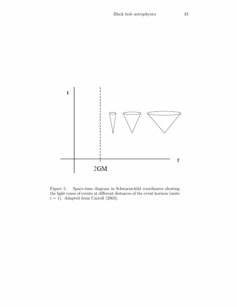
Black hole astrophysics 33
Figure 5. Space-time diagram in Schwarzschild coordinates showingthe light cones of events at different distances of the event horizon (unitsc = 1). Adapted form Carroll (2003).
34 Gustavo E. Romero
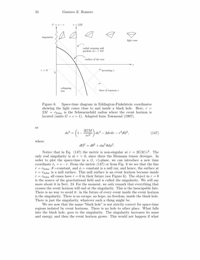
Figure 6. Space-time diagram in Eddington-Finkelstein coordinatesshowing the light cones close to and inside a black hole. Here, r =2M = rSchw is the Schwarzschild radius where the event horizon islocated (units G = c = 1). Adapted form Townsend (1997).
ords2 =
(1− 2GM
rc2
)dv2 − 2drdv − r2dΩ2, (147)
wheredΩ2 = dθ2 + sin2 θdφ2.
Notice that in Eq. (147) the metric is non-singular at r = 2GM/c2. Theonly real singularity is at r = 0, since there the Riemann tensor diverges. Inorder to plot the space-time in a (t, r)-plane, we can introduce a new timecoordinate t∗ = v− r. From the metric (147) or from Fig. 6 we see that the liner = rSchw, θ =constant, and φ = constant is a null ray, and hence, the surface atr = rSchw is a null surface. This null surface is an event horizon because insider = rSchw all cones have r = 0 in their future (see Figure 6). The object in r = 0is the source of the gravitational field and is called the singularity. We will saymore about it in Sect. 24. For the moment, we only remark that everything thatcrosses the event horizon will end at the singularity. This is the inescapable fate.There is no way to avoid it: in the future of every event inside the event horizonis the singularity. There is no escape, no hope, no freedom, inside the black hole.There is just the singularity, whatever such a thing might be.
We see now that the name “black hole” is not strictly correct for space-timeregions isolated by event horizons. There is no hole to other place. What fallsinto the black hole, goes to the singularity. The singularity increases its massand energy, and then the event horizon grows. This would not happen if what
Black hole astrophysics 35
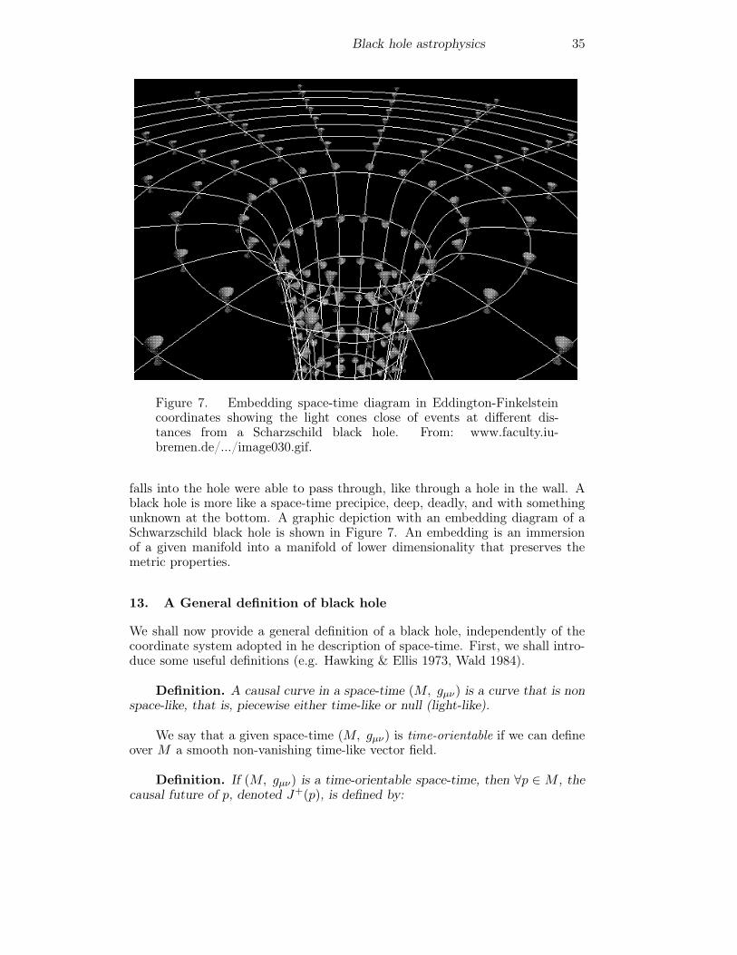
Figure 7. Embedding space-time diagram in Eddington-Finkelsteincoordinates showing the light cones close of events at different dis-tances from a Scharzschild black hole. From: www.faculty.iu-bremen.de/.../image030.gif.
falls into the hole were able to pass through, like through a hole in the wall. Ablack hole is more like a space-time precipice, deep, deadly, and with somethingunknown at the bottom. A graphic depiction with an embedding diagram of aSchwarzschild black hole is shown in Figure 7. An embedding is an immersionof a given manifold into a manifold of lower dimensionality that preserves themetric properties.
13. A General definition of black hole
We shall now provide a general definition of a black hole, independently of thecoordinate system adopted in he description of space-time. First, we shall intro-duce some useful definitions (e.g. Hawking & Ellis 1973, Wald 1984).
Definition. A causal curve in a space-time (M, gμν) is a curve that is nonspace-like, that is, piecewise either time-like or null (light-like).
We say that a given space-time (M, gμν) is time-orientable if we can defineover M a smooth non-vanishing time-like vector field.
Definition. If (M, gμν) is a time-orientable space-time, then ∀p ∈ M , thecausal future of p, denoted J+(p), is defined by:
36 Gustavo E. Romero
J+(p) ≡ {q ∈M |∃ a future− directed causal curve from p to q} . (148)
Similarly,
Definition. If (M, gμν) is a time-orientable space-time, then ∀p ∈ M , thecausal past of p, denoted J−(p), is defined by:
J−(p) ≡ {q ∈M |∃ a past− directed causal curve from p to q} . (149)
Particle horizons occur whenever a particular system never gets to be influ-enced by the whole space-time. If a particle crosses the horizon, it will not exertany further action upon the system respect to which the horizon is defined.
Definition. For a causal curve γ the associated future (past) particle hori-zon is defined as the boundary of the region from which the causal curves canreach some point on γ.
Finding the particle horizons (if one exists at all) requires a knowledge ofthe global space-time geometry.
Let us now consider a space-time where all null geodesics that start in aregion J − end at J +. Then, such a space-time, (M, gμν) is said to contain ablack hole if M is not contained in J−(J +). In other words, there is a regionfrom where no null geodesic can reach the asymptotic flat7 future space-time, or,equivalently, there is a region of M that is causally disconnected from the globalfuture. The black hole region, BH, of such space-time is BH = [M − J−(J +)],and the boundary of BH in M , H = J−(J +)
⋂M , is the event horizon.
14. Birkoff’s theorem
If we consider the isotropic but not static line element,
ds2 = c2A(r, t)dt2 −B(r, t)dr2 − r2dΩ2, (150)
and substitute into the Einstein empty-space field equations Rμν = 0 to obtainthe functions A(r, t) and B(r, t), the result would be exactly the same:
A(r, t) = A(r) =
(1− 2GM
rc2
),
and
B(r, t) = B(r) =
(1− 2GM
rc2
)−1
.
7Asymptotic flatness is the property of a geometry of space-time which means that in appropriatecoordinates, the limit of the metric at infinity approaches the metric of the flat (Minkowskian)space-time.
Black hole astrophysics 37
This result is general and known as the Birkoff’s theorem:
The space-time geometry outside a general spherical symmetry matter dis-tribution is the Schwarzschild geometry.
Birkoff’s theorem implies that strictly radial motions do not perturb thespace-time metric. In particular, a pulsating star, if the pulsations are strictlyradial, does not produce gravitational waves.
The converse of Birkoff’s theorem is not true, i.e.,
If the region of space-time is described by the metric given by expression(139), then the matter distribution that is the source of the metric does not needto be spherically symmetric.
15. Orbits
Orbits around a Schwarzschild black hole can be easily calculated using themetric and the relevant symmetries (see. e.g. Raine and Thomas 2005). Letus call kμ a vector in the direction of a given symmetry (i.e. kμ is a Killingvector). A static situation is symmetric in the time direction, hence we canwrite: kμ = (1, 0, 0, 0). The 4-velocity of a particle with trajectory xμ = xμ(τ)is uμ = dxμ/dτ . Then, since u0 = E/c, where E is the energy, we have:
gμνkμuν = g00k
0u0 = g00u0 = η00
E
c=E
c= constant. (151)
If the particle moves along a geodesic in a Schwarzschild space-time, we obtainfrom Eq. (151):
c
(1− 2GM
c2r
)dt
dτ=E
c. (152)
Similarly, for the symmetry in the azimuthal angle φ we have kμ = (0, 0, 0, 1),in such a way that:
gμνkμuν = g33k
3u3 = g33u3 = −L = constant. (153)
In the Schwarzschild metric we find, then,
r2dφ
dτ= L = constant. (154)
If now we divide the Schwarzschild interval (139) by c2dτ2:
1 =
(1− 2GM
c2r
)(dt
dτ
)2
− c−2(1− 2GM
c2r
)−1 (drdτ
)2
− c−2r2(dφ
dτ
)2
, (155)
and using the conservation equations (152) and (154) we obtain:(dr
dτ
)2
=E2
c2−(c2 +
L2
r2
)(1− 2GM
c2r
). (156)
38 Gustavo E. Romero
If we express energy in units of m0c2 and introduce an effective potential Veff ,(
dr
dτ
)2
=E2
c2− V 2
eff . (157)
For circular orbits of a massive particle we have the conditions
dr
dτ= 0, and
d2r
dτ2= 0.
The orbits are possible only at the turning points of the effective potential:
Veff =
√(c2 +
L2
r2
)(1− 2rg
r
), (158)
where L is the angular momentum in units of m0c and rg = GM/c2 is thegravitational radius. Then,
r =L2
2crg± 1
2
√L4
c2r2g− 12L2. (159)
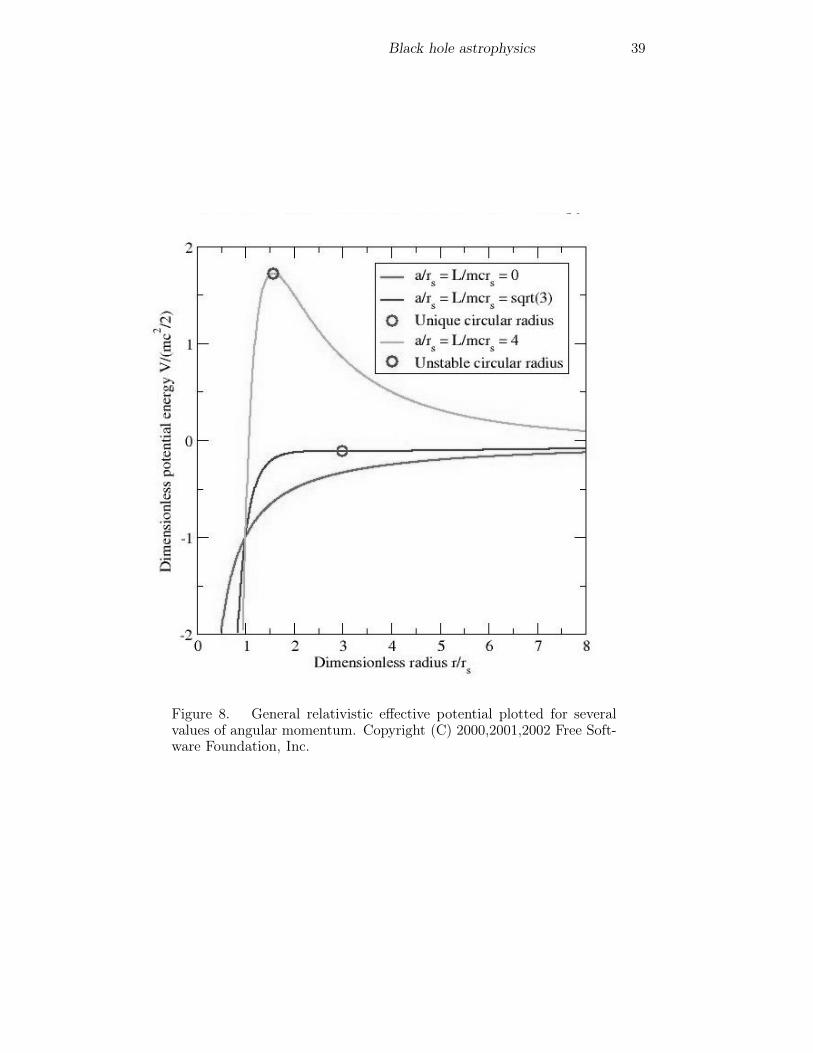
The effective potential is shown in Figure 8 for different values of the angularmomentum.
For L2 > 12c2r2g there are two solutions. The negative sign corresponds toa maximum of the potential and is unstable, and the positive sign correspondsto a minimum, which is stable. At L2 = 12c2r2g there is a single stable orbit. Itis the innermost marginally stable orbit, and it occurs at r = 6rg = 3rSchw. Thespecific angular momentum of a particle in a circular orbit at r is:
L = c
(rgr
1− 3rg/r
)1/2
.
Its energy (units of m0c2) is:
E =
(1− 2rg
r
)(1− 3rg
r
)−1/2
.
The proper and observer’s periods are:
τ =2π
c
(r3
rg
)1/2 (1− 3rg
r
)1/2
and
T =2π
c
(r3
rg
)1/2
.
Notice that when r −→ 3rg both L and E tend to infinity, so only masslessparticles can orbit at such a radius.
Black hole astrophysics 39
Figure 8. General relativistic effective potential plotted for severalvalues of angular momentum. Copyright (C) 2000,2001,2002 Free Soft-ware Foundation, Inc.
40 Gustavo E. Romero
The local velocity at r of an object falling from rest to the black hole is (e.g.Raine and Thomas 2005):
vloc =proper distance
proper time=
dr
(1− 2GM/c2r) dt,
hence, using the expression for dr/dt from the metric (139):
dr
dt= −c
(2GM
c2r
)1/2 (1− 2GM
c2r
), (160)
we have,
vloc =
(2rgr
)1/2
(in units of c). (161)
Then, the differential acceleration the object will experience along an element dris8:
dg =2rgr3c2 dr. (162)
The tidal acceleration on a body of finite size Δr is simply (2rg/r3)c2 Δr. This
acceleration and the corresponding force becomes infinite at the singularity. Asthe object falls into the black hole, tidal forces act to tear it apart. This painfulprocess is known as “spaghettification”. The process can be significant long beforecrossing the event horizon, depending on the mass of the black hole.
The energy of a particle in the innermost stable orbit can be obtained fromthe above equation for the energy setting r = 6rg. This yields (unites of m0c
2):
E =
(1− 2rg
6rg
)(1− 3rg
6rg
)−1/2
=2
3
√2.
Since a particle at rest at infinity has E = 1, then the energy that the particleshould release to fall into the black hole is 1− (2/3)
√2 = 0.057. This means 5.7
% of its rest mass energy, significantly higher than the energy release that canbe achieved through nuclear fusion.
An interesting question we can ask is what is the gravitational accelerationat the event horizon as seen by an observer from infinity. The acceleration relativeto a hovering frame system of a freely falling object at rest at r is (Raine andThomas 2005):
gr = −c2(GM/c2
r2
)(1− 2GM/c2
r
)−1/2
.
So, the energy spent to move the object a distance dl will be dEr = mgrdl. Theenergy expended respect to a frame at infinity is dE∞ = mg∞dl. Because of theconservation of energy, both quantities should be related by a redshift factor:
Er
E∞=
grg∞
=
(1− 2GM/c2
r
)−1/2
.
8Notice that dvloc/dτ = (dvloc/dr)(dr/dτ ) = (dvloc/dr)vloc = rgc2/r2.
Black hole astrophysics 41
Hence, using the expression for gr we get:
g∞ = c2GM/c2
r2. (163)
Notice that for an observer at r, gr −→ ∞ when r −→ rSchw. However, frominfinity the required force to hold the object hovering at the horizon is:
mg∞ = c2GmM/c2
r2Schw=
mc4
4GM.
This is the surface gravity of the black hole.
Radial motion of photons
For photons we have that ds2 = 0. The radial motion, then, satisfies:(1− 2GM
rc2
)c2dt2 −
(1− 2GM
rc2
)−1
dr2 = 0. (164)
From here,dr
dt= ±c
(1− 2GM
rc2
). (165)
Integrating, we have:
ct = r +2GM
c2ln
∣∣∣∣∣ rc22GM− 1
∣∣∣∣∣ + constant outgoing photons, (166)
ct = −r − 2GM
c2ln
∣∣∣∣∣ rc22GM− 1
∣∣∣∣∣+ constant incoming photons. (167)
Notice that in a (ct, r)-diagram the photons have worldlines with slopes±1 as r → ∞, indicating that space-time is asymptotically flat. As the eventsthat generate the photons approach to r = rSchw, the slopes tend to ±∞. Thismeans that the light cones become more and more thin for events close to theevent horizon. At r = rSchw the photons cannot escape and they move along thehorizon (see Fig. 5). An observer in the infinity will never detect them.
Circular motion of photons
In this case, fixing θ =constant due to the symmetry, we have that photons willmove in a circle of r =constant and ds2 = 0. Then, from (139), we have:(
1− 2GM
rc2
)c2dt2 − r2dφ2 = 0. (168)
This means that
φ =c
r
√(1− 2GM
rc2
)= constant.
42 Gustavo E. Romero
The circular velocity is:
vcirc =rφ√g00
=Ωr
(1− 2GM/c2r)1/2. (169)
Setting vcirc = c for photons and using Ω = (GM/r3)1/2, we get that the onlypossible radius for a circular photon orbit is:
rph =3GM
c2. (170)
For a compact object of 1 M�, r ≈ 4.5 km, in comparison with the Schwarzschildradius of 3 km. Photons moving at this distance form the “photosphere” of theblack hole. The orbit, however, is unstable, as it can be seen from the effectivepotential:
Veff =L2ph
r2
(1− 2rg
r
). (171)
Notice that the four-acceleration for circular motion is: aμ = uμuν ;ν . The
radial component in the Schawrzschild metric is:
ar =GM/r2 − Ω2r
1− 2GM/c2r − Ω2r2/c2. (172)
The circular motion along a geodesic line corresponds to the case ar = 0 (freemotion). This gives from Eq. (172) the usual expression for the Keplerianangular velocity
ΩK =
(GM
r3
)1/2
,
already used in deriving rph. In general, however, the angular velocity can haveany value determined by the metric and can be quite different from the corre-sponding Keplerian value. In general:
v =rΩK
(1− 2GM/c2r)1/2=
(GM
r
)1/2 (1− 2GM
c2r
)−1/2
. (173)
From this latter equation and the fact that v ≤ c it can be concluded that pureKeplerian motion is only possible for r ≥ 1.5rSchw. At r ≤ 1.5rSchw any massiveparticle will find its mass increased by special relativistic effects in such a waythat the gravitational attraction will outweigh any centrifugal force.
Gravitational capture
A particle coming from infinity is captured if its trajectory ends in the black hole.The angular momentum of a non-relativistic particle with velocity v∞ at infinityis L = mv∞b, where b is an impact parameter. The condition L/mcrSchw = 2defines bcr, non−rel = 2rSchw(c/v∞). Then, the capture cross section is:
σnon−rel = πb2cr = 4πc2r2Schwv2∞
. (174)
Black hole astrophysics 43
For an ultra-relativistic particle, bcr = 3√3rSchw/2, and then
σrel = πb2cr =27
4πr2Schw. (175)
16. Other coordinate systems
Other coordinates can be introduced to study additional properties of black holes.We refer the reader to the books of Frolov and Novikov (1998) and Raine andThomas (2005) for further details. Here we shall only introduce the Kruskal-Szekeres coordinates. These coordinates have the advantage that they cover theentire space-time manifold of the maximally extended Schwarzschild solutionand are well-behaved everywhere outside the physical singularity. They allow toremove the non-physical singularity at r = rSchw and provide new insights onthe interior solution, on which we will return later.
Let us consider the following coordinate transformation:
u =
(r
rSchw− 1
)1/2
er
2rSchw cosh
(ct
2rSchw
),
v =
(r
rSchw− 1
)1/2
er
2rSchw sinh
(ct
2rSchw
), (176)
if r > rSchw,
and
u =
(1− r
rSchw
)1/2
er
2rSchw sinh
(ct
2rSchw
),
v =
(1− r
rSchw
)1/2
er
2rSchw cosh
(ct
2rSchw
), (177)
if r < rSchw.
The line element in the Kruskal-Szekeres coordinates is completely regular,except at r = 0:
ds2 =4r3Schwr
er
rSchw
(dv2 − du2
)− r2dΩ2. (178)
The curves at r = constant are hyperbolic and satisfy:
u2 − v2 =
(r
rSchw− 1
)1/2
er
rSchw , (179)
whereas the curves at t = constant are straight lines that pass through the origin:u
v= tanh
ct
2rSchw, r < rSchw,
u
v= coth
ct
2rSchw, r > rSchw. (180)
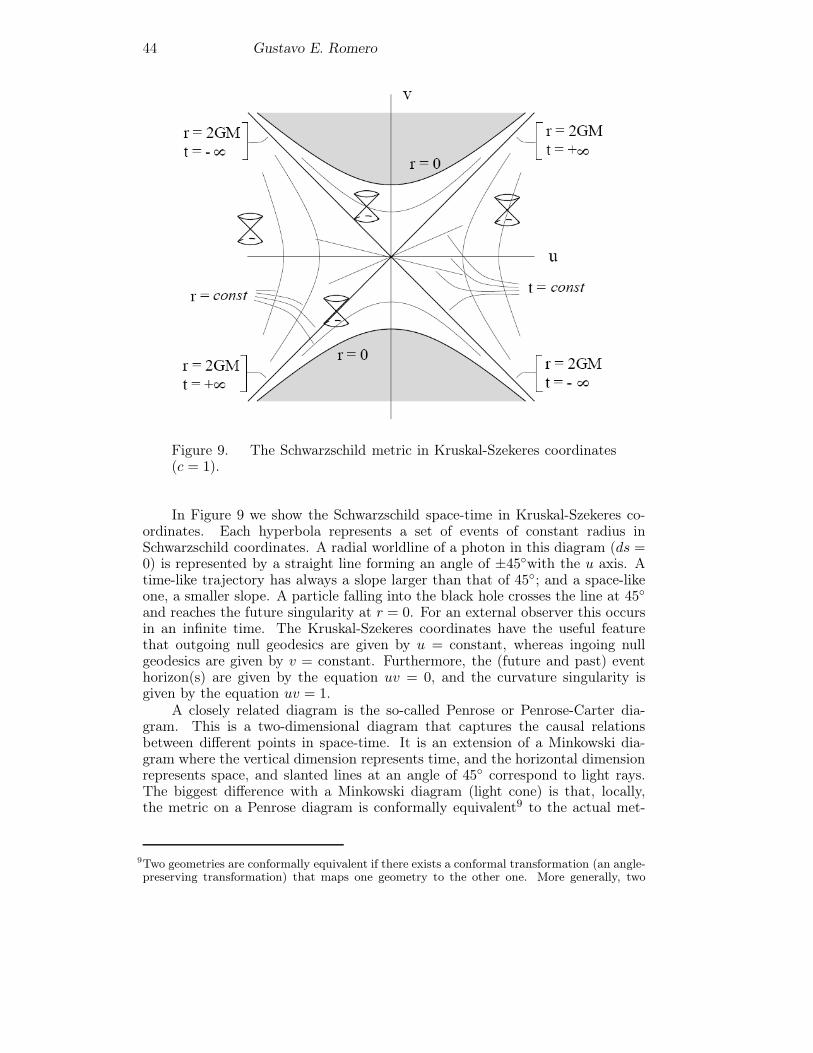
44 Gustavo E. Romero
Figure 9. The Schwarzschild metric in Kruskal-Szekeres coordinates(c = 1).
In Figure 9 we show the Schwarzschild space-time in Kruskal-Szekeres co-ordinates. Each hyperbola represents a set of events of constant radius inSchwarzschild coordinates. A radial worldline of a photon in this diagram (ds =0) is represented by a straight line forming an angle of ±45◦with the u axis. Atime-like trajectory has always a slope larger than that of 45◦; and a space-likeone, a smaller slope. A particle falling into the black hole crosses the line at 45◦and reaches the future singularity at r = 0. For an external observer this occursin an infinite time. The Kruskal-Szekeres coordinates have the useful featurethat outgoing null geodesics are given by u = constant, whereas ingoing nullgeodesics are given by v = constant. Furthermore, the (future and past) eventhorizon(s) are given by the equation uv = 0, and the curvature singularity isgiven by the equation uv = 1.
A closely related diagram is the so-called Penrose or Penrose-Carter dia-gram. This is a two-dimensional diagram that captures the causal relationsbetween different points in space-time. It is an extension of a Minkowski dia-gram where the vertical dimension represents time, and the horizontal dimensionrepresents space, and slanted lines at an angle of 45◦ correspond to light rays.The biggest difference with a Minkowski diagram (light cone) is that, locally,the metric on a Penrose diagram is conformally equivalent9 to the actual met-
9Two geometries are conformally equivalent if there exists a conformal transformation (an angle-preserving transformation) that maps one geometry to the other one. More generally, two
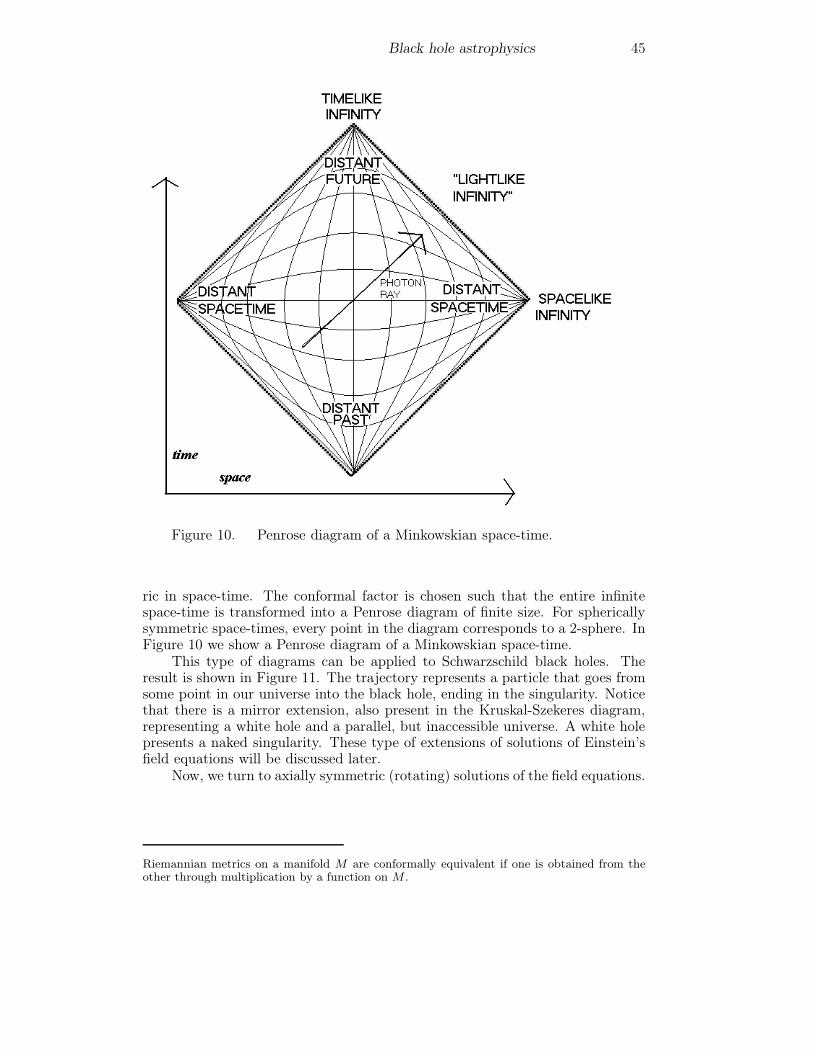
Black hole astrophysics 45
Figure 10. Penrose diagram of a Minkowskian space-time.
ric in space-time. The conformal factor is chosen such that the entire infinitespace-time is transformed into a Penrose diagram of finite size. For sphericallysymmetric space-times, every point in the diagram corresponds to a 2-sphere. InFigure 10 we show a Penrose diagram of a Minkowskian space-time.
This type of diagrams can be applied to Schwarzschild black holes. Theresult is shown in Figure 11. The trajectory represents a particle that goes fromsome point in our universe into the black hole, ending in the singularity. Noticethat there is a mirror extension, also present in the Kruskal-Szekeres diagram,representing a white hole and a parallel, but inaccessible universe. A white holepresents a naked singularity. These type of extensions of solutions of Einstein’sfield equations will be discussed later.
Now, we turn to axially symmetric (rotating) solutions of the field equations.
Riemannian metrics on a manifold M are conformally equivalent if one is obtained from theother through multiplication by a function on M .
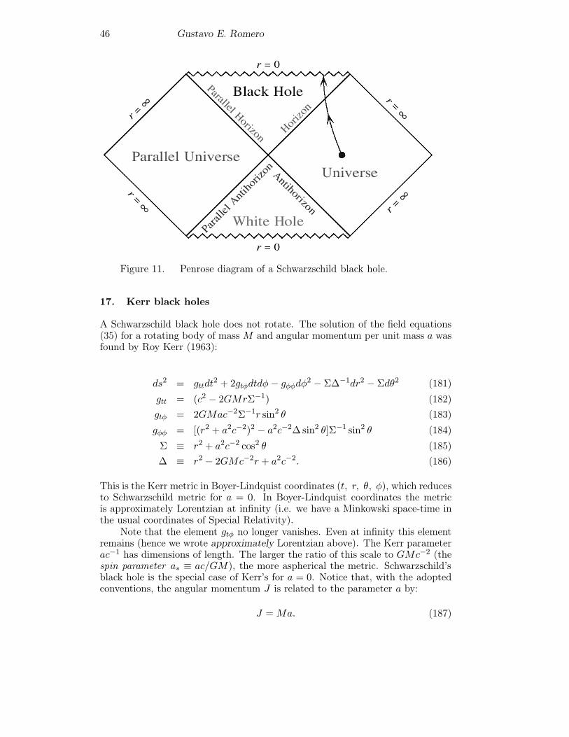
46 Gustavo E. Romero
Figure 11. Penrose diagram of a Schwarzschild black hole.
17. Kerr black holes
A Schwarzschild black hole does not rotate. The solution of the field equations(35) for a rotating body of mass M and angular momentum per unit mass a wasfound by Roy Kerr (1963):
ds2 = gttdt2 + 2gtφdtdφ− gφφdφ
2 − ΣΔ−1dr2 − Σdθ2 (181)gtt = (c2 − 2GMrΣ−1) (182)gtφ = 2GMac−2Σ−1r sin2 θ (183)gφφ = [(r2 + a2c−2)2 − a2c−2Δsin2 θ]Σ−1 sin2 θ (184)Σ ≡ r2 + a2c−2 cos2 θ (185)Δ ≡ r2 − 2GMc−2r + a2c−2. (186)
This is the Kerr metric in Boyer-Lindquist coordinates (t, r, θ, φ), which reducesto Schwarzschild metric for a = 0. In Boyer-Lindquist coordinates the metricis approximately Lorentzian at infinity (i.e. we have a Minkowski space-time inthe usual coordinates of Special Relativity).
Note that the element gtφ no longer vanishes. Even at infinity this elementremains (hence we wrote approximately Lorentzian above). The Kerr parameterac−1 has dimensions of length. The larger the ratio of this scale to GMc−2 (thespin parameter a∗ ≡ ac/GM), the more aspherical the metric. Schwarzschild’sblack hole is the special case of Kerr’s for a = 0. Notice that, with the adoptedconventions, the angular momentum J is related to the parameter a by:
J =Ma. (187)
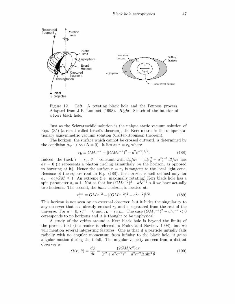
Black hole astrophysics 47
Figure 12. Left: A rotating black hole and the Penrose process.Adapted from J-P. Luminet (1998). Right: Sketch of the interior ofa Kerr black hole.
Just as the Schwarzschild solution is the unique static vacuum solution ofEqs. (35) (a result called Israel’s theorem), the Kerr metric is the unique sta-tionary axisymmetric vacuum solution (Carter-Robinson theorem).
The horizon, the surface which cannot be crossed outward, is determined bythe condition grr → ∞ (Δ = 0). It lies at r = rh where
rh ≡ GMc−2 + [(GMc−2)2 − a2c−2]1/2. (188)
Indeed, the track r = rh, θ = constant with dφ/dτ = a(r2h + a2)−1 dt/dτ hasdτ = 0 (it represents a photon circling azimuthaly on the horizon, as opposedto hovering at it). Hence the surface r = rh is tangent to the local light cone.Because of the square root in Eq. (188), the horizon is well defined only fora∗ = ac/GM ≤ 1. An extreme (i.e. maximally rotating) Kerr black hole has aspin parameter a∗ = 1. Notice that for (GMc−2)2 − a2c−2 > 0 we have actuallytwo horizons. The second, the inner horizon, is located at:
rinnh ≡ GMc−2 − [(GMc−2)2 − a2c−2]1/2. (189)
This horizon is not seen by an external observer, but it hides the singularity toany observer that has already crossed rh and is separated from the rest of theuniverse. For a = 0, rinnh = 0 and rh = rSchw. The case (GMc−2)2 − a2c−2 < 0corresponds to no horizons and it is thought to be unphysical.
A study of the orbits around a Kerr black hole is beyond the limits ofthe present text (the reader is referred to Frolov and Novikov 1998), but wewill mention several interesting features. One is that if a particle initially fallsradially with no angular momentum from infinity to the black hole, it gainsangular motion during the infall. The angular velocity as seen from a distantobserver is:
Ω(r, θ) =dφ
dt=
(2GM/c2)ar
(r2 + a2c−2)2 − a2c−2Δsin2 θ. (190)
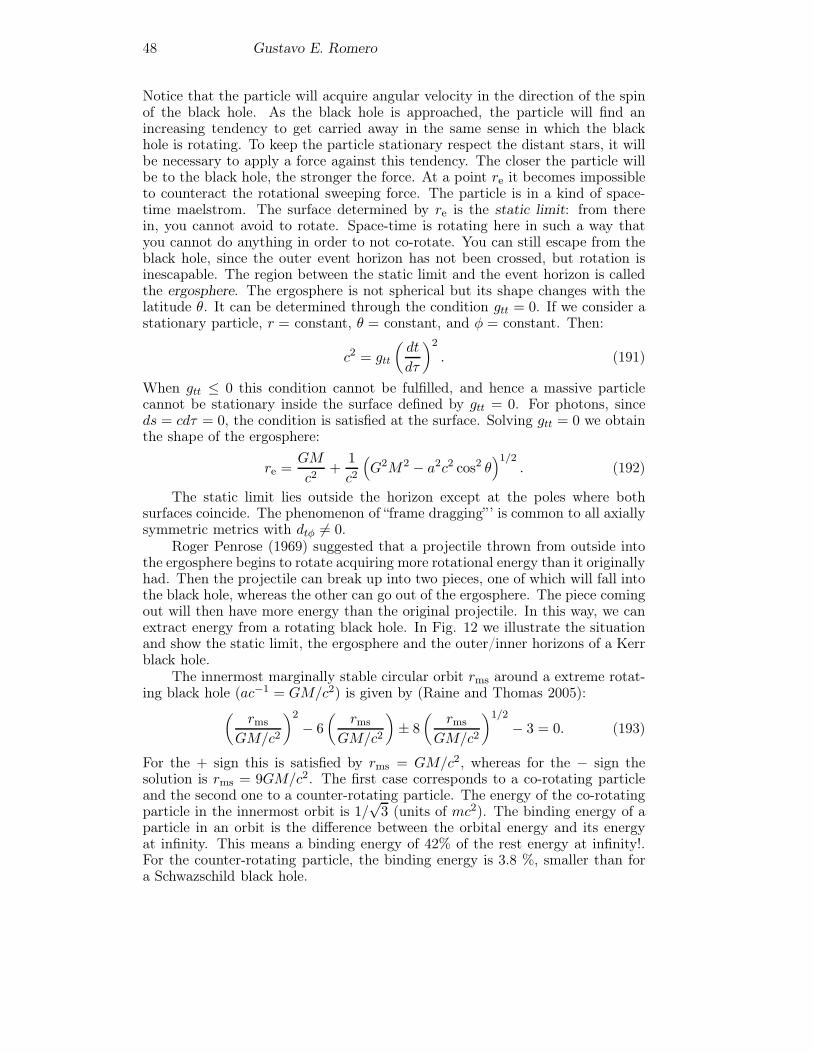
48 Gustavo E. Romero
Notice that the particle will acquire angular velocity in the direction of the spinof the black hole. As the black hole is approached, the particle will find anincreasing tendency to get carried away in the same sense in which the blackhole is rotating. To keep the particle stationary respect the distant stars, it willbe necessary to apply a force against this tendency. The closer the particle willbe to the black hole, the stronger the force. At a point re it becomes impossibleto counteract the rotational sweeping force. The particle is in a kind of space-time maelstrom. The surface determined by re is the static limit: from therein, you cannot avoid to rotate. Space-time is rotating here in such a way thatyou cannot do anything in order to not co-rotate. You can still escape from theblack hole, since the outer event horizon has not been crossed, but rotation isinescapable. The region between the static limit and the event horizon is calledthe ergosphere. The ergosphere is not spherical but its shape changes with thelatitude θ. It can be determined through the condition gtt = 0. If we consider astationary particle, r = constant, θ = constant, and φ = constant. Then:
c2 = gtt
(dt
dτ
)2
. (191)
When gtt ≤ 0 this condition cannot be fulfilled, and hence a massive particlecannot be stationary inside the surface defined by gtt = 0. For photons, sinceds = cdτ = 0, the condition is satisfied at the surface. Solving gtt = 0 we obtainthe shape of the ergosphere:
re =GM
c2+
1
c2
(G2M2 − a2c2 cos2 θ
)1/2. (192)
The static limit lies outside the horizon except at the poles where bothsurfaces coincide. The phenomenon of “frame dragging” ’ is common to all axiallysymmetric metrics with dtφ �= 0.
Roger Penrose (1969) suggested that a projectile thrown from outside intothe ergosphere begins to rotate acquiring more rotational energy than it originallyhad. Then the projectile can break up into two pieces, one of which will fall intothe black hole, whereas the other can go out of the ergosphere. The piece comingout will then have more energy than the original projectile. In this way, we canextract energy from a rotating black hole. In Fig. 12 we illustrate the situationand show the static limit, the ergosphere and the outer/inner horizons of a Kerrblack hole.
The innermost marginally stable circular orbit rms around a extreme rotat-ing black hole (ac−1 = GM/c2) is given by (Raine and Thomas 2005):(
rms
GM/c2
)2
− 6
(rms
GM/c2
)± 8
(rms
GM/c2
)1/2
− 3 = 0. (193)
For the + sign this is satisfied by rms = GM/c2, whereas for the − sign thesolution is rms = 9GM/c2. The first case corresponds to a co-rotating particleand the second one to a counter-rotating particle. The energy of the co-rotatingparticle in the innermost orbit is 1/
√3 (units of mc2). The binding energy of a
particle in an orbit is the difference between the orbital energy and its energyat infinity. This means a binding energy of 42% of the rest energy at infinity!.For the counter-rotating particle, the binding energy is 3.8 %, smaller than fora Schwazschild black hole.
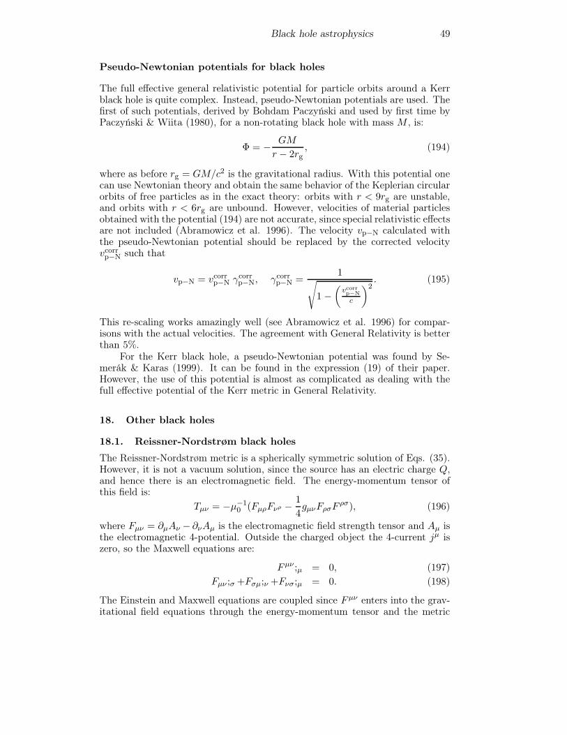
Black hole astrophysics 49
Pseudo-Newtonian potentials for black holes
The full effective general relativistic potential for particle orbits around a Kerrblack hole is quite complex. Instead, pseudo-Newtonian potentials are used. Thefirst of such potentials, derived by Bohdam Paczyński and used by first time byPaczyński & Wiita (1980), for a non-rotating black hole with mass M , is:
Φ = − GM
r − 2rg, (194)
where as before rg = GM/c2 is the gravitational radius. With this potential onecan use Newtonian theory and obtain the same behavior of the Keplerian circularorbits of free particles as in the exact theory: orbits with r < 9rg are unstable,and orbits with r < 6rg are unbound. However, velocities of material particlesobtained with the potential (194) are not accurate, since special relativistic effectsare not included (Abramowicz et al. 1996). The velocity vp−N calculated withthe pseudo-Newtonian potential should be replaced by the corrected velocityvcorrp−N such that
vp−N = vcorrp−N γcorrp−N, γcorrp−N =
1√1−
(vcorrp−N
c
)2. (195)
This re-scaling works amazingly well (see Abramowicz et al. 1996) for compar-isons with the actual velocities. The agreement with General Relativity is betterthan 5%.
For the Kerr black hole, a pseudo-Newtonian potential was found by Se-merák & Karas (1999). It can be found in the expression (19) of their paper.However, the use of this potential is almost as complicated as dealing with thefull effective potential of the Kerr metric in General Relativity.
18. Other black holes
18.1. Reissner-Nordstrøm black holes
The Reissner-Nordstrøm metric is a spherically symmetric solution of Eqs. (35).However, it is not a vacuum solution, since the source has an electric charge Q,and hence there is an electromagnetic field. The energy-momentum tensor ofthis field is:
Tμν = −μ−10 (FμρFνρ − 1
4gμνFρσF
ρσ), (196)
where Fμν = ∂μAν − ∂νAμ is the electromagnetic field strength tensor and Aμ isthe electromagnetic 4-potential. Outside the charged object the 4-current jμ iszero, so the Maxwell equations are:
Fμν ;μ = 0, (197)Fμν ;σ +Fσμ;ν +Fνσ;μ = 0. (198)
The Einstein and Maxwell equations are coupled since Fμν enters into the grav-itational field equations through the energy-momentum tensor and the metric

50 Gustavo E. Romero
gμν enters into the electromagnetic equations through the covariant derivative.Because of the symmetry constraints we can write:
[Aμ] =
(ϕ(r)
c2, a(r), 0, 0
), (199)
where ϕ(r) is the electrostatic potential, and a(r) is the radial component of the3-vector potential as r −→ ∞.
The solution for the metric is given by
ds2 = Δc2dt2 −Δ−1dr2 − r2dΩ2 , (200)
where
Δ = 1− 2GM/c2
r+q2
r2. (201)
In this expression, M is once again interpreted as the mass of the hole and
q =GQ2
4πε0c4(202)
is related to the total electric charge Q.The metric has a coordinate singularity at Δ = 0, in such a way that:
r± = rg ± (r2g − q2)1/2. (203)
Here, rg = GM/c2 is the gravitational radius. For rg = q, we have an extremeReissner-Nordstrøm black hole with a unique horizon at r = rg. Notice that aReissner-Nordstrøm black hole can be more compact than a Scharzschild blackhole of the same mass. For the case r2g > q2, both r± are real and there aretwo horizons as in the Kerr solution. Finally, in the case r2g < q2 both r±are imaginary there is no coordinate singularities, no horizon hides the intrinsicsingularity at r = 0. It is thought, however, that naked singularities do not existin nature (see Section 24. below).
18.2. Kerr-Newman black holes
The Kerr-Newman metric of a charged spinning black hole is the most generalblack hole solution. It was found by Ezra “Ted” Newman in 1965 (Newman etal. 1965). This metric can be obtained from the Kerr metric (181) in Boyer-Lindquist coordinates by the replacement:
2GM
c2r −→ 2GM
c2r − a2c−2 − q2,
where q is related to the charge Q by Eq. (202).The full expression reads:
ds2 = gttdt2 + 2gtφdtdφ− gφφdφ
2 − ΣΔ−1dr2 − Σdθ2 (204)gtt = (c2 − 2GMrΣ−2) (205)gtφ = 2GMac−2Σ−1r sin2 θ (206)gφφ = [(r2 + a2c−2)2 − a2c−2Δsin2 θ]Σ−1 sin2 θ (207)Σ ≡ r2 + a2c−2 cos2 θ (208)Δ ≡ r2 − 2GMc−2r + a2c−2 + q2 ≡ (r − routh )(r − rinnh ), (209)
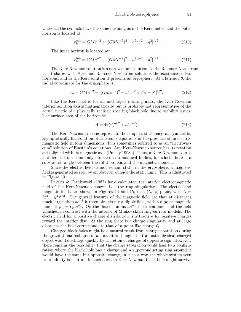
Black hole astrophysics 51
where all the symbols have the same meaning as in the Kerr metric and the outerhorizon is located at:
routh = GMc−2 + [(GMc−2)2 − a2c−2 − q2]1/2. (210)
The inner horizon is located at:
rinnh = GMc−2 − [(GMc−2)2 − a2c−2 − q2]1/2. (211)
The Kerr-Newman solution is a non-vacuum solution, as the Reissner-Nordstrømis. It shares with Kerr and Reissner-Nordstrøm solutions the existence of twohorizons, and as the Kerr solution it presents an ergosphere. At a latitude θ, theradial coordinate for the ergosphere is:
re = GMc−2 − [(GMc−2)2 − a2c−2 sin2 θ − q2]1/2. (212)
Like the Kerr metric for an uncharged rotating mass, the Kerr-Newmaninterior solution exists mathematically but is probably not representative of theactual metric of a physically realistic rotating black hole due to stability issues.The surface area of the horizon is:
A = 4π(rout 2h + a2c−2). (213)
The Kerr-Newman metric represents the simplest stationary, axisymmetric,asymptotically flat solution of Einstein’s equations in the presence of an electro-magnetic field in four dimensions. It is sometimes referred to as an “electrovac-cum” solution of Einstein’s equations. Any Kerr-Newman source has its rotationaxis aligned with its magnetic axis (Punsly 1998a). Thus, a Kerr-Newman sourceis different from commonly observed astronomical bodies, for which there is asubstantial angle between the rotation axis and the magnetic moment.
Since the electric field cannot remain static in the ergosphere, a magneticfield is generated as seen by an observer outside the static limit. This is illustratedin Figure 13.
Pekeris & Frankowski (1987) have calculated the interior electromagneticfield of the Kerr-Newman source, i.e., the ring singularity. The electric andmagnetic fields are shown in Figures 14 and 15, in a (λ, z)-plane, with λ =
(x2 + y2)1/2. The general features of the magnetic field are that at distancesmuch larger than ac−1 it resembles closely a dipole field, with a dipolar magneticmoment μd = Qac−1. On the disc of radius ac−1 the z-component of the fieldvanishes, in contrast with the interior of Minkowskian ring-current models. Theelectric field for a positive charge distribution is attractive for positive chargestoward the interior disc. At the ring there is a charge singularity and at largedistances the field corresponds to that of a point like charge Q.
Charged black holes might be a natural result from charge separation duringthe gravitational collapse of a star. It is thought that an astrophysical chargedobject would discharge quickly by accretion of charges of opposite sign. However,there remains the possibility that the charge separation could lead to a configu-ration where the black hole has a charge and a superconducting ring around itwould have the same but opposite charge, in such a way the whole system seenfrom infinity is neutral. In such a case a Kerr-Newman black hole might survive
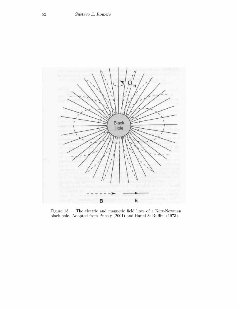
52 Gustavo E. Romero
Figure 13. The electric and magnetic field lines of a Kerr-Newmanblack hole. Adapted from Punsly (2001) and Hanni & Ruffini (1973).
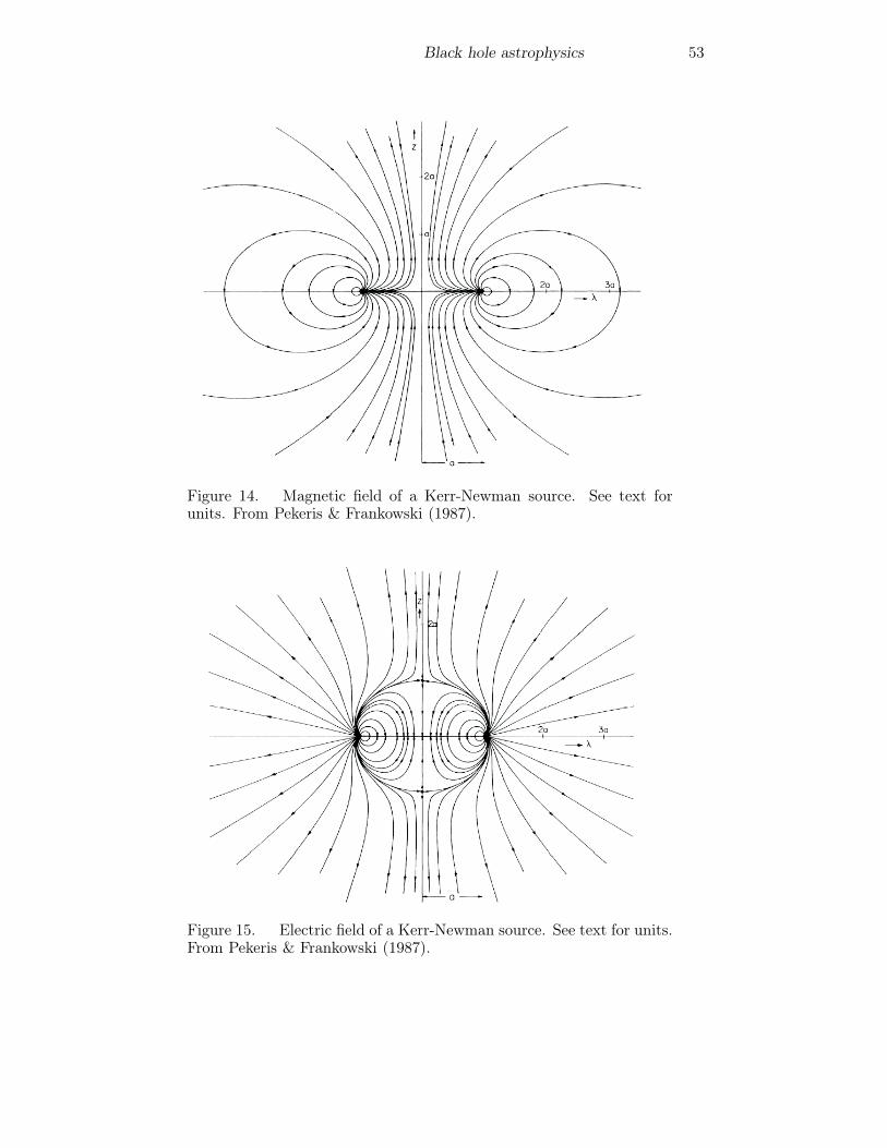
Black hole astrophysics 53
Figure 14. Magnetic field of a Kerr-Newman source. See text forunits. From Pekeris & Frankowski (1987).
Figure 15. Electric field of a Kerr-Newman source. See text for units.From Pekeris & Frankowski (1987).
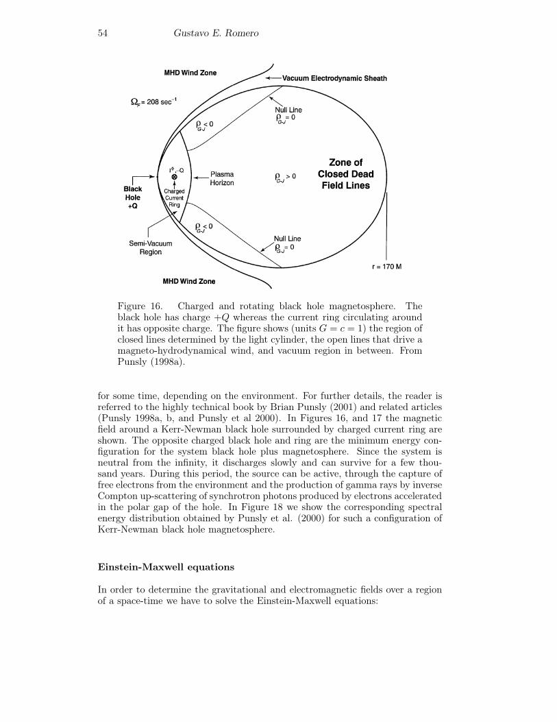
54 Gustavo E. Romero
Figure 16. Charged and rotating black hole magnetosphere. Theblack hole has charge +Q whereas the current ring circulating aroundit has opposite charge. The figure shows (units G = c = 1) the region ofclosed lines determined by the light cylinder, the open lines that drive amagneto-hydrodynamical wind, and vacuum region in between. FromPunsly (1998a).
for some time, depending on the environment. For further details, the reader isreferred to the highly technical book by Brian Punsly (2001) and related articles(Punsly 1998a, b, and Punsly et al 2000). In Figures 16, and 17 the magneticfield around a Kerr-Newman black hole surrounded by charged current ring areshown. The opposite charged black hole and ring are the minimum energy con-figuration for the system black hole plus magnetosphere. Since the system isneutral from the infinity, it discharges slowly and can survive for a few thou-sand years. During this period, the source can be active, through the capture offree electrons from the environment and the production of gamma rays by inverseCompton up-scattering of synchrotron photons produced by electrons acceleratedin the polar gap of the hole. In Figure 18 we show the corresponding spectralenergy distribution obtained by Punsly et al. (2000) for such a configuration ofKerr-Newman black hole magnetosphere.
Einstein-Maxwell equations
In order to determine the gravitational and electromagnetic fields over a regionof a space-time we have to solve the Einstein-Maxwell equations:
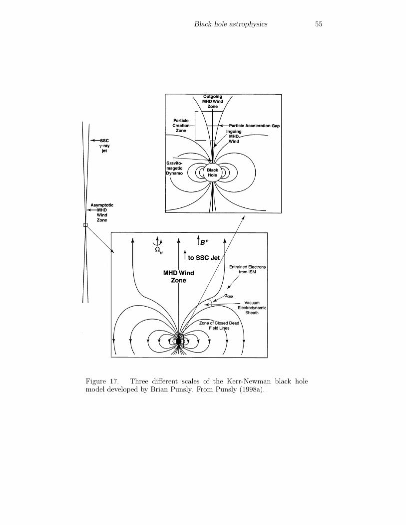
Black hole astrophysics 55
Figure 17. Three different scales of the Kerr-Newman black holemodel developed by Brian Punsly. From Punsly (1998a).
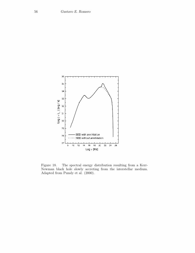
56 Gustavo E. Romero
� �� �� �� �� �� �� �� �� ��
��
��
��
�
�
�
�
�
��� ���� �������
��� ����� � �������
���
�ν�
��
���
��� ν ����
Figure 18. The spectral energy distribution resulting from a Kerr-Newman black hole slowly accreting from the interstellar medium.Adapted from Punsly et al. (2000).
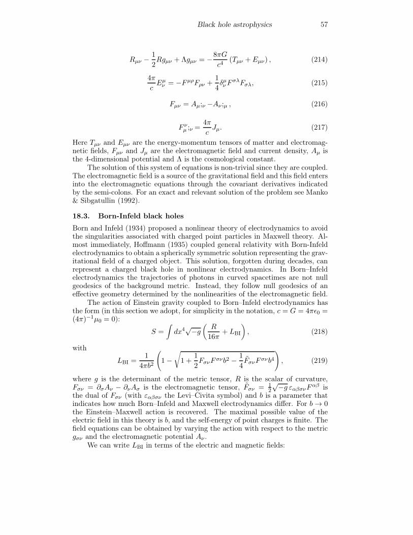
Black hole astrophysics 57
Rμν − 1
2Rgμν + Λgμν = −8πG
c4(Tμν +Eμν) , (214)
4π
cEμ
ν = −FμρFρν +1
4δμνF
σλFσλ, (215)
Fμν = Aμ;ν −Aν ;μ , (216)
F νμ ;ν =
4π
cJμ. (217)
Here Tμν and Eμν are the energy-momentum tensors of matter and electromag-netic fields, Fμν and Jμ are the electromagnetic field and current density, Aμ isthe 4-dimensional potential and Λ is the cosmological constant.
The solution of this system of equations is non-trivial since they are coupled.The electromagnetic field is a source of the gravitational field and this field entersinto the electromagnetic equations through the covariant derivatives indicatedby the semi-colons. For an exact and relevant solution of the problem see Manko& Sibgatullin (1992).
18.3. Born-Infeld black holes
Born and Infeld (1934) proposed a nonlinear theory of electrodynamics to avoidthe singularities associated with charged point particles in Maxwell theory. Al-most immediately, Hoffmann (1935) coupled general relativity with Born-Infeldelectrodynamics to obtain a spherically symmetric solution representing the grav-itational field of a charged object. This solution, forgotten during decades, canrepresent a charged black hole in nonlinear electrodynamics. In Born–Infeldelectrodynamics the trajectories of photons in curved spacetimes are not nullgeodesics of the background metric. Instead, they follow null geodesics of aneffective geometry determined by the nonlinearities of the electromagnetic field.
The action of Einstein gravity coupled to Born–Infeld electrodynamics hasthe form (in this section we adopt, for simplicity in the notation, c = G = 4πε0 =(4π)−1μ0 = 0):
S =
∫dx4
√−g(R
16π+ LBI
), (218)
with
LBI =1
4πb2
(1−
√1 +
1
2FσνF σνb2 − 1
4FσνF σνb4
), (219)
where g is the determinant of the metric tensor, R is the scalar of curvature,Fσν = ∂σAν − ∂νAσ is the electromagnetic tensor, Fσν = 1
2
√−g εαβσνFαβ isthe dual of Fσν (with εαβσν the Levi–Civita symbol) and b is a parameter thatindicates how much Born–Infeld and Maxwell electrodynamics differ. For b→ 0the Einstein–Maxwell action is recovered. The maximal possible value of theelectric field in this theory is b, and the self-energy of point charges is finite. Thefield equations can be obtained by varying the action with respect to the metricgσν and the electromagnetic potential Aν .
We can write LBI in terms of the electric and magnetic fields:
58 Gustavo E. Romero
LBI =b2
4π
⎡⎣1−√1− B2 − E2
b2− ( �E �B)2
b4
⎤⎦ . (220)
The Larangian depends non-linearly of the electromagnetic invariants:
F =1
4FαβF
αβ =1
2(B2 − E2), (221)
G =1
4FαβF
αβ = −B · E. (222)
Introducing the Hamiltonian formalism:
Pαβ = 2∂L
∂Fαβ=∂L
∂FFαβ +
∂L
∂GFαβ , (223)
H =1
2PαβFαβ − L(F, G2), (224)
and adopting the notation
P =1
4PαβP
αβ , (225)
Q =1
4PαβP
αβ , (226)
we can express Fαβ as a function of Pαβ, P , and Q:
Fαβ = 2∂H
∂Pαβ=∂H
∂PPαβ +
∂H
∂QPαβ. (227)
The Hamiltonian equations in the P and Q formalism can be written as:(∂H∂P
Pαβ +∂H
∂QPαβ
),β
= 0. (228)
.The couple Einstein-Born-Infeld equations are:
4πTμν =∂H
∂PPμαP
αν − gμν
(2P
∂H
∂P+ Q
∂H
∂Q−H
), (229)
R = 8
(P∂H
∂P+ Q
∂H
∂Q−H
). (230)
The field equations have spherically symmetric black hole solutions given by
ds2 = ψ(r)dt2 − ψ(r)−1dr2 − r2dΩ2, (231)
withψ(r) = 1− 2M
r+
2
b2r
∫ ∞
r
(√x4 + b2Q2 − x2
)dx, (232)

Black hole astrophysics 59
D(r) =QE
r2, (233)
B(r) = QM sin θ, (234)
where M is the mass, Q2 = Q2E + Q2
M is the sum of the squares of the electricQE and magnetic QM charges, B(r) and D(r) are the magnetic and the electricinductions in the local orthonormal frame. In the limit b → 0, the Reissner–Nordström metric is obtained. The metric (231) is also asymptotically Reissner–Norsdtröm for large values of r. With the units adopted above, M , Q and b havedimensions of length. The metric function ψ(r) can be expressed in the form
ψ(r) = 1−2M
r+
2
3b2
{r2 −
√r4 + b2Q2 +
√|bQ|3r
F
[arccos
(r2 − |bQ|r2 + |bQ|
),
√2
2
]},
(235)where F (γ, k) is the elliptic integral of the first kind10. As in Schwarzschild andReissner–Norsdtröm cases, the metric (231) has a singularity at r = 0 .
The zeros of ψ(r) determine the position of the horizons, which have to beobtained numerically. For a given value of b, when the charge is small, 0 ≤|Q|/M ≤ ν1, the function ψ(r) has one zero and there is a regular event horizon.For intermediate values of charge, ν1 < |Q|/M < ν2, ψ(r) has two zeros, sothere are, as in the Reissner–Nordström geometry, an inner horizon and an outerregular event horizon. When |Q|/M = ν2, there is one degenerate horizon.Finally, if the values of charge are large, |Q|/M > ν2, the function ψ(r) has nozeros and a naked singularity is obtained. The values of |Q|/M where the numberof horizons change, ν1 = (9|b|/M)1/3[F (π,
√2/2)]−2/3 and ν2, which should be
calculated numerically from the condition ψ(rh) = ψ′(rh) = 0, are increasingfunctions of |b|/M . In the Reissner–Nordström limit (b → 0) it is easy to seethat ν1 = 0 and ν2 = 1.
The paths of photons in nonlinear electrodynamics are not null geodesicsof the background geometry. Instead, they follow null geodesics of an effectivemetric generated by the self-interaction of the electromagnetic field, which de-pends on the particular nonlinear theory considered. In Einstein gravity coupledto Born–Infeld electrodynamics the effective geometry for photons is given by :
ds2eff = ω(r)1/2ψ(r)dt2 − ω(r)1/2ψ(r)−1dr2 − ω(r)−1/2r2dΩ2, (236)
where
ω(r) = 1 +Q2b2
r4. (237)
Then, to calculate the deflection angle for photons passing near the black holes,it is necessary to use the effective metric (236) instead of the background metric(231). The horizon structure of the effective metric is the same that of metric(231), but the trajectories of photons are different.
10F (γ, k) =∫ γ
0(1− k2 sin2 φ)−1/2dφ =
∫ sin γ
0[(1− z2)(1− k2z2)]−1/2dz
60 Gustavo E. Romero
18.4. Regular black holes
Solutions of Einstein’s field equations representing black holes where the metricis always regular (i.e. free of intrinsic singularities with RμνρσRμνρσ diverges)can be found for some choices of the equation of state. For instance, Mbonyeand Kazanas (2005) have sugested the following equation:
pr(ρ) =
[α− (α+ 1)
(ρ
ρmax
)m]( ρ
ρmax
)1/n
ρ. (238)
The maximum limiting density ρmax is concentrated in a region of radius:
r0 =
√1
Gρmax. (239)
At low densities pr ∝ ρ1+1/n and the equation reduces to that of a polytropegas. At high densities, close to ρmax the equation becomes pr = −ρ and thesystem behaves as a gravitational field dominated by a cosmological term in thefield equations. The exact values of m, n, and α determine the sound speed inthe system. Imposing that the maximum sound speed cs = (dp/dρ)1/2 be finiteeverywhere, is possible to constrain the free parameters. Adopting m = 2 andn = 1 the Eq. (238) becomes:
pr(ρ) =
[α− (α+ 1)
(ρ
ρmax
)2](
ρ
ρmax
)ρ. (240)
Then, the Schwarzschild solution can be written as:
ds2 =
(1− 2GM(r)
rc2
)eΓ(r)c2dt2 −
(1− 2GM(r)
rc2
)−1
dr2 − r2(dθ2 + sin2 θdφ2),
(241)where M(r) is the mass enclosed by a 2-sphere of radius r and:
Γ(r) =
∫8π
[α− (α+ 1)
(ρ
ρmax
)2](
ρ
ρmax
)(r
r − 2GM(r)
)ρdr. (242)
The mass within r isM(r) = 4π
∫ r
0ρ(r′)r′2dr′, (243)
and the total mass is
M =
∫ ∞
0M(r)dr =
∫ ∞
0ρ(r)r2dr. (244)
Since outside the body ρ → 0, Γ(r) → 1 and Eq. (241) becomes Schwarzschildsolution for Rμν = 0.
When r → 0, ρ = ρmax and the metric becomes of de Sitter type:
ds2 =
(1− r2
r20
)c2dt2 −
(1− r2
r20
)−1
dr2 − r2(dθ2 + sin2 θdφ2), (245)
Black hole astrophysics 61
with
r0 =
√3
8πGρmax. (246)
There is no singularity at r = 0 and the black hole is regular. For 0 ≤ r < 1 hasconstant positive density ρmax and negative pressure pr = −ρmax and space-timebecomes asymptotically de Sitter in the inner most region. It might be speculatedthat the transition in the equation of state occurs because at very high densitiesthe matter field couples with a scalar field that provides the negative pressure.
Other assumptions for the equation of state can lead to different (but stillregular) behavior, like a bouncing colse to r = 0 and the development of anexpanding closed universe inside the black hole (Frolov, Markov, and Mukhanov1990). In addition, regular black holes can be found in f(R) gravity for somesuitable function of the curvature scalar.
19. Black hole formation
Black holes will form every time that matter and fields are compressed beyondthe corresponding Schwarzschild radius. This can occur in a variety of forms,from particle collisions to the implosion of stars or the collapse of dark matterin the early universe. The most common black hole formation mechanism in ourGalaxy seems to be gravitational collapse. A normal star is stable as long as thenuclear reactions occurring in its interior provide thermal pressure to support itagainst gravity. Nuclear burning gradually transforms the stellar core from Hto He and in the case of massive stars (M > 5 M�) then to C and finally toFe. The core contracts in the processes, in order to achieve the ignition of eachphase of thermonuclear burning.
Finally, the endothermic disintegration of iron-group nuclei, which are thosewith the tightest bound, precipitates the collapse of the core to a stellar-massblack hole. Stars with masses in the range 20− 30M� produce black holes withM > 1.8 M�. Low-mass black holes (1.5 M� < M < 1.8 M�) can result fromthe collapse of stars of 18 − 20 M� along with the ejection of the outer layersof the star by a shock wave in an event known as Type II supernova. A similarevent, occurring in stars with 10 − 18 M� leaves behind a neutron star. Verymassive stars with high spin likely end producing a gamma-ray burst and a verymassive (M > 10 M�) black hole. The binary stellar systems have a differentevolution. The interested reader can find an comprehensive review in Brown etal. (2000).
In Figure 19 we show the Eddignton-Finkelstein diagram of the gravitationalcollapse of a star. Once the null surface of the light cones points along the timeaxis the black hole is formed: light rays will never be again able to escape to theouter universe. The different paths that can lead to a stellar mass black hole areillustrated in Figure 20.
If the collapse is not perfectly symmetric, any asymmetry in the resultingblack hole is radiated away as gravitational waves, in such a way that the finalresult is a black hole that is completely characterized by the three parametersM , J , and Q. The black hole, once formed, has no hints about the details of theformation process and its previous history.
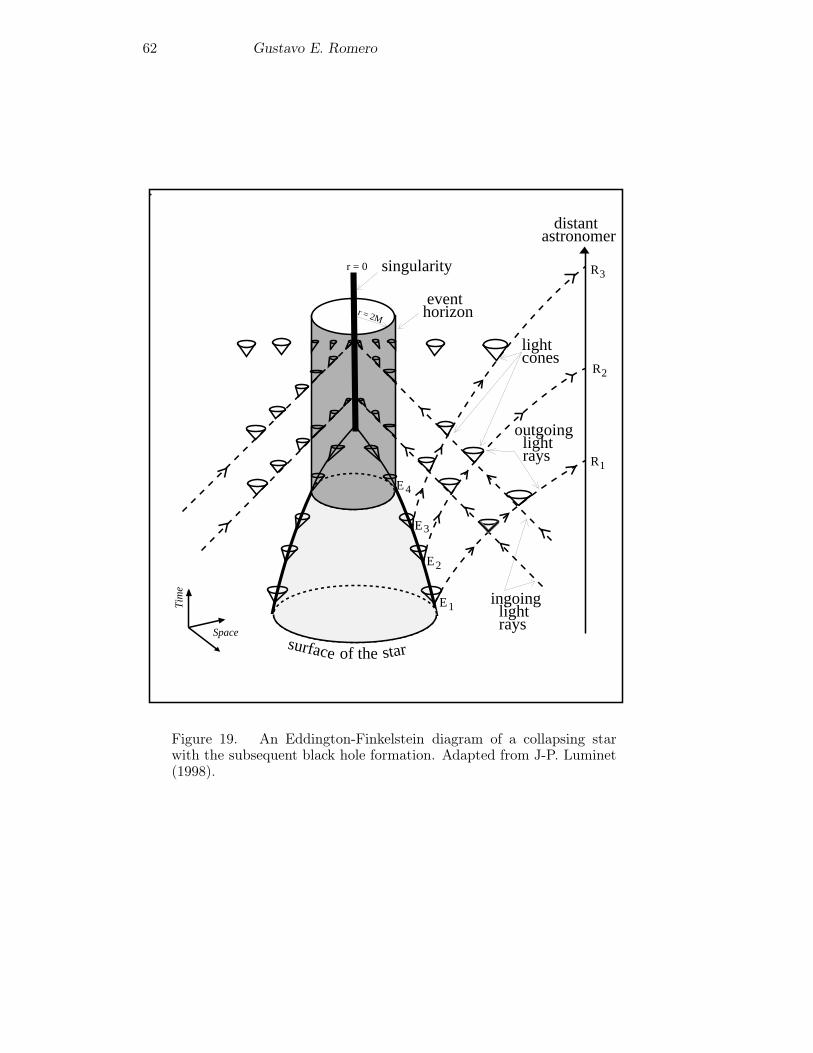
62 Gustavo E. Romero
R
R
R
E
E
E
E
1
1
2
2
3
3
4
r = 2M
r = 0 singularity
eventhorizon
distantastronomer
lightcones
ingoing light rays
outgoing light rays
surface of the star
Figure 4
Tim
e
Space
Figure 19. An Eddington-Finkelstein diagram of a collapsing starwith the subsequent black hole formation. Adapted from J-P. Luminet(1998).
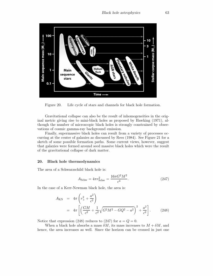
Black hole astrophysics 63
Figure 20. Life cycle of stars and channels for black hole formation.
Gravitational collapse can also be the result of inhomogeneities in the orig-inal metric giving rise to mini-black holes as proposed by Hawking (1971), al-though the number of microscopic black holes is strongly constrained by obser-vations of cosmic gamma-ray background emission.
Finally, supermassive black holes can result from a variety of processes oc-curring at the center of galaxies as discussed by Rees (1984). See Figure 21 for asketch of some possible formation paths. Some current views, however, suggestthat galaxies were formed around seed massive black holes which were the resultof the gravitational collapse of dark matter.
20. Black hole thermodynamics
The area of a Schwarzschild black hole is:
ASchw = 4πr2Schw =16πG2M2
c4. (247)
In the case of a Kerr-Newman black hole, the area is:
AKN = 4π
(r2+ +
a2
c2
)
= 4π
[(GM
c2+
1
c2
√G2M2 −GQ2 − a2
)2
+a2
c2
]. (248)
Notice that expression (248) reduces to (247) for a = Q = 0.When a black hole absorbs a mass δM , its mass increases to M + δM , and
hence, the area increases as well. Since the horizon can be crossed in just one
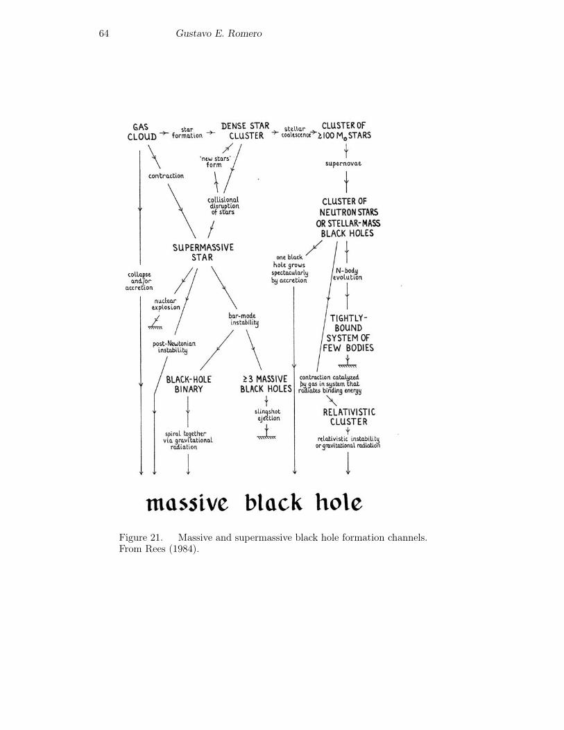
64 Gustavo E. Romero
Figure 21. Massive and supermassive black hole formation channels.From Rees (1984).
Black hole astrophysics 65
direction the area of a black hole can only increase. This suggests an analogywith entropy. A variation in the entropy of the black hole will be related to theheat (δQ) absorbed through the following equation:
δS =δQ
TBH=δMc2
TBH. (249)
Particles trapped in the black hole will have a wavelength:
λ =hc
kT∝ rSchw, (250)
where k is the Boltzmann constant. Then,
ξhc
kT=
2GM
c2,
where ξ is a numerical constant. Then,
TBH = ξhc3
2GkM, and S =
c6
32πG2M
∫dASchw
TBH=
c3k
16πhGξASchw + constant.
A quantum mechanical calculation of the horizon temperature in the Schwarzschildcase leads to ξ = (4π)−1 and hence:
TBH =hc3
8GMk∼= 10−7K
(M�M
). (251)
We can write then the entropy of the black hole as:
S =kc3
4πhGASchw + constant ∼ 1077
(M
M�
)2
k JK−1. (252)
The formation of a black hole implies a huge increase of entropy. Just to com-pare, a solar mass star has an entropy ∼ 20 orders of magnitude lower. Thistremendous increase of entropy is related to the loss of all the structure of theoriginal system (e.g. a star) once the black hole is formed.
The analogy between area and entropy allows to state a set of laws for blackholes thermodynamics:
• First law (energy conservation): dM = TBHdS +Ω+dJ +ΦdQ. Here, Ω isthe angular velocity and Φ the electrostatic potential.
• Second law (entropy never decreases): In all physical processes involvingblack holes the total surface area of all the participating black holes cannever decrease.
• Third law (Nernst’s law): The temperature (surface gravity) of a blackblack hole cannot be zero. Since TBH = 0 with A �= 0 for extremal chargedand extremal Kerr black holes, these are thought to be limit cases thatcannot be reached in Nature.
• Zeroth law (thermal equilibrium): The surface gravity (temperature) isconstant over the event horizon of a stationary axially symmetric blackhole.
66 Gustavo E. Romero
21. Quantum effects in black holes
If a temperature can be associated with black holes, then they should radiate asany other body. The luminosity of a Schwarzschild black hole is:
LBH = 4πr2SchwσT4BH ∼ 16πσh4c6
(8π)4G2M2k4. (253)
Here, σ is the Stephan-Boltzmann constant. This expression can be written as:
LBH = 10−17(M�M
)2
erg s−1. (254)
The lifetime of a black hole is:
τ ∼= M
dM/dt∼ 2.5 × 1063
(M
M�
)3
years. (255)
Notice that the black hole heats up as it radiates!. This occurs because when thehole radiates, its mass decreases and then according to Eq. (251) the temperaturemust rise.
If nothing can escape from black holes because of the existence of the eventhorizon, what is the origin of this radiation?. The answer, found by Hawking(1974), is related to quantum effects close to the horizon. According to theHeisenberg relation ΔtΔE ≥ h/2 particles can be created out of the groundstate of a quantum field as far as the relation is not violated. Particles must becreated in pairs, along a tiny time, in order to satisfy conservation laws otherthan energy. If a pair is created close to the horizon an one particle crossesit, then the other particle can escape provided its momentum is in the outwarddirection. The virtual particle is then transformed into a real particle, at expenseof the black hole energy. The black hole then will lose energy and its area willdecrease slowly, violating the second law of thermodynamics. However, there isno violation if we consider a generalized second law, that always holds: In anyprocess, the total generalized entropy S+SBH never decreases (Bekenstein 1973).
22. Black hole magnetospheres
In the real universe black holes are not expected to be isolated, hence the er-gosphere should be populated by charged particles. This plasma would rotatein the same sense as the black hole due to the effects of the frame dragging.A magnetic field will develop and will rotate too, generating a potential dropthat might accelerate particles up to relativistic speed and produce a wind alongthe rotation axis of the hole. Such a picture has been consistently developed byPunsly and Coroniti (1990a, b) and Punsly (2001).
In Figures 22 and 23 we show the behavior of fields and currents in theergosphere. Since the whole region is rotating, an ergospheric wind arises alongthe direction of the large scale field.
Blandford and Znajek (1977) developed a general theory of force-free steady-state axisymmetric magnetosphere of a rotating black hole. In an accreting black
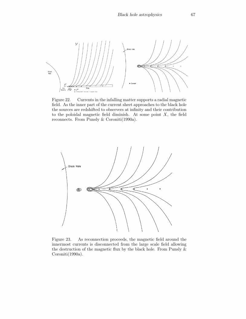
Black hole astrophysics 67
Figure 22. Currents in the infalling matter supports a radial magneticfield. As the inner part of the current sheet approaches to the black holethe sources are redshifted to observers at infinity and their contributionto the poloidal magnetic field diminish. At some point X, the fieldreconnects. From Punsly & Coroniti(1990a).
Figure 23. As reconnection proceeds, the magnetic field around theinnermost currents is disconnected from the large scale field allowingthe destruction of the magnetic flux by the black hole. From Punsly &Coroniti(1990a).
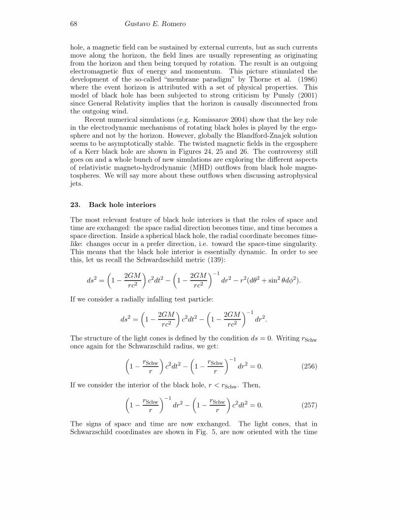
68 Gustavo E. Romero
hole, a magnetic field can be sustained by external currents, but as such currentsmove along the horizon, the field lines are usually representing as originatingfrom the horizon and then being torqued by rotation. The result is an outgoingelectromagnetic flux of energy and momentum. This picture stimulated thedevelopment of the so-called “membrane paradigm” by Thorne et al. (1986)where the event horizon is attributed with a set of physical properties. Thismodel of black hole has been subjected to strong criticism by Punsly (2001)since General Relativity implies that the horizon is causally disconnected fromthe outgoing wind.
Recent numerical simulations (e.g. Komissarov 2004) show that the key rolein the electrodynamic mechanisms of rotating black holes is played by the ergo-sphere and not by the horizon. However, globally the Blandford-Znajek solutionseems to be asymptotically stable. The twisted magnetic fields in the ergosphereof a Kerr black hole are shown in Figures 24, 25 and 26. The controversy stillgoes on and a whole bunch of new simulations are exploring the different aspectsof relativistic magneto-hydrodynamic (MHD) outflows from black hole magne-tospheres. We will say more about these outflows when discussing astrophysicaljets.
23. Back hole interiors
The most relevant feature of black hole interiors is that the roles of space andtime are exchanged: the space radial direction becomes time, and time becomes aspace direction. Inside a spherical black hole, the radial coordinate becomes time-like: changes occur in a prefer direction, i.e. toward the space-time singularity.This means that the black hole interior is essentially dynamic. In order to seethis, let us recall the Schwardzschild metric (139):
ds2 =
(1− 2GM
rc2
)c2dt2 −
(1− 2GM
rc2
)−1
dr2 − r2(dθ2 + sin2 θdφ2).
If we consider a radially infalling test particle:
ds2 =
(1− 2GM
rc2
)c2dt2 −
(1− 2GM
rc2
)−1
dr2.
The structure of the light cones is defined by the condition ds = 0. Writing rSchwonce again for the Schwarzschild radius, we get:(
1− rSchwr
)c2dt2 −
(1− rSchw
r
)−1
dr2 = 0. (256)
If we consider the interior of the black hole, r < rSchw. Then,(1− rSchw
r
)−1
dr2 −(1− rSchw
r
)c2dt2 = 0. (257)
The signs of space and time are now exchanged. The light cones, that inSchwarzschild coordinates are shown in Fig. 5, are now oriented with the time
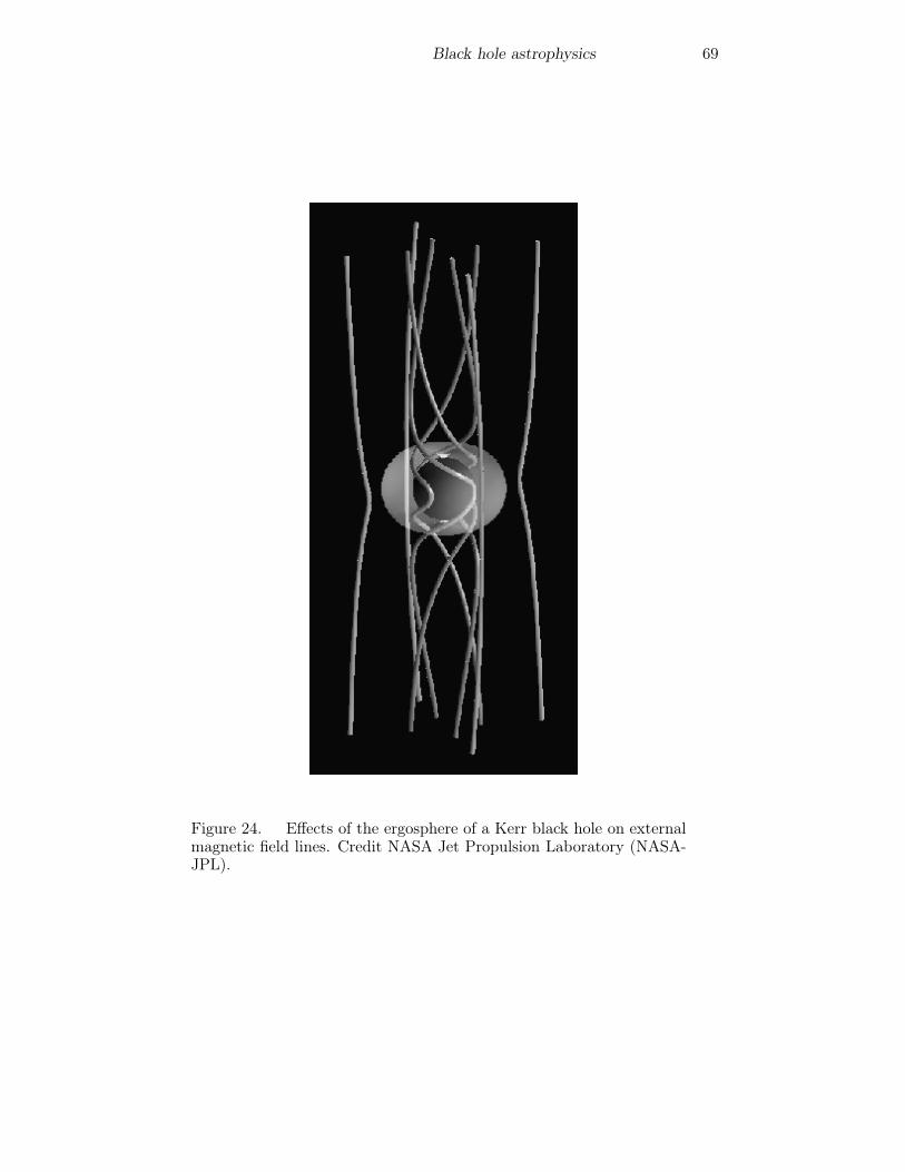
Black hole astrophysics 69
Figure 24. Effects of the ergosphere of a Kerr black hole on externalmagnetic field lines. Credit NASA Jet Propulsion Laboratory (NASA-JPL).
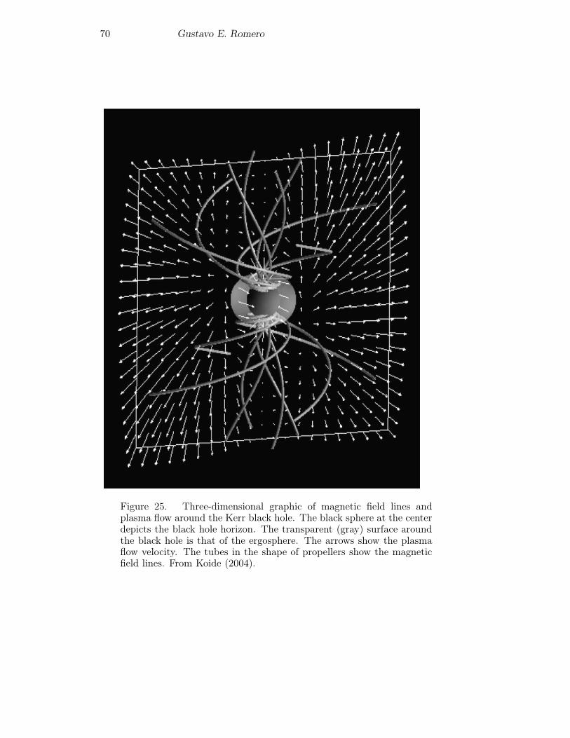
70 Gustavo E. Romero
Figure 25. Three-dimensional graphic of magnetic field lines andplasma flow around the Kerr black hole. The black sphere at the centerdepicts the black hole horizon. The transparent (gray) surface aroundthe black hole is that of the ergosphere. The arrows show the plasmaflow velocity. The tubes in the shape of propellers show the magneticfield lines. From Koide (2004).

Black hole astrophysics 71
Figure 26. Black hole magnetosphere (corona) and resulting outflows.From Koide et al. (1999).
axis perpendicular to the event horizon. The trajectory of photons is given by:
dr
dt= ∓c
∣∣∣∣1− rSchwr
∣∣∣∣ , (258)
with r always decreasing. The light cones are thinner and thinner as r gets closerto the singularity at r = 0. In addition to infalling particles, there is a smallflux of gravitational radiation into the black hole through the horizon becauseof small perturbations outside it. This radiation, as the material particles andphotons, ends in the singularity.
In the case of a Kerr black hole, between the two horizons space and timealso exchange roles as it happens with the Schwarzschild interior black hole space-time. Instead of time always moving inexorably onward, the radial dimension ofspace moves inexorably inward to the second horizon, that it is also a Cauchyhorizon, i.e. a null hyper-surface beyond which predictability breaks down. Afterthat, the Kerr solution predicts a second reversal so that one can avoid thering singularity and achieve to orbit safely. In this strange region inside theCauchy horizon the observer can, by selecting a particular orbit around the ringsingularity, travel backwards in time and meet himself, i.e. there are closed time-like curves. Another possibility admitted by the equations for the observer inthe central region is to plunge through the hole in the ring to emerge in an anti-gravity universe, whose physical laws would be even most peculiar. Or he cantravel through two further horizons, (or more properly anti-horizons), to emergeat coordinate time t = ∞ into some other universe. All this can be representedin a Penrose-Carter diagram for a Kerr black hole (see Figure 27).
All the above discussion on Kerr black hole interiors is rather academic, sincein real black holes the inner horizon is likely unstable. Poisson and Israel (1990)have shown that when the space-time is perturbed by a fully non-linear, ingoing,spherically-symmetric null shell, a null curvature singularity develops at the innerhorizon. This singularity is “weak” in the sense that none the scalar curvatureinvariants is divergent there. The singularity development at the Cauchy horizon
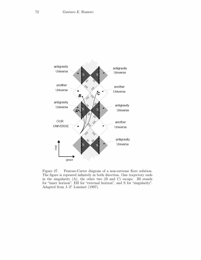
72 Gustavo E. Romero
Figure 27. Penrose-Carter diagram of a non-extreme Kerr solution.The figure is repeated infinitely in both direction. One trajectory endsin the singularity (A), the other two (B and C) escape. IH standsfor “inner horizon”, EH for “external horizon”, and S for “singularity”.Adapted from J.-P. Luminet (1997).
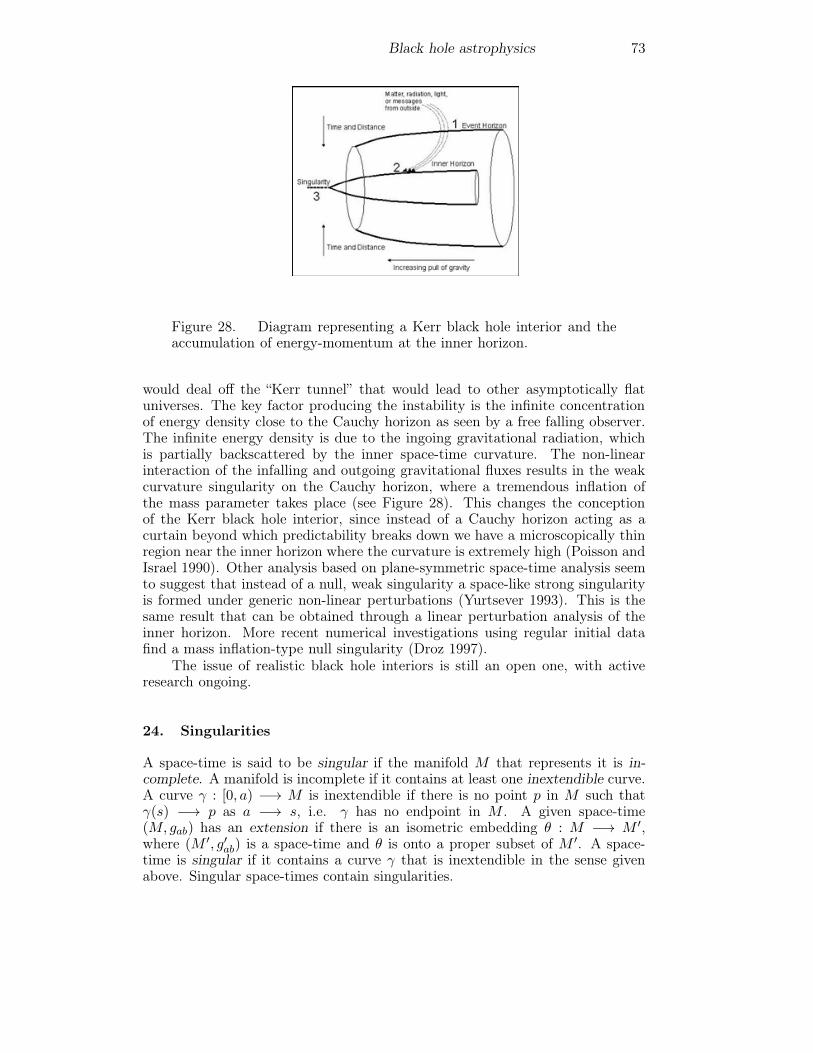
Black hole astrophysics 73
Figure 28. Diagram representing a Kerr black hole interior and theaccumulation of energy-momentum at the inner horizon.
would deal off the “Kerr tunnel” that would lead to other asymptotically flatuniverses. The key factor producing the instability is the infinite concentrationof energy density close to the Cauchy horizon as seen by a free falling observer.The infinite energy density is due to the ingoing gravitational radiation, whichis partially backscattered by the inner space-time curvature. The non-linearinteraction of the infalling and outgoing gravitational fluxes results in the weakcurvature singularity on the Cauchy horizon, where a tremendous inflation ofthe mass parameter takes place (see Figure 28). This changes the conceptionof the Kerr black hole interior, since instead of a Cauchy horizon acting as acurtain beyond which predictability breaks down we have a microscopically thinregion near the inner horizon where the curvature is extremely high (Poisson andIsrael 1990). Other analysis based on plane-symmetric space-time analysis seemto suggest that instead of a null, weak singularity a space-like strong singularityis formed under generic non-linear perturbations (Yurtsever 1993). This is thesame result that can be obtained through a linear perturbation analysis of theinner horizon. More recent numerical investigations using regular initial datafind a mass inflation-type null singularity (Droz 1997).
The issue of realistic black hole interiors is still an open one, with activeresearch ongoing.
24. Singularities
A space-time is said to be singular if the manifold M that represents it is in-complete. A manifold is incomplete if it contains at least one inextendible curve.A curve γ : [0, a) −→ M is inextendible if there is no point p in M such thatγ(s) −→ p as a −→ s, i.e. γ has no endpoint in M . A given space-time(M,gab) has an extension if there is an isometric embedding θ : M −→ M ′,where (M ′, g′ab) is a space-time and θ is onto a proper subset of M ′. A space-time is singular if it contains a curve γ that is inextendible in the sense givenabove. Singular space-times contain singularities.
74 Gustavo E. Romero
A so-called coordinate singularity is not as real singularity. It seems to besingular in some space-time representation but it can be removed by a coordinatechange, like the “Schwarzschild singularity” at rScwh = 2GM/c2 in a Schwarzchildspace-time. We can change to Eddington-Finkelstein coordinates, for instance,and then we see that geodesic lines can go through that point of the manifold.Essential singularities cannot be removed in this way. This occurs, for instance,with the singularity at r = 0 in the Schwarzschild space-time or with the ringsingularity at r = 0 and θ = π/2 in the Kerr metric written in Boyer-Lindquistcoordinates11. In such cases, the curvature scalar RμνρσRμνρσ diverges. There isno metric there, and the Einstein equations cannot be defined.
An essential or true singularity should not be interpreted as a representationof a physical object of infinite density, infinite pressure, etc. Since the singularitydoes not belong to the manifold that represents space-time in General Relativity,it simply cannot be described or represented in the framework of such a theory.General Relativity is incomplete in the sense that it cannot provide a full de-scription of the gravitational behavior of any physical system. True singularitiesare not within the range of values of the bound variables of the theory: they donot belong to the ontology of a world that can be described with 4-dimensionaldifferential manifolds.
An essential singularity in solutions of the Einstein field equations is one oftwo things:
1. A situation where matter is forced to be compressed to a point (a space-likesingularity).
2. A situation where certain light rays come from a region with infinite cur-vature (time-like singularity).
Space-like singularities are a feature of non-rotating uncharged black-holes, whereastime-like singularities are those that occur in charged or rotating black hole exactsolutions, where time-like or null curves can always avoid hitting the singularities.
Singularities do not belong to classical space-time. This is not surprisingsince singularities are extremely compact systems. At such small scales, relationsamong things should be described in a quantum mechanical way. If space-timeis formed by the events that occur to things, it should be represented throughquantum mechanic theory when the things are described by a quantum theory.Since even in the standard quantum theory time appears as a continuum variable,a new approach is necessary.
Space-time singularities are expected to be covered by horizons. Althoughformation mechanisms for naked singularities have been proposed, the followingconjecture is usually considered valid:
• Cosmic Censorship Conjecture (Roger Penrose): Singularities are alwayshidden behind event horizons.
We emphasize that this conjecture is not proved in General Relativity andhence it has not the strength of a theorem of the theory.
11In Cartesian coordinates the Kerr singularity occurs at x2 + y2 = a2c−2 and z = 0.
Black hole astrophysics 75
The classical references on singularities are Hawking and Ellis (1973) andClarke (1993).
Singularity theorems
Several singularity theorems can be proved from pure geometrical properties ofthe space-time model (Clarke 1993). The most important one is due to Hawking& Penrose (1970):
Theorem. Let (M, gab) a time-oriented space-time satisfying the followingconditions:
1. RabVaV b ≥ 0 for any non space-like V a.
2. Time-like and null generic conditions are fulfilled.
3. There are no closed time-like curves.
4. At least one of the following conditions holds
• There exists a compact12 achronal set13 without edge.• There exists a trapped surface.• There is a p ∈ M such that the expansion of the future (or past)
directed null geodesics through p becomes negative along each of thegeodesics.
Then, (M, gab) contains at least one incomplete time-like or null geodesic.
The theorem is purely geometric, no physical law is invoked. If the theoremhas to be applied to the physical world, the hypothesis must be supported byempirical evidence. Condition 1 will be satisfied if if the energy-momentumT ab satisfies the so-called strong energy condition: Tabξaξb ≥ −(1/2)T a
a , for anytime-like vector ξa. If the energy-momentum is diagonal: Tμμ = (ρ,−p,−p,−p)the strong enegy condition can be written as: ρ + 3p ≥ 0 and ρ + p ≥ 0.Condition 2 requires that any time-like or null geodesic experiences a tidal forceat some point in its history. Condition 4a requires that, at least at one time,
12A space is said to be compact if whenever one takes an infinite number of "steps" in the space,eventually one must get arbitrarily close to some other point of the space. Thus, whereas disksand spheres are compact, infinite lines and planes are not, nor is a disk or a sphere with amissing point. In the case of an infinite line or plane, one can set off making equal steps in anydirection without approaching any point, so that neither space is compact. In the case of a diskor sphere with a missing point, one can move toward the missing point without approaching anypoint within the space. More formally, a topological space is compact if, whenever a collectionof open sets covers the space, some subcollection consisting only of finitely many open sets alsocovers the space. A topological space is called compact if each of its open covers has a finitesubcover. Otherwise it is called non-compact. Compactness, when defined in this manner,often allows one to take information that is known locally – in a neighborhood of each pointof the space – and to extend it to information that holds globally throughout the space.
13A set of points in a space-time with no two points of the set having time-like separation.
76 Gustavo E. Romero
the universe is closed and the compact slice that corresponds to such a timeis not intersected more than once by a future directed time-like curve. Thetrapped surfaces mentioned in 4b refers to horizons due to gravitational collapse.Condition 4c requires that the universe is collapsing in the past or the future.
A closely related theorem is due to Hawking (1967):
Theorem. Let (M, gab) a time-oriented space-time satisfying the followingconditions:
1. RabVaV b ≥ 0 for any non space-like V a.
2. There exists a compact space-like hypersurface Σ ⊂M without edge.
3. The unit normals to Σ are everywhere converging (or diverging).
Then, (M, gab) is time-like geodesically incomplete.
Although singularity theorems apply to spherically symmetric black holes,they do not seem to apply to the Universe as a whole.
25. Accretion onto black holes
Accretion is the process of matter falling into the potential well of a gravitatingobject. The accretion of matter which does not have angular momentum isbasically determined by the relation between the sound speed as in the matterand the velocity of the object respect to the medium vrel (Bondi & Hoyle 1944).The accretion of matter with angular momentum can lead to the formation of anaccretion disk around the compact object (Shakura & Sunyaev 1973). In whatfollows, we will discuss the fluid dynamics of accretion onto a black hole.
The are four basic regimes of accretion onto a black hole:
• Spherical symmetric accretion. It occurs when vrel << as and the accretingmatter does not have any significant angular momentum.
• Cylindrical accretion. The angular momentum of the medium remainssmall but now vrel ≥ as.
• Disk accretion. The total angular momentum of matter is enough as toform an accretion disk around the black hole.
• Two-stream accretion. Both a quasi-spherically symmetric inflow of mattercoexists with disk accretion (e.g. Narayan & Yi 1994).
The fluid dynamic description of a physical process is applicable if the freemean path for particles in the medium is much shorter than the typical size-scaleof the system. In the case of accretion, the self-gravitation of the accreting matteris usually negligible, so the characteristic length is the gravitational captureradius RG. This quantity is equal to the distance at which the kinetic energy ofthe matter is of the order of the gravitational energy:
1
2(a2s + v2rel) =
GM
RG.

Black hole astrophysics 77
Here, M is the mass of the accreting object. Hence,
RG =2GM
a2s + v2rel. (259)
In the absence of radiation, the equations that fully describe the accretionprocess are:
∂�v
∂t+ �v �∇�v = −1
ρ�∇P − �∇φ, (260)
∂ρ
∂t+ �∇(ρ�v) = 0, (261)
P = P (ρ), (262)
∇2φ = −4πGρtot. (263)
Equation (260) is the non-relativistic Euler’s equation in a gravitational field ofpotential φ, with P being the fluid pressure and ρ its density. Equation (315) isthe continuity equation. The third equation is the equation of state of the fluid.The final equation is Poisson’s equation for the gravitational potential producedby the total mass density of the system. By the moment we assume non-radiativeand non-relativistic accretion.
The accretion rate onto the black hole will be:
M = σGρvrel, (264)
where σG is the cross section of gravitational capture. This cross section stronglydepends on the nature of the gas. If the gas is formed by collisionless particles,these can be captured only if they have an impact parameter smaller than thesize of the compact object, whereas if the gas is a continuous media, angular mo-mentum is not conserved and essentially all particles with kinetic energy smallerthan the gravitational energy will be captured. Considering a Schwarzschildblack hole, then, we have:
σG(collisionless)
σG(continuous)=RSchw
RG<< 1. (265)
Under typical conditions in the interstellar medium the accretion of fluid is abouta million times the accretion of collisionless particles. The accretion rate of Eq.(264) can be written is the case of fluid dynamics as:
M = πR2Gρvrel. (266)
25.1. Spherically symmetric accretion
Bondi (1952) was the first to obtain the stationary spherically symmetric solutionof Eqs (260-263), assuming an adiabatic equation of state P ∝ ργ . The Eulerequation implies the conservation of energy:
v2
2+
γ
γ − 1
P
ρ− GM
R= constant = ε0. (267)
78 Gustavo E. Romero
The continuity equation can written as:
M = 4πR2ρv = constant, (268)
where we have considered accretion over a sphere of radius R.The boundary conditions at infinity imply:
ε0 =γ
γ − 1
P∞ρ∞
=a2∞γ − 1
. (269)
The speed of sound is
as =
öP
∂ρ=
√γP
ρ.
Then,v2
2+
a2sγ − 1
=GM
R+
a2∞γ − 1
, (270)
and
v =M
4πρ∞R
(a∞as
)2/(γ−1)
. (271)
There is a critical point at R = Rs which the gas velocity overcomes thespeed of the sound. At R << Rs the matter is practically in a state of free falltoward the black hole. This is because of the flow becomes supersonic and thenthe underlying layers do not do not affect the entrained matter. Then, we canwrite:
v ≈√
2GM
R, (272)
and
ρ ≈ M
4π√2GM
R−3/2. (273)
If the effect of radiation is going to be taken into account, then we add thesecond law of thermodynamics to Eqs. (260-263). The energy variation per unitmass is:
dε = −PdV + dQ, (274)
where V is the specific gas volume and dQ is the heat released by unit mass. Forthe case of a monoatomic gas or a fully ionized plasma, we have:
3
2μRu
dT
dt= Ru
T
μρ
dρ
dt− αffT
1/2ρ+dQ
dt. (275)
Here, Ru is the universal gas constant, the second term on the right is due toBremsstrahlung losses (αff ≈ 5 × 10²⁰ erg g−1 s−1), and the third term takesinto account other possible radiation losses. Using vdt = dR and reminding that
Black hole astrophysics 79
ρ ∝ R−3/2, we can obtain the equation for the temperature distribution in asteady state spherically symmetric accretion flow:
dT
dR= −T
R+ constant
√T
R+
2μ
3Ru
dQ
dR. (276)
Notice that if there are no additional radiation losses besides free-free radiation(dQ/dR = 0), Eq. (276) can be solved to obtain
T =
[K ln
(R
RG
)+ T 1/2
∞]2, (277)
where we have assumed that at R = RG the matter temperature is T∞. Eq.(277) shows that under such conditions the temperature decreases as the flowapproaches to the black hole. A fluid that behaves in this way is called a coolingflow.
The radial free fall time is:
tfall ≈ R
vR∝ R3/2, (278)
whereas the cooling time for free-free losses (dQ/dT ∝ T 1/2ρ) is14:
tcool =3RuT
2dQ/dt∝
√T
ρ≈ R. (279)
Comparing both equations we see that the relative role of cooling decreases asthe black hole is approached.
Close to the black hole, however, there could be sources of radiation, ifmagnetic field and angular momentum are involved. The outgoing radiation willpass through the accretion flow and can influence its dynamics. Let σ be thecross section of interaction of the emitted radiation with matter.The force actingupon the infalling particles is:
Frad =σL
4πR2c, (280)
where L is the luminosity of the radiation. The attractive gravitational force ona particle of mass mp is:
Fgrav =GMmp
R2, (281)
with M the mass of the black hole. For a luminosity L = LEdd these forces arebalanced and spherical accretion is stopped:
LEdd =4πMmpc
σ. (282)
14Notice that T ∝ R−1 and ρ ∝ R3/2.
80 Gustavo E. Romero
This critical luminosity is called the Eddington luminosity of the accreting source.In the case of Thomson scattering σ = σT ≈ 0.66×10⁻²⁴ cm2, and we can write:
LEdd ≈ 1.3× 1038(M
M�
)erg s−1. (283)
Associated with the Eddington luminosity we have a critical accretion rate:
MEdd =LEdd
c2≈ 0.2× 10⁻⁸
(M
M�
)M� yr−1. (284)
The Eddington temperature TEdd is the characteristic black body temperaturerequired for a body with the Schwarzschild radius to radiate LEdd:
TEdd =
(LEdd
4πσSBR2Schw
)≈ 6.6× 10⁷
(M
M�
)−1/4
K. (285)
Another way to inhibit spherical accretion is the production of winds orparticle ejection in the inner accreting regions. If Lej is the power carried awayby the ejected particles and vej is their velocity, the exerted pressure will be:
Pej =Lej
4πR2vej. (286)
If the central source ejects particles before the onset of the spherical accre-tion, pressures must be equated at the gravitational capture radius to find thecritical luminosity in ejected particles:
Lej
4πR2Gvej
= ρv2∞ =M
4πR2G
v∞.
From here we get:Lcritej = Mv∞vej. (287)
Using the fact that a fraction η of the accretion power is released as radiation,i.e.
L = η ˙Mc2, (288)
we obtainLcritej =
L
η
(v∞vejc2
). (289)
It can be seen that a weak wind can stop the the spherical accretion.
25.2. Cylindrical accretion
The problem of cylindrical accretion is the problem of the determination of thegas accretion onto a moving gravitating center. Unlike the case of sphericalaccretion, the problem is quite complex and there are not analytical solutionsof it. In cylindrical accretion, the velocity of the compact object respect to themedium vrel is not negligible. In order to deal with the problem is convenient toadopt a coordinate system centered in the moving object. The symmetry axis of
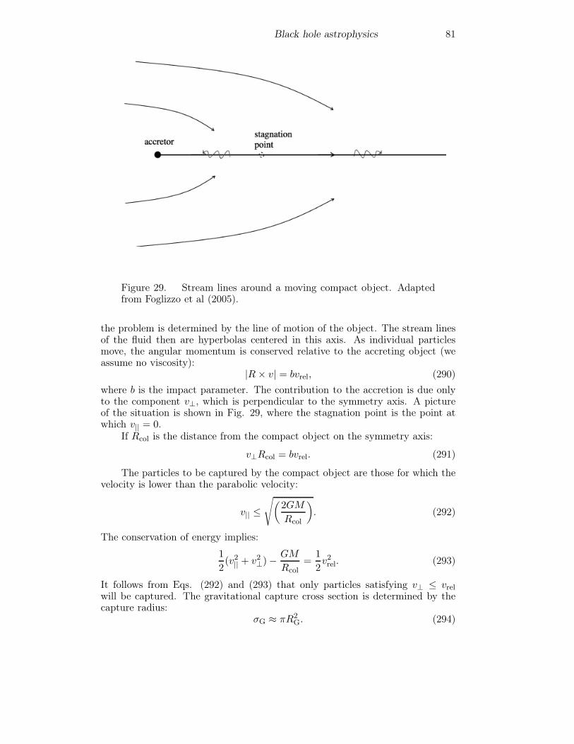
Black hole astrophysics 81
Figure 29. Stream lines around a moving compact object. Adaptedfrom Foglizzo et al (2005).
the problem is determined by the line of motion of the object. The stream linesof the fluid then are hyperbolas centered in this axis. As individual particlesmove, the angular momentum is conserved relative to the accreting object (weassume no viscosity):
|R× v| = bvrel, (290)where b is the impact parameter. The contribution to the accretion is due onlyto the component v⊥, which is perpendicular to the symmetry axis. A pictureof the situation is shown in Fig. 29, where the stagnation point is the point atwhich v|| = 0.
If Rcol is the distance from the compact object on the symmetry axis:
v⊥Rcol = bvrel. (291)
The particles to be captured by the compact object are those for which thevelocity is lower than the parabolic velocity:
v|| ≤√(
2GM
Rcol
). (292)
The conservation of energy implies:
1
2(v2|| + v2⊥)−
GM
Rcol=
1
2v2rel. (293)
It follows from Eqs. (292) and (293) that only particles satisfying v⊥ ≤ vrelwill be captured. The gravitational capture cross section is determined by thecapture radius:
σG ≈ πR2G. (294)
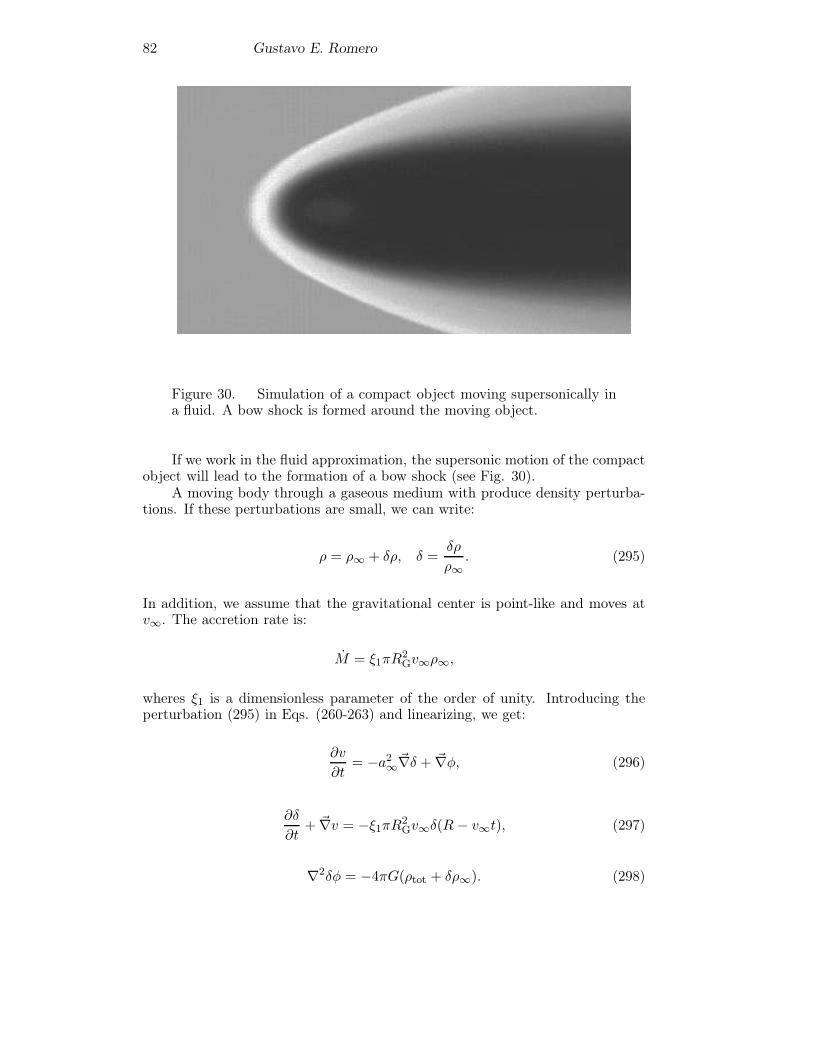
82 Gustavo E. Romero
Figure 30. Simulation of a compact object moving supersonically ina fluid. A bow shock is formed around the moving object.
If we work in the fluid approximation, the supersonic motion of the compactobject will lead to the formation of a bow shock (see Fig. 30).
A moving body through a gaseous medium with produce density perturba-tions. If these perturbations are small, we can write:
ρ = ρ∞ + δρ, δ =δρ
ρ∞. (295)
In addition, we assume that the gravitational center is point-like and moves atv∞. The accretion rate is:
M = ξ1πR2Gv∞ρ∞,
wheres ξ1 is a dimensionless parameter of the order of unity. Introducing theperturbation (295) in Eqs. (260-263) and linearizing, we get:
∂v
∂t= −a2∞�∇δ + �∇φ, (296)
∂δ
∂t+ �∇v = −ξ1πR2
Gv∞δ(R − v∞t), (297)
∇2δφ = −4πG(ρtot + δρ∞). (298)
Black hole astrophysics 83
Using the Jeans wavelength15 (Zeldovich & Novikov 1971):
k2J =4πGρ∞a2∞
, (299)
we can cast Eqs. (296-297) in the following form of an equation in the pertur-bations produced by the moving gravitational center:
�2δ + k2Ja2∞δ = −4πGρtot + ξ1πR
2Gv∞
∂
∂tδ(R − v∞t). (300)
To simplify Eq. (300), we can center the center the coordinate system inthe moving object and neglect self-gravity of the gas (kJ). Then, (300) can bewritten as:
(a2∞ − v2∞)∇2δ = 4πGMδ(R). (301)The solution is (Lipunov 1992):
δ =RGv∞
a∞R(1− v2∞
a2∞ sin2 θsh
)1/2 . (302)
If we introduce the Mach number MM = v∞/a∞, we see from Eq. (302)that there is a singularity at the surface of the cone described by:
sin θsh =1
MM. (303)
This means that the solution (302) is not valid close to the cone, which impliesthat a shock wave is formed, with a form of a cone with opening angle θsh (seeFig. 30). This shock is called a “bow shock”.
A force due to dynamical friction opposes to the motion of the compactobject, slowing it down. Such a force is the result that the density in the back-ground matter in the wake is higher than in front of the moving center. Thedynamic friction force is:
Ffr = πR2Gρ∞v∞. (304)
Numerical simulations show that the accretion flow pattern is complicatedand dependent on the efficiency of the gas cooling mechanism. The simulationsalso show the formation of a frontal shock at a distance ∼ RG. This region isprone to suffer Reyleight-Taylor instabilities (e.g. Araudo et al. 2009). In Fig.31 we show a 3D Smooth Particle Hydrodynamic (SPH) simulation of a movingblack hole in a stellar wind.
The temperature in the wake of the the shock is (Lang 1999):
Tsh =mpv
2∞6k
≈ 2.5× 10⁵(
v∞107 cm s−1
)2
K, (305)
where k is the Boltzmann’s constant.A realistic study of the accretion regimes onto moving objects requires ex-
tensive numerical simulations.
15The Jeans wavelength kJ is defined such that any small sinusoidal density disturbance with awavelength exceeding 2π/kJ will be gravitationally unstable. The Jeans critical mass is usuallydefined as the density times the cubic of the length. Higher masses than the Jeans mass startto condense gravitationally.
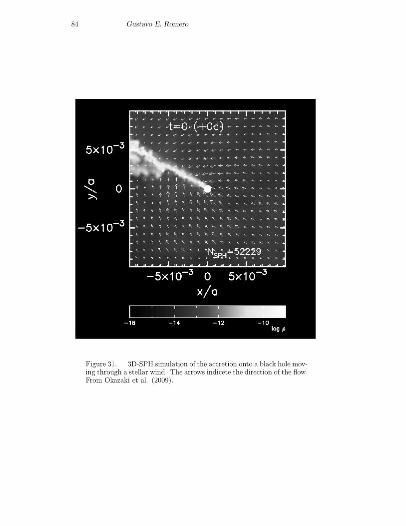
84 Gustavo E. Romero
Figure 31. 3D-SPH simulation of the accretion onto a black hole mov-ing through a stellar wind. The arrows indicete the direction of the flow.From Okazaki et al. (2009).
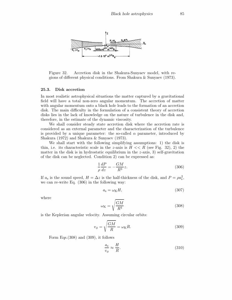
Black hole astrophysics 85
Figure 32. Accretion disk in the Shakura-Sunyaev model, with re-gions of different physical conditions. From Shakura & Sunyaev (1973).
25.3. Disk accretion
In most realistic astrophysical situations the matter captured by a gravitationalfield will have a total non-zero angular momentum. The accretion of matterwith angular momentum onto a black hole leads to the formation of an accretiondisk. The main difficulty in the formulation of a consistent theory of accretiondisks lies in the lack of knowledge on the nature of turbulence in the disk and,therefore, in the estimate of the dynamic viscosity.
We shall consider steady state accretion disk where the accretion rate isconsidered as an external parameter and the characterization of the turbulenceis provided by a unique parameter: the so-called α parameter, introduced byShakura (1972) and Shakura & Sunyaev (1973).
We shall start with the following simplifying assumptions: 1) the disk isthin, i.e. its characteristic scale in the z-axis is H << R (see Fig. 32), 2) thematter in the disk is in hydrostatic equilibrium in the z-axis, 3) self-gravitationof the disk can be neglected. Condition 2) can be expressed as:
1
ρ
dP
dz= −GM
R3z. (306)
If as is the sound speed, H = Δz is the half-thickness of the disk, and P = ρa2s ,we can re-write Eq. (306) in the following way:
as = ωKH, (307)
where
ωK =
√GM
R3(308)
is the Keplerian angular velocity. Assuming circular orbits:
vφ =
√GM
R= ωKR. (309)
Form Eqs.(308) and (309), it follows
asvφ
≈ H
R. (310)
86 Gustavo E. Romero
Notice that since the particles move into Keplerian orbits there is no pres-sure gradient along R. The transport of angular momentum along the disk isassociated with the moment of viscous forces:
MdωK
dRR2 = 2π
d
dRWrφR
2. (311)
Here, Wrφ is the component of the viscous stress in the disk:
Wrφ = −2ηHR∂ωK
∂R. (312)
The parameter η is the dynamic viscosity averaged over the z-coordinate. Noticethat for a rigid body ∂ωK/∂R = 0 and the viscous stress vanishes.
The viscosity of isotropic turbulence is (Landau & Lifshitz 2002): η =(1/3)ρvtlt, where vt and lt are the characteristic velocity and scale of the tur-bulence, respectively. Shakura (1972) introduced the following expression tocharacterize the viscous fluid:
vtlt = αasH, (313)
where α is the viscosity parameter. Since vt < as16 and lt < H, then α ≤ 1.
Equation (311) can be integrated yielding:
Wrφ = −M2πωK
[1−
(Rd
R
)1/2]+Wrφ(in), (314)
where Rd is the radius of the inner edge of the disk and Wrφ(in) is the componentof the tensor of viscous stress evaluated at R = Rd. As we have seen before, fora Schwarzschild black hole the last stable orbit is at Rd = 3RSchw. For this lastorbit, we can take:
Wrφ(in) = 0.
The continuity equation can be written as:
M = 2πρ(2H)RvR, (315)
with vR the radial velocity of the matter in the accretion disk.Far from the inner edge we have:
Wrφ ≈ −M2πωK ≈ 3ηHωK = αPH. (316)
From this equation and eq. (315) it can be obtained that
vRvφ
≈ α
(H
R
)2
. (317)
16Turbulence is quickly attenuated in supersonic flows.
Black hole astrophysics 87
The transport of angular momentum in the disk results in the generationof heat. We can express the heat produced per unit surface area of the disk perunit of time on each side as:
Q+ = −1
2WrφR
dω
dR=
3
4ωWrφ. (318)
This energy is carried away in the form of thermal radiation:
Q− = σSBT4, (319)
where σSB is the Stephan-Boltzmann’s constant and we have assumed that thedisk radiates as a black body. In the steady state Q+ = Q−. If Q+ > Q− thedisk becomes thermally unstable. The full set of equations that determine thedisk accretion are:
1. ω = ωK =(GMR3
)1/2(Kepler’s law).
2. M = −2πΣvRR (continuity equation).
3. Wrφ = − M2πωK
[1−
(RdR
)1/2]+Wrφ(in) (variation of angular momentum).
4. P = Σω2H6 (hydrostatic equilibrium).
5. Wrφ = αPH (viscous tensor).
6. Q+ = −12WrφR
dωdR (energy release).
7. Q− = σSBT4 (losses by radiation).
8. P = 32ρRu(Te + Ti) +
ε3 (equation of state, with ε the energy density).
9. σ[cm2] = σT + σff ≈ 6.65 × 10⁻²⁵n + 1.8×10⁻²⁵
T7/2 (absorption cross section).
This is a system of 9 equations with 9 functions of R as solution. Thesolutions where found by Shakura & Sunyaev (1973). For fixed values of M andM , the disk can be into three different regions:
• An outer region (large R) where the gas pressure dominates over radiationpressure and opacity is controlled by free-free absroption.
• A middle region (smaller R) where the gas pressure dominates over radia-tion pressure but the opacity is due to electron scattering.
• An inner region (very small R) where radiation pressure dominates overgas pressure and the opacity is also due to electron scattering.
88 Gustavo E. Romero
Luminosity and spectrum of standard accretion disks
The energy carried with the radiation released in a ring of thickness dR of theaccretion disk is:
dL(R) = 2Q+2πRdR, (320)
where the initial factor 2 is due to the two faces of the disk. This equation canbe written as:
dL(R) =3
2M
d
dR
GM
R2
⎛⎝1−√Rd
R
⎞⎠ dR. (321)
The power dL(R) corresponds to the work done by the gravitational field.Approximately half of this power is transformed into kinetic energy of the mattermoving along φ and the other half is transformed into heat:
dLgr = Md
dr
(−GM
2R
)dR =
1
2MGM
R2dR. (322)
Comparing Eqs. (321) and (322) we see that at large distances from theinner edge the dissipation rate is three times larger than the gravitational energyrelease. This is because of th viscous effects, the half of the gravitational energyis radiated from the disk globally but not locally. The total luminosity of the diskis:
Ld =
∫ ∞
Rd
dL(R)
dRdR =
MGM
2R. (323)
Adopting Rd = 3RSchw and dividing by Mc2 we get the efficiency of energyrelease in the disk accretion process: ∼ 8 %. For a Kerr black hole, whereRd = Rg, the efficiency reaches ∼ 42 %.
Using Eq. (321) we get:
Q+ =3
8π
MGM
R3, (324)
for R >> Rd. Through the energy energy balance equation Q+ = Q− = σSBT4
we can obtain the temperature distribution along the radial direction in the disk:
T (R) =
(3
8πσSBMGM
R3
)1/4
∝ R−3/4. (325)
The total spectrum is the result of the superposition of the blackbody emis-sion from each ring of temperature T (R):
Iν = 2π
∫ Rout
Rd
Bν [T (R)]RdR, (326)
with
Bν(T ) =2πh
c2
(kT
h
)3 x3
ex − 1; x ≡ hv
kT, (327)
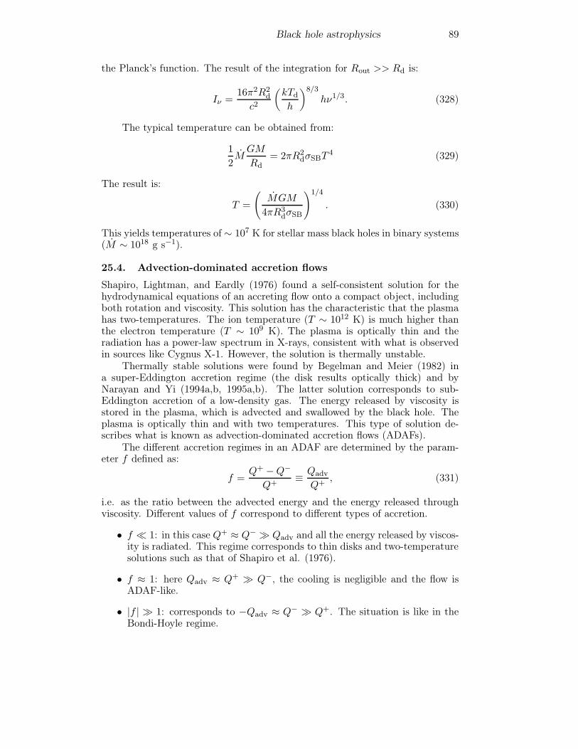
Black hole astrophysics 89
the Planck’s function. The result of the integration for Rout >> Rd is:
Iν =16π2R2
d
c2
(kTdh
)8/3
hν1/3. (328)
The typical temperature can be obtained from:
1
2MGM
Rd= 2πR2
dσSBT4 (329)
The result is:
T =
(MGM
4πR3dσSB
)1/4
. (330)
This yields temperatures of ∼ 107 K for stellar mass black holes in binary systems(M ∼ 1018 g s−1).
25.4. Advection-dominated accretion flows
Shapiro, Lightman, and Eardly (1976) found a self-consistent solution for thehydrodynamical equations of an accreting flow onto a compact object, includingboth rotation and viscosity. This solution has the characteristic that the plasmahas two-temperatures. The ion temperature (T ∼ 1012 K) is much higher thanthe electron temperature (T ∼ 109 K). The plasma is optically thin and theradiation has a power-law spectrum in X-rays, consistent with what is observedin sources like Cygnus X-1. However, the solution is thermally unstable.
Thermally stable solutions were found by Begelman and Meier (1982) ina super-Eddington accretion regime (the disk results optically thick) and byNarayan and Yi (1994a,b, 1995a,b). The latter solution corresponds to sub-Eddington accretion of a low-density gas. The energy released by viscosity isstored in the plasma, which is advected and swallowed by the black hole. Theplasma is optically thin and with two temperatures. This type of solution de-scribes what is known as advection-dominated accretion flows (ADAFs).
The different accretion regimes in an ADAF are determined by the param-eter f defined as:
f =Q+ −Q−
Q+≡ Qadv
Q+, (331)
i.e. as the ratio between the advected energy and the energy released throughviscosity. Different values of f correspond to different types of accretion.
• f � 1: in this case Q+ ≈ Q− � Qadv and all the energy released by viscos-ity is radiated. This regime corresponds to thin disks and two-temperaturesolutions such as that of Shapiro et al. (1976).
• f ≈ 1: here Qadv ≈ Q+ � Q−, the cooling is negligible and the flow isADAF-like.
• |f | � 1: corresponds to −Qadv ≈ Q− � Q+. The situation is like in theBondi-Hoyle regime.
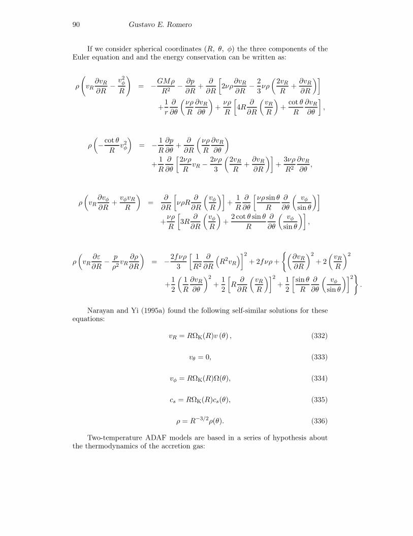
90 Gustavo E. Romero
If we consider spherical coordinates (R, θ, φ) the three components of theEuler equation and and the energy conservation can be written as:
ρ
(vR∂vR∂R
− v2φR
)= −GMρ
R2− ∂p
∂R+
∂
∂R
[2νρ
∂vR∂R
− 2
3νρ
(2vRR
+∂vR∂R
)]+1
r
∂
∂θ
(νρ
R
∂vR∂θ
)+νρ
R
[4R
∂
∂R
(vRR
)+
cot θ
R
∂vR∂θ
],
ρ
(−cot θ
Rv2φ
)= − 1
R
∂p
∂θ+
∂
∂R
(νρ
R
∂vR∂θ
)+
1
R
∂
∂θ
[2νρ
RvR − 2νρ
3
(2vRR
+∂vR∂R
)]+
3νρ
R2
∂vR∂θ
,
ρ
(vR∂vφ∂R
+vφvRR
)=
∂
∂R
[νρR
∂
∂R
(vφR
)]+
1
R
∂
∂θ
[νρ sin θ
R
∂
∂θ
(vφsin θ
)]+νρ
R
[3R
∂
∂R
(vφR
)+
2cot θ sin θ
R
∂
∂θ
(vφsin θ
)],
ρ
(vR
∂ε
∂R− p
ρ2vR
∂ρ
∂R
)= −2fνρ
3
[1
R2
∂
∂R
(R2vR
)]2+ 2fνρ+
{(∂vR∂R
)2
+ 2
(vRR
)2
+1
2
(1
R
∂vR∂θ
)2
+1
2
[R∂
∂R
(vRR
)]2+
1
2
[sin θ
R
∂
∂θ
(vφsin θ
)]2}.
Narayan and Yi (1995a) found the following self-similar solutions for theseequations:
vR = RΩK(R)v (θ) , (332)
vθ = 0, (333)
vφ = RΩK(R)Ω(θ), (334)
cs = RΩK(R)cs(θ), (335)
ρ = R−3/2ρ(θ). (336)
Two-temperature ADAF models are based in a series of hypothesis aboutthe thermodynamics of the accretion gas:
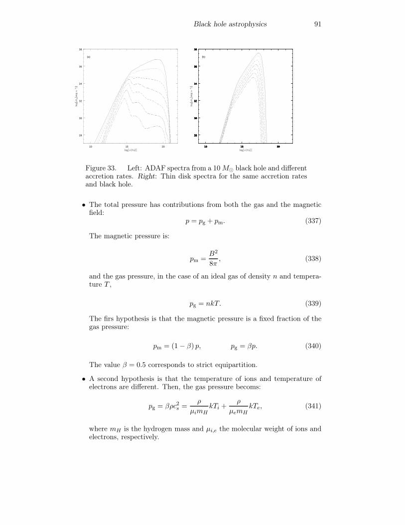
Black hole astrophysics 91
10 15 20
28
30
32
34
36
38
(a)
10 15 20
28
30
32
34
36
38
(b)
10 15 20
28
30
32
34
36
38
10 15 20
28
30
32
34
36
38
10 15 20
28
30
32
34
36
38
10 15 20
28
30
32
34
36
38
10 15 20
28
30
32
34
36
38
10 15 20
28
30
32
34
36
38
Figure 33. Left: ADAF spectra from a 10M� black hole and differentaccretion rates. Right: Thin disk spectra for the same accretion ratesand black hole.
• The total pressure has contributions from both the gas and the magneticfield:
p = pg + pm. (337)
The magnetic pressure is:
pm =B2
8π, (338)
and the gas pressure, in the case of an ideal gas of density n and tempera-ture T ,
pg = nkT. (339)
The firs hypothesis is that the magnetic pressure is a fixed fraction of thegas pressure:
pm = (1− β) p, pg = βp. (340)
The value β = 0.5 corresponds to strict equipartition.
• A second hypothesis is that the temperature of ions and temperature ofelectrons are different. Then, the gas pressure becoms:
pg = βρc2s =ρ
μimHkTi +
ρ
μemHkTe, (341)
where mH is the hydrogen mass and μi,e the molecular weight of ions andelectrons, respectively.

92 Gustavo E. Romero
Quiescent State
Low State
Intermediate State
High State
Very High State
.m
0.5
0.09
0.08
0.01
Figure 34. Geometry of the flux in different spectral states as a func-tion of the accretion rate normalized in Eddington units (Esin et al.1997).
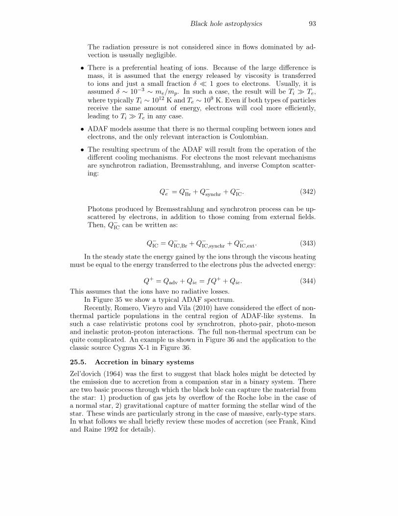
Black hole astrophysics 93
The radiation pressure is not considered since in flows dominated by ad-vection is ussually negligible.
• There is a preferential heating of ions. Because of the large difference ismass, it is assumed that the energy released by viscosity is transferredto ions and just a small fraction δ � 1 goes to electrons. Usually, it isassumed δ ∼ 10−3 ∼ me/mp. In such a case, the result will be Ti � Te,where typically Ti ∼ 1012 K and Te ∼ 109 K. Even if both types of particlesreceive the same amount of energy, electrons will cool more efficiently,leading to Ti � Te in any case.
• ADAF models assume that there is no thermal coupling between iones andelectrons, and the only relevant interaction is Coulombian.
• The resulting spectrum of the ADAF will result from the operation of thedifferent cooling mechanisms. For electrons the most relevant mechanismsare synchrotron radiation, Bremsstrahlung, and inverse Compton scatter-ing:
Q−e = Q−
Br +Q−synchr +Q−
IC. (342)
Photons produced by Bremsstrahlung and synchrotron process can be up-scattered by electrons, in addition to those coming from external fields.Then, Q−
IC can be written as:
Q−IC = Q−
IC,Br +Q−IC,synchr +Q−
IC,ext. (343)
In the steady state the energy gained by the ions through the viscous heatingmust be equal to the energy transferred to the electrons plus the advected energy:
Q+ = Qadv +Qie = fQ+ +Qie. (344)This assumes that the ions have no radiative losses.
In Figure 35 we show a typical ADAF spectrum.Recently, Romero, Vieyro and Vila (2010) have considered the effect of non-
thermal particle populations in the central region of ADAF-like systems. Insuch a case relativistic protons cool by synchrotron, photo-pair, photo-mesonand inelastic proton-proton interactions. The full non-thermal spectrum can bequite complicated. An example us shown in Figure 36 and the application to theclassic source Cygnus X-1 in Figure 36.
25.5. Accretion in binary systems
Zel’dovich (1964) was the first to suggest that black holes might be detected bythe emission due to accretion from a companion star in a binary system. Thereare two basic process through which the black hole can capture the material fromthe star: 1) production of gas jets by overflow of the Roche lobe in the case ofa normal star, 2) gravitational capture of matter forming the stellar wind of thestar. These winds are particularly strong in the case of massive, early-type stars.In what follows we shall briefly review these modes of accretion (see Frank, Kindand Raine 1992 for details).
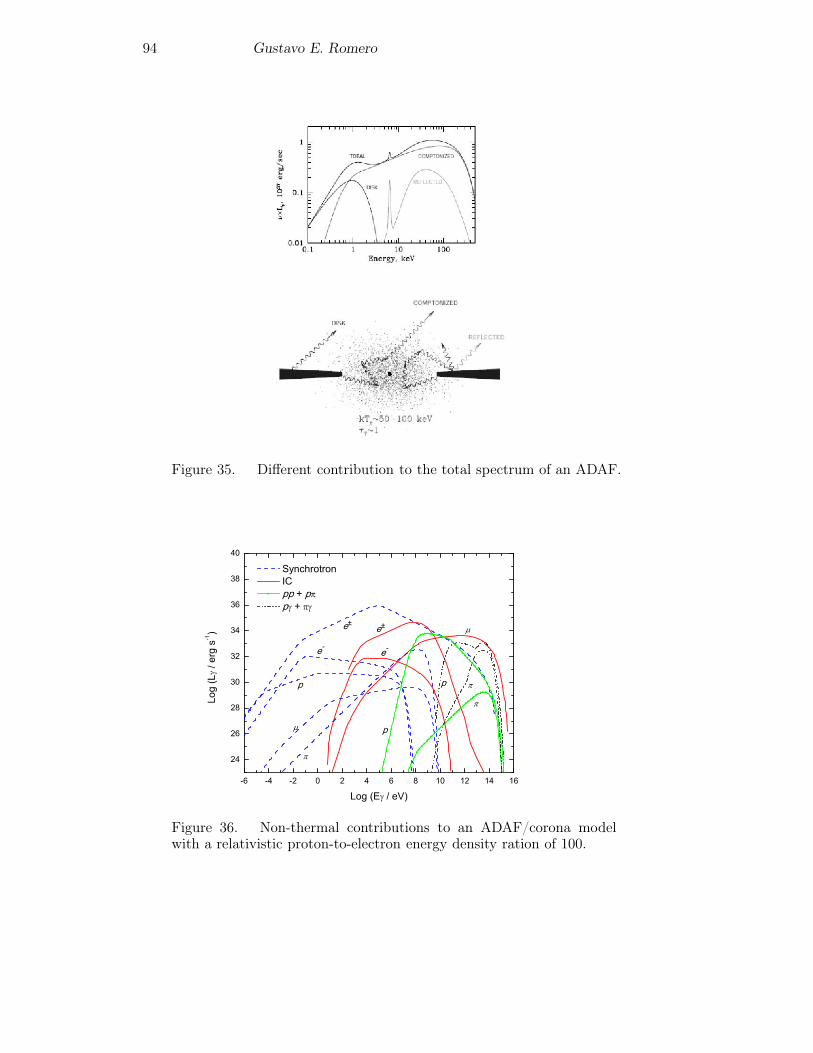
94 Gustavo E. Romero
Figure 35. Different contribution to the total spectrum of an ADAF.
Figure 36. Non-thermal contributions to an ADAF/corona modelwith a relativistic proton-to-electron energy density ration of 100.

Black hole astrophysics 95
Figure 37. ADAF/corona model with non-thermal contribution forCygnus X-1. Different cases are considered, with different proton con-tent.
Overflow of the Roche lobe
Let us consider a black hole of mass M• and a star of mass M∗ in a circular orbit.In the plane of the orbit, the effective potential resulting from the gravitationaland centrifugal forces is (e.g. Lipunov 1992):
Φ = −GM∗R1
− GM•R2
+Ω2(x2 + y2)
2, (345)
where Ω is the angular velocity associated to the radius of the orbit a:
a =
[G(M• +M∗)
Ω2
]1/3, (346)
and R21 = x21 + y21, R2
2 = x22 + y22 indicate the distances of a particle to M∗ andM•, respectively.
The total energy of the particle is:
Φ+1
2v2 = E0. (347)
For low energies, the particle, if emitted by the star, will fall back to it. At theturning point its velocity will be v = 0. In such a case, Φ = E0. This equationdefines equipotential surfaces (Hill’s surfaces) that limit the motion of particlesof energy E0. At a certain energy ER = ΦR, the Hill’s surfaces of both massescome in contact and form the so-called Roche lobe. The point of contact is theinner Lagrangian point where the resultant of all forces equals zero:
dΦ
dx= 0. (348)

96 Gustavo E. Romero
When the star fills its Roche lobe it injects matter over the black holethrough the inner Lagrangian point. There, a particle can go from one lobeto the other without losing energy. The specific angular momentum lΩ of theinjected gas is related to the angular momentum of the orbital motion:
lΩ ≈ Ωa2. (349)
The thickness of the gas jet crossing the Lagrange point is ∼ 0.1 R∗. The flowrate is determined by the state of evolution of the star and the ratio q =M•/M∗.For q � 1, the flow occurs on a time scale
τ =GM∗R∗L∗
, (350)
where L∗ is the total luminosity of the star. Then, the matter flow rate is:
M =M∗τ. (351)
The jet of gas collides with the outer part of the disk. Since the size of thedisk is of the order of the size of the Roche lobe, we can write the time the gastakes to move along the whole disk as:
tR ≈ Rout
vR≈ a
vr≈ a
αvφ(H/R)2≈≈ T
2πα
(R
H
)2
, (352)
where we have used the standard thin disk solution and T is the orbital period.Since for thin disks H � R and α < 1, the time scale of radial motion of matteris longer than the orbital period:
tRT
� 1. (353)
Accretion from stellar winds
The stellar wind of early-type stars is both strong (106 − 10−4 M� yr−1) andsupersonic. The wind velocity is:
vw ≈ vesc ≈√
2GM∗R∗
. (354)
For typical values this velocity will be of a few thousands km s−1, a highlysupersonic value since for the interstellar medium cs ∼ 10 km s−1. If the orbitalvelocity of the black hole in the high-mass binary system is v•, the wind movesforming an angle β = tan−1(v•/vw) with the symmetry axis of the bow shock.The relative velocity is:
vrel = (v2• + v2w)1/2. (355)
Gravitational capture of wind particles will occur within a cylindrical regionof radius
RG ∼ 2GM•v2rel
. (356)
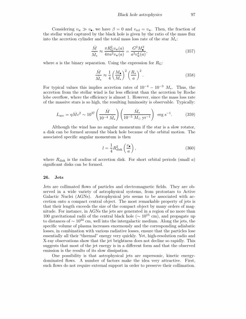
Black hole astrophysics 97
Considering vw � v•, we have β = 0 and vrel = vw. Then, the fraction ofthe stellar wind captured by the black hole is given by the ratio of the mass fluxinto the accretion cylinder and the total mass loss rate of the star M∗:
M
M∗≈ πR2
Gvw(a)
4πa2vw(a)=
G2M2•a2v4w(a)
, (357)
where a is the binary separation. Using the expression for RG:
M
M∗≈ 1
4
(M•M∗
)2 (R∗a
)2
. (358)
For typical values this implies accretion rates of 10−4 − 10−3 M∗. Thus, theaccretion from the stellar wind is far less efficient than the accretion by Rochelobe overflow, where the efficiency is almost 1. However, since the mass loss rateof the massive stars is so high, the resulting luminosity is observable. Typically:
Lacc = ηMc2 ∼ 1037(
M
10−4 M∗
)(M∗
10−5 M� yr−1
)erg s−1. (359)
Although the wind has no angular momentum if the star is a slow rotator,a disk can be formed around the black hole because of the orbital motion. Theassociated specific angular momentum is then
l =1
4R2
disk
(v•a
), (360)
where Rdisk is the radius of accretion disk. For short orbital periods (small a)significant disks can be formed.
26. Jets
Jets are collimated flows of particles and electromagnetic fields. They are ob-served in a wide variety of astrophysical systems, from protostars to ActiveGalactic Nuclei (AGNs). Astrophysical jets seems to be associated with ac-cretion onto a compact central object. The most remarkable property of jets isthat their length exceeds the size of the compact object by many orders of mag-nitude. For instance, in AGNs the jets are generated in a region of no more than100 gravitational radii of the central black hole (∼ 1015 cm), and propagate upto distances of ∼ 1024 cm, well into the intergalactic medium. Along the jets, thespecific volume of plasma increases enormously and the corresponding adiabaticlosses, in combination with various radiative losses, ensure that the particles loseessentially all their “thermal” energy very quickly. Yet, high-resolution radio andX-ray observations show that the jet brightness does not decline so rapidly. Thissuggests that most of the jet energy is in a different form and that the observedemission is the results of its slow dissipation.
One possibility is that astrophysical jets are supersonic, kinetic energy-dominated flows. A number of factors make the idea very attractive. First,such flows do not require external support in order to preserve their collimation.
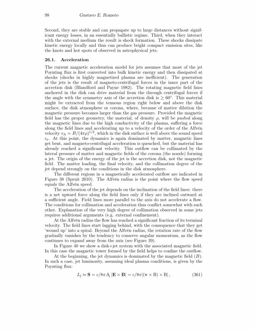
98 Gustavo E. Romero
Second, they are stable and can propagate up to large distances without signif-icant energy losses, in an essentially ballistic regime. Third, when they interactwith the external medium the result is shock formation. These shocks dissipatekinetic energy locally and thus can produce bright compact emission sites, likethe knots and hot spots of observed in astrophysical jets.
26.1. Acceleration
The current magnetic acceleration model for jets assumes that most of the jetPoynting flux is first converted into bulk kinetic energy and then dissipated atshocks (shocks in highly magnetized plasma are inefficient). The generationof the jets is the result of magneto-centrifugal forces in the inner part of theaccretion disk (Blandford and Payne 1982). The rotating magnetic field linesanchored in the disk can drive material from the through centrifugal forces ifthe angle with the symmetry axis of the accretion disk is ≥ 60◦. This materialmight be extracted from the tenuous region right below and above the disksurface, the disk atmosphere or corona, where, because of matter dilution themagnetic pressure becomes larger than the gas pressure. Provided the magneticfield has the proper geometry, the material, of density ρ, will be pushed alongthe magnetic lines due to the high conductivity of the plasma, suffering a forcealong the field lines and accelerating up to a velocity of the order of the Alfvénvelocity vA = B/(4πρ)1/2, which in the disk surface is well above the sound speedcs. At this point, the dynamics is again dominated by matter, magnetic linesget bent, and magneto-centrifugal acceleration is quenched, but the material hasalready reached a significant velocity. This outflow can be collimated by thelateral pressure of matter and magnetic fields of the corona (the nozzle) forminga jet. The origin of the energy of the jet is the accretion disk, not the magneticfield. The matter loading, the final velocity, and the collimation degree of thejet depend strongly on the conditions in the disk atmosphere.
The different regions in a magnetically accelerated outflow are indicated inFigure 38 (Spruit 2010). The Alfvén radius is the point where the flow speedequals the Alfvén speed.
The acceleration of the jet depends on the inclination of the field lines: thereis a net upward force along the field lines only if they are inclined outward ata sufficient angle. Field lines more parallel to the axis do not accelerate a flow.The conditions for collimation and acceleration thus conflict somewhat with eachother. Explanation of the very high degree of collimation observed in some jetsrequires additional arguments (e.g. external confinement).
At the Alfvén radius the flow has reached a significant fraction of its terminalvelocity. The field lines start lagging behind, with the consequence that they get‘wound up’ into a spiral. Beyond the Alfvén radius, the rotation rate of the flowgradually vanishes by the tendency to conserve angular momentum, as the flowcontinues to expand away from the axis (see Figure 39).
In Figure 40 we show a disk+jet system with the associated magnetic field.In this case the magnetic tower formed by the field helps to confine the outflow.
At the beginning, the jet dynamics is dominated by the magnetic field (B).In such a case, jet luminosity, assuming ideal plasma conditions, is given by thePoynting flux:
Lj ≈ S = c/8πAj |E×B| = c/8π|(v × B)× B| , (361)
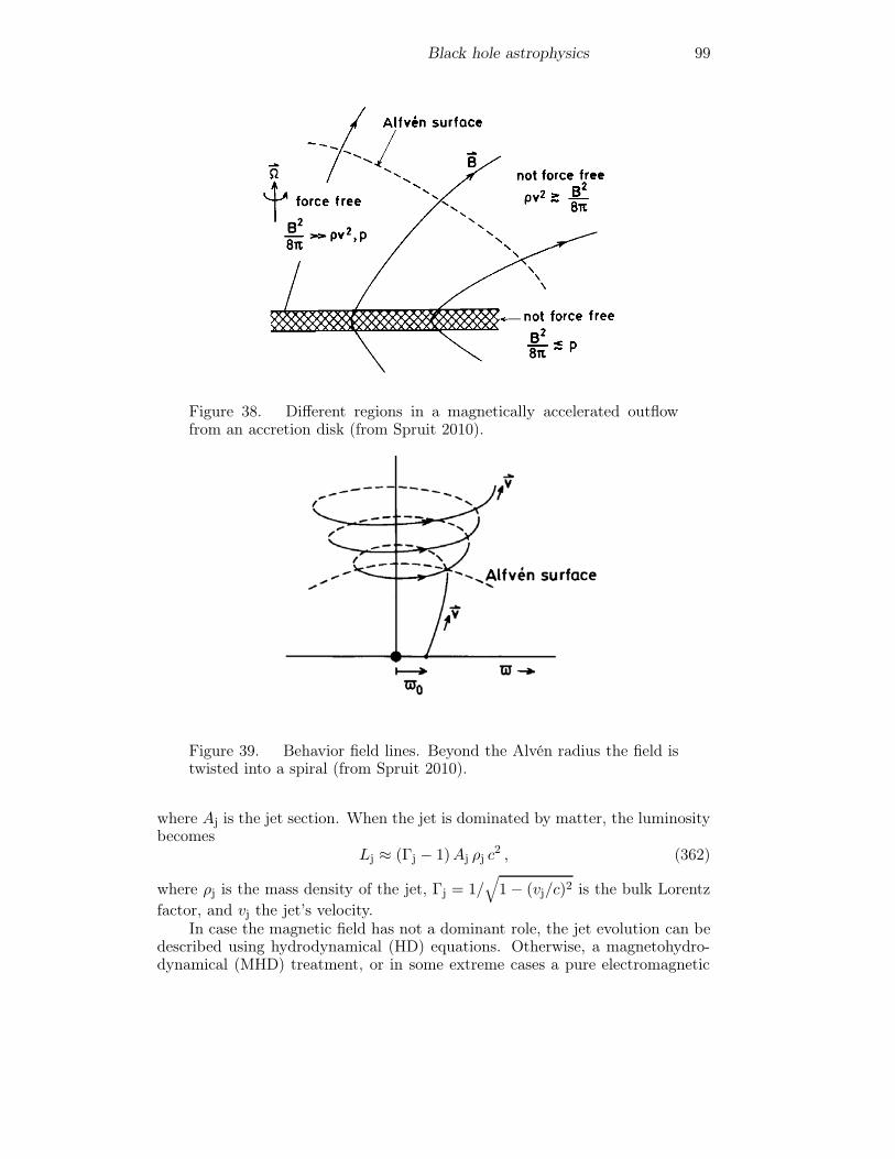
Black hole astrophysics 99
Figure 38. Different regions in a magnetically accelerated outflowfrom an accretion disk (from Spruit 2010).
Figure 39. Behavior field lines. Beyond the Alvén radius the field istwisted into a spiral (from Spruit 2010).
where Aj is the jet section. When the jet is dominated by matter, the luminositybecomes
Lj ≈ (Γj − 1)Aj ρj c2 , (362)
where ρj is the mass density of the jet, Γj = 1/√1− (vj/c)2 is the bulk Lorentz
factor, and vj the jet’s velocity.In case the magnetic field has not a dominant role, the jet evolution can be
described using hydrodynamical (HD) equations. Otherwise, a magnetohydro-dynamical (MHD) treatment, or in some extreme cases a pure electromagnetic
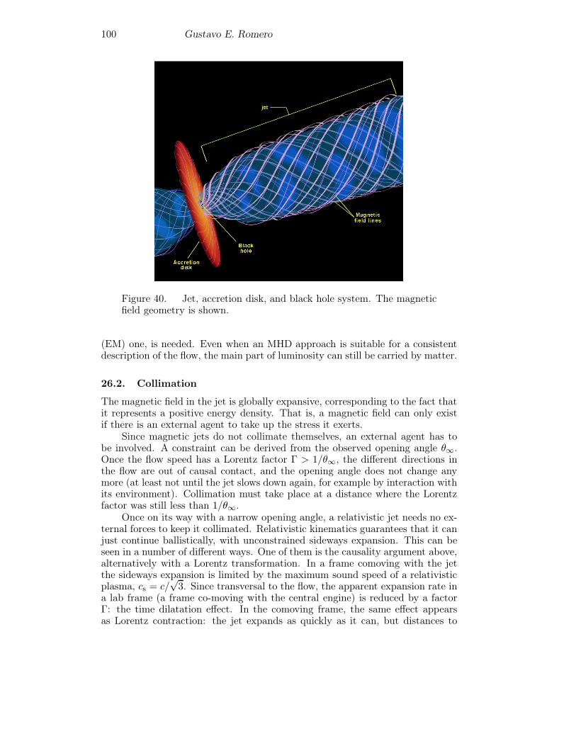
100 Gustavo E. Romero
Figure 40. Jet, accretion disk, and black hole system. The magneticfield geometry is shown.
(EM) one, is needed. Even when an MHD approach is suitable for a consistentdescription of the flow, the main part of luminosity can still be carried by matter.
26.2. Collimation
The magnetic field in the jet is globally expansive, corresponding to the fact thatit represents a positive energy density. That is, a magnetic field can only existif there is an external agent to take up the stress it exerts.
Since magnetic jets do not collimate themselves, an external agent has tobe involved. A constraint can be derived from the observed opening angle θ∞.Once the flow speed has a Lorentz factor Γ > 1/θ∞, the different directions inthe flow are out of causal contact, and the opening angle does not change anymore (at least not until the jet slows down again, for example by interaction withits environment). Collimation must take place at a distance where the Lorentzfactor was still less than 1/θ∞.
Once on its way with a narrow opening angle, a relativistic jet needs no ex-ternal forces to keep it collimated. Relativistic kinematics guarantees that it canjust continue ballistically, with unconstrained sideways expansion. This can beseen in a number of different ways. One of them is the causality argument above,alternatively with a Lorentz transformation. In a frame comoving with the jetthe sideways expansion is limited by the maximum sound speed of a relativisticplasma, cs = c/
√3. Since transversal to the flow, the apparent expansion rate in
a lab frame (a frame co-moving with the central engine) is reduced by a factorΓ: the time dilatation effect. In the comoving frame, the same effect appearsas Lorentz contraction: the jet expands as quickly as it can, but distances to
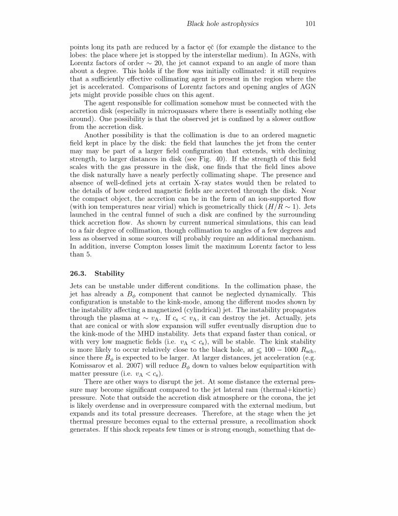
Black hole astrophysics 101
points long its path are reduced by a factor ęč (for example the distance to thelobes: the place where jet is stopped by the interstellar medium). In AGNs, withLorentz factors of order ∼ 20, the jet cannot expand to an angle of more thanabout a degree. This holds if the flow was initially collimated: it still requiresthat a sufficiently effective collimating agent is present in the region where thejet is accelerated. Comparisons of Lorentz factors and opening angles of AGNjets might provide possible clues on this agent.
The agent responsible for collimation somehow must be connected with theaccretion disk (especially in microquasars where there is essentially nothing elsearound). One possibility is that the observed jet is confined by a slower outflowfrom the accretion disk.
Another possibility is that the collimation is due to an ordered magneticfield kept in place by the disk: the field that launches the jet from the centermay may be part of a larger field configuration that extends, with decliningstrength, to larger distances in disk (see Fig. 40). If the strength of this fieldscales with the gas pressure in the disk, one finds that the field lines abovethe disk naturally have a nearly perfectly collimating shape. The presence andabsence of well-defined jets at certain X-ray states would then be related tothe details of how ordered magnetic fields are accreted through the disk. Nearthe compact object, the accretion can be in the form of an ion-supported flow(with ion temperatures near virial) which is geometrically thick (H/R ∼ 1). Jetslaunched in the central funnel of such a disk are confined by the surroundingthick accretion flow. As shown by current numerical simulations, this can leadto a fair degree of collimation, though collimation to angles of a few degrees andless as observed in some sources will probably require an additional mechanism.In addition, inverse Compton losses limit the maximum Lorentz factor to lessthan 5.
26.3. Stability
Jets can be unstable under different conditions. In the collimation phase, thejet has already a Bφ component that cannot be neglected dynamically. Thisconfiguration is unstable to the kink-mode, among the different modes shown bythe instability affecting a magnetized (cylindrical) jet. The instability propagatesthrough the plasma at ∼ vA. If cs < vA, it can destroy the jet. Actually, jetsthat are conical or with slow expansion will suffer eventually disruption due tothe kink-mode of the MHD instability. Jets that expand faster than conical, orwith very low magnetic fields (i.e. vA < cs), will be stable. The kink stabilityis more likely to occur relatively close to the black hole, at ∼< 100 − 1000 Rsch,since there Bφ is expected to be larger. At larger distances, jet acceleration (e.g.Komissarov et al. 2007) will reduce Bφ down to values below equipartition withmatter pressure (i.e. vA < cs).
There are other ways to disrupt the jet. At some distance the external pres-sure may become significant compared to the jet lateral ram (thermal+kinetic)pressure. Note that outside the accretion disk atmosphere or the corona, the jetis likely overdense and in overpressure compared with the external medium, butexpands and its total pressure decreases. Therefore, at the stage when the jetthermal pressure becomes equal to the external pressure, a recollimation shockgenerates. If this shock repeats few times or is strong enough, something that de-
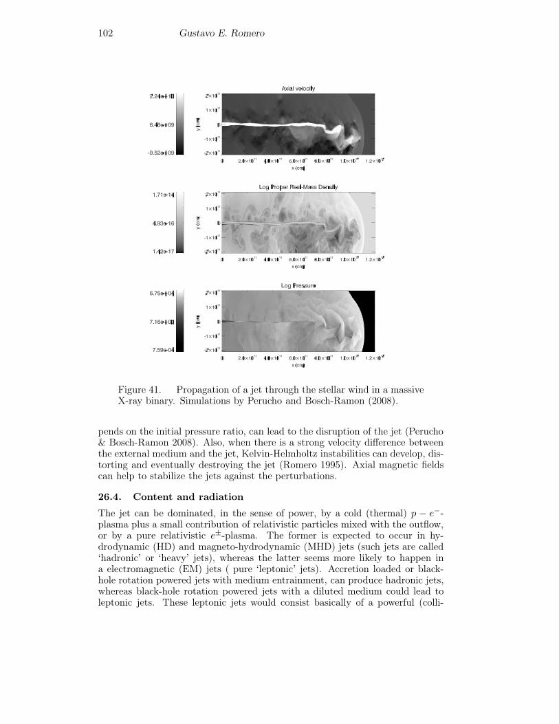
102 Gustavo E. Romero
Figure 41. Propagation of a jet through the stellar wind in a massiveX-ray binary. Simulations by Perucho and Bosch-Ramon (2008).
pends on the initial pressure ratio, can lead to the disruption of the jet (Perucho& Bosch-Ramon 2008). Also, when there is a strong velocity difference betweenthe external medium and the jet, Kelvin-Helmholtz instabilities can develop, dis-torting and eventually destroying the jet (Romero 1995). Axial magnetic fieldscan help to stabilize the jets against the perturbations.
26.4. Content and radiation
The jet can be dominated, in the sense of power, by a cold (thermal) p − e−-plasma plus a small contribution of relativistic particles mixed with the outflow,or by a pure relativistic e±-plasma. The former is expected to occur in hy-drodynamic (HD) and magneto-hydrodynamic (MHD) jets (such jets are called‘hadronic’ or ‘heavy’ jets), whereas the latter seems more likely to happen ina electromagnetic (EM) jets ( pure ‘leptonic’ jets). Accretion loaded or black-hole rotation powered jets with medium entrainment, can produce hadronic jets,whereas black-hole rotation powered jets with a diluted medium could lead toleptonic jets. These leptonic jets would consist basically of a powerful (colli-

Black hole astrophysics 103
mated) electromagnetic wave carrying just some e± injected by pair creation atthe base of the jet.
In HD and low magnetization MHD jets, the particle kinetic energy associ-ated with the motion in the jet direction (i.e. the bulk motion; eb = (Γj−1)mc2)is expected to be much larger than the energy associated with jet expansion (i.e.eexp ≈ mv2exp/2) and temperature (i.e. ekT = k T ). This implies strong collima-tion, and a low sound (cs) or Alfven speed (vA) in the jet plasma compared tothe jet velocity, i.e. the jet will be strongly supersonic/superalfvenic. If this werenot the case, the jet could still be collimated by external pressure, but would bedifficult to keep it collimated on long distances. For jets with dynamics dom-inated by the EM fields the temperature of the plasma could be very large aslong as collimation is satisfied, i.e. the external and magnetic pressure shouldbe well above the thermal pressure. Otherwise, the flow would be uncollimated.The realization of the different situations may take place in each jet at differ-ent stages of their evolution. The jet could be EM/leptonic at its very base,MHD/hadronic through external medium entrainment at intermediate scales,and HD at the largest scales after magnetic energy has gone to accelerate thejet.
As long as jets are radiatively efficient, they will shine across the EM spec-trum and could be detected, but when the conditions in the plasma are notsuitable for the production of significant radiation, they may keep dark all theway to their termination regions. The radiation from jets can be thermal (contin-uum and lines), although the detection of thermal jets is rare since the requireddensities are high, and T and vj moderate. The detection of non-thermal ra-diation from jets, mainly in the radio band, is more common. For that, it isrequired that some particles will be accelerated up to relativistic energies, wellabove k T , and at least the presence of magnetic field, since these are the in-gredients of synchrotron emission. Efficient high-energy and very high-energyemission is possible if the radiation and/or the matter fields are dense enough.This radiation can be produced by inverse Compton scattering, when acceleratedleptons are present, or by proton-proton collisions, when accelerated hadrons arepresent (e.g. Bosch-Ramon et al. 2006; Romero et al. 2003). For a compre-hensive description, including particle transport, see Vila & Romero (2010) andReynoso et al. (2010).
27. Evidence for black holes in the universe
28. White holes and gravastars
The analytical extension of the Schwarzschild solution in Kruskal-Szekeres coor-dinates shows a region that is singular and covered by an horizon but from wheregeodesic lines emerge. Such an extension can be interpreted as a time-reversalimage of a black hole: the matter from an expanding cloud began to expand fromthe horizon. Such space-time regions are known as white holes (Novikov 1964,Ne’eman 1965). White holes cannot result from the collapse of physical objectsin the real Universe, but they could be imagined to be intrinsic features of space-time. A white hole acts as a source that ejects matter from its event horizon.The sign of the acceleration is invariant under time reversal, so both black and
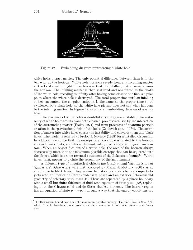
104 Gustavo E. Romero
Figure 42. Embedding diagram representing a white hole.
white holes attract matter. The only potential difference between them is in thebehavior at the horizon. White hole horizons recede from any incoming matterat the local speed of light, in such a way that the infalling matter never crossesthe horizon. The infalling matter is then scattered and re-emitted at the deathof the white hole, receding to infinity after having come close to the final singularpoint where the white hole is destroyed. The total proper time until an infallingobject encounters the singular endpoint is the same as the proper time to beswallowed by a black hole, so the white hole picture does not say what happensto the infalling matter. In Figure 42 we show an embedding diagram of a whitehole.
The existence of white holes is doubtful since they are unstable. The insta-bility of white holes results from both classical processes caused by the interactionof the surrounding matter (Frolov 1974) and from processes of quantum particlecreation in the gravitational field of the holes (Zeldovich et al. 1974). The accre-tion of matter into white holes causes the instability and converts them into blackholes. The reader is referred to Frolov & Novikov (1998) for a detailed discussion.In addition, we notice that the entropy of a black hole is related to the horizonarea in Planck units, and this is the most entropy which a given region can con-tain. When an object flies out of a white hole, the area of the horizon alwaysdecreases by more than the maximum possible entropy that can be squeezed intothe object, which is a time-reversed statement of the Bekenstein bound17. Whiteholes, then, appear to violate the second law of thermodynamics.
A different type of hypothetical objects are Gravitational Vacuum Stars or“gravastars”. Gravastars were first proposed by Mazur & Mottola (2001) as analternative to black holes. They are mathematically constructed as compact ob-jects with an interior de Sitter condensate phase and an exterior Schwarzschildgeometry of arbitrary total mass M . These are separated by a phase boundarywith a small but finite thickness of fluid with equation of state p = +ρc2, replac-ing both the Schwarzschild and de Sitter classical horizons. The interior regionhas an equation of state p = −ρc2, in such a way that the energy conditions are
17The Bekenstein bound says that the maximum possible entropy of a black hole is S = A/4,where A is the two-dimensional area of the black hole’s event horizon in units of the Planckarea.
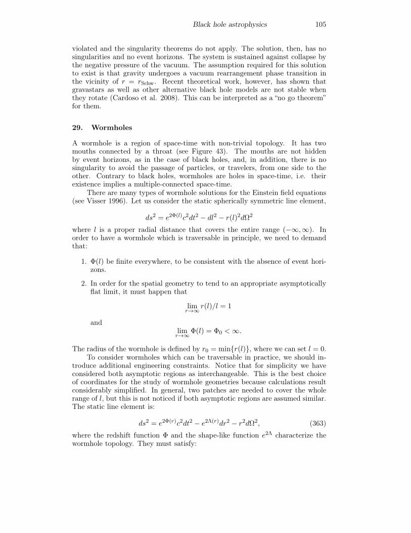
Black hole astrophysics 105
violated and the singularity theorems do not apply. The solution, then, has nosingularities and no event horizons. The system is sustained against collapse bythe negative pressure of the vacuum. The assumption required for this solutionto exist is that gravity undergoes a vacuum rearrangement phase transition inthe vicinity of r = rSchw. Recent theoretical work, however, has shown thatgravastars as well as other alternative black hole models are not stable whenthey rotate (Cardoso et al. 2008). This can be interpreted as a “no go theorem”for them.
29. Wormholes
A wormhole is a region of space-time with non-trivial topology. It has twomouths connected by a throat (see Figure 43). The mouths are not hiddenby event horizons, as in the case of black holes, and, in addition, there is nosingularity to avoid the passage of particles, or travelers, from one side to theother. Contrary to black holes, wormholes are holes in space-time, i.e. theirexistence implies a multiple-connected space-time.
There are many types of wormhole solutions for the Einstein field equations(see Visser 1996). Let us consider the static spherically symmetric line element,
ds2 = e2Φ(l)c2dt2 − dl2 − r(l)2dΩ2
where l is a proper radial distance that covers the entire range (−∞,∞). Inorder to have a wormhole which is traversable in principle, we need to demandthat:
1. Φ(l) be finite everywhere, to be consistent with the absence of event hori-zons.
2. In order for the spatial geometry to tend to an appropriate asymptoticallyflat limit, it must happen that
limr→∞ r(l)/l = 1
andlimr→∞Φ(l) = Φ0 <∞.
The radius of the wormhole is defined by r0 = min{r(l)}, where we can set l = 0.To consider wormholes which can be traversable in practice, we should in-
troduce additional engineering constraints. Notice that for simplicity we haveconsidered both asymptotic regions as interchangeable. This is the best choiceof coordinates for the study of wormhole geometries because calculations resultconsiderably simplified. In general, two patches are needed to cover the wholerange of l, but this is not noticed if both asymptotic regions are assumed similar.The static line element is:
ds2 = e2Φ(r)c2dt2 − e2Λ(r)dr2 − r2dΩ2, (363)
where the redshift function Φ and the shape-like function e2Λ characterize thewormhole topology. They must satisfy:
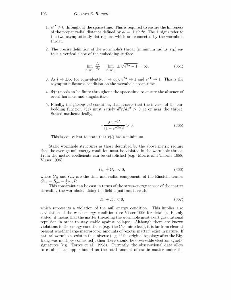
106 Gustavo E. Romero
1. e2Λ ≥ 0 throughout the space-time. This is required to ensure the finitenessof the proper radial distance defined by dl = ± eΛ dr. The ± signs refer tothe two asymptotically flat regions which are connected by the wormholethroat.
2. The precise definition of the wormhole’s throat (minimum radius, rth) en-tails a vertical slope of the embedding surface
limr→r+
th
dz
dr= lim
r→r+th
±√e2Λ − 1 = ∞. (364)
3. As l → ±∞ (or equivalently, r → ∞), e2Λ → 1 and e2Φ → 1. This is theasymptotic flatness condition on the wormhole space-time.
4. Φ(r) needs to be finite throughout the space-time to ensure the absence ofevent horizons and singularities.
5. Finally, the flaring out condition, that asserts that the inverse of the em-bedding function r(z) must satisfy d2r/dz2 > 0 at or near the throat.Stated mathematically,
− Λ′ e−2Λ
(1− e−2Λ)2> 0. (365)
This is equivalent to state that r(l) has a minimum.
Static wormhole structures as those described by the above metric requirethat the average null energy condition must be violated in the wormhole throat.From the metric coefficients can be established (e.g. Morris and Thorne 1988,Visser 1996):
Gtt +Grr < 0, (366)
where Gtt and Grr are the time and radial components of the Einstein tensor:Gμν = Rμν − 1
2gμνR.This constraint can be cast in terms of the stress-energy tensor of the matter
threading the wormhole. Using the field equations, it reads
Ttt + Trr < 0, (367)
which represents a violation of the null energy condition. This implies alsoa violation of the weak energy condition (see Visser 1996 for details). Plainlystated, it means that the matter threading the wormhole must exert gravitationalrepulsion in order to stay stable against collapse. Although there are knownviolations to the energy conditions (e.g. the Casimir effect), it is far from clear atpresent whether large macroscopic amounts of “exotic matter” exist in nature. Ifnatural wormholes exist in the universe (e.g. if the original topology after the Big-Bang was multiply connected), then there should be observable electromagneticsignatures (e.g. Torres et al. 1998). Currently, the observational data allowto establish an upper bound on the total amount of exotic matter under the
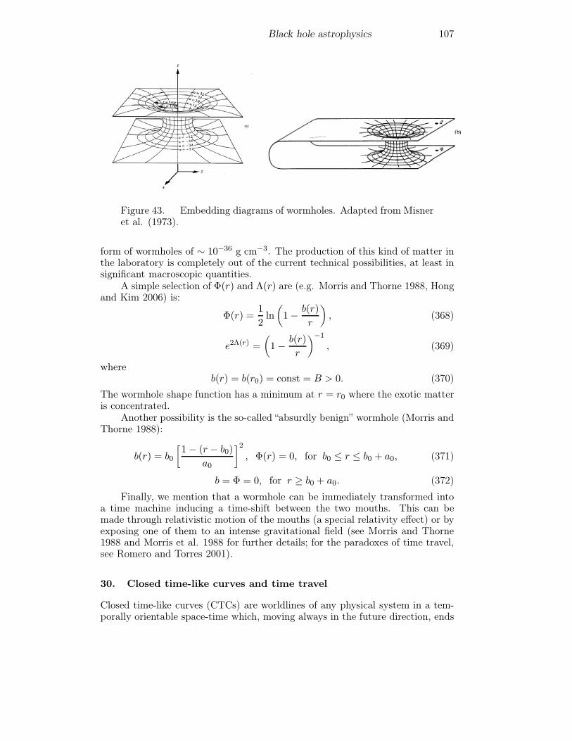
Black hole astrophysics 107
Figure 43. Embedding diagrams of wormholes. Adapted from Misneret al. (1973).
form of wormholes of ∼ 10−36 g cm−3. The production of this kind of matter inthe laboratory is completely out of the current technical possibilities, at least insignificant macroscopic quantities.
A simple selection of Φ(r) and Λ(r) are (e.g. Morris and Thorne 1988, Hongand Kim 2006) is:
Φ(r) =1
2ln
(1− b(r)
r
), (368)
e2Λ(r) =
(1− b(r)
r
)−1
, (369)
whereb(r) = b(r0) = const = B > 0. (370)
The wormhole shape function has a minimum at r = r0 where the exotic matteris concentrated.
Another possibility is the so-called “absurdly benign” wormhole (Morris andThorne 1988):
b(r) = b0
[1− (r − b0)
a0
]2, Φ(r) = 0, for b0 ≤ r ≤ b0 + a0, (371)
b = Φ = 0, for r ≥ b0 + a0. (372)
Finally, we mention that a wormhole can be immediately transformed intoa time machine inducing a time-shift between the two mouths. This can bemade through relativistic motion of the mouths (a special relativity effect) or byexposing one of them to an intense gravitational field (see Morris and Thorne1988 and Morris et al. 1988 for further details; for the paradoxes of time travel,see Romero and Torres 2001).
30. Closed time-like curves and time travel
Closed time-like curves (CTCs) are worldlines of any physical system in a tem-porally orientable space-time which, moving always in the future direction, ends
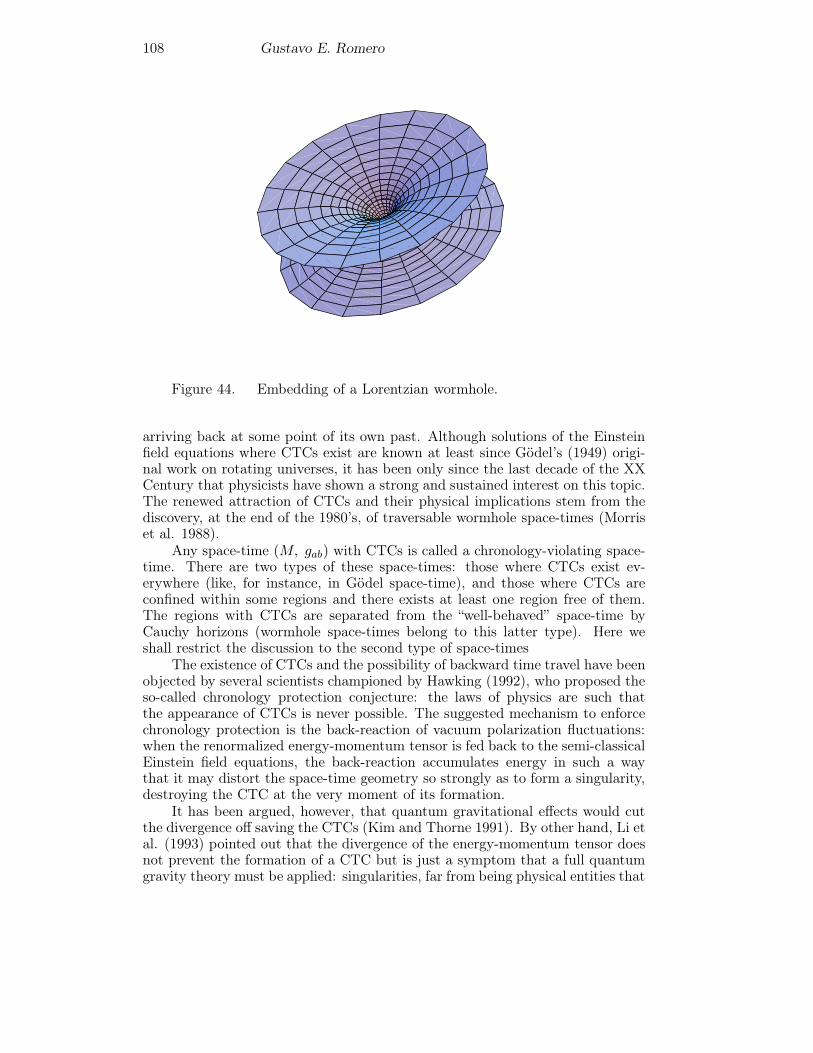
108 Gustavo E. Romero
Figure 44. Embedding of a Lorentzian wormhole.
arriving back at some point of its own past. Although solutions of the Einsteinfield equations where CTCs exist are known at least since Gödel’s (1949) origi-nal work on rotating universes, it has been only since the last decade of the XXCentury that physicists have shown a strong and sustained interest on this topic.The renewed attraction of CTCs and their physical implications stem from thediscovery, at the end of the 1980’s, of traversable wormhole space-times (Morriset al. 1988).
Any space-time (M, gab) with CTCs is called a chronology-violating space-time. There are two types of these space-times: those where CTCs exist ev-erywhere (like, for instance, in Gödel space-time), and those where CTCs areconfined within some regions and there exists at least one region free of them.The regions with CTCs are separated from the “well-behaved” space-time byCauchy horizons (wormhole space-times belong to this latter type). Here weshall restrict the discussion to the second type of space-times
The existence of CTCs and the possibility of backward time travel have beenobjected by several scientists championed by Hawking (1992), who proposed theso-called chronology protection conjecture: the laws of physics are such thatthe appearance of CTCs is never possible. The suggested mechanism to enforcechronology protection is the back-reaction of vacuum polarization fluctuations:when the renormalized energy-momentum tensor is fed back to the semi-classicalEinstein field equations, the back-reaction accumulates energy in such a waythat it may distort the space-time geometry so strongly as to form a singularity,destroying the CTC at the very moment of its formation.
It has been argued, however, that quantum gravitational effects would cutthe divergence off saving the CTCs (Kim and Thorne 1991). By other hand, Li etal. (1993) pointed out that the divergence of the energy-momentum tensor doesnot prevent the formation of a CTC but is just a symptom that a full quantumgravity theory must be applied: singularities, far from being physical entities that
Black hole astrophysics 109
can act upon surrounding objects, are manifestations of the breakdown of thegravitational theory. In any case, we cannot draw definitive conclusions with thesemi-classical tools at our disposal (see Earman 1995 for additional discussion).
But even if the energy-momentum tensor of vacuum polarization diverges atthe Cauchy horizon it is not necessarily implied that CTCs must be destroyed,since the equations can be well-behaved in the region inside the horizon (Li et al.1993). In particular, wormhole space-times could be stabilized against vacuumfluctuations introducing reflecting boundaries between the wormhole mouths (Li1994) or using several wormholes to create CTCs (Thorne 1992, Visser 1997).
Even Hawking has finally recognized that back-reaction does not necessarilyenforce chronology protection (Cassidy and Hawking 1998). Although the questfor finding an effective mechanism to avoid CTCs continues, it is probable thatthe definitive solution to the problem should wait until a complete theory ofquantum gravity can be formulated. In the meantime, the profound physicalconsequences of time travel in General Relativity should be explored in order topush this theory to its ultimate limits, to the region where the very foundationsof the theory must be revisited.
A different kind of objection to CTC formation is that they allow illogicalsituations like the “grandfather” paradox18 which would be expressing that thecorresponding solutions of the field equations are “non-physical”. This is a com-mon place and has been conveniently refuted by Earman (1995), among others(see also Nahin 1999 and references therein). Grandfather-like paradoxes do notimply illogical situations. In particular, they do not mean that local determinismdoes not operate in chronology-violating space-times because it is always possibleto choose a neighborhood of any point of the manifold such that the equationsthat represent the laws of physics have appropriate solutions. Past cannot bechanged (the space-time manifold is unique) but it can be causally affected fromthe future, according to General Relativity. The grandfather paradox, as pointedout by Earman 1995, is just a manifestation of the fact consistency constraintsmust exist between the local and the global order of affairs in space-time. Thisleads directly to the so-called Principle of Self-Consistency (PSC).
30.1. The Principle of Self-Consistency
In space-times with CTCs, past and future are no longer globally distinct. Eventson CTCs should causally influence each other along a time-loop in a self-adjusted,consistent way in order to occur in the real universe. This has been stated byFriedman et al. (1990) as a general principle of physics:
Principle of Self-Consistency: The only solutions to the laws of physics thatoccur locally in the real universe are those which are globally self-consistent.
When applied to the grandfather paradox, the PSC says that the grandfa-ther cannot be killed (a local action) because in the far future this would generatean inconsistency with the global world line of the time traveler. Just consistenthistories can develop in the universe. An alternative way to formulate the PSC
18The grandfather paradox: A time traveler goes to his past and kills his young grandfather thenavoiding his own birth and, consequently, the time travel in which he killed his grandfather.
110 Gustavo E. Romero
is to state that (Earman 1995):
The laws of physics are such that any local solution of their equations thatrepresents a feature of the real universe must be extensible to a global solution.
The principle is not tautological or merely prescriptive, since it is clear thatlocal observations can provide information of the global structure of the world:it is stated that there is a global-to-local order in the universe in such a waythat certain local actions are ruled out by the global properties of the space-timemanifold.
If the PSC is neither a tautological statement nor a methodological rule,what is then its epistemological status? It has been suggested that it could be abasic law of physics –in the same sense that the Einstein field equations are lawsof physics– (Earman 1995). This would imply that there is some “new physics"behind the PSC. By other hand, Carlini et al. (1995) have proposed, on the basisof some simple examples, that the PSC could be a consequence of the Principleof Minimal Action. In this case, no new physics would be involved. Contrary tothese opinions, that see in the PSC a law statement, or at least a consequenceof law statements, we suggest that this principle actually is a metanomologicalstatement, like the Principle of General Covariance among others (see Bunge1961 for a detailed discussion of metanomological statements). This means thatthe reference class of the PSC is not formed by physical systems, but by laws ofphysical systems. The usual laws are restrictions to the state space of physicalsystems. Metanomological statements are laws of laws, i.e. restrictions on theglobal network of laws that thread the universe. The requirement of consistencyconstraints would then be pointing out the existence of deeper level super-laws,which enforce the harmony between local and global affairs in space-time. Justin this sense it is fair to say that “new physics" is implied.
30.2. Causal loops: Self-existent objects
Although the PSC eliminates grandfather-like paradoxes from chronology-violatingspace-times, other highly perplexing situations remain. The most obscure ofthese situations is the possibility of an ontology with self-existent objects. Letus illustrate with an example what we understand by such an object:
Suppose that, in a space-time where CTCs exist, a time traveler takes a rideon a time machine carrying a book with her. She goes back to the past, forgetsthe book in -what will be- her laboratory, and returns to the future. The bookremains then hidden until the time traveler finds it just before starting her timetrip, carrying the book with her.
It is not hard to see that the primordial origin of the book remains a mystery.Where does the book come from?. This puzzle has been previously mentionedin philosophical literature by Nerlich (1981) and MacBeath (1982). Physicists,instead, have not paid much attention to it, despite the interesting fact thatthe described situation is apparently not excluded by the PSC: the local andglobal structures of the loop are perfectly harmonious and there is no causalityviolations. There is just a book never created, never printed, but, somehow,
Black hole astrophysics 111
existing in space-time. It has been suggested (Nerlich 1981) that if CTCs exist,then we are committed to accept an ontology of self-existing objects: they arejust out there, trapped in space-time. There is no sense in asking where they arefrom. Even energy is conserved if we admit that the system to be considered is notonly the present time-slice of the manifold but rather the two slices connected bythe time loop: the energy removed from the present time (Mbookc
2) is depositedin the past.
However, that the acceptance of such a bizarre ontology proceeds from anincorrect application of the PSC. This principle is always discussed within thecontext of General Relativity, although actually it should encompass all physicallaws. A fully correct formulation of the PSC should read laws of nature where inthe formulation given above it is said laws of physics. What should be demandedis total consistency and not only consistency in the solutions of the Einsteinfield equations. In particular, when thermodynamics is included in the analysis,the loop of a self-existing objects becomes inconsistent because, due to entropicdegradation, the final and initial states of the object do not match (Romero &Torres 2001). Moreover, even more strange paradoxes, related to human self-reproduction like the amazing Jocasta paradox (Harrison 1979), can be provento be non-consistent when the laws of genetics are taken into account (see Nahin1999 and references therein).
30.3. Information loops and the PSC
Consider the local light cone of a time traveler. There are three, and only three,possible final destinations for a backwards time trip. The arrival point could bea within the past light cone, b on the edge of it, or c elsewhere out of the cone.In the case a the time traveler can transmit information at a velocity v ≤ c andaffect its own past. Information transmitted in case b that propagates at thevelocity of light, instead, will arrive at the very moment when the time travelstarted. In case c, the information flux can only reach the future of the timetraveler. However, even in the last case, if more than one time machine areavailable (for instance as in the situation known as a Roman ring, where thereare two wormholes in relative motion) the past might be affected by informationflux from the future. The conclusion, then, is that whatever the final destiny ofthe time-traveler is, in principle, she could always affect her own past. Otherwisestated, chronology-violating space-times generally admit information loops: theycannot be excluded on the only basis of the PSC.
Although the PSC does not preclude that within chronology-violating re-gions information steaming from the future can affect the past, it at least imposesconstraints on the way this can be done. In fact, any physical process causallytriggered by the backwards information flux must be consistent with the pasthistory of the universe. This means that if a time traveler goes back to his pastand tries, for instance, to communicate the contents of the theory of specialrelativity to the scientific community before 1905, she will fail because at herdeparture it was historically clear that the first paper on special relativity waspublished by Albert Einstein in June 1905. The details of her failure will dependon the details of her travel and attempt, in the same way that the details ofthe failure of a perpetual motion machine depends on the approach used by theimprudent inventor. All we can say a priori is that the laws of physics are such
112 Gustavo E. Romero
that these attempts cannot succeed and information cannot propagate arbitrar-ily in space-time. It is precisely due to the PSC that we know that our past isnot significantly affected from the future: we know that till now, knowledge hasbeen generated by evolutionary processes, i.e. there is small room in history forinformation loops. This does not necessarily mean that the same is valid for theentire space-time.
31. The future of black holes
According to Eq. (255), an isolated black hole with M = 10 M� would have alifetime of more than 1066 yr. This is 56 orders of magnitude longer than the ageof the universe19. However, if the mass of the black hole is small, then it couldevaporate within the Hubble time. A primordial black hole, created by extremelyenergetic collisions short after the Big Bang, should have a mass of at least 1015g in order to exist today. Less massive black holes must have already evaporated.What happens when a black hole losses its mass so it cannot sustain an eventhorizon anymore?. As the black hole evaporates, its temperature raises. Whenit is cold, it radiates low energy photons. When the temperature increases, moreand more energetic particles will be emitted. At some point gamma rays wouldbe produced. If there is a population of primordial black holes, their radiationshould contribute to the diffuse gamma-ray background. This background seemsto be dominated by the contribution of unresolved Active Galactic Nuclei andcurrent observations indicate that if there were primordial black holes their massdensity should be less than 10−8 Ω, where Ω is the cosmological density param-eter (∼ 1). After producing gamma rays, the mini black hole would produceleptons, quarks, and super-symmetric particles, if they exist. At the end theblack hole would have a quantum size and the final remnant will depend on thedetails of how gravity behaves at Planck scales. The final product might be astable, microscopic object with a mass close to the Planck mass. Such particlesmight contribute to the dark matter present in the Galaxy and in other galaxiesand clusters. The cross-section of black hole relics is extremely small: 10−66
cm2 (Frolov and Novikov 1998), hence they would be basically non-interactingparticles.
A different possibility, advocated by Hawking (1976), is that, as a result ofthe evaporation nothing is left behind: all the energy is radiated. This createsa puzzle about the fate of the information stored in the black hole: is it radi-ated away during the black hole lifetime or does it simply disappear from theuniverse?.
Actually, the very question is likely meaningless: information is not a prop-erty of physical systems. Information is a property of languages, and languagesare human constructs. The physical property usually confused with informationis entropy. The reason is that a same mathematical formalism can be used todescribe both properties. Of course, this does not mean that these quite differ-ent properties are identical. Black holes, as we have seen, have huge entropy. Is
19We assume that the universe originated at the Big Bang, although, of course, this needs notto be necessarily the case.
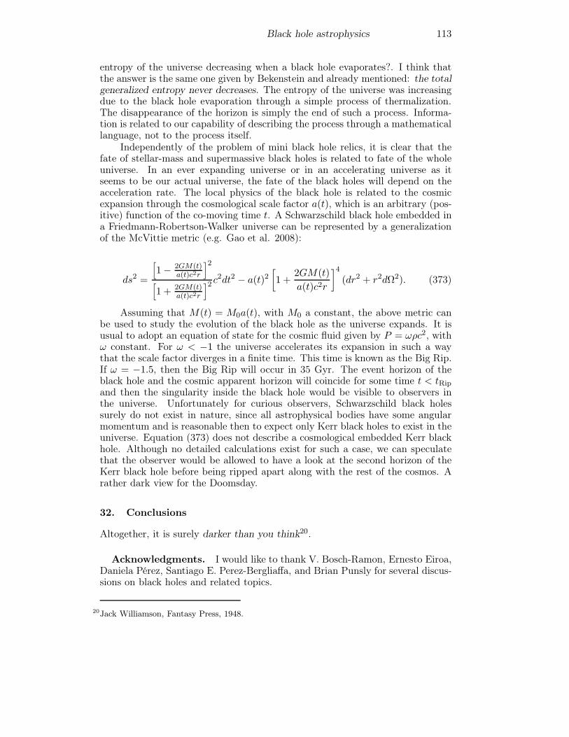
Black hole astrophysics 113
entropy of the universe decreasing when a black hole evaporates?. I think thatthe answer is the same one given by Bekenstein and already mentioned: the totalgeneralized entropy never decreases. The entropy of the universe was increasingdue to the black hole evaporation through a simple process of thermalization.The disappearance of the horizon is simply the end of such a process. Informa-tion is related to our capability of describing the process through a mathematicallanguage, not to the process itself.
Independently of the problem of mini black hole relics, it is clear that thefate of stellar-mass and supermassive black holes is related to fate of the wholeuniverse. In an ever expanding universe or in an accelerating universe as itseems to be our actual universe, the fate of the black holes will depend on theacceleration rate. The local physics of the black hole is related to the cosmicexpansion through the cosmological scale factor a(t), which is an arbitrary (pos-itive) function of the co-moving time t. A Schwarzschild black hole embedded ina Friedmann-Robertson-Walker universe can be represented by a generalizationof the McVittie metric (e.g. Gao et al. 2008):
ds2 =
[1− 2GM(t)
a(t)c2r
]2[1 + 2GM(t)
a(t)c2r
]2 c2dt2 − a(t)2[1 +
2GM(t)
a(t)c2r
]4(dr2 + r2dΩ2). (373)
Assuming that M(t) = M0a(t), with M0 a constant, the above metric canbe used to study the evolution of the black hole as the universe expands. It isusual to adopt an equation of state for the cosmic fluid given by P = ωρc2, withω constant. For ω < −1 the universe accelerates its expansion in such a waythat the scale factor diverges in a finite time. This time is known as the Big Rip.If ω = −1.5, then the Big Rip will occur in 35 Gyr. The event horizon of theblack hole and the cosmic apparent horizon will coincide for some time t < tRip
and then the singularity inside the black hole would be visible to observers inthe universe. Unfortunately for curious observers, Schwarzschild black holessurely do not exist in nature, since all astrophysical bodies have some angularmomentum and is reasonable then to expect only Kerr black holes to exist in theuniverse. Equation (373) does not describe a cosmological embedded Kerr blackhole. Although no detailed calculations exist for such a case, we can speculatethat the observer would be allowed to have a look at the second horizon of theKerr black hole before being ripped apart along with the rest of the cosmos. Arather dark view for the Doomsday.
32. Conclusions
Altogether, it is surely darker than you think20.
Acknowledgments. I would like to thank V. Bosch-Ramon, Ernesto Eiroa,Daniela Pérez, Santiago E. Perez-Bergliaffa, and Brian Punsly for several discus-sions on black holes and related topics.
20Jack Williamson, Fantasy Press, 1948.
114 Gustavo E. Romero
Appendix A.1. Manifolds and topology
Appendix A.2. General definition of space-time
Appendix A.3. The anisotropy of time
The electromagnetic radiation can be described in the terms of the 4-potentialAμ, which in the Lorentz gauge satisfies:
∂ν∂νAμ(�r, t) = 4πjμ(�r, t), (374)
with c = 1 and jμ the 4-current. With appropriate boundary conditions ispossible to write Aμ as a functional of the sources jμ. The retarded and advancedsolutions are:
Aμret(�r, t) =
∫ jμ(�r, t−
∣∣∣�r − �r′∣∣∣)∣∣∣�r − �r′
∣∣∣ d3�r′, (375)
Aμadv(�r, t) =
∫ jμ(�r, t+
∣∣∣�r − �r′∣∣∣)∣∣∣�r − �r′
∣∣∣ d3�r′. (376)
The two functionals of jμ(�r, t) are related to one another by a time reversaltransformation. The solution (375) is contributed by all sources in the causalpast of the space-time point (�r, t) and the solution (375) by all the sources inthe causal future of that point. The linear combinations of these solutions arealso solutions, since the equations are linear and the Principle of Superpositionholds. It is usual to consider only the retarded potential as physical meaningfulin order to estimate the electromagnetic field at (�r, t): Fμν
ret = ∂μAνret − ∂νAμ
ret.However, there seems to be no compelling reason for such a choice. We canadopt, for instance, (in what follows we use a simplified notation and boundaryconditions such as the surface contribution is zero):
Aμ(�r, t) =1
2
∫V(adv + ret) dV. (377)
If the space-time is curve (R �= 0), the null cones that determines the localcausal structure will not be symmetric around the point p (�r, t). Then,
Lμ = limV→∞
[∫Vret−
∫Vadv
]dV �= 0. (378)
If gμνLμT ν �= 0, with T ν = (1, 0, 0, 0) there is a preferred direction for flow ofthe Poynting flux in space-time. In a black hole interior this direction is towardsthe singularity. In an expanding Universe, it is in the global future direction.We see, then, that time, in a general space-time (M,gab), is anisotropic. Thereis a global to local relation given by the Poynting flux as determined by the cur-vature of space-time that indicates the direction in which events occur. Physicalprocesses, inside a black hole, have a different orientation that outside, and thecausal structure of the world is determined by the dynamics of space-time and
Black hole astrophysics 115
the initial conditions. Macroscopic irreversibility21 and time anisotropy emergefrom essentially reversible laws. For additional details see Romero (2010).
Appendix A.4. The ontology of the world
The ontology is the part of metaphysics that deals with the most general featuresof the world. It essentially provides theories about the structure and basic con-tents of the world. These theories are presupposed by physical theories, which areconcerned with the detailed laws and specific characteristics of whatever exists.
The concept of individual is the basic primitive concept of any ontologicaltheory. Individuals associate themselves with other individuals to yield newindividuals. It follows that they satisfy a calculus, and that they are rigorouslycharacterized only through the laws of such calculus. These laws are set with theaim of reproducing the way real things associate. Specifically, it is postulatedthat every individual is an element of a set S in such a way that the structureS =< S, ◦,� > is a commutative monoid of idempotents. In the structure S, Sis to be interpreted as the set of all the individuals, the element � ∈ S as thenull individual, and the binary operation ◦ as the association of individuals. Itis easy to see that there are two classes of individuals: simple and composed.
D1 x ∈ S is composed ⇔ ∃ y, z ∈ S/x = y ◦ z.D2 x ∈ S is simple ⇔¬ ∃ y, z ∈ S/x = y ◦ z.D3 x � y ⇔ x ◦ y = y ( x is part of y ⇔ x ◦ y = y).
D4 C(x) ≡ {y ∈ S/y � x} (composition of x).
Real things differentiate from abstract individuals because they have a num-ber of properties in addition to their capability of association. These propertiescan be intrinsic (Pi) or relational (Pr). The intrinsic properties are inherentand they are represented by predicates or unary applications, while relationalproperties are represented by n-ary predicates, with n>1, as long as nonconcep-tual arguments are considered. For instance, the position and the velocity of aparticle are relational properties, but its charge is an intrinsic property.
P is called a substantial property if and only if some individual x possessesP :
D5 P ∈ P ⇔ (∃x)(x ∈ S ∧ Px).Here P is the set of all the substantial properties. The set of the properties of agiven individual x is
D6 P (x) ≡ {P ∈ P/Px}.
21Notice that the electromagnetic flux is related with the macroscopic concept of temperaturethrough the Stefan-Boltzmann law: L = AσSBT
4, where σSB = 5.670400 × 10⁻⁸J s−1m−2K−4
is the StefanŰBoltzmann constant.
116 Gustavo E. Romero
If two individuals have exactly the same properties they are the same:∀ x, y ∈ S if P (x) = P (y) ⇒ x ≡ y. Two individuals are identical if theirintrinsic properties are the same: x id↔ y ( they can differ only in their relationalproperties).
A detailed account of the theory of properties is given in Bunge (1977). Weonly give here two useful definitions:
D7 P is an inherited property of x⇔ P ∈ P (x)∧ (∃y)(y ∈ C(x)∧ y �= x∧P ∈P (y)).
D8 P is an emergent property of x ⇔ P ∈ P (x) ∧ ( (∀ y)C(x)(y �= x ) ⇒ P /∈P (y) ).
According to these definitions, mass is an inherited property and viscosity is anemergent property of a classical fluid.
An individual with its properties make up a thing X:
D9 XDf=< x,P (x) >.
The laws of association of things follow from those of the individuals. Theassociation of all things is the Universe (σU ). It should not be confused with theset of all things; this is only an abstract entity and not a thing.
Given a thing X =< x,P (x) >, a conceptual object named model Xm ofthe thing X can be constructed by a nonempty set M and a finite sequence F ofmathematical functions over M , each of them formally representing a propertyof x:
D10 XmDf=< M,F >, where F =< F1, . . . ,Fn > /Fi : M → Vi, 1 ≤ i ≤ n, Vi
vector space ,Fi = Pi ∈ P (x).
It is said then that Xm represents X: Xm=X (Bunge 1977).The state of the thing X can be characterized as follows:
D11 Let X be a thing with model Xm =< M,F >, such that each componentof the function
F =< F1, . . . ,Fn >:M → V1 × . . .× Vn.
represents some P ∈ P (x). Then Fi (1 ≤ i ≤ n) is named i-th statefunction of X, F is the total state function of X, and the value of F forsome m ∈ M, F(m), represents the state of X at m in the representationXm.
If all the Vi, 1 ≤ i ≤ n, are vector spaces, F is the state vector of X in therepresentation Xm, and V = V1 × . . . × Vn is the state space of X in therepresentation Xm.
The concept of physical law can be introduced as follows:
D12 Let Xm =< X,F > be a model for X. Any restriction on the possiblevalues of the components of F and any relation between two or more ofthem is a physical law if and only if it belongs to a consistent theory of theX and has been satisfactorily confirmed by the experiment.
Black hole astrophysics 117
We say that a thing X acts on a thing Y if X modifies the path of Y in itsspace state (X � Y : X acts on Y ).
We say that two things X and Y are connected if at least one of them actson the other. We come at last to the definition of system:
D13 A system is a thing composed by at least two connected things.
In particular, a physical system is a system ruled by physical laws. A set of thingsis not a system, because a system is a physical entity and not a set. A systemmay posses emergent properties with respect to the component subsystems. Thecomposition of the system σ with respect to a class A of things is (at the instantt):
CA(σ, t) = {X ∈ A/X � σ}.D14 σA(σ, t) = {X ∈ A/X �∈ CA(σ, t) ∧ (∃Y )CA(σ,t) ∧ (X � Y ∨ Y �X) )} is the
A-environment of σ at t.
If σA(σ, t) = ∅ ⇒ σ is closed at the instant t. In any other case we say that it isopen.
A specific physical system will be characterized by making explicit its spaceof physical states. This is done in the axiomatic basis of the physical theory (e.g.Perez-Bergliaffa et al. 1993, 1996).
Appendix A.5. Annotated bibliography on black holes
References
Abramowicz, M.A., et al. 1996, A&A, 313, 334Araudo, A.T., Bosch-Ramon, V., and Romero, G.E. 2009, A&A, 503, 673Arcos, H.I., and Pereira, J.G. 2004, Int. J. Mod. Phys. D13, 2193Arkani-Hamed, N., Dimopoulos, S., and Dvali, G.R. 1998, Phys. Lett B., 429,
263Baade, W., and Zwicky, F. 1934, Phys. Rev., 45, 138Begelman M., and Meier D.L. 1982, ApJ, 253, 873Bekenstein, J.D. 1973, Phys. Rev. D7, 2333Blandford, R.D., and Znajek, R.L. 1977, MNRAS, 179, 433Blandford, R. D., and Payne, D. G. 1982, MNRAS, 199, 883Bondi, H., and Hoyle, F. 1944, MNRAS, 104, 203Bondi, H. 1952, MNRAS, 112, 195Born, M., and Infeld, L. 1934, Proc. R. Soc. London, A 144, 425Bosch-Ramon, V., Romero, and G E., Paredes, J. M. 2006, A&A, 447, 263Brans, C.H., and Dicke, R.H. 1961, Phys. Rev., 124, 925Brown, G.B., et al. 1999, Physics Reports, 333, 471Bunge, M. 1961, Am. J. Phys., 29, 518Bunge, M. 1977, Ontology I: The Furniture of the World, Kluwer, DordrechtCardoso, V., et al. 2008, Phys.Rev.D, 77, id. 124044
118 Gustavo E. Romero
Carlini, A., et al. 1995, Int. J. Mod. Phys. D, 4, 557Carroll, S. 2003, Space-time and Geometry: An Introduction to General Rela-
tivity, Addison-Wesley, New YorkCassidy, M. J., and Hawking, S. W. 1998, Phys. Rev. D, 57, 2372Chandrasekhar, S. 1931, ApJ, 74, 81Chandrasekhar, S. 1939, in: Novae and White Dwarfs, Herman and Cie (eds.),
ParisClarke, C.J.S. 1993, The Analysis of Space-Time Singularities, Cambridge Uni-
versity Press, CambridgeCorry, L, Renn, J., and Stachel, J. 1997, Science, 278, 1270Droz, S. 1997, Phys. Rev. D, 55, 3575Earman, J. 1995, Bangs, Crunches, Whimpers, and Shrieks: Singularities and
Acausalities in Relativistic space-times, Oxford University Press, NewYork.
Eddington, A.S. 1926, The Internal Constitution of Stars, Cambridge UniversityPress, Cambridge
Einstein, A. 1905, Annalen der Physik, 17, 891Einstein, A. 1907, Jahrb. Rad. Elektr., 4, 411Einstein, A. 1915, Preussische Akademie der Wissenschaften, p.844Einstein, A. 1916, Preussische Akademie der Wissenschaften, p.688Einstein, A. 1918, Preussische Akademie der Wissenschaften, p.154Esin A.A., McClintock J.E. and Narayan R. 1997, ApJ, 489, 865Foglizzo, T., Galletti, P., and Ruffert, M. 2005, A&A, 435, 397Frank, J., King, A., and Raine, D. 1992, Accretion Power in Astrophysics, Cam-
bridge University Press, CambridgeFriedman, J.L., et al. 1990, Phys. Rev. D, 42, 1915Frolov, V.P. 1974, Zh. Eskp. Teor. Fiz., 66, 813Frolov, V.P., Markov, M.A., and Mukhanov, V.F. 1990, Phys. Rev. D 41, 383Frolov, V.P., and Novikov, I.D. 1998, Black Hole Physics, Kluwer, DordrechtGao, C., et al. 2008, Phys. Rev. D, 78, id. 024008Gödel, K. 1949, Rev. Mod. Phys., 21, 447Grünbaum, A. 1973, Philosophical Problems of Space and Time, 2nd Edition,
Kluwer, DordrechtHarrison, J. 1979, Analysis, 39, 65Hawking, S.W. 1967, Proc. R. Soc. London A, 300, 187Hawking, S.W. 1974, Nature, 248, 30Hawking, S.W. 1976, Phys. Rev. D 14, 2460Hawking, S. W. 1992, Phys. Rev. D, 46, 603Hawking, S. W., and Penrose, R. 1970, Proc. R. Soc. London A, 314, 529Hawking, S.W., and Ellis, G.F.R. 1973, The Large-Scale Structure of Space-
Time, Cambridge University Press, CambridgeHilbert, D. 1915, Goett. Nachr., p. 395
Black hole astrophysics 119
Hobson, H.P., Efstathiou, G., and Lasenby, A.N. 2007, General Relativity, Cam-bridge University Press, Cambridge
Hoffmann, B. 1935, Phys. Rev., 47, 877Hong, S. -T., and Kim, S. -W. 2006, Mod. Phys. Lett. A 21, 789Hoyle, F., and Lyttleton, R.A. 1939, Proc. Cambr. Phil. Soc., 35, 592Kaluza, T. 1921, Preussische Akademie der Wissenschaften, p.966Kim, S. -W. and Thorne, K. S. 1991, Phys. Rev. D, 43, 3929Klein, O. 1926, Zeits. Phys., 37, 895Kerr, R.P. 1963, Phys. Rev. Lett., 11, 237Koide, S., Shibata, K., and Kudoh, T. 1999, ApJ, 522, 727Koide, S 2004, ApJ, 606, L45Komissarov, S.S. 2004, MNRAS, 350, 427Komissarov, S. S., Barkov, M. V., Vlahakis, N., and Königl, A. 2007, MNRAS,
380, 51Landau, L.D. and Lifshitz, E.M. 1962, The Classical Theory of Fields, Pergamon
Press, OxfordLang, K.R. 1999, Astrophysical Formulae, Vol. 1, Springer, BerlinLaplace, P.-S. 1796, Exposition du Système du Monde, Paris (first edition)Lewis, D. 1976, Am. Phil. Quat., 13, 145Li, L., -X. 1994, Phys. Rev. D, 50, R6037Li, L. -X., Xu, J. -M, Liu, L. 1993, Phys. Rev. D, 48, 4735Lipunov, V.M. 1992, Astrophysics of Neutron Stars, Springer-Verlag, Berlin-
HeidelbergLorentz, H.A. 1900, Proc. K. Ak. Amsterdam, 8, 603Luminet, J-P. 1998, in: F.W. Hehl, C. Kiefer, & R.J.K. Metzler (Eds.), Black
Holes: Theory and Observation, Springer, Berlin-Heidelberg, pp. 3-34Maartens, R. 2004, Living Reviews in Relativity, vol. 7, no. 7Manko, V. S. and Sibgatullin, N. R. 1992, Phys. Rev. D., 46, R4122Mazur, P.O. and Motolla, E. 2001, arXiv:gr-qc/0109035v5MacBeath, M. 1982, Synthese, 51, 397Michell, J. 1784, Phil. Trans. R. Soc. (London), 74, 35Minkowski, H. 1907, lecture delivered before the Math. Ges. Goett. on Nov.
5th, 1907Minkowski, H. 1909, Lecture “Raum und Zeit, 80th Versammlung Deutscher
Naturforscher (Köln, 1908)", Physikalische Zeitschrift 10: 75Ű88Misner, C.W., Thorne, K.S., & Wheeler, J.A. 1973, Gravitation, W.H. Freeman
and company, San FranciscoMorris, M.S. and Thorne, K.S. 1988, Am. J. Phys., 56, 395Morris, M. S., Thorne, K. S. and Yurtsever, U. 1988, Phys. Rev. Lett., 61, 1446Nahin, P. J. 1999, Time Machines: Time Travel in Physics, Metaphysics and
Science Fiction, Springer-Verlag and AIP Press, New York.Narayan, R., and Yi, I. 1994a, ApJ, 428, L13
120 Gustavo E. Romero
Narayan R. and Yi I. 1994b, ApJ, 490, 605Narayan R. and Yi I. 1995a, ApJ, 444, 231Narayan R. and Yi I. 1995b, ApJ, 452, 710Ne’eman, Y. 1965, ApJ, 141, 1303Nerlich, G. 1981, Pac. Phil. Quat., 62, 227Newman, E. et al. 1965, Journal of Mathematical Physics, 6, 918Nordstrøm, G. 1914, Zeits. Phys., 15, 504Novikov, I.D. 1964, Astron. Zh., 43, 911Okazaki, A.T., Romero, G.E., and Owocki, S.P. 2009, ESA-SP, in pressOppenheimer, J.R., and Volkoff, G.M. 1939, Phys. Rev., 55, 374Oppenheimer, J.R., and Snyder, H. 1939, Phys. Rev., 56, 455Paczyński, B., and Wiita, P. 1980, A&A, 88, 23Pais, A. 1982, “Subtle is the Lord...” The Science and Life of Albert Einstein,
Oxford University Press, OxfordPekeris, C.L., and Frankowski, K. 1987, Phys. Rev. A, 36, 5118Penrose, R. 1969, Riv. Nuovo Cimento Ser. I, vol. 1., Numero Speciale, 252Penrose, R. 1979, in: General Relativity, S.W. Hawking and W. Israel (eds.),
Cambridge University Press, Cambridge, p. 581Perez-Bergliaffa, S.E., Romero, G.E., and Vucetich, H. 1993, Int. J. Theor.
Phys. 32, 1507Perez-Bergliaffa, S.E., Romero, G.E., and Vucetich, H. 1996, Int. J. Theor.
Phys. 35, 1805Perez-Bergliaffa, S.E., Romero, G.E., and Vucetich, H. 1998, Int. J. Theor.
Phys. 37, 2281Perlmutter, S. et al. 1999, ApJ, 517, 565Perucho, M., and Bosch-Ramon, V. 2008, A&A, 482, 917Poincaré, H. 1905, C. R. Ac. Sci. Paris, 140, 1504Poisson, E., and Israel, W. 1990, Phys. Rev. D, 41, 1796Punsly, B. 1998a, ApJ, 498, 640Punsly, B. 1998, ApJ, 498, 641Punsly, B., et al., 2000, A&A, 364, 552Punsly, B. 2001, Black Hole Gravitohydromagnetics, Springer, BerlinPunsly, B., and Coroniti, F.V. 1990a, ApJ, 350, 518Punsly, B., and Coroniti, F.V. 1990b, ApJ, 354, 583Raine, D., and Thomas, E. 2005, Black Holes: An Introduction, Imperial College
Press, LondonRandall, L. and Sundrum, R. 1999, Physical Review Letters, 83, 3370Rees, M. 1984, ARA&A, 22, 471Reynoso, M.M., Medina, M.C., and Romero, G.E., 2010, A&A, submitted,
arXiv:1005.3025Romero, G.E. 1995, Ap&SS 234, 49Romero, G.E., and Torres, D.F. 2001, Mod. Phys. Lett. A, 16, 1213
Black hole astrophysics 121
Romero, G. E., Torres, D. F., Kaufman Bernadó, M. M., and Mirabel, I. F.,2003, A&A, 410, L1
Romero, G.E. 2010, The Anisotropy of Time and the Dynamics of the Universe,BAAA, 52, 389
Schwarzschild, K. 1916, Sitzungsber. Preuss. Akad. D. Wiss., p.189Shakura, N.I. 1972, Astron. Zh., 49, 921Shakura, N.I., and Sunyaev, R.A. 1973, A&A, 24, 337Shakura, N.I., and Sunyaev, R.A. 1976, MNRAS, 175, 613Shapiro S.L., Lightman A.P & Eardley D.M. 1976, ApJ, 204, 187Semerák, O., and Karas, V. 1999, A&A, 343, 325Spruit, H.C. 2010, Lect. Notes Phys., 794, 233Thorne, K.S. 1992, in: General Relativity and Gravitation 1992, Gleiser, J. L.,
et al. eds., Institute of Physics, BristolThorne, K.S., Price, R.H., and Macdonald, D.A. 1986, The Membrane Paradigm,
Yale University Press, New Heaven, CTTorres, D. F., Romero, G. E. and Anchordoqui, L. A. 1998, Physical Review,
D58, 123001Townsend, P.K. 1997, Black Holes (lecture notes), University of Cambridge,
arXiv:gr-qc/9707012Vila, G.S., and Romero, G.E. 2010, MNRAS, 403, 1457Visser, M. 1996, Lorentzian Wormholes, AIP Press, New YorkVisser, M. 1997, Phys. Rev. D, 55, 5212Wald, R.M. 1984, General Relativity, University of Chicago Press, ChicagoWeinberg, S. 1972, Gravitation and Cosmology: Principles and Applications of
the General Theory of Relativity, Wiley and Sons, New YorkWhisker, R. 2006, Braneworld Black Holes, PhD Thesis, University of Durham,
DurhamYurtsever, Y. 1993, Class. Quantum. Grav., 10, L17Zeldovich, Y.A. 1964, Dokl. Akad. Nauk USSR, 155, 67Zeldovich, Y.A., and Novikov, I.D. 1971, Stars and Relativity, Dover, New YorkZeldovich, Y.A., Novikov, I.D., and Starobinsky, A.A. 1974, Zh. Eskp. Teor.
Fiz., 66, 1897