Embed Size (px)
Citation preview
Department of Mechanical Engineering Prepared By: Vimal Limbasiya Darshan Institute of Engineering & Technology, Rajkot Page 1.1
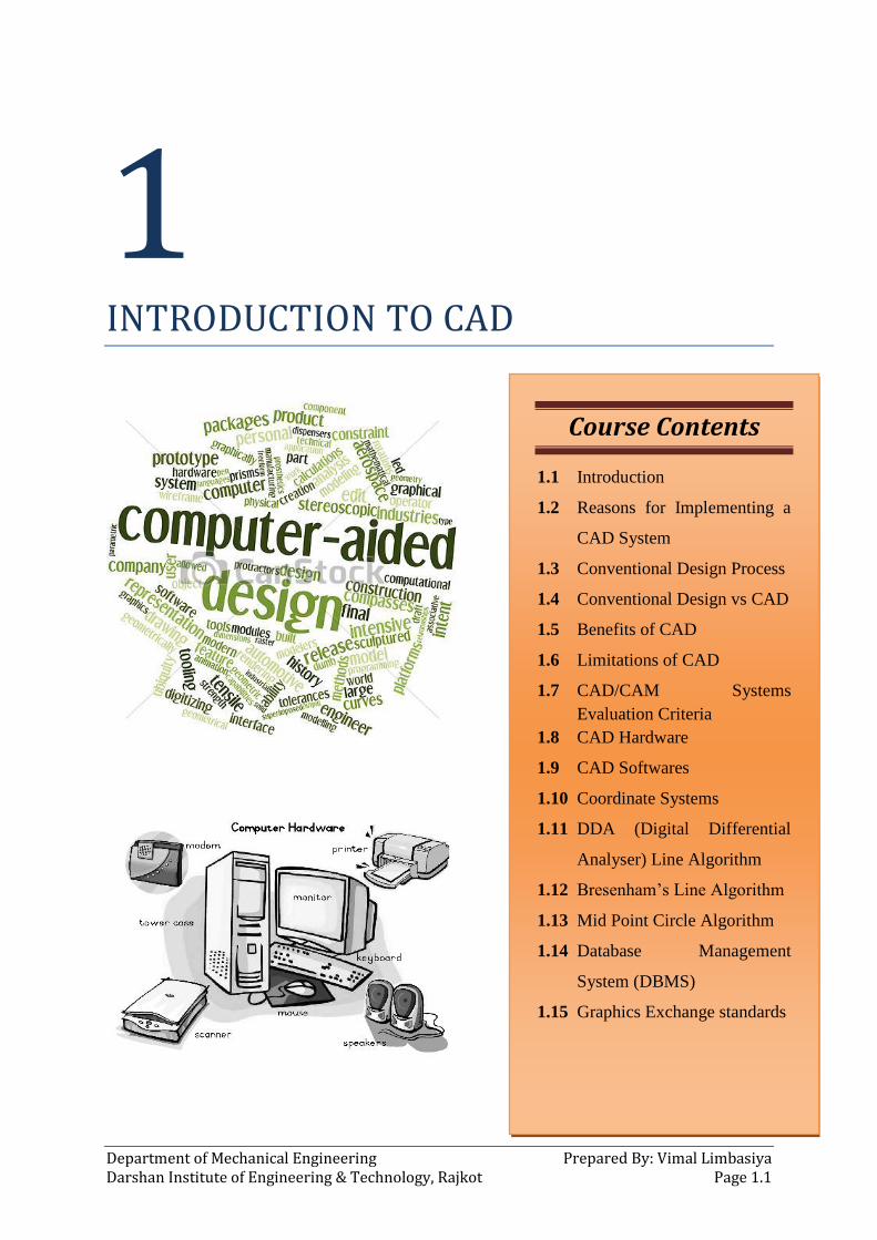
1 INTRODUCTION TO CAD
Course Contents
1.1 Introduction
1.2 Reasons for Implementing a
CAD System
1.3 Conventional Design Process
1.4 Conventional Design vs CAD
1.5 Benefits of CAD
1.6 Limitations of CAD
1.7 CAD/CAM Systems
Evaluation Criteria
1.8 CAD Hardware
1.9 CAD Softwares
1.10 Coordinate Systems
1.11 DDA (Digital Differential
Analyser) Line Algorithm
1.12 Bresenham’s Line Algorithm
1.13 Mid Point Circle Algorithm
1.14 Database Management
System (DBMS)
1.15 Graphics Exchange standards

1. Introduction to CAD Computer Aided Design (2161903)
Prepared By: Vimal Limbasiya Department of Mechanical Engineering Page 1.2 Darshan Institute of Engineering & Technology, Rajkot
1.1 Introduction
• In engineering practice, CAD/CAM has been utilized in different ways by different
people.
• Some utilize it to produce drawings and document designs.
• Others may employ it as a visual tool by generating shaded images and animated
displays.
• A third group may perform engineering analysis of some sort on geometric models
such as finite element analysis.
• A fourth group may use it to perform process planning and generate NC part
programs. In order to establish the scope and definition of CAD/CAM in an
engineering environment and identify existing and future related tools, a study of a
typical product cycle is necessary. Figure 1.1 shows a flowchart of such a cycle.
Fig. 1.1 Typical Product Cycle
• CAD tools can be defined as the intersection of three sets: geometrical modeling,
computer graphics and the design tools.
• Figure 1.2 shows such definition. As can be perceived from this figure, the abstracted
concepts of geometric modeling and computer graphics must be applied innovatively
to serve the design process.
• Based on implementation in a design environment, CAD tools can be defined as the
design tools (analysis codes, heuristic procedures, design practices, etc.) being
improved by computer hardware and software throughout its various phases to
achieve the design goal efficiently and competitively as shown in Fig. 1.2.
• The level of improvement determines the design capabilities of the various
CAD/CAM systems and the effectiveness of the CAD tools they provide.

Computer Aided Design (2161903) 1. Introduction to CAD
Department of Mechanical Engineering Prepared By: Vimal Limbasiya Darshan Institute of Engineering & Technology, Rajkot Page 1.3
• Designers will always require tools that provide them with fast and reliable solutions
to design situations that involve iterations and testings of more than one alternative.
• CAD tools can vary from geometric tools, such as manipulations of graphics entities
and interference checking, on one extreme, to customized applications programs,
such as developing analysis and optimization routines, on the other extreme.
• In between these two extremes, typical tools currently available include tolerance
analysis, mass property calculations and finite element modeling and analysis.
Fig. 1.2 Definition of CAD tools based on their Constituents
Fig. 1.3 Definition of CAD tools based on their implementation in a design environment
• CAD tools, as defined above, resemble guidance to the user of CAD technology.
• The definition should not and is not intended to, represent a restriction on utilizing it
in engineering design and applications. The principal purposes of this definition are
the following:
1. To extend the utilization of current CAD/CAM systems beyond just drafting
and visualization.
2. To customize current CAD/CAM systems to meet special design and analysis
needs.

1. Introduction to CAD Computer Aided Design (2161903)
Prepared By: Vimal Limbasiya Department of Mechanical Engineering Page 1.4 Darshan Institute of Engineering & Technology, Rajkot
3. To influence the development of the next generation of CAD/CAM systems to
better serve the design and manufacturing processes.
1.2 Reasons for Implementing a CAD System
1. To increase in the productivity of the designer
• The CAD improves the productivity of the designer to visualize the product and its
components, parts and reduces time required in synthesizing, analyzing and
documenting the design.
2. To improve the quality of design
• CAD system permits a more detailed engineering analysis and a large no. of design
alternatives can be investigated.
• The design errors are also reduced because of the greater accuracy provided by
system.
3. To improve communication in design
• The use of a CAD system provides better engineering drawings, more standardization
in drawing, better documentation of design, few drawing errors.
4. To create a data base for manufacturing
• In the process of creating the documentation for the product design, much of the
required data base to manufacture the product can be created.
5. Improves the efficiency of design
• It improves the efficiency of design process and the wastages at the design stage can
be reduced.
1.3 Conventional Design Process
Fig. 1.4 Conventional Design Process

Computer Aided Design (2161903) 1. Introduction to CAD
Department of Mechanical Engineering Prepared By: Vimal Limbasiya Darshan Institute of Engineering & Technology, Rajkot Page 1.5
There are six steps involved in the conventional design process as discussed below:
1. Recognition of need
• The first step in the designing process is to recognize necessity of that particular
design.
• The condition under which the part is going to operate and the operation of part in
that particular environment.
• The real problem is identified by knowing the history and difficulties faced in system.
2. Definition of problem
• The design involves type of shape of part, its space requirement, the material
restrictions and the condition under which the part has to operate.
• The basic purpose of design process has to be known before starting the design.
• A problem may be design of a simple part or complex part.
• It may be problem on optimizing certain parameters.
3. Synthesis of design
• In this, it may be necessary to prepare a rough drawing of design part.
• The type of loading conditions imposed on the parts.
• The type of shapes which the part section can require and approximate dimension at
which the different forces are located has to be provided on the sketch of part.
• The stresses to which the part is likely to be subjected must be analyzed and relevant
formulas should be prepared.
• A mathematical model of design may be prepared to synthesize the parts of design.
4. Analysis and optimization
• The design can be analyzed for the type of loading condition as well as the geometric
shape of the part.
• In the first stage it will be necessary to check the design of the part for safe stresses.
• If it is not satisfactory, then the dimensions of the part can be recalculated.
• The part can further be optimized for acquiring minimum dimensions, weight,
volume, efficiency of the material and cost.
• The optimization depends on the definition of the problem and importance of a
parameter.
• It may be sometimes necessary to optimize the parts for certain operating
parameters like efficiency, torque, etc.
5. Evaluation
• It is concerned with measuring the design against the specifications established in
the problem definition phase.
• The evaluation often requires the fabrication and testing of model to assess
operating performance, quality and reliability.
6. Presentation
• The design of component must be presented along with necessary drawings in an
attractive format.

1. Introduction to CAD Computer Aided Design (2161903)
Prepared By: Vimal Limbasiya Department of Mechanical Engineering Page 1.6 Darshan Institute of Engineering & Technology, Rajkot
• The presentation of the design can be made by use of colors and attractive
presentation.
1.4 Conventional Design vs CAD
Fig. 1.5 Computer Aided Design
1. Geometric modeling
• Geometric modeling is concerned with the computer compatible mathematical
description of the geometry of an object.
• The mathematical description allows the image of the object to be displayed and
manipulated on a graphics terminal through signals from the CPU of CAD system.
• The software that provides geometric modeling capabilities must be designed for
efficient use both by the computer and human designer.
• The basic form uses wire frames to represent the object.
• The most advanced method of geometric modeling is solid modeling in three
dimensions.
2. Engineering Analysis
• The analysis may involve stress-strain calculations, heat transfer computation etc.
• The analysis of mass properties is the analysis feature of CAD system that has
probably the widest application.
• It provides properties of solid object being analyzed, such as surface area, weight,
volume, center of gravity and moment of inertia.
• The most powerful analysis feature of CAD system is the finite element method.
Computer Aided Design (2161903) 1. Introduction to CAD
Department of Mechanical Engineering Prepared By: Vimal Limbasiya Darshan Institute of Engineering & Technology, Rajkot Page 1.7
3. Design Review & Analysis
• A procedure for design review is interference checking.
• This involves the analysis of an assembled structure in which there is a risk that the
components of the assembly may occupy same space.
• Most interesting evaluation features available on some CAD systems is kinematics.
• The available kinematics packages provide the capabilities to animate the motion of
simple designed mechanisms such as hinged components and linkages.
4. Automated Drafting
• This feature includes automatic dimensioning, generation of cross-hatched areas,
scaling of the drawing and the capability to develop sectional views and enlarged
views of particular part details.
1.5 Benefits of CAD
• Improved engineering productivity
• Reduced manpower required
• More efficient operation
• Customer modification are easier to make
• Low wastages
• Improved accuracy of design
• Better design can be evolved
• Saving of materials and machining time by optimization
• Colors can be used to customize the product
1.6 Limitations of CAD
• The system requires large memory and speed.
• The size of the software package is large.
• It requires highly skilled personal to perform the work.
• It has huge investment.
1.7 CAD/CAM Systems Evaluation Criteria
• The various types of CAD/CAM systems are Mainframe-Based Systems,
Minicomputer-Based Systems, Microcomputer-Based Systems and Workstation-
Based Systems.
• The implementation of these types by various vendors, software developers and hardware manufacturers result in a wide variety of systems, thus making the selection process of one rather difficult. CAD/CAM selection committees find themselves developing long lists of guidelines to screen available choices.
• These lists typically begin with cost criteria and end with sample models or benchmarks chosen to test system performance and capabilities. In between comes other factors such as compatibility requirements with in-house existing computers, prospective departments that plan to use the systems and credibility of CAD/CAM systems' suppliers.
1. Introduction to CAD Computer Aided Design (2161903)
Prepared By: Vimal Limbasiya Department of Mechanical Engineering Page 1.8 Darshan Institute of Engineering & Technology, Rajkot
• In contrast to many selection guidelines that may vary sharply from one organization to another, the technical evaluation criteria are largely the same. They are usually based on and are limited by the existing CAD/CAM theory and technology. These criteria can be listed as follows.
1.7.1. System Considerations
(i) Hardware
• Each workstation is connected to a central computer, called the server, which has
enough large disk and memory to store users' files and applications programs as well
as executing these programs.
(ii) Software
• Three major contributing factors are the type of operating system the software runs
under, the type of user interface (syntax) and the quality of documentation.
(iii) Maintenance
• Repair of hardware components and software updates comprise the majority of
typical maintenance contracts. The annual cost of these contracts is substantial
(about 5 to 10 percent of the initial system cost) and should be considered in
deciding on the cost of a system in addition to the initial capital investment.
(iv) Vendor Support and Service
• Vendor support typically includes training, field services and technical support. Most
vendors provide training courses, sometimes on-site if necessary.
1.7.2. Geometric Modeling Capabilities
(i) Representation Techniques
• The geometric modeling module of a CAD/CAM system is its heart. The applications
module of the system is directly related to and limited by the various
representations it supports. Wireframes, surfaces and solids are the three types of
modeling available.
(ii) Coordinate Systems and Inputs
• In order to provide the designer with the proper flexibility to generate geometric
models, various types of coordinate systems and coordinate inputs ought to be
provided. Coordinate inputs can take the form of cartesian (x, y, z), cylindrical (r, θ, z)
and spherical (θ, φ, z).
(iii) Modeling Entities
• The fact that a system supports a representation scheme is not enough. It is
important to know the specific entities provided by the scheme. The ease to
generate, verify and edit these entities should be considered during evaluation.
(iv) Geometric Editing and Manipulation
• It is essential to ensure that these geometric functions exist for the three types of
representations. Editing functions include intersection, trimming and projection and

Computer Aided Design (2161903) 1. Introduction to CAD
Department of Mechanical Engineering Prepared By: Vimal Limbasiya Darshan Institute of Engineering & Technology, Rajkot Page 1.9
manipulations include translation, rotation, copy, mirror, offset, scaling and changing
attributes.
(v) Graphics Standards Support
• If geometric models' databases are to be transferred from one system to another,
both systems must support exchange standards.
1.7.3. Design Documentation
(i) Generation of Engineering Drawings
• After a geometric model is created, standard drafting practices are usually applied to
it to generate the engineering drawings or the blueprints. Various views (usually top,
front and right side) are generated in the proper drawing layout. Then dimensions
are added, hidden lines are eliminated and/or dashed, tolerances are specified,
general notes and labels are added, etc.
1.7.4. Applications
(i) Assemblies or Model Merging
• Generating assemblies and assembly drawings from individual parts is an essential
process.
(ii) Design Applications
• There are design packages available to perform applications such as mass property
calculations, tolerance analysis, finite element modeling and analysis, injection
modeling analysis and mechanism analysis and simulation.
(iii) Manufacturing Applications
• The common packages available are tool path generation and verification, NC part
programming, postprocessing, computer aided process planning, group technology,
CIM applications and robot simulation.
(iv) Programming Languages Supported
• It is vital to look into the various levels of programming languages a system supports.
Attention should be paid to the syntax of graphics commands when they are used
inside and outside the programming languages. If this syntax changes significantly
between the two cases, user confusion and panic should be expected.
1.8 CAD Hardware
The hardware of CAD system consists of following:
• CPU
• Secondary memory
• Workstation
• Input unit
• Output unit
• Graphics display terminal
1. Introduction to CAD Computer Aided Design (2161903)
Prepared By: Vimal Limbasiya Department of Mechanical Engineering Page 1.10 Darshan Institute of Engineering & Technology, Rajkot
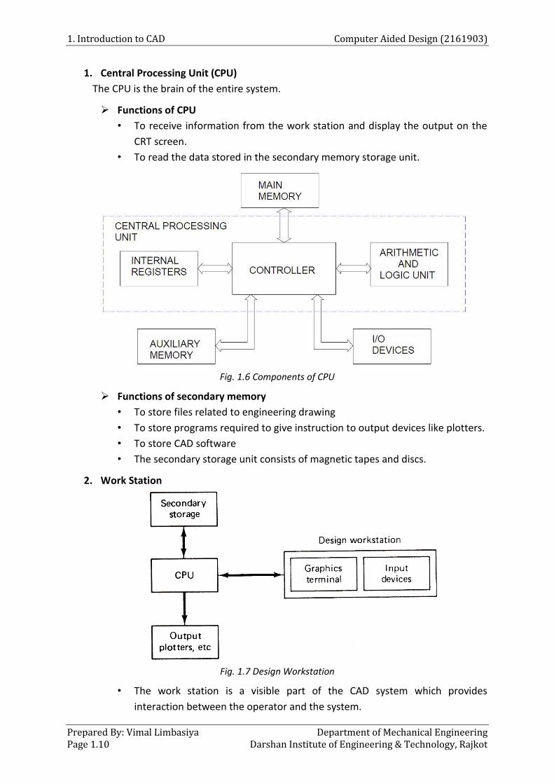
1. Central Processing Unit (CPU)
The CPU is the brain of the entire system.
Functions of CPU
• To receive information from the work station and display the output on the
CRT screen.
• To read the data stored in the secondary memory storage unit.
Fig. 1.6 Components of CPU
Functions of secondary memory
• To store files related to engineering drawing
• To store programs required to give instruction to output devices like plotters.
• To store CAD software
• The secondary storage unit consists of magnetic tapes and discs.
2. Work Station
Fig. 1.7 Design Workstation
• The work station is a visible part of the CAD system which provides
interaction between the operator and the system.

Computer Aided Design (2161903) 1. Introduction to CAD
Department of Mechanical Engineering Prepared By: Vimal Limbasiya Darshan Institute of Engineering & Technology, Rajkot Page 1.11
• Among these advantages offered by work station are their availability,
portability, the availability to dedicate them to a single task without affecting
other users and their consistency of time response.
• A work station can be defined as a station of work with its own computing
power to support major software packages, multitasking capabilities
demanded by increased usage, complex tasks and networking potential with
other computing environments.
Technical Specifications of CAD workstation
CAD applications require workstations with reasonably enhanced processing speed,
graphic capability, and storage capacity. Typical workstation specifications of some
of the currently available models are given below.
Processor: Intel Pentium 4 at 2.4 GHz
RAM: 2 GB to 16 GB
PCI bus width: 64 – bit
Hard drive: 500 GB to 1 TB
CD-ROM: CD-RW/DVD Combo
Standard I/O ports: 1 Serial port, 1 Parallel port, 4 USB ports
Graphics: NVIDIA 512 MB
Graphics Resolution: 2018 x 1536 (Max)
Operating System: Windows XP, Windows 7
Monitor: 21” Flat Panel TFT display
Keyboard: Enhanced Multimedia USB
Mouse: Optical Mouse Two-button Scroll Mouse
3. Input Devices
• A no. of input devices is available. These devices are used to input two
possible types of information: text and graphics.
• Text-input devices and the alphanumeric keyboards.
• There are two classes of graphics input devices: Locating devices and image-
input devices.
• Locating devices, or locators, provide a position or location on the screen.
• These include lightpens, mouse, digitizing tablets, joysticks, trackballs,
thumbwheels, touchscreen and touchpads.
• Locating devices typically operate by controlling the position of a cursor on
screen. Thus, they are also referred to as cursor-control devices.
I. Scanners
• Scanners comprise other class of graphics-input device.
• There are four relevant parameters to measure the performance of graphics
input devices. These are resolution, accuracy, repeatability and linearity.
• Some may be more significant to some devices than others.

1. Introduction to CAD Computer Aided Design (2161903)
Prepared By: Vimal Limbasiya Department of Mechanical Engineering Page 1.12 Darshan Institute of Engineering & Technology, Rajkot
II. Keyboards
• Keyboards are typically employed to create/edit programs or to perform
word processing functions.
• CAD/CAM systems, information entered through keyboards should be
displayed back to the user on a screen for verification.
III. Digitizing Tablets
Fig. 1.8 Digitizer
• A digitizing tablet is considered to be a locating as well as pointing device. It is
a small, low-resolution digitizing board often used in conjunction with a
graphics display.
• The tablet is a flat surface over which a stylus can be moved by the user.
• A tablet’s typical resolution is 200 dots per inch
• The tablet operation is based on sensitizing its surface area to be able to
track the pointing element motion on the surface.
• Several sensing methods and technologies are used in tablets. The most
common sensing technology is electromagnetic, where the pointing element
generates an out of phase magnetic field sensed by wire grid in tablet
surface.
IV. Mouse
Fig. 1.9 Mouse

Computer Aided Design (2161903) 1. Introduction to CAD
Department of Mechanical Engineering Prepared By: Vimal Limbasiya Darshan Institute of Engineering & Technology, Rajkot Page 1.13
• There are two basic types of mouse available mechanical and optical.
• The mechanical mouse has roller in order to record the mouse motion in X
and Y directions.
• In optical mouse, movements over the surface are measured by a light beam
modulation techniques.
• The light source is located at the bottom and the mouse must be in contact
with the surface for screen cursor to follow its movement.
V. Joy sticks & Trackballs
Fig. 1.10 Joy stick
• The joystick works by pushing its stick backwards or forward or to left or
right. The extreme positions of these directions correspond to the four corner
of the screen.
Fig. 1.11 Trackball
• A trackball is similar in principal to a joystick but allows more precise fingertip
control. The ball rotates freely within its mount.

1. Introduction to CAD Computer Aided Design (2161903)
Prepared By: Vimal Limbasiya Department of Mechanical Engineering Page 1.14 Darshan Institute of Engineering & Technology, Rajkot
• Both the joystick and trackball are used to navigate the screen display cursor.
The user of a trackball can learn quickly how to adjust to any nonlinearity in
its performance.
Fig. 1.12 (a) Cursor Control Devices (b) Thumbwheels as input device with a work station
VI. Thumbwheels
• Two thumbwheels are usually required to control the screen cursor, one for
its horizontal position and other for its vertical position. Each position is
indicated on screen by cross-hair.
4. Output Devices
CAD/CAM applications require output devices such as displays and hardcopy printers.
I. Graphics Displays
• The operation of CRT is based on concept of energizing an electron beam that
strikes the phosphor coating at very high speed.
• The energy transfer from the electron to the phosphor due to the impact
causes it to illuminate and glow.
• The electrons are generated via the electron gun that contains the cathode
and are focused into a beam via the focusing unit shown in Fig. 1.13.
• By controlling the beam direction and intensity in a way related to the
graphics information generated in the computer, meaningful and desired
graphics can be displayed on the screen.

Computer Aided Design (2161903) 1. Introduction to CAD
Department of Mechanical Engineering Prepared By: Vimal Limbasiya Darshan Institute of Engineering & Technology, Rajkot Page 1.15
Fig. 1.13 Principle of CRT
• The deflection system of the CRT controls the x and y, or the horizontal and
vertical, positions of the beam which in turn are related to the graphics
information through the display controller, which typically sits between the
computer and the CRT. The controller receives the information from the
computer and converts it into signals acceptable to the CRT.
Refresh vector display
Fig. 1.14 Refresh Display

1. Introduction to CAD Computer Aided Design (2161903)
Prepared By: Vimal Limbasiya Department of Mechanical Engineering Page 1.16 Darshan Institute of Engineering & Technology, Rajkot
• Early displays in 1960s were refresh vector displays.
• The refresh buffer stores the display file or program, which contains points,
lines, characters and other attributes of picture to be drawn.
• These commands are interpreted & processed by display processor.
• The electron beam accordingly excites the phosphor, which glows for a short
period.
• To maintain a steady flicker- free image, the screen must be refreshed or
redrawn at least 30 to 60 times per second, that is at a rate of 30 to 60 Hz.
• The principal advantages of refresh display is its high resolution (4096 x 4096)
and thus its generation of high quality picture.
Direct View Storage Tube (DVST)
Fig. 1.15 Direct View Storage Tube
• Refresh displays were very expensive in the 1960s, due to the required
refresh buffer memory and fast display processer.
• At the end of 1960s DVST was introduced by Tektronix as an alternative and
inexpensive solution.
• It uses a special type of phosphor that has long-lasting glowing effect.
• In the DVST, the picture is stored as a charge in the phosphor mesh located
behind the screen’s surface. Therefore, complex pictures could be drawn
without flicker at high resolution.

Computer Aided Design (2161903) 1. Introduction to CAD
Department of Mechanical Engineering Prepared By: Vimal Limbasiya Darshan Institute of Engineering & Technology, Rajkot Page 1.17
• Once displayed, the picture remains on the screen until it is erased. New
picture items can be added & displayed rapidly.
• However, if a displayed item is erased, the entire screen must be cleared and
new picture displayed to reflect removal of item.
Raster display
• The inability of the DVST to meet the increasing demands by various
CAD/CAM applications for colors, shaded images and animation motivated
hardware designers to continue searching for solution.
• In raster displays, display screen area is divided horizontally and vertically
into a matrix of small element called pixel.
• An N x M resolution defines a screen with N rows and M columns.
Fig. 1.16 Typical Pixel Matrix of a Raster Display
• Images are displayed by converting geometric information into pixel values
which are then converted into electron beam deflection through display
processors and deflection system.
• The creation of raster-format data from geometric information is known as
scan conversion.
• The values of the pixels of a display screen that results from scan-conversion
processes are stored in an area or memory called frame buffer or bit map.
• Each pixel value determines its brightness (gray level) or most often its color
on the screen.
• 8 bits/pixel are needed to produce satisfactory continuous shades of gray for
monochrome display.
• For color displays, 24 bits/pixel would be needed: 8 bits for each primary
color red, blue and green.
• This would provide 224 different colors, which are far more than needed in
real application.

1. Introduction to CAD Computer Aided Design (2161903)
Prepared By: Vimal Limbasiya Department of Mechanical Engineering Page 1.18 Darshan Institute of Engineering & Technology, Rajkot
Fig. 1.17 Color Raster Display with Eight Planes
• The bit map memory is arranged conceptually as a series of planes, one for
each bit in the pixel value. Thus an eight-plane memory provides 8 bits/pixel,
as shown in Fig. 1.17.
• This provides 28 different gray levels or different colors that can be displayed
simultaneously in one image. The number of bits per pixel directly affects the
quality of its display and consequently its price.
• The value of a pixel in the bit map memory is translated to a gray level or a
color through a lookup table (also called a color table or color map for a color
display).
(a) Monochrome display

Computer Aided Design (2161903) 1. Introduction to CAD
Department of Mechanical Engineering Prepared By: Vimal Limbasiya Darshan Institute of Engineering & Technology, Rajkot Page 1.19
(b) Color display
Fig. 1.18 Relationship between pixel value and a lookup table
• Figure 1.18 shows how the pixel value is related to the lookup table in an eight plane display. If cell P in the bit map corresponds to pixel P at the location P(x, y) on the screen, then the gray level of this pixel is 50 (00110010) or its corresponding color is 50.
• For color displays this may imply that the number of bits per pixel must be increased to increase the number of entries in the color map and therefore increase the available number of colors to the user.
• This, however, is not true and leads to increasing the size of the bit map memory and the cost of the display. Thus, how can the number of color indexes in the color map increase while keeping the pixel definition (number of bits per pixel) in the bit map to a minimum?
• For example, how can a display have 4 bits/pixel with 24 bits of color output (224 different colors)? This is achieved by designing a color map with 224 (16.7 million) available color indexes. The 4 bits/pixel provides 16 (24 simultaneous colors, in an image, which can be chosen from the color map.
• A pixel value (0 to 15) can be used to set the value of the color index which corresponds to the proper color to be displayed. This scheme, in this example, provides 16 simultaneous colors from a palette of 16.7 million.
• To the user, the color map is made available where colors are chosen and the application program relates the chosen color to the proper pixel value. For example, if the user chooses the color purple for an image element, the corresponding program sets the corresponding pixels to reflect the color purple.
Light Emitting Diode (LED)
• Light Emitting Diode (LED) is a emissive device. The emissive displays (or
emitters) are devices that convert electrical energy into light.
• A matrix of diodes is arranged to form the pixel positions in the display, and
picture definition is stored in a refresh buffer.

1. Introduction to CAD Computer Aided Design (2161903)
Prepared By: Vimal Limbasiya Department of Mechanical Engineering Page 1.20 Darshan Institute of Engineering & Technology, Rajkot
• As in scan – line refreshing of a CRT, information is read from the refresh
buffer and convert to voltage levels that are applied to the diodes to produce
the light pattern display.
Liquid Crystal Display (LCD) • Liquid crystals exist in a state between liquid and solid. The molecules of
liquid crystal are all aligned in the same direction, as in a solid, but are free to
move around slightly in relation to one another, as in a liquid.
• Liquid crystal is actually closer to a liquid state than a solid state, which is one
reason why it is rather sensitive to temperature.
• The array of liquid crystals become opaque when the electric field is applied,
for displaying the image. Their use as display devices has been made popular
by their widespread use in portable calculators and in the lap top or portable
computers.
• Their full screen size with reasonably low power consumption has made them
suitable for portability. Another advantage is that they occupy very small
desktop space while reducing the power consumption.
• The price of these displays is falling rapidly, and are thus becoming popular
for desk top applications as well. Also large screen size LCD monitors are
available currently at reasonable price.
II. Hardcopy Printers and Plotters
Output devices of both printers and plotters are available for producing final
drawings and documentation on paper.
Pen Plotters
• There are two types of conventional pen plotters flat bed and drum.
Fig. 1.19 Drum Plotter

Computer Aided Design (2161903) 1. Introduction to CAD
Department of Mechanical Engineering Prepared By: Vimal Limbasiya Darshan Institute of Engineering & Technology, Rajkot Page 1.21
• In the flat-bed plotter, the paper is stationary and the pen holding
mechanism can move in two axes.
Fig. 1.20 Flat-bed Plotter
Inkjet Plotters
• They utilize dot matrix method of plotting.
• Each dot is, however, created by impelling a tiny jet of ink on the
surface of the paper.
• Typical applications include color plots of solid models, shaded images
and contour plots.
Black and white Printers
• There are major two types of black and white printers are dot matrix
and laser printers.
• Dot matrix printers are inexpensive but slow.
Fig. 1.21 Dot Matrix Printer
• Their resolution is typically 75 dpi.
• Laser printers are more expensive but faster and better than dot
matrix printer.
• Their typical resolution is 300 dpi.

1. Introduction to CAD Computer Aided Design (2161903)
Prepared By: Vimal Limbasiya Department of Mechanical Engineering Page 1.22 Darshan Institute of Engineering & Technology, Rajkot
Laser printer
• A semiconductor laser beam scans the electro statically charged drum
with a rotating mirror.
• This writes on the drum a no. of points which are similar to pixels.
• When the beam strikes the drum in the wrong way round for printing
a positive charge, reversing it, then toner powder is released.
• The toner powder sticks to the charged positions of the drum, which
is then transformed to a sheet of paper.
• Though it is relatively expansive compared to the dot matrix printer,
the quality of the output is extremely good and it works very fast.
Fig. 1.22 Working of Laser Printer
1.9 CAD Softwares
• Softwares can be defined as an interpreter or translator which allows the user to
perform specific type of application or job related to CAD.
• The user may utilize the software for drafting or designing of machine parts or
components subjected to stresses or analysis of any type of system.
• The CAD application software can be prepared in variety of languages such as BASIC
(Beginner's All-purpose Symbolic Instruction Code), FORTRAN, Java, PASCAL & C-
Language.
• C- Language has been preferred for CAD software development because of no. of
advantages as compared to other languages.
• The Java language has the capacity to operate with high level graphics and
animation.
1.10 Coordinate Systems
Three types of coordinate systems are needed to input, store and display model
geometry and graphics. They are the world coordinate system (WCS), user
coordinate system (UCS) and screen coordinate system (SCS).

Computer Aided Design (2161903) 1. Introduction to CAD
Department of Mechanical Engineering Prepared By: Vimal Limbasiya Darshan Institute of Engineering & Technology, Rajkot Page 1.23
(i) World Coordinate System (WCS)
The world coordinate system is the reference space of the model with respect to
which all the model geometrical data is stored. Figure 1.23 shows a typical model,
which is to be modelled.
Figure 1.24(a) illustrates the model with its associated world coordinate system x, y,
and z. It is also called the model coordinate system. It is the default coordinate
system. The WCS is the only coordinate system that the software recognises when
storing or retrieving geometrical information.
(ii) User Coordinate System (UCS)
If the model has complex geometry the desired feature of construction can be easily
defined with respect to the world coordinate system.
It is often convenient in the development of geometric models and the input of data
with respect to an auxiliary coordinate system instead of WCS.
The user can define a Cartesian coordinate system whose xy plane is coincident with
the desired plane of construction. This coordinate system is called the user
coordinate system.
The UCS can be positioned at any position and orientation in the space that the user
desires. The user coordinate system is shown in Figure 1.24(b).
Fig. 1.23 Typical component to model.

1. Introduction to CAD Computer Aided Design (2161903)
Prepared By: Vimal Limbasiya Department of Mechanical Engineering Page 1.24 Darshan Institute of Engineering & Technology, Rajkot
Fig. 1.24 Coordinate systems.
(iii) Screen Coordinate System (SCS)
The screen coordinate system is a two-dimensional Cartesian coordinate system whose origin is located at the lower left corner of the graphics display (Figure 1.25). It is a device-dependent coordinate system.
For raster graphics displays, the pixel grid is the screen coordinate system. A 1024 x 1024 display as a range of (0, 0) to (1024, 1024). The centre of the screen is at (512, 512).
The SCS is used to display graphics by converting from WCS coordinates to SCS coordinates. The transformation from WCS coordinates to SCS coordinates is performed by the software before displaying the model views and graphics.
Fig. 1.25 Screen coordinate system.

Computer Aided Design (2161903) 1. Introduction to CAD
Department of Mechanical Engineering Prepared By: Vimal Limbasiya Darshan Institute of Engineering & Technology, Rajkot Page 1.25
1.11 DDA (Digital Differential Analyser) Line Algorithm
• DDA is one of the first algorithms developed for rasterizing the vectorial information.
The equation of a straight line is given by Equation 1.1
Y = m X + C (1.1)
• Using this equation for direct computing of the pixel positions involves a large
amount of computational effort.
• Hence it is necessary to simplify the procedure of calculating the individual pixel
positions by a simple algorithm.
• For this purpose consider drawing a line on the screen as shown in Fig. 1.26, from
(x1, y1) to (x2, y2),
Fig. 1.26 A straight Line Drawing by DDA algorithm
2 1
2 1
y ym
x x (1.2)
C = y1 – m x1 (1.3)
• The line drawing method would have to make use of the above three equations in
order to develop a suitable algorithm.
• Equation 1.1, for small increments can also be written as,
Y m X (1.4)
• By taking a small step for ∆X, ∆Y can be computed using Eq. 1.4. However, the
computations become unnecessarily long for arbitrary values of ∆X. Let us now
workout a procedure to simplify the calculation method.
• Let us consider a case of line drawing where 1m . Choose an increment for ∆X as
unit pixel. Hence ∆X = 1.
• Then from Eq. 1.4,
1i iy y m (1.5)
• The subscript i takes the values starting from 1 for the starting point till the end point
is reached.
• Hence it is possible to calculate the total pixel positions for completely drawing the
line on the display screen. This is called DDA (Digital Differential Analyser) algorithm.
• If m > 1, then the roles of x and y would have to be reversed.
• Choose

1. Introduction to CAD Computer Aided Design (2161903)
Prepared By: Vimal Limbasiya Department of Mechanical Engineering Page 1.26 Darshan Institute of Engineering & Technology, Rajkot
∆Y = 1 (1.6)
Then from Eq. 1.4, we get
1
1i ix x
m (1.7)
• The following is the flow chart showing the complete process for the implementation
of the above procedure.
Fig. 1.27 Flow chart for line calculation procedure by DDA algorithm
Example 1.1
Indicate which raster locations would be chosen by DDA algorithm when scan converting a
line from screen coordinate (19, 38) to screen coordinate (38, 52).
2 1
2 1
52 38 140.737
38 19 19
y y ym
x x x
So, 1m
∆X = 1 and 1i iy y m
Table 1.1 Calculation of pixel positions by DDA Algorithm
X Y calculated Y rounded
19 38 38
20 38.737 39
21 39.474 39

Computer Aided Design (2161903) 1. Introduction to CAD
Department of Mechanical Engineering Prepared By: Vimal Limbasiya Darshan Institute of Engineering & Technology, Rajkot Page 1.27
22 40.211 40
23 40.948 41
24 41.685 42
25 42.422 42
26 43.159 43
27 43.896 44
28 44.633 45
29 45.370 45
30 46.107 46
31 46.844 47
32 47.581 48
33 48.318 48
34 49.055 49
35 49.792 50
36 50.529 51
37 51.266 51
38 52.003 52
1.12 Bresenham’s Line Algorithm
• The above DDA algorithm is certainly an improvement over the direct use of the line
equation since it eliminates many of the complicated calculations.
• However, still it requires some amount of floating point arithmetic for each of the
pixel positions.
• This is still more expensive in terms of the total computation time since a large
number of points need to be calculated for each of the line segments as shown in
Example 1.1.
• Bresenham's method is an improvement over DDA since it completely eliminates the
floating point arithmetic except for the initial computations. All other computations
are fully integer arithmetic and hence it is more efficient for raster conversion.
• As for the DDA algorithm, start from the same line equation and the same
parameters. The basic argument for positioning the pixel here is the amount of
deviation by which the calculated position is from the actual position obtained by
the line equation in terms of d1 and d2 as shown in Fig. 1.28.
• Let the current position be (Xi, Yi) at the ith position as shown in Fig. 1.28. Each of the
circles in Fig. 1.28 represents the pixels in the successive positions.
• Then
1 1i ix x (1.8)
i iy mx C (1.9)
( 1)iy m x C (1.10)

1. Introduction to CAD Computer Aided Design (2161903)
Prepared By: Vimal Limbasiya Department of Mechanical Engineering Page 1.28 Darshan Institute of Engineering & Technology, Rajkot
Fig. 1.28 the Position of Individual Pixels for Calculation using Bresenham Procedure
• These are shown in Fig. 1.28. Let d1 and d2 be two parameters, which indicate where
the next pixel is to be located. If d1 is greater than d2, then the y pixel is to be located
at the +1 position else, it remains at the same position as previous location.
1 ( 1)i i id y y m x C y (1.11)
2 1 1 ( 1)i i id y y y m x C (1.12)
From Equations (1.11) & (1.12),
1 2 1( 1) ( 1)i i i id d m x C y y m x C (1.13)
1 2 2 ( 1) 2 2 1i id d m x C y (1.14)
• Equation 1.14 still contains more computations and hence we would now define
another parameter P which would define the relative position in terms of d1 – d2.
1 2( )iP d d x (1.15)
2 ( 1) 2 2 1i im x C y x
2 2 2 2i imx x m x C x y x x
2 2 2 2i i
y yx x x C x y x x
x x
y
mx
2 2 2 2i ix y y C x y x x (1.16)
2 2i i iP x y y x b (1.17)
, 2 2where b y C x x

Computer Aided Design (2161903) 1. Introduction to CAD
Department of Mechanical Engineering Prepared By: Vimal Limbasiya Darshan Institute of Engineering & Technology, Rajkot Page 1.29
• Similarly, we can write,
1 12 ( 1) 2 ( )i i iP y x x y b (1.18)
• Taking the difference of two successive parameters, we can eliminate the constant
terms from Eq. (1.18).
1 12 2 2 ( ) 2 2i i i i i iP P yx y x y yx xy
1 12 2 ( )i i i iP P y x y y (1.19)
• The same can also be written as
1 12 2 ( )i i i iP P y x y y (1.20)
• The same can also be written as
1 2i iP P y When yi+1 = yi (1.21)
1 2 2i iP P y x When yi+1 = yi +1 (1.22)
• From the start point (x1, y1)
1 1y mx C
1 1
yC y x
x
• Substituting this in Eq. 1.16 and simplifying, we get
1 1 1 1 12 2 2 2y
P x y y y x x y x xx
1 1 1 1 12 2 2 2 2P x y y y x x y y x x
1 2P y x (1.23)
• Hence from Eq. 1.19, when Pi is negative, then the next pixel location remains the
same as previous one and Eq. 1.21 becomes valid. Otherwise, Eq. 1.22 becomes
valid.
• Using these equations it is now possible to develop the algorithm for drawing the
line on the screen as shown in the flowchart (Fig. 1.29). The procedure just described
is for the case when 1m .
• The procedure can be repeated for the case when m > 1 by interchanging X and Y
similar to the DDA algorithm.

1. Introduction to CAD Computer Aided Design (2161903)
Prepared By: Vimal Limbasiya Department of Mechanical Engineering Page 1.30 Darshan Institute of Engineering & Technology, Rajkot
Fig. 1.29 Flow chart for line calculation procedure by Bresenham algorithm
Example 1.2
Indicate which raster locations would be chosen by Bresenham’s algorithm when scan
converting a line from screen coordinate (19, 38) to screen coordinate (38, 52).
2 1
2 1
52 38 140.737
38 19 19
y y ym
x x x
Table 1.2 Calculation of pixel positions by Bresenham’s Procedure
X P Y
19 P1 = 2∆y - ∆x = 28 – 19 = 9 38
20 P2 = P1 + 2∆y - 2∆x = 9 + 28 -38 = -1 39
21 P3 = P2 + 2∆y = -1 + 28 = 27 39
22 P4 = P3 + 2∆y - 2∆x = 27 + 28 -38 = 17 40
23 P5 = P4 + 2∆y - 2∆x = 17 + 28 -38 = 7 41
24 P6 = P5 + 2∆y - 2∆x = 7 + 28 -38 = -3 42

Computer Aided Design (2161903) 1. Introduction to CAD
Department of Mechanical Engineering Prepared By: Vimal Limbasiya Darshan Institute of Engineering & Technology, Rajkot Page 1.31
25 P7 = P6 + 2∆y = -3 + 28 = 25 42
26 P8 = P7 + 2∆y - 2∆x = 25 + 28 -38 = 15 43
27 P9 = P8 + 2∆y - 2∆x = 15 + 28 -38 = 5 44
28 P10 = P9 + 2∆y - 2∆x = 5 + 28 -38 = -5 45
29 P11 = P10 + 2∆y = -5 + 28 = 23 45
30 P12 = P10 + 2∆y - 2∆x = 23 + 28 -38 = 13 46
31 P13 = P12 + 2∆y - 2∆x = 13 + 28 -38 = 3 47
32 P14 = P13 + 2∆y - 2∆x = 3 + 28 -38 = -7 48
33 P15 = P14 + 2∆y = -7 + 28 = 21 48
34 P16 = P15 + 2∆y - 2∆x = 21 + 28 -38 = 11 49
35 P17 = P16 + 2∆y - 2∆x = 1 + 28 -38 = 1 50
36 P18 = P17 + 2∆y - 2∆x = 1 + 28 -38 = -9 51
37 P19 = P18 + 2∆y = -9 + 28 = 19 51
38 P20 = P19 + 2∆y - 2∆x = 19 + 28 -38 = 9 52
1.13 Mid point circle Algorithm
• As in the raster line algorithm, we sample at unit intervals and determine the closest
pixel position to the specified circle path at each step.
• For a given radius r and screen center position (xc, yc), we can first set up our
algorithm to calculate pixel positions around a circle path centered at the coordinate
origin (0,0).
• Then each calculated position (x,y) is moved to its proper screen position by adding
xc to x and yc to y. Along the circle section from x = 0 to x = y in the first quadrant,
the slope of the curve varies from 0 to -1.
• Therefore, we can take unit steps in the positive x direction over this octant and use
a decision Parameter to determine which of the two possible y positions is closer to
the circle path at each step. Positions in the other seven octants are then obtained
by symmetry.
• To apply the midpoint method, we define a circle function:
fcircle(x, y) = x2 + y2 – r2 (1.24)
• Any point (x, y) on the boundary of the circle with radius r satisfies the equation
fcircle(x, y) = 0. If the point is in the interior of the circle, the circle function is negative.
And if the point is outside the circle, the circle function is positive. To summarize, the
relative position of any point (x, y) can be determined by checking the sign of the
circle function:
0, if (x,y) is inside the circle boundary
( , ) = 0, if (x,y) is on the circle boundary
> 0, if (x,y) is outside the circle boundarycirclef x y
(1.25)
• The circle-function tests in Eq. 1.25 are performed for the midpositions between
pixels near the circle path at each sampling step. Thus, the circle function is the

1. Introduction to CAD Computer Aided Design (2161903)
Prepared By: Vimal Limbasiya Department of Mechanical Engineering Page 1.32 Darshan Institute of Engineering & Technology, Rajkot
decision parameter in the midpoint algorithm, and we can set up incremental
calculations for this function as we did in the line algorithm.
Fig. 1.30
• Figure 1.30 shows the midpoint between the two candidate pixels at sampling
position xk + 1.
• Assuming we have just plotted the pixel at (xk, yk), we next need to determine
whether the pixel at position (xk + 1, yk) or the one at position (xk + 1, yk - 1) is closer
to the circle. Our decision parameter is the circle function Eq. 1.24 evaluated at the
midpoint between these two pixels:
2
2 2
11,
2
11
2
k circle k k
k k
p f x y
x y r
(3-29)
• If Pk < 0, this midpoint is inside the circle and the pixel on scan line yk is closer to the
circle boundary. Otherwise, the midposition is outside or on the circle boundary, and
we select the pixel on scan line yk – 1.
• Successive decision parameters are obtained using incremental calculations. We
obtained a recursive expression for the next decision parameter by evaluating the
circle function at sampling position xk+1 + 1 = xk + 2:
1 1 1
22 2
1
11,
2
11 1
2
k circle k k
k k
p f x y
x y r
2 21 1 12 1 1k k k k k k kp p x y y y y
Where yk+1 is either yk or yk-1, depending on the sign of pk.
• Increments for obtaining
pk+1 = pk + 2xk+1 +1 (if pk is negative)
pk+1 = pk + 2xk+1 + 1 – 2yk+1
Evaluation of the terms 2xk+1, and 2yk+1 can also be done incrementally as

Computer Aided Design (2161903) 1. Introduction to CAD
Department of Mechanical Engineering Prepared By: Vimal Limbasiya Darshan Institute of Engineering & Technology, Rajkot Page 1.33
2xk+1 = 2xk + 2
2yk+1 = 2yk – 2
• At the start position (0, r), these two terms have the values 0 and 2r, respectively.
Each successive value is obtained by adding 2 to the previous value of 2x and
subtracting 2 from the previous value of 2y.
• The initial decision parameter is obtained by evaluating the circle function at the
start position (xo, yo) = (0, r):
2
2
11,
2
11
2
o circlep f r
r r
Or 5
4op r
• If the radius r is specified as an integer, we can simply round po to
po = 1 – r (for r an integer)
since all increments are integers.
1.14 Database Management System (DBMS)
A DBMS is defined as the software that allows access to use and/or modify data
stored in a database. The DBMS forms a layer of software between the physical
database itself (i.e., stored data) and the users of this database as shown in Fig.
1.31(a).
DBMS shields users from having to deal with hardware-level details by interpreting
their input commands and requests from the database. For example, a command
such as retrieve a line could involve few lower-level steps to execute.
Fig. 1.31 A typical DBMS
1. Introduction to CAD Computer Aided Design (2161903)
Prepared By: Vimal Limbasiya Department of Mechanical Engineering Page 1.34 Darshan Institute of Engineering & Technology, Rajkot
In general, a DBMS is responsible for all database-related activities such as creating
files, checking for illegal users of the database and synchronizing user access to the
database.
DBMSs designed for commercial business systems are too slow for CAD/ CAM. The
handling of graphics data is an area where the conventional DBMSs tend to break
down under the shear volume of data and the demand for quick display.
By contrast, data handled in the commercial realm is mostly alphanumeric and the
objects described are usually not very complex. A DBMS is directly related to the
database model it is supposed to manage. For example, relational DBMSs require
relatively large amounts of CPU time for searching and sorting data stored in the
relations or tables.
Therefore, the concept of database machines exists where a DBMS is implemented
into hardware that can lie between the CPU of a computer and its database disks, as
shown in Fig. 1.30(b).
1.15 Graphics Exchange standards
• With the proliferation of computers and software in the market, it became necessary
to standardize certain elements at each stage, so that investment made by
companies in certain hardware or software was not totally lost and could be used
without much modification on the newer and different systems.
• Standardization in engineering hardware is well known. Further, it is possible to
obtain hardware and software from a number of vendors and then be integrated
into a single system.
• This means that there should be compatibility between various software elements as
also between the hardware and software. This is achieved by maintaining proper
interface standards at various levels.
Both CAD/CAM vendors as well as users identified some needs to have some graphics
standards. The needs are as follows:
i. Software portability: This avoids hardware dependence of the software. If the
program is written originally for random scan display, when the display device is
changed to raster scan display the program should work with minimum effort.
ii. Image data portability: Information and storage of images should be independent of
different graphics devices.
iii. Text data portability: The text associated with graphics should be independent of
different input/output devices.
iv. Model database portability: Transporting of design and manufacturing data from
one application software to another should simple and economical.
The search for standards began in 1974 to fulfill the above needs both at the USA and
International levels. As a result of worldwide efforts, various standards at different levels of
the graphics systems were developed. The standards are as follows:

Computer Aided Design (2161903) 1. Introduction to CAD
Department of Mechanical Engineering Prepared By: Vimal Limbasiya Darshan Institute of Engineering & Technology, Rajkot Page 1.35
1. GKS (Graphics kernel system): It is an ANSI (American National Standards Institute
and ISO (International Standards Organization) standard. It interfaces the application
program with graphics support package.
2. IGES (Initial graphics exchange specification): It is an ANSI standard. It enables an
exchange of model database among CAD/CAM software.
3. PHIGS (Programmer's hierarchical interactive graphics system): It supports
workstations and their related CAD/CAM applications. It supports 3-dimensional
modeling of geometry segmentation and dynamic display.
4. CGM (Computer graphics metafile): It defines functions needed to describe an
image. Such description can be stored or transported from one graphics device to
another.
5. CGII (Computer graphics interface): It is designed to interface plotters to GKS or
PHIGS. It is the lowest device independent interface in a graphics system.
6. Drawing Exchange Format (DXF): The DXF format has been developed and
supported by Autodesk for use with the AutoCAD drawing files. It is not an industry
standard developed by any standards organisation, but in view of the widespread
use of AutoCAD made it a default standard for use of a variety of CAD/CAM vendors.
A Drawing Interchange File is simply an ASCII text file with a file extension of .DXF
and specially formatted text.
7. Standard for the Exchange of Product Model Data (STEP), officially the ISO standard
10303, Product Data Representation and Exchange, is a series of International
Standards with the goal of defining data across the full engineering and
manufacturing life cycle. The ability to share data across applications, across vendor
platforms and between contractors, suppliers and customers, is the main goal of this
standard.
8. Parasolid: It is a portable "kernel" that can be used in multiple systems - both high-
end and mid-range. By adopting Parasolid, start-up software companies have
eliminated a major barrier to application development - a high initial investment.
This enabled them to effectively market softwares with strong solid modeling
functionality at lower-cost.
9. PDES (Product Data Exchange Specification) is an exchange for product data in
support of industrial automation. "Product data" encompasses data relevant to the
entire life cycle of a product such as design, manufacturing, quality assurance,
testing and support. In order to support industrial automation, PDES files are fully
interpretable by computer. For example, tolerance information would be carried in a
form directly interpretable by a computer rather than a computerized text form
which requires human intervention to interpret.


Department of Mechanical Engineering Prepared By: Vimal G. Limbasiya Darshan Institute of Engineering & Technology, Rajkot Page 2.1
2 CURVES AND SURFACES
Course Contents
2.1 Curve representation
2.2 Classification of curves
2.3 Parametric representation of
analytical curves
2.3.1. Line
2.3.2. Circle
2.3.3. Ellipse
2.3.4. Parabola
2.3.5. Hyperbolas
2.4 Conics
2.5 Parametric representation of
synthetic curve
2.5.1. Hermite cubic spline
2.5.2. Bezier curves
2.5.3. B-spline curves
2.6 Surface modeling

2. Curves and Surfaces Computer Aided Design (2161903)
Prepared By: Vimal G. Limbasiya Department of Mechanical Engineering Page 2.2 Darshan Institute of Engineering & Technology, Rajkot
2.1 Curve Representation
Curve is defined as the locus of point moving with one degree freedom.
A curve can be represented by following two methods either by storing its analytical
equation or by storing an array of co-ordinates of various points
Curves can be described mathematically by following methods:
(i) Non-parametric form
a) Explicit form
b) Implicit form
(ii) Parametric form
2.1.1 Non-parametric form:
In this, the object is described by its co-ordinates with respect to current
reference frame in use.
2.1.1.1 Explicit form: (Clearly expressed)
In this, the co-ordinates of y and z of a point on curve are expressed as
two separate functions of x as independent variable.
P = [x y z]
= [x f(x) g(x)]
2.1.1.2 Implicit form: (Not clearly expressed)
In this, the co-ordinates of x, y and z of a point on curve are related
together by two functions.
F (x, y, z) = 0
G (x, y, z) = 0
Limitation of nonparametric representation of curves are:
1. If the slope of a curve at a point is vertical or near vertical, its value becomes infinity
or very large, a difficult condition to deal with both computationally and
programming-wise. Other ill-defined mathematical conditions may result.
2. Shapes of most engineering objects are intrinsically independent of any coordinate
system. What determines the shape of an object is the relationship between its data
points themselves and not between these points and some arbitrary coordinate
system.
3. If the curve is to be displayed as a series of points or straight line segments, the
computations involved could be extensive.
2.1.2 Parametric form:
In this, a parameter is introduced and the co-ordinates of x, y and z are
expressed as functions of this parameters. This parameter acts as a local
co-ordinate for points on curve.
P (u) = [x y z]
= [x (u) y (u) z (u)]

Computer Aided Design (2161903) 2. Curves and Surfaces
Department of Mechanical Engineering Prepared By: Vimal G.Limbasiya Darshan Institute of Engineering & Technology, Rajkot Page 2.3
2.2 Classification of Curves
Curves can be classified as shown below mainly in two categories:
1. Analytical Curves:
The curves which are defined by the analytical equations are known as analytical
curves.
Examples: line, circle, ellipse, parabola, hyperbola etc.
2. Synthetic Curves:
The curves which are defined by set of data points are known as synthetic curves.
Combination of polynomial segments to represent a desired curve is called a
synthetic curve.
These curves can be conveniently twisted, shaped or bent by changing the
control points.
Examples: Cubic spline curve, B-spline curve, Bezier curve etc.
Synthetic curves take up where the analytic curves leave – the latter are not that
efficient at geometric design of mechanical parts.
Need for synthetic curves arise in two occasions:
When a curve is represented by a collection of measured data points,
When an existing curve must change to meet new design requirements
the designer needs a curve representation that is directly related to the
data points and is flexible enough to bend, twist or change the shape by
changing one or more data points.
Some examples of complex geometric design are: Car bodies, Ship hulls, Airplane
fuselage and wings, Propeller blades, Shoe insoles, aesthetically designed bottles
etc.
When the curve pass through all the data points, then the curve is known as
Interpolant curve. It sounds more logical but can be more unstable and ringing.
When a smooth curve is approximated through the data points, then the curve is
known as approximation curve. It turns out to be convenient.
(a) Interploation
(b) Approximation
Fig. 2.1 Interpolant and Approximated Curves

2. Curves and Surfaces Computer Aided Design (2161903)
Prepared By: Vimal G. Limbasiya Department of Mechanical Engineering Page 2.4 Darshan Institute of Engineering & Technology, Rajkot
Synthetic curve pass through defined data points and can thus represented by
polynomial equations.
The parametric form for any synthetic curve is:
3 23 2 1 0P u C u C u C u C
where, u = Parameter and Ci = Polynomial coefficients
2.3 Parametric representation of analytical curve
Lines
A line can be represented in a parametric form by an input of two endpoints or by
one point and a length and direction. Besides these, modifiers and filters can be used
to represent these lines. The two important methods of establishing equations for
lines are considered.
A line connecting two endpoints in parametric form, having the values of
parameter u as 0 and 1 at the endpoints:
Fig. 2.2 Line between Two Endpoints
Consider a line between two given endpoints P1 (x1, y1, z1) and P2(x2, y2, z2) as shown
in Fig. 2.2. The position vectors for these two points would be P1 and P2. Consider any
point P (x, y, z) on the line P1 P2.
Let a parametric system be introduced such that the point P is represented by the
parameter u such that its values are 0 and 1 at endpoints P1 and P2 respectively.
From ∆OPP1, we can express the vector between endpoints P1 and P as P - P1. This
vector represents the parameter u. The mapping between the Cartesian and
parametric space can be done by the following relation :
1
1
Distance of P from P in cartesian space Endpoint Length in cartesian space
Distance of P from P in parametric space Endpoint Length in parametric space

Computer Aided Design (2161903) 2. Curves and Surfaces
Department of Mechanical Engineering Prepared By: Vimal G.Limbasiya Darshan Institute of Engineering & Technology, Rajkot Page 2.5
1 2 1
1
P P P P
u
1 2 1P P u P P
1 2 1P P u P P where, 0 ≤ u ≤ 1
This equation represents the vector equation of the line in parametric form. In scalar
form, it can be written as:
1 2 1x x u x x
1 2 1y y u y y
1 2 1z z u z z where, 0 ≤ u ≤ 1
Any point on the above line or its extension can be found by substituting the value of
parameter u. The tangent vector of the line would be represented by :
2 1'P P P
In scalar form these would have the coordinates expressed by the following
equations:
2 1'x x x
2 1'y y y
2 1'z z z
It can be seen that the tangent vector is independent of the parameter u, thus
representing the constant slope of the line. Above equations are sufficient to
represent all properties of the line for CAD/CAM representation. The length L and
direction vector n
can be calculated using the following equations :
2 1L P P
2 2 2
2 1 2 1 2 1x x y y z z
2 1P Pn
L
A line passing through a point and defined by a length and direction:
Consider a case, where a line is to pass through a point P1 and has its length L and
direction vector n
defined as input as shown in Fig. 2.3. The computation of the
endpoint of this line needs to be done based on the above inputs. As seen earlier,
1P Pn
L
1P P L n
where, - ∞ ≤ L ≤ ∞
Once the user inputs P1, L and n
, the endpoint can be calculated as per the above
equation. The two endpoints can then be expressed in parametric form with values
of parameter u as 0 and 1.

2. Curves and Surfaces Computer Aided Design (2161903)
Prepared By: Vimal G. Limbasiya Department of Mechanical Engineering Page 2.6 Darshan Institute of Engineering & Technology, Rajkot
Fig. 2.3 Line passing through a point and defined by a Length and Direction
Parallel Lines
Fig. 2.4
Assume that the existing line has the two endpoints P1 and P2, a length L1, and a
direction defined by the unit vector 1
n . The new line has the same direction 1
n , a
length L2 and endpoints P3 and P4.
The unit vector 1
n is given by
2 1
1
P Pn
L
The unit vector for the parallel line will be same as unit vector for the existing line.

Computer Aided Design (2161903) 2. Curves and Surfaces
Department of Mechanical Engineering Prepared By: Vimal G.Limbasiya Darshan Institute of Engineering & Technology, Rajkot Page 2.7
4 3
2
P Pn
L
4 3 2P P L n
The equation of parallel line becomes,
3 4 3P P u P P
Angle between two lines
Fig. 2.5
Fig. 2.5 represents two lines L1 and L2 having endpoints are P1, P2 and P3, P4, the angle measurement command uses the equation
2 1 4 3
2 1 4 3
( ) ( )cos
| || |
P P P P
P P P P
cosθ = L1 . L2
Distance of a point from line
Fig. 2.6
Fig. 2.6 shows the distance D from point P3 to the line whose endpoints are P1 and P2
and direction is
n . Its length is L. D is given by
3 13 1 3 1
3 1
( )( ) ( )
| |
P PD P P n P P
P P

2. Curves and Surfaces Computer Aided Design (2161903)
Prepared By: Vimal G. Limbasiya Department of Mechanical Engineering Page 2.8 Darshan Institute of Engineering & Technology, Rajkot
Example 2.1: For the position vectors P1[1 2] and P2[4 3], determine the parametric
representation of line segment between them. Also determine the slope and tangent vector
of line segment.
A parametric representation of line is
1 2 1P P u P P
= [1 2] + u ([4 3] – [1 2])
= [1 2] + u [3 1]
Parametric representation of x and y components are
x(u) = x1 + u (x2 – x1)
= 1 + 3u
y(u) = y1 + u (y2 – y1)
= 2 + u
The tangent vector is obtained by differentiating P(u)
P’(u) = *x’(u) y’(u)+
= [3 1]
The slope of line segment is
/
/
dy dy du
dx dx du
'
'
y
x
1
3
Example 2.2 : The end points of line are P1(1,3,7) and P2(–4,5, –3). Determine
i. Tangent vector of the line
ii. Length of line
iii. Unit vector in the direction of line
Parametric representation of x, y and z components are
x(u) = x1 + u (x2 – x1)
= 1 – 5u
y(u) = y1 + u (y2 – y1)
= 3 + 2u
z(u) = z1 + u (z2 – z1)
= 7 – 10u
Tangent vector, P’(u) = *x’(u) y’(u) z’(u)+
= [–5 2 –10]
= –5i + 2j –10k
Length of line, 2 1L P P
2 2 2
2 1 2 1 2 1x x y y z z

Computer Aided Design (2161903) 2. Curves and Surfaces
Department of Mechanical Engineering Prepared By: Vimal G.Limbasiya Darshan Institute of Engineering & Technology, Rajkot Page 2.9
2 2 2
4 1 5 3 3 7
= 11.358
2 1 2 1
2 1
Unit vector in the direction of line,
1 [ 5 2 10]
11.358
P P P Pn
P P L
= [–0.44 0.176 –0.88]
= –0.44i + 0.176j –0.88k
Example 2.3: A line is represented by the end point P1(2, 4, 6) and P2(-3, 6, 9). If the value of
parameter u at P1 and P2 is 0 and 1 respectively, determine the tangent vector for the line. Also
determine the coordinate of a point represented by; u equal to 0, 0.25, -0.25, 1 and 1.5. Also find the
length and unit vector of line between two points P1 and P2.
Parametric representation of x, y and z components are
x(u) = x1 + u (x2 – x1)
= 2 – 5u
y(u) = y1 + u (y2 – y1)
= 4 + 2u
z(u) = z1 + u (z2 – z1)
= 6 – 3u
Tangent vector, P’(u) = *x’(u) y’(u) z’(u)+
= [–5 2 –3]
= –5i + 2j –3k
u 0 0.25 – 0.25 1 1.5
x (u) 2 0.75 3.25 –3 –5.5
y (u) 4 4.5 3.5 6 7
z (u) 6 5.25 6.75 3 1.5
Length of line, 2 1L P P
2 2 2
2 1 2 1 2 1x x y y z z
2 2 2
3 2 6 4 9 6
= 6.16
2 1 2 1
2 1
Unit vector in the direction of line,
1 [ 5 2 3]
6.16
P P P Pn
P P L
= [–0.81 0.324 –0.487]
= –0.81i + 0.324j –0.487k
2. Curves and Surfaces Computer Aided Design (2161903)
Prepared By: Vimal G. Limbasiya Department of Mechanical Engineering Page 2.10 Darshan Institute of Engineering & Technology, Rajkot
Circles
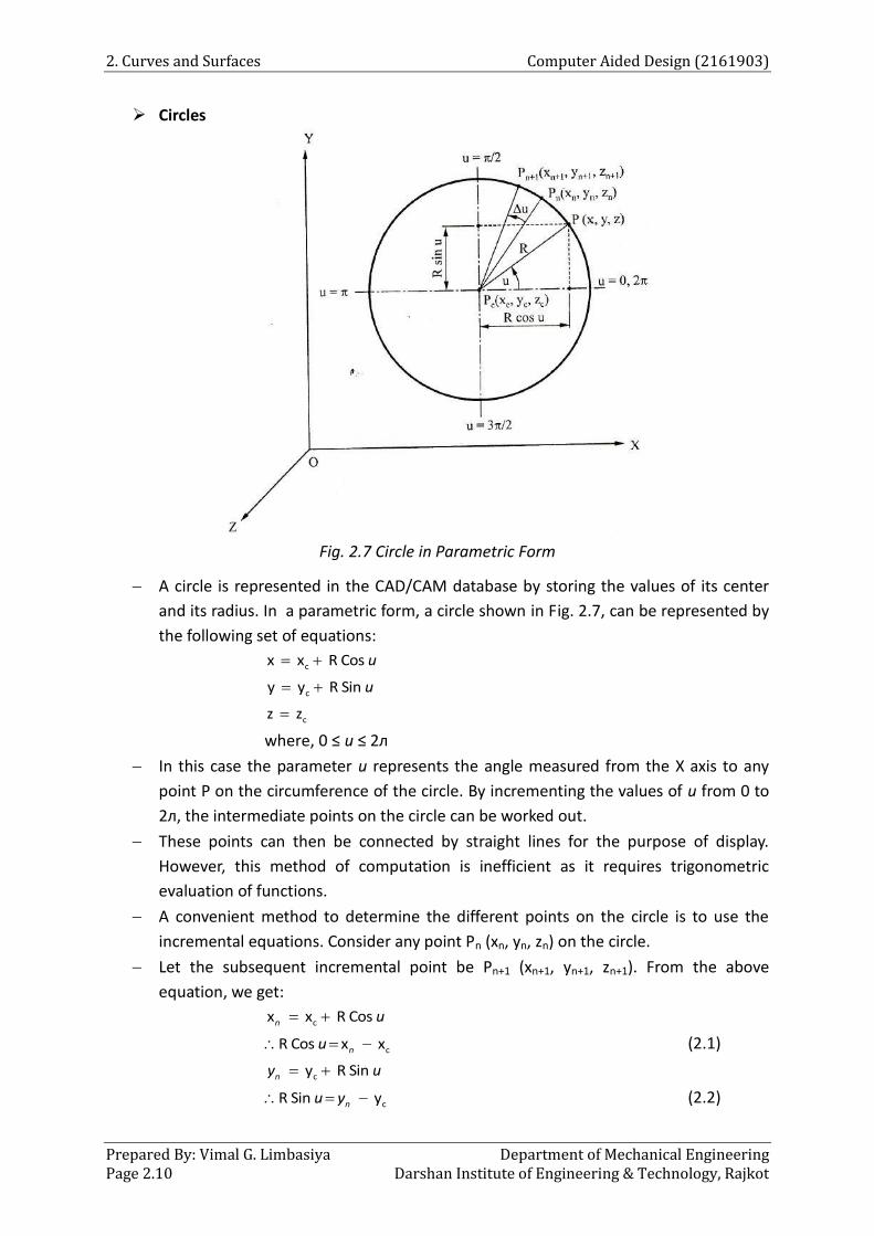
Fig. 2.7 Circle in Parametric Form
A circle is represented in the CAD/CAM database by storing the values of its center
and its radius. In a parametric form, a circle shown in Fig. 2.7, can be represented by
the following set of equations:
cx x R Cos u
cy y R Sin u
cz z
where, 0 ≤ u ≤ 2ᴫ
In this case the parameter u represents the angle measured from the X axis to any
point P on the circumference of the circle. By incrementing the values of u from 0 to
2ᴫ, the intermediate points on the circle can be worked out.
These points can then be connected by straight lines for the purpose of display.
However, this method of computation is inefficient as it requires trigonometric
evaluation of functions.
A convenient method to determine the different points on the circle is to use the
incremental equations. Consider any point Pn (xn, yn, zn) on the circle.
Let the subsequent incremental point be Pn+1 (xn+1, yn+1, zn+1). From the above
equation, we get:
cx x R Cos n u
cR Cos x xnu (2.1)
c y R Sin ny u
cR Sin ynu y (2.2)
Computer Aided Design (2161903) 2. Curves and Surfaces
Department of Mechanical Engineering Prepared By: Vimal G.Limbasiya Darshan Institute of Engineering & Technology, Rajkot Page 2.11
Similarly, 1 cx x R Cos n u u (2.3)
1 c y R Sin ny u u (2.4)
1 nz zn (2.5)
From (2.3), (2.1) & (2.2)
1 cx x R Cos Cos R Sin Sin n u u u u
1 c c cx x x x Cos y y Sin n n nu u (2.6)
From (2.4), (2.1) & (2.2)
1 c y R Sin Cos R Cos Sin ny u u u u
1 c c c y y y Cos x x Sin n n ny u u (2.7)
And 1z zn c
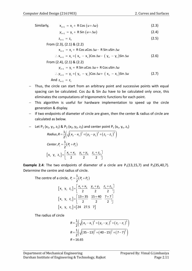
Thus, the circle can start from an arbitrary point and successive points with equal
spacing can be calculated. Cos ∆u & Sin ∆u have to be calculated only once, this
eliminates the computations of trigonometric functions for each point.
This algorithm is useful for hardware implementation to speed up the circle
generation & display.
If two endpoints of diameter of circle are given, then the center & radius of circle are
calculated as below.
Let P1 (x1, y1, z1) & P2 (x2, y2, z2) and center point Pc (xc, yc, zc)
2 2 2
2 1 2 1 2 1
1,
2Radius R x x y y z z
1 2
1,
2cCenter P P P
1 2 1 2 1 2c c cx y z
2 2 2
x x y y z z
Example 2.4: The two endpoints of diameter of a circle are P1(13,15,7) and P2(35,40,7).
Determine the centre and radius of circle.
The centre of a circle, 1 2
1
2cP P P
1 2 1 2 1 2c c c
c c c
c c c
x y z2 2 2
13 35 15 40 7 7x y z
2 2 2
x y z 24 27.5 7
x x y y z z
The radius of circle
2 2 2
2 1 2 1 2 1
2 2 2
1
2
135 13 40 15 7 7
2
16.65
R x x y y z z
R
R

2. Curves and Surfaces Computer Aided Design (2161903)
Prepared By: Vimal G. Limbasiya Department of Mechanical Engineering Page 2.12 Darshan Institute of Engineering & Technology, Rajkot
Ellipse
Mathematically the ellipse is a curve generated by a point moving in space such that
at any position the sum of its distances from two fixed points (foci) is constant and
equal to the major diameter. Each focus is located on the major axis of the ellipse at a
distance from its center equal to 2 2A B (A and B are the major and minor radii).
Circular holes and forms become ellipses when they are viewed obliquely relative to
their planes.
Fig. 2.8 Ellipse Defined by a Center, Major and Minor Axes
However, four conditions (points and/or tangent vectors) are required to define the
geometric shape of an ellipse.
Fig. 2.8 shows an ellipse with point Pc as the center and the lengths of half of the
major and minor axes are A and B respectively. The parametric equation of an ellipse
can be written as assuming the plane of the ellipse is the XY plane.
The parameter u is the angle as in the case of a circle. However, for a point P shown
in the figure, it is not the angle between the line PPc and the major axis of the ellipse.
Instead, it is defined as shown.
To find point P on the ellipse that corresponds to an angle u, the two concentric
circles C1 and C2 are constructed with centers at Pc and radii of A and B respectively. A
radial line is constructed at the angle u to intersect both circles at points P1 and P2
respectively.

Computer Aided Design (2161903) 2. Curves and Surfaces
Department of Mechanical Engineering Prepared By: Vimal G.Limbasiya Darshan Institute of Engineering & Technology, Rajkot Page 2.13
If a line parallel to the minor axis is drawn from P1 and a line parallel to the major axis
is drawn from P2, the intersection of these two lines defines the point P.
cos
sin 0 2c
c
c
x x A u
y y B u u
z z
Similar development as in the case of a circle results in the following recursive
relationships which are useful for generating points on the ellipse for display
purposes without excessive evaluations of trigonometric functions:
1
1
1
( ) cos ( ) sin
( ) cos ( ) sin
n c n c n c
n c n c n c
n n
Ax x x x u y y u
BA
y y y y u x x uB
z z
(2.8)
If the ellipse major axis is inclined with an angle α relative to the x axis as shown in
Fig. 2.8, the ellipse equation becomes
cos cos sin sin
cos sin sin cos 0 2c
c
c
x x A u B u
y y A u B u u
z z
(2.9)
Equations (2.9) cannot be reduced to a recursive relationship similar to what is given
by Eqs. (2.8). Instead these equations can be written as
1
1
1
cos( ) cos sin( ) sin
cos( ) sin sin( ) cosn c n n
n c n n
n n
x x A u u B u u
y y A u u B u u
z z
Parabola
The parabola is defined mathematically as a curve generated by a point that moves
such that its distance from a fixed point (the focus PF) is always equal to its distance
to a fixed line (the directrix) as shown in Fig. 2.9.
The vertex Pv is the intersection point of the parabola with its axis of symmetry. It is
located midway between directrix and focus. Focus lies on the axis of symmetry.
Useful applications of the parabolic curve in engineering design include its use in
parabolic sound and light reflectors, radar antennas and in bridge arches.
Three conditions are required to define a parabola, a parabolic curve, or a parabolic
arc. The default plane of a parabola is the XY plane of the current WCS at the time of
construction.
The database of a parabola usually stores the coordinates of its vertex, distances yHW
and yLW, that define its endpoints as shown in Fig. 2.9, the distance A between the
focus and the vertex (the focal distance) and the orientation angle α.
Unlike the ellipse, the parabola is not a closed curve. Thus, the two endpoints
determine the amount of the parabola to be displayed.
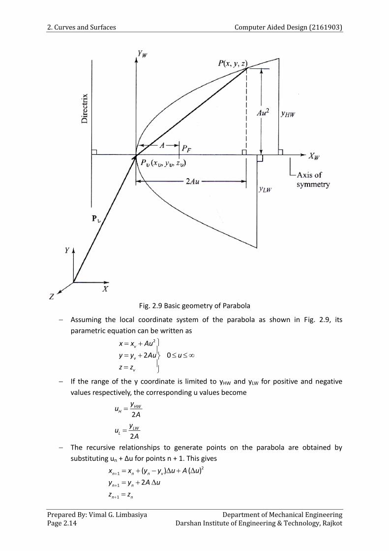
2. Curves and Surfaces Computer Aided Design (2161903)
Prepared By: Vimal G. Limbasiya Department of Mechanical Engineering Page 2.14 Darshan Institute of Engineering & Technology, Rajkot
Fig. 2.9 Basic geometry of Parabola
Assuming the local coordinate system of the parabola as shown in Fig. 2.9, its
parametric equation can be written as 2
2 0v
v
v
x x Au
y y Au u
z z
If the range of the y coordinate is limited to yHW and yLW for positive and negative
values respectively, the corresponding u values become
2
HWH
yu
A
2
LWL
yu
A
The recursive relationships to generate points on the parabola are obtained by
substituting un + Δu for points n + 1. This gives
21
1
1
( ) ( )
2n n n v
n n
n n
x x y y u A u
y y A u
z z

Computer Aided Design (2161903) 2. Curves and Surfaces
Department of Mechanical Engineering Prepared By: Vimal G.Limbasiya Darshan Institute of Engineering & Technology, Rajkot Page 2.15
Hyperbolas
A hyperbola is described mathematically as a curve generated by a point moving such
that at any position the difference of its distances from the fixed points (foci) F and F'
is a constant and equal to the transverse axis of the hyperbola.
Fig. 2.10 Hyperbola Geometry
Fig. 2.10 shows the geometry of a hyperbola.
The parametric equation of a hyperbola is given by
cosh
sinhv
v
v
x x A u
y y B u
z z
This equation is based on the nonparametric implicit equation of the hyperbola
which can be written as 2 2
2 2
( ) ( )1v vx x y y
A B
by utilizing the identity cosh2u – sinh2u = 1.
2.4. Conics
Conic curves or conic sections form the most general form of quadratic curves. Lines,
circles, ellipses, parabolas and hyperbolas are all special forms of conic curves. They
all can be generated when a right circular cone of revolution is cut by planes at
different angles relative to the cone axis-thus the derivation of the name conics.
Straight lines result from intersecting a cone with a plane parallel to its axis and
passing through its vertex. Circles results when the cone is sectioned by a plane
perpendicular to its axis while ellipses, parabolas and hyperbolas are generated when
the plane is inclined to the axis by various angles.

2. Curves and Surfaces Computer Aided Design (2161903)
Prepared By: Vimal G. Limbasiya Department of Mechanical Engineering Page 2.16 Darshan Institute of Engineering & Technology, Rajkot
2.5. Parametric representation of synthetic curve
Analytic curves, are usually not sufficient to meet geometric design requirements of
mechanical parts. Products such as car bodies, ship hulls, airplane fuselage and
wings, propeller blades, shoe insoles and bottles are a few examples that require
free-form, or synthetic, curves and surfaces.
The need for synthetic curves in design arises on two occasions: when a curve is
represented by a collection of measured data points and when an existing curve must
change to meet new design requirements.
In the latter occasion, the designer would need a curve representation that is directly
related to the data points and is flexible enough to bend, twist, or change the curve
shape by changing one or more data points.
Data points are usually called control points and the curve itself is called an
interpolant if it passes through all the data points.
Fig. 2.11 Various Orders of Continuity of Curves
Mathematically, synthetic curves represent a curve-fitting problem to construct a
smooth curve that passes through given data points. Therefore, polynomials are the
typical form of these curves.
Various continuity requirements can be specified at the data points to impose various
degrees of smoothness of the resulting curve. The order of continuity becomes
important when a complex curve is modeled by several curve segments pieced
together end to end.
Zero-order continuity (C0) yields a position continuous curve. First (C1)- and second
(C2)-order continuities imply slope and curvature continuous curves respectively.
Computer Aided Design (2161903) 2. Curves and Surfaces
Department of Mechanical Engineering Prepared By: Vimal G.Limbasiya Darshan Institute of Engineering & Technology, Rajkot Page 2.17
A C1 curve is the minimum acceptable curve for engineering design. Fig. 2.11 shows a
geometrical interpretation of these orders of continuity.
A cubic polynomial is the minimum order polynomial that can guarantee the
generation of C0, C1, or C2 curves. In addition, the cubic polynomial is the lowest-
degree polynomial that permits inflection within a curve segment and that allows
representation of nonplanar (twisted) three dimensional curves in space.
Higher-order polynomials are not commonly used in CAD/CAM because they tend to
oscillate about control points, are computationally inconvenient and are
uneconomical of storing curve and surface representations in the computer.
The type of input data and its influence on the control of the resulting synthetic
curve determine the use and effectiveness of the curve in design.
For example, curve segments that require positions of control points and/or tangent
vectors at these points are easier to deal with and gather data for than those that
might require curvature information.
Also, the designer may prefer to control the shape of the curve locally instead of
globally by changing the control point(s). If changing a control point results in
changing the curve locally in the vicinity of that point, local control of the curve is
achieved; otherwise global control results.
Major CAD/CAM systems provide three types of synthetic curves: Hermite cubic
spline, Bezier and B-spline curves. The cubic spline curve passes through the data
points and therefore is an interpolant.
Bezier and B-spline curves in general approximate the data points, that is, they do
not pass through them. Under certain conditions, the B-spline curve can be an
interpolant. Both the cubic spline and Bezier curves have a first-order continuity and
the B-spline curve has a second-order continuity.
Hermite Cubic Spline Curve:
They are used to interpolate the given data but not to design free-form curves.
Splines derive their name from “French curves or splines”
It connects two data (end) points and utilizes a cubic equation.
Four conditions are required to determine the coefficients of the equation – two end
points and the two tangent vectors at these two points.
It passes through the control points and therefore it is an Interpolant. It has only up
to C1 continuity.
The curve cannot be modified locally, i.e., when a data point is moved, the entire
curve is affected, resulting in a global control.
The order of the curve is always constant (cubic), regardless of the number of data
points. Increase in the number of data points increases shape flexibility, however, this
requires more data points, creating more splines that are joined together (only two
data points and slopes are utilized for each spline).

2. Curves and Surfaces Computer Aided Design (2161903)
Prepared By: Vimal G. Limbasiya Department of Mechanical Engineering Page 2.18 Darshan Institute of Engineering & Technology, Rajkot
Fig. 2.12 Hermite Cubic Spline Curve
A cubic spline curve utilizes a cubic equation of the following form:
(2.10)
where, 0 ≤ u ≤ 1
The cubic spline is defined by the two endpoints P0, P1 and the tangent vectors at
these points. The tangent vector can be found by differentiating equ.(2.10).
23 2 1' 3 2P u C u C u C (2.11)
To determine the coefficients of the curve, consider the two endpoints P0, P1 and the
tangent vectors as shown in Fig. 2.12.
Applying conditions at u = 0, in equations (2.10) and (2.11)
0 0P C (2.12)
0 1'P C (2.13)
Applying conditions at u = 1, in equations (2.10) and (2.11)
1 3 2 1 0P C C C C (2.14)
1 3 2 1' 3 2P C C C (2.15)
Substituting (2.12) and (2.13) in (2.14) and (2.15), we get:
1 3 2 0 0'P C C P P (2.16)
1 3 2 0' 3 2 'P C C P (2.17)
By solving simultaneous equations (2.16) and (2.17), we get
1 1 2 0 03 ' 2 ' 3P P C P P
2 1 1 0 03 ' 2 ' 3C P P P P (2.18)
Similarly again by solving simultaneous equations (2.16) and (2.17), we get
1 1 3 0 0' 2 ' 2P P C P P
3 1 1 0 0' 2 ' 2C P P P P (2.19)
Substituting (2.12), (2.13), (2.18) and (2.19) in (2.10), we get:
3 23 2 1 0P u C u C u C u C

Computer Aided Design (2161903) 2. Curves and Surfaces
Department of Mechanical Engineering Prepared By: Vimal G.Limbasiya Darshan Institute of Engineering & Technology, Rajkot Page 2.19
3 21 1 0 0 1 1 0 0 0 0' 2 ' 2 3 ' 2 ' 3 'P u P P P P u P P P P u P u P
3 3 3 3 2 2 2 21 1 0 0 1 1 0 0 0 0' 2 ' 2 3 ' 2 ' 3 'P u P u Pu P u P u Pu P u P u P u P u P
3 2 3 2 3 2 3 20 0 0 1 1 0 0 0 1 12 3 2 3 ' 2 ' ' ' 'P u P u P u P Pu Pu P u P u P u P u P u
3 2 3 2 3 2 3 20 1 0 12 3 1 2 3 ' 2 'P u P u u P u u P u u u P u u (2.20)
The expression can be written in matrix form as under:
3 2
3 2
0 1 0 1 3 2
3 2
2 3 1
2 3' '
2
u u
u uP u P P P P
u u u
u u
3
2
0 1 0 1
2 3 0 1
2 3 0 0' '
1 2 1 0
1 1 0 0 1
u
uP u P P P P
u
On similar lines, the tangent vector equation can be determined by differentiating
equation (2.20)
2 2 2 20 1 0 1' 6 6 6 6 ' 3 4 1 ' 3 2P u P u u P u u P u u P u u
2
2
0 1 0 1 2
2
6 6
6 6' ' '
3 4 1
3 2
u u
u uP u P P P P
u u
u u
3
2
0 1 0 1
0 6 6 0
0 6 6 0' ' '
0 3 4 1
0 3 2 0 1
u
uP u P P P P
u
Changing the values of endpoints or tangent vectors would modify the shape of the
curve.
Example 2.5: A cubic spline curve has start point P0(16,0) and end point P1(3,1). The tangent
vector for end point P0 is given by line joining P0 and point P2(14,8). Tangent vector for end
P1 is given by line joining P2 and point P1.
1. Determine the parametric equation of hermite cubic curve.
2. Plot the hermite cubic curve.
P0 = [16 0]
P1 = [3 1]
P’0 = P2 – P0 = [14 8] – [16 0]
= [–2 8]
P’1 = P1 – P2 = [3 1] – [14 8]
= [–11 –7]

2. Curves and Surfaces Computer Aided Design (2161903)
Prepared By: Vimal G. Limbasiya Department of Mechanical Engineering Page 2.20 Darshan Institute of Engineering & Technology, Rajkot
Parametric equation
For any point on curve
3
2
0 1 0 1
2 3 0 1
2 3 0 0' '
1 2 1 0
1 1 0 0 1
u
uP u P P P P
u
X coordinate of a point on curve
3
2
0 1 0 1
2 3 0 1
2 3 0 0' '
1 2 1 0
1 1 0 0 1
x x x x x
u
uP u P P P P
u
3
2
2 3 0 1
2 3 0 016 3 2 11
1 2 1 0
1 1 0 0 1
x
u
uP u
u
3
2
13 24 2 16
1
x
u
uP u
u
3 213 24 2 16xP u u u u
Y coordinate of a point on curve
3
2
0 1 0 1
2 3 0 1
2 3 0 0' '
1 2 1 0
1 1 0 0 1
y y y y y
u
uP u P P P P
u
3
2
2 3 0 1
2 3 0 00 1 8 7
1 2 1 0
1 1 0 0 1
y
u
uP u
u
3
2
1 6 8 0
1
y
u
uP u
u
3 2 8yP u u u u
Thus, parametric equation of parametric curve is
3 2
3 2
13 24 2 16
8
x
y
P u u u u
P u u u u
(2.21)

Computer Aided Design (2161903) 2. Curves and Surfaces
Department of Mechanical Engineering Prepared By: Vimal G.Limbasiya Darshan Institute of Engineering & Technology, Rajkot Page 2.21
Curve plot
The point on curve obtained by varying value of u from 0 to 1 in steps of 0.1 in equ. (2.21)
are shown in table
Point
No. 0 1 2 3 4 5 6 7 8 9 10
U 0 0.1 0.2 0.3 0.4 0.5 0.6 0.7 0.8 0.9 1
x (u) 16 15.57 14.74 13.59 12.19 10.63 8.97 7.30 5.70 4.24 3.00
y (u) 0 0.74 1.35 1.83 2.18 2.38 2.42 2.32 2.05 1.61 1.00
The Hermite cubic curve plotted using the above coordinates is shown in Fig. 2.13.
Fig. 2.13
Example 2.6: The end point of a cubic spline curve are P0(1,2) and P1(7,1). The tangent vector
for end P0 is given by line joining P0 and point P2(-2,1). The tangent vector for end P0 is given
by line joining P3(9,-2) and point P1.
1. Determine the parametric equation of hermite cubic curve.
2. Determine the parametric equation for tangent vector.
3. Plot the hermite cubic curve.
P0 = [1 2]
P1 = [7 1]
P’0 = P2 – P0 = [–2 1] – [1 2] = [–3 –1]
P’1 = P1 – P3 = [7 1] – [9 –2] = [–2 3]

2. Curves and Surfaces Computer Aided Design (2161903)
Prepared By: Vimal G. Limbasiya Department of Mechanical Engineering Page 2.22 Darshan Institute of Engineering & Technology, Rajkot
Parametric equation of curve
For any point on curve
3
2
0 1 0 1
2 3 0 1
2 3 0 0' '
1 2 1 0
1 1 0 0 1
u
uP u P P P P
u
X coordinate of a point on curve
3
2
0 1 0 1
2 3 0 1
2 3 0 0' '
1 2 1 0
1 1 0 0 1
x x x x x
u
uP u P P P P
u
3
2
2 3 0 1
2 3 0 01 7 3 2
1 2 1 0
1 1 0 0 1
x
u
uP u
u
3
2
17 26 3 1
1
x
u
uP u
u
3 217 26 3 1xP u u u u
Y coordinate of a point on curve
3
2
0 1 0 1
2 3 0 1
2 3 0 0' '
1 2 1 0
1 1 0 0 1
y y y y y
u
uP u P P P P
u
3
2
2 3 0 1
2 3 0 02 1 1 3
1 2 1 0
1 1 0 0 1
y
u
uP u
u
3
2
4 4 1 2
1
y
u
uP u
u
3 24 4 2yP u u u u
Thus, parametric equation of parametric curve is
3 2
3 2
17 26 3 1
4 4 2
x
y
P u u u u
P u u u u
(2.22)

Computer Aided Design (2161903) 2. Curves and Surfaces
Department of Mechanical Engineering Prepared By: Vimal G.Limbasiya Darshan Institute of Engineering & Technology, Rajkot Page 2.23
Parametric equation of tangent vector
3
2
0 1 0 1
0 6 6 0
0 6 6 0' ' '
0 3 4 1
0 3 2 0 1
u
uP u P P P P
u
X coordinate of tangent vector
3
2
0 6 6 0
0 6 6 0' 1 7 3 2
0 3 4 1
0 3 2 0 1
x
u
uP u
u
3
2
' 0 51 52 3
1
x
u
uP u
u
2' 51 52 3xP u u u
Y coordinate of tangent vector
3
2
0 6 6 0
0 6 6 0' 2 1 1 3
0 3 4 1
0 3 2 0 1
y
u
uP u
u
3
2
' 0 12 8 1
1
y
u
uP u
u
2' 12 8 1yP u u u
Thus, parametric equation of tangent vector is
2
2
' 51 52 3
' 12 8 1
x
y
P u u u
P u u u
Curve plot
The point on curve obtained by varying the value of u from 0 to 1 in steps of 0.1 in equ.(2.22)
are shown in table
Point
No. 0 1 2 3 4 5 6 7 8 9 10
U 0 0.1 0.2 0.3 0.4 0.5 0.6 0.7 0.8 0.9 1
x (u) 1 0.94 1.30 1.98 2.87 3.88 4.89 5.81 6.54 6.97 7.00
y (u) 2 1.86 1.67 1.45 1.22 1.00 0.82 0.71 0.69 0.78 1.00

2. Curves and Surfaces Computer Aided Design (2161903)
Prepared By: Vimal G. Limbasiya Department of Mechanical Engineering Page 2.24 Darshan Institute of Engineering & Technology, Rajkot
The Hermite cubic curve plotted using the above coordinates is shown in Fig. 2.14.
Fig. 2.14
Bezier Curves:
Cubic splines are based on interpolation techniques. Curves resulting from these
techniques pass through the given points.
Another alternative to create curves is to use approximation techniques which
produce curves that do not pass through the given data points. Instead, these
points are used to control the shape of the resulting curves.
Most often, approximation techniques are preferred over interpolation techniques
in curve design due to the added flexibility and the additional intuitive feel
provided by the former. Bezier and B-spline curves are examples based on
approximation techniques.
As its mathematics show shortly, the major differences between the Bezier curve
and the cubic spline curve are:
1. The shape of Bezier curve is controlled by its defining points only. First derivatives
are not used in the curve development as in the case of the cubic spline. This
allows the designer a much better feel for the relationship between input (points)
and output (curve).
2. The order or the degree of Bezier curve is variable and is related to the number of
points defining it; n + 1 points define an nth degree curve which permits higher-
order continuity. This is not the case for cubic splines where the degree is always
cubic for a spline segment.

Computer Aided Design (2161903) 2. Curves and Surfaces
Department of Mechanical Engineering Prepared By: Vimal G.Limbasiya Darshan Institute of Engineering & Technology, Rajkot Page 2.25
3. The Bezier curve is smoother than the cubic spline because it has higher order
derivatives.
Fig. 2.15 Beizer Curve
The Bezier curve is defined in terms of (n+1) points. This points are called as
control points, where n is the degree of the curve.
If n=3 control points are 4, as shown in the Fig 2.15.
These control points form the vertices of the control polygon or Bezier
characteristic polygon.
The control or Bezier characteristic polygon uniquely defines the curve.
Properties of Beizer Curve:
The degree of polynomial defining the curve segment is one less than the no. of
defining polygon points (n-1).
The curve follows the shape of the defining polygon.
Only the first and last control points or vertices of polygon actually lie on curve.
The other vertices define order & shape of the curve. (see Fig. 3.8)
Fig. 2.16 Same data points but different orders for Beizer Curve
The curve is also always tangent to first and last segments of polygon.
The same Beizer curve would be generated, if the sequence of the points is
changed from P0 – P1 – P2 – P3 to P3 – P2 – P1 – P0.
The flexibility of the shape would increase with increase in number of vertices
of the polygon.
It is having global control on the shape of the curve.

2. Curves and Surfaces Computer Aided Design (2161903)
Prepared By: Vimal G. Limbasiya Department of Mechanical Engineering Page 2.26 Darshan Institute of Engineering & Technology, Rajkot
Fig. 2.17 Same Typical Examples of Beizer Curve
Mathematically, for n + 1 control points, the Bezier curve is defined by the
following polynomial of degree n:
,0
P( ) P ( ), 0 1n
i i ni
u B u u
(2.23)
where P(u) is any point on the curve and Pi is a control point. Bi,n are the Bernstein
polynomials. Thus, the Bezier curve has a Bernstein basis. The Bernstein polynomial
serves as the blending or basis function for the Bezier curve and is given by
, ( ) ( , ) (1 )i n ii nB u C n i u u (2.24)
where C(n,i) is the binomial coefficient
!
( , )! !
nC n i
i n i
(2.25)
Utilizing Eqs. (2.24) and (2.25) and observing that C(n, 0) = C(n, n) = 1,
Eq. (2.23) can be expanded to give 1 2 2
0 1 2
11
P( ) P (1 ) P ( ,1) (1 ) P ( ,2) (1 )
..... P ( , 1) (1 ) P , 0 1
n n n
n nn n
u u C n u u C n u u
C n n u u u u
Bezier curve with 3 control points 2 2 1 2 2 2
0 1 2
2 20 1 2
P( ) P (1 ) P (2,1) (1 ) P (2,2) (1 )
P( ) (1 ) P 2 (1 )P P
u u C u u C u u
u u u u u
Bezier curve with 4 vertices 3 3 1 2 3 2 3 3 3
0 1 2 3
3 2 2 30 1 2 3
P( ) P (1 ) P (3,1) (1 ) P (3,2) (1 ) P (3,3) (1 )
P( ) (1 ) P 3 (1 ) P 3 (1 )P P
u u C u u C u u C u u
u u u u u u u

Computer Aided Design (2161903) 2. Curves and Surfaces
Department of Mechanical Engineering Prepared By: Vimal G.Limbasiya Darshan Institute of Engineering & Technology, Rajkot Page 2.27
Bezier curve with 5 vertices 4 4 1 2 4 2 3 4 3 4 4 4
0 1 2 3 4
4 3 2 2 3 40 1 2 3 4
P( ) P (1 ) P (4,1) (1 ) P (4,2) (1 ) P (4,3) (1 ) P (4,4) (1 )
P( ) (1 ) P 4 (1 ) P 6 (1 ) P 4 (1 )P P
u u C u u C u u C u u C u u
u u u u u u u u u
Example 2.7: A Bezier curve is to be constructed using control points P0(35,30), P1(25,0),
P2(15,25) and P3(5,10). The Bezier curve is anchored at P0 and P3. Find the equation of the
Bezier curve and plot the curve for u = 0, 0.2, 0.4, 0.6, 0.8 and 1.
P0 = [35 30]
P1 = [25 0]
P2 = [15 25]
P3 = [5 10]
n = 3
The parametric equation for Bezier curve 3 2 2 3
0 1 2 3P( ) (1 ) P 3 (1 ) P 3 (1 )P Pu u u u u u u
X-coordinate of a point on curve 3 2 2 3
0 1 2 3
3 2 2 3
2 3 2 2 3 3
2 3 2 3 2 3 3
P ( ) (1 ) P 3 (1 ) P 3 (1 )P P
P ( ) 35(1 ) 75 (1 ) 45 (1 ) 5
P ( ) 35(1 3 3 ) 75 (1 2 ) 45 45 5
P ( ) 35 105 105 35 75 150 75 45 45 5
P ( ) 35 30
x x x x x
x
x
x
x
u u u u u u u
u u u u u u u
u u u u u u u u u u
u u u u u u u u u u
u u
Y-coordinate of a point on curve 3 2 2 3
0 1 2 3
3 2 3
2 3 2 3 3
2 3
P ( ) (1 ) P 3 (1 ) P 3 (1 )P P
P ( ) 30(1 ) 75 (1 ) 10
P ( ) 30(1 3 3 ) 75 75 10
P ( ) 30 90 165 95
y y y y y
y
y
y
u u u u u u u
u u u u u
u u u u u u u
u u u u
The parametric equation of Bezier curve
2 3
P ( ) 35 30
P ( ) 30 90 165 95
x
y
u u
u u u u
(2.26)
The points on curve obtained by varying the value of u = 0, 0.2, 0.4, 0.6, 0.8 and 1 in equ.
(2.26) are shown in below table
Point No. 0 2 4 6 8 10
u 0 0.2 0.4 0.6 0.8 1
Px (u) 35.0 29.0 23.0 17.0 11.0 5.00
Py (u) 30.0 17.84 14.32 14.88 14.96 10.00
The Bezier curve plotted using the above coordinates is shown in Fig. 2.18.

2. Curves and Surfaces Computer Aided Design (2161903)
Prepared By: Vimal G. Limbasiya Department of Mechanical Engineering Page 2.28 Darshan Institute of Engineering & Technology, Rajkot
Fig. 2.18
Example 2.8: Plot a Bezier curve using the following control points.
(2,0), (4,3), (5,2), (4,-2), (5,-3) and (6,-2).
P0 = [2 0] P1 = [4 3]
P2 = [5 2] P3 = [4 -2]
P4 = [5 -3] P5 = [6 -2]
n = 5
The parametric equation for Bezier curve with 6 control points 5 4 2 3 3 2 4 5
0 1 2 3 4 5P( ) (1 ) P 5 (1 ) P 10 (1 ) P 10 (1 ) P 5 (1 )P Pu u u u u u u u u u u
2 3 4 5 2 3 40 1
2 2 3 3 2 4 52 3 4 5
P( ) (1 5 10 10 5 )P 5 (1 4 6 4 )P
10 (1 3 3 )P 10 (1 2 )P 5 (1 )P P
u u u u u u u u u u u
u u u u u u u u u u
2 3 4 5 2 3 4 50 1
2 3 4 5 3 4 5 4 5 52 3 4 5
P( ) (1 5 10 10 5 )P (5 20 30 20 5 )P
(10 30 30 10 )P (10 20 10 )P (5 5 )P P
u u u u u u u u u u u
u u u u u u u u u u
2 30 0 1 0 1 2 0 1 2 3
4 50 1 2 3 4 0 1 2 3 4 5
P( ) P ( 5P 5P ) (10P 20P 10P ) ( 10P 30P 30P 10P )
(5P 20P 30P 20P 5P ) ( P 5P 10P 10P 5P P )
u u u u
u u
X-coordinate of a point on a curve 2 3
0 0 1 0 1 2 0 1 2 3
4 50 1 2 3 4 0 1 2 3 4 5
P ( ) P ( 5P 5P ) (10P 20P 10P ) ( 10P 30P 30P 10P )
(5P 20P 30P 20P 5P ) ( P 5P 10P 10P 5P P )
x x x x x x x x x x x
x x x x x x x x x x x
u u u u
u u

Computer Aided Design (2161903) 2. Curves and Surfaces
Department of Mechanical Engineering Prepared By: Vimal G.Limbasiya Darshan Institute of Engineering & Technology, Rajkot Page 2.29
2 3
4 5
P ( ) 2 ( 5(2) 5(4)) (10(2) 20(4) 10(5)) ( 10(2) 30(4) 30(5) 10(4))
(5(2) 20(4) 30(5) 20(4) 5(5)) ( (2) 5(4) 10(5) 10(4) 5(5) (6))
x u u u u
u u
2 3 4 5P ( ) 2 10 10 10 25 11x u u u u u u
Y-coordinate of a point on a curve 2 3
0 0 1 0 1 2 0 1 2 3
4 50 1 2 3 4 0 1 2 3 4 5
P ( ) P ( 5P 5P ) (10P 20P 10P ) ( 10P 30P 30P 10P )
(5P 20P 30P 20P 5P ) ( P 5P 10P 10P 5P P )
y y y y y y y y y y y
y y y y y y y y y y y
u u u u
u u
2 3
4 5
P ( ) 0 ( 5(0) 5(3)) (10(0) 20(3) 10(2)) ( 10(0) 30(3) 30(2) 10( 2))
(5(0) 20(3) 30(2) 20( 2) 5( 3)) ( (0) 5(3) 10(2) 10(2) 5( 3) ( 2))
y u u u u
u u
2 3 4 5P ( ) 15 40 10 25 12y u u u u u u
The parametric equation of Bezier curve 2 3 4 5
2 3 4 5
P ( ) 2 10 10 10 25 11
P ( ) 15 40 10 25 12
x
y
u u u u u u
u u u u u u
(2.27)
The points on curve obtained by varying the value of u from 0 to 1 in steps of 0.1 in
equ.(2.27) are shown in below table
Point No. 0 1 2 3 4 5 6 7 8 9 10
u 0 0.1 0.2 0.3 0.4 0.5 0.6 0.7 0.8 0.9 1
Px (u) 2 2.89 3.56 4.01 4.29 4.47 4.62 4.82 5.12 5.52 6.00
Py (u) 0 1.11 1.52 1.34 0.76 -0.06 -0.93 -1.68 -2.17 -2.29 -2.00
Fig. 2.19

2. Curves and Surfaces Computer Aided Design (2161903)
Prepared By: Vimal G. Limbasiya Department of Mechanical Engineering Page 2.30 Darshan Institute of Engineering & Technology, Rajkot
B-Spline Curve:
B-Spline curves are proper and powerful generalization of Bezier curve.
They are very similar to Bezier curve and are also defined with the help of
characteristic polygon.
The major advantage of B-Spline curve is due to its ability to control the curve
shape locally, as opposed to global control (see Fig. 2.20).
Fig. 2.20 Local Control of a B-Spline Curve
B-Spline curves allow a local control over the shape of the spline curve.
B-Spline curves allow us to vary the control points without changing the degree of
the polynomial (i.e. number of control points can be added or subtracted).
The degree of the curve is independent of the number of control points (i.e. four
control points can generate a linear, quadratic or cubic curve).
It gives better control over the shape of curve.
They are more complex compared to Bezier curves.
B-spline curve defined by n + 1 control points P i is given by
, max0
P( ) P ( ), 0n
i i ki
u N u u u
(2.28)
Ni,k(u) are the B-spline functions. Thus, the B-spline curves have a B-spline basis.

Computer Aided Design (2161903) 2. Curves and Surfaces
Department of Mechanical Engineering Prepared By: Vimal G.Limbasiya Darshan Institute of Engineering & Technology, Rajkot Page 2.31
Rational curves
A rational curve is defined by the algebraic ratio of two polynomials while a
nonrational curve is defined by one polynomial.
The formulation of rational curves requires the introduction of homogeneous
space and the homogeneous coordinates. The homogeneous space is four-
dimensional space. A point in three dimensional with coordinates (x, y, z) is
represented in the homogeneous space by the coordinates (x*, y*, z*, h),where h
is a scalar factor. The relationship between the two types of coordinates is
* * *x y zx y z
h h h
A rational B-spline curve defined by n + 1 control points Pi is given by
, max0
P( ) P ( ), 0n
i i ki
u R u u u
(2.29)
Ri,k(u) are the rational B-spline functions and are given by
,,
,0
( )( )
( )
i i ki k n
i i ki
h N uR u
h N u
The above equation shows that Ri,k(u) are a generalization of the nonrational basis
functions Ni,k(u). If we substitute hi = 1 in the equation, Ri,k(u) = Ni,k(u). The rational
basis functions Ri,k(u) have nearly all the analytic and geometric characteristics of
their nonrational B-spline counterparts.
The main difference between rational and nonrational B-spline curves is the ability
to use hi at each control point to control the behavior of the rational B-splines (or
rational curves in general).
Thus, similarly to the knot vector, one can define a homogeneous coordinate
vector H = [h0 h1 h2 h3 . . . hn]T at the control points P0, P1, . . ., Pn of the rational B-
spline curve. The choice of the H vector controls the behavior of the curve.
A rational B-spline is considered a unified representation that can define a variety
of curves and surfaces. The premise is that it can represent all wireframe, surface
and solid entities. This allows unification and conversion from one modeling
technique to another. Such an approach has some drawbacks, including the loss of
information on simple shapes.
For example, if a circular cylinder (hole) is represented by a B-spline, some data on
the specific curve type may be lost unless it is carried along. Data including the fact
that the part feature was a cylinder would be useful to manufacturing to identify it
as a hole to be drilled or bored rather than a surface to be milled.

2. Curves and Surfaces Computer Aided Design (2161903)
Prepared By: Vimal G. Limbasiya Department of Mechanical Engineering Page 2.32 Darshan Institute of Engineering & Technology, Rajkot
2.6. Surface Modeling
The surface model is an extension of wire frame model which involves providing a
surface representation making the object look solid to the viewer.
Surface systems were in fact the first CAD systems to raise the possibility of
integrating the whole industrial process of design and analysis through to the next
stages of production and quality control, using the computer as an intermediary.
Shape design and representation of complex objects such as car, ship, aircraft and
castings cannot be achieved by a wire frame model. In such cases, surface models
are preferred for representing the objects with precision and accuracy.
These models also find widespread applications in companies manufacturing
forgings, castings and molded products. Such articles are characterized by
smoothly curved shapes with blended edges which are not easily represented by
conventional engineering drawings.
Another difficulty for designers with wire frame modelers is to obtain good
visualization of their ideas. The surface modeler is ideal for such products as the
entire surface is represented; allowing the computer to generate very realistic
shaded surface pictures.
Most surface modelers come equipped with rendering features. In this, the model
once created is then provided with surface properties. For example, the surface
may be given a property which may make the object appear corroded or made of
brass or any such effects.
A huge material library is generally made available to select the desired surface
effect. One can also define different kinds of lights, such as spot lights, ambient
lights, etc. in a 3D space and generate a photorealistic image of the object. This
feature is highly used in automobile and styling industries for determining the
aesthetic appeal of the object being designed.
Advanced surface modelers go beyond representation and to some extent can be
used for property calculations as well. The surface model can be used for
generating NC tool paths for continuous path machining, making it an ideal mode
for integrating CAD / CAM. A surface modeler can be considered as an extension of
a wire frame.
A wire frame model can be easily extracted from a surface model. It should be
remembered that surface models only store the geometry of their corresponding
objects and not the topology of these objects. To generate a surface model, a user
typically starts with a wire frame model and then connects them with the desired
surfaces.
Once the product has been surface modeled, its geometry may be used directly in
the design of the mould or die which is to be made. Essential calculations can usually
be performed automatically by the computer such as for example the determination
of the volume enclosed by a mould. This gives an immediate idea of the volume of
raw material needed to make the product.

Computer Aided Design (2161903) 2. Curves and Surfaces
Department of Mechanical Engineering Prepared By: Vimal G.Limbasiya Darshan Institute of Engineering & Technology, Rajkot Page 2.33
Kinds of Surfaces
Fig. 2.21 Effect of Mesh Size on Object Visualization
To create a surface, data related to the desired shape is required. The choice of the
surface is dependent on the application. In order to visualize surfaces, a mesh of
m x n in size is displayed. The mesh size is controllable and is in the form of criss-
cross on the surface. The mesh size plays an important role in proper visualization as
can be seen in the objects shown in Fig. 2.21. However, it should be noted that finer
the mesh size of surface entities, longer is the time required by the software to
construct and modify the entities.
A system may need two boundaries to create a ruled surface or might require one
entity to create a surface of revolution. Surfaces provided by CAD / CAM software
are either analytical or synthetic.
The following are descriptions of major surface entities provided by CAD/CAM systems:
1. Plane Surface: This is the simplest surface. It requires three noncoincident points to
define an infinite plane. The plane surface can be used to generate cross-sectional
views by intersecting a surface model with it, generate cross sections for mass
property calculations, or other similar applications where a plane is needed. Fig. 2.22
shows a plane surface.
Fig. 2.22 Plane Surface

2. Curves and Surfaces Computer Aided Design (2161903)
Prepared By: Vimal G. Limbasiya Department of Mechanical Engineering Page 2.34 Darshan Institute of Engineering & Technology, Rajkot
2. Ruled (lofted) Surface: This is a linear surface. It interpolates linearly between two
boundary curves that define the surface (rails). Rails can be any wireframe entity.
This entity is ideal to represent surfaces that do not have any twists or kinks. Fig.
2.23 gives some examples.
Fig. 2.23 Ruled Surface
3. Surface of Revolution: This is an axisymmetric surface that can model axisymmetric
objects. It is generated by rotating a planar wireframe entity in space about the axis
of symmetry a certain angle (Fig. 2.24).
Fig. 2.24 Surface of Revolution
4. Tabulated Cylinder: This is a surface generated by translating a planar curve a
certain distance along a specified direction (axis of the cylinder) as shown in Fig.
2.25. The plane of the curve is perpendicular to the axis of the cylinder. It is used to
generate surfaces that have identical curved cross sections. The word "tabulated" is
borrowed from the APT language terminology.

Computer Aided Design (2161903) 2. Curves and Surfaces
Department of Mechanical Engineering Prepared By: Vimal G.Limbasiya Darshan Institute of Engineering & Technology, Rajkot Page 2.35
Fig. 2.25 Tabulated Cylinder
5. Bezier surface: This is a surface that approximates given input data. It is different
from the previous surfaces in that it is a synthetic surface. Similarly to the Bezier
curve, it does not pass through all given data points. It is a general surface that
permits twists and kinks (Fig. 2.26). The Bezier surface allows only global control of
the surface.
Fig. 2.26 Bezier Surface
6. B-spline surface: This is a surface that can approximate or interpolate given input
data (Fig. 2.27). It is a synthetic surface. It is a general surface like the Bezier surface
but with the advantage of permitting local control of the surface.

2. Curves and Surfaces Computer Aided Design (2161903)
Prepared By: Vimal G. Limbasiya Department of Mechanical Engineering Page 2.36 Darshan Institute of Engineering & Technology, Rajkot
Fig. 2.27 B-spline Surface
7. Coons Patch: The above surfaces are used with either open boundaries or given data
points. The Coons patch is used to create a surface using curves that form closed
boundaries (Fig. 2.28).
Fig. 2.28 Coons Patch
8. Fillet surface: This is a B-spline surface that blends two surfaces together (Fig. 2.29).
The two original surfaces may or may not be trimmed.
Fig. 2.29 Fillet Surface

Computer Aided Design (2161903) 2. Curves and Surfaces
Department of Mechanical Engineering Prepared By: Vimal G.Limbasiya Darshan Institute of Engineering & Technology, Rajkot Page 2.37
9. Offset surface: Existing surfaces can be offset to create new ones identical in shape
but may have different dimensions. It is a useful surface to use to speed up surface
construction. For example, to create a hollow cylinder, the outer or inner cylinder
can be created using a cylinder command and the other one can be created by an
offset command. Offset surface command becomes very efficient to use if the
original surface is a composite one. Figure 2.30 shows an offset surface.
Fig. 2.30 Offset Surface


Department of Mechanical Engineering Prepared By: Vimal Limbasiya Darshan Institute of Engineering & Technology, Rajkot Page 3.1
3 MATHEMATICAL REPRESENTATION OF SOLIDS
Course Contents
3.1 Wire frame modeling
3.2 Solid modeling
3.3 Geometry and Topology
3.4 Properties of solid model
3.5 Properties of representation
scheme
3.6 Half spaces

3. Mathematical representation of solids Computer Aided Design (2161903)
Prepared By: Vimal Limbasiya Department of Mechanical Engineering Page 3.2 Darshan Institute of Engineering & Technology, Rajkot
3.1 Wire Frame Modeling
A geometric model of an object is created by using the two-dimensional geometric
entities such as: points, lines, curves, circles etc.
Very often, designers build physical models to help in the visualization of a design. This
may require the construction of skeleton model using wires to represent the edges of
an object or component.
Wire frame modeling is used in computer aided engineering techniques and also to
facilitate the production of various projected views to aid visualization.
The model appears like a frame constructed out of wire hence it is called as WIRE
FRAME model.
It is simple to construct.
It requires less computer memory for storage compare to other types of geometric
models.
The time required to retrieve, edit or update is less for wire-frame models compare to
other types of geometric models.
It is more ambiguous to interpret the wire-frame model (see Fig. 3.1).
Fig. 3.1 Ambiguity in Wire frame Model
Calculation of the properties, such as mass, volume, moment of inertia etc., is not
possible.
It is difficult and time consuming to generate wire-frame model for complicated
objects.
It requires more input data compare to others as it requires co-ordinates of each node
and their connectivity.

Computer Aided Design (2161903) 3. Mathematical representation of solids
Department of Mechanical Engineering Prepared By: Vimal Limbasiya Darshan Institute of Engineering & Technology, Rajkot Page 3.3
3.2 Solid Modeling
To eliminate all kinds of ambiguities in representation and manipulations of the
objects, the solid modeler was developed. Out of the various approaches developed,
one of them was an approach to the design of mechanical parts by treating them as
combinations of simple building blocks like cylinders and cuboids.
Such solid modelers or volume modelers can hold complete unambiguous
representations of the geometry of a wide range of solid objects. The completeness
of the information contained in a solid model allows the automatic production of
realistic images of a shape and automation of the process of interference checking.
Furthermore, interfaces can interrogate the model and extract lot of useful data. The
model can also serve as a means of geometric input for finite element analysis or
even manufacturing tasks such as the generation of instructions for numerically
controlled machining.
Solid modelers store more information (geometry and topology) than wireframe or
surface modelers (geometry only). Both wireframe and surface models are incapable
of handling spatial addressability as well as verifying that the model is well formed,
the latter meaning that these models cannot verify whether two objects occupy the
same space.
Surface models provide a precise definition of surfaces and can handle complex
geometries, they are slow to render, are computationally intensive and do not
further CAD/CAM automation and integration goals. A shaded surface model is by no
means considered a solid model.
On the other hand, solid modeling produces accurate designs, provides complete
three-dimensional definition, improves the quality of design, improves visualization
and has potential for functional automation and integration.
However solid modeling has some limitations. For example, it cannot automatically
create other models from the solid definition and neither can it automatically use
data created in other models to create a solid. In addition, solid modeling has not
been proven for large-scale production applications.
Other limitations such as slow rendering and computations as well as poor user
interface are fading away with the rapid enhancement of both hardware and
software.
3.3 Geometry and Topology
The difference between geometry and topology is illustrated in Fig. 3.2. Geometry
(sometimes called metric information) is the actual dimensions that define the
entities of the object.
The geometry that defines the object shown in Fig. 3.2 is the lengths of lines L1, L2
and L3, angles between the lines and the radius R and the center P1 of the half-circle.
Topology (sometimes called combinatorial structure), on the other hand, is the
connectivity and associativity of the object entities.

3. Mathematical representation of solids Computer Aided Design (2161903)
Prepared By: Vimal Limbasiya Department of Mechanical Engineering Page 3.4 Darshan Institute of Engineering & Technology, Rajkot
It has to do with the notion of neighborhood; that is, it determines the relational
information between object entities.
The topology of the object shown in Fig. 3.2b can be stated as follows: L1 shares a
vertex (point) with L2 and C1, L2 shares a vertex with L1 and L3, L3 shares a vertex with
L2 and C1, L1 and L3 do not overlap and P1 lies outside the object. Based on these
definitions, neither geometry nor topology alone can completely model objects.
Wireframe and surface models deal only with geometrical information of objects and
are therefore considered incomplete and ambiguous. From a user point of view,
geometry is visible and topology is considered to be nongraphical relational
information that is stored in solid model databases and are not visible to users.
Fig. 3.2 Difference between Geometry and Topology of an Object
3.4 Properties of solid model
The properties that a solid model or an abstract solid should capture mathematically can be
stated as follows:
1. Rigidity This implies that the shape of a solid model is invariant and does not depend
on the model location or orientation in space.
2. Homogeneous three-dimensionality Solid boundaries must be in contact with the
interior. No isolated or dangling boundaries (see Fig. 3.3) should be permitted.

Computer Aided Design (2161903) 3. Mathematical representation of solids
Department of Mechanical Engineering Prepared By: Vimal Limbasiya Darshan Institute of Engineering & Technology, Rajkot Page 3.5
3. Finiteness and finite describability The former property means that the size of the
solid is not infinite while the latter ensures that a limited amount of information can
describe the solid. The latter property is needed in order to be able to store solid
models into computers whose storage space is always limited. It should be noted
that the former property does not include the latter and vice versa. For example, a
cylinder which may have a finite radius and length may be described by an infinite
number of planar faces.
4. Closure under rigid motion and regularized boolean operations This property
ensures that manipulation of solids by moving them in space or changing them via
boolean operations must produce other valid solids.
5. Boundary determinism The boundary of a solid must contain the solid and hence
must determine distinctively the interior of the solid.
Fig. 3.3
3.5 Properties of representation scheme
The formal properties of representation schemes which determine their usefulness in
geometric modeling can be stated as follows:
1. Domain: The domain of a representation scheme is the class of objects that the
scheme can represent or it is the geometric coverage of the scheme.
2. Validity The validity of a representation scheme is determined by its range, that is,
the set of valid representations or models it can produce. If a scheme produces an
invalid model, the CAD/CAM system in use may crash or the model database may be
lost or corrupted if an algorithm is invoked on the model database. Validity checks
can be achieved in three ways: test the resulting databases via a given algorithm,
build checks into the scheme generator itself, or design scheme elements (such as
primitives) that can be manipulated via a given syntax.
3. Completeness or Unambiguousness This property determines the ability of the
scheme to support analysis and other engineering applications. A complete scheme
must provide models with sufficient data for any geometric calculation to be
performed on them.

3. Mathematical representation of solids Computer Aided Design (2161903)
Prepared By: Vimal Limbasiya Department of Mechanical Engineering Page 3.6 Darshan Institute of Engineering & Technology, Rajkot
4. Uniqueness This property is useful to determine object equality. It is a custom in
algebra to check for uniqueness but it is rare to do so in geometry. This is because it
is difficult to develop algorithms to detect the equivalence of two objects and it is
computationally expensive to implement these algorithms if they exist. Positional
and permutational nonuniqueness are two simple cases shown in fig. 3.4. Fig. 3.4(a)
shows a two dimensional rectangular solid (of side lengths a and b) in two different
positions and orientations. The two-dimensional solid S shown in fig. 3.4(b) is divided
into three blocks A, B and C that can be unioned in a different order.
Fig. 3.4
The informal properties of representation schemes for solid models
The primary considerations for storing the model in a computer are:
i. Conciseness (i.e. how much computer memory is occupied by the model of a shape).
ii. Efficiency (i.e. how much computer time is used in creating, interrogating or
modifying the model of a shape.
In general, there is a trade-off between the usage of memory and usage of time. For
example, if we use up storage for 'remembering' the properties of a shape, then we
do not need to spend a lot of time recalculating these properties every time one
needs the information.
Representation schemes where the elements of a shape are explicitly held in the
model are termed as evaluated representations. Conversely, those where the
elements must be calculated from implicit instructions for construction of the shape
are known as unevaluated representations.
Depending on the application, either of the above approaches can be used.
Representation of solid in a computer can be divided into 6 general classes as
follows:
1. Pure Primitive Instancing
This technique is used to define numerous families of objects, each defined
parametrically as shown in Fig. 3.5. A particular solid is specified completely by giving
the family to which it belongs, together with a limited set of parameter values.
However, such systems can only define a restricted range of objects which have
been predefined in the system.

Computer Aided Design (2161903) 3. Mathematical representation of solids
Department of Mechanical Engineering Prepared By: Vimal Limbasiya Darshan Institute of Engineering & Technology, Rajkot Page 3.7
Pin parameters (D, T, and L)
Fig. 3.5 Pure Primitive Instancing
2. Generalized Sweeps
A solid is defined in terms of volumes swept out by 2D or 3D lamina as they move
along a curve. Some of the typical objects generated by this method are shown in
Fig. 3.6.
(a) Translational Sweep
(b) Translational Sweep over Path
(c) Rotational Sweep
Fig. 3.6 Generalised Sweep

3. Mathematical representation of solids Computer Aided Design (2161903)
Prepared By: Vimal Limbasiya Department of Mechanical Engineering Page 3.8 Darshan Institute of Engineering & Technology, Rajkot
3. Spatial Occupancy Enumeration
Under this technique 3D objects are divided up into cubical cells at a particular
resolution and objects are modeled by listing the cells that they occupy as shown in
Fig. 3.7 (a) to (c).
Smaller the size of the cube, more accurate would be the representation. This
representation scheme requires large amounts of storage for reasonable resolution
and thus has not been favored in practical systems.
(a) First Level (b) Second Level
(c) Third Level (d) Fourth Level (e) Fifth Level
Fig. 3.7 Spatial Occupancy Enumeration and Octree Decomposition
However, this problem has been reduced in a development of a scheme known as
Octree decomposition [Refer Fig. 3.7 (d) & (e)]. In this scheme only those cells that
are occupied at each level are stored and sub-division is only necessary for partially
occupied cells.

Computer Aided Design (2161903) 3. Mathematical representation of solids
Department of Mechanical Engineering Prepared By: Vimal Limbasiya Darshan Institute of Engineering & Technology, Rajkot Page 3.9
4. Cellular Decomposition
An object is represented in this scheme by a list of cells it occupies, but the cells are
not necessarily cubes, nor are they necessarily identical (see Fig. 3.8)
Fig. 3.8 Cellular Decomposition (9 Cell Decomposition)
5. Constructive Solid Geometry (CSG or C-rep)
This method is also called as the Building Block Approach. The CSG system allows the
user to build the model out of solid graphic primitives, such as rectangular blocks,
spheres, cylinders, cones, wedges and torus. These shapes and the mathematical
representation of these blocks are shown below in Fig. 3.9.
Fig. 3.9 Solid Primitives

3. Mathematical representation of solids Computer Aided Design (2161903)
Prepared By: Vimal Limbasiya Department of Mechanical Engineering Page 3.10 Darshan Institute of Engineering & Technology, Rajkot
This is one of the most popular method of representing and building complex solids.
ACSG model is based on the principle that any physical object can be divided into a
set of bounded primitives which can be combined in a certain manner to form the
physical object.
Structuring and combining the primitives of the solid model in the graphics database,
is achieved by the use of Boolean operations. Consider two solids A and B, sharing a
common volume of space as shown in Fig. 3.10 (a). The Boolean operations that can
be performed on them and the resultant solid are shown in Fig. 3.10 (b) to (d).
Fig. 3.10 Boolean Operations
CSG method has a procedural advantage in the initial formulation of the model. It is
relatively easy to construct a precise solid model out of regular solid primitives by
adding, subtracting and intersecting the components. CSG uses the unevaluated
representation format which results in compact file of the model in the database.
However, this results in more computations to evaluate the model.
The data representation of CSG objects is represented by a binary tree. The binary
tree gives the complete information of how individual primitives are combined to
represent the object. The number of primitives thus decides the number of Boolean
operations required to construct the binary tree.
The balanced distribution of the tree is desired to achieve minimum computations
while modifying or interrogating a model. A balanced tree can be defined as a tree
whose left and right subtrees have almost an equal number of nodes.
The creation of balanced or an unbalanced tree is solely dependent on the user and
is related to how the primitives are combined. Ideally the model should be built from
an almost central position and branch out in two opposite directions.
For example, while doing a union operation, it is preferred to combine all the unions
together, rather than achieving unions of objects two at a time. A balanced and an
unbalanced method of building the same object is shown in Fig. 3.11.

Computer Aided Design (2161903) 3. Mathematical representation of solids
Department of Mechanical Engineering Prepared By: Vimal Limbasiya Darshan Institute of Engineering & Technology, Rajkot Page 3.11
(a) Unbalanced Tree
(b) Balanced Tree
Fig. 3.11 CSG Tree
The CSG tree is organized upside down, with the root representing the composite
object at the top and primitives called as leaves at the bottom.
6. Boundary Representation (B-rep)
The boundary representation approach or B-rep is a popular method of solid
representation. It can be considered as an extension of the wire frame model with
additional face information added.
In a B-rep, the solid is considered to be bounded by its surface and has its interior
and exterior. The surface consists of a set of well organized faces. The two important
areas for B-rep models are the topological and geometrical information.

3. Mathematical representation of solids Computer Aided Design (2161903)
Prepared By: Vimal Limbasiya Department of Mechanical Engineering Page 3.12 Darshan Institute of Engineering & Technology, Rajkot
Topological information provides the relationship about vertices, edges and faces
similar to that used in a wire frame model. In addition to connectivity, topological
information also includes orientation of edges and faces. Geometric information is
usually in terms of equations of the edges and the faces.
In a B-rep model, the information related to the orientation of the face is important.
Generally external vertices of the face are numbered in anti-clockwise fashion. The
normal vector of the face as determined by the right hand rule must point to the
exterior of the surface.
Consider the three faces as shown in Fig. 3.12. One of the methods to describe the
top face would be 4-3-5-6. On similar lines the other two faces could be described as
1-2-3-4 and 1-4-6-3.
Fig. 3.12 Orientation of External Face
However, not all surfaces can be oriented in this way. If the surface of the solid can
be oriented, it is called orientable; otherwise it is non-orientable.
The CSG and the B-rep information of the same solid are shown in Fig. 3.13. The CSG
model is achieved by the union of the two primitives whereas the facial information
for B-rep is as shown.
It is seen that B-rep systems store only the bounding surfaces of the solid, however it
is still possible to compute geometrical and mass properties by virtue of numerical
methods such as Gauss Divergence Theorem, which relates volume integrals to
surface ones. The speed and accuracy of computations vary as per the kind of
surfaces used.
B-rep systems are extremely useful when unusual shapes are encountered, which
would not be possible with CSG. This kind of situation occurs in aircraft fuselage,
wing shapes and in automobile body styling. Such shapes would be extremely
difficult to build by CSG.

Computer Aided Design (2161903) 3. Mathematical representation of solids
Department of Mechanical Engineering Prepared By: Vimal Limbasiya Darshan Institute of Engineering & Technology, Rajkot Page 3.13
In B-rep models, the solid is represented as an evaluated data structure. This
requires more storage space but does not demand nearly the same computation as
would be required for CSG to reconstruct the image. This makes it more efficient.
(a) CSG Information (b) B-rep Information
Fig. 3.13 Comparison of CSG and B-rep Information
Another advantage of B-rep is that, it is relatively simple to convert back and forth
between a boundary representation and a corresponding wire-frame model. The
reason is that the model’s boundary definition is similar to the wire-frame definition
which facilitates conversion of one form to another.
Table 3.1 Comparison of C-rep and B-rep
C-rep B-rep
It does not store only the bounding
surfaces of the solid.
It stores only the bounding surfaces of the
solid.
It is easy to create precise solid model
using standard primitives.
It does not use standard primitives.
It is difficult to create unusual shapes. It is easy to create unusual shapes.
Less storage space. More storage space.
More computation time required. Less computation time required.
It is relatively difficult to convert back and
forth between a C-rep and a corresponding
wire-frame model.
It is relatively simple to convert back and
forth between a boundary representation
and a corresponding wire-frame model.

3. Mathematical representation of solids Computer Aided Design (2161903)
Prepared By: Vimal Limbasiya Department of Mechanical Engineering Page 3.14 Darshan Institute of Engineering & Technology, Rajkot
7. Skinning or Lofting
This method is uses a number of two dimensional profiles for generating a three
dimensional object. The two dimensional profiles are arranged as desired and a
three dimensional space curve is made to pass through these profiles.
A skinning operation is then done for generating a solid. A typical example is shown
in Fig. 3.14. This method is useful in modeling turbine blades, aerofoil shapes,
manifolds, volute chambers and other such surfaces.
Fig. 3.14 Skinning
8. Miscellaneous Modeling Techniques:
A complete modeler should have certain additional features which would simplify
the modeling procedures. A few of them are described below:
(a) Tweaking :
A model can be created by using a combination of methods as described previously.
The ability available to the user to modify or move a vertex or a face and to see the
effect of that on the model is referred to as tweaking. This feature is useful in styling
automobile bodies and other consumer products.
(b) Filleting :
Most engineering and consumer components are provided with smooth edges or
generous fillets. This not only improves the stress distribution, but also prevents
injury while handling them.
If filleting procedure is done through CSG method, it would require a lot of data
input for achieving it. Instead direct procedures which allow the user to input the
properties of a fillet are necessary. This would result in a quick filleting operation,
without a large database.
A typical filleting operation in wire frame and rendered modes are shown in Fig.
3.15.

Computer Aided Design (2161903) 3. Mathematical representation of solids
Department of Mechanical Engineering Prepared By: Vimal Limbasiya Darshan Institute of Engineering & Technology, Rajkot Page 3.15
Each of the solid modeling representation discussed above has its advantages and
disadvantages. The CSG and B-rep approaches are widely used in major CAD
softwares.
In a single representation modeler, the representation is usually B-rep, with certain
commands such as sweep and a few CSG like inputs are accepted. However, the
storing of data is in B-rep format only.
As compared to this, a dual representation modeler has a primary representation
scheme as CSG. (e. g. PADL-2). Here the modeler has both B-rep and CSG
representations. However, in this case, B-rep is derived internally and the user has
no control over it.
In a truly hybrid modeler there are two independent internal representations of CSG
and B-rep. With these systems, the users have the capability to construct the
geometric model by either approach (CSG or B-rep), whichever is more appropriate
to the particular problem.
Fig. 3.15 Filleting Operation

3. Mathematical representation of solids Computer Aided Design (2161903)
Prepared By: Vimal Limbasiya Department of Mechanical Engineering Page 3.16 Darshan Institute of Engineering & Technology, Rajkot
3.6 Half spaces
Half-spaces form a basic representation scheme for bounded solids. By combining
half-spaces (using set operations) in a building block fashion, various solids can be
constructed. Half-spaces are usually unbounded geometric entities; each one of
them divides the representation space into two infinite portions, one filled with
material and the other empty. Surfaces can be considered half-space boundaries and
half-spaces can be considered directed surfaces.
A half-space is defined as a regular point set in three dimensional coordinate system
(E3) as follows:
H = {P: P Є E3 and f(P) < 0}
where P is a point in E3 and f(P) = 0 defines the surface equation of the half-space
boundaries. Half-spaces can be combined together using set operations to create
complex objects.
The most used half spaces are:
Planar half-space: H={(x, y, z): z < 0}
Cylindrical half-space: H={x, y, z): x2 + y2 < R2}
Spherical half-space: H = {(x, y, z): x2 + y2 + z2 < R2}
Conical half-space: H = {(x, y, z): x2 + y2 < [(tan α/2)z]2]}
Toroidal half-space: H = {(x, y, z): (x2 + y2 + z2 – R22 – R1
2)2 < 4 R22(R1
2– z2)}
Fig. 3.16

Department of Mechanical Engineering Prepared By: Vimal Limbasiya Darshan Institute of Engineering & Technology, Rajkot Page 4.1
4 GEOMETRIC TRANSFORMATIONS
Course Contents
4.1 Introduction
4.2 Geometric Transformations
4.3 Homogeneous Representation
4.4 Shearing
4.5 Projections of Geometric
Models
4.6 Window to View-port
transformation
Examples

4. Geometric Transformation Computer Aided Design (2161903)
Prepared By: Vimal Limbasiya Department of Mechanical Engineering Page 4.2 Darshan Institute of Engineering & Technology, Rajkot
4.1 Introduction
• Computer graphics can be defined as creation, storage and manipulation of pictures
and drawings by means of a computer.
• It enhances the power of communication between the computer and its users.
• It allows representation of huge set of numbers in the form of a graph or a picture
which helps in better understanding of the characteristic and pattern of data.
• A viewing surface of a raster scan display is divided into an array of pixels. A CRT
screen is made up of horizontal and vertical lines.
• Each horizontal line is made up of pixels. The memory of the computer is a collection
of bits and a bit can take any value either 0 or 1.
• Each pixel can be represented by one bit in memory. This memory is called frame
buffer.
• If a line as to be represented, then the pixel must be made bright to display the line.
• The pixel value of bit must be 1 in memory. This is known as scan conversion.
4.2 Geometric Transformations
• All changes performed on the graphic image are done by changing the database of
the original picture. These changes are called as transformations.
• Transformations allow the user to uniformly change the entire picture. An object
created by the user is stored in the form of a database. If the database, which
represents the object, is changed, the object also would change. This method is used
to alter the orientation, scale, position of the drawing.
• In general, geometric transformations can be defined as the change done to the
database by performing certain mathematical operations on it, so as to produce the
desired change in the image.
4.2.1 Translation
Fig. 4.1 Translation

Computer Aided Design (2161903) 4. Geometric Transformation
Department of Mechanical Engineering Prepared By: Vimal Limbasiya Darshan Institute of Engineering & Technology, Rajkot Page 4.3
• When every entity of a geometric model remains parallel to its initial position, the
transformation is called as translation.
• Translating a model therefore implies that every point on it moves by an equal given
distance in a given direction. A translation involves moving of an element from one
location to another.
P* x*, y*
x* x dx
y* y dy
*
**
x x dxP
y y dy
x dx
y dy
4.2.2 Scaling
• Scaling transformation alters the size of an object. Scaling can be uniform (i.e. equal
in both X and Y directions) or non-uniform (i.e. different in X and Y directions).
• To achieve scaling, the original coordinates would be multiplied by scaling factor.
Fig. 4.2 Scaling
P* x*, y* ,x yS x S y
• This equation can also be represented in a matrix form as follow:
0
*0
x
y
S xP
S y

4. Geometric Transformation Computer Aided Design (2161903)
Prepared By: Vimal Limbasiya Department of Mechanical Engineering Page 4.4 Darshan Institute of Engineering & Technology, Rajkot
4.2.3 Reflection or Mirror
• Reflection is the process of obtaining a mirror of the original shape.
• This is an important transformation and is used quite often as many engineered
products are symmetrical.
• The following transformation matrices as shown in Fig, 4.3 when multiplied to the
original point produce a Reflection or Mirror.
• Thus, in general,
'P P M
Fig. 4.3 Reflection

Computer Aided Design (2161903) 4. Geometric Transformation
Department of Mechanical Engineering Prepared By: Vimal Limbasiya Darshan Institute of Engineering & Technology, Rajkot Page 4.5
4.2.4 Rotation
• Rotation is an important transformation and allows the user to view the objects from
different angles.
• It can also be used to create entities arranged in circular arrays, by creating the
entity once and then rotating / copying it to the desired positions on the
circumference. This would allow the user to create an array of objects.
Fig. 4.4 Rotation
• Let point P (x, y) be rotated by an angle θ about the origin O.
x y r Cos r Sin P
• Let the rotated point be represented as :
' x' y' r Cos + r Sin +P
' r Cos Cos - Sin Sin r Sin Cos Cos SinP
' x Cos y Sin x Sin + y CosP
• This can be expressed as:
' x yCos Sin
PSin Cos
4.3 Homogeneous Representation
• Many a times it becomes necessary to combine the above mentioned individual
transformations in order to achieve the required results. In such cases the combined
transformation matrix can be obtained by multiplying the respective transformation
matrices.
• However, care should to be taken that the order of the matrix multiplication be done
in the same way as that of the transformations as follows.
[P*] = [Tn] [Tn – 1] [Tn – 2+ ……..*T3] [T2] [T1] …………….(4.1)

4. Geometric Transformation Computer Aided Design (2161903)
Prepared By: Vimal Limbasiya Department of Mechanical Engineering Page 4.6 Darshan Institute of Engineering & Technology, Rajkot
• In Eq. (4.1) all the transformation matrices should be multiplicative type.
• The following form should be used to convert the translation into a multiplication
form.
* * * 1P x y
1 0 0
0 1 0 1
1
x y
dX dY
• Hence the translation matrix in multiplication form can be given as
1 0 0
0 1 0
1
MT
dX dY
• This is termed as homogeneous representation. In homogeneous representation, an
n-dimensional space is mapped into (n+1) dimensional space. Thus a 2 dimensional
point [x y] is represented by 3 dimensions as [x y 1]. Homogeneous representation
can be experienced in the following situations.
4.3.1 Rotation about an arbitrary Point
• The transformation given earlier for rotation is about the origin of the axes system. It
may sometimes be necessary to get the rotation about any arbitrary base point as
shown in Fig. 4.5. To derive the necessary transformation matrix, the following
complex procedure comprising the followin1g three points would be required.
(i) Translate the point A to O, the origin of the axes system.
(ii) Rotate the object by the given angle.
(iii) Translate the point back to its original position.
• The transformation matrices for the above operations in the given sequence are the
following.
Fig. 4.5 Rotation about an arbitrary Point

Computer Aided Design (2161903) 4. Geometric Transformation
Department of Mechanical Engineering Prepared By: Vimal Limbasiya Darshan Institute of Engineering & Technology, Rajkot Page 4.7
1
1 0 0
0 1 0
1
T
dX dY
2
cos sin 0
sin cos 0
0 0 1
T
3
1 0 0
0 1 0
1
T
dX dY
• The required transformation matrix is given by
[T] = [T3] [T2] [T1]
1 0 0 cos sin 0 1 0 0
0 1 0 sin cos 0 0 1 0
1 0 0 1 1
T
dX dY dX dY
4.3.2 Reflection about an arbitrary Line • Similar to the above, there are times when the reflection is to be taken about an
arbitrary line as shown in Fig. 4.6.
1. Translate the mirror line along Y axis such that line passes through the origin, O.
2. Rotate the mirror line such that it coincides with the X axis.
3. Mirror the object through the X axis.
4. Rotate the mirror line back to the original angle with X axis.
5. Translate the mirror line along the Y axis back to the original position.
Following are the transformation matrices for the above operations in the given sequence.
Fig. 4.6 Reflection Transformation about on arbitrary Line
1
1 0 0
0 1 0
0 1
T
C
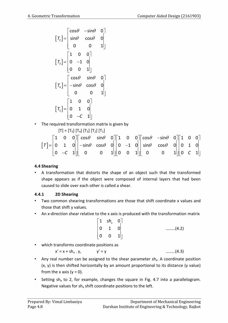
4. Geometric Transformation Computer Aided Design (2161903)
Prepared By: Vimal Limbasiya Department of Mechanical Engineering Page 4.8 Darshan Institute of Engineering & Technology, Rajkot
2
cos sin 0
sin cos 0
0 0 1
T
3
1 0 0
0 1 0
0 0 1
T
4
cos sin 0
sin cos 0
0 0 1
T
5
1 0 0
0 1 0
0 1
T
C
• The required transformation matrix is given by
[T] = [T5] [T4] [T3] [T2] [T1]
1 0 0 cos sin 0 1 0 0 cos sin 0 1 0 0
0 1 0 sin cos 0 0 1 0 sin cos 0 0 1 0
0 1 0 0 1 0 0 1 0 0 1 0 1
T
C C
4.4 Shearing
• A transformation that distorts the shape of an object such that the transformed
shape appears as if the object were composed of internal layers that had been
caused to slide over each other is called a shear.
4.4.1 2D Shearing
• Two common shearing transformations are those that shift coordinate x values and
those that shift y values.
• An x-direction shear relative to the x axis is produced with the transformation matrix
1 0
0 1 0
0 0 1
xsh
………(4.2)
• which transforms coordinate positions as
x’ = x + shx . y, y’ = y ………(4.3)
• Any real number can be assigned to the shear parameter shx. A coordinate position
(x, y) is then shifted horizontally by an amount proportional to its distance (y value)
from the x axis (y = 0).
• Setting shx to 2, for example, changes the square in Fig. 4.7 into a parallelogram.
Negative values for shx shift coordinate positions to the left.

Computer Aided Design (2161903) 4. Geometric Transformation
Department of Mechanical Engineering Prepared By: Vimal Limbasiya Darshan Institute of Engineering & Technology, Rajkot Page 4.9
Fig. 4.7 A unit square (a) is converted to a parallelogram (b) using the x direction shear
matrix 4.2 with shx = 2.
• We can generate x-direction shears relative to other reference lines with
1
0 1 0
0 0 1
x x refsh sh y
……..(4.4)
• with coordinate positions transformed as
x’ = x + shx (y – yref), y’ = y ……..(4.5)
• An example of this shearing transformation is given in Fig.4.8 for a shear parameter
value of 1 /2 relative to the line yref = –1.
Fig. 4.8 A unit square (a) is transformed to a shifted parallelogram (b)
with shx = 1/2 and yref = –1 in the shear matrix 4.4.
• A y-direction shear relative to line x = xref is generated with transformation matrix
1 0 0
1
0 0 1y y refsh sh x
…….(4.6)
• which generates transformed coordinate positions
x’ = x, y’ = y + shy (x – xref) ………(4.7)

4. Geometric Transformation Computer Aided Design (2161903)
Prepared By: Vimal Limbasiya Department of Mechanical Engineering Page 4.10 Darshan Institute of Engineering & Technology, Rajkot
Fig. 4.9 A unit square (a) is turned into a shifted parallelogram (b) with parameter values shy
= 1/2 and xref = –1 in the y direction using shearing transformation 4.6.
• This transformation shifts a coordinate position vertically by an amount proportional
to its distance from the reference line x = xref. Fig. 4.9 illustrates the conversion of a
square into a parallelogram with shy = 1/2 and xref = –1.
• Shearing operations can be expressed as sequences of basic transformations. The x-
direction shear matrix 4.2, for example, can be written as a composite
transformation involving a series of rotation and scaling matrices that would scale
the unit square of Fig. 4.9 along its diagonal, while maintaining the original lengths
and orientations of edges parallel to the x axis.
• Shifts in the positions of objects relative to shearing reference lines are equivalent to
translations.
4.4.2 3D Shearing
• In two dimensions, transformations relative to the x or y axes to produce distortions
in the shapes of objects. In three dimensions, we can also generate shears relative to
the z axis.
Fig 4.10
• As an example of three-dimensional shearing, the following transformation produces
a z-axis shear:
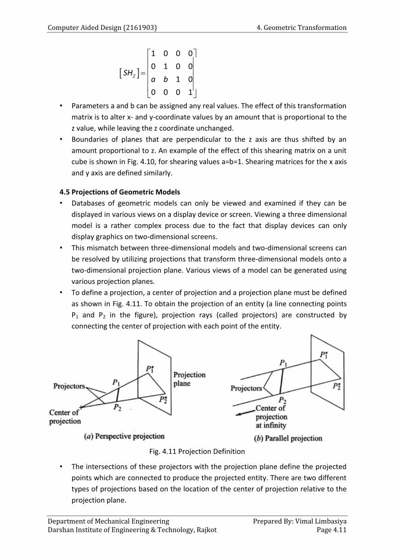
Computer Aided Design (2161903) 4. Geometric Transformation
Department of Mechanical Engineering Prepared By: Vimal Limbasiya Darshan Institute of Engineering & Technology, Rajkot Page 4.11
1 0 0 0
0 1 0 0
1 0
0 0 0 1
ZSHa b
• Parameters a and b can be assigned any real values. The effect of this transformation
matrix is to alter x- and y-coordinate values by an amount that is proportional to the
z value, while leaving the z coordinate unchanged.
• Boundaries of planes that are perpendicular to the z axis are thus shifted by an
amount proportional to z. An example of the effect of this shearing matrix on a unit
cube is shown in Fig. 4.10, for shearing values a=b=1. Shearing matrices for the x axis
and y axis are defined similarly.
4.5 Projections of Geometric Models
• Databases of geometric models can only be viewed and examined if they can be
displayed in various views on a display device or screen. Viewing a three dimensional
model is a rather complex process due to the fact that display devices can only
display graphics on two-dimensional screens.
• This mismatch between three-dimensional models and two-dimensional screens can
be resolved by utilizing projections that transform three-dimensional models onto a
two-dimensional projection plane. Various views of a model can be generated using
various projection planes.
• To define a projection, a center of projection and a projection plane must be defined
as shown in Fig. 4.11. To obtain the projection of an entity (a line connecting points
P1 and P2 in the figure), projection rays (called projectors) are constructed by
connecting the center of projection with each point of the entity.
Fig. 4.11 Projection Definition
• The intersections of these projectors with the projection plane define the projected
points which are connected to produce the projected entity. There are two different
types of projections based on the location of the center of projection relative to the
projection plane.

4. Geometric Transformation Computer Aided Design (2161903)
Prepared By: Vimal Limbasiya Department of Mechanical Engineering Page 4.12 Darshan Institute of Engineering & Technology, Rajkot
• If the center is at a finite distance from the plane, perspective projection results and
all the projectors meet at the center. If, on the other hand, the center is at an infinite
distance, all the projectors become parallel (meet at infinity) and parallel projection
results. Perspective projection is usually a part of perspective, or projective,
geometry.
• Such geometry does not preserve parallelism, that is, no two lines are parallel.
Parallel projection is a part of affine geometry which is identical to Euclidean
geometry. In affine geometry, parallelism is an important concept and therefore is
preserved.
4.5.1. Perspective projection
• Perspective projection creates an artistic effect that adds some realism to
perspective views. As can be seen from Fig. 4.11(a), the size of an entity is inversely
proportional to its distance from the center of projection; that is, the closer the
entity to the center, the larger its size is.
• Perspective views are not popular among engineers and draftsmen because actual
dimensions and angles of objects and therefore shapes, cannot be preserved, which
implies that measurements cannot be taken from perspective views directly. In
addition, perspective projection does not preserve parallelism.
• In order to define perspective projection, a centre of projection and a projection
plane are required. The centre of projection is placed along the z-axis and the image
is projected onto z = 0 or xy plane.
• The transformation of perspective projection is given by:
P* = Po P
where
1 0 0 0
0 1 0 0
0 0 0 0
0 0 1 / 1
OP
d
P is the given point.
P* is the reflected point.
d is the distance between the centre of projection to the projection plane.
4.5.2. Orthographic Projection
• Unlike perspective projection, parallel projection preserves actual dimensions and
shapes of objects. It also preserves parallelism. Angles are preserved only on faces of
the object which are parallel to the projection plane.
• There are two types of parallel projections based on the relation between the
direction of projection and the projection plane. If this direction is normal to the
projection plane, orthographic projection and views result.

Computer Aided Design (2161903) 4. Geometric Transformation
Department of Mechanical Engineering Prepared By: Vimal Limbasiya Darshan Institute of Engineering & Technology, Rajkot Page 4.13
• The orthographic projection system is to include a total of six projecting planes in
any direction required for complete description.
• A typical example is shown in Fig. 4.12 where the object is enclosed in a box such
that there are 6 mutually perpendicular projecting planes on which all possible 6
views of the object can be projected.
• This would help in obtaining all the details of the object as shown in Fig. 4.13. The
visible lines are shown with the help of continuous lines while those that are not
visible are shown by means of broken lines.
Fig. 4.12 An object Enclosed in a Cube for Obtaining Various Parallel Projections
• Obtaining the orthographic projections is relatively straight forward because of the
parallel projections involved. The top view can be obtained by setting z = 0. The
transformation matrix will then be
1 0 0 0
0 1 0 0
0 0 0 0
0 0 0 1
TOPM
• For obtaining the front view, y = 0 and then the resulting coordinates (x, z) will be
rotated by 900 such that the Z axis coincides with the Y axis. The transformation
matrix will then be
1 0 0 0
0 0 1 0
0 0 0 0
0 0 0 1
FRONTM

4. Geometric Transformation Computer Aided Design (2161903)
Prepared By: Vimal Limbasiya Department of Mechanical Engineering Page 4.14 Darshan Institute of Engineering & Technology, Rajkot
Fig. 4.13 Orthographic Projection of an Object.
• Similarly for obtaining the right side view, x = 0 and then the coordinate system is
rotated such that Y axis coincides with the X axis and the Z axis coincides with the Y
axis. The transformation matrix will then be
0 0 1 0
0 1 0 0
0 0 0 0
0 0 0 1
RIGHTM
4.6 Window to View-port transformation
• A world-coordinate area selected for display is called a window. An area on a display
device to which a window is mapped is called a viewport. The window defines what
is to be viewed; the viewport defines where it is to be displayed.
• Often, windows and viewports are rectangles in standard position, with the
rectangle edges parallel to the coordinate axes. Other window or viewport
geometries, such as general polygon shapes and circles, are used in some
applications, but these shapes take longer to process.
Fig. 4.14 A viewing transformation using standard rectangles for the window and viewport

Computer Aided Design (2161903) 4. Geometric Transformation
Department of Mechanical Engineering Prepared By: Vimal Limbasiya Darshan Institute of Engineering & Technology, Rajkot Page 4.15
• In general, the mapping of a part of a world-coordinate scene to device coordinates
is referred to as a viewing transformation. Sometimes the two-dimensional viewing
transformation is simply referred to as the window-to-viewport transformation or
the windowing transformation.
• Fig. 4.14 illustrates the mapping of a picture section that falls within a rectangular
window onto a designated rectangular viewport.
• Fig. 4.15 illustrates the window-to-viewport mapping. A point at position (xw, yw) in
the window is mapped into position (xv,yv) in the associated viewport. To maintain
the same relative placement in the viewport as in the window, we require that
min min
max min max min
xv xv xw xw
xv xv xw xw
min min
max min max min
yv yv yw yw
yv yv yw yw
………………(4.8)
Solving these expressions for the viewport position (xv, yv), we have
min min
min min
xv xv (xw xw )sx
yv yv (yw yw )sy
………………(4.9)
Where the scaling factors are
max min
max min
max min
max min
xv xvsx
xw xw
yv yvsy
yw yw
……………….(4.10)
Eq. 4.9 can also be derived with a set of transformations that converts the window
area into the viewport area. This conversion is performed with the following
sequence of transformations:
Fig. 4.15 A point at position (xw, yw) in a designated window is mapped to viewport
coordinates (xv,yv) so that relative positions in the two areas are the same.
1. Perform a scaling transformation using a fixed-point position of (xwmin, ywmin) that
scales the window area to the size of the viewport.
2. Translate the scaled window area to the position of the viewport.

4. Geometric Transformation Computer Aided Design (2161903)
Prepared By: Vimal Limbasiya Department of Mechanical Engineering Page 4.16 Darshan Institute of Engineering & Technology, Rajkot
• Relative proportions of objects are maintained if the scaling factors are the same
(sx = sy). Otherwise, world objects will be stretched or contracted in either the x or y
direction when displayed on the output device.
• Character strings can be handled in two ways when they are mapped to a viewport.
The simplest mapping maintains a constant character size, even though the viewport
area may be enlarged or reduced relative to the window.
• This method would be employed when text is formed with standard character fonts
that cannot be changed. In systems that allow for changes in character size, string
definitions can be windowed the same as other primitives. For characters formed
with line segments, the mapping to the viewport can be carried out as a sequence of
line transformations.
• From normalized coordinates, object descriptions are mapped to the various display
devices. Any number of output devices can be open in a particular application, and
another window-to-viewport transformation can be performed for each open output
device.
• This mapping, called the workstation transformation, is accomplished by selecting a
window area in normalized space and a viewport area in the coordinates of the
display device.
• With the workstation transformation, we gain some additional control over the
positioning of a scene on individual output devices. As illustrated in Fig. 4.16, we can
use workstation transformations to partition a view so that different parts of
normalized space can be displayed on different output devices.
Fig. 4.16 Mapping selected parts of a scene in normalized coordinates to different video
monitors with workstation transformations.

Computer Aided Design (2161903) 4. Geometric Transformation
Department of Mechanical Engineering Prepared By: Vimal Limbasiya Darshan Institute of Engineering & Technology, Rajkot Page 4.17
Example 4.1
A triangle ABC with vertices A (32, 22), B (88, 20) and C (32, 82) is to be scaled by a factor
of 0.6 about a point X (50, 42). Determine the co-ordinates of the vertices for the scaled
triangle.
Solution:
Data given:
Sx = Sy = 0.6
Scaling about a point X (50, 42)
So, first translate the object to origin then scale the object and then translate back the
scaled object to the given point X (50, 42). ' ' ' 1ABC ABC T S T
' ' '
32 22 1 1 0 0 0.6 0 0 1 0 0
88 20 1 0 1 0 0 0.6 0 0 1 0
32 82 1 50 42 1 0 0 1 50 42 1
A BC
' ' '
32 22 1 1 0 0 0.6 0 0
88 20 1 0 1 0 0 0.6 0
32 82 1 50 42 1 50 42 1
A BC
' ' '
32 22 1 0.6 0 0
88 20 1 0 0.6 0
32 82 1 20 16.8 1
A BC
' ' '
39.2 30 1
72.8 28.8 1
39.2 66 1
A BC
Answer: New vertices are A’ (39.2, 30), B’ (72.8, 28.8) and C’ (39.2, 66).
Example 4.2
Using transformation matrix, determine the new co-ordinates of triangle ABC with
vertices A (0, 0), B (3, 2) and C (2, 3) after it is rotated by 45° clockwise about origin.
Solution:
Data given:

4. Geometric Transformation Computer Aided Design (2161903)
Prepared By: Vimal Limbasiya Department of Mechanical Engineering Page 4.18 Darshan Institute of Engineering & Technology, Rajkot
Rotation about origin 45° clockwise
Hence, θ = -45° ' ' 'ABC ABC R
' ' '
0 0 1 ( 45 ) ( 45 ) 0
3 2 1 ( 45 ) ( 45 ) 0
2 3 1 0 0 1
Cos Sin
A BC Sin Cos
' ' '
0 0 1 0.707 0.707 0
3 2 1 0.707 0.707 0
2 3 1 0 0 1
A BC
' ' '
0 0 0
3.536 0.707 0
3.536 0.707 1
A BC
Answer: New vertices are A’ (0, 0), B’ (3.536, -0.707) and C’ (3.536, 0.707).
Example 4.3
A rectangle ABCD has vertices A (1, 1), B (2, 1), C (2, 3) and D (1, 3). It has to be rotated by
30° counter clockwise about a point P (3, 2). Determine the new co-ordinates of the
vertices for the rectangle.
Solution:
Data given:
Rotation about a point 45° counter clockwise
Hence, θ = 45°
Rotation about a point P (3, 2), so, first translate the object to origin then rotate the object
and then translate back the rotated object to the given point P (3, 2). ' ' ' ' 1ABC D ABCD T R T
' ' ' '
1 1 11 0 0 30 30 0 1 0 0
2 1 10 1 0 30 30 0 0 1 0
2 3 13 2 1 0 0 1 3 2 1
1 3 1
Cos Sin
A BC D Sin Cos
' ' ' '
1 1 11 0 0 0.866 0.5 0 1 0 0
2 1 10 1 0 0.5 0.866 0 0 1 0
2 3 13 2 1 0 0 1 3 2 1
1 3 1
A BC D
' ' ' '
1 1 11 0 0 0.866 0.5 0
2 1 10 1 0 0.5 0.866 0
2 3 13 2 1 3 2 1
1 3 1
A BC D

Computer Aided Design (2161903) 4. Geometric Transformation
Department of Mechanical Engineering Prepared By: Vimal Limbasiya Darshan Institute of Engineering & Technology, Rajkot Page 4.19
' ' ' '
1 1 10.866 0.5 0
2 1 10.5 0.866 0
2 3 11.402 1.232 1
1 3 1
A BC D
' ' ' '
1.768 0.134 1
2.634 0.634 1
1.634 2.366 1
0.768 1.866 1
A B C D
Answer: New vertices are A’ (1.768, 0.134), B’ (2.634, 0.634), C’ (1.634, 2.366) and D’ (0.768,
1.866).
Example 4.4
A triangle ABC with vertices at A (0, 0), B (4, 0) and C (2, 3) is given. Perform the following
operations for it.
(i) Translation through 4 and 2 units along X and Y direction respectively,
(ii) Rotation through 90° in counter clockwise direction about the new position of
point C.
Solution:
(i) Translation by tx = 4 and ty = 2. ' ' 'ABC ABC T
' ' '
0 0 1 1 0 0
4 0 1 0 1 0
2 3 1 1x y
A BC
t t
' ' '
0 0 1 1 0 0
4 0 1 0 1 0
2 3 1 4 2 1
A BC

4. Geometric Transformation Computer Aided Design (2161903)
Prepared By: Vimal Limbasiya Department of Mechanical Engineering Page 4.20 Darshan Institute of Engineering & Technology, Rajkot
' ' '
4 2 1
8 2 1
6 5 1
A B C
Answer: New vertices are A’ (4, 2), B’ (8, 2) and C’ (6, 5).
(ii) Rotation about the new point C’ (6, 5) through 90° counter-clockwise.
Hence, θ = 90°
Rotation about a point C’ (6, 5), so, first translate the object to origin then rotate the
object and then translate back the rotated object to the given point C’ (6, 5). '' '' '' ' ' ' 1A B C ABC T R T
'' '' ''
4 2 1 1 0 0 90 90 0 1 0 0
8 2 1 0 1 0 90 90 0 0 1 0
6 5 1 6 5 1 0 0 1 6 5 1
Cos Sin
A B C Sin Cos
'' '' ''
4 2 1 1 0 0 0 1 0 1 0 0
8 2 1 0 1 0 1 0 0 0 1 0
6 5 1 6 5 1 0 0 1 6 5 1
A B C
'' '' ''
4 2 1 1 0 0 0 1 0
8 2 1 0 1 0 1 0 0
6 5 1 6 5 1 6 5 1
A B C
'' '' ''
4 2 1 0 1 0
8 2 1 1 0 0
6 5 1 11 1 1
A B C
'' '' ''
9 3 1
9 7 1
6 5 1
A B C
Answer: New vertices are A’’ (9, 3), B’’ (9, 7) and C’’ (6, 5).

Computer Aided Design (2161903) 4. Geometric Transformation
Department of Mechanical Engineering Prepared By: Vimal Limbasiya Darshan Institute of Engineering & Technology, Rajkot Page 4.21
Example 4.5
The co-ordinates of three vertices of the triangle are P (50, 20), Q (110, 20) and R (80, 60).
Determine the co-ordinates of the vertices for the new reflected triangle if it is to be
reflected about:
(i) x-axis,
(ii) Line y = x.
Solution:
(i) Reflection about x-axis ' ' '
xP QR PQR M
' ' '
50 20 1 1 0 0
110 20 1 0 1 0
80 60 1 0 0 1
P Q R
' ' '
50 20 1
110 20 1
80 60 1
P Q R
Answer: New vertices are P’ (50, -20), Q’ (110, -20) and R’ (80, -60).
(ii) Reflection about line y = x ' ' '
( )y xP QR PQR M
' ' '
50 20 1 0 1 0
110 20 1 1 0 0
80 60 1 0 0 1
P Q R
' ' '
20 50 1
20 110 1
60 80 1
P Q R
Answer: New vertices are P’ (20, 50), Q’ (20, 110) and R’ (60, 80).
Example 4.6
Reflect the diamond shape polygon whose vertices are A (-2, 0), B (0, -1) C (2, 0) and D (0,
1) about an arbitrary line L which is represented by equation y = 0.5 x + 1.
Solution:
Data given:
Reflect the polygon about line y = 0.5 x + 1
So, first translate the object to origin, and then rotate the object such that the line coincides
with x-axis, then reflect the polygon about x-axis, then rotate back and then translate back.
y = 0.5 x + 1
0.5 tanm 1tan 0.5 26.565 (Clockwise)
26.565
Also, when x = 0, y = 1 and when y = 0, x = -2.

4. Geometric Transformation Computer Aided Design (2161903)
Prepared By: Vimal Limbasiya Department of Mechanical Engineering Page 4.22 Darshan Institute of Engineering & Technology, Rajkot
2, 0x yt t
' ' ' ' 1 1ABC D ABCD T R M R T
2 0 11 0 0 0 1 0 0 ( ) ( ) 0 1 0 0
0 1 10 1 0 0 0 1 0 ( ) ( ) 0 0 1 0
2 0 11 0 0 1 0 0 1 0 0 1 1
0 1 1 x y x y
Cos Sin Cos Sin
Sin Cos Sin Cos
t t t t
2 0 11 0 0 ( 26.565 ) ( 26.565 ) 0 1 0 0 26.565 26.565 0 1 0 0
0 1 10 1 0 ( 26.565 ) ( 26.565 ) 0 0 1 0 26.565 26.565 0 0 1 0
2 0 12 0 1 0 0 1 0 0 1 0 0 1 2 0 1
0 1 1
Cos Sin Cos Sin
Sin Cos Sin Cos
2 0 11 0 0 0.8944 0.4472 0 1 0 0 0.8944 0.4472 0 1 0 0
0 1 10 1 0 0.4472 0.8944 0 0 1 0 0.4472 0.8944 0 0 1 0
2 0 12 0 1 0 0 1 0 0 1 0 0 1 2 0 1
0 1 1
2 0 11 0 0 0.8944 0.4472 0 1 0 0 0.8944 0.4472 0
0 1 10 1 0 0.4472 0.8944 0 0 1 0 0.4472 0.8944 0
2 0 12 0 1 0 0 1 0 0 1 2 0 1
0 1 1
2 0 11 0 0 0.8944 0.4472 0 0.8944 0.4472 0
0 1 10 1 0 0.4472 0.8944 0 0.4472 0.8944 0
2 0 12 0 1 0 0 1 2 0 1
0 1 1
2 0 11 0 0 0.6 0.8 0
0 1 10 1 0 0.8 0.6 0
2 0 12 0 1 2 0 1
0 1 1
2 0 10.6 0.8 0
0 1 10.8 0.6 0
2 0 10.8 1.6 1
0 1 1
2 0 1
1.6 2.2 1
0.4 3.2 1
0 1 1
Answer: New vertices are A’ (-2, 0), B’ (-1.6, 2.2), C’ (0.4, 3.2) and D’ (0, 1).

Department of Mechanical Engineering Prepared By: A.J.Makadia Darshan Institute of Engineering & Technology, Rajkot Page 5.1
5 FINITE ELEMENT ANALYSIS
Course Contents
5.1 Basic Concept
5.2 Historical Background
5.3 Definition
5.4 Engineering Applications of
the Finite Element Method
5.5 General procedure of Finite
Element Method
5.6 Stress analysis of stepped bar
5.7 Penalty Approach
5.8 Effect of Temperature on
Elements
5.9 Discretization of the Domain
5.10 Discretization Process
5.11 Automatic Mesh Generation
5.12 Analysis of Trusses
5.13 Principle of Minimum
Potential Energy
5.14 Natural OR Intrinsic
Coordinate System
5.15 Shape function in Natural
Coordinate System

5. Finite Element Analysis Computer Aided Design (2161903)
Prepared By: VimalLimbasiya Department of Mechanical Engineering Page 5.2 Darshan Institute of Engineering & Technology, Rajkot
5.1 Basic Concept
The basic idea in the finite element method is to find the solution of a complicated
problem by replacing it by a simpler one.
Since the actual problem is replaced by a simpler one in finding the solution, we will
be able to find only an approximate solution rather than the exact solution.
The existing mathematical tools will not be sufficient to find the exact solution (and
sometimes, even an approximate solution) of most of the practical problems.
Thus, in the absence of any other convenient method to find even the approximate
solution of a given problem, we have to prefer the finite element method.
Moreover, in the finite element method, it will often be possible to improve or refine
the approximate solution by spending more computational effort.
In the finite element method, the solution region is considered as built up of many
small, interconnected sub regions called finite elements. As an example of how a
finite element model might be used to represent a complex geometrical shape,
consider the milling machine structure shown in Figure 5.1(a).
Since it is very difficult to find the exact response (like stresses and displacements) of
the machine under any specified cutting (loading) condition, this structure is
approximated as composed of several pieces as shown in Figure 5.1(b) in the finite
element method. In each piece or element, a convenient approximate solution is
assumed and the conditions of overall equilibrium of the structure are derived. The
satisfaction of these conditions will yield an approximate solution for the
displacements and stresses.
Fig. 5.1 Representation of a Milling Machine Structure by Finite Elements.

Computer Aided Design (2161903) 5. Finite Element Analysis
Department of Mechanical Engineering Prepared By: VimalLimbasiya Darshan Institute of Engineering & Technology, Rajkot Page 5.3
Figure 5.2 shows the finite element idealization of a fighter aircraft.
Fig. 5.2Finite Element Mesh of aFighter Aircraft.
5.2 Historical Background
Although the name of the finite element method was given recently, the concept dates
back for several centuries. For example, ancient mathematicians found the
circumference of a circle by approximating it by the perimeter of a polygon as shown
in Figure 5.3.
In terms of the present day notation, each side of the polygon can be called a “finite
element.” By considering the approximating polygon inscribed or circumscribed, one
can obtain a lower bound S(l)
or an upper bound S(u)
for the true circumference S.
Fig. 5.3 Lower and Upper Bounds to the Circumference of a Circle.

5. Finite Element Analysis Computer Aided Design (2161903)
Prepared By: VimalLimbasiya Department of Mechanical Engineering Page 5.4 Darshan Institute of Engineering & Technology, Rajkot
Furthermore, as the number of sides of the polygon is increased, the approximate
values converge to the true value. These characteristics, as will be seen later, will hold
true in any general finite element application.
To find the differential equation of a surface of minimum area bounded by a specified
closed curve, Schellback discretized the surface into several triangles and used a finite
difference expression to find the total discretized area in 1851.
In the current finite element method, a differential equation is solved by replacing it
by a set of algebraic equations. Since the early 1900s, the behavior of structural
frameworks, composed of several bars arranged in a regular pattern, has been
approximated by that of an isotropic elastic body.
In 1943, Courant presented a method of determining the torsional rigidity of a hollow
shaft by dividing the cross section into several triangles and using a linear variation of
the stress function ϕ over each triangle in terms of the values of ϕ at net points (called
nodes in the present day finite element terminology).
This work is considered by some to be the origin of the present-day finite element
method. Since mid-1950s, engineers in aircraft industry have worked on developing
approximate methods for the prediction of stresses induced in aircraft wings.
In 1956, Turner, Cough, Martin, and Topp presented a method for modeling the wing
skin using three-node triangles. At about the same time, Argyris and Kelsey presented
several papers outlining matrix procedures, which contained some of the finite
element ideas, for the solution of structural analysis problems. Reference is
considered as one of the key contributions in the development of the finite element
method.
The name finite element was coined, for the first time, by Clough in 1960. Although
the finite element method was originally developed mostly based on intuition and
physical argument, the method was recognized as a form of the classical Rayleigh-
Ritz method in the early 1960s.
Once the mathematical basis of the method was recognized, the developments of new
finite elements for different types of problems and the popularity of the method
started to grow almost exponentially.
The digital computer provided a rapid means of performing the many calculations
involved in the finite element analysis and made the method practically viable. Along
with the development of high-speed digital computers, the application of the finite
element method also progressed at a very impressive rate.
Zienkiewicz and Cheung presented the broad interpretation of the method and its
applicability to any general field problem. The book by Przemienieckipresents the
finite element method as applied to the solution of stress analysis problems.
5.3 Definition:
In Finite Element Analysis, the structure or body is divided into finite numbers of
elements, the solution is obtained for individual element and solution of all elements
is assembled to give distribution of field variable over entire region.

Computer Aided Design (2161903) 5. Finite Element Analysis
Department of Mechanical Engineering Prepared By: VimalLimbasiya Darshan Institute of Engineering & Technology, Rajkot Page 5.5
For example: Heat Analysis Field variable is Temperature
Stress & strain Field variable is Displacement.
5.4 Engineering Applications of the Finite Element Method
The finite element method was developed originally for the analysis of aircraft structures.
I. Equilibrium problems or steady-state or time-independent problems
In an equilibrium problem, we need to find the steady-state displacement or stress
distribution if it is a solid mechanics problem,
Temperature or heat flux distribution if it is a heat transfer problem and
Pressure or velocity distribution if it is a fluid mechanics problem.
II. Eigenvalue problems
In eigenvalue problems also, time will not appear explicitly. They may be
considered as extensions of equilibrium problems in which critical values of
certain parameters are to be determined in addition to the corresponding steady-
state configurations.
In these problems, we need to find the natural frequencies or buckling loads and
mode shapes if it is a solid mechanics or structures problem.
Stability of laminar flows if it is a fluid mechanics problem and
Resonance characteristics if it is an electrical circuit problem.
III. Propagation or transient problems
The propagation or transient problems are time-dependent problems. This type of
problemarises, for example, whenever we are interested in finding the response of
a body undertime-varying force in the area of a solid mechanics
Under sudden heating or cooling inthe field of heat transfer.
Crack propagation.
Engineering Applications of the Finite Element Method
Area of Study Equilibrium Problems Eigenvalue
Problems Propagation Problems
1.Civil
engineering
structures
Static analysis of
trusses, frames,folded
plates, shell roofs,
shearwalls, bridges,
andprestressedconcrete
structures
Natural frequencies
andmodes of
structures;stability of
structures
Propagation of stress
waves;response of
structures toaperiodic
loads
2. Aircraft
structures
Static analysis of
aircraft wings,
fuselages, fins, rockets,
spacecraft, and missile
structures
Natural frequencies,
flutter, and stability
of
aircraft,
rocket,spacecraft,
and missilestructures
Response of aircraft
structures torandom
loads; dynamic
responseof aircraft and
spacecraft toaperiodic
loads

5. Finite Element Analysis Computer Aided Design (2161903)
Prepared By: VimalLimbasiya Department of Mechanical Engineering Page 5.6 Darshan Institute of Engineering & Technology, Rajkot
3. Heat
conduction
Steady-state
temperature
distribution in solids
and fluids
–
Transient heat flow in
rocketnozzles, internal
combustionengines,
turbineblades, fins, and
building structures
4. Geomechanics Analysis of excavations,
retainingwalls,undergro
und openings,rock
joints, and soil–structureinteraction
problem; stressanalysis
in soils, dams,
layeredpiles, and
machinefoundations
Natural frequencies
andmodes of dam-
reservoirsystems and
soil–structure
interactionproblems
Time-dependent soil–structureinteraction
problems;
transientseepage in soils
and rocks;stress wave
propagation in soils
and rocks
5. Hydraulic
andwater
resourcesengineeri
ng;hydrodynamics
Analysis of potential
flows, freesurface flows,
boundary layer
flows, viscous flows,
transonicaerodynamic
problems; analysisof
hydraulic structures and
dams
Natural periods
andmodes of
shallowbasins, lakes,
andharbors; sloshing
ofliquids in rigid
andflexible
containers
Analysis of unsteady
fluid flowand wave
propagation problems;
transient seepage in
aquifers andporous
media; rarefied
gasdynamics;magnetohyd
rodynamicflows
6. Nuclear
engineering
Analysis of nuclear
pressurevessels and
containmentstructures;
steady –
stateTemperaturedistrib
ution in reactor
components
Natural frequencies
andstability of
containmentstructure
s; neutron
fluxdistribution
Response of reactor
containmentstructures to
dynamic loads;unsteady
temperature distributionin
reactor components;
thermaland viscoelastic
analysis ofreactor
structures
7. Biomedical
engineering
Stress analysis of
eyeballs, bones,and
teeth; load-bearing
capacityof implant and
prosthetic
systems;mechanics of
heart valves
–
Impact analysis of
skull;dynamics of
anatomicalstructures
8. Mechanical
Design
Stress concentration
problems;stress analysis
of pressurevessels,
pistons,
compositematerials,
linkages, and gears
Natural frequencies
andstability of
linkages,gears, and
machinetools
Crack and fracture
problemsunder dynamic
loads
9.
Electricalmachine
s
andelectromagneti
cs
Steady-state analysis
ofsynchronous and
inductionmachines,
eddy current, andcore
losses in electric
machines,magnetostatic
s
–
Transient behavior
ofElectromechanicaldevic
es suchas motors and
actuators,magnetodynami
cs

Computer Aided Design (2161903) 5. Finite Element Analysis
Department of Mechanical Engineering Prepared By: VimalLimbasiya Darshan Institute of Engineering & Technology, Rajkot Page 5.7
5.5 General procedure of Finite Element Method
Step 1: Divide structure into discrete elements (discretization).
Divide the structure or solution region into subdivisions or elements. Hence, the
structure is to be modeled with suitable finite elements.
The number, type, size, and arrangement of the elements are to be decided.
Step 2: Select a proper interpolation or displacement model.
Since the displacement solution of a complex structure under any specified
loadconditions cannot be predicted exactly, we assume some suitable solution within
anelement to approximate the unknown solution. The assumed solution must besimple
from a computational standpoint, but it should satisfy certain
convergencerequirements.
In general, the solution or the interpolation model is taken in the formof a polynomial.
Step 3: Derive element stiffness matrices and load vectors.
From the assumed displacement model finding,
Stiffness matrix – [K]e
Load vector. – [P]e
Step 4: Assemble element equations to obtain the overall equilibrium equations.
Since the structure is composed of several finite elements, the individual element
stiffness matrices and load vectors are to be assembled in a suitable manner and the
overall equilibrium equations have to be formulated as
[K] [ϕ] = [P]
Where [K] = the assembled stiffness matrix
[ϕ] = the vector of nodal displacements
[P] = Load vector
Step 5: Solve for the unknown nodal displacements.
The overall equilibrium equations have to be modified to account for the boundaryconditions
of the problem. After the incorporation of the boundary conditions, theequilibrium equations
can be expressed as
[K] [ϕ] = [P]
Step 6: Compute element strains and stresses.
From the known nodal displacementsϕ, if required, the element strains and stressescan be
computed by using the necessary equations of solid or structural mechanics.
5.6 Stress analysis of stepped bar

5. Finite Element Analysis Computer Aided Design (2161903)
Prepared By: VimalLimbasiya Department of Mechanical Engineering Page 5.8 Darshan Institute of Engineering & Technology, Rajkot
Fig. 5.4 Steeped bar under Axial load
Step 1: Idealization.
The bar is idealized as an assemblage of two elements, one element for each step of the bar
asshown in Figure 5.4(b). Each element is assumed to have nodes at the ends so that the
stepped barwill have a total of three nodes.
Since the load is applied in the axial direction, the axialdisplacements of the three nodes are
considered as the nodal unknown degrees of freedom of thesystem, and are denoted as Φ1,Φ2,
and Φ3 as shown in Figure 5.4(b).
Step 2: Develop interpolation or displacement model.
Since the two end displacements of element e, Φ1(e)
, and Φ2(e)
, are considered the degrees of
freedom, the axial displacement, ϕ(x), within the element e is assumed to vary linearly as
(Figure 5.4(c)): ϕ(x) = a+bx (E.1)
Step 3: Derive element stiffness matrix and element load vector.

Computer Aided Design (2161903) 5. Finite Element Analysis
Department of Mechanical Engineering Prepared By: VimalLimbasiya Darshan Institute of Engineering & Technology, Rajkot Page 5.9
The element stiffness matrices can be derived from the principle of minimum potential
energy. Forthis, we write the potential energy of the bar (I) under axial deformation as
I = strain energy – work done by external forces
= (1)
+ (2)
– Wp
where(e)
represents the strain energy of element e, and Wp denotes the work done by
external forcesacting on the bar.
Apply principle of potential energy
Since there are only concentrated loads acting at the nodes of the bar (and no distributed load
actson the bar), the work done by external forces can be expressed as
Wp = Φ1P1 +Φ2P2 +Φ3P3
In the present case, Φ1 = 0 since node 1 is fixed while the loadsapplied externally at the nodes
1, 2, and 3 in the directions of Φ1, Φ2, and Φ3, respectively, areP1 = unknown (denotes the
reaction at the fixed node 1 where the displacement Φ1 is zero),P2 = 0, and P3 = 1 N.
If the bar as a whole is in equilibrium under the loads,
1
2
3
P
P P
P
the principle of
minimumpotential energy gives

5. Finite Element Analysis Computer Aided Design (2161903)
Prepared By: VimalLimbasiya Department of Mechanical Engineering Page 5.10 Darshan Institute of Engineering & Technology, Rajkot
Step 4: Assemble element stiffness matrices and element load vectors
This step includes the assembly of element stiffness matrices [K]e and element load vectors
[P]e toobtain the overall or global equilibrium equations.
[K] [ϕ] = [P]
where[K] is the assembled or global stiffness matrix =
2( )
1
[K ]e
e
1
2
3
= vector ofglobal displacements.
Example 5.1:A1 = 200 mm2, E1 = E2 = E = 2 x 10
6 N/mm
2
A2 = 100 mm2, l1 = l2 = 100 mm
P3 = 1000 N. Find: Displacement and stress & strain.
Let overall stiffness matrix [K] = [K(1)
] + [K(2)
]

Computer Aided Design (2161903) 5. Finite Element Analysis
Department of Mechanical Engineering Prepared By: VimalLimbasiya Darshan Institute of Engineering & Technology, Rajkot Page 5.11
In the present case, external loads act only at the node points; as such, there is no need to
assemblethe element load vectors. The overall or global load vector can be written as
By solving the matrix
Φ2 = 0.25 × 10⁻⁶cm and
Φ3 = 0.75 × 10⁻⁶cm
Derive element strains and stresses.
Once the displacements are computed, the strains in the elements can be found as
The stresses in the elements are given by
Example 5.2:A thin plate as shown in Fig. 5.5(a) has uniform thickness of 2 cm and its
modulus of elasticity is 200 x 103 N/mm
2 and density 7800 kg/m
3. In addition to its self
weight the plate is subjected to a point load P of500 N is applied at its midpoint.
Solve the following:
(i) Finite element model with two finite elements.
(ii) Global stiffness matrix.
(iii) Global load matrix.
(iv) Displacement at nodal point.

5. Finite Element Analysis Computer Aided Design (2161903)
Prepared By: VimalLimbasiya Department of Mechanical Engineering Page 5.12 Darshan Institute of Engineering & Technology, Rajkot
(v) Stresses in each element.
(vi) Reaction at support.
(a) Fig. 5.5 (b)
(i) The tapered plate can be idealized as two element model with the tapered area
converted to the rectangular equivalent area Refer Fig. (b). The areas A1 and A2
are equivalent areas calculated as
2
1
15 11.252 26.25
2A cm
2
2
11.25 7.52 18.75
2A cm
(ii) Global stiffness matrix can be obtained as

Computer Aided Design (2161903) 5. Finite Element Analysis
Department of Mechanical Engineering Prepared By: VimalLimbasiya Darshan Institute of Engineering & Technology, Rajkot Page 5.13
(iii) The load matrix given by
(iv) The displacement at nodal point can be obtained by writing the equation in global
form as

5. Finite Element Analysis Computer Aided Design (2161903)
Prepared By: VimalLimbasiya Department of Mechanical Engineering Page 5.14 Darshan Institute of Engineering & Technology, Rajkot
5.7 PenaltyApproach
In the preceding problems, the elimination approach was used to achieve simplified
matrices. This method though simple, is not very easy to adapt in terms of algorithms
written fix computer programs.
An alternate method to achieve solutions is by the penalty approach. By this approach
a rigid support is considered as a spring having infinite stiffness. Consider a system as
shown in Fig. 7.6.
Fig. 5.6 Penalty Approach
The support or the ground is modelled with a high stiffness spring, having a stiffness
C. To represent a rigid ground, c must be infinity.
However, instead of introducing an infinite value in the calculations, a substantially
high value of stiffness constant is introduced for those nodes resting on rigid supports.
The magnitude of the stiffness constant should be at least l04 times more than the
maximum value in the global stiffness matrix.
From Fig. 5.6, it is seen that one end of the spring will displace by a1. The
displacement Q1 (for dof l) will be approximately equal to a1 as the spring has a high
stiffness.
Consider a simple 1D element with node 1 fixed.
At node l, the stiffness term is „C‟ is introduced to reflect the boundary condition
related to a rigid support. To compensate this change, the force term will also be
modified as:
The reaction force as per penalty approach would be found by multiplying the added
stiffness with the net deflection of the node.
R = - C(Q-a)
The penalty approach is an approximate method and the accuracy of the forces
depends on the value of C.

Computer Aided Design (2161903) 5. Finite Element Analysis
Department of Mechanical Engineering Prepared By: VimalLimbasiya Darshan Institute of Engineering & Technology, Rajkot Page 5.15
Example 5.3:Consider the bar shown in Fig. 5.7. An axial load P = 200 x 103 N is applied as
shown.Using the penalty approach for handling boundary conditions, do the following:
(a) Determine the nodal displacements
(b) Determine the stress in each material.
(c) Determine the reaction forces.
Fig. 5.7
(a) The element stiffness matrices are
The structural stiffness matrix that is assembled from k1 and k
2 is
The global load vector is
F = [0, 200 x 103, 0]
T
Now dofs 1 and 3 are fixed. When using the penalty approach, therefore, a large numberC is
added to thefirst and third diagonal elements of K. Choosing C
C = [0.86 x 106] x 10
4
Thus, the modified stiffness matrix is

5. Finite Element Analysis Computer Aided Design (2161903)
Prepared By: VimalLimbasiya Department of Mechanical Engineering Page 5.16 Darshan Institute of Engineering & Technology, Rajkot
The finite element equations are given by
which yields the solution
Q = [15.1432 x 10⁻⁶
, 0.23257, 8.1127 x 10⁻⁶
]mm
(b) The element stresses are
where 1 MPa = 106 N/m
2= 1N/mm
2. Also,
(c) The reaction forces are
R1 =– CQ1
= –[0.86 x 10¹⁰
] x 15.1432x 106
= – 130.23 x 10³ N
R3 =– CQ3
= –[0.86 x 10¹⁰
] x 8.1127x 106
= – 69.77 x 10³ N
Example 5.4:In Fig. 5.8(a), a load P = 60 x 103 N is applied as shown. Determine the
displacement field,stress and support reactions in the body. Take E = 20 x 103N/mm
2.

Computer Aided Design (2161903) 5. Finite Element Analysis
Department of Mechanical Engineering Prepared By: VimalLimbasiya Darshan Institute of Engineering & Technology, Rajkot Page 5.17
Fig. 5.8
The boundary conditions are Q1= 0 and Q3= 1.2 mm. The structural stiffness matrix K is
andthe global load vector F is
F = [0, 60 x 103, 0]
T
In the penalty approach, the boundary conditions Q1= 0 and Q3=1.2imply the
followingmodifications: A large number C chosen here as C = (2/3) x 1010
, is added on to the
1stand 3
rd diagonal elements of K. Also, the number (C x 1.2) gets added on to the
3rd
component of F. Thus, the modified equations are
The solution is
Q = [7.49985 x 10⁻⁵
, 1.500045, 1.200015]Tmm
The element stresses are
The reaction forces are
R1 = –Cx 7.49985 x 10-5
=–49.999 x 10³N
R3 = –Cx(1.200015 – 1.2)

5. Finite Element Analysis Computer Aided Design (2161903)
Prepared By: VimalLimbasiya Department of Mechanical Engineering Page 5.18 Darshan Institute of Engineering & Technology, Rajkot
=–10.001 x 10³N
5.8Effect of Temperature on Elements:
When any material is subjected to a thermal stress, the thermal load isadditional load acting
on every element. This load can be calculated by usingthermal expansion of the material due
to the rise in. temperature.
Thermal stress in material can be given by
ζt = Eεt
Where εt= thermal strain
E = modulus of elasticity
εt=α Δt
α= coefficient of linear expansion of material
Δt= change in temperature of material.
Then the thermal load is given by
Where, Ft = ζt A = AEα Δt
A = Area of the bar.
Fig. 5.9
Consider the horizontal step bar supported at two ends is subjected to athermal stress and
load P at node 2 as shown in Fig. 5.9.
Thermal load in element 1
Thermal load in element 2
Example 5.5 : An axial load P = 300 x 103 N is applied at 20C to the rod as shown in Fig.
5.10.The temperatureis then raised to 60C.

Computer Aided Design (2161903) 5. Finite Element Analysis
Department of Mechanical Engineering Prepared By: VimalLimbasiya Darshan Institute of Engineering & Technology, Rajkot Page 5.19
(a) Assemble the K and F matrices.
(b) Determine the nodal displacements and element stresses.
Fig. 5.10
(a) The element stiffness matrices are
Now, in assembling F, both temperature and point load effects have to be considered.
The element temperature forces due to ΔT = 40C are obtained as
F = 103[-57.96, 245.64, 112.32]
TN
(b) The elimination approach will now be used to solve for the displacements. Since dofs
1 and 3 are fixed, the first and third rows and columns of K, together with the first and
third components of F, are deleted. This results in the scalar equation

5. Finite Element Analysis Computer Aided Design (2161903)
Prepared By: VimalLimbasiya Department of Mechanical Engineering Page 5.20 Darshan Institute of Engineering & Technology, Rajkot
103[1115] Q2 =10
3 x 245.64
Q2 = 0.220 mm
Q = [0, 0.220, 0]Tmm
In evaluating element stresses
5.9 Discretization of the Domain
The geometry (domain or solution region) of the problem is often irregular. The first
step of the finite element analysis involves the discretization of the irregular domain
into smaller and regular subdomains, known as finite elements. This is equivalent to
replacing the domain having an infinite number of degrees of freedom (DOF) by a
system having a finite number of DOF.
A variety of methods can be used to model a domain with finite elements.
Different methods of dividing the domain into finite elements involve varying
amounts of computational time and often lead to different approximations to the
solution of the physical problem.
Some automatic mesh generation programs have been developed for the efficient
idealization of complex domains requiring minimal interface with the analyst.
Basic Element Shapes
The shapes, sizes, number, and configurations of the elements have to be chosen
carefully such that the original body or domain is simulated as closely as possible
without increasing the computational effort needed for the solution.
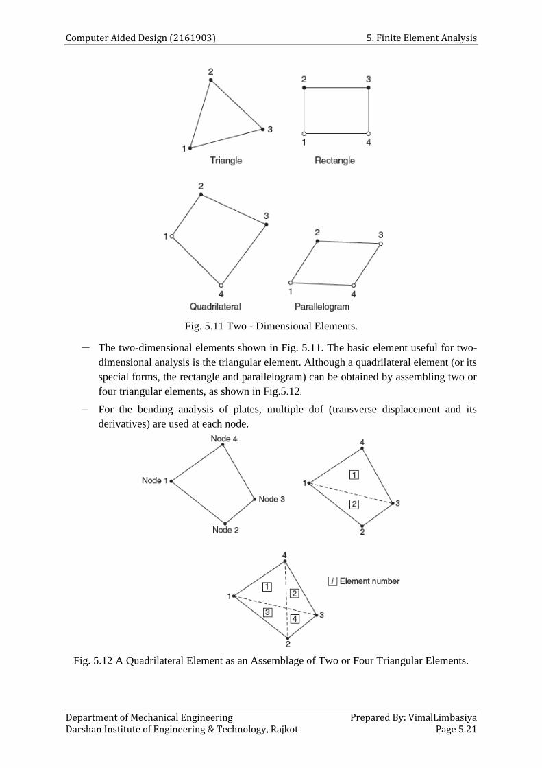
Computer Aided Design (2161903) 5. Finite Element Analysis
Department of Mechanical Engineering Prepared By: VimalLimbasiya Darshan Institute of Engineering & Technology, Rajkot Page 5.21
Fig. 5.11 Two - Dimensional Elements.
The two-dimensional elements shown in Fig. 5.11. The basic element useful for two-
dimensional analysis is the triangular element. Although a quadrilateral element (or its
special forms, the rectangle and parallelogram) can be obtained by assembling two or
four triangular elements, as shown in Fig.5.12.
For the bending analysis of plates, multiple dof (transverse displacement and its
derivatives) are used at each node.
Fig. 5.12 A Quadrilateral Element as an Assemblage of Two or Four Triangular Elements.

5. Finite Element Analysis Computer Aided Design (2161903)
Prepared By: VimalLimbasiya Department of Mechanical Engineering Page 5.22 Darshan Institute of Engineering & Technology, Rajkot
If the geometry, material properties, and other parameters of the body can be
described by three independent spatial coordinates, we can idealize the body by using
the three-dimensional elements shown in Fig.5.13.
Fig. 5.13Three-Dimensional Finite Elements.
The basic three-dimensional element, analogous to the triangular element in the case
of two-dimensional problems, is the tetrahedron element.
In some cases the hexahedron element, which can be obtained by assembling five
tetrahedrons as indicated in Fig. 5.14.

Computer Aided Design (2161903) 5. Finite Element Analysis
Department of Mechanical Engineering Prepared By: VimalLimbasiya Darshan Institute of Engineering & Technology, Rajkot Page 5.23
Fig. 5.14 A Hexahedron Element as an Assemblage of Five Tetrahedron Elements.
Some problems, which are actually three-dimensional, can be described by only one
or two independent coordinates. Such problems can be idealized by using an
axisymmetric or ring type of elements shown in Fig. 5.15.
Fig. 5.15 Axisymmetric Elements.
The problems that possess axial symmetry, such as pistons, storage tanks, valves,
rocket nozzles, and reentry vehicle heat shields, fall into this category.
For the discretization of problems involving curved geometries, finite elements with
curved sides are useful. Typical elements having curved boundaries are shown in Fig.
5.16.

5. Finite Element Analysis Computer Aided Design (2161903)
Prepared By: VimalLimbasiya Department of Mechanical Engineering Page 5.24 Darshan Institute of Engineering & Technology, Rajkot
Fig. 5.16 Finite Elements with Curved Boundaries.
5.10Discretization Process
Step - 1 :Type of Elements
If the problem involves the analysis of a truss structure under a given set of load
conditions (Fig. 5.17(a)), the type of elements to be used for idealization is obviously
the “bar or line elements” as shown in Fig. 5.17(b).
Fig. 5.17 A Truss Structure.

Computer Aided Design (2161903) 5. Finite Element Analysis
Department of Mechanical Engineering Prepared By: VimalLimbasiya Darshan Institute of Engineering & Technology, Rajkot Page 5.25
In the case of stress analysis of the short beam shown in Fig.5.18(a), the finite element
idealization can be done using three-dimensional solid elements as shown in Fig.
5.18(b).
Fig. 5.18 A Short Beam
In some cases one has to choose the type of elements judicially. As an example,
consider the problem of analysis of the thin walled shell shown in Fig. 5.19(a). In this
case, the shell can be idealized by several types of elements as shown in Fig. 5.19(b).
Fig. 5.19 A Thin-Walled Shell underPressure.

5. Finite Element Analysis Computer Aided Design (2161903)
Prepared By: VimalLimbasiya Department of Mechanical Engineering Page 5.26 Darshan Institute of Engineering & Technology, Rajkot
In some cases, we may have to use two or more types of elements for idealization. An
example of this would be the analysis of an aircraft wing.
Since the wing consists of top and bottom covers, Stiffening webs, andflanges, three
types of elements—namely, triangular plate elements (for covers),rectangular shear
panels (for webs), and frame elements (for flanges)—have been used in the idealization
shown in Fig. 5.20.
Fig. 5.20 Idealization of an AircraftWing Using Different Typesof Elements.
Step - 2 :Size of Elements
The size of elements influences the convergence of the solution directly, and hence it
has to be chosen with care.
If the size of the elements is small, the final solution is expected to be more accurate.
However, we have to remember that the use of smaller-sized elements will also mean
more computation time.
Sometimes, we may have to use elements of different sizes in the same body. For
example, in the case of stress analysis of the box beam shown in Fig. 5.21(a), the size
of all the elements can be approximately the same, as shown in Fig. 5.21(b).
However, in the case of stress analysis of a plate with a hole shown in Fig. 5.22 (a),
elements of different sizes have to be used, as shown in Fig. 5.22 (b). The size of
elements has to be very small near the hole (where stress concentration is expected)
compared to distant places.

Computer Aided Design (2161903) 5. Finite Element Analysis
Department of Mechanical Engineering Prepared By: VimalLimbasiya Darshan Institute of Engineering & Technology, Rajkot Page 5.27
Fig. 5.21A Box Beam.
Fig. 5.22 A Plate with a Hole.
The aspect ratio describes the shape of the element in the assemblage of elements.
For two-dimensional elements, the aspect ratio is taken as the ratio of the largest
dimension of the element to the smallest dimension. Elements with an aspect ratio of
nearly unity generally yield best results.
Step - 3 :Location of Nodes
Fig. 5.23 Location of Nodes at Discontinuities.

5. Finite Element Analysis Computer Aided Design (2161903)
Prepared By: VimalLimbasiya Department of Mechanical Engineering Page 5.28 Darshan Institute of Engineering & Technology, Rajkot
If the body has no abrupt changes in geometry, material properties, and external
conditions (e.g., load and temperature), the body can be divided into equal
subdivisions and hence the spacing of the nodes can be uniform.
On the other hand, if there are any discontinuities in the problem, nodes have to be
introduced at these discontinuities, as shown in Fig. 5.23.
Step - 4 :Number of Elements
The number of elements to be chosen for idealization is related to the accuracy
desired, size of elements, and the number of dof involved.
Although an increase in the number of elements generally means more accurate
results, for any given problem, there will be a certain number of elements beyond
which the accuracy cannot be significantly improved. This behavior is shown
graphically in Fig. 5.24.
Moreover, since the use of a large number of elements involves a large number of dof,
we may not be able to store the resulting matrices in the available computer memory.
Fig. 5.24 Effect of Varying the Number of Elements.
Step - 5 :Simplifications Afforded by the Physical Configuration of the Body
If the configuration of the body as well as the external conditions are symmetric, we
may consider only half of the body for finite element idealization. The symmetry
conditions, however, have to be incorporated in the solution procedure.
This is illustrated in Fig. 5.25,where only half of the plate with a hole, having
symmetry in both geometry and loading, is considered for analysis. Since there cannot
be a horizontal displacement along the line of symmetry AA, the condition that u = 0
has to be incorporated while finding the solution.

Computer Aided Design (2161903) 5. Finite Element Analysis
Department of Mechanical Engineering Prepared By: VimalLimbasiya Darshan Institute of Engineering & Technology, Rajkot Page 5.29
(a) Plate with hole (b) Only half of platecan be considered foranalysis
Fig. 5.25A Plate with a Hole withSymmetric Geometryand Loading.
Step - 6 :Finite Representation of Infinite Bodies
In most of the problems, like in the analysis of beams, plates, and shells, the
boundaries of the body or continuum are clearly defined. Hence, the entire body can
be considered for element idealization.
However, in some cases, as in the analysis of dams, foundations, and semi-infinite
bodies, the boundaries are not clearly defined. In the case of dams (Figure 5.26), since
the geometry is uniform and the loading does not change in the length direction, a unit
slice of the dam can be considered for idealization and analyzed as a plane strain
problem.
Fig. 5.26 A Dam with Uniform Geometry and Loading.

5. Finite Element Analysis Computer Aided Design (2161903)
Prepared By: VimalLimbasiya Department of Mechanical Engineering Page 5.30 Darshan Institute of Engineering & Technology, Rajkot
However, in the case of the foundation problem shown in Fig. 5.27(a), we cannot
idealize the complete semi-infinite soil by finite elements. Fortunately, it is not really
necessary to idealize the infinite body.
Since the effect of loading decreases gradually with increasing distance from the point
of loading, we can consider only that much of the continuum in which the loading is
expected to have a significant effect as shown in Fig. 5.27(b). Once the significant
extent of the infinite body is identified as shown in Fig. 5.27(b), the boundary
conditions for this finite body have to be incorporated in the solution.
Fig. 5.27 A Foundation underConcentrated Load.
5.11 Automatic Mesh Generation
Mesh generation is the process of dividing a physical domain into smaller subdomains
(called elements) to facilitate an approximate solution of the governing ordinary or
partial differential equation.
For this, one-dimensional domains (straight or curved lines) are subdivided into
smaller line segments, two-dimensional domains (planes or surfaces) are subdivided
into triangle or quadrilateral shapes, and three-dimensional domains (volumes) are
subdivided into tetrahedron and hexahedron shapes.
If the physical domain is simple and the number of elements used is small, mesh
generation can be done manually. However, most practical problems, such as those
encountered in aerospace, automobile, and construction industries have complex
geometries that require the use of thousands and sometimes millions of elements.
In such cases, the manual process of mesh generation is impossible and we have to
use automatic mesh generation schemes based on the use of a CAD or solid modeling
package.
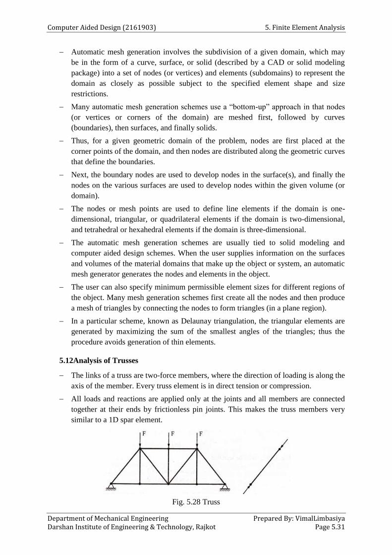
Computer Aided Design (2161903) 5. Finite Element Analysis
Department of Mechanical Engineering Prepared By: VimalLimbasiya Darshan Institute of Engineering & Technology, Rajkot Page 5.31
Automatic mesh generation involves the subdivision of a given domain, which may
be in the form of a curve, surface, or solid (described by a CAD or solid modeling
package) into a set of nodes (or vertices) and elements (subdomains) to represent the
domain as closely as possible subject to the specified element shape and size
restrictions.
Many automatic mesh generation schemes use a “bottom-up” approach in that nodes
(or vertices or corners of the domain) are meshed first, followed by curves
(boundaries), then surfaces, and finally solids.
Thus, for a given geometric domain of the problem, nodes are first placed at the
corner points of the domain, and then nodes are distributed along the geometric curves
that define the boundaries.
Next, the boundary nodes are used to develop nodes in the surface(s), and finally the
nodes on the various surfaces are used to develop nodes within the given volume (or
domain).
The nodes or mesh points are used to define line elements if the domain is one-
dimensional, triangular, or quadrilateral elements if the domain is two-dimensional,
and tetrahedral or hexahedral elements if the domain is three-dimensional.
The automatic mesh generation schemes are usually tied to solid modeling and
computer aided design schemes. When the user supplies information on the surfaces
and volumes of the material domains that make up the object or system, an automatic
mesh generator generates the nodes and elements in the object.
The user can also specify minimum permissible element sizes for different regions of
the object. Many mesh generation schemes first create all the nodes and then produce
a mesh of triangles by connecting the nodes to form triangles (in a plane region).
In a particular scheme, known as Delaunay triangulation, the triangular elements are
generated by maximizing the sum of the smallest angles of the triangles; thus the
procedure avoids generation of thin elements.
5.12Analysis of Trusses
The links of a truss are two-force members, where the direction of loading is along the
axis of the member. Every truss element is in direct tension or compression.
All loads and reactions are applied only at the joints and all members are connected
together at their ends by frictionless pin joints. This makes the truss members very
similar to a 1D spar element.
Fig. 5.28 Truss

5. Finite Element Analysis Computer Aided Design (2161903)
Prepared By: VimalLimbasiya Department of Mechanical Engineering Page 5.32 Darshan Institute of Engineering & Technology, Rajkot
The direction cosines l andm can be expressed as:
2 1cos
e
x xl
l
2 1cos sin
e
y ym
l
2 2
2 1 2 1( ) ( )el x x y y
q1‟ =qll + q2 m
q2‟ = q3 l + q4 m
Fig. 5.29 Direction Cosines
2 2
2 2
2 2
2 2
[ ] e e
e
l lm l lm
lm m lm mA EK
L l lm l lm
lm m lm m
e
e
El m l m q
l
Thermal Effect In Truss Member
(1) Thermal Load , P = e e e
l
mA E
l
m
(2) Stress for an element, ee
e
El m l m q E t
l
(3) Remaining steps will be same as earlier.
Example 5.6: A two member truss is as shown in Fig. 5.30. The cross-sectional area ofeach
member is 200 mm2 and the modulus of elasticity is 200 GPa. Determine the
deflections,reactions and stresses in each of the members.
Fig. 5.30

Computer Aided Design (2161903) 5. Finite Element Analysis
Department of Mechanical Engineering Prepared By: VimalLimbasiya Darshan Institute of Engineering & Technology, Rajkot Page 5.33
In globalterms, each node would have2 dof. These dof are marked as shown in Fig.5.31.
Theposition of the nodes, with respect to origin (considered at node l) are as tabulated below:
Node Xi Yi
1 0 0
2 4000 0
3 0 3000
Fig.5.31
For all elements, A=200 mm2
and E= 200 x 103 N/mm
2
The element connectivity table with the relevant terms are:
Element Ni Nj 2 2( ) ( )e j i j il x x y y e e
e
A E
l
j i
e
x xl
l
j i
e
y ym
l
l
2 m
2 lm
(1) 1 2 2 2(4000 0) (0 0)
4000
10000
4000 0
4000
1
0 00
4000
1 0 0
(2) 2 3 2 2(0 4000) (3000 0)
5000
8000
4000
5000
0.8
30000.6
5000 0.64 0.36 -0.48
As each node has two dof in global form, for every element, the element stiffness matrix
would be in a 4 x 4 form. For element 1 defined by nodes l-2,the dof are Q1, Q2, Q3 andQ4
and that for element 2 defined by nodes 2-3, would be Q3, Q4, Q5 andQ6. For a truss element
2 2
2 2
2 2
2 2
[ ]e e e
e
l lm l lm
lm m lm mA EK
L l lm l lm
lm m lm m
Element 1:The element stiffness matrix would be :

5. Finite Element Analysis Computer Aided Design (2161903)
Prepared By: VimalLimbasiya Department of Mechanical Engineering Page 5.34 Darshan Institute of Engineering & Technology, Rajkot
Element 2: The element stiffness matrix would be :
The global stiffness matrix would be :

Computer Aided Design (2161903) 5. Finite Element Analysis
Department of Mechanical Engineering Prepared By: VimalLimbasiya Darshan Institute of Engineering & Technology, Rajkot Page 5.35
In this case, node 1 and node 3 are completely fixed and hence,
Q1=Q2=Q5 = Q6 = 0
Hence, rows and columns 1,2,5 and 6 can be eliminated
Also the external nodal forces,
F1 = F2 = F3 = F5 = F6 = 0
F4 = -10 x 103 N
In global form, after using the elimination approach
103 (- 3.84 Q3 + 2.88 Q4) = - 10 x 10
3
- 3.84 Q3 + 2.88 Q4 = - l0
- 3.84 (0.254 Q4) + 2.88 Q4 = -10
Q4 = -5.25mm
Q3 = -1.334mm
The reactions can be found by using the equation:
R = KQ –F

5. Finite Element Analysis Computer Aided Design (2161903)
Prepared By: VimalLimbasiya Department of Mechanical Engineering Page 5.36 Darshan Institute of Engineering & Technology, Rajkot
R1 = -10 x 103 x (-1.334) = 13340 N
R2 = 0 N
R5 = -5.12 x 10³ x (-1.334) + 3.84 x 10
3x (-5.25) = -13340 N
R6 = 3.84 x 10³ x (-1.334) – 2.88 x 10
3x (-5.25) = 9997.44 N
To determine stresses: e
e
El m l m q
l
Element 1:
Element 2:
Example 5.7:Consider the four-bar truss shown in Fig. 5.32(a). It is given that E = 29.5 x 10⁶
psi andAe = lin.2 for all elements. Complete the following:
(a) Determine the element stiffness matrix for each element.
(b) Assemble the structural stiffness matrix K for the entire truss
(c) Using the elimination approach, solve for the nodal displacement.
(d) Recover the stresses in each element.
(e) Calculate the reaction forces.

Computer Aided Design (2161903) 5. Finite Element Analysis
Department of Mechanical Engineering Prepared By: VimalLimbasiya Darshan Institute of Engineering & Technology, Rajkot Page 5.37
(a)
(b)
Fig. 5.32
(a) It is recommended that a tabular form be used for representing nodal coordinate data
and element information. The nodal coordinate data are as follows:
Node x y
1 0 0
2 40 0
3 40 30
4 0 30
The element connectivity table is
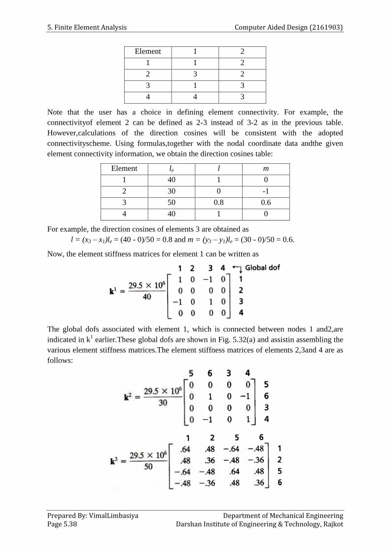
5. Finite Element Analysis Computer Aided Design (2161903)
Prepared By: VimalLimbasiya Department of Mechanical Engineering Page 5.38 Darshan Institute of Engineering & Technology, Rajkot
Element 1 2
1 1 2
2 3 2
3 1 3
4 4 3
Note that the user has a choice in defining element connectivity. For example, the
connectivityof element 2 can be defined as 2-3 instead of 3-2 as in the previous table.
However,calculations of the direction cosines will be consistent with the adopted
connectivityscheme. Using formulas,together with the nodal coordinate data andthe given
element connectivity information, we obtain the direction cosines table:
Element le l m
1 40 1 0
2 30 0 -1
3 50 0.8 0.6
4 40 1 0
For example, the direction cosines of elements 3 are obtained as
l = (x3 – x1)le = (40 - 0)/50 = 0.8 and m = (y3 – y1)le = (30 - 0)/50 = 0.6.
Now, the element stiffness matrices for element 1 can be written as
The global dofs associated with element 1, which is connected between nodes 1 and2,are
indicated in k1 earlier.These global dofs are shown in Fig. 5.32(a) and assistin assembling the
various element stiffness matrices.The element stiffness matrices of elements 2,3and 4 are as
follows:

Computer Aided Design (2161903) 5. Finite Element Analysis
Department of Mechanical Engineering Prepared By: VimalLimbasiya Darshan Institute of Engineering & Technology, Rajkot Page 5.39
(b) The structural stiffness matrix K is now assembled from the element stiffness
matrices.By adding the element stiffness contributions, noting the element
connectivity, we get
(c) The structural stiffness matrix K given above needs to be modified to account for the
boundary conditions. The elimination approach will be used here. The rows and
columns corresponding to dofs 1, 2, 4, 7, and 8, which correspond to fixed supports,
are deleted from the K matrix. The reduced finite element equations are given as
Solution of these equations yields the displacements
The nodal displacement vector for the entire structure can therefore be written as
Q =[0, 0,27.12x 10-3
, 0,5.65 x 10-3
, -22.25 x 10⁻³
,0, 0]T in.
(d) The stress in each element can now be determined as shown below.
The connectivity of element 1 is 1 - 2. Consequently, the
nodaldisplacementvectorforelementlisgivenby q = [0,0, 27.72 x 10⁻³
,0]T
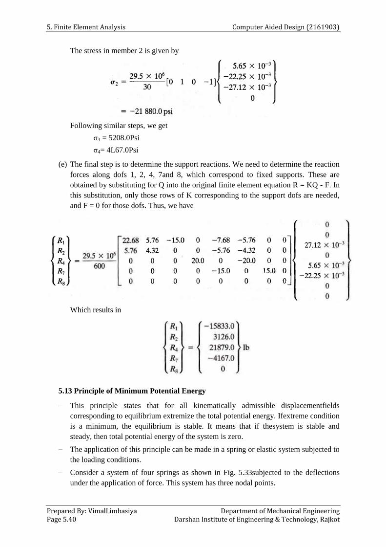
5. Finite Element Analysis Computer Aided Design (2161903)
Prepared By: VimalLimbasiya Department of Mechanical Engineering Page 5.40 Darshan Institute of Engineering & Technology, Rajkot
The stress in member 2 is given by
Following similar steps, we get
ζ3 = 5208.0Psi
ζ4= 4L67.0Psi
(e) The final step is to determine the support reactions. We need to determine the reaction
forces along dofs 1, 2, 4, 7and 8, which correspond to fixed supports. These are
obtained by substituting for Q into the original finite element equation R = KQ - F. In
this substitution, only those rows of K corresponding to the support dofs are needed,
and F = 0 for those dofs. Thus, we have
Which results in
5.13 Principle of Minimum Potential Energy
This principle states that for all kinematically admissible displacementfields
corresponding to equilibrium extremize the total potential energy. Ifextreme condition
is a minimum, the equilibrium is stable. It means that if thesystem is stable and
steady, then total potential energy of the system is zero.
The application of this principle can be made in a spring or elastic system subjected to
the loading conditions.
Consider a system of four springs as shown in Fig. 5.33subjected to the deflections
under the application of force. This system has three nodal points.
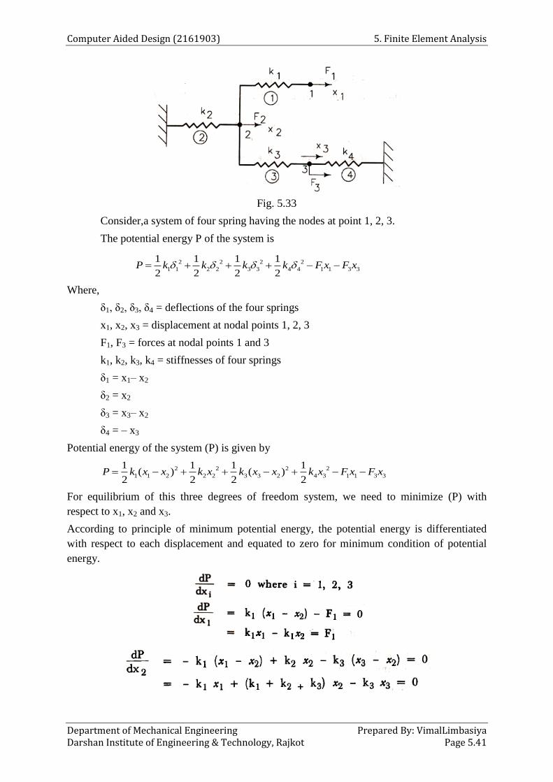
Computer Aided Design (2161903) 5. Finite Element Analysis
Department of Mechanical Engineering Prepared By: VimalLimbasiya Darshan Institute of Engineering & Technology, Rajkot Page 5.41
Fig. 5.33
Consider,a system of four spring having the nodes at point 1, 2, 3.
The potential energy P of the system is
2 2 2 2
1 1 2 2 3 3 4 4 1 1 3 3
1 1 1 1
2 2 2 2P k k k k F x F x
Where,
δ1, δ2, δ3, δ4 = deflections of the four springs
x1, x2, x3 = displacement at nodal points 1, 2, 3
F1, F3 = forces at nodal points 1 and 3
k1, k2, k3, k4 = stiffnesses of four springs
δ1 = x1– x2
δ2 = x2
δ3 = x3– x2
δ4 = – x3
Potential energy of the system (P) is given by
2 2 2 2
1 1 2 2 2 3 3 2 4 3 1 1 3 3
1 1 1 1( ) ( )
2 2 2 2P k x x k x k x x k x F x F x
For equilibrium of this three degrees of freedom system, we need to minimize (P) with
respect to x1, x2 and x3.
According to principle of minimum potential energy, the potential energy is differentiated
with respect to each displacement and equated to zero for minimum condition of potential
energy.

5. Finite Element Analysis Computer Aided Design (2161903)
Prepared By: VimalLimbasiya Department of Mechanical Engineering Page 5.42 Darshan Institute of Engineering & Technology, Rajkot
…….(4)
The x1, x2, x3deflectionscanbeobtainedbyusing numerical methods.
On the other hand, we proceed to write the equilibrium equations of the system by
considering the equilibrium of each separate node as shown in Fig. 5.34.
k1δ1 = F1
k2δ2 – k1δ1 – k3δ3 = 0
k3δ3 – k4δ4 = F3
which is precisely the set of equations represented in Eq. (4).
Fig. 5.34.
We see clearly that the set of equations (4) is obtained in a routine manner using thepotential
energy approach,without any reference to the free-body diagrams. This makes thepotential
energy approach attractive for large and complex problems.
Example 5.8: Calculate the deflections of the points at node 1, 2 and 3 for the spring system
shown in Fig. 5.33. The stiffnesses are k1 = 80 N/mm, k2= 50 N/mm, k3=60 N/mm, k4 = 40
N/mm, the loads are F1= 40 N, F3 = 60 N.
Find the deflections x1, x2 and x3.
The model of the above system is used and stiffness, deflection and load matrix can be
written as

Computer Aided Design (2161903) 5. Finite Element Analysis
Department of Mechanical Engineering Prepared By: VimalLimbasiya Darshan Institute of Engineering & Technology, Rajkot Page 5.43
Solving the above matrices, the value of x1= 0.4 mm, x2= 0.1 mm, x3= 0.66 mm.
Example 5.9: Fig. 5.35 shows a cluster of four springs. One end of the assembly is fixed and
a force of 1000 N is applied at the end. Using the finite element method, determine:
(a) The deflection of each spring.
(b) The reaction forces at support.
Fig. 5.35
The system of springs can be represented by a finite element model as shown in Fig. 5.36
Fig. 5.36
The element connectivity table is as shown:
The element stiffness matrices are as under:

5. Finite Element Analysis Computer Aided Design (2161903)
Prepared By: VimalLimbasiya Department of Mechanical Engineering Page 5.44 Darshan Institute of Engineering & Technology, Rajkot
The overall stiffness matrix would be:
In global terms,
The boundary conditions for this problem are:
Q1 = 0
F1 = F2 = 0
F3 = 1000 N
By elimination approach:
22 Q2 – 10 Q3 = 0
Q2 = 0.4545 Q3

Computer Aided Design (2161903) 5. Finite Element Analysis
Department of Mechanical Engineering Prepared By: VimalLimbasiya Darshan Institute of Engineering & Technology, Rajkot Page 5.45
– 10 Q2 + 30 Q3 = 1000
– 10 (0.4545 Q3) + 30 Q3 = 1000
Q3 = 39.286 mm
Q2 = 0.4545 x 39.286 = 17.857 mm
To determine the reaction forces,
R = KQ – F
5.14 Natural OR Intrinsic Coordinate System:
Fig.5.37
Consider a element (e), having node numbers 1 & 2 shown in Fig. 5.37 (a). The first node
1 would be at a distance x1 and second node would be at a distance x2 from the reference.
A convenient coordinate system called as the natural coordinate system is defined, as it
helps in formulating individual element matrix which can than be used to combine and
form a global stiffness matrix.
In natural coordinate system, the centre of the element is considered as 0 and the node 1
and node 2 are placed at a distance - 1 and + 1 respectively Fig. 5.37(b). The variable of
measurement of the distance in this case is represented as ξ. Thus node 1 is at coordinate
position ξ = - 1 and node 2 is at ξ = + 1. Total length of the element would thus be 2 units
and this length of the element is covered in the range ξ = - 1 to +1.
To establish relationship between two coordinate system consider any point P situated at a
distance x, in the Global coordinate system Fig.5.37 (a) and correspondingly at a distance
ξ from the origin as shown in Fig.5.37 (b).
Now
Length of element in Natural system Dist. of Point P from Node in Natural system
Length of element in Global system Dist. of Point P from Node in Global system
1
1

5. Finite Element Analysis Computer Aided Design (2161903)
Prepared By: VimalLimbasiya Department of Mechanical Engineering Page 5.46 Darshan Institute of Engineering & Technology, Rajkot
x x x x2 1 1
2 1
x x_______(a)
x x
1
2 1
21
Confirm the validity of equation (a)
1 1
1
2 1
2 x xAt x = x ξ = 1 = 0 1= 1
x x
x xAt x x
x x
2 12
2 1
21 2 1 1
This confirm the relation of the two coordinate system.
5.15 Shape function in Natural Coordinate System:
The natural coordinate can be used to define shape functions. This makes it convenient to
isolate the element from the continuum and develop the necessary element stiffness
matrix. The shape function as defined earlier is used to interpolate the deflections or
degree of freedom within the element. The accuracy of calculations would increase with
increase in number of elements. Consider linear distribution as represented by Fig.5.38.
Fig.5.38
The shape function N1 and N2 in natural coordinate term can be developed by considering
Fig.5.39 (a) and Fig.5.39 (b).
Fig.5.39

Computer Aided Design (2161903) 5. Finite Element Analysis
Department of Mechanical Engineering Prepared By: VimalLimbasiya Darshan Institute of Engineering & Technology, Rajkot Page 5.47
Fig. 5.39 (a) General line equation is
m slopey mx C
For N ,1
1
2
1 1
N C
( ) C C
N
N
1
1
1
1
2
1 11 1
2 2
1 1
2 2
1
2
Fig. 5.39(b) line equation is
m slopey mx C
For N ,2
1
2
0 1
N C
( ) C
C
N
N
2
2
2
1
2
10 1
2
1
2
1 1
2 2
1
2
Once the shape functions are defined, the linear displacement field within the element can
be written in terms of nodal displacements q1 and q2 as….
1 1 2 2u N q N q ........ (b)
Fig.5.40

5. Finite Element Analysis Computer Aided Design (2161903)
Prepared By: VimalLimbasiya Department of Mechanical Engineering Page 5.48 Darshan Institute of Engineering & Technology, Rajkot
which in Matrix form will be
1 2
1T
1 2
2
u N q
where N N , N
qq q , q
q
The term q is referred to as element displacement vector, and the verification of equation
(b) can be done by considering the equation of shape functions.
At Node 1: 1
1
2
1 1 ( 1)N 1
2 2
1 1 ( 1)N 0
2 2
So displacement at Node 1 will be
1 1 2 2
1 2
1
u N q N q
1(q ) 0 (q )
q
At Node 2: 1
1
2
1 1 1N 0
2 2
1 1 1N 1
2 2
So displacement at Node 2 will be
2 2 1 1
2 1
2
u N q N q
1(q ) 0 (q )
q
Thus it is seen that as per equation, the displacement at Node 1 and 2 are q1 and q2 which
are the expected results.
We know equation
1
2 1
2 x x1
x x
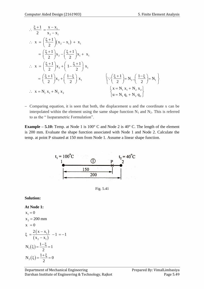
Computer Aided Design (2161903) 5. Finite Element Analysis
Department of Mechanical Engineering Prepared By: VimalLimbasiya Darshan Institute of Engineering & Technology, Rajkot Page 5.49
Comparing equation, it is seen that both, the displacement u and the coordinate x can be
interpolated within the element using the same shape function N1 and N2. This is referred
to as the “ Isoparametric Formulation”.
Example – 5.10: Temp. at Node 1 is 100° C and Node 2 is 40° C. The length of the element
is 200 mm. Evaluate the shape function associated with Node 1 and Node 2. Calculate the
temp. at point P situated at 150 mm from Node 1. Assume a linear shape function.
Fig. 5.41
Solution:
At Node 1:
1
2
1
2 1
1
2
x 0
x 200 mm
x 0
2 x x1 1
x x
1N 1
2
1N 0
2
1
2 1
2 1 1
2 1 1
2 1
2 1 2 1
1 1 2 2
1 1 2 2
1 1 2 2
x x1
2 x x
1x x x x
2
1 1x x x
2 2
1 1x x 1 x
2 2
1 1 1 1x x N , N
2 2 2 2
x N x N xx N x N x
u N q N q

5. Finite Element Analysis Computer Aided Design (2161903)
Prepared By: VimalLimbasiya Department of Mechanical Engineering Page 5.50 Darshan Institute of Engineering & Technology, Rajkot
At Node 2:
1
2
1
2 1
1
2
x 0
x 200 mm
x 200 mm
2 x x 2 200 01 1 1
x x 200 0
1N 0
2
1N 1
2
At Point P:
1 1
2 2
x 0 t 100 C
x 200 mm t 40 C
x 150 mm
1
2 1
1
2
2 x x 2 150 01 1 0.5
x x 200 0
1 1 0.5N 0.25
2 2
1 1 0.5N 0.75
2 2
1 1 2 2t N t N t
0.25 100 0.75 40
t 55 C
Example – 5.11 : A 1D spar element having a linear shape function as shown in fig. If the
temp.at Node 1 is 50° C and Node 2 is -20°C. Find the temp. at point P.
Fig. 5.42
Solution:
At Point P:
1 1
2 2
x 25 t 50 C
x 50 t 20 C
x 30

Computer Aided Design (2161903) 5. Finite Element Analysis
Department of Mechanical Engineering Prepared By: VimalLimbasiya Darshan Institute of Engineering & Technology, Rajkot Page 5.51
Let
1
2 1
2 x x 2 30 251 1 0.6
x x 50 25
Now
1
2
1 0.61N 0.8
2 2
1 0.61N 0.2
2 2
1 1 2 2t N t N t
0.8 50 0.2 20
t 30 C
Example – 5.12: Consider an element having a linear shape function shown in fig. Evaluate
the natural coordinate and shape functions for point P. If the displacement at Node 1 and
Node 2 are 2 mm and -1 mm respectively, determine the value of displacement at point P.
Also determine in global terms the point where the displacement would be zero. Also
determine the shape function at zero displacement point.
Fig. 5.43
Solution:
At point P:
1 1
2 2
x 180 mm q 2 mm
x 360 mm q 1 mm
x 220 mm
Let
1
2 1
1
2
2 x x 2 220 1801 1 0.556
x x 360 180
1 0.5561N 0.778
2 2
1 0.5561N 0.222
2 2
Let

5. Finite Element Analysis Computer Aided Design (2161903)
Prepared By: VimalLimbasiya Department of Mechanical Engineering Page 5.52 Darshan Institute of Engineering & Technology, Rajkot
1 1 2 2u N q N q
0.778 2 0.222 1
u 1.334 mm
To determine the position of point where displacement is zero (q1 = 2 mm , q2 = -1 mm).
Let
1 1 2 2
1 2
1 2
u N q N q
0 N 2 N 1
2 N N
1 12
2 2
2 2 1
10.333
3
Let
1
2 1
2 x x1
x x
2 x 1800.333 1
360 180
x 300 mm
1
2 1
1 1 0.333N 0.333
2 2
N 2 N 2 (0.333) 0.667
x can be find out
1 1 2 2x N x N x
0.333 180 0.667 360
x 300 mm
Example – 5.13: Determine the temperature at x = 40 mm if the temperature at nodes Øi =
120° C and Øj = 80° C and xi = 10 mm, xj = 60 mm.
Fig. 5.44

Computer Aided Design (2161903) 5. Finite Element Analysis
Department of Mechanical Engineering Prepared By: VimalLimbasiya Darshan Institute of Engineering & Technology, Rajkot Page 5.53
Solution:
i
j
i
j
x 10
x 60
1x 40
2
120 C
80 C
Let
1
2 1
2 x x1
x x
2 40 101
60 10
0.2
1
2
1 1 0.2N 0.4
2 2
1 1 0.2N 0.6
2 2
Let
1 i 2 jN N
0.4 120 0.6 80
96 C
References:
Finite Element Method – S.S. Rao
Introduction to Finite Elements in Engineering - Tirupathi R. Chandrupatla
CAD/CAM & Automation – FarazdakHaideri
CAD/CAM – Khandare