Embed Size (px)
Citation preview

Introduction to causal inference and causalmediation analysis
Donna SpiegelmanDepartments of Epidemiology, Biostatistics, Nutrition and Global
HealthHarvard T.H. Chan School of Public Health
Boston, MAUSA
with Daniel Nevo and Xiaomei Liao

Outline
Introduction to causal inference
Introduction to causal mediation analysis.
Unified framework for the difference method in GLMs
g-linkability results
Data duplication algorithm
Simulations, an example and summary.
Donna Spiegelman Introduction to causal inference and causal mediation analysisJanuary 2, 2018 2 / 30

Counterfactual outcomes
An intervention, X , and an outcome which it may cause, Y .Y canbe a health outcome or a process outcome.
Counterfactuals: Yi(x) defined for each value of x .
We observe one value only for each participant i . If X is binary, weobserve either Yi(0) or Yi(1). This is the “fundamental problem ofcausal inference”
Neyman (1923); Rubin (1974,1980); Holland (1986); Robins (1986)
Donna Spiegelman Introduction to causal inference and causal mediation analysisJanuary 2, 2018 3 / 30
Average causal effect
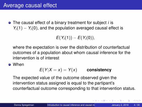
The causal effect of a binary treatment for subject i isYi(1)− Yi(0), and the population averaged causal effect is
E(Yi(1))− E(Yi(0)),
where the expectation is over the distribution of counterfactualoutcomes of a population about whom causal inference for theintervention is of interestWhen
E(Y |X = x) = Y (x) consistency
The expected value of the outcome observed given theintervention status assigned is equal to the partipant’scounterfactual outcome corresponding to that intervention status.
Donna Spiegelman Introduction to causal inference and causal mediation analysisJanuary 2, 2018 4 / 30
Average causal effect
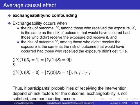
exchangeability/no confounding
Exchangeability occurs whenthe risk of outcome, Y , among those who received the exposure, X ,is the same as the risk of outcome that would have occured hadthose who didn’t receive the exposure did receive it, andthe risk of outcome Y , among those who didn’t receive theexposure is the same as the risk of outcome that would haveoccurred had those who received the exposure didn’t get it, i.e.
([Yi(1)|Xi = 1] = [Yj(1)|Xj = 0])&
([Yi(0)|Xi = 0] = [Yj(0)|Xj = 1]),∀i , j , i 6= j
Thus, if participants’ probabilities of receiving the interventiondepend on risk factors for the outcome, exchangeability is notsatisfied, and confounding occursThis is why we love randomization!And why causal inference methods are needed for observationalstudies.
Donna Spiegelman Introduction to causal inference and causal mediation analysisJanuary 2, 2018 5 / 30
Conditional exchangeability
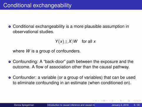
Conditional exchangeability is a more plausible assumption inobservational studies.
Y (x) |= X |W for all x
where W is a group of confounders.
Confounding: A “back-door” path between the exposure and theoutcome. A flow of association other than the causal pathway.
Confounder: a variable (or a group of variables) that can be usedto eliminate confounding in an estimate (when conditioned on).
Donna Spiegelman Introduction to causal inference and causal mediation analysisJanuary 2, 2018 6 / 30

Mediation Analysis
So a causal effect of X on Y was established, but we want more!
X M Y
The directed acyclic graph (DAG) above encodes assumptions.Nodes are variables, directed arrows depict causal pathways
Here M is caused by X , and Y is caused by both M and X .
DAGs can be useful for causal inference: clarify the assumptionstaken and facilitate the discussion.
Donna Spiegelman Introduction to causal inference and causal mediation analysisJanuary 2, 2018 7 / 30

Examples of mediation in practice
Does cognitive behavioral therapy (X ) targeting worry reducedelusions (Y )? Via worry reduction (M) ?
(Freeman et al., The Lancet Psychiatry, 2015)
Does tumor subtype and stage at diagnosis (M) mediate the effectof race (X) on post-diagnosis survival (Y)?
(Warner et al., J. Clin. Oncol., 2015)
Does percentage Mammographic Density (M) mediates risk factoreffects (e.g., BMI at age 18, X) on post-menopausal breast cancer(Y)?
(Rice et al., Breast Cancer Res., 2016)
Donna Spiegelman Introduction to causal inference and causal mediation analysisJanuary 2, 2018 8 / 30

Causal mediation analysis
X M Y
We need more counterfactuals: Mi(x) and Yi(x ,m) for all relevantx ,m values.
Composite counterfactuals: Yi(x) = Yi(x ,Mi(x))
For every x , the value of Mi is set according to the value X = x ,Mi(x), and then Yi(x ,Mi(x)) is obtained.
For example: If Mi(0) = 1, Yi(0) = Yi(0,1).
The total effect of X on Y
TE(x , x ′) = E [Y (x ′)]− E [Y (x)]= E [Y (x ′,M(x ′))]− E [Y (x ,M(x))]
Donna Spiegelman Introduction to causal inference and causal mediation analysisJanuary 2, 2018 9 / 30

Natural direct and indirect effects
X M Y
The natural direct effect NDE = E [Y (1,M(0))]− E [Y (0,M(0))]
The natural indirect effect
NIE = E [Y (1,M(1))]− E [Y (1,M(0))]
a Robins and Greenland (1992); Pearl (2001)
Donna Spiegelman Introduction to causal inference and causal mediation analysisJanuary 2, 2018 10 / 30

The mediation proportion
TE = E(Y (1,M(1)))− E(Y (0,M(0)))We have the following decomposition
TE = NDE + NIE
In practice, researchers prefer the mediation proportion
MP =NIETE
=NIE
NIE + NDE
Proportion if MP ∈ [0,1].
Donna Spiegelman Introduction to causal inference and causal mediation analysisJanuary 2, 2018 11 / 30
Mediation analysis with confounders
W1 X
W2
M
W3
YY
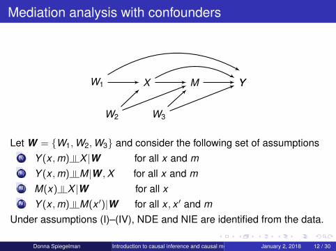
Let W = {W1,W2,W3} and consider the following set of assumptions(I) Y (x ,m) |= X |W for all x and m(II) Y (x ,m) |= M|W ,X for all x and m(III) M(x) |= X |W for all x(IV) Y (x ,m) |= M(x ′)|W for all x , x ′ and m
Under assumptions (I)–(IV), NDE and NIE are identified from the data.
Donna Spiegelman Introduction to causal inference and causal mediation analysisJanuary 2, 2018 12 / 30
Linear models for mediation
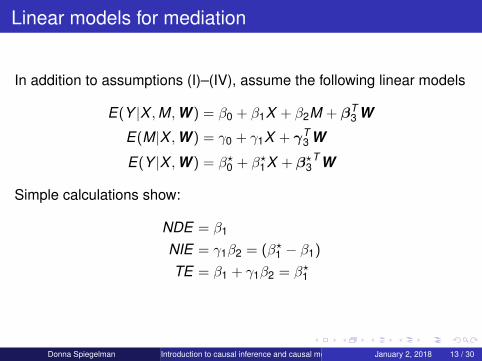
In addition to assumptions (I)–(IV), assume the following linear models
E(Y |X ,M,W ) = β0 + β1X + β2M + βT3 W
E(M|X ,W ) = γ0 + γ1X + γT3 W
E(Y |X ,W ) = β?0 + β?1X + β?3T W
Simple calculations show:
NDE = β1
NIE = γ1β2 = (β?1 − β1)
TE = β1 + γ1β2 = β?1
Donna Spiegelman Introduction to causal inference and causal mediation analysisJanuary 2, 2018 13 / 30

The product method and the difference method
E(Y |X ,M,W ) = β0 + β1X + β2M + βT3 W
E(M|X ,W ) = γ0 + γ1X + γT3 W
E(Y |X ,W ) = β?0 + β?1X + β?3T W
NIE = γ1β2 = β?1 − β1
MP =γ1β2
γ1β2 + β1=β?1 − β1
β?1
The NIE estimates β̂2γ̂1 and β̂?1 − β̂1 are the same, algebraically.
If Y is binary and we replace the outcome linear regressions bylogistic regressions this is no longer the case.
Asymptotic normality and variance: delta method and/orbootstrap.
Donna Spiegelman Introduction to causal inference and causal mediation analysisJanuary 2, 2018 14 / 30

Mediation analysis with GLMs
The difference method.
E(Y |X ,M,W ) = g−1(β0 + β1X + β2M + βT3 W )
E(Y |X ,W ) = g−1(β?0 + β?1X + β?3T W )
g(·) is a known link function. Examples: g(u) = u, g(u) = log(u)and g(u) = logit(u) = log(u/(1− u)).TE, NIE and NDE can be defined on the coefficient scale (onthe link function scale):
NIE = β?1 − β1 and MP = (β?1 − β1)/β?1
For example, for logistic regression, we have the samedecomposition, different interpretation:
logORTE = logORNDE + logORNIE
VanderWeele and Vansteelandt (2010)
Donna Spiegelman Introduction to causal inference and causal mediation analysisJanuary 2, 2018 15 / 30

Generalized linear models (GLMs)
E(Y |X ,M,W ) = g−1(β0 + β1X + β2M + βT3 W )
E(Y |X ,W ) = g−1(β?0 + β?1X + β?3T W )
Estimate β = (β0, β1, β2,β3) and β? = (β?0, β?1,β
?3) by solving
U(β) =
{ ∑ni=1 DT
i v−1i [Yi − E(Yi |Xi ,Mi ,W i)]∑n
i=1 D?Ti v?i −1[Yi − E(Yi |X ?
i ,W?i )]
}= 0
where D i = ∂E(Yi |Xi ,Mi ,W i)/∂β and vi is the variance of Yi .
Question: Does the same link function g hold for both models?
Donna Spiegelman Introduction to causal inference and causal mediation analysisJanuary 2, 2018 16 / 30

g-linkability
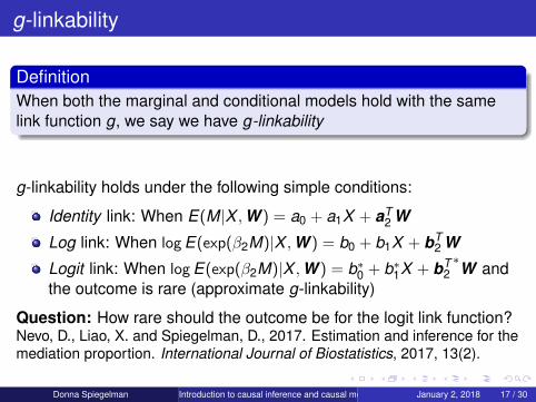
DefinitionWhen both the marginal and conditional models hold with the samelink function g, we say we have g-linkability
g-linkability holds under the following simple conditions:
Identity link: When E(M|X ,W ) = a0 + a1X + aT2 W
Log link: When logE(exp(β2M)|X ,W ) = b0 + b1X + bT2 W
Logit link: When logE(exp(β2M)|X ,W ) = b∗0 + b∗1X + bT2∗W and
the outcome is rare (approximate g-linkability)
Question: How rare should the outcome be for the logit link function?Nevo, D., Liao, X. and Spiegelman, D., 2017. Estimation and inference for themediation proportion. International Journal of Biostatistics, 2017, 13(2).
Donna Spiegelman Introduction to causal inference and causal mediation analysisJanuary 2, 2018 17 / 30
g-linkability
DefinitionWhen both the marginal and conditional models hold with the samelink function g, we say we have g-linkability
g-linkability holds under the following simple conditions:
Identity link: When E(M|X ,W ) = a0 + a1X + aT2 W
Log link: When logE(exp(β2M)|X ,W ) = b0 + b1X + bT2 W
Logit link: When logE(exp(β2M)|X ,W ) = b∗0 + b∗1X + bT2∗W and
the outcome is rare (approximate g-linkability)
Question: How rare should the outcome be for the logit link function?Nevo, D., Liao, X. and Spiegelman, D., 2017. Estimation and inference for themediation proportion. International Journal of Biostatistics, 2017, 13(2).
Donna Spiegelman Introduction to causal inference and causal mediation analysisJanuary 2, 2018 17 / 30

Rare outcome assumption
Pr(Y = 1) = 0.005 Pr(Y = 1) = 0.01 Pr(Y = 1) = 0.1 Pr(Y = 1) = 0.25
0.2
0.4
0.6
0.8
0.2
0.4
0.6
0.8
0.2
0.4
0.6
0.8
E(Ncases )
=100
E(Ncases )
=500
E(Ncases )
=1000
0.2 0.4 0.6 0.8 0.2 0.4 0.6 0.8 0.2 0.4 0.6 0.8 0.2 0.4 0.6 0.8p
ρ
relative bias<=1%1%−5%5%−10%10%−25%25%−50%>=50%
Binary outcome; TE = log(β?1 ) = log(1.5). (X ,M) jointly normal,ρ = cor(X ,M). Relative bias: |mean(M̂P)−MP|/MP.
Donna Spiegelman Introduction to causal inference and causal mediation analysisJanuary 2, 2018 18 / 30

Inference for mediation parameters: difference method
Testing for mediation: H0 : NIE = β?1 − β1 = 0 orH0 : MP = (β?1 − β1)/β
?1 = 0. CIs are also of interest.
Asymptotic normality and variance by the delta method
Var(N̂IE) = Var(β̂?1) + Var(β̂1)− 2Cov(β̂?1, β̂1)
Var(M̂P) =β2
1Var(β̂?1)(β?1)
4 +Var(β̂1)
(β?1)2 − 2
β1
(β?1)3 Cov(β̂1, β̂
?1)
If we had estimates for Var(M̂P) and Var(N̂IE), we could haveconstructed confidence intervals and (one-sided) Z-tests formediation.How to estimate Cov(β̂?1, β̂1)? Must bootstrap?
Donna Spiegelman Introduction to causal inference and causal mediation analysisJanuary 2, 2018 19 / 30

Inference: Data duplication algorithm
How to estimate Cov(β̂?1, β̂1)?The idea: Fit a single model that includes β?1 and β1. For j = 1,2:
E(Yij |Xi ,Mi ,W i) =
g−1
[I{j = 1}(β0 + β1Xi + β2Mi + βT
3 W i) + I{j = 2}(β?0 + β?1 Xi + β?T3 W i)
]
Use generalized estimating equations (GEE) to estimate (βT , β∗T )from the duplicated data.Create a duplicated dataset: each observation is represented bytwo pseudo-observations and each of the covariates appearstwice. The mediator is not duplicated. Set values to zerosaccording to the above model.The SAS macro %mediate implements the data duplicationalgorithm.Donna Spiegelman Introduction to causal inference and causal mediation analysisJanuary 2, 2018 20 / 30

Data duplication
i j Intercept Intercept? X X? M W W ? Y1 1 1 0 x1 0 m1 w1 0 y11 2 0 1 0 x1 0 0 w1 y12 1 1 0 x2 0 m2 w2 0 y22 2 0 1 0 x2 0 0 w2 y2...
......
......
......
......
...
For each i , j = 1 observation comes from the conditional modeland j = 2 from the marginal model.Fit for the duplicated data the model
E(Yij |Xi ,X ?i ,Mi ,W i ,W ?
i ) =
g−1(β0I{j = 1}+ β1Xi + β2Mi + βT
3 W i + β?0 I{j = 2}+ β?1 X ?i + β?T
3 W ?i
)We get a consistent estimator for Cov(β̂, β̂?), just by looking in theright place in the sandwich estimator matrix.
Donna Spiegelman Introduction to causal inference and causal mediation analysisJanuary 2, 2018 21 / 30

GEE for the duplicated data
Testing: Reject two-sided test H0 : MP = 0 if∣∣∣∣M̂P/√
V̂ar(M̂P)
∣∣∣∣ > z1−α/2
alternative test: ∣∣∣∣N̂IE/√
V̂ar(N̂IE)
∣∣∣∣ > z1−α/2
Confidence interval:
M̂P ±√
V̂ar(M̂P) · z1−α/2
Donna Spiegelman Introduction to causal inference and causal mediation analysisJanuary 2, 2018 22 / 30

Software for causal mediation analysis
SAS Macro %mediate and R package (on CRAN) GEEmediateimplement the data duplication algorithm, and reports point estimates,CIs and p-values for MP and NIE. Very fast implementation becausethey take advantage of existing software (PROC GENMOD or geepackage).
Nevo, D., Liao, X. and Spiegelman, D., 2017. Estimation and inferencefor the mediation proportion. International Journal of Biostatistics,2017, 13(2)
Macro available at:https://www.hsph.harvard.edu/donna-spiegelman/software/mediate/
Donna Spiegelman Introduction to causal inference and causal mediation analysisJanuary 2, 2018 23 / 30
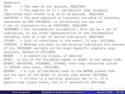
%mediate(DATA = The name of the dataset. REQUIREDID = The name(s) of >= 1 variable(s) that uniquelyidentifies each record (e.g id or id period). REQUIREDEXPOSURE = The main exposure or treatment variable of interest,expressed as ONE VARIABLE, or alternately you may usea set of indicators for an EXPOSURE. REQUIREDINTERMED = The intermediate variable(s). This can be a set ofindicators, or any other representation of the intermediatevariable, such as a set of spline indicators. REQUIREDCOVARS = List of covariates in the model, if any. OPTIONALINTMISS = Whether you want to use missing indicators for unknown valuesof the INTERMED variable vs the model-specific complete caseanalysis. Default=F OPTIONALWHERE = A subsetting clause, if desiredNOTE: if any of the variables named in WHERE is not among TIME,EVENT, EXPOSURE, INTERMED, COVARS, then they should be listedin EXTRAV (see next). OPTIONALEXTRAV = A list of variables used in the WHERE clause thatare not part of the model or strata (see above) OPTIONALSURV = If this is a survival analysis set to T, if ageneralized linear model, set to F (default=T) OPTIONAL
Donna Spiegelman Introduction to causal inference and causal mediation analysisJanuary 2, 2018 23 / 30
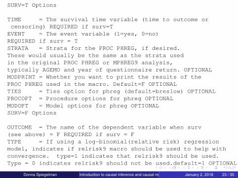
SURV=T Options
TIME = The survival time variable (time to outcome orcensoring) REQUIRED if surv=T
EVENT = The event variable (1=yes, 0=no)REQUIRED if surv = TSTRATA = Strata for the PROC PHREG, if desired.These would usually be the same as the strata usedin the original PROC PHREG or MPHREG9 analysis,typically AGEMO and year of questionnaire return. OPTIONALMODPRINT = Whether you want to print the results of thePROC PHREG used in the macro. Default=F OPTIONALTIES = Ties option for phreg (default=breslow) OPTIONALPROCOPT = Procedure options for phreg OPTIONALMODOPT = Model options for phreg OPTIONALSURV=F Options
OUTCOME = The name of the dependent variable when surv(see above) = F REQUIRED if surv = FTYPE = If using a log-binomial(relative risk) regressionmodel, indicates if relrisk9 macro should be used to help withconvergence. type=1 indicates that relrisk9 should be used.Type = 0 indicates relrisk9 should not be used.default=1 OPTIONAL
Donna Spiegelman Introduction to causal inference and causal mediation analysisJanuary 2, 2018 23 / 30
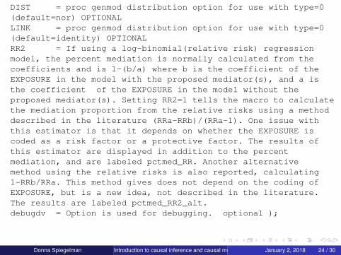
DIST = proc genmod distribution option for use with type=0(default=nor) OPTIONALLINK = proc genmod distribution option for use with type=0(default=identity) OPTIONALRR2 = If using a log-binomial(relative risk) regressionmodel, the percent mediation is normally calculated from thecoefficients and is 1-(b/a) where b is the coefficient of theEXPOSURE in the model with the proposed mediator(s), and a isthe coefficient of the EXPOSURE in the model without theproposed mediator(s). Setting RR2=1 tells the macro to calculatethe mediation proportion from the relative risks using a methoddescribed in the literature (RRa-RRb)/(RRa-1). One issue withthis estimator is that it depends on whether the EXPOSURE iscoded as a risk factor or a protective factor. The results ofthis estimator are displayed in addition to the percentmediation, and are labeled pctmed_RR. Another alternativemethod using the relative risks is also reported, calculating1-RRb/RRa. This method gives does not depend on the coding ofEXPOSURE, but is a new idea, not described in the literature.The results are labeled pctmed_RR2_alt.debugdv = Option is used for debugging. optional );
Donna Spiegelman Introduction to causal inference and causal mediation analysisJanuary 2, 2018 24 / 30

MD as a mediator for distal BC risk factors (1)
Established risk factors for breast cancer (BC) incidence: history of benignbreast disease, family history, BMI, ...
A different type of risk factor: mammographic density, which is awell-established risk factor. However, it is unknown if
”...mammographic density is an intermediate phenotype or whether BC riskfactors influence BC risk and MD separately”.
(Rice et al., Breast Cancer Res., 2016)
Nested case-control study (within the Nurses’ Health studies) :559 cases and 1727 controls.
Outcome: Binary - BC.
Analysis restricted to post-menopausal women. All exposuresmeasured before the mammography.
Donna Spiegelman Introduction to causal inference and causal mediation analysisJanuary 2, 2018 24 / 30

MD as a mediator for distal BC risk factors (2)
Matching of each case to one or two controls on age, currenthormone therapy use, and variables related to the technicalaspects of the mammography.
Analysis adjusted for: age, current BMI, adolescent somatotypeand technical issues related to the mammography.
Sensitivity analysis for unmeasured confounding has shown that aconfounder needs to be strongly associated with BC (1.8) to makea meaningful change in NIE estimates
Donna Spiegelman Introduction to causal inference and causal mediation analysisJanuary 2, 2018 25 / 30

The SAS macro %mediate call
Sample macro call (effect of BMI on breast cancer incidence, mediatedby mammographic density):
%mediate(data=premen, id=id, exposure=BMI,intermed=pct MD covars=age mam c bmi18 c bbd mam nullippar mam c afbc c menarch c avgadol c readbatch2 readbatch3time1 time3 fast2, intmiss=F, outcome=caco, modprint=t,notes=nonotes, where=, extrav=, procopt=, modopt=,link=logit, dist=bin, type = 0, surv=F);
Macro available on:https://www.hsph.harvard.edu/donna-spiegelman/software/mediate/
Donna Spiegelman Introduction to causal inference and causal mediation analysisJanuary 2, 2018 26 / 30
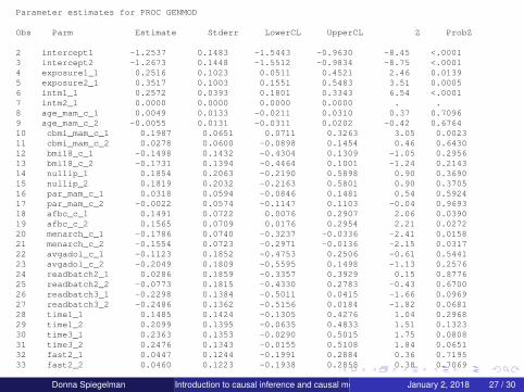
Parameter estimates for PROC GENMOD
Obs Parm Estimate Stderr LowerCL UpperCL Z ProbZ
2 intercept1 -1.2537 0.1483 -1.5443 -0.9630 -8.45 <.00013 intercept2 -1.2673 0.1448 -1.5512 -0.9834 -8.75 <.00014 exposure1_1 0.2516 0.1023 0.0511 0.4521 2.46 0.01395 exposure2_1 0.3517 0.1003 0.1551 0.5483 3.51 0.00056 intm1_1 0.2572 0.0393 0.1801 0.3343 6.54 <.00017 intm2_1 0.0000 0.0000 0.0000 0.0000 . .8 age_mam_c_1 0.0049 0.0133 -0.0211 0.0310 0.37 0.70969 age_mam_c_2 -0.0055 0.0131 -0.0311 0.0202 -0.42 0.676410 cbmi_mam_c_1 0.1987 0.0651 0.0711 0.3263 3.05 0.002311 cbmi_mam_c_2 0.0278 0.0600 -0.0898 0.1454 0.46 0.643012 bmi18_c_1 -0.1498 0.1432 -0.4304 0.1309 -1.05 0.295613 bmi18_c_2 -0.1731 0.1394 -0.4464 0.1001 -1.24 0.214314 nullip_1 0.1854 0.2063 -0.2190 0.5898 0.90 0.369015 nullip_2 0.1819 0.2032 -0.2163 0.5801 0.90 0.370516 par_mam_c_1 0.0318 0.0594 -0.0846 0.1481 0.54 0.592417 par_mam_c_2 -0.0022 0.0574 -0.1147 0.1103 -0.04 0.969318 afbc_c_1 0.1491 0.0722 0.0076 0.2907 2.06 0.039019 afbc_c_2 0.1565 0.0709 0.0176 0.2954 2.21 0.027220 menarch_c_1 -0.1786 0.0740 -0.3237 -0.0336 -2.41 0.015821 menarch_c_2 -0.1554 0.0723 -0.2971 -0.0136 -2.15 0.031722 avgadol_c_1 -0.1123 0.1852 -0.4753 0.2506 -0.61 0.544123 avgadol_c_2 -0.2049 0.1809 -0.5595 0.1498 -1.13 0.257624 readbatch2_1 0.0286 0.1859 -0.3357 0.3929 0.15 0.877625 readbatch2_2 -0.0773 0.1815 -0.4330 0.2783 -0.43 0.670026 readbatch3_1 -0.2298 0.1384 -0.5011 0.0415 -1.66 0.096927 readbatch3_2 -0.2486 0.1362 -0.5156 0.0184 -1.82 0.068128 time1_1 0.1485 0.1424 -0.1305 0.4276 1.04 0.296829 time1_2 0.2099 0.1395 -0.0635 0.4833 1.51 0.132330 time3_1 0.2363 0.1353 -0.0290 0.5015 1.75 0.080831 time3_2 0.2476 0.1343 -0.0155 0.5108 1.84 0.065132 fast2_1 0.0447 0.1244 -0.1991 0.2884 0.36 0.719533 fast2_2 0.0460 0.1223 -0.1938 0.2858 0.38 0.7069
Donna Spiegelman Introduction to causal inference and causal mediation analysisJanuary 2, 2018 27 / 30

Effect for outcome: caco, exposure: HBBDCalculating the proportion of treatment effect mediated by pct_MDAdjusted for: age_mam_c cbmi_mam_c bmi18_c nullip par_mam_cafbc_c menarch_c avgadol_c readbatch2 readbatch3 time1 time3fast2Exposure effect unadjusted for the hypothesized intermediatespct_MD:0.352 ( 0.155 -- 0.548)Exposure effect adjusted for the hypothesized intermediatespct_MD:0.252 ( 0.051 -- 0.452)Proportion of HBBD effect mediated bypct_MD:PTE = 28.459% ( 8.949% -- 47.969%) p = 0.0042
Donna Spiegelman Introduction to causal inference and causal mediation analysisJanuary 2, 2018 27 / 30

Risk factor β̂? (R̂Rtotal) p-value β̂ (R̂Rdirect)
HBBD 0.35 (1.42) < 0.001 0.25 (1.28)BC family history 0.42 (1.52) 0.01 0.42 (1.52)
BMI (age 18) -0.23 (0.79) 0.02 -0.05 (0.95)Age at first birth 0.15 (1.17) 0.03 0.15 (1.16)
Age at menarche -0.16 (0.86) 0.03 -0.18 (0.84)BMI (age18): per 5 units increase; Age at first birth: per 5 years increase;
Age at menarche: per 2 years increase
Risk factor M̂P CI95%p-value
MP test NIE testHBBD 0.28 0.09–0.48 0.004 < 10−6
BC family history 0.004 -0.10–0.11 0.94 0.94BMI (age 18) 0.78 0.06–1.50 0.03 < 10−7
Age at first birth 0.03 -0.09–0.15 0.31 0.30Age at menarche -0.16 -0.36–0.04 0.12 0.04
HBBD: History of benign breast disease
Donna Spiegelman Introduction to causal inference and causal mediation analysisJanuary 2, 2018 28 / 30
Discussion
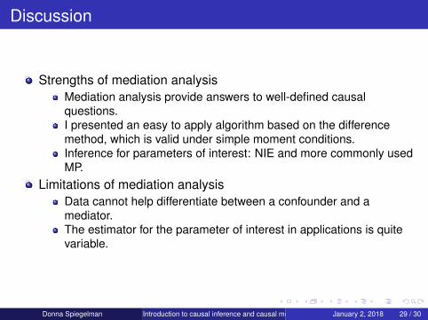
Strengths of mediation analysisMediation analysis provide answers to well-defined causalquestions.I presented an easy to apply algorithm based on the differencemethod, which is valid under simple moment conditions.Inference for parameters of interest: NIE and more commonly usedMP.
Limitations of mediation analysisData cannot help differentiate between a confounder and amediator.The estimator for the parameter of interest in applications is quitevariable.
Donna Spiegelman Introduction to causal inference and causal mediation analysisJanuary 2, 2018 29 / 30
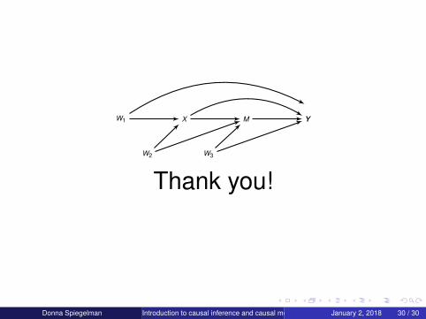
W1 X
W2
M
W3
YY
Thank you!
Donna Spiegelman Introduction to causal inference and causal mediation analysisJanuary 2, 2018 30 / 30

Baron, R. M. and Kenny, D. A. (1986). The moderator–mediator variable distinction insocial psychological research: Conceptual, strategic, and statistical considerations.Journal of personality and social psychology, 51(6):1173.
Pearl, J. (2001). Direct and indirect effects. In Proceedings of the seventeenthconference on uncertainty in artificial intelligence, pages 411–420. MorganKaufmann Publishers Inc.
Robins, J. M. and Greenland, S. (1992). Identifiability and exchangeability for directand indirect effects. Epidemiology, pages 143–155.
VanderWeele, T. J. and Vansteelandt, S. (2010). Odds ratios for mediation analysis fora dichotomous outcome. American journal of epidemiology, 172(12):1339–1348.
Nevo D., Liao X. and Spiegelman D. (2017). Estimation and inference for themediation proportion. To appear in International Journal of Biostatistics
Donna Spiegelman Introduction to causal inference and causal mediation analysisJanuary 2, 2018 30 / 30
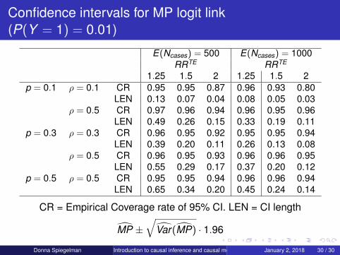
Confidence intervals for MP logit link(P(Y = 1) = 0.01)
E(Ncases) = 500 E(Ncases) = 1000RRTE RRTE
1.25 1.5 2 1.25 1.5 2p = 0.1 ρ = 0.1 CR 0.95 0.95 0.87 0.96 0.93 0.80
LEN 0.13 0.07 0.04 0.08 0.05 0.03ρ = 0.5 CR 0.97 0.96 0.94 0.96 0.95 0.96
LEN 0.49 0.26 0.15 0.33 0.19 0.11p = 0.3 ρ = 0.3 CR 0.96 0.95 0.92 0.95 0.95 0.94
LEN 0.39 0.20 0.11 0.26 0.13 0.08ρ = 0.5 CR 0.96 0.95 0.93 0.96 0.96 0.95
LEN 0.55 0.29 0.17 0.37 0.20 0.12p = 0.5 ρ = 0.5 CR 0.95 0.95 0.94 0.96 0.96 0.94
LEN 0.65 0.34 0.20 0.45 0.24 0.14
CR = Empirical Coverage rate of 95% CI. LEN = CI length
M̂P ±√
V̂ar(M̂P) · 1.96
Donna Spiegelman Introduction to causal inference and causal mediation analysisJanuary 2, 2018 30 / 30

Extras: The Kenny and Baron mediation approach
The traditional approach (Baron and Kenny, 1986) (cited about 63ktimes!) suggested the following series of models and strategy formediation analysis
E(Y |X ,M,W ) = β0 + β1X + β2M (1)E(M|X ,W ) = γ0 + γ1X (2)
E(Y |X ) = β?0 + β?1X (3)
Establish an association between M and X in (2).Establish an association between Y and X in (3).Establish an association between Y and M in (1).
Donna Spiegelman Introduction to causal inference and causal mediation analysisJanuary 2, 2018 30 / 30

Extras: the controlled direct effect
The controlled direct effect
CDE(x , x ′,m) = E(Y (x ′,m))− E(Y (x ,m))
The effect of changing (modifying, intervening on) X = x to X = x ′
while fixing the mediator to a prespecified value m.Relevant when such joint interventions are feasible.CDE(m) is identified under assumptions I + II.Identified under less assumptions (only (I) and (II) are needed).
Robins and Greenland (1992); Pearl (2001)
Donna Spiegelman Introduction to causal inference and causal mediation analysisJanuary 2, 2018 30 / 30

DAGs NP-SEM
In the following DAG, W is a confounder, and the X -Y relationship isconfounded.
W X YY
Markovian assumption: Every variable on the DAG is independentof its non descendants given its parents.Nonparametric Structural Equation Modeling (NP-SEM): Eachnode (variable) on the graph is coupled with a function and arandom variable in the following way:
W = fW (εW )X = fX (W , εX )Y = fY (W ,X , εY )εW , εX and εY are independent.
Go Back
Donna Spiegelman Introduction to causal inference and causal mediation analysisJanuary 2, 2018 30 / 30

Extras: on mediation analysis with confounders
W1 X
W2
M
W3
YY
Let W = {W1,W2,W3} and consider the following set of assumptions(I) Y (x ,m) |= X |W for all x and m(II) Y (x ,m) |= M|W ,X for all x and m(III) M(x) |= X |W for all x(IV) Y (x ,m) |= M(x ′)|W for all x , x ′ and m
Go Back
Donna Spiegelman Introduction to causal inference and causal mediation analysisJanuary 2, 2018 30 / 30

Extras: Simulation Design
Simulate X and M from a bivariate normal distribution withcorrelation ρ.
(Binary outcome) Fix β?1 (TE), MP (mediation proportion) andPr(Y = 1) (outcome rate), E(#cases) (number of cases)
(Continuous outcome) Fix β?1 (TE), MP and β0.
Calculate other model parameters: β1 = (1− p)β?1. β2 = MPρ β
?1.
For binary outcome, β0 by solving Pr(Y = 1) = q for the desired q(e.g., q = 0.1).
Simulate Y given X and M using the conditional model.
Donna Spiegelman Introduction to causal inference and causal mediation analysisJanuary 2, 2018 30 / 30
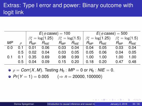
Extras: Type I error and power: Binary outcome withlogit link
E(#cases) = 100 E(#cases) = 500β?1 = log(1.25) β?1 = log(1.5) β?1 = log(1.25) β?1 = log(1.5)
MP ρ RMP RNIE RMP RNIE RMP RNIE RMP RNIE
0.0 0.1 0.01 0.06 0.03 0.04 0.04 0.05 0.03 0.040.5 0.02 0.04 0.03 0.05 0.05 0.06 0.04 0.05
0.1 0.1 0.35 0.69 0.98 0.99 1.00 1.00 1.00 1.000.5 0.04 0.09 0.15 0.20 0.18 0.20 0.47 0.48
ρ = Corr(X ,M). Testing H0 : MP = 0 or H0 : NIE = 0.Pr(Y = 1) = 0.005 (⇒ n = 20000,100000)
Donna Spiegelman Introduction to causal inference and causal mediation analysisJanuary 2, 2018 30 / 30

Extras: The product method and the differencemethod
E(Y |X ,M,W ) = g−1(β0 + β1X + β2M + βT3 W )
E(Y |X ,W ) = g−1(β?0 + β?
1 X + β?3
T W )
E(M|X ,W ) = γ0 + γ1X + γT2 W
The difference method estimates β?1 − β1. The product methodestimates β2γ1.The estimates coincide (algebraically) for the identity link, but notfor other link functions.Variance estimation by bootstrap. Alternatives rely on the deltamethod ignoring the covariance term.If the conditional model is replaced with a model withexposure-mediator interaction,
E(Y |X ,M,W ) = g−1(β0 + β1X + β2M + β3XM + βT4 W ),
there is an extension for the product method available but not forthe difference method.Donna Spiegelman Introduction to causal inference and causal mediation analysisJanuary 2, 2018 30 / 30


![Bayesian Causal Inference - uni-muenchen.de...from causal inference have been attracting much interest recently. [HHH18] propose that causal [HHH18] propose that causal inference stands](https://img.pdfslide.net/doc/110x75/5ec457b21b32702dbe2c9d4c/bayesian-causal-inference-uni-from-causal-inference-have-been-attracting.jpg)