INTRODUCTION TO COMMUNICATION SYSTEMS AND …

5

Chapter 1.

INTRODUCTION TO COMMUNICATION SYSTEMS

AND INFORMATION THEORY

The notion of communication can be described simply as the transmission of information from a given source to a particular destination through a succession of processing stages. This is accomplished by sending an information bearing message as electromagnetic, pulse, or optical energy through vacuum, air, wire, or strands of glass and plastic fiber. Advances in communication systems, computers, high-speed information networks, microelectronics, and multimedia systems have made it possible to send messages over great distances easily, reliably, and most importantly, economically. They have also made it possible to send large amounts of data, both natural and man-made, quickly from one point to another with a very small probability of error.

The very first form of information electrically transferred was telegraphy based on encoding messages using Morse code, which has consisted of sequences of dashes and dots to represent characters in the alphabet. Local telephony followed that. However, people had a natural desire and need to rapidly communicate between distances. Yet, another need was to communicate with more than one user at a time as in the case of broadcasting services. As these goals became reality one after the other, new and large volume information transmission needs emerged.

However, the way we communicate and even we do business has drastically changed during the last twenty years. This is generally attributed to the emergence of transistor technology followed by VLSI, widespread and low-cost computers, high-speed digital networks, and application-specific digital signal processing devices and systems, and sound computational algorithms to aggressively compress everyday signals in various forms. These include voice, audio, video, imagery, radar, sonar, various telemetry, electronic funds transfer, and biofeedback signals. The field of communication science and engineering is even more dynamic these days with the impact of cellular and wireless communication applications, with advancing technology constantly making new equipment and services possible or allowing improvement of the old systems or deploying new services over existing communication facilities.

The rapid deployment of low-cost, modular, and practical communication systems linking the entire globe and the even the outer space up-to-a-point has simulated a plosive growth of complex technical, educational, economical, commercial, and social activities. The cause and effect relationship of this growth had had a snowballing effect on the growth of communication, computer and software industries with no end in sight for foreseeable future. Perhaps, the importance of all of this can be best described by labeling the Twenty-First Century as the Age of Information Technologies --declaration of the International Telecommunication Union of the United Nations—and it is proving to be that way even in the first year of the Third Millennium.

The key blocks common to all communication systems are the information source, transducer, transmitter, channel or the transmission medium, receiver, output transducer, user, and degradation due to various noises and the distortion as depicted in the next section.

© Hüseyin Abut, August 2006

6

1.1 DEFINITIONS AND TERMINOLOGY

In the next few sections, we will define the terminology used in this book and introduce the key concepts with everyday examples. The proper description and a detailed analysis will be presented in later chapters throughout the book. First, we will try to set the framework of this scientific discipline with a generic block diagram of communication system used in many different applications as depicted in Figure 1.1.

Figure 1.1 Block diagram of a generic communication system

Almost all communication systems share a number of common elements. It is common practice to discuss those with a simplified block diagram, frequently attributed to Shannon’s information theoretic presentation of Figure 1.2. Let us now discuss each of these blocks in detail.

Figure 1.2 Block diagram of an end-to-end single user communication system

Information: Set of symbols generated by a person or a system that wants to send them across a transmission medium to another person or a system through electronic means. These include speech, audio signal; Image and video feeds; telemetry and other sensor data; computer bit streams and words.


7

Information Source: To transmit information using electronic means we must convert them into a set of electrical signals and transmit their electromagnetic energy from a sender to the intended user. Electromagnetic energy can travel in various modes: as a voltage or current, as radio waves or as light. For instance, a CCD camera is used for converting optical visual messages into video signals. This step is called the data acquisition process. It is also known as the transducer in classical communication electronics terminology.

Signal: Broadly defined as any physical quantity that varies as a function of time and/or space and has the ability to convey information.

)(tx

- x : the dependent variable (Voltage, picture intensity, pressure, etc. - t : the independent variable (time, space for imagery, etc.).

We can classify signals into four categories according to their appearance in the time-domain. (i) Analog or continuous signals (ii) Discrete-time, (the amplitudes could be non-discrete or discrete) (iii) Discrete-amplitude, where the time-stamp could be continuous or discrete. (iv) Digital. Both input and the output signals are completely discretized and most often mapped

into a sequence of binary numbers }.1,0{For all modes of transmission, the basic laws of physics apply to the selected signal set. The simplest and most important of these laws relates the wavelength ),(λ the velocity and the

frequency Wavelength (m) is the distance between peaks of the oscillations of energy wave or simply, the distance traveled in the time to complete one full cycle; the velocity (m/s) is the speed at which the energy travels through the wire, air, vacuum, or optical fiber, and the frequency (Hz) is the number of oscillations or cycles per second. They are related through:

),(v).( f

fv /=λ (1.1)

Example 1.1: What is the wavelength of a signal in vacuum for a frequency of 1.0 MHz?

(1.2) metersxfv 300100.1/000,000,300/ 6 ===λ

System: A physical entity that operates on a set of primary signals (the inputs) to produce a corresponding set of resultant signals (the outputs). Operations, or processing, may take several forms: modification, combination, decomposition, filtering, extraction of parameters, etc. Systems are normally represented mathematically as a transformation between two signal sets:

21 ]}[{][][ SnxTnySnx ∈=⇒∈ (1.3)

where is the input signal from an allowed set and 1][ Snx ∈ 1S }{•T is a mapping rule between the

input and the output (response) of the system in a range . Generic system model for this behavior is shown in Figure 1.3 embraces all possible combinations of the input/output signal pairs.

][ny 1S


8

Figure 1.3 Generic System Model and Classifications.

Example 1.2: Representations of a speech segment, its samples are shown in Figure 1.4. Similarly, an image frame “Lena” and the details of the left eye region are shown in Figure 1.5.

Figure 1.4 First 5.0 ms segment of the word “information” spoken by a male speaker and its sampled version at a rate 1000 per second.

Figure 1.5 Digitized image “Lena” (8-bits=256 levels and zoom into the left eye.

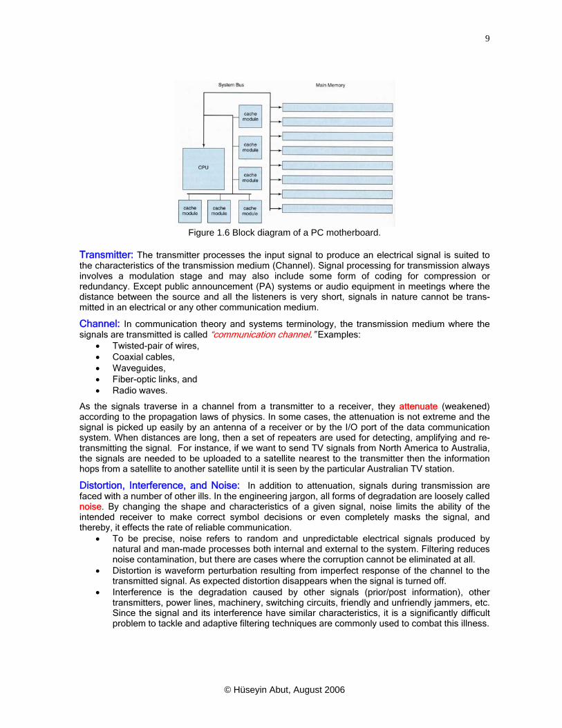
Example 1.3: Wavelets on a computer bus during a data transfer operation between a hard-disk subsystem and the CPU as .shown in Figure 1.6.


9

Figure 1.6 Block diagram of a PC motherboard.

Transmitter: The transmitter processes the input signal to produce an electrical signal is suited to the characteristics of the transmission medium (Channel). Signal processing for transmission always involves a modulation stage and may also include some form of coding for compression or redundancy. Except public announcement (PA) systems or audio equipment in meetings where the distance between the source and all the listeners is very short, signals in nature cannot be trans-mitted in an electrical or any other communication medium.

Channel: In communication theory and systems terminology, the transmission medium where the signals are transmitted is called “communication channel.” Examples:

• Twisted-pair of wires, • Coaxial cables, • Waveguides, • Fiber-optic links, and • Radio waves.

As the signals traverse in a channel from a transmitter to a receiver, they attenuate (weakened) according to the propagation laws of physics. In some cases, the attenuation is not extreme and the signal is picked up easily by an antenna of a receiver or by the I/O port of the data communication system. When distances are long, then a set of repeaters are used for detecting, amplifying and re-transmitting the signal. For instance, if we want to send TV signals from North America to Australia, the signals are needed to be uploaded to a satellite nearest to the transmitter then the information hops from a satellite to another satellite until it is seen by the particular Australian TV station.

Distortion, Interference, and Noise: In addition to attenuation, signals during transmission are faced with a number of other ills. In the engineering jargon, all forms of degradation are loosely called noise. By changing the shape and characteristics of a given signal, noise limits the ability of the intended receiver to make correct symbol decisions or even completely masks the signal, and thereby, it effects the rate of reliable communication.

• To be precise, noise refers to random and unpredictable electrical signals produced by natural and man-made processes both internal and external to the system. Filtering reduces noise contamination, but there are cases where the corruption cannot be eliminated at all.

• Distortion is waveform perturbation resulting from imperfect response of the channel to the transmitted signal. As expected distortion disappears when the signal is turned off.

• Interference is the degradation caused by other signals (prior/post information), other transmitters, power lines, machinery, switching circuits, friendly and unfriendly jammers, etc. Since the signal and its interference have similar characteristics, it is a significantly difficult problem to tackle and adaptive filtering techniques are commonly used to combat this illness.


10

Receiver: Attempts to undo the modifications made at the transmitter and combat degradations took place during transmission, which include: attenuation, distortion, delays, intersymbol and interchannel interferences, echoes, and noise.

Destination: Received electrical signal is converted back to a message form, mostly the original input message category sent by the source to the user, such as a replica of the speaker’s voice in the ear-piece of the user telephone.

User: Intended user of the message sent receives usually a replica of the original message. Transmitted voice, image, video, or data However, the message coming to a user may not be an close replica of the sender’s information. For instance, the access control of a safe room by voiceprint of a legitimate/imposter user is an example to this type of communication. At the end of the speaker verification process, either he/she is given the access or denied. In other words, a single bit instruction to the door lock is the final message.

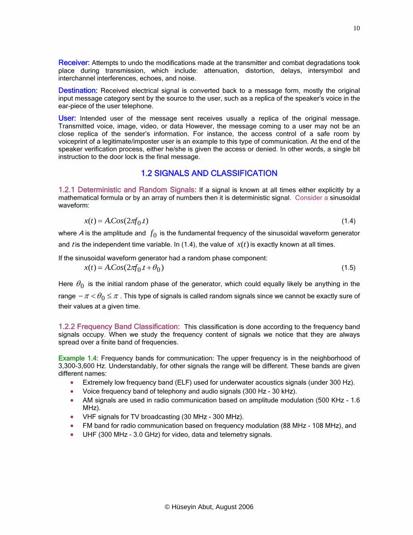
1.2 SIGNALS AND CLASSIFICATION 1.2.1 Deterministic and Random Signals: If a signal is known at all times either explicitly by a mathematical formula or by an array of numbers then it is deterministic signal. Consider a sinusoidal waveform:

).2(.)( 0 tfCosAtx π= (1.4)

where A is the amplitude and is the fundamental frequency of the sinusoidal waveform generator

and t is the independent time variable. In (1.4), the value of is exactly known at all times. 0f

)(tx

If the sinusoidal waveform generator had a random phase component: ).2(.)( 00 θπ += tfCosAtx (1.5)

Here 0θ is the initial random phase of the generator, which could equally likely be anything in the

range πθπ ≤<− 0 . This type of signals is called random signals since we cannot be exactly sure of

their values at a given time.

1.2.2 Frequency Band Classification: This classification is done according to the frequency band signals occupy. When we study the frequency content of signals we notice that they are always spread over a finite band of frequencies. Example 1.4: Frequency bands for communication: The upper frequency is in the neighborhood of 3,300-3,600 Hz. Understandably, for other signals the range will be different. These bands are given different names:

• Extremely low frequency band (ELF) used for underwater acoustics signals (under 300 Hz). • Voice frequency band of telephony and audio signals (300 Hz - 30 kHz). • AM signals are used in radio communication based on amplitude modulation (500 KHz - 1.6

MHz). • VHF signals for TV broadcasting (30 MHz - 300 MHz). • FM band for radio communication based on frequency modulation (88 MHz - 108 MHz), and • UHF (300 MHz - 3.0 GHz) for video, data and telemetry signals.


11

Figure 1.7 Various Frequency-bands used in tele/wireless communication systems. (With permission

from Communication Systems, Carlson, et. Al, Fourth Edition, McGraw-Hill, 1995.) In addition, we have visible light and electromagnetic waves at the high frequency end of the frequency spectrum used in various applications. In all of these signals there is one underlying question:

Is the signal occupying a particular frequency band when it occurs in the nature or is it translated to that specific frequency range from a lower one by a system?

1.2.3 Baseband/Passband Signal Classification:

• If the frequency range where the signal is generated in the nature then is called a baseband signal.


12

• If a signal is translated to another band of frequencies by a man-made system (modulation) or a natural system then we have a passband signal.

Example 1.5: Speech coming out of a public announcement system is a baseband signal, whereas, the signal transmitted by an FM transmitting antenna is a frequency modulated passband signal obtained by heterodyning (mixing) the audio signal with a carrier frequency.

1.2.4: Energy and Power Signals: Signals can be also classified according to their energy and power contents.

• If a signal has a finite energy then it is called an energy signal. • If it attains a finite power value then it is classified as a power signal.

Signals used in communication systems are all power signals, as they will be discussed in the next chapter. 1.2.5 Time Signature Classification:

One of the major classification perspective of signals is according to their behavior as the time progresses. We can classify signals into four categories according to their appearance in the time-domain.

1. Analog or continuous signals 2. Discrete-time, (the amplitudes could be non-discrete or discrete) 3. Discrete-amplitude, where the time-stamp could be continuous or discrete (quantized

signals.) 4. Both input and the output signals are completely discretized and most often mapped into a

sequence of binary numbers (Digital signals) }.1,0{

Deterministic or random analog (continuous Signals): A large portion of information sources in nature is represented by a waveform x(t), where the time stamp t and the amplitude x take on values in a continuous manner. Theoretically both can be in the range{ }∞−∞, . In practice, they are normally constrained by the limitations of physical mechanisms generating them. In analog communication systems, messages and waveforms mentioned above are processed, transmitted, detected and recovered by means of analog devices and inherently they are continuous.

1.2.6 Discrete-Time Continuous-Amplitude (Discrete Signals or Sampled Signals): When analog signals are observed or evaluated at equally spaced discrete time instances, or the observations can take place only at integer time-units, these signals are called discrete-time signals. A clock normally regulates observation times and they are normally periodic. The value of an analog signal is measured or computed at each tick of the clock. The amplitude values have the same restriction as the analog signal, theoretically, the range is the again{ }∞∞− , , but the time instant progresses one

unit at-a-time. In Figure 1.4 a (left), first 5.0 ms of the word “information” spoken by a male speaker is shown. If we measure this information at a rate of 1000 readings per second, the corresponding samples will have amplitude levels as shown in Figure 1.4 b (right).

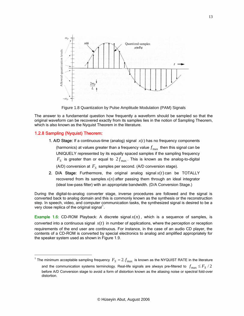
1.2.7 Sampling of Analog Signals (A/D and D/A Conversion): The sampling process provides the link between a continuous (analog) signal and its discrete version. One of the classical examples of discrete-time signals is the sampled outputs of a telephone speech signal passing through an analog-to-digital (A/D) converter, where the waveform is has peak amplitude levels in the range

as shown in Figure 1.9. Let us measure at each clock instant

)(tx{ }+≤≤− PP mtxm )( )(tx :0T

L,2,1,0)()(0

0 === nfornTttxnTX (1.6)

and call these output values samples of . This process is commonly known as the )(tx Pulse Amplitude Modulation (PAM) in the literature as depicted in Figure 1.8.


13

Figure 1.8 Quantization by Pulse Amplitude Modulation (PAM) Signals

The answer to a fundamental question how frequently a waveform should be sampled so that the original waveform can be recovered exactly from its samples lies in the notion of Sampling Theorem, which is also known as the Nyquist Theorem in the literature.

1.2.8 Sampling (Nyquist) Theorem:

1. A/D Stage: If a continuous-time (analog) signal has no frequency components

(harmonics) at values greater than a frequency value then this signal can be

UNIQUELY represented by its equally spaced samples if the sampling frequency is greater than or equal to . This is known as the analog-to-digital

(A/D) conversion at samples per second. (A/D conversion stage).

)(tx

maxf

SF max2 f

SF2. D/A Stage: Furthermore, the original analog signal can be TOTALLY

recovered from its samples after passing them through an ideal integrator (ideal low-pass filter) with an appropriate bandwidth. (D/A Conversion Stage.)

)(tx)(nx

During the digital-to-analog converter stage, inverse procedures are followed and the signal is converted back to analog domain and this is commonly known as the synthesis or the reconstruction step. In speech, video, and computer communication tasks, the synthesized signal is desired to be a very close replica of the original signal1. Example 1.6: CD-ROM Playback: A discrete signal , which is a sequence of samples, is

converted into a continuous signal in number of applications, where the perception or reception

requirements of the end user are continuous. For instance, in the case of an audio CD player, the contents of a CD-ROM is converted by special electronics to analog and amplified appropriately for the speaker system used as shown in Figure 1.9.

)(nx)(tx

1 The minimum acceptable sampling frequency max.2 fFS = is known as the NYQUIST RATE in the literature

and the communication systems terminology. Real-life signals are always pre-filtered to 2/max SFf ≤

before A/D Conversion stage to avoid a form of distortion known as the aliasing noise or spectral fold-over distortion.


14

CD-ROM CD-ROMElectronics Speakers

Figure 1.9 CD-ROM playback systems.

1.2.9 Digital Signals: When the amplitudes of discrete-time samples are limited to then they are both discrete-time and discrete-amplitude signals. These signals are normally represented in terms of binary numbers formed into a sequence of n-bit long codewords. These signals are called “digital signals.” Digital signals can occur in nature as in the case of a PC-motherboard example below or they can be the samples of an analog signal. Common examples to this class are keyboard-to-computer links, inter-board and intra-board communications in computers, parts of satellite communication, emerging communication systems including DSL, digital TV, digital audio, multi-media systems, digital video disk (DVD), network communication, and High Definition TV (HDTV) are some of the systems where the communication is achieved in terms of digital means.

nN 2=

1.3 Quantization and Coding

When an analog signal is sampled into a sequence of PAM signals with amplitudes inside an interval , we can easily turn them into a sequence of binary numbers or codewords by

dividing this range into a finite number of L-levels with a step size of

},{ pp mm −+−

(1.7) Lmv P /2≡ΔNext, we represent each interval by its center point and because there are only L different center

points we can assign one of bits long codewords to every center point. Therefore, we

will need only bits of information for each sample.

)(log2 Lm =)(log 2 Lm =

This step is called:

quantization

and the overall process of sample and hold followed by binary mapping is known as:

Pulse Code Modulation (PCM)

in the community. For instance, an audio signal in Figure 1.10 is first sampled by an A/D converter and held at its sample values until they are transformed into a set of ones and zeros by a quantizer.

Figure 1.10 A simple audio sampling and quantization system.

Example 1.7: m-ary Signals: When we deal with integer only signals, such as, data transfer between a keyboard and the system it is sufficient to use a 2-level pulse set. Suppose that our numbers range between 0 and 15. To transmit each of these 16 different characters we need a sequence of four (4) binary pulses of Figure 1.11.a.


15

However, if we use have 8-level octal pulse set of Figure 1.11b then we will need only two 8-level pulses per decimal number. Similarly, we can expand this octal set (8-level) into the 16-level hexadecimal pulse set by flipping these shapes around the horizontal axis and adding a DC bias. These three different representations are tabulated in Figure 1.12.

Binary 1

Binary 0

0 T 2T0

12

34

56

7

Figure 1.11 Multi-level Signaling. (a) 2-level pulse set; (b) 8-level pulse set.

Decimal Octal Hex Numeral Bit Pattern Decimal Octal Hex Numeral Bit Pattern 0 0 0 0000 8 10 8 1000 1 1 1 0001 9 11 9 1001 2 2 2 0010 10 12 A 1010 3 3 3 0011 11 13 B 1011 4 4 4 0100 12 14 C 1100 5 5 5 0101 13 15 D 1101 6 6 6 0110 14 16 E 1110 7 7 7 0111 15 17 F 1111

Figure 1.12 Decimal, Binary, Octal and Hexadecimal representation

1.3.1 Sampling and Coding Performance Measures (SNR and Transmission Rate): The performance of sampling and coding systems is measured in terms of the rate of transmission in bits per sample or loosely, bit rate in bits per second and the average mean-square difference between the original and its synthesized replica, or more appropriately in terms of a measure called Signal-to-Noise Ratio (SNR) in decibels (dB).

Transmission Rate: Digital signals are generally represented by a set of pair of symbols {1/0; +1/-1; etc.}. However, there will be no loss of generality if an m-ary signal set used. As more and more M-ary logic is used in VLSI devices, systems will shift into the m-ary symbol set. Benefits of this will be enormous in the form of transmission rate reduction, quality, cost, and any combination of these three factors.

For every one of 16 different entries in Figure 1.12, if each pulse lasts seconds and we can represent them with 4-bits then to transmit any number in the range (0,…,15); we will need a rate of transmission:

0T

sBitsTsBitsTmsSampleTR //4////1 000 === (1.8a)

In other words, we have to transmit four consecutive pulses for each sample of message. In the case of an octal pulse set, two (2) consecutive pulse shapes from Figure 1.11b are needed to represent and to transmit these 16 different numbers every second. Then the transmission rate will be: 0T (1.8b) sUnitsOctalTsSampleTR //2//1 00 ==


16

Note that we cannot use the term bits anymore; Octal Units per Second is the official term for this case. Finally, for a hexadecimal pulse set, one of 16 different pulses has to be transmitted at each clock time . 0T The transmission rate is simply:

(1.8c) sHexUnitsTsSampleTR //1//1 00 ==

Signal-to-Noise Ratio (SNR): The most frequently used performance measure in communication systems is the ratio of the signal power to the average mean-square difference between the original signal and its synthesized replica and this is called Signal-to-Noise Ratio (SNR), which is defined by:

NS

PowerNoisePowerSignalSNR =≡ (1.9a)

Typically we express SNR in decibels, that is, (1.9b) dBNSdBSNR )/(log10 10=

Because noise accumulates along a path and the signal attenuates along a path, SNR is always decreasing as the communication distance gets longer and longer.

1.3.2 Analog versus Digital Communication: During the last ten years advances in computers, telecommunications industry and services, and information processing systems and devices have significantly impacted the way we communicate with each other and the way we perform many tasks in our daily lives. This can be attributed greatly to the digital revolution and the explosion in the information dissemination. Digital communication is one of the biggest catalysts of that. This is due to its superiority over analog communication in many ways. Some of these advantages are:

1. In digital communication systems actual signal is not necessary. For instance in binary communication, we only need to know if the signal satisfies the inequality or

. This makes digital systems more robust in comparison to their analog counterparts, where exact tracking of the signal is needed at all times.

2/)( Atx >2/)( Atx <

Example 1.8 Morse Code: A Binary Bit-by-Bit Signaling used in transmitting messages. Let us represent a Mark (logical 1) by the voltage 2/A+ and a space (logical 0) by the voltage . 2/A−

M S M M S S S M 1 0 1 1 0 0 0 1

Figure 1.13 Binary Bit-by-bit Signal Transmission and Channel Degradation

Transmitted Signal Received Signal from Noiseless Channel. Received Signal from Noisy Channel Regenerated Signal at the receiver. Except a time delay it is identical to the original signal.


17

As it can be seen from the Morse code example, a message can be represented in terms of two voltage levels. If the channel is noiseless, then the received signal is simply an attenuated and delayed replica of the original. Even if some noise in the channel affects the signal as shown in (c) it is still possible to recover the original signal with a delay D using a simple threshold level of zero. However, if the noise level is such that the whole shape is drastically changed then the recovered signal may not be a close replica of the original signal. 2. If the distance between the transmitter and receiver is significantly longer than the

recommended values for the particular medium of transmission then regenerative repeaters are needed to achieve reliable communication. In the digital transmission, regenerative repeaters are extremely simple and they get the signal, compare against a threshold level, and reset the signal back to , which eliminates the accumulation of noise along the transmission path.

2/Am

3. Since there are only two levels to represent and transmit a particular message the required circuitry, the design tools, and the test equipment are all simple and low cost. Because of this feature alone, many innovative applications are developed by small entrepreneurial outfits.

4. In digital communication systems, signals from many users can be multiplexed in the time-domain to allocate a given communication channel to more than one user at a given time. For instance, in the North American Digital Telephone Hierarchy (POTS), the digitized samples of 24 voice channels are multiplexed to form a sample rate of 192,000 samples per second, where each voice channel is sampled at a rate of 8,000 sa/s. Furthermore, each sample is quantized into 8-bits long digital words resulting in 1.536 MB/s and an additional 8,000 b/s are employed for framing information. The overall bit rate is 1.544 MB/s. For each of these bits a signal shape is transmitted from one point to another one in the network. At the receiver side each of these bits are demultiplexed to appropriate channels and the voice is synthesized back to analog domain before it is sent to the subscriber’s handset.

In the case of European and international systems, there are 32 channels, 30 of which are dedicated to digitized telephony signals and the remaining two for signaling and other tasks. The overall bit rate is 2.048 MB/s.

5. Once the analog information is converted into bit streams they can be very easily manipulated using one of many encryption strategies whose keys are known only to authorized users. In this way, communications become secure. However, it is extremely difficult to achieve this security in analog systems.

In military communications and civilian emergency services, it is very critical to operate commu-nication without interference from intentional and unintentional jammers. For instance, during a fire or an earthquake, the emergency service messages have to be unquestionably clear and precise. Any intentional and unintentional interference from other communication channels might make a difference between life and death. If these messages are digital they can be easily formed into jammer-proof signals and protected from misuse. In the case of analog emergency services, it is impossible to achieve robustness at similar levels. Intelligence community is full of anecdotal cases of miscommunications and their serious repercussions. Similarly, in financial and securities transactions, the content and the identity of every transaction have to be transmitted over secure channels. With the emergence of e-commerce and e-living this has become extremely critical not only for business community for individual clients as well.

What is the price paid for all of these advantages?

Digital communication systems require larger bandwidth to transmit certain information in comparison with their analog counterparts. However, this is no longer a very critical issue in many places including residential telecommunication services with the fiber-optic links coming to our homes and the availability of low-cost DSL services in many communities.


18

1.4 Principle of Modulation

Usually the information or the message we want to transmit from a source to a distant user requires a channel or a medium of transmission, such as a twisted-pair of wire, a coaxial cable, a microwave link, etc. In these situations, the transmitted signal is attenuates to extremely low levels of power. Then it is necessary to carry the information to a frequency range where the reception will be favorable. To achieve that the signal is modulated to the neighborhood of a carrier frequency Hz,

or equivalently, to radians per second. This process requires some knowledge on Fourier Transforms and its applications, which will be discussed in detail later.

0f0w

X X LPFw0x(t)

Ac.Cos(wct) Ac.Cos(wct)

xDSB(t) xDSB(t) r(t) y(t)

Figure 1.14 Transmitter and receiver operations in Amplitude Modulation (AM).

Amplitude Modulation (AM) is the simplest modulation technique to introduce the topic. As it can be observed from Figure 1.14 the output signal is obtained by multiplying the information bearing signal

with a sinusoidal carrier signal )(tx tfCosA cc π2. , where Ac is the amplitude of the carrier and

cc fw π2= is the radian frequency of the carrier. The output modulated signal is just the product of

the two.

tfCostxAtCoswtxAtx ccccDSB π2).(.).(.)( == (1.10)

We will demonstrate the operation with Matlab tools in the next example.

Matlab Example 1.9: In this example we will be using Matlab Tools to demonstrate the concept of amplitude modulation. Here we assume that:

• Message: and )(tx• Carrier signal: )(tp

are both sinusoidal signals oscillating with two different frequencies. Normally, the message signal will have a lower frequency and the carrier signals will have a much higher one. )(tx

As displayed in Figure 1.15, the output of the modulation is the time-domain product of the message and the carrier information: )().()( txtpty =

In our specific case: • We have chosen a carrier frequency is eight times the tone frequency used as the

message itself. • Two complete cycles of the message tone and sixteen cycles of the carrier and the

modulated output signals are plotted.

Script file (m-file) for implementing this example:


19

% A simple Amplitude Modulation Example: Sinusoidal Tone Modulation % 129 samples of sinusoids are generated as signal and carrier to be modulated n=0:1:128; p=[cos(4*n*pi/16)]; x=[4.0*cos(2*n*pi/64)]; % Plots of the carrier and modulating signal subplot(221),plot(n,p); title('Sinusoidal Carrier Signal'); xlabel('Time'); ylabel('Amplitude'); subplot(222), plot(n,x); title('Message Signal'); xlabel('Time');ylabel('Amplitude'); % Generate the output signal by multiplication y=p.*x; % Plot of the output signal subplot(223),plot(n,y); title('AM Modulated Signal'); xlabel('Time');ylabel('Amplitude')

Figure 1.15 Modulating signal, carrier, and the output waveform of the AM system in Example 1.11.

0 50 100 150-1

-0.5

0

0.5

1Sinusoidal Carrier Signal

Time

Am

plitu

de

0 50 100 150-4

-2

0

2

4Message Signal

Time

Am

plitu

de

0 50 100 150-4

-2

0

2

4AM Modulated Signal

Time

Am

plitu

de


20

Reasons for modulating signals:

1. Efficient Transmission: Signals attenuate according to the propagation characteristics of the channel used. For instance, the most favorable frequency range for a fiber-optic link used for high-speed data communication tasks is significantly different from a short-haul microwave transmission operating at 23-26 GHz. band. Therefore, we modulate signals to the most frequency range for a given channel medium.

2. Hardware Ease: The components used in the electronic circuitry vary significantly as the fre-quency range changes. For instance, a piece of conducting wire acts a distributed RLC circuit in microwave frequencies. On the other hand, we need to use fairly large size components in low frequencies, which make the circuitry big in dimensions. As the current trend of miniaturization continues it is extremely critical to use the available real estate in silicon VLSI device efficiently. Therefore, we modulate signals sometimes to better use the electronics properties of the material we use in the design.

3. Antenna Size: For efficient radiation of electromagnetic energy, which we use to transmit signals, the transmitter and receiver antennas should be on the order of one-tenth or more of the wavelength of the signal transmitted. For most baseband signals, such as voice and audio, the wavelengths are on the order of 100-300 Km. In this case, if we want to transmit audio signals in the atmosphere without any modulation the dimensions of the transmitter and receiver antennas need to be unacceptably large (larger than a tennis court!) On the other hand, the antenna size of an FM radio, which is operating in 88.0 108.0 MHz. is on the order of 30 cm.

4. Reduced Noise/Interference: Every communication channel is subject to environmental, device, and man-made noises and interference. For instance, the radiating waves in TV broadcasting would be affected to the level of unacceptability by the humidity in the air, the clouds, the wind, and the cosmic effects in the sun rays if they were not modulated to the current TV channel frequencies. This is due to the fact that the various levels of the atmosphere have good noise immunity at some frequencies but very poor in many other frequency ranges. Therefore, we modulate signals to favorable frequency bands to gain noise immunity. If we do not modulate the audio signals then the radiating waves will have interference from other speakers in a room since they are all talking at the same frequency band. Furthermore, the signal from interfering speakers will be dominant since their sources are closer.

5. Efficient Spectrum Utilization: Signals from a number of sources can be multiplexed together and the resultant ensemble can be transmitted over a particular channel. Thus a given frequency spectrum is shared by multiple number of users. For instance, 96 voice channels or 4 TV channels are multiplexed in time-domain in the Level 2 of the North American Digital Telephony Hierarchy. In other words, 96 telephone calls take place simultaneously over this communication link. In addition to time-domain multiplexing (TDM), it is also possible to multiplex in the frequency domain (FDM) and code-space domain (CDMA). In all of these schemes a given frequency bandwidth is more efficiently used in comparison with one-channel one pair of users scheme.

6. Frequency Selectivity: Modulating signals to some predefined frequency bands permits users to tune in to many signals at their own choice. Examples are channel surfing on TV or seek and tune in newer radios. TV channels are assigned over and over again in geographically distant locations. Because of this capability only a few number of TV channel frequencies are sufficient to cover even large countries like United States.

1.5 Communication System Resources and Performance Measures

In all communication systems, there are two critical resources and three primary performance evaluation criteria. Channel bandwidth and the transmitter power constitute the primary resources and subjective quality and Signal-to-Noise Ratio (SNR) are the leading performance measures. In the case of digital communications though, the bit error rate (Pe) and the compression factor are also

very important measures. In many applications, they replace SNR completely. In the case of analog


21

signal transmission by means of digital communication systems, yet another measure becomes very important: Signal-to-Quantizing Distortion Ratio (SDR)2.

The transmitter power is defined by the average power of the signal pumped into a given channel. Higher power results in better signal reception at the other end of a particular channel. On the other hand, the bandwidth covers the band of frequencies allocated for the transmission of a given signal. Again systems with higher bandwidth produce better results. Both of these resources are directly proportional to the cost of communication systems. Therefore, a universal objective of all communication systems is to use these two resources as efficiently as possible. In some applications, only one of these two parameters is more critical. Then the goal is to make the system constraint on that parameter. For instance, the communication satellites are power-constrained systems, whereas the communication over an ordinary telephone line is bandwidth constrained. Finally, next generation digital cellular phones will have both power and bandwidth constraints. Therefore, their design and low-cost production are engineering challenge yet to be met.

Communication systems, whose ultimate users are human sensory perception mechanisms, are measured in terms of their subjective performances. However, ratings like excellent, good, average, poor, and unacceptable, etc. is very subjective by their nature. System designers and evaluators pre-fer quantitative yardsticks for ease of comparison. A number of widely accepted measures like Dynamic Rhyme Tests (DRT), A-B comparison tests, Mean Opinion Scores (MOS), and others are developed for speech and image encoding schemes. Even though these measures are more meaningful in many applications, they are very time consuming, costly, and perhaps, most importantly, they can be totally misleading if the test conditions are not tightly controlled. Because of these difficulties quantitative measures are generally used for performance evaluations.

1.5.1 Signal-to-Noise Ratio (SNR): Recalling the definition (1.9) earlier, the most fundamental quantitative performance measure is the Signal-to-Noise Ratio (SNR) defined as the ratio of the average signal power to the RMS value of the channel noise amplitude measured in decibels (dB).

NSSNR = or equivalently, dBNSSNR )/(log*0.10 10= (1.11)

where S and N are is the signal power and the overall noise power, respectively. Understandably, higher the SNR better the system will perform. SNR can be improved either by increasing the signal power, which is not possible in power constrained systems, or by lowering the noise power in the bandwidth of interest. Reducing the latter quantity is almost all the time the primary objective of various encoding, enhancement, and other signal processing schemes. Example 1.10: Compute the SNR for a signal at 10 W and a noise level of 0.5 W.

SNR = 10.0*log10(S/N) =10.0*log10(10/0.5)=13.0 dB

In many systems applications the input signal and its response are expressed in terms of voltage levels. If we assume the input and load resistances are the same we can measure the processing gain, or the circuit gain as it is called in electronics, in terms of dB.

)(log*0.20)(log*0.10 102

2

10in

out

in

outG V

V

V

VP == (1.12)

Example 1.11: A signal input to an amplifier has a peak value 0.1 V and the output is 5.0 V. What is the processing gain?

2In many communication texts and communication industry documents, quantizing distortion is also called quantizing noise and the term SNR is adapted as signal-to-quantizing noise ratio. In this text, we will try to differentiate between the two terms as much as possible to avoid the unavoidable confusion.


22

dBVV

Pin

outG 34)

1.00.5log(*0.20)log(*0.20 ===

System design specifications are often made using dB values and engineers are asked to calculate exact value of the corresponding power, voltage, or magnitude. The conversion formulas for these are given by:

0.1010*GP

inout PP = Watts and 0.2010*GP

inout VV = Volts (1.13)

Example 1.12: Find the output voltage of a transmitter amplifier with a 9.0 dB processing gain if the input signal has 1.6V peak value.

voltsVVGP

inout 509.410*6.110* 209

0.20 ===

Third primary performance measure is the processing delay and it is defined as the total time it takes a particular message generated an information source to reach its intended user’s sensory receptors. Lower the processing delay sooner we will achieve our objective in a given communication system. There are many techniques requiring very little power, almost zero bandwidth and a very large SNR but the processing delay is so large that it makes them totally unacceptable as a viable communication system. One vivid example is to use a messenger pigeon to deliver an emergency message! In digital communication systems, the average probability of bit error Pe or Bit Error Rate (BER) is more important than any other measure. It does not actually make any difference, if the error rate is so high that the transmitted messages and the received ones imply two opposing decisions and leading to wrong commands and disaster in many tasks. One example is to erroneously deny access to a genuine account holder in his bank account or to transfer his funds to somebody else’s account.

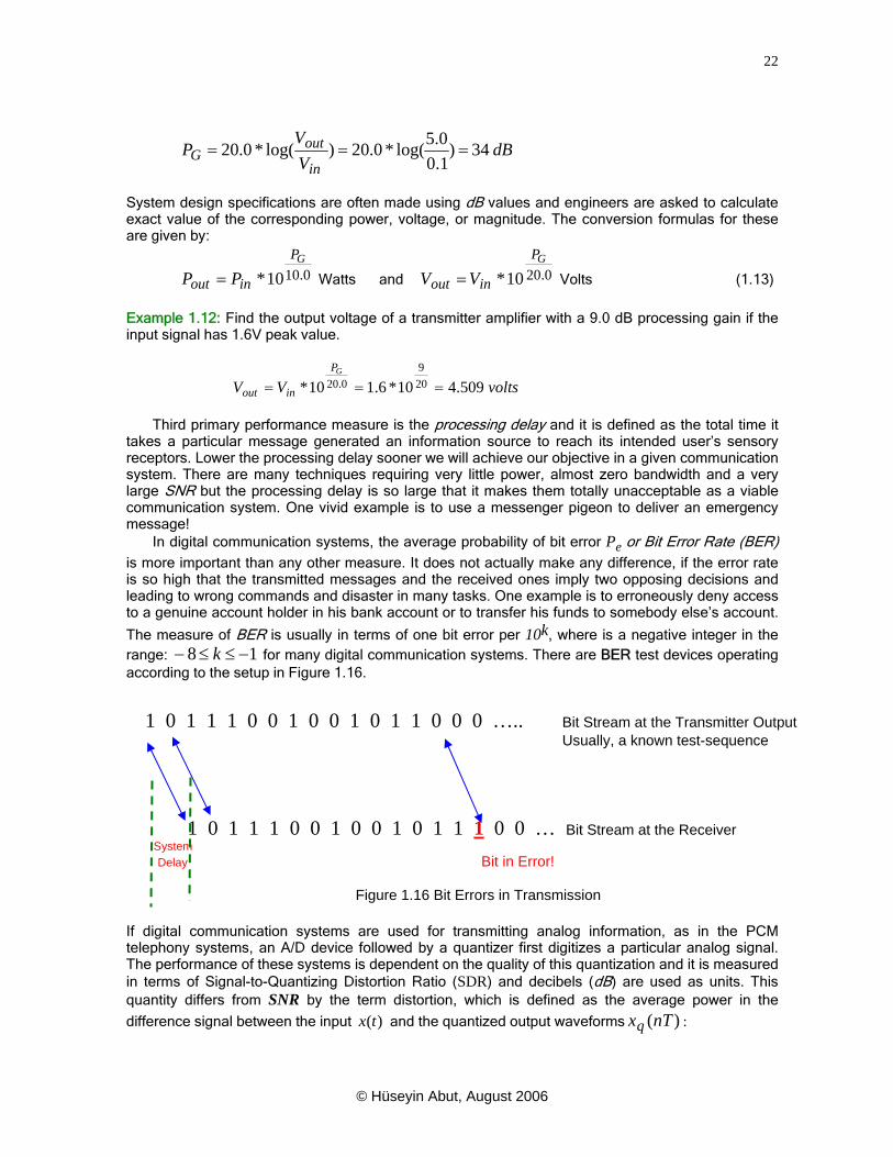
The measure of BER is usually in terms of one bit error per 10k, where is a negative integer in the range: for many digital communication systems. There are BER test devices operating according to the setup in Figure 1.16.

18 −≤≤− k

1 0 1 1 1 0 0 1 0 0 1 0 1 1 0 0 0 ….. Bit Stream at the Transmitter Output Usually, a known test-sequence 1 0 1 1 1 0 0 1 0 0 1 0 1 1 1 0 0 … Bit Stream at the Receiver System Delay Bit in Error!

Figure 1.16 Bit Errors in Transmission

If digital communication systems are used for transmitting analog information, as in the PCM telephony systems, an A/D device followed by a quantizer first digitizes a particular analog signal. The performance of these systems is dependent on the quality of this quantization and it is measured in terms of Signal-to-Quantizing Distortion Ratio (SDR) and decibels (dB) are used as units. This quantity differs from SNR by the term distortion, which is defined as the average power in the

difference signal between the input and the quantized output waveforms : )(tx )(nTxq


23

(1.14) dBDSSDR in )/(log*0.10=

where S and D are the average signal and distortion powers, respectively. If T is the sampling period in the A/D stage and E is the expectation or averaging operator then the distortion power is given by:

(1.15) })]()({[})({ 22 nTxtxEteED q−==

Example 1.13: Find the signal-to-distortion ratio of an L-level uniform quantizer. Let us assume the signal has a peak-to-peak voltage range of Vpp = 2Vp Volts. The peak power of this signal

normalized to: is given by: Ω0.1

wattsqLLqVP PPS 4/)2/()2/(*0.1 2222 ===

where L is the number of quantizer steps as discussed earlier. Since the uniform quantizer has a step size of q Volts each sample of the signal can have an error of not more than q/2 and not less than -q/2. Therefore, degradation of signal is limited to half of a quantizer step: . If we

assume this quantizing distortion or error signal e(t) is uniformly distributed over a single quantizer step size of q volts we can obtain the quantizer error variance by:

voltsq 2/m

12

)]([1 22

2/

2/

qdtteq

Nq

qq =∫=

− (1.16)

When we combine these two equations we obtain the SDR equation for a uniform quantizer with L-levels:

22

22*3

12/4/)( L

qqL

NP

SDRq

S === (1.17)

It is clear from above the signal-to-distortion ratio SDR increases with the square of the number of quantizer levels.

Bandwidth: Bandwidth B of communication systems is defined as the range of frequencies that a channel can transmit information with reasonable fidelity. Depending upon the system and the medium of transmission, the bandwidth can be a few Hertz as in the earthquake, through 1014 Hz in the case of fiber-optic link. But for a given communication channel or the medium of transmission S and B are exchangeable.

Example 1.14: Suppose a communication system is transmitting messages using a thirty-two letter alphabet, L = 32 letters and a binary signaling.

522 == mL which implies we need only m=5 bits to represent every message symbol. In other words, 5 bits are to be transmitted per T0 seconds if one message is generated every T0 seconds. This requires a 5*B Hz. channel bandwidth.

For the same system with L =32, let us employ a 32-ary signaling scheme using the set of symbols: , in which case, there are now 31 threshold levels to distinguish among

32 letters: . Obviously, it will be necessary to increase the signal power in order to get the same accuracy per letter as in the binary signaling case, resulting in an increase in the transmitter signal power. By doing so we need to send a single 32-ary signal every T0 seconds. This corresponds to a reduction by five in channel bandwidth.

]2/31,,2/3,2/[ AAA mLmm

]15,,,0,,,15[ AAAA LL −−

One of the most frequently encountered interpretations of bandwidth is the location of -3dB value. This interpretation is associated with the concept of circuit theory and using RLC circuits as filters, where the bandwidth is defined as the width of the frequency spectrum between two -3dB points of the signal amplitude versus frequency values. It is usually called 3dB down point. In this case, the


24

maximum signal amplitude, regardless of frequency, is accepted as the 0-dB reference, and all other amplitudes at various frequencies are plotted against this reference. Thus, the amplitude values drop to a 3dB down level at the edges of the bandwidth. This can be best illustrated with a RC-network, where the load is assumed as the voltage drop across the capacitor.

Example 1.15: Consider the RC-Filter shown in Figure 1.17:

in C=0.1x10-6 F out

R = 100 KOhms dB

0 --3-6-9

| | | | | f (Hz)5 10 15 20 25

- - -

Figure 1.17 RC-Filter circuit and frequency response.

From the elementary circuit theory, we can write the 3-dB bandwidth of this circuit by:

HzRC

fC 1610.10.2

12

175≅==

−ππ

If a communication system is designed for a bandwidth of B1 and it achieves an SNR1 then it is possible to transmit the same information over another channel with a bandwidth B2 and the required

SNR needs to be:

(1.19) 21 /12 )( BBSNRSNR ≈

The above approximation is used as an upper bound on bandwidth versus SNR trade-off in communi-cation systems.

1.7 Information Theory Bounds on Communication

Performance limitations of communication systems, in particular, the source and the channel issues, are the topics of Information Theory, which applies the laws of probability, spectral estimation, and many other applied mathematics to the study of generation, representation, transmission, and manipulation of information. From the perspective reliable communication systems, it attempts to find answers to:

• Given an information source, how much information it carries, how much redundancy it has, what is the fundamental limit of compression? This area of information theory is known as the Source Coding. Entropy H of a source and the Rate-Distortion R(D) function are the two major notions we study.

• Given a channel subject to noise, echoes, interference, and other degradations, what is the fundamental limit on the transmission rate of information over this channel? This field is called the Channel Coding. The Channel Capacity C and the bit error rate (BER) are the critical concepts addressed here.

Performance bounds on these notions are known as Shannon bounds due to the founding father of information theory. In order to present them, we need to introduce a few concepts. 1.7.1 Self-Information and Entropy: Assume a random source S with capability to generate any one of L different messages, where each of these messages has a probability of occurring: . The self-information of this source is defined by: }1,,1,0;{ −== LkPP kS L

symbolbitsLkforPI kk /1,,1,0)/1(log2 −=≡ L (1.20)


25

Knowledge of self-information is not a very useful measure for random sources since it can vary drastically from a particular outcome to another. On the other hand, the average self-information over all possible outcomes of a given source is known as the Entropy H and it represents the lower bound on compression systems.

symbolbitsP

PSHL

k kk /)1(log.)(

1

02∑≡

−

= (1.21)

Next we will present the Shannon’s first fundamental theorem on coding. Let us assume that a given

source has an alphabet with L different symbols, or equivalently, L different messages, and the kth symbol occurs with probability Pk, k= 0, 1,..., L-1. Let us consider an encoder, which assigns a

codeword with lk bits to a particular symbol sk. The average length of this source coder is simply:

∑=−

=

1

0/.

L

kkk symbolbislPL (1.22)

1.7.2 Shannon Source Coding Theorem: Given a source S with entropy H(S) then it is possible to

encode this source with a distortionless source coder with an average length L provided: )(SHL ≥ (1.23)

Conversely, there is no distortionless source coder to encode S if

)(SHL < (1.24)

In other words, H(S) represents the distortionless coder with the minimum achievable average code length. Similarly, converse statement implies that all coders operating at an average length less than the entropy will have distortion.

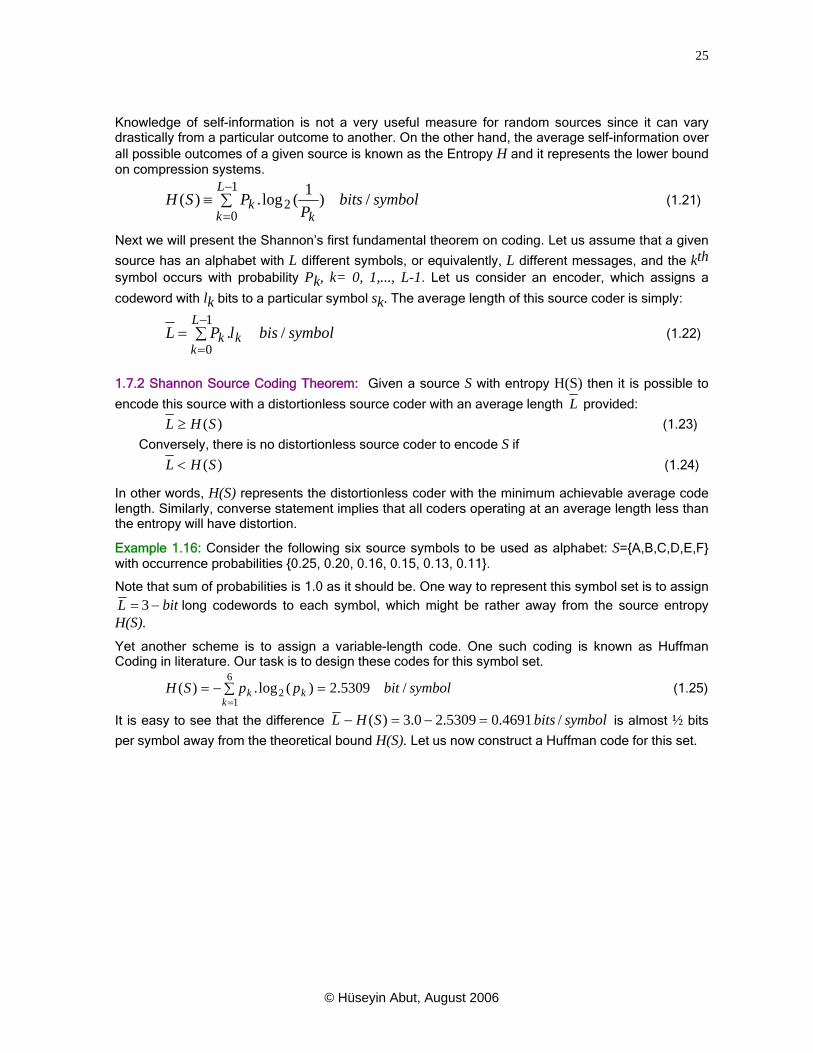
Example 1.16: Consider the following six source symbols to be used as alphabet: S={A,B,C,D,E,F} with occurrence probabilities {0.25, 0.20, 0.16, 0.15, 0.13, 0.11}.

Note that sum of probabilities is 1.0 as it should be. One way to represent this symbol set is to assign bitL −= 3 long codewords to each symbol, which might be rather away from the source entropy

H(S). Yet another scheme is to assign a variable-length code. One such coding is known as Huffman Coding in literature. Our task is to design these codes for this symbol set.

(1.25) symbolbitppSHk

kk /5309.2)(log.)(6

12 =∑−=

=

It is easy to see that the difference symbolbitsSHL /4691.05309.20.3)( =−=− is almost ½ bits

per symbol away from the theoretical bound H(S). Let us now construct a Huffman code for this set.


26

Symbol PkA

B

C

D

E

F

0.25

0.20

01.6

0.15

0.13

0.11

HuffmanCode10

00

111

110

011

010

CodeLength

2

2

3

3

3

3

0

0

0

0

01

1

1

11

0.31

0.24

0.44

0.56

1.0

BinaryCode000

001

010

011

100

101

CodeLength

3

3

3

3

3

3

Figure 1.18 Variable-length (Huffman) Coding example.

The average length of this code is:

symbolbitsxxxxxxLHuffman /55.2311.0313.0315.0316.0220.0225.0 =+++++=

The difference in this case is lowered to:

symbolbitsSHL /0191.05309.255.2)( =−=− , which is almost perfect. 1.7.3 Channel Capacity: Assume a source emits symbols S0,S1,...,SL-1 at a rate R bits per second

and they are transmitted over a channel with a bandwidth B Hz. The receiver detects signals coming from the channel with a signal-to-noise ratio SNR= S/N, where S and N are the signal and noise powers at the input to the receiver, respectively. The receiver emits symbols Y0,Y1,...,YK-1. These

symbols may or may not be identical to the source set depending upon the nature of the

receiver. Furthermore, L and K may be of different size. In other words, some codewords might be totally lost in the channel or the channel itself might add some codewords.

}{ kY }{ kS

If the channel is noiseless then L and K are identical and the receiver symbols are also same as the source symbols. In this case, the reception of some symbol Yk uniquely determines the source

symbol Sk. In the noisy channels, however, there is a certain amount of uncertainty regarding the

identity of the transmitted symbol when Yk is received.

Shannon showed that the capacity of such noisy channel is defined as follows: If the information channel has a bandwidth of B Hz. and the system is designed to operate at a signal-to-noise ratio SNR then the highest rate we can reliably transmit binary information is: ondbitsSNRBC sec/)1(log. 2 += (1.26) 1.7.4 Shannon Channel Coding Theorem: Given a channel with a capacity C, it is possible to transmit symbols from a source emitting at a rate R bits per second with an arbitrarily small probability of error in over this channel if Conversely, all systems transmit at a rate R such that are bound to have errors with probability one.

.RC ≥RC <


27

This implies that we can have good source coders; even perfect ones, if the source rate is under the channel capacity. We may not be able design such good coder but that is our problem, not the information theory’s! On the other hand, all coders are destined to make errors if they operate at a rate above the channel capacity. Since the middle of nineteen seventies scientists and engineers working in the fields of information theory and its applications to modern communication systems have been regularly coming up with sound coding algorithms and their clever real-time implementations and the gap between Shannon bounds and actual values have been narrowing. Because this phenomenon, we have been observing exciting developments in the field of telecommunications for some time now.


Documents

INTRODUCTION TO COMMUNICATION SYSTEMS AND …