Introduction to Computer

Graphics4. Viewing in 3D

National Chiao Tung Univ, Taiwan

By: I-Chen Lin, Assistant Professor

Textbook: E.Angel, Interactive Computer Graphics, 5th Ed., Addison Wesley

Ref: Hearn and Baker, Computer Graphics, 3rd Ed., Prentice Hall

Outline

Classical views

Computer viewing

Projection matrices

Classical Viewing

Viewing requires three basic elements

One or more objects

A viewer with a projection surface

Projectors that go from the object(s) to the projection surface

Each object is assumed to constructed from flat principal faces

Buildings, polyhedra, manufactured objects

Planar Geometric Projections

Standard projections project onto a plane.

Projectors are lines that either

converge at a center of projection

are parallel

Such projections preserve lines

but not necessarily angles

When do we need non-planar projections?

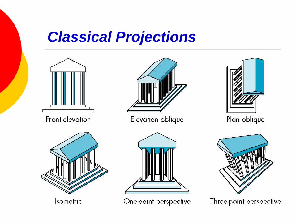
Classical Projections

Perspective vs Parallel

Classical viewing developed different techniques for drawing each type of projection

Mathematically parallel viewing is the limit of perspective viewing

Computer graphics treats all projections the same and implements them with a single pipeline

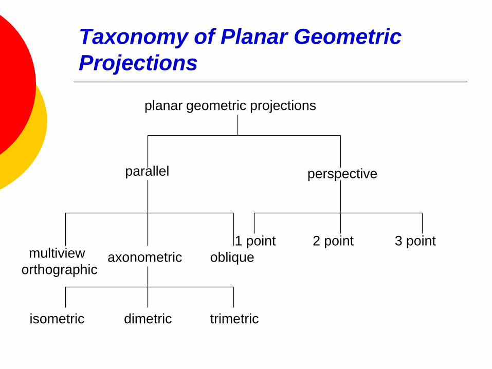
Taxonomy of Planar Geometric

Projections

parallel perspective

axonometricmultiview

orthographicoblique

isometric dimetric trimetric

2 point1 point 3 point

planar geometric projections

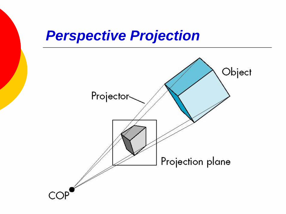
Perspective Projection

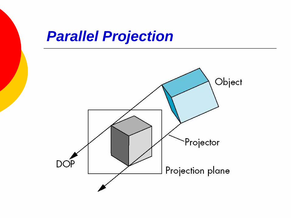
Parallel Projection

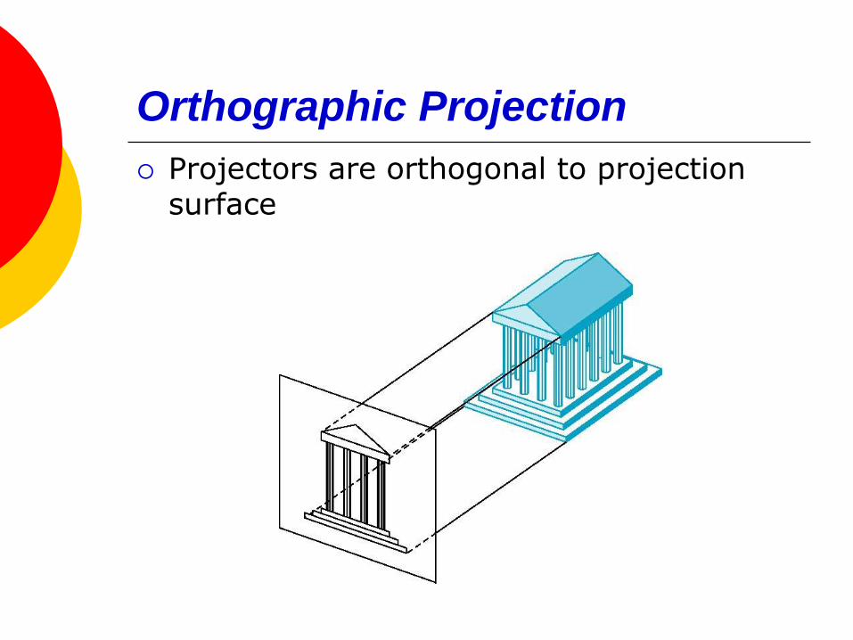
Orthographic Projection

Projectors are orthogonal to projection surface

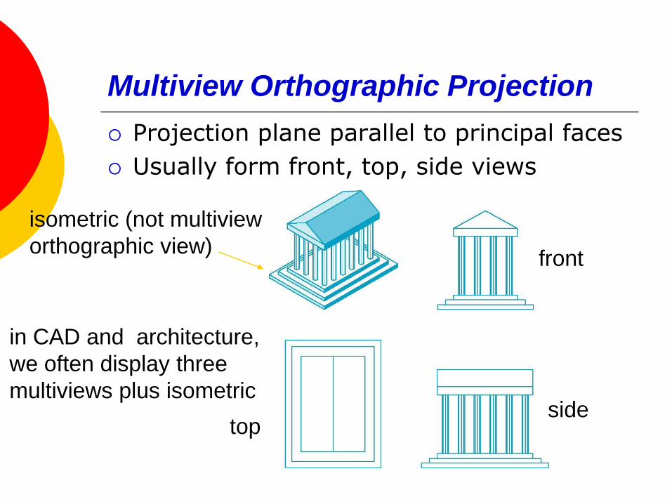
Multiview Orthographic Projection

Projection plane parallel to principal faces

Usually form front, top, side views

isometric (not multiview

orthographic view)front

sidetop

in CAD and architecture,

we often display three

multiviews plus isometric

Advantages and Disadvantages

Preserves both distances and angles

Shapes preserved

Can be used for measurements

Building plans

Manuals

Cannot see what object really looks like because many surfaces hidden from view

Often we add the isometric

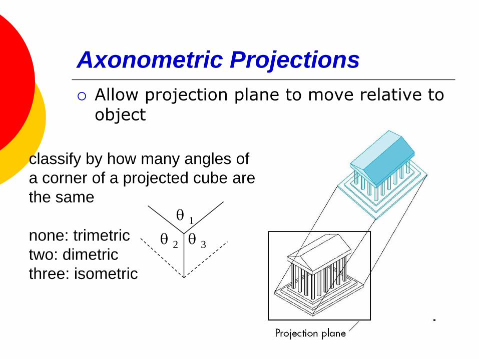
Axonometric Projections

Allow projection plane to move relative to object

classify by how many angles of

a corner of a projected cube are

the same

none: trimetric

two: dimetric

three: isometric

q 1

q 3q 2

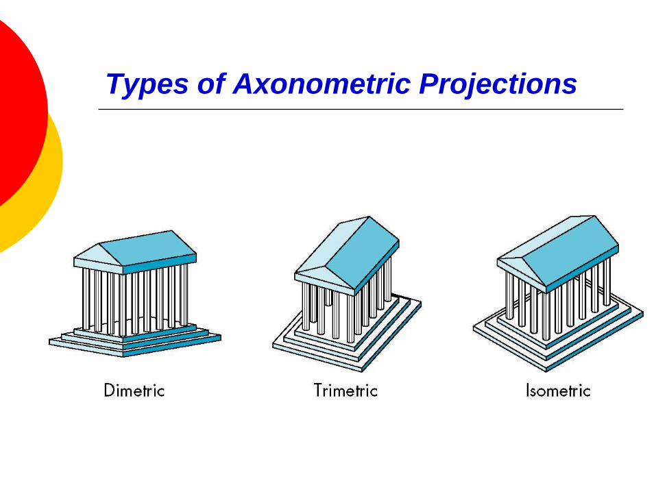
Types of Axonometric Projections

Advantages and Disadvantages

Lines are scaled (foreshortened) but can find scaling factors

Lines preserved but angles are not Projection of a circle in a plane not parallel to

the projection plane is an ellipse

Does not look real because far objects are scaled the same as near objects

Used in CAD applications

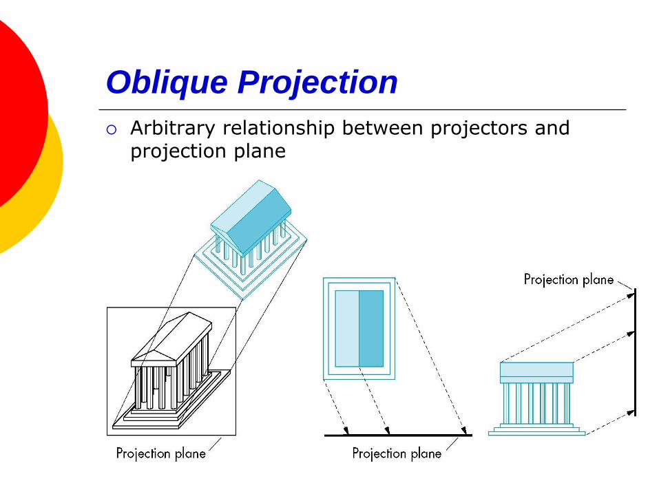
Oblique Projection

Arbitrary relationship between projectors and projection plane

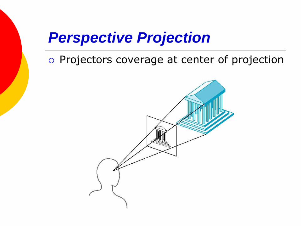
Perspective Projection

Projectors coverage at center of projection

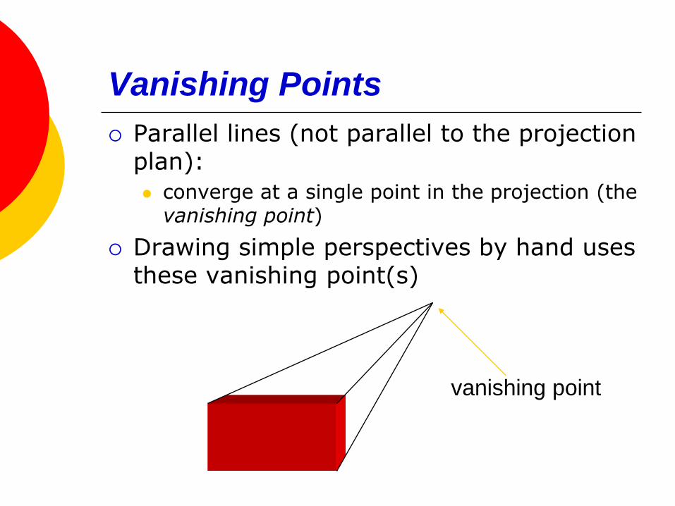
Vanishing Points

Parallel lines (not parallel to the projection plan):

converge at a single point in the projection (the vanishing point)

Drawing simple perspectives by hand uses these vanishing point(s)

vanishing point

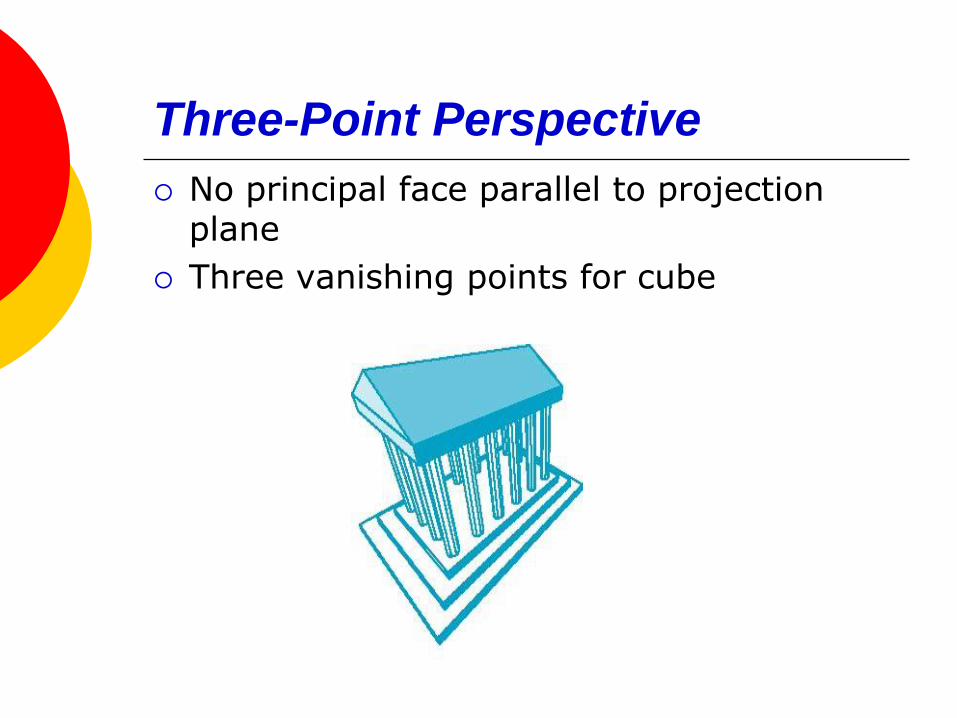
Three-Point Perspective

No principal face parallel to projection plane

Three vanishing points for cube

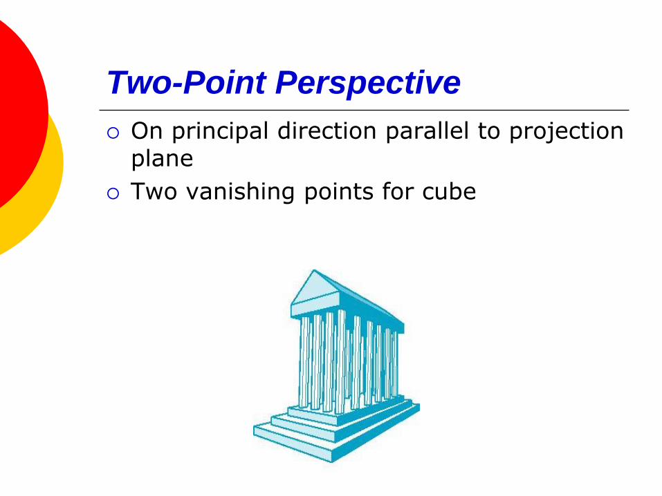
Two-Point Perspective

On principal direction parallel to projection plane

Two vanishing points for cube

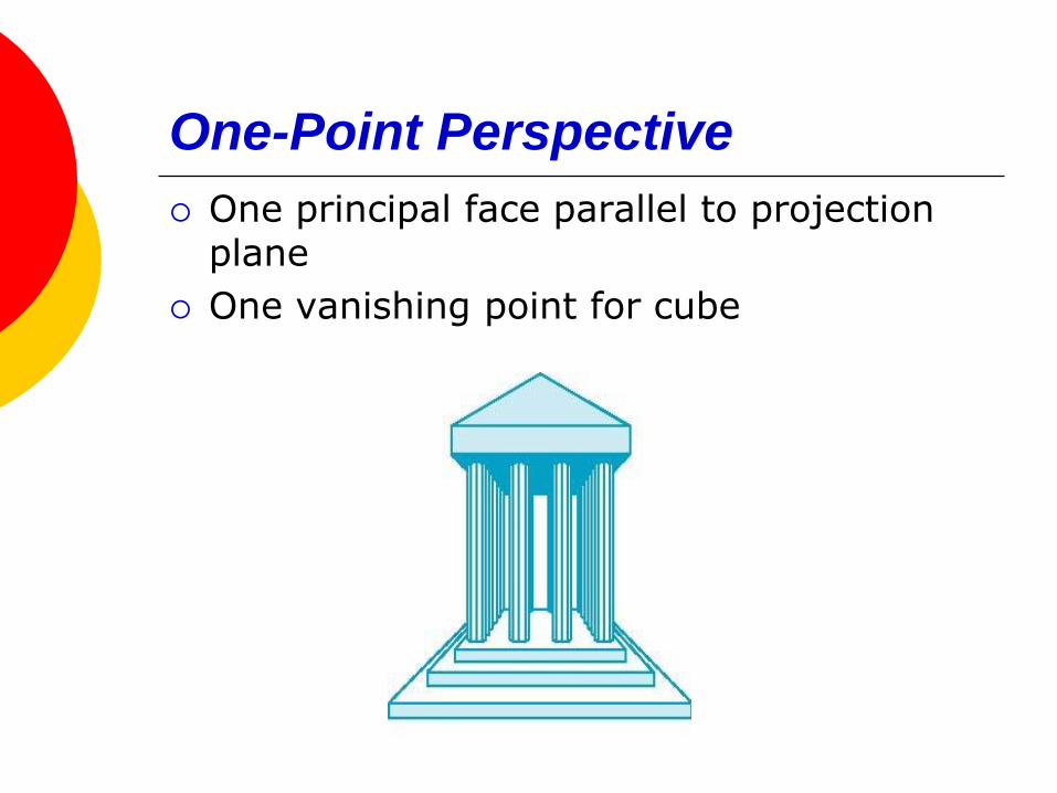
One-Point Perspective

One principal face parallel to projection plane

One vanishing point for cube

Advantages and Disadvantages

Diminution: Objects further from viewer are projected

smaller (Looks realistic)

Nonuniform foreshortening: Equal distances along a line are not projected

into equal distances

Angles preserved only in planes parallel to the projection plane

More difficult to construct by hand than parallel projections

Projections and Normalization

The default projection in the eye (camera) frame is orthogonal

For points within the default view volume

xp = x

yp = y

zp = 0

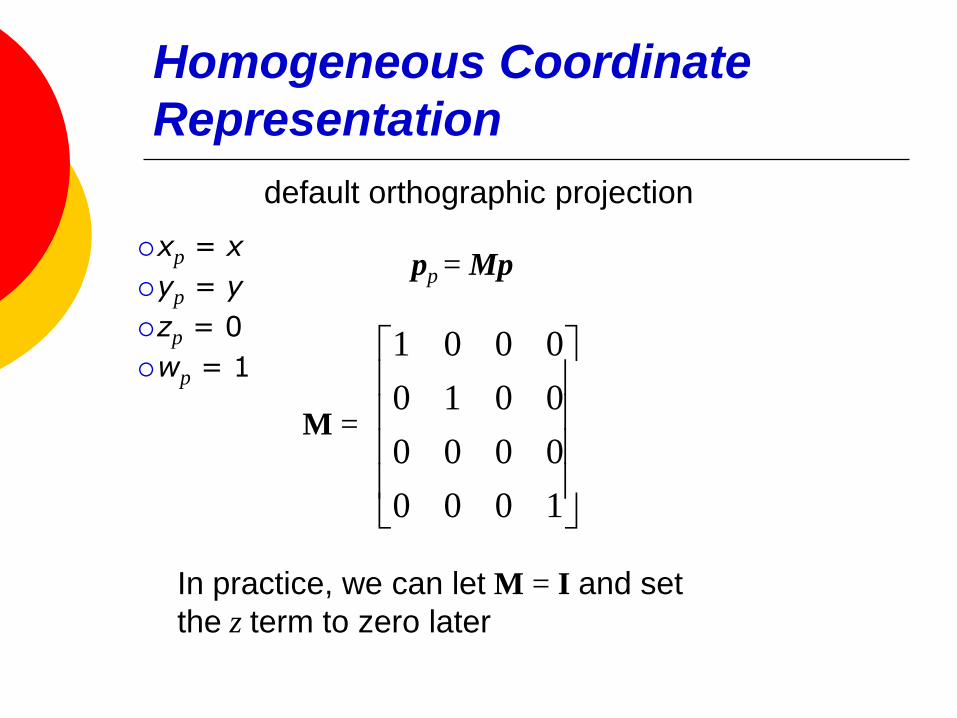
Homogeneous Coordinate

Representation

xp = x

yp = y

zp = 0

wp = 1

pp = Mp

M =

1000

0000

0010

0001

In practice, we can let M = I and set

the z term to zero later

default orthographic projection

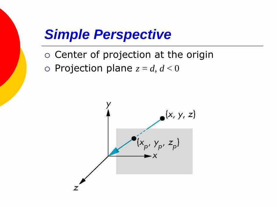
Simple Perspective

Center of projection at the origin

Projection plane z = d, d < 0

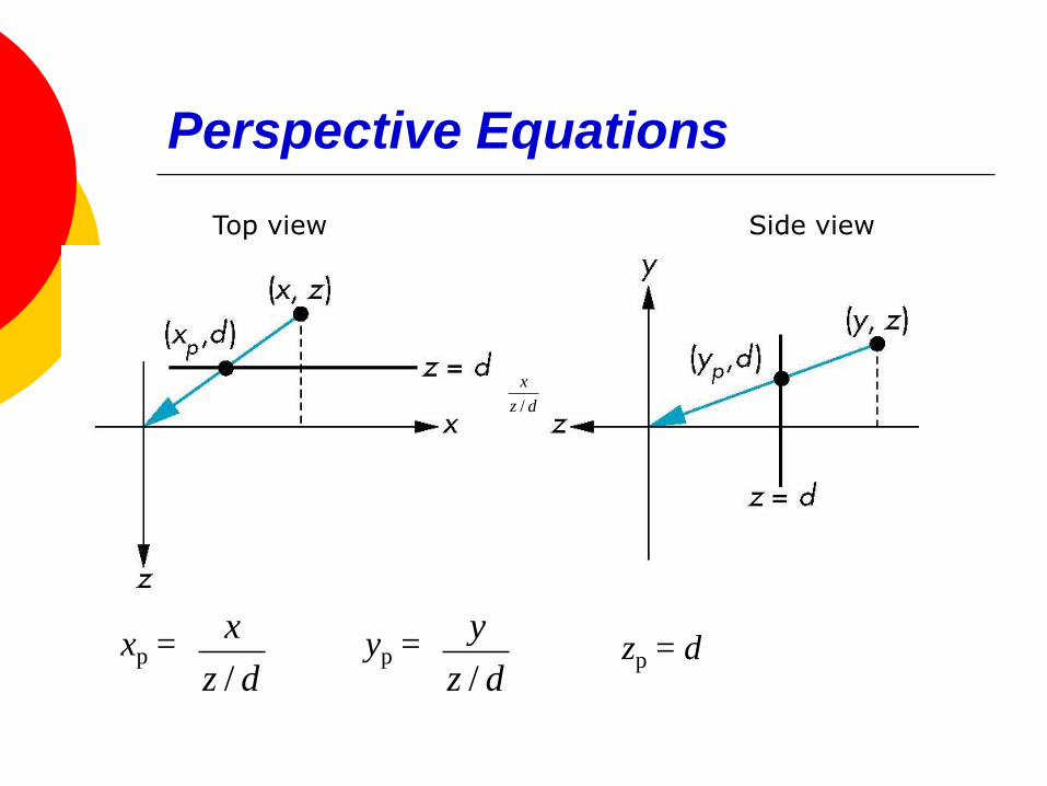
Perspective Equations

xp =

dz

x

/

dz

x

/yp =

dz

y

/zp = d

Top view Side view

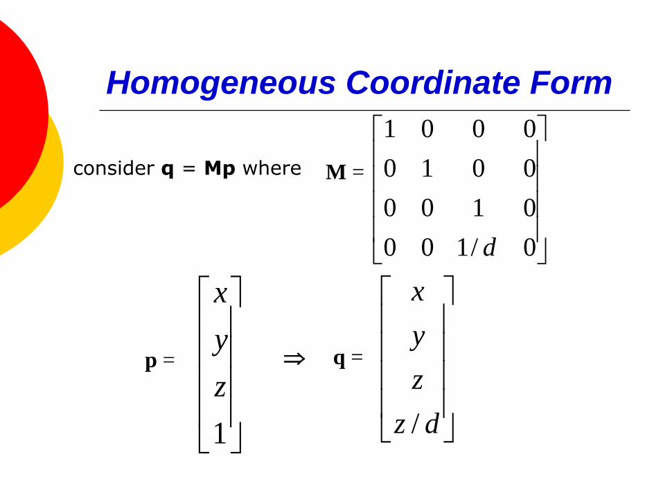
Homogeneous Coordinate Form

M =

0/100

0100

0010

0001

d

consider q = Mp where

1

z

y

x

dz

z

y

x

/

p = q =

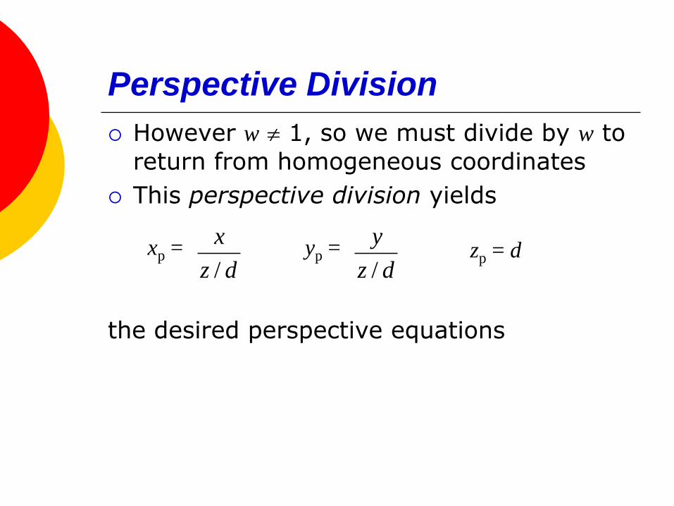
Perspective Division

However w 1, so we must divide by w to

return from homogeneous coordinates

This perspective division yields

the desired perspective equations

xp =dz

x

/yp =

dz

y

/zp = d

Computer Viewing

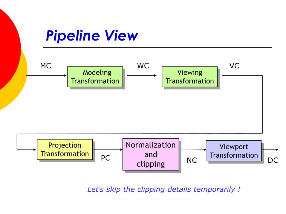
Pipeline View

Modeling

Transformation

Viewing

Transformation

Projection

Transformation

Normalization

and

clipping

Viewport

Transformation

MC WC VC

PC NC DC

Let’s skip the clipping details temporarily !

Computer Viewing

Three aspects of the viewing process implemented in the pipeline:

Positioning the camera

Setting the model-view matrix

Selecting a lens

Setting the projection matrix

Clipping

Setting the view volume

The OpenGL Camera

In OpenGL, initially the object and camera frames are the same

Default model-view matrix is an identity

The camera is located at origin and points in the negative z direction

OpenGL also specifies a default view volume that is a cube with sides of length 2 centered at the origin

Default projection matrix is an identity

Moving the Camera Frame

If we want to visualize object with both positive and negative z values we can either

Move the camera in the positive z direction

Translate the camera frame

Move the objects in the negative z direction

Translate the world frame

Both of these views are equivalent and are determined by the model-view matrix Want a translation (glTranslatef(0.0,0.0,-d);)

d > 0

Moving Camera back from Origin

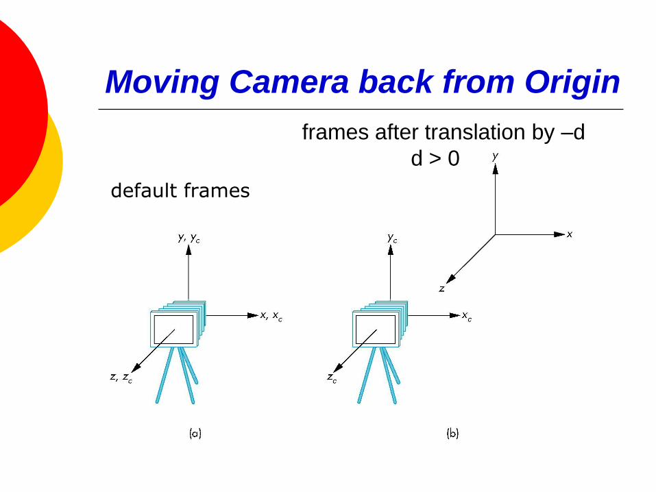
default frames

frames after translation by –d

d > 0

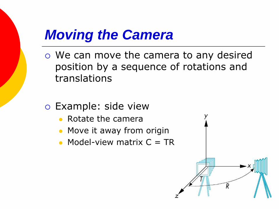
Moving the Camera

We can move the camera to any desired position by a sequence of rotations and translations

Example: side view

Rotate the camera

Move it away from origin

Model-view matrix C = TR

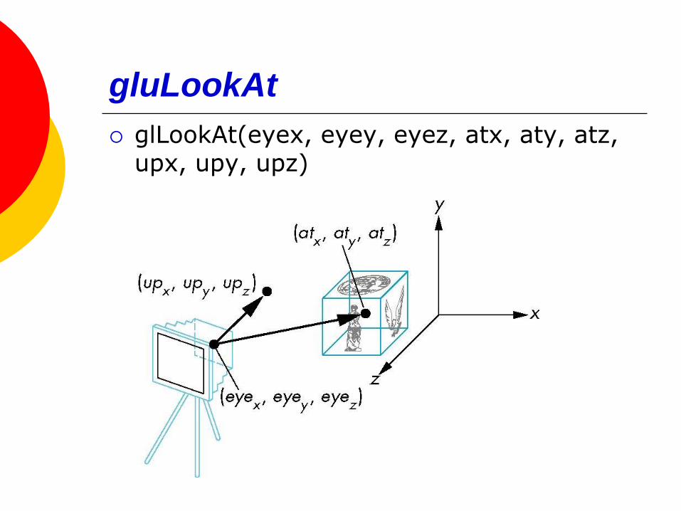
gluLookAt

glLookAt(eyex, eyey, eyez, atx, aty, atz, upx, upy, upz)

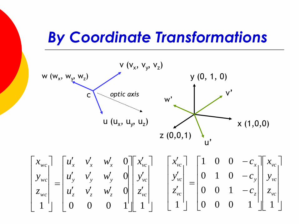
By Coordinate Transformations

11000

0

0

0

1

vc

vc

vc

zzz

yyy

xxx

wc

wc

wc

z

y

x

wvu

wvu

wvu

z

y

x

x (1,0,0)

y (0, 1, 0)

z (0,0,1)u’

v’w’

u (ux, uy, uz)

optic axis

v (vx, vy, vz)

w (wx, wy, wz)

c

11000

100

010

001

1

vc

vc

vc

z

y

x

vc

vc

vc

z

y

x

c

c

c

z

y

x

Taking Clipping into Account

After the view transformation, a simple

projection and viewport transformation can

generate screen coordinate.

However, projecting all vertices are usually

unnecessary.

Clipping with 3D volume.

Associating projection with clipping and

normalization.Why do we use normalization ?

Orthogonal Viewing Volume

Orthogonal Normalization

glOrtho(left,right,bottom,top,near,far)

normalization find transformation to convert

specified clipping volume to default

(xwmin, ywmin, znear)

(xwmax, ywmax, zfar)

(-1, -1, -1)

(1, 1, 1)

xview

Yview

Zview

xnorm

Ynorm

Znorm

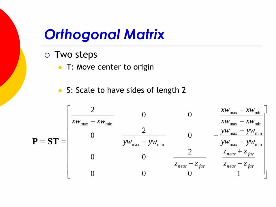
Orthogonal Matrix

Two steps

T: Move center to origin

S: Scale to have sides of length 2

1000

200

02

0

002

minmax

minmax

minmax

minmax

minmax

minmax

farnear

farnear

farnear zz

zz

zz

ywyw

ywyw

ywyw

xwxw

xwxw

xwxw

P = ST =

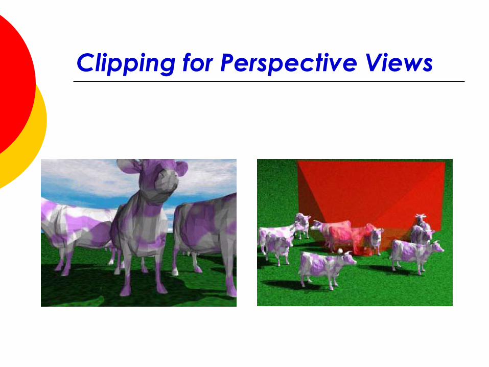
Clipping for Perspective Views

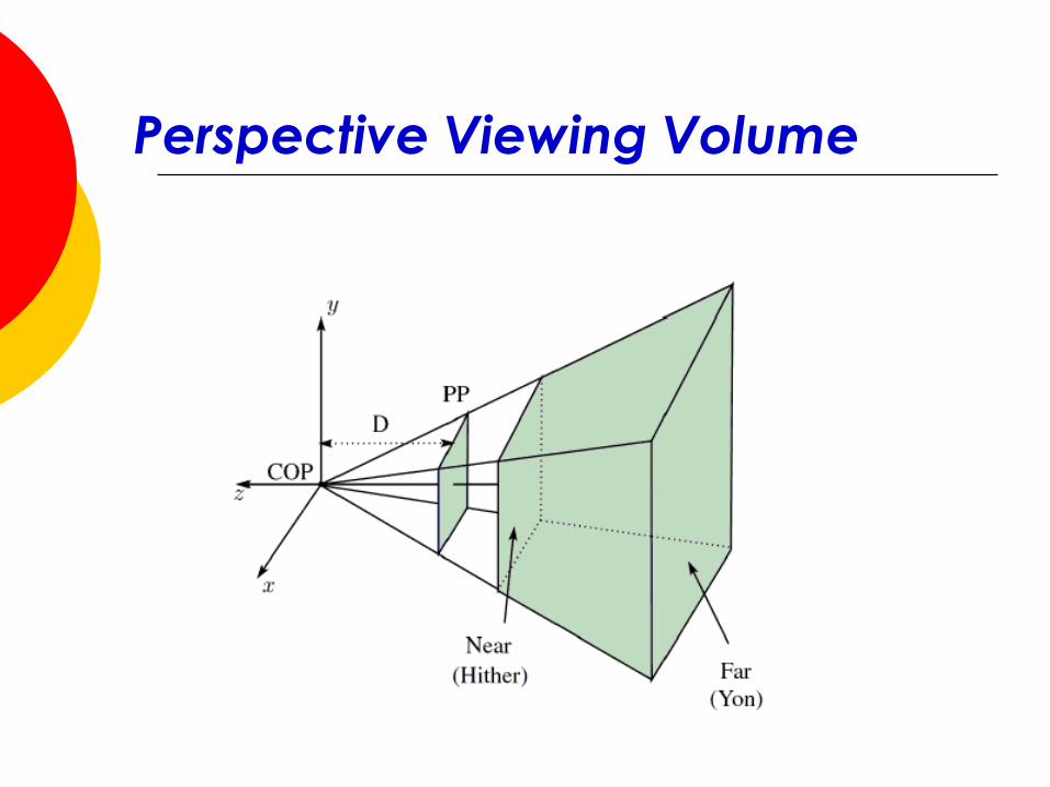
Perspective Viewing Volume

Normalization

Rather than derive a different projection matrix

for each type of projection, we can convert all

projections to orthogonal projections with the

default view volume

This strategy allows us to use standard

transformations in the pipeline and makes for

efficient clipping

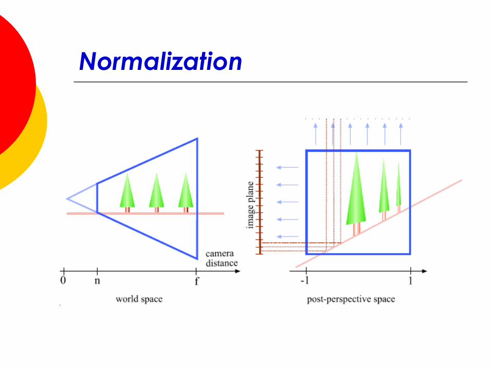
Normalization

Perspective-Projection Trans.

zz

zzy

zz

zzyy

zz

zzx

zz

zzxx

prp

vp

prp

prp

vpprp

p

prp

vp

prp

prp

vpprp

p

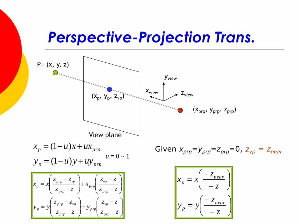
yview

zviewxview

(xprp, yprp, zprp)

P= (x, y, z)

(xp, yp, zvp)

View plane

prpp

prpp

uyyuy

uxxux

)1(

)1(u = 0 ~ 1

Given xprp=yprp=zprp=0, zvp = znear

z

zyy

z

zxx

nearp

nearp

Perspective-Projection Trans.

z

ts

z

tzsz

z

zyy

z

zxx

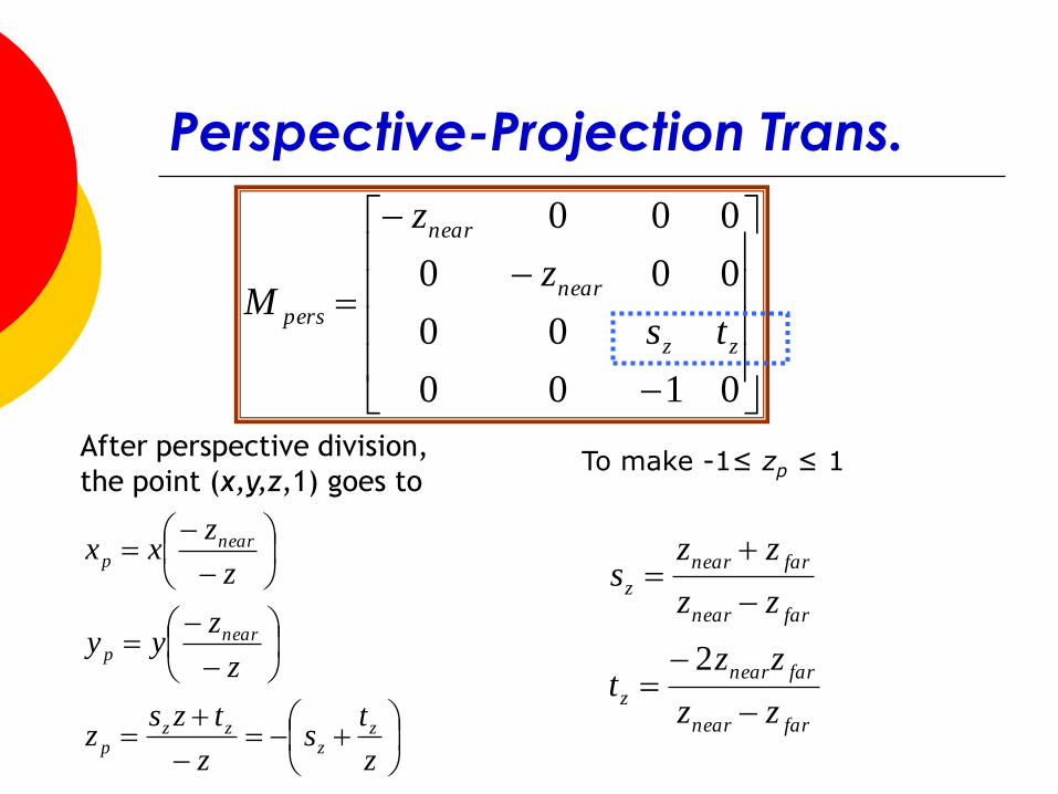
zz

zzp

nearp

nearp

0100

00

000

000

zz

near

near

persts

z

z

M

After perspective division,

the point (x,y,z,1) goes toTo make -1≤ zp ≤ 1

farnear

farnear

z

farnear

farnear

z

zz

zzt

zz

zzs

2

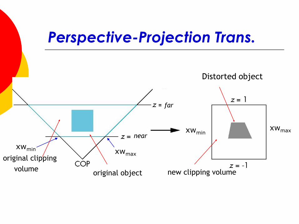
Perspective-Projection Trans.

original object

xwminxwmax

far

near

original clipping

volume new clipping volume

xwmax

xwmin

Distorted object

0100

200

000

000

farnear

farnear

farnear

farnear

near

near

pers

zz

zz

zz

zz

z

z

M

Further Normalization

0100

200

002

0

0002

minmax

minmax

farnear

farnear

farnear

farnear

near

near

normpers

zz

zz

zz

zz

ywywz

xwxwz

M

original object

-1 1

far

near

Notes

Normalization let us clip against a simple cube

regardless of type of projection

Delay final “projection” until end

Important for hidden-surface removal to retain

depth information as long as possible

Normalization and Hidden-

Surface Removal if z1 > z2 in the original clipping volume then the for the

transformed points z1’ < z2’

Hidden surface removal works if we first apply the normalization transformation

However, the formula z’’ = -(sz+tz/z) implies that the distances are distorted by the normalization which can cause numerical problems especially if the near distance is small

Why do we do it this way?

Normalization allows for a single pipeline for both perspective and orthogonal viewing

We stay in four dimensional homogeneous coordinates as long as possible to retain three-dimensional information needed for hidden-surface removal and shading

Clipping is now “easiler”.

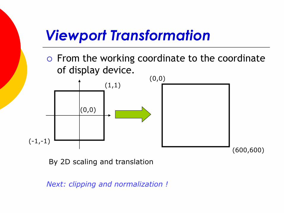
Viewport Transformation

From the working coordinate to the coordinate

of display device.

(1,1)

(-1,-1)

(0,0)

(0,0)

(600,600)

By 2D scaling and translation

Next: clipping and normalization !

APPENDIX

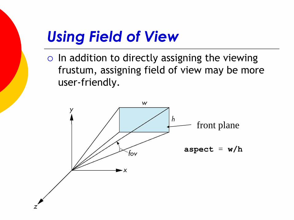
Using Field of View

In addition to directly assigning the viewing

frustum, assigning field of view may be more

user-friendly.

aspect = w/h

front plane

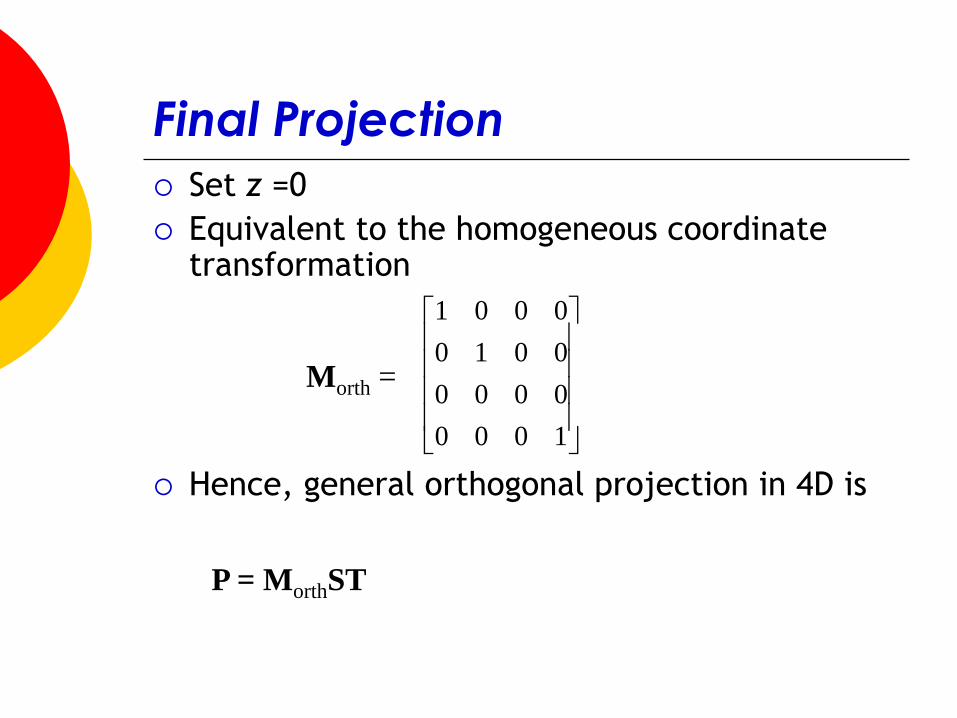
Final Projection

Set z =0

Equivalent to the homogeneous coordinate transformation

Hence, general orthogonal projection in 4D is

1000

0000

0010

0001

Morth =

P = MorthST

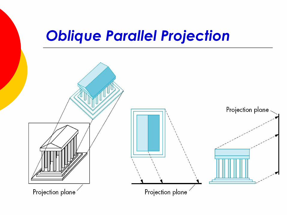
Oblique Parallel Projection

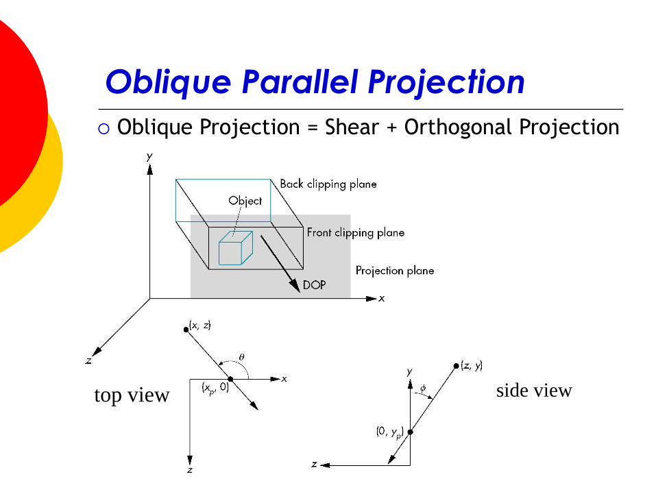
Oblique Parallel Projection

top view side view

Oblique Projection = Shear + Orthogonal Projection

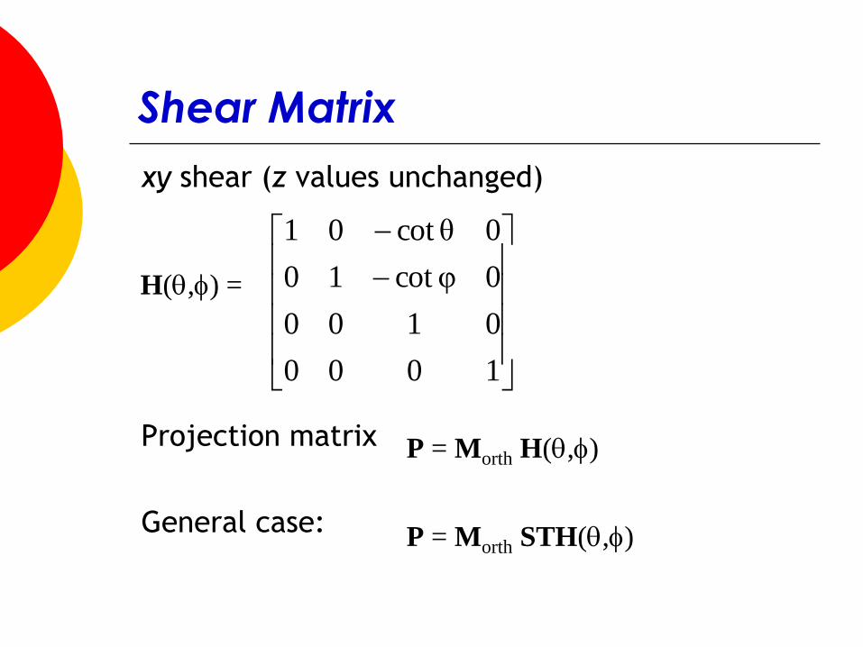
Shear Matrix

xy shear (z values unchanged)

Projection matrix

General case:

1000

0100

0φcot10

0θcot01

H(q,f) =

P = Morth H(q,f)

P = Morth STH(q,f)

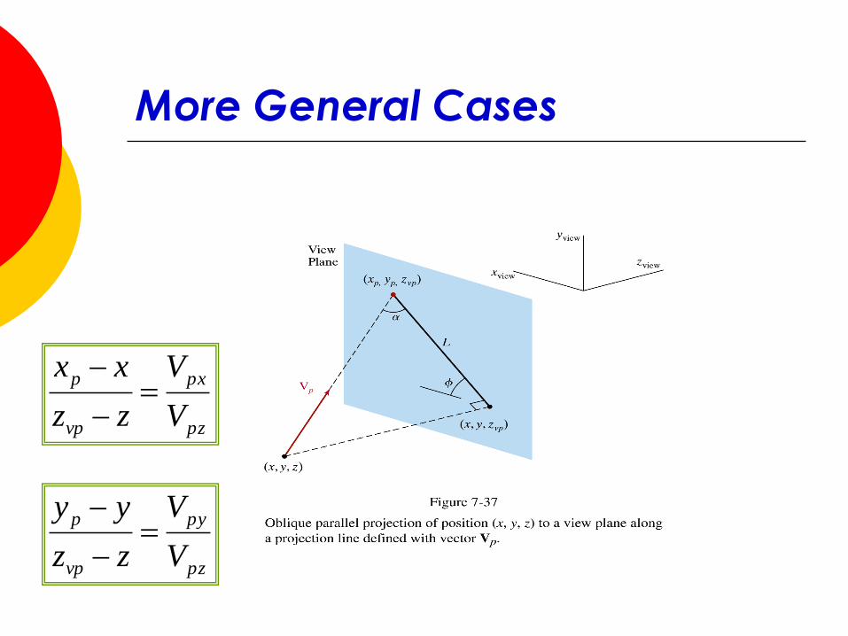
More General Cases

pz

px

vp

p

V

V

zz

xx

pz

py

vp

p

V

V

zz

yy

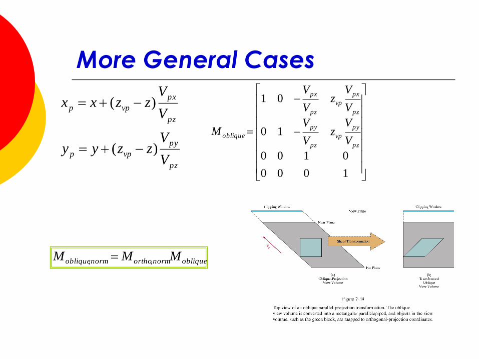
More General Cases

pz

py

vpp

pz

px

vpp

V

Vzzyy

V

Vzzxx

)(

)(

1000

0100

10

01

pz

py

vp

pz

py

pz

px

vp

pz

px

obliqueV

Vz

V

V

V

Vz

V

V

M

obliquenormorthonormoblique MMM ,,

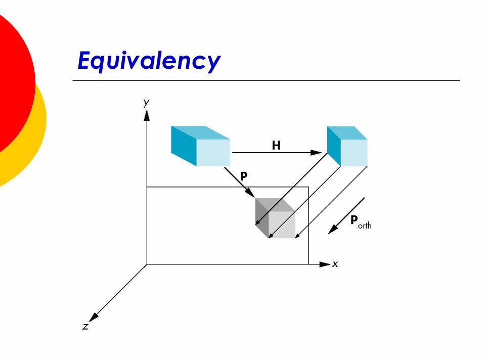
Equivalency

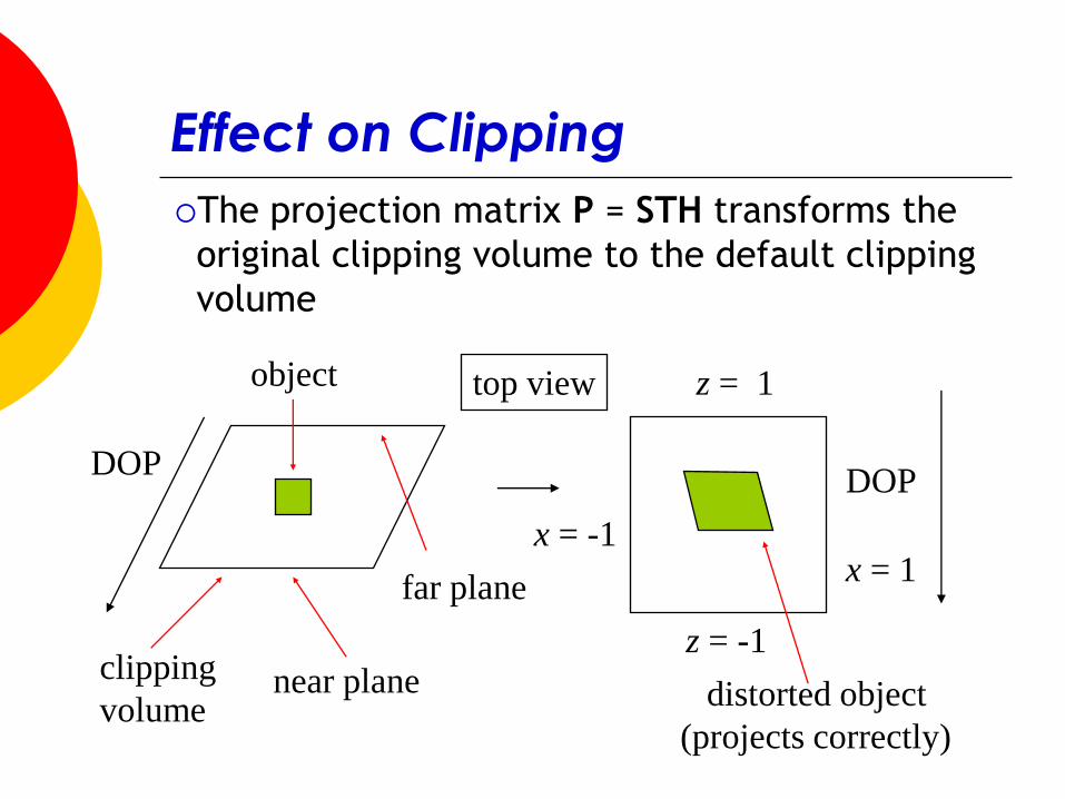
Effect on Clipping

The projection matrix P = STH transforms the

original clipping volume to the default clipping

volume

top view

DOPDOP

near plane

far plane

object

clipping

volume

z = -1

z = 1

x = -1x = 1

distorted object

(projects correctly)