Embed Size (px)
Citation preview

1 Dr. Peter AvitabileModal Analysis & Controls Laboratory22.451 Dynamic Systems – Intro to Controls
Introduction to Control Systems
Peter AvitabileMechanical Engineering DepartmentUniversity of Massachusetts Lowell
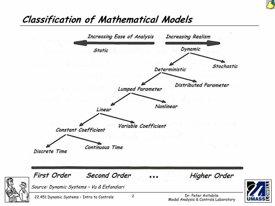
Stochastic
Dynamic
Deterministic
Distributed ParameterLumped Parameter
NonlinearLinear
Variable CoefficientConstant Coefficient
Continuous TimeDiscrete Time
Static
Increasing Ease of Analysis Increasing Realism
First Order Second Order Higher Order
CLASSIFICATION OF MATHEMATICAL MODELS
2 Dr. Peter AvitabileModal Analysis & Controls Laboratory22.451 Dynamic Systems – Intro to Controls
Classification of Mathematical Models
Source: Dynamic Systems – Vu & Esfandiari

3 Dr. Peter AvitabileModal Analysis & Controls Laboratory22.451 Dynamic Systems – Intro to Controls
Introduction to Control SystemsDefinitions
Closed Loop System – there always exists some ‘feedback’ of one or more variables that influence the input excitation.
Disturbance Inputs – signal that exists but no control is possible.
Negative/Positive Feedback – signals that are added to or subtracted from an input signal.
Open Loop System – no feedback signals are available to the control system.Plant – device, system or component that is described by some transfer relation.Essential Components of a Control System – Plant, Sensor, Actuator, Controller
4 Dr. Peter AvitabileModal Analysis & Controls Laboratory22.451 Dynamic Systems – Intro to Controls
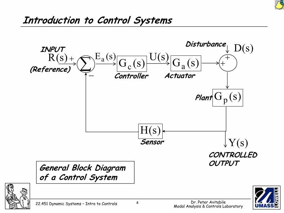
Introduction to Control Systems
(Reference))s(R + )s(Gc
)s(H
−∑
)s(Ea )s(Ga)s(U +
+
)s(DDisturbance
Sensor
Controller Actuator
Plant )s(Gp
INPUT
)s(YCONTROLLED OUTPUTGeneral Block Diagram
of a Control System
5 Dr. Peter AvitabileModal Analysis & Controls Laboratory22.451 Dynamic Systems – Intro to Controls
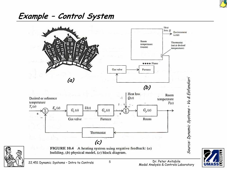
Example – Control System
Sour
ce: D
ynam
ic S
yste
ms
–Vu
& Es
fand
iari(a)
(b)
(c)

6 Dr. Peter AvitabileModal Analysis & Controls Laboratory22.451 Dynamic Systems – Intro to Controls
Introduction to Control Systems
Knowledge of the system Poles and Zeros is important information in the design and analysis of dynamic systems, vibrations, and controls.Assume a system transfer function such as:
poleszeros
rdenominatonumerator
)s(D)s(N.F.T ⇒==
Poles and Zeros
The numerator polynomial can be factored to identify the system transfer function ZEROS. The denominator polynomial can also be factored to identify the system transfer function POLES.
( )( )2s1s5.0s
2s3s5.0s.F.T 2 ++
+=
+++
=
Xby denotedOby denoted
2,1POLES5.0ZERO→→
−−→−→
Im
Re
POLEZERO
X XO2- 1-

7 Dr. Peter AvitabileModal Analysis & Controls Laboratory22.451 Dynamic Systems – Intro to Controls
Time Constant – First Order System
)t(fvv =+τ&
Differential Equation
01s =+τ
Characteristic Equation
Pole
τ−=
1s
Im
ReXτ1
−

8 Dr. Peter AvitabileModal Analysis & Controls Laboratory22.451 Dynamic Systems – Intro to Controls
Time Constant – First Order System
)t(fxcxm =+ &&&
Consider the mechanical system shown
then
OR
cm
=τ
m fcx,x &
)t(fcvvm =+&
ORc
)t(fvvcm
=+
&c
)t(fvv =+τ&
The time constant is

9 Dr. Peter AvitabileModal Analysis & Controls Laboratory22.451 Dynamic Systems – Intro to Controls
First Order System – RC Circuit
( )( )( )20s7s1s140)s(h
+++=
Consider the function of an RC circuit
Slowest Pole
Written in POLE-ZERO form, the block diagram is
( ) ( ) ( )20s20
7s7
1s1
FX
+++=
F1s
1+ 7s
7+ 20s
20+
Quicker Pole
Fastest Pole
X

10 Dr. Peter AvitabileModal Analysis & Controls Laboratory22.451 Dynamic Systems – Intro to Controls
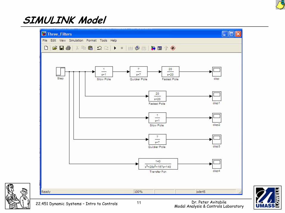
First Order System – RC CircuitA SIMULINK Model can be used to quickly see the response of each pole.
STEP
1s1+
7s7+
20s20+
SUMX( )( )( )20s7s1s
140+++
1X
7X
20X
The pole ‘closest’ to the jω axis dominates the time response of the system.
11 Dr. Peter AvitabileModal Analysis & Controls Laboratory22.451 Dynamic Systems – Intro to Controls
SIMULINK Model

12 Dr. Peter AvitabileModal Analysis & Controls Laboratory22.451 Dynamic Systems – Intro to Controls
Time Constant – Second Order System
)t(fxx2x 2nn =ω+ζω+ &&&
Differential Equation
Pole - Overdamped
1s 2nn2,1 −ζω±ζω−=
0s2s 2nn
2 =ω+ζω+Characteristic Equation
Pole – Critically damped
n2,1s ω−= (repeated)Pole – Underdamped
2nn2,1 1js ζ−ω±ζω−=
djω±σ−=Pole – Undamped
n2,1 js ω±=
ImReX
ImRe
ImRe
ImRe
X
XX
X
XX

13 Dr. Peter AvitabileModal Analysis & Controls Laboratory22.451 Dynamic Systems – Intro to Controls
Time Constant – Second Order System
)t(fkxxcxm =++ &&&
Consider the mechanical system
with
OR
which is written in standard form as
m)t(fx
mkx
mcx =++ &&&
mk
n =ω
km2c
m2c
cc
nc=
ω==ζ
m)t(fxx2x 2
nn =ω+ζω+ &&&

14 Dr. Peter AvitabileModal Analysis & Controls Laboratory22.451 Dynamic Systems – Intro to Controls
Transient Response Specification TermsMaximum Percent Overshoot – Mp%
The maximum overshoot is the maximum amplitude expressed as a percentage of the steady state value.
Settling Time - ts
21p eM ζ−
πζ−
=
The time required for the response to reach a small percentage of steady state value.
σ=
ζω=τ=≈
444'ttn
%2s%2s
σ=
ζω=τ=≈
333'ttn
%5s%5s

15 Dr. Peter AvitabileModal Analysis & Controls Laboratory22.451 Dynamic Systems – Intro to Controls
Transient Response Specification Terms
Rise Time – tr
The time for an underdamped2nd order system to rise from 0 to 100% of the final steady state value.
ζζ−
ω−= −
21
nr
1tan1t
Peak Time – tp
The time required to reach maximum overshoot is called peak time. d
ptωπ
=

16 Dr. Peter AvitabileModal Analysis & Controls Laboratory22.451 Dynamic Systems – Intro to Controls
Transient Response Specification Terms

17 Dr. Peter AvitabileModal Analysis & Controls Laboratory22.451 Dynamic Systems – Intro to Controls
Transfer Functions Building Block MethodologyAll transfer functions can be broken down into pieces (called building blocks) for evaluation and assessment.
( )( )( )500s101s2ss
90s750)s(H 2 +++
+=
These can be categorized as•constant•first order pole (or zero) at origin•first order pole (or zero) not at origin•second order pole (or zero) with damping ratio less than 1.0
For Example:Constant 1st Order Zero
(not at origin)
1st Order Pole (not at origin)2nd Order Pole
Damping < 1.01st Order Pole (at origin)

18 Dr. Peter AvitabileModal Analysis & Controls Laboratory22.451 Dynamic Systems – Intro to Controls
Transfer Functions Building Block MethodologyFirst Order Pole At Origin
s1)s(G =
ω=ω
j1)j(G
First Order Pole
Second Order Pole
dB Mag
log f
20 dB/octave
dB Mag
log f
20 dB/octave
dB Mag
log f
40 dB/octave
aj1)j(G+ω
=ω
as1)s(G+
=
2nn
2
2n
s2s)s(G
ω+ζω+
ω=
( ) ( ) 2nn
2
2n
j2j)j(G
ω+ωζω+ω
ω=ω

19 Dr. Peter AvitabileModal Analysis & Controls Laboratory22.451 Dynamic Systems – Intro to Controls
Transfer Functions Building Block MethodologyFirst Order Zero At Origin
s)s(G =ω=ω j)j(G
First Order Zero
Second Order Zero
dB Mag
log f
20 dB/octave
dB Mag
log f
20 dB/octave
dB Mag
log f
40 dB/octave
aaj)j(G +ω
=ω
aas)s(G +
=
2n
2nn
2 s2s)s(Gω
ω+ζω+=
( ) ( )2
n
2nn
2 j2j)j(Gω
ω+ωζω+ω=ω

20 Dr. Peter AvitabileModal Analysis & Controls Laboratory22.451 Dynamic Systems – Intro to Controls
Controller Types•On/Off•Differential On/Off•Proportional Control (P control)•Derivative Control (D control)•Integral Control (I control)•PD Control •PI Control•PID Control
Others (Advanced Methods)•Lead Network Control•Lag Network Control•Lead-Lag Network Control•Feed Forward Control

21 Dr. Peter AvitabileModal Analysis & Controls Laboratory22.451 Dynamic Systems – Intro to Controls
Controller TypesOn/Off
)t(e 01
01M
2MOR
Differential
Differential
Example: Home heating system
22 Dr. Peter AvitabileModal Analysis & Controls Laboratory22.451 Dynamic Systems – Intro to Controls
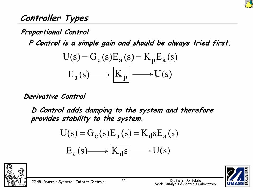
Controller Types
P Control is a simple gain and should be always tried first.
pK)s(Ea )s(U
)s(EK)s(E)s(G)s(U apac ==
sKd)s(Ea )s(U
Proportional Control
D Control adds damping to the system and therefore provides stability to the system.
Derivative Control
)s(sEK)s(E)s(G)s(U adac ==

23 Dr. Peter AvitabileModal Analysis & Controls Laboratory22.451 Dynamic Systems – Intro to Controls
Controller Types
I Control reduces steady state error but can increase instability.
sK I)s(E a )s(U
)s(Es
K)s(E)s(G)s(U aI
ac ==
Integral Control

24 Dr. Peter AvitabileModal Analysis & Controls Laboratory22.451 Dynamic Systems – Intro to Controls
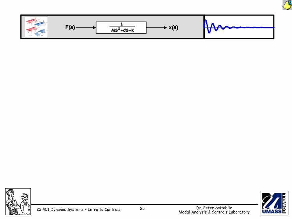
Controller Types
sKs
KK dI
p ++)s(E a )s(U
Desired Value of Control Variable
PID Control
)s(EsKs
KK)s(E)s(G)s(U adI
pac
++==
+
−∑ sK
sKK d
Ip ++
Plant
)s(M
25 Dr. Peter AvitabileModal Analysis & Controls Laboratory22.451 Dynamic Systems – Intro to Controls