Introduction to Digital Signal Processing

(Discrete-time Signal Processing)

Prof. Chu-Song Chen Research Center for Info. Tech. Innovation,

Academia Sinica, Taiwan Dept. CSIE & GINM

National Taiwan University

Fall 2013

• In our technical society we often measure a continuously varying (analog) quantity. eg. Blood pressure, earthquake displacement, population of a city, waves falling on a beach, and the probability of death.

• All these measurement varying with time; we regard them as functions of time: x(t) in mathematical notation.

Signals

→ flow of information

→ measured quantity that varies with time (or position)

→ electrical signal received from a transducer

(microphone, thermometer, accelerometer, antenna, etc.)

→ electrical signal that controls a process

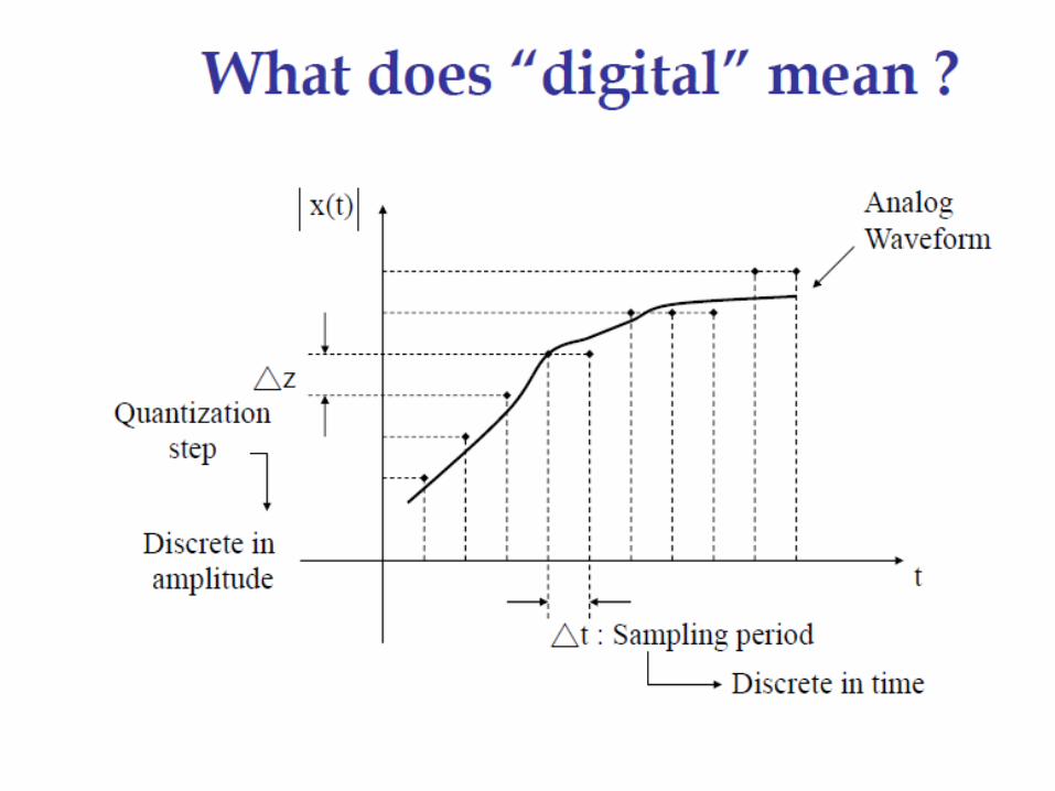
• For technical reasons, instead of the signal x(t), we usually record equally spaced samples xn of the function x(t). (discrete-time) – The sampling theorem gives the conditions on the signal

that justify this sampling process.

– i.e., discrete-time signal is a sequence of numbers

• Moreover, when the samples are taken they are not recorded with infinite precision but are rounded off (sometimes chopped off) to comparatively few digits.

• This procedure is often called quantizing the samples. (digital)

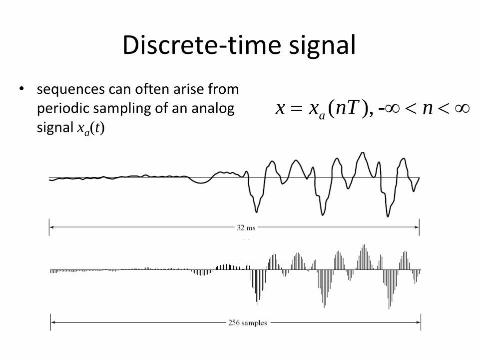
Discrete-time signal

• sequences can often arise from periodic sampling of an analog signal xa(t)

n-nTxx a ),(

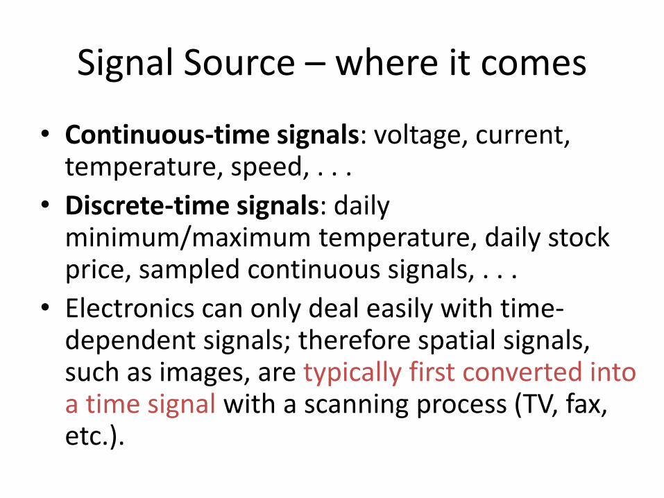
Signal Source – where it comes

• Continuous-time signals: voltage, current, temperature, speed, . . .

• Discrete-time signals: daily minimum/maximum temperature, daily stock price, sampled continuous signals, . . .

• Electronics can only deal easily with time-dependent signals; therefore spatial signals, such as images, are typically first converted into a time signal with a scanning process (TV, fax, etc.).

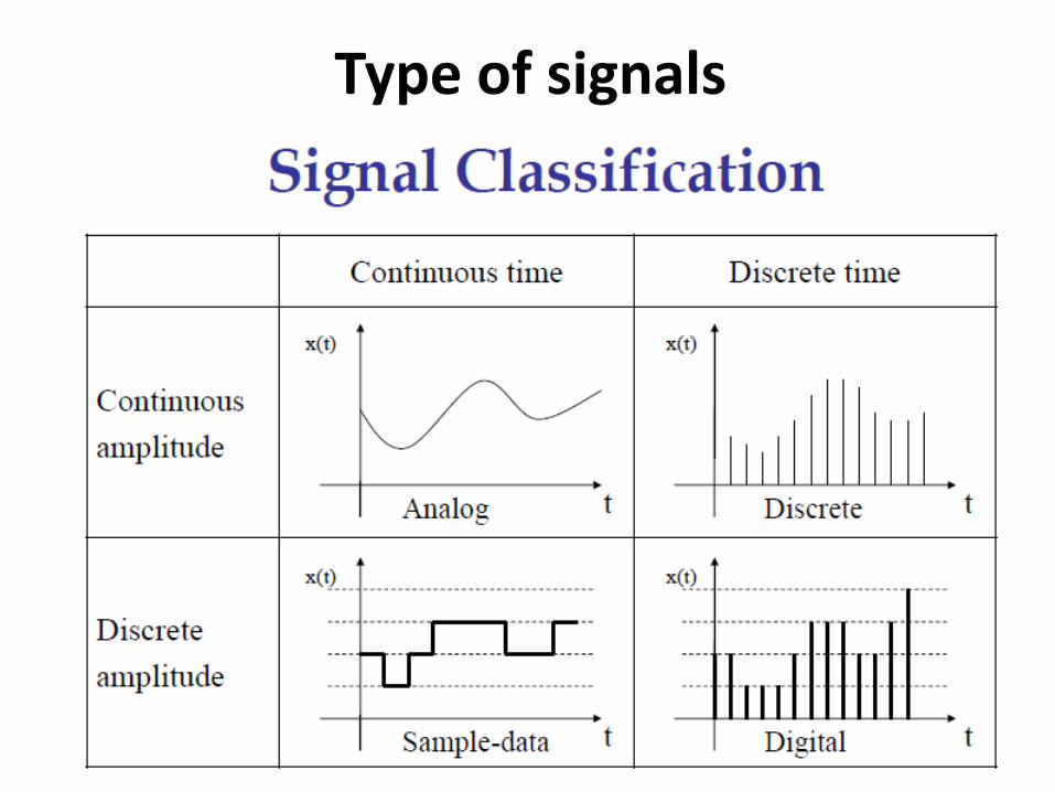
Type of signals

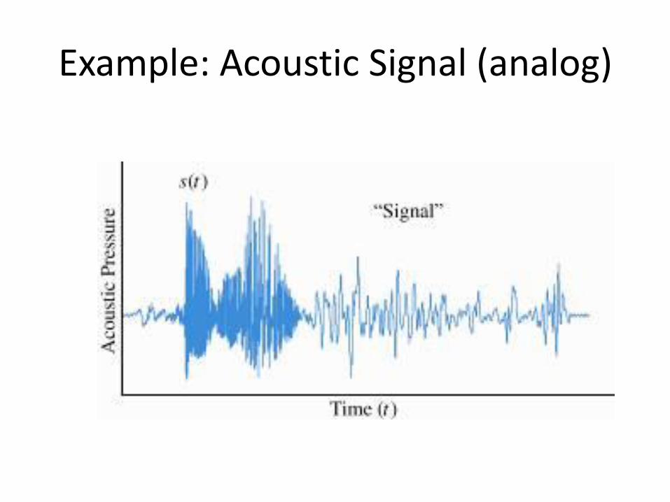
Example: Acoustic Signal (analog)

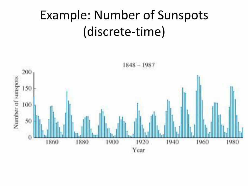
Example: Number of Sunspots (discrete-time)

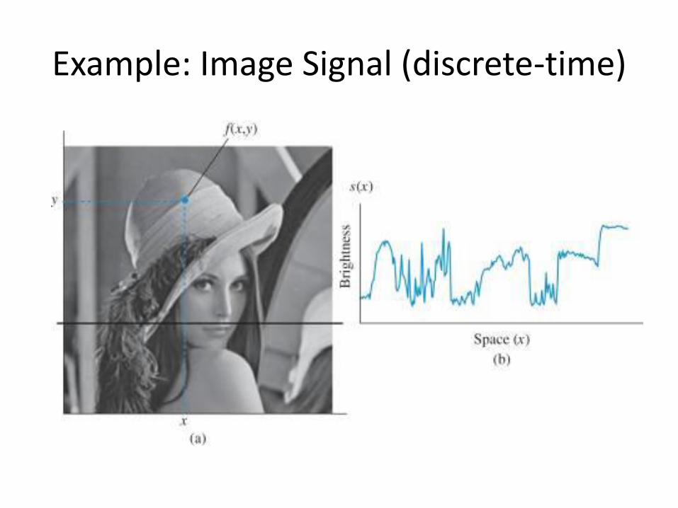
Example: Image Signal (discrete-time)

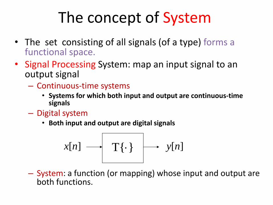
The concept of System

• The set consisting of all signals (of a type) forms a functional space.

• Signal Processing System: map an input signal to an output signal – Continuous-time systems

• Systems for which both input and output are continuous-time signals

– Digital system • Both input and output are digital signals

– System: a function (or mapping) whose input and output are both functions.

x[n] T{} y[n]

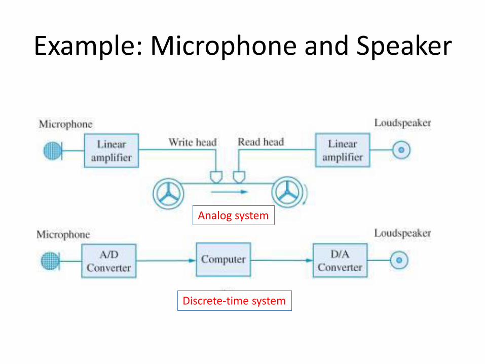
Example: Microphone and Speaker

Analog system

Discrete-time system

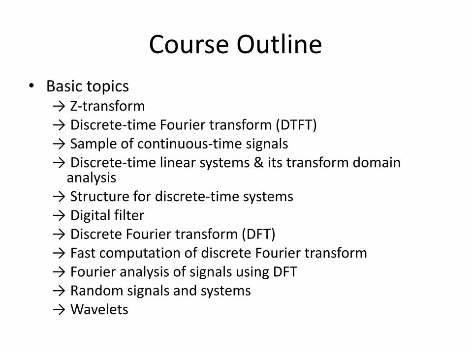
Course Outline

• Basic topics → Z-transform → Discrete-time Fourier transform (DTFT) → Sample of continuous-time signals → Discrete-time linear systems & its transform domain

analysis → Structure for discrete-time systems → Digital filter → Discrete Fourier transform (DFT) → Fast computation of discrete Fourier transform → Fourier analysis of signals using DFT → Random signals and systems → Wavelets

• Reference Textbooks – James H. McClellan, Ronald W. Schafer, and Mark A.

Yoader, Signal Processing First – Alan V. Oppenheim and Ronald W. Schafer, Discrete-

Time Signal Processing, Prentice-Hall. – Boaz Porat, A Course in Digital Signal Processing – Dimitris G. Manolakis and Vinay K. Ingle, Applied Digital

Signal Processing

• Main Journals – IEEE Trans. Signal Processing – IEEE Signal Processing Magazine

• Main Conferences – IEEE International Conference on ASSP (ICASSP)

Course Information

• Teaching assistant: – Yin-Tzu Lin 林映孜

known@cmlab.csie.ntu.edu.tw

• Course webpage: – www.cmlab.csie.ntu.edu.tw/~dsp/dsp2013

• Grades – Homework x several (30%)

– Test x 2~3 (40~45%)

– Term project (25~30%)

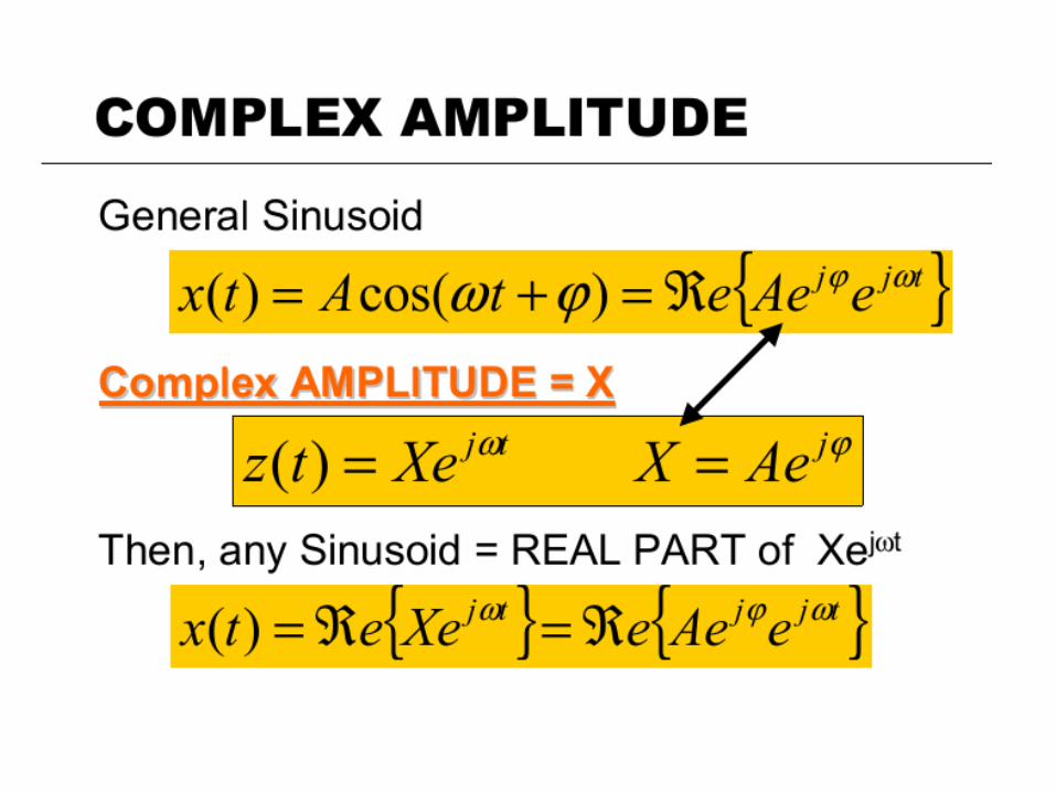
Frequency and Sinusoids

• Signal processing is originated form the processing of frequency.

• Understanding the frequency: better from sinusoidal functions.

– Important to the field of broadcasting, wireless communication, music analysis, etc.

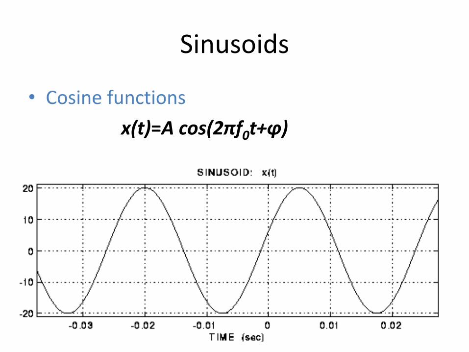
Sinusoids

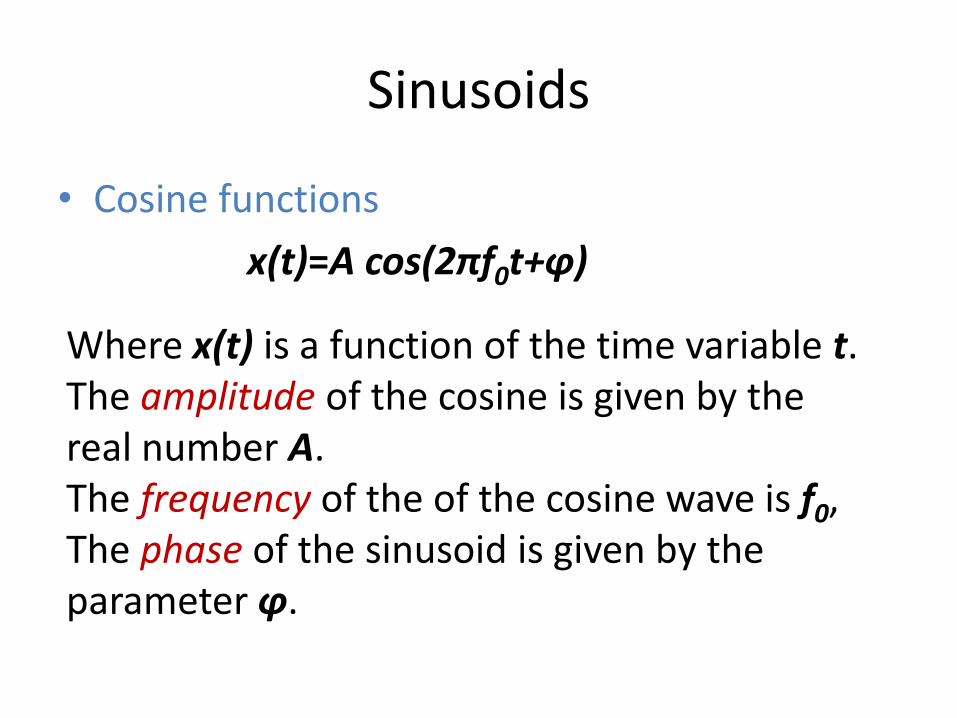
• Cosine functions

x(t)=A cos(2πf0t+φ)

Sinusoids

• Cosine functions

x(t)=A cos(2πf0t+φ)

Where x(t) is a function of the time variable t. The amplitude of the cosine is given by the real number A. The frequency of the of the cosine wave is f0, The phase of the sinusoid is given by the parameter φ.

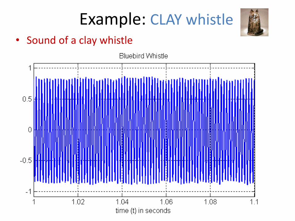
Example: CLAY whistle • Sound of a clay whistle

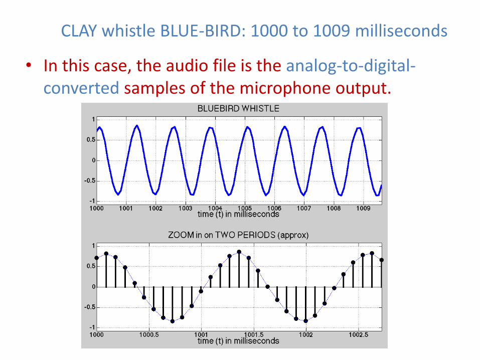
CLAY whistle BLUE-BIRD: 1000 to 1009 milliseconds

• In this case, the audio file is the analog-to-digital-converted samples of the microphone output.

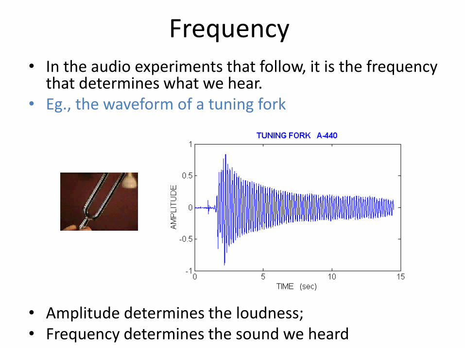
Frequency • In the audio experiments that follow, it is the frequency

that determines what we hear. • Eg., the waveform of a tuning fork

• Amplitude determines the loudness; • Frequency determines the sound we heard

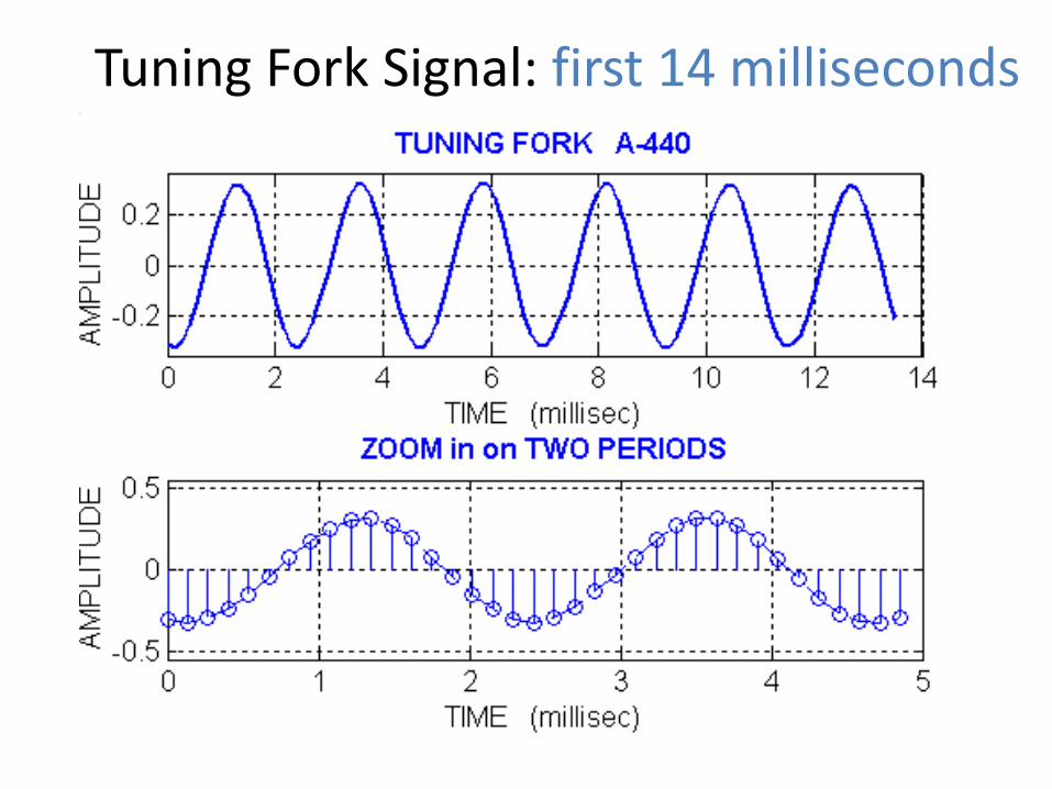
Tuning Fork Signal: first 14 milliseconds

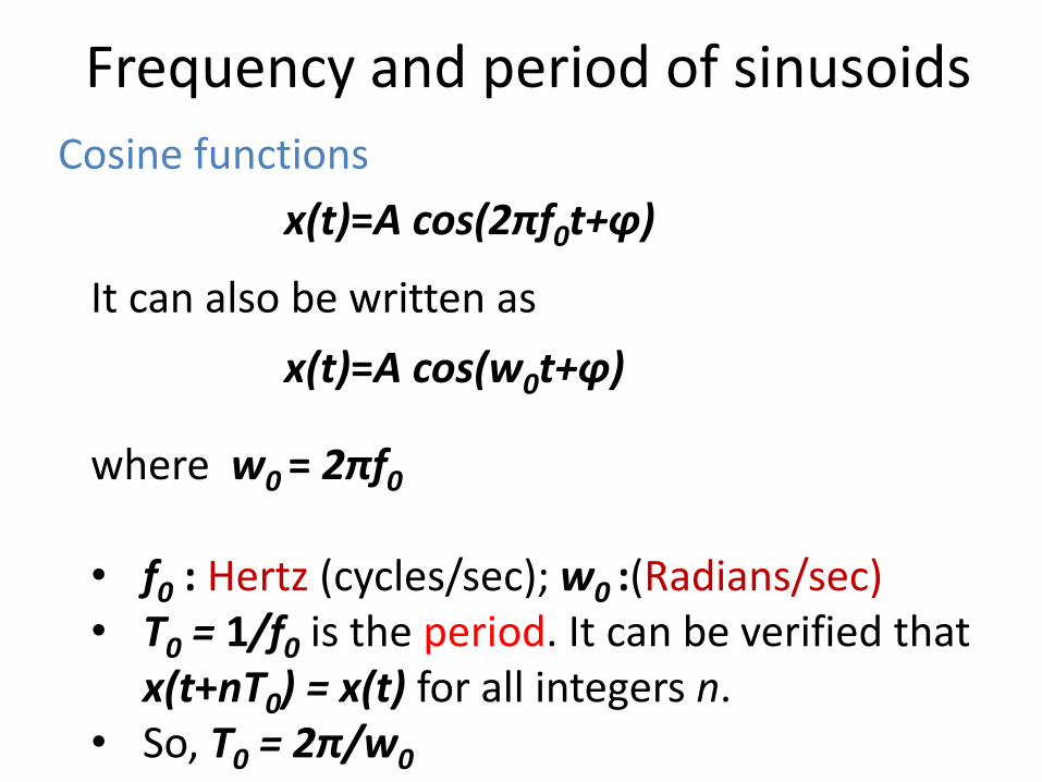
Frequency and period of sinusoids

Cosine functions

x(t)=A cos(2πf0t+φ)

It can also be written as where w0 = 2πf0 • f0 : Hertz (cycles/sec); w0 :(Radians/sec) • T0 = 1/f0 is the period. It can be verified that

x(t+nT0) = x(t) for all integers n. • So, T0 = 2π/w0

x(t)=A cos(w0t+φ)

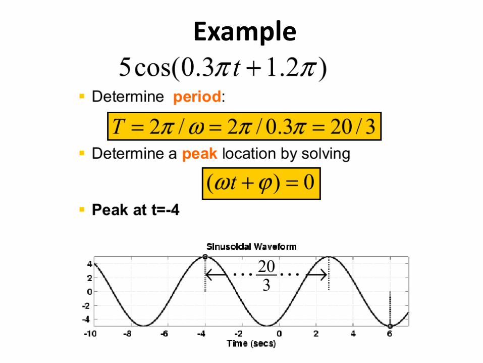
Example

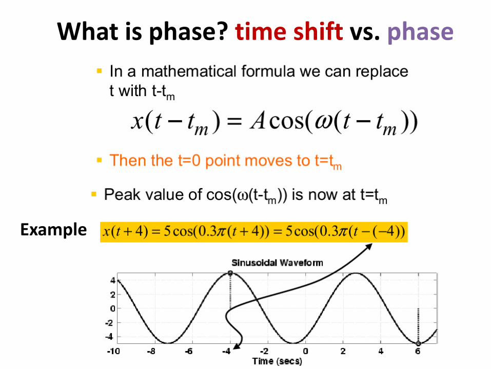
What is phase? time shift vs. phase

Example

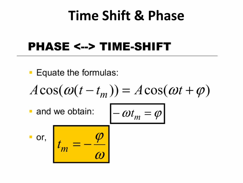
Time Shift & Phase

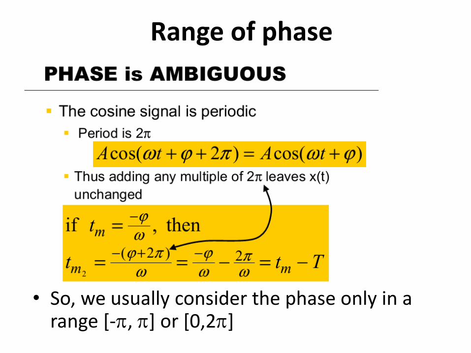
Range of phase

• So, we usually consider the phase only in a range [-, ] or [0,2]

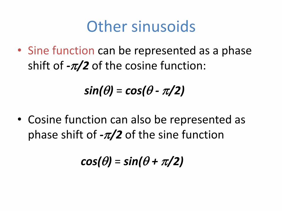
Other sinusoids

• Sine function can be represented as a phase shift of -/2 of the cosine function:

• Cosine function can also be represented as phase shift of -/2 of the sine function

sin() = cos( - /2)

cos() = sin( + /2)

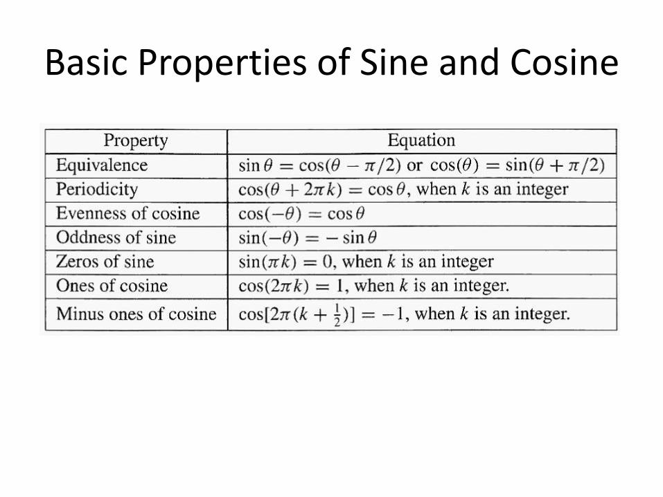
Basic Properties of Sine and Cosine

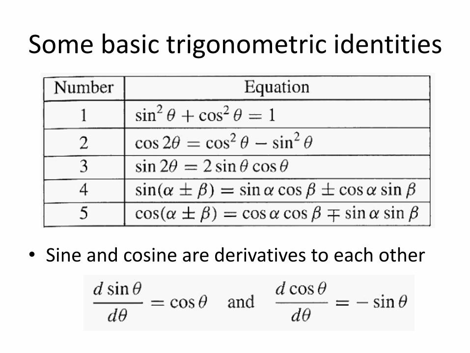
Some basic trigonometric identities

• Sine and cosine are derivatives to each other

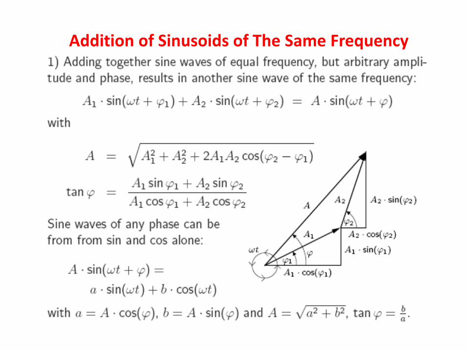
Addition of Sinusoids of The Same Frequency

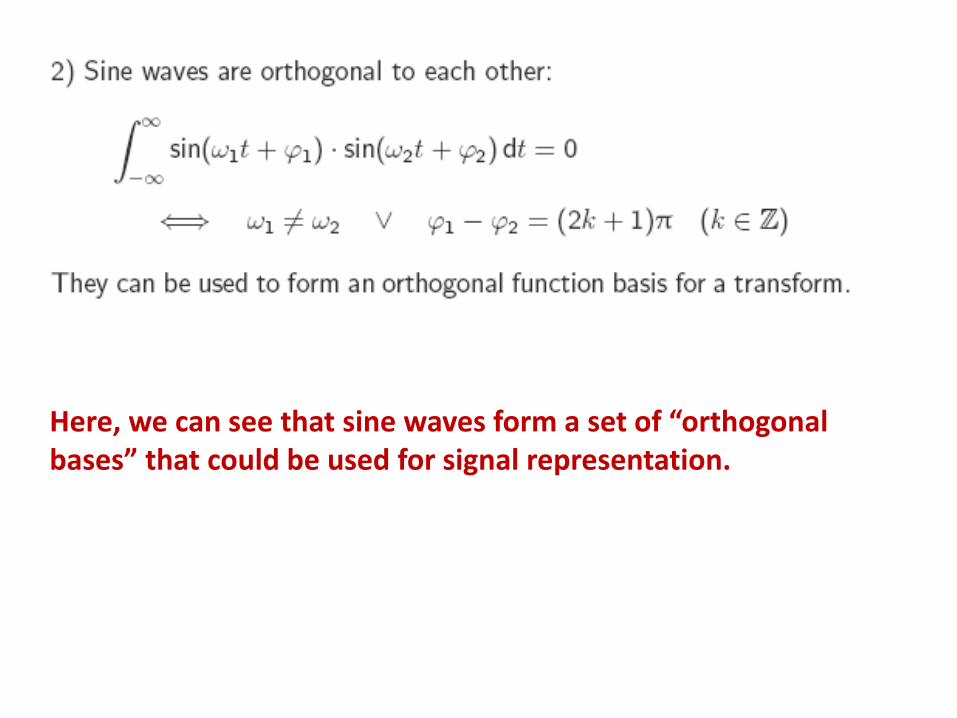
Here, we can see that sine waves form a set of “orthogonal bases” that could be used for signal representation.

Basis Functions for Decompositions

• As mentioned, signal processing is originated form the processing of “frequency.”

• We hope to decompose the signals by extracting its components with respect to different frequencies.

• In other words, we hope to represent a signal as a linear combination of “bases functions.”

• What are the proper basis functions for frequency decomposition? Sine or Cosine?

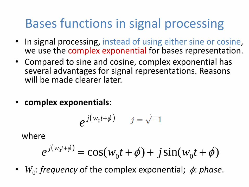
Bases functions in signal processing • In signal processing, instead of using either sine or cosine,

we use the complex exponential for bases representation. • Compared to sine and cosine, complex exponential has

several advantages for signal representations. Reasons will be made clearer later.

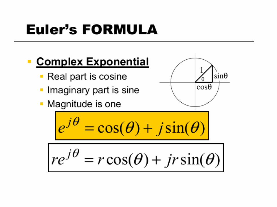
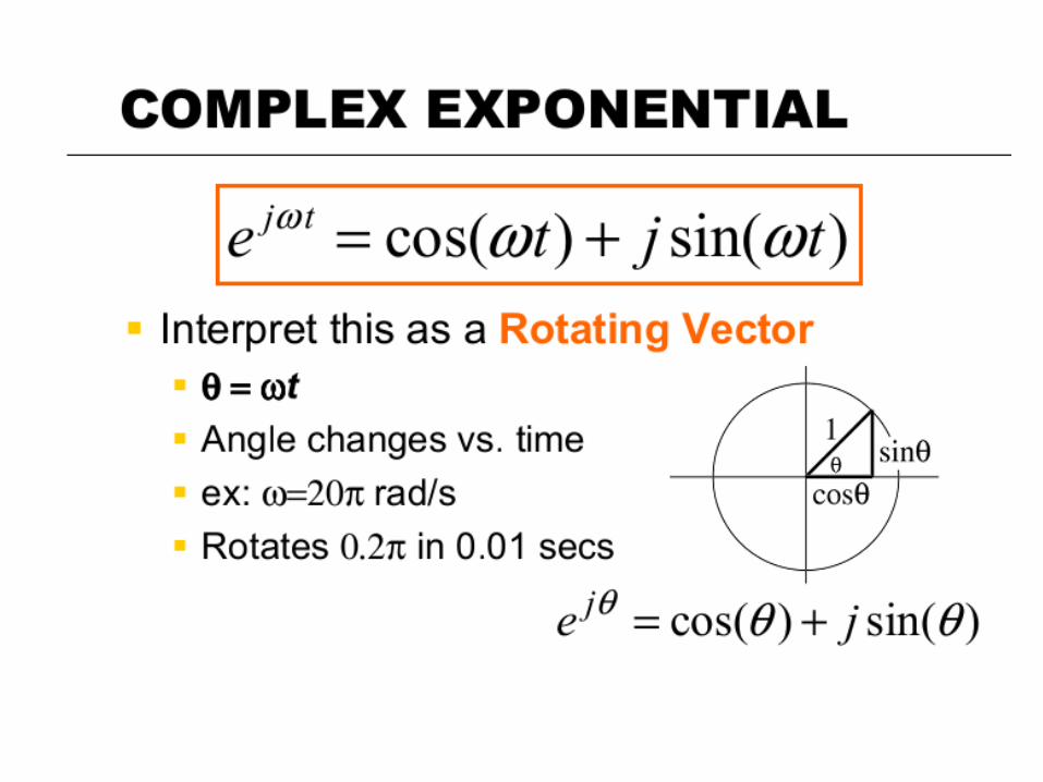
• complex exponentials:

where

• W0: frequency of the complex exponential; : phase.

twje 0

)sin()cos( 00

0

twjtwe

twj

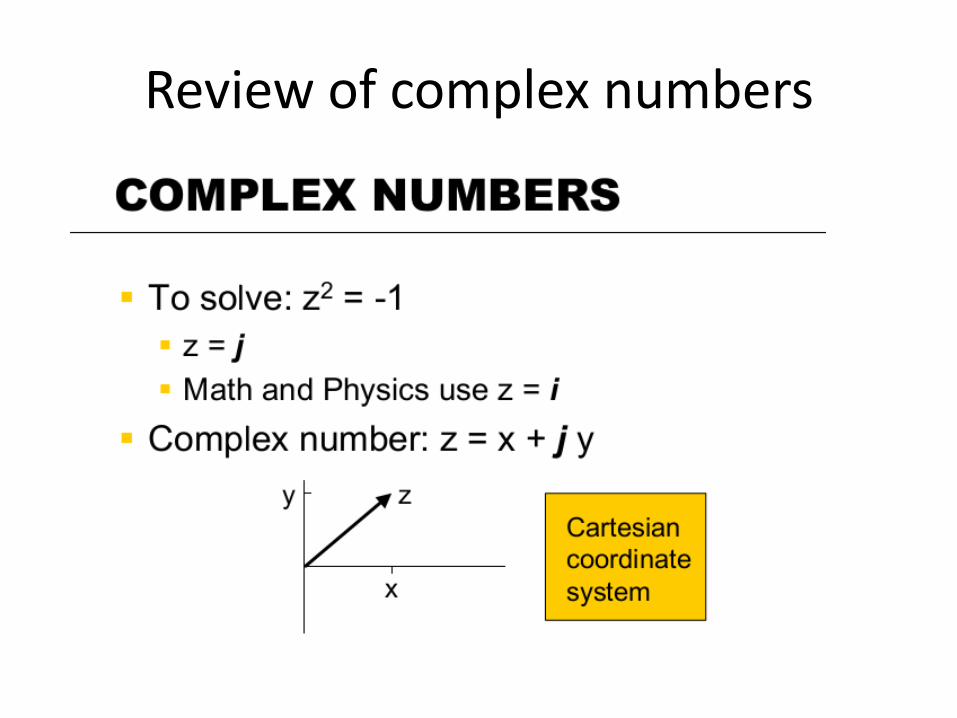
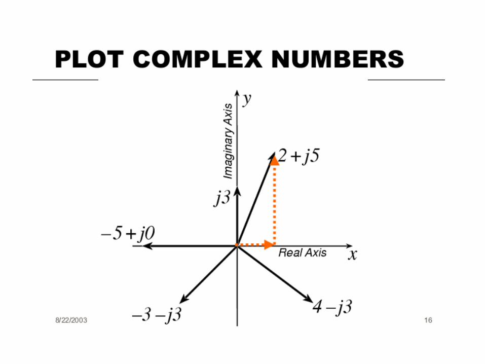
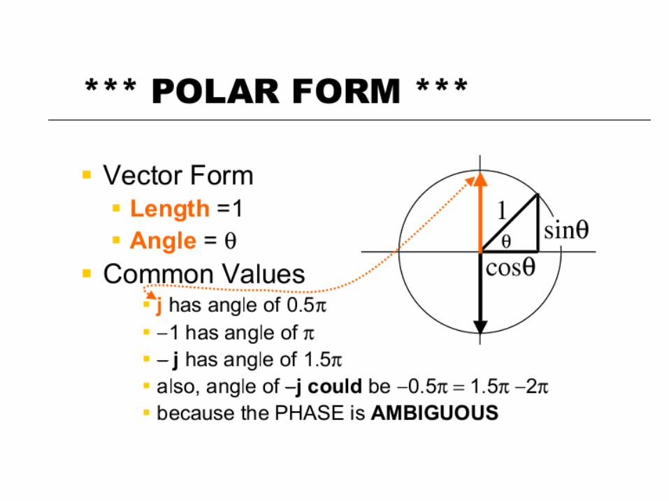
Review of complex numbers

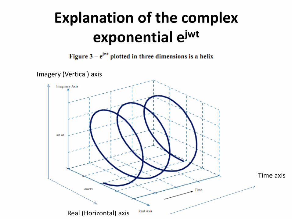
Explanation of the complex exponential ejwt

Time axis

Real (Horizontal) axis

Imagery (Vertical) axis

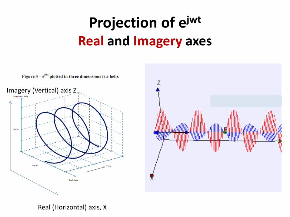
Projection of ejwt Real and Imagery axes

Real (Horizontal) axis, X

Imagery (Vertical) axis Z

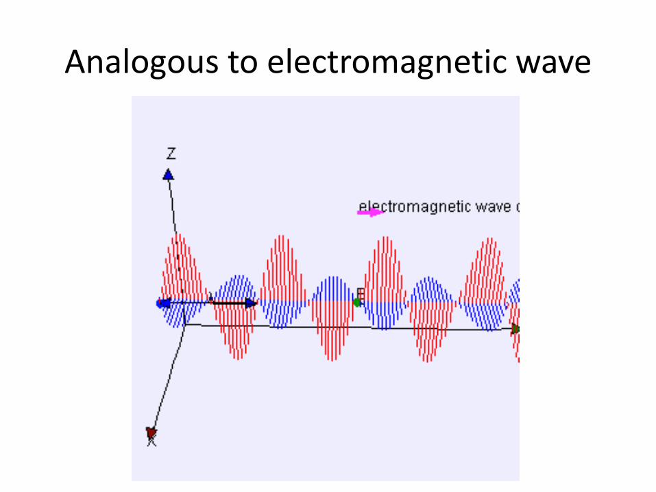
Analogous to electromagnetic wave

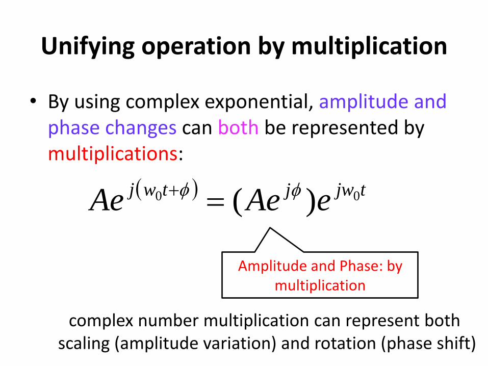
Unifying operation by multiplication

• By using complex exponential, amplitude and phase changes can both be represented by multiplications:

Amplitude and Phase: by multiplication

tjwjtwjeAeAe 00 )(

complex number multiplication can represent both scaling (amplitude variation) and rotation (phase shift)

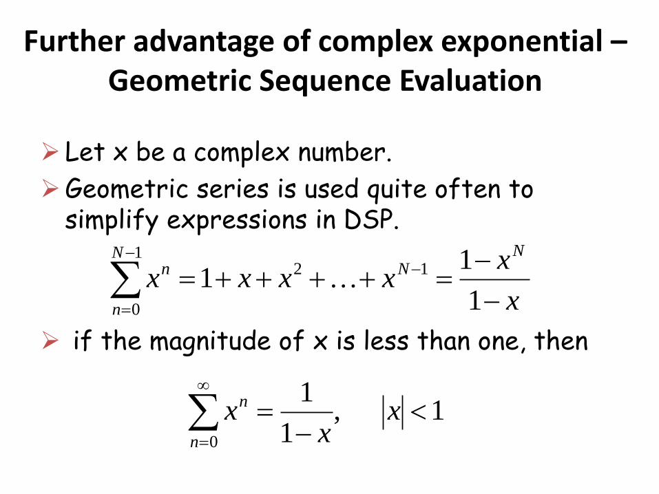
Further advantage of complex exponential – Geometric Sequence Evaluation

Let x be a complex number.

Geometric series is used quite often to simplify expressions in DSP.

if the magnitude of x is less than one, then

x

xxxxx

NN

n

Nn

1

11

1

0

12

1 ,1

1

0

xx

xn

n

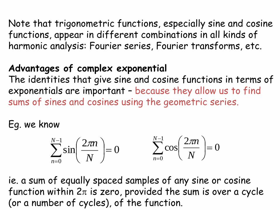
Note that trigonometric functions, especially sine and cosine functions, appear in different combinations in all kinds of harmonic analysis: Fourier series, Fourier transforms, etc. Advantages of complex exponential The identities that give sine and cosine functions in terms of exponentials are important – because they allow us to find sums of sines and cosines using the geometric series. Eg. we know ie. a sum of equally spaced samples of any sine or cosine function within 2 is zero, provided the sum is over a cycle (or a number of cycles), of the function.

1

0

02

sinN

n N

n

1

0

02

cosN

n N

n

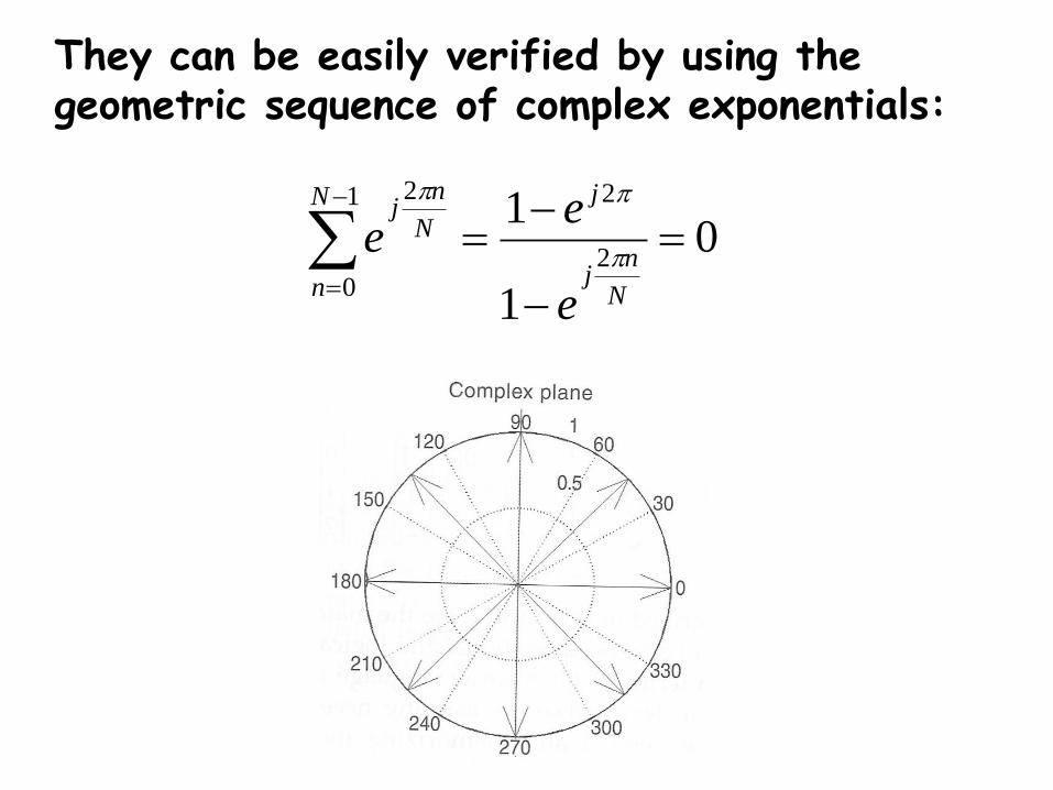
They can be easily verified by using the geometric sequence of complex exponentials:

0

1

11

02

22

N

n N

nj

j

N

nj

e

ee