Embed Size (px)
Citation preview
1/19/18
1
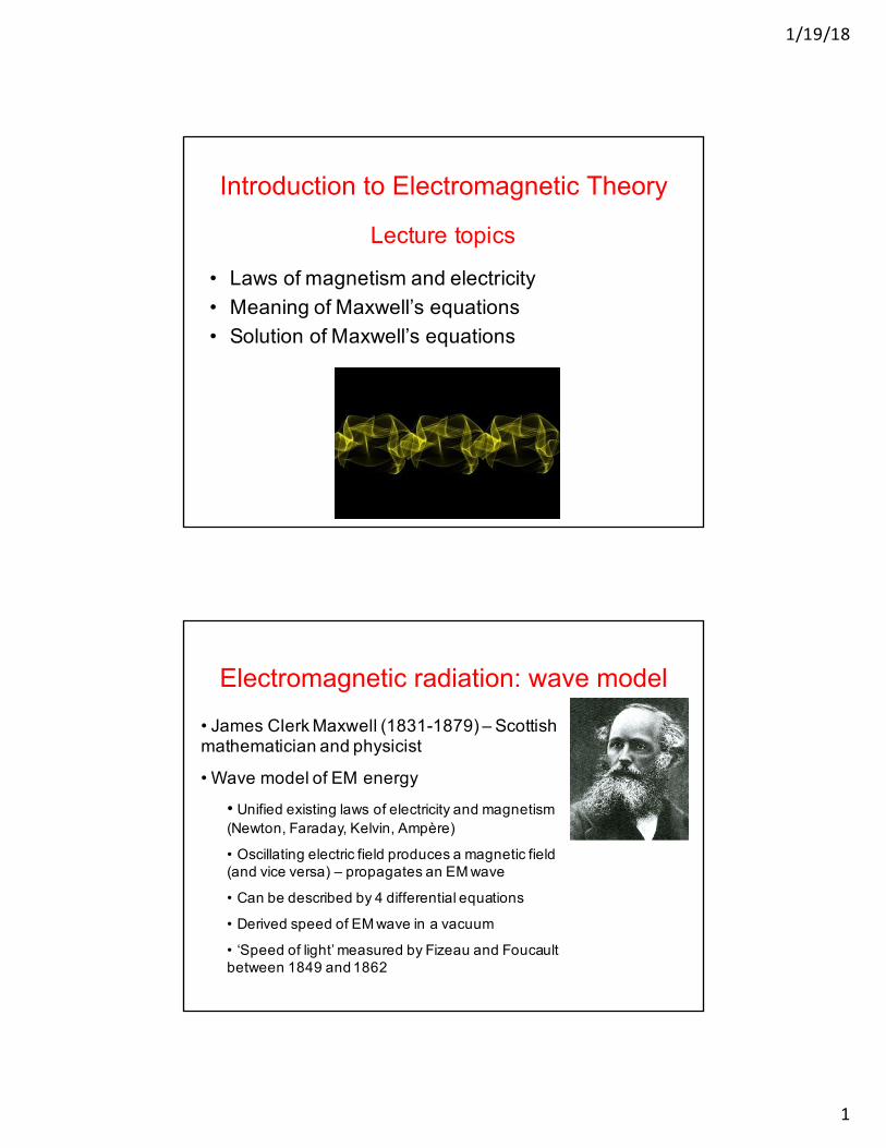
Lecture topics
• Laws of magnetism and electricity• Meaning of Maxwell’s equations• Solution of Maxwell’s equations
Introduction to Electromagnetic Theory
Electromagnetic radiation: wave model
• James Clerk Maxwell (1831-1879) – Scottish mathematician and physicist
• Wave model of EM energy
• Unified existing laws of electricity and magnetism (Newton, Faraday, Kelvin, Ampère)
• Oscillating electric field produces a magnetic field (and vice versa) – propagates an EM wave
• Can be described by 4 differential equations
• Derived speed of EM wave in a vacuum
• ‘Speed of light’ measured by Fizeau and Foucault between 1849 and 1862
1/19/18
2
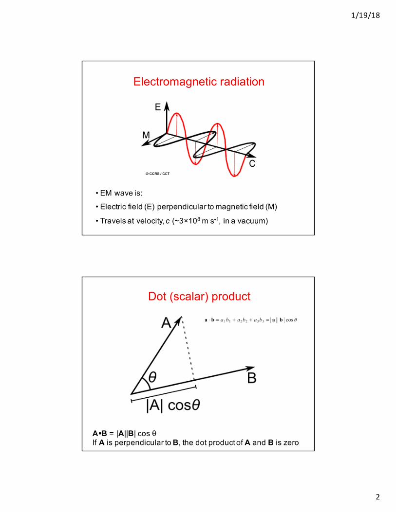
Electromagnetic radiation
• EM wave is:
• Electric field (E) perpendicular to magnetic field (M)
• Travels at velocity, c (~3×10⁸ m s-1, in a vacuum)
Dot (scalar) product
A�B = |A||B| cos θIf A is perpendicular to B, the dot product of A and B is zero
1/19/18
3
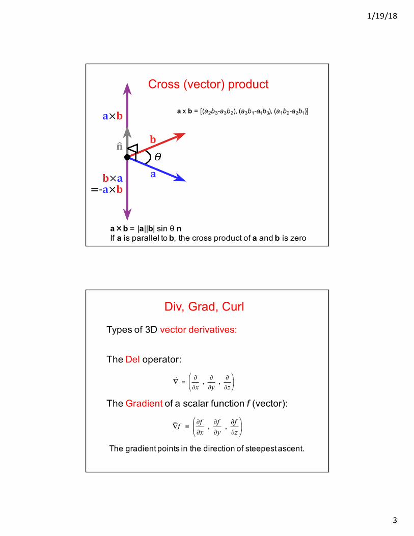
Cross (vector) product
a x b = [(a2b3-a3b2), (a3b1-a1b3), (a1b2-a2b1)]
a×b = |a||b| sin θ nIf a is parallel to b, the cross product of a and b is zero
Div, Grad, Curl
Types of 3D vector derivatives:
The Del operator:
The Gradient of a scalar function f (vector):
The gradient points in the direction of steepest ascent.
∇ ≡
∂∂x, ∂∂y, ∂∂z
$
%&
'
()
∇f ≡
∂f∂x, ∂f∂y, ∂f∂z
$
%&
'
()
1/19/18
4
Div, Grad, Curl
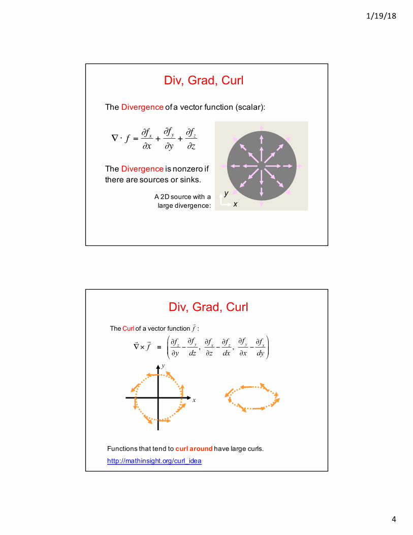
The Divergence of a vector function (scalar):
yx zff ff
x y z∂∂ ∂
∇⋅ ≡ + +∂ ∂ ∂
rr
The Divergence is nonzero if there are sources or sinks.
A 2D source with a large divergence: x
y€
∇ ⋅ f =∂fx∂x
+∂fy∂y
+∂fz∂z
Div, Grad, CurlThe Curl of a vector function
f :
∇×f ≡
∂f z∂y
−∂f ydz,∂f x∂z
−∂f zdx,∂f y∂x
−∂f xdy
&
'((
)
*++
Functions that tend to curl around have large curls.
http://mathinsight.org/curl_idea
x
y
1/19/18
5
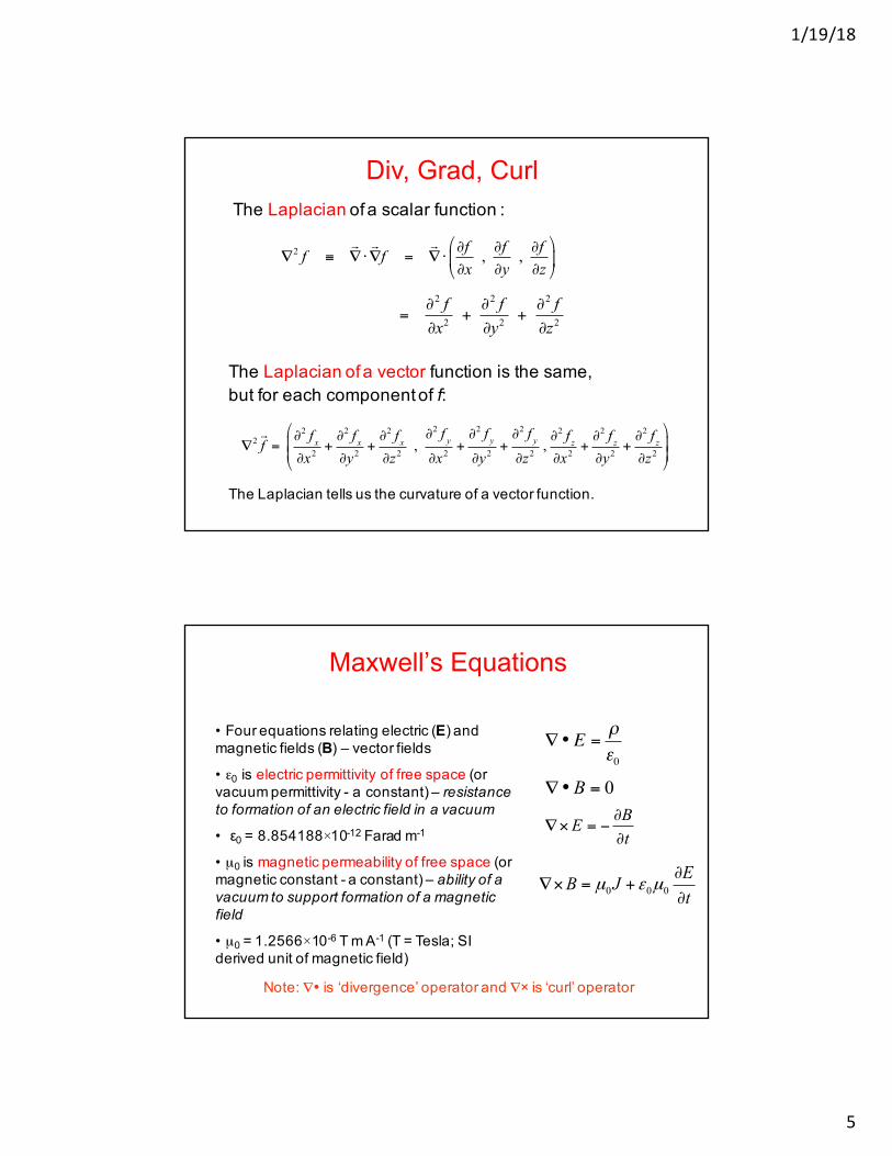
Div, Grad, CurlThe Laplacian of a scalar function :
The Laplacian of a vector function is the same, but for each component of f:
∇2 f ≡∇⋅∇f =
∇⋅
∂f∂x, ∂f∂y, ∂f∂z
%
&'
(
)*
2 2 2
2 2 2
f f fx y z∂ ∂ ∂
= + +∂ ∂ ∂
∇2f = ∂2 f x
∂x2+∂2 f x∂y2
+∂2 f x∂z2
,∂2 f y∂x2
+∂2 f y∂y2
+∂2 f y∂z2
,∂2 f z∂x2
+∂2 f z∂y2
+∂2 f z∂z2
#
$%%
&
'((
The Laplacian tells us the curvature of a vector function.
Maxwell’s Equations
• Four equations relating electric (E) and magnetic fields (B) – vector fields
• ε0 is electric permittivity of free space (or vacuum permittivity - a constant) – resistance to formation of an electric field in a vacuum
• ε0 = 8.854188×10⁻¹² Farad m-1
• µ0 is magnetic permeability of free space (or magnetic constant - a constant) – ability of a vacuum to support formation of a magnetic field
• µ0 = 1.2566×10⁻⁶ T m A-1 (T = Tesla; SI derived unit of magnetic field)
€
∇ • E =ρε0
tBE∂
∂−=×∇
0=•∇ B
tEJB∂
∂+=×∇ 000 µεµ
Note: ∇• is ‘divergence’ operator and ∇× is ‘curl’ operator
1/19/18
6
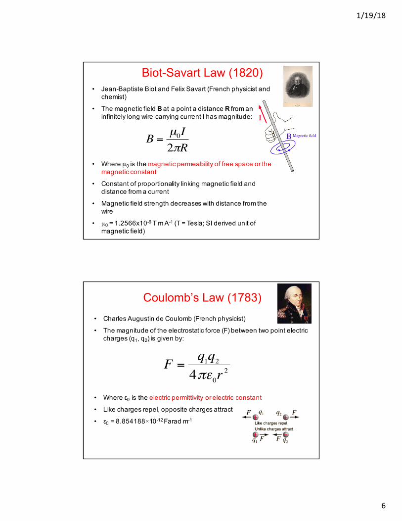
Biot-Savart Law (1820)• Jean-Baptiste Biot and Felix Savart (French physicist and
chemist)
• The magnetic field B at a point a distance R from an infinitely long wire carrying current I has magnitude:
• Where µ0 is the magnetic permeability of free space or the magnetic constant
• Constant of proportionality linking magnetic field and distance from a current
• Magnetic field strength decreases with distance from the wire
• µ0 = 1.2566x10⁻⁶ T m A-1 (T = Tesla; SI derived unit of magnetic field)
€
B =µ0I2πR
Coulomb’s Law (1783)• Charles Augustin de Coulomb (French physicist)
• The magnitude of the electrostatic force (F) between two point electric charges (q1, q2) is given by:
• Where ε0 is the electric permittivity or electric constant
• Like charges repel, opposite charges attract
• ε0 = 8.854188×10⁻¹² Farad m-1
€
F =q1q24πε0r
2
1/19/18
7
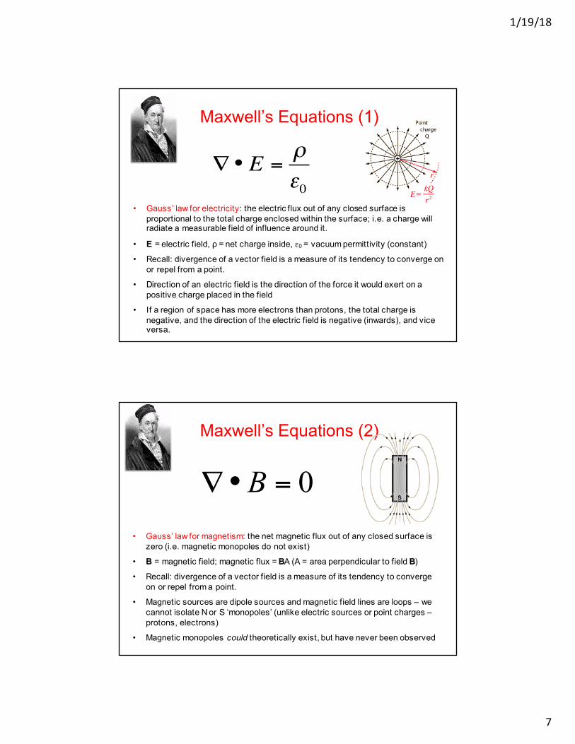
Maxwell’s Equations (1)
• Gauss’ law for electricity: the electric flux out of any closed surface is proportional to the total charge enclosed within the surface; i.e. a charge will radiate a measurable field of influence around it.
• E = electric field, ρ = net charge inside, ε0 = vacuum permittivity (constant)
• Recall: divergence of a vector field is a measure of its tendency to converge on or repel from a point.
• Direction of an electric field is the direction of the force it would exert on a positive charge placed in the field
• If a region of space has more electrons than protons, the total charge is negative, and the direction of the electric field is negative (inwards), and vice versa.
€
∇ • E =ρε0
Maxwell’s Equations (2)
• Gauss’ law for magnetism: the net magnetic flux out of any closed surface is zero (i.e. magnetic monopoles do not exist)
• B = magnetic field; magnetic flux = BA (A = area perpendicular to field B)
• Recall: divergence of a vector field is a measure of its tendency to converge on or repel from a point.
• Magnetic sources are dipole sources and magnetic field lines are loops – we cannot isolate N or S ‘monopoles’ (unlike electric sources or point charges –protons, electrons)
• Magnetic monopoles could theoretically exist, but have never been observed
0=•∇ B
1/19/18
8
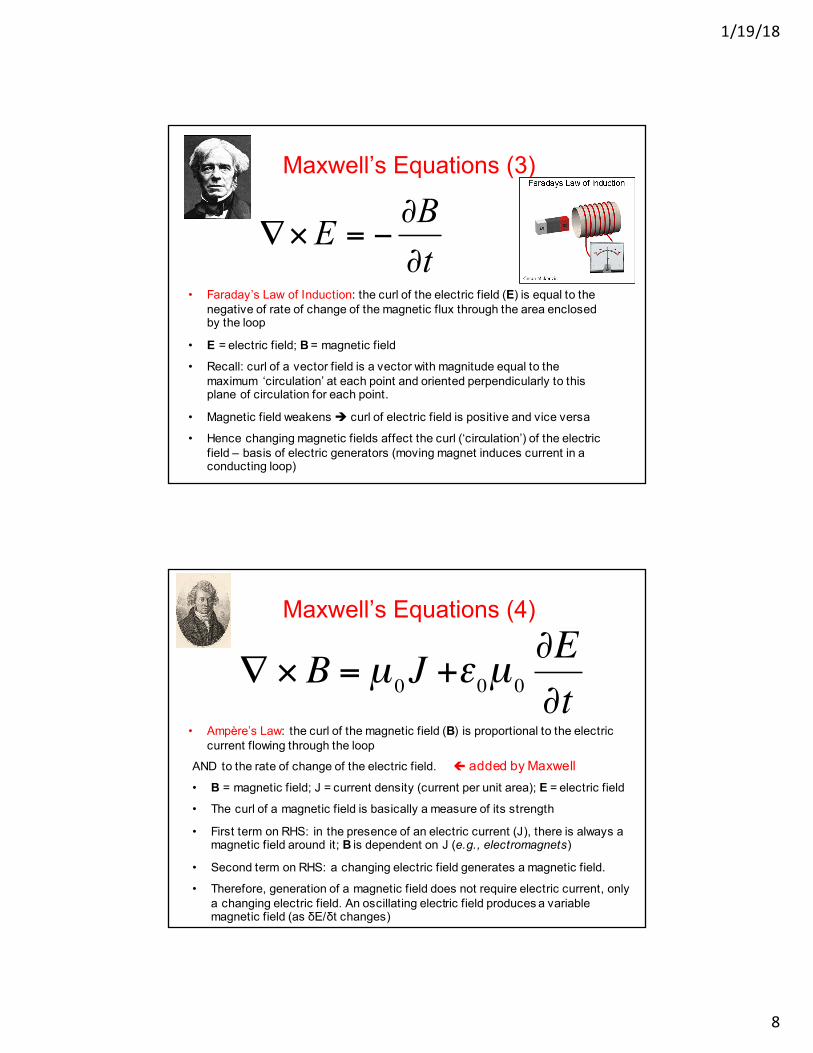
Maxwell’s Equations (3)
• Faraday’s Law of Induction: the curl of the electric field (E) is equal to the negative of rate of change of the magnetic flux through the area enclosed by the loop
• E = electric field; B = magnetic field
• Recall: curl of a vector field is a vector with magnitude equal to the maximum ‘circulation’ at each point and oriented perpendicularly to this plane of circulation for each point.
• Magnetic field weakens è curl of electric field is positive and vice versa
• Hence changing magnetic fields affect the curl (‘circulation’) of the electric field – basis of electric generators (moving magnet induces current in a conducting loop)
tBE∂
∂−=×∇
Maxwell’s Equations (4)
• Ampère’s Law: the curl of the magnetic field (B) is proportional to the electric current flowing through the loop
€
∇ × B = µ 0J
€
+ε0µ 0
∂E∂t
AND to the rate of change of the electric field. ç added by Maxwell• B = magnetic field; J = current density (current per unit area); E = electric field
• The curl of a magnetic field is basically a measure of its strength
• First term on RHS: in the presence of an electric current (J), there is always a magnetic field around it; B is dependent on J (e.g., electromagnets)
• Second term on RHS: a changing electric field generates a magnetic field.
• Therefore, generation of a magnetic field does not require electric current, only a changing electric field. An oscillating electric field produces a variable magnetic field (as δE/δt changes)
1/19/18
9
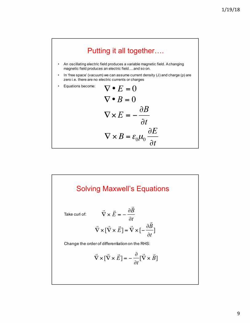
Putting it all together….• An oscillating electric field produces a variable magnetic field. A changing
magnetic field produces an electric field….and so on.
• In ‘free space’ (vacuum) we can assume current density (J) and charge (ρ) are zero i.e. there are no electric currents or charges
• Equations become:
€
∇ • E = 0
tBE∂
∂−=×∇
0=•∇ B
€
∇ × B = ε0µ0∂E∂t
Solving Maxwell’s Equations
Take curl of:
Change the order of differentiation on the RHS:
∇×E = −
∂B∂t
∇× [
∇×E] =
∇× [− ∂
B∂t
]
∇× [
∇×E] = − ∂
∂t[∇×B]
1/19/18
10
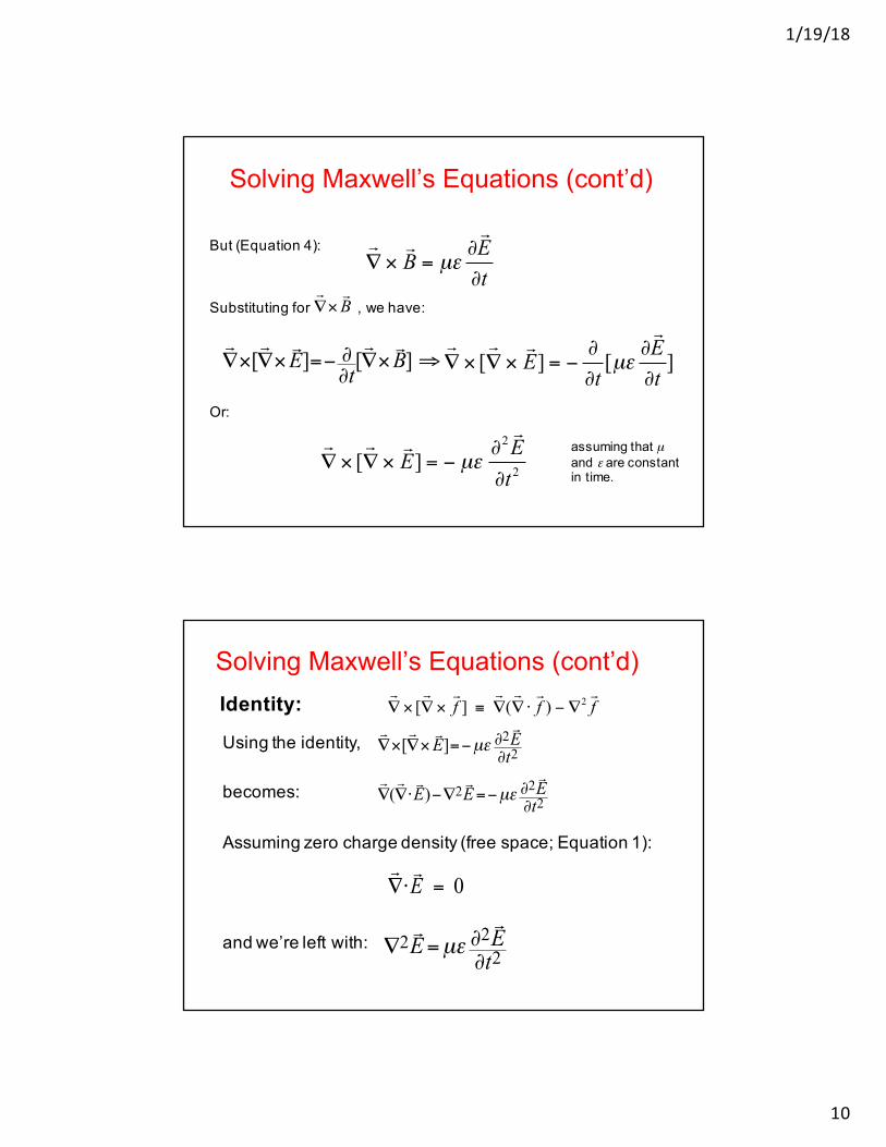
Solving Maxwell’s Equations (cont’d)
But (Equation 4):
Substituting for , we have:
Or:
∇× [
∇×E] = − ∂
∂t[µε ∂
E∂t
]
∇× [
∇×E] = − µε ∂
2E
∂t2
∇×[∇×E]=− ∂
∂t[∇×B] ⇒
assuming that µand ε are constant in time.
∇×B = µε
∂E∂t
∇×B
Solving Maxwell’s Equations (cont’d)
Using the identity,
becomes:
Assuming zero charge density (free space; Equation 1):
and we’re left with:
∇×[∇×E]=−µε ∂2
E
∂t2
∇(∇⋅E)−∇2
E=−µε ∂2
E
∂t2
∇⋅E = 0
∇2E=µε ∂2
E
∂t2
Identity: ∇× [
∇×f ] ≡
∇(∇⋅f ) − ∇2
f
1/19/18
11
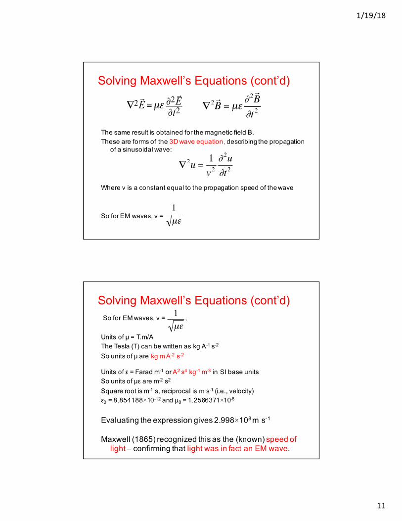
Solving Maxwell’s Equations (cont’d)
The same result is obtained for the magnetic field B.These are forms of the 3D wave equation, describing the propagation
of a sinusoidal wave:
Where v is a constant equal to the propagation speed of the wave
So for EM waves, v =
∇2E=µε ∂2
E
∂t2
€
∇2u =1v 2∂ 2u∂t 2
€
∇2 B = µε∂ 2 B
∂t 2
€
1µε
Solving Maxwell’s Equations (cont’d)So for EM waves, v = ,
Units of μ = T.m/AThe Tesla (T) can be written as kg A-1 s-2
So units of μ are kg m A-2 s-2
Units of ε = Farad m-1 or A2 s4 kg-1 m-3 in SI base unitsSo units of με are m-2 s2
Square root is m-1 s, reciprocal is m s-1 (i.e., velocity)ε0 = 8.854188×10⁻¹² and μ0 = 1.2566371×10⁻⁶
Evaluating the expression gives 2.998×10⁸ m s-1
Maxwell (1865) recognized this as the (known) speed of light – confirming that light was in fact an EM wave.
€
1µε
1/19/18
12
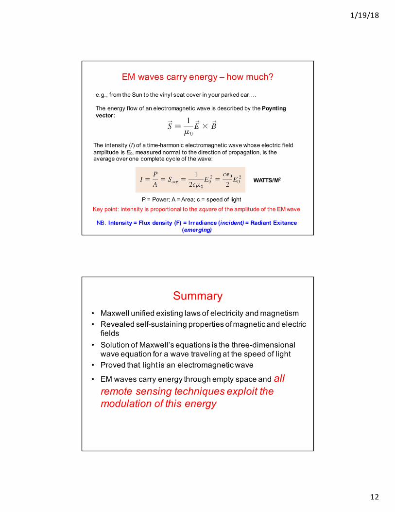
e.g., from the Sun to the vinyl seat cover in your parked car….
The energy flow of an electromagnetic wave is described by the Poyntingvector:
EM waves carry energy – how much?
The intensity (I) of a time-harmonic electromagnetic wave whose electric field amplitude is E0, measured normal to the direction of propagation, is the average over one complete cycle of the wave:
WATTS/M2
Key point: intensity is proportional to the square of the amplitude of the EM wave
NB. Intensity = Flux density (F) = Irradiance (incident) = Radiant Exitance(emerging)
P = Power; A = Area; c = speed of light
Summary• Maxwell unified existing laws of electricity and magnetism• Revealed self-sustaining properties of magnetic and electric
fields• Solution of Maxwell’s equations is the three-dimensional
wave equation for a wave traveling at the speed of light• Proved that light is an electromagnetic wave
• EM waves carry energy through empty space and all remote sensing techniques exploit the modulation of this energy
1/19/18
13
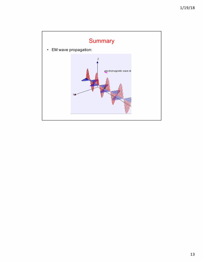
Summary• EM wave propagation: