Introduction to geodetic VLBI

David MayerAndreas Hellerschmied

Johannes BöhmHarald Schuh and Johannes Böhm, Very Long Baseline Interferometry for Geodesy and Astrometry, in Guochang Xu (editor): Sciences of Geodesy II, Innovations and Future Developments, Springer Verlag, ISBN 978-3-642-27999-7, doi: 10.1007/978-3-642-28000-9, pp. 339-376, 2013.

What is Geodesy

Geodesy is the science of accurately measuring and understanding the Earth's geometric shape, orientation in space, and gravity field.

Why use VLBI for geodesy?• It is the only technique which is able to position the

earth in space (estimate all 5 EOP)• Intercontinental baselines (tectonic motion)• Provides scale factor for the TRF• Provides very accurate source position (CRF)

Difference astronomic and geodetic VLBI

• Astronomic VLBI interested in imaging sources etc.

• Geodetic VLBI interested in parameters of the Earth– Sources are used as static reference points in the sky– Stable, point-like and radio loud quasars are used– Observations to these sources are used to estimate

geodetic parameters, such as station coordinates, etc.

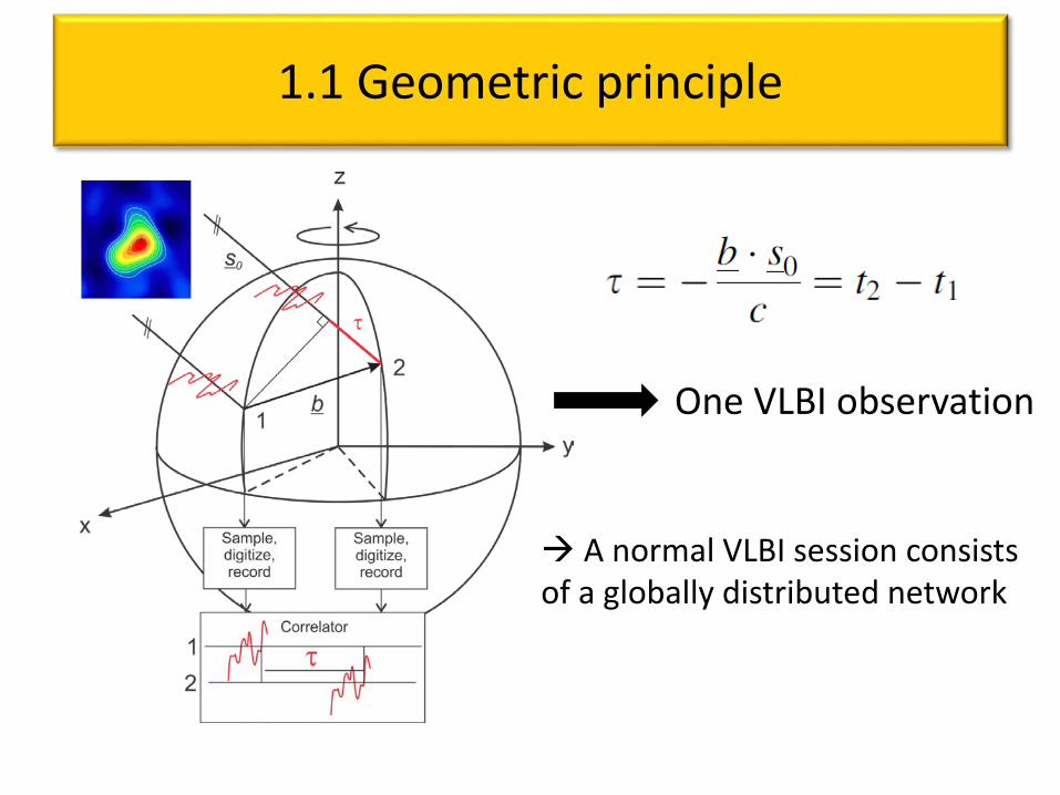
1.1 Geometric principle

A normal VLBI session consists of a globally distributed network

One VLBI observation

1.2 Data acquisition

• VLBI observation plans (schedules) define which sources are observed by which stations at which time

• Scheduling for Geodesy– Typically 24h sessions with globally distributed station

network observed in S- and X-Band simultaneously– Packages SKED (Vandenberg 1999) or VieVS (Sun et al. 2014)– All observations to one source at a time form a ‘scan’– Different integration and slewing times need to be

considered– It is important to have as many observations as possible

1.2 Data acquisition

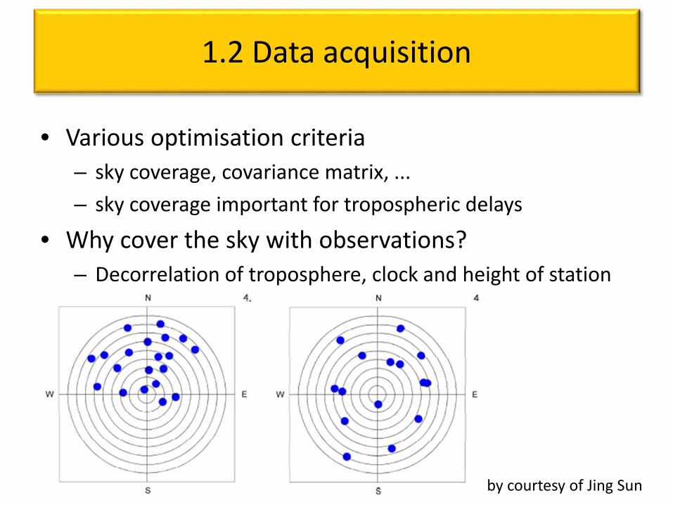
• Various optimisation criteria– sky coverage, covariance matrix, ...– sky coverage important for tropospheric delays

• Why cover the sky with observations?– Decorrelation of troposphere, clock and height of station

by courtesy of Jing Sun

1.3 Correlation

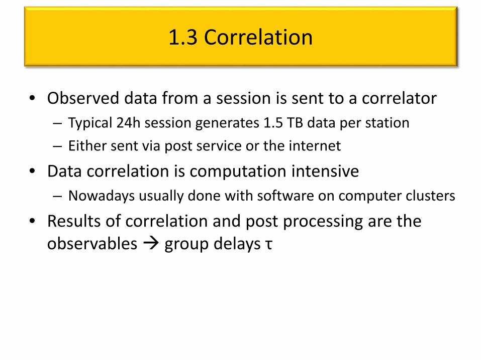
• Observed data from a session is sent to a correlator– Typical 24h session generates 1.5 TB data per station– Either sent via post service or the internet

• Data correlation is computation intensive– Nowadays usually done with software on computer clusters

• Results of correlation and post processing are the observables group delays τ

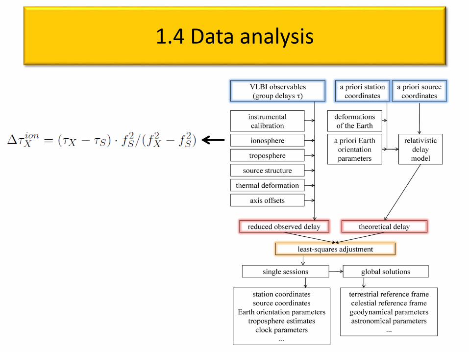
1.4 Data analysis

1.4 Data analysis

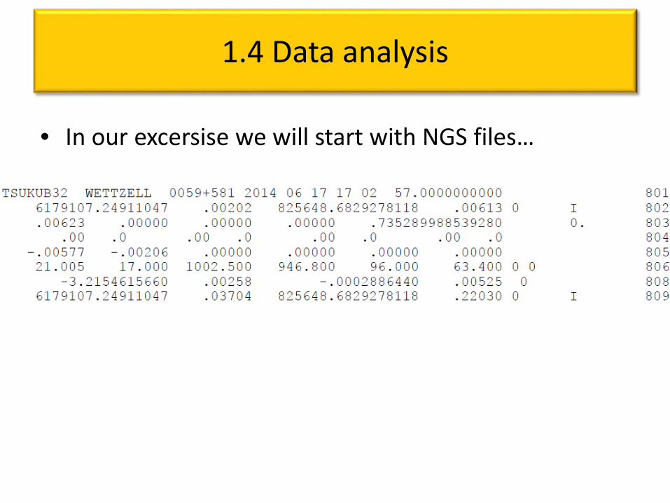
• In our excersise we will start with NGS files…

2. Theoretical delays

• Before calculating the observed – computed (o – c) value, various models need to be applied

• IERS Conventions (Petit and Luzum 2010)• IVS Conventions, e.g. thermal deformation

2.1 Station coordinates

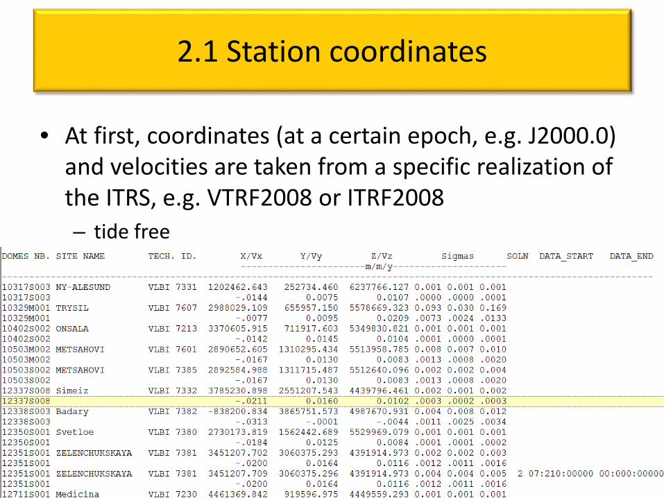
• At first, coordinates (at a certain epoch, e.g. J2000.0) and velocities are taken from a specific realization of the ITRS, e.g. VTRF2008 or ITRF2008– tide free

2.1 Station coordinates

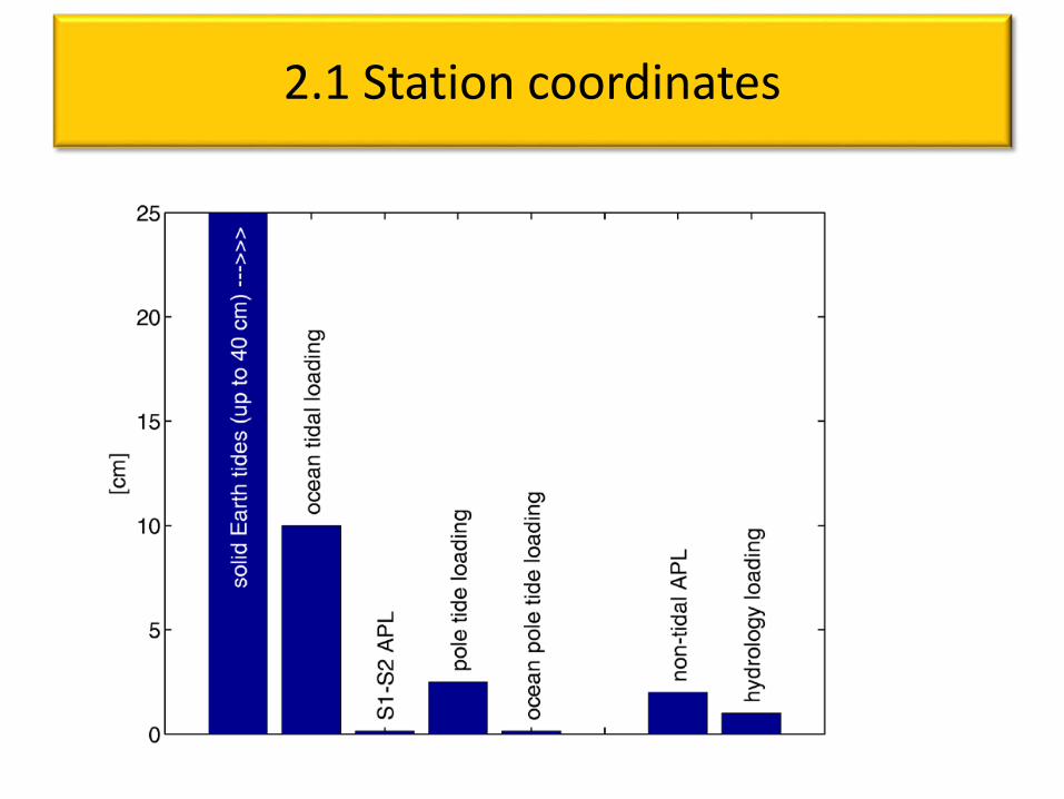
• Periodic corrections to get closer to true coordinates– solid Earth tides– ocean tide loading– (ocean) pole tide loading– tidal atmosphere loading (S1 and S2)

2.1 Station coordinates

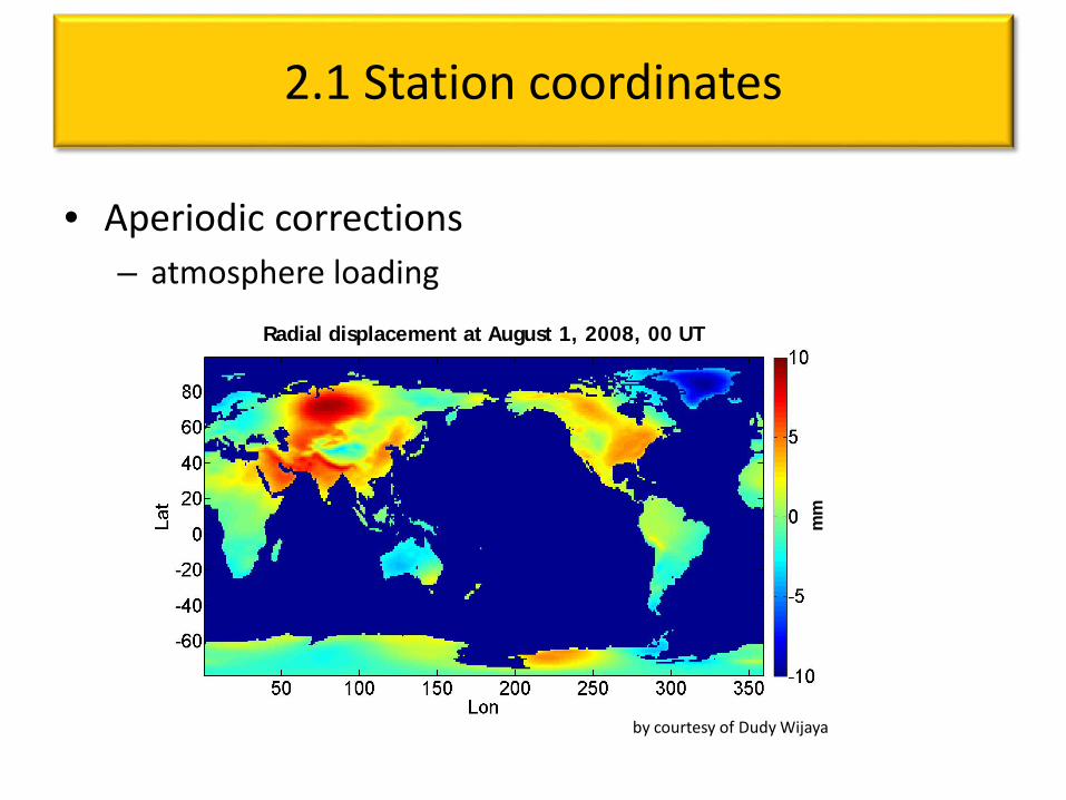
• Aperiodic corrections– atmosphere loading

Radial displacement at August 1, 2008, 00 UT

mm

by courtesy of Dudy Wijaya

2.1 Station coordinates

• Aperiodic corrections– atmosphere loading– ocean non-tidal loading– hydrology loading

2.1 Station coordinates

2.2 Earth orientation

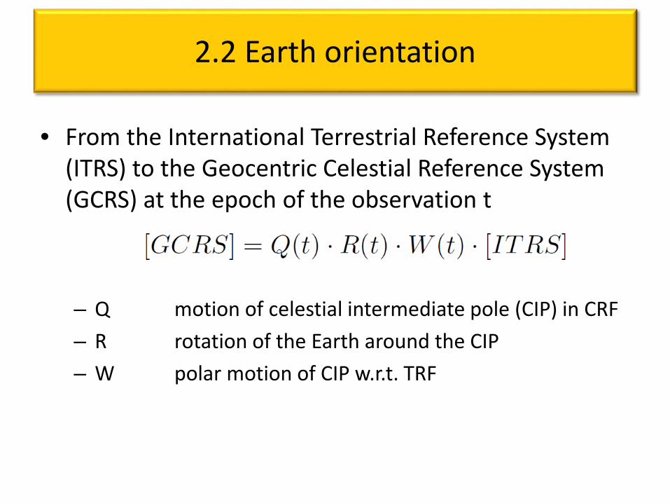
• From the International Terrestrial Reference System (ITRS) to the Geocentric Celestial Reference System (GCRS) at the epoch of the observation t

– Q motion of celestial intermediate pole (CIP) in CRF– R rotation of the Earth around the CIP– W polar motion of CIP w.r.t. TRF

2.2 Earth orientation

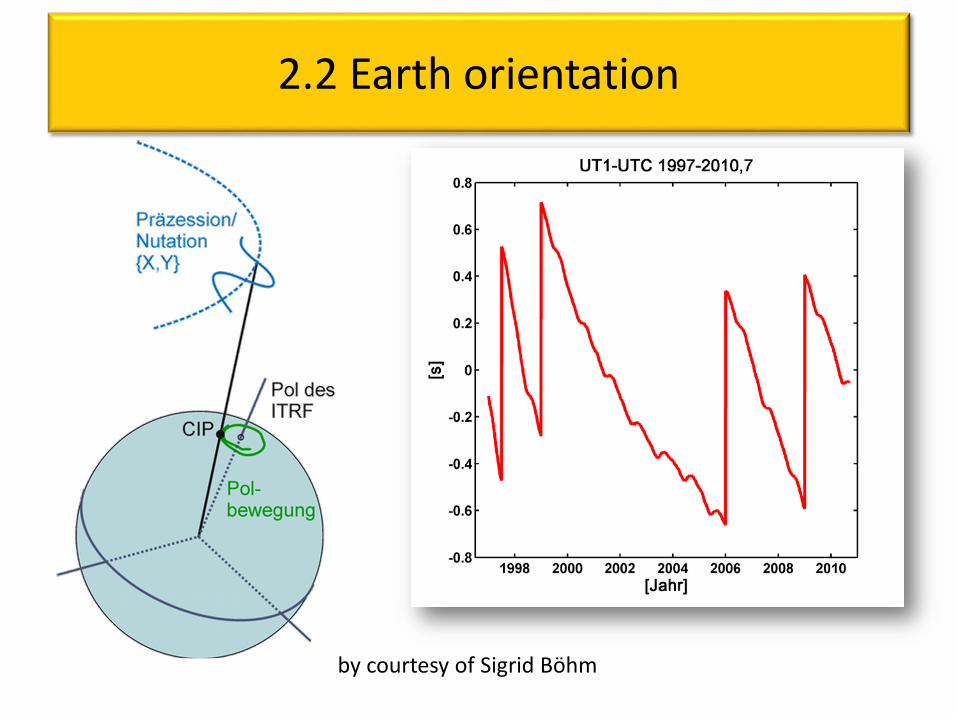
by courtesy of Sigrid Böhm

2.2 Earth orientation

• Celestial pole offsets, UT1 – UTC, polar motion need to be observed

• Daily values provided by the IERS to be used as a priori information

• Models for diurnal and sub-diurnal ocean tides• Libration (forced polar motion)

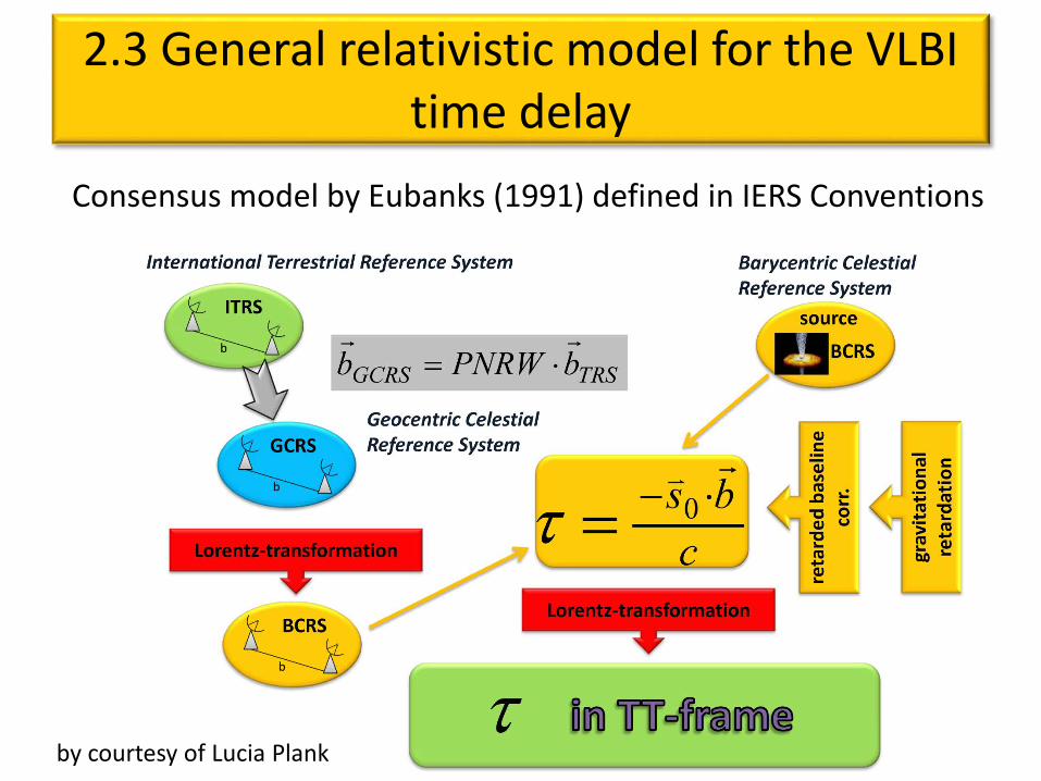
2.3 General relativistic model for the VLBI time delay

by courtesy of Lucia Plank

Consensus model by Eubanks (1991) defined in IERS Conventions

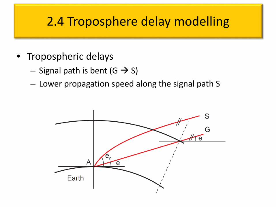
2.4 Troposphere delay modelling

• Tropospheric delays– Signal path is bent (G S)– Lower propagation speed along the signal path S

2.4 Troposphere delay modelling

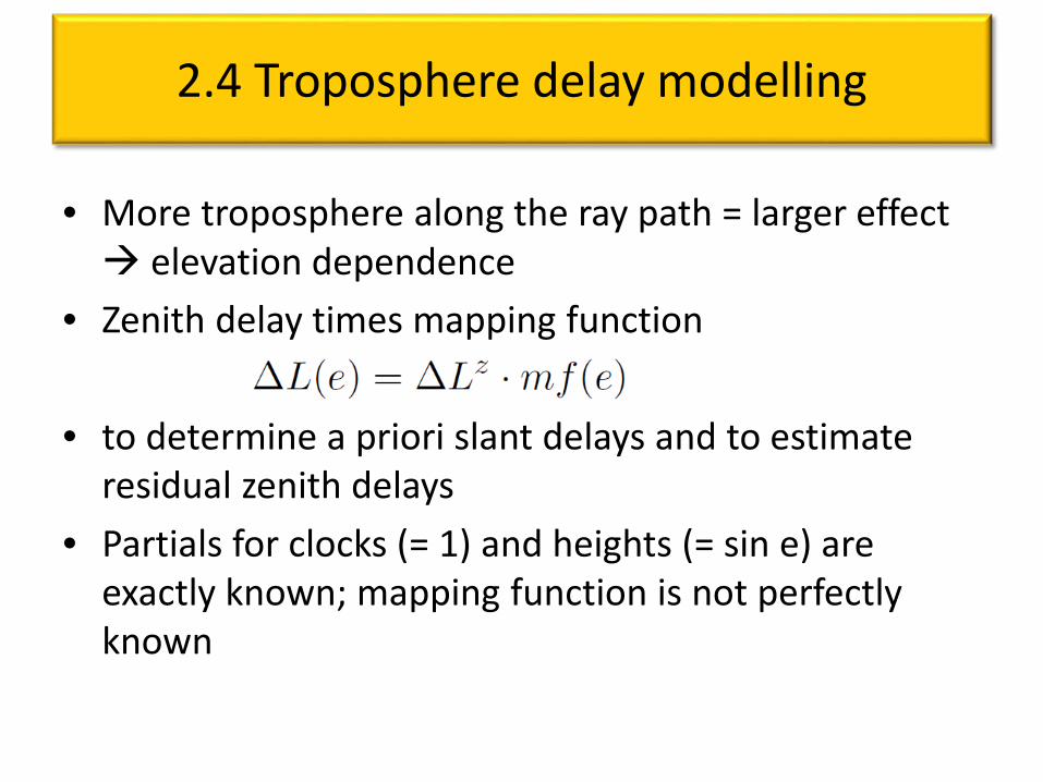
• More troposphere along the ray path = larger effect elevation dependence

• Zenith delay times mapping function

• to determine a priori slant delays and to estimate residual zenith delays

• Partials for clocks (= 1) and heights (= sin e) are exactly known; mapping function is not perfectly known

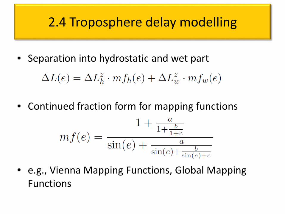
2.4 Troposphere delay modelling

• Separation into hydrostatic and wet part

• Continued fraction form for mapping functions

• e.g., Vienna Mapping Functions, Global Mapping Functions

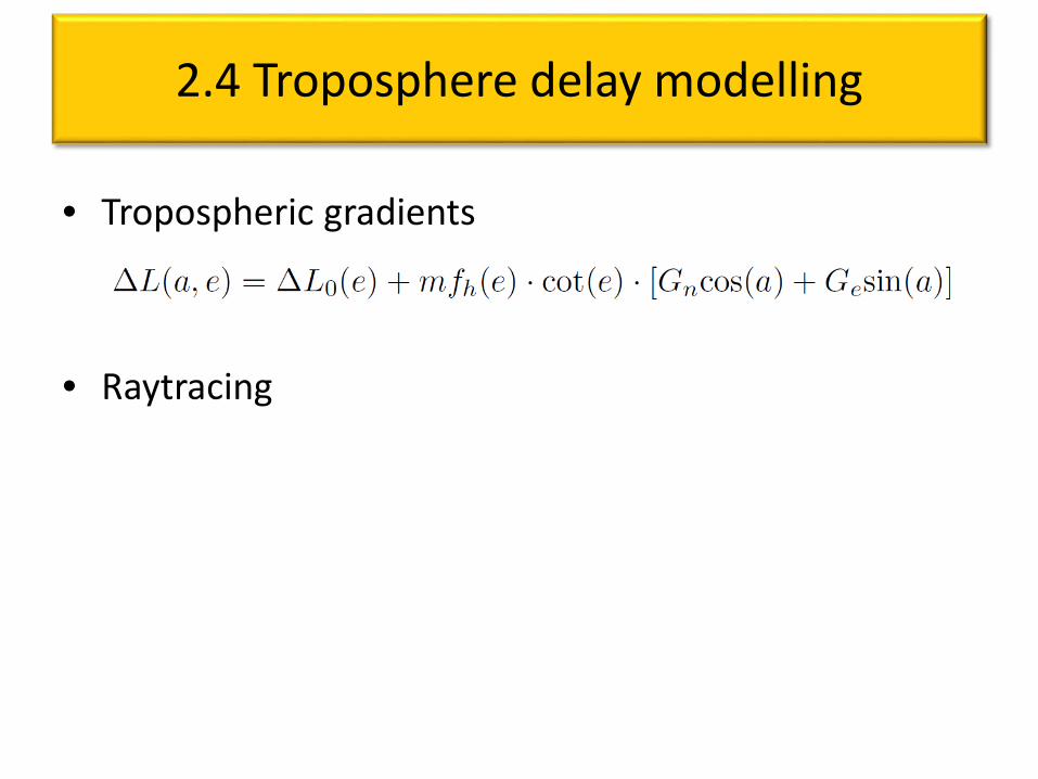
2.4 Troposphere delay modelling

• Tropospheric gradients

• Raytracing

2.5 Antenna deformation

• Snow and ice loading• Gravitational deformation• Thermal deformation

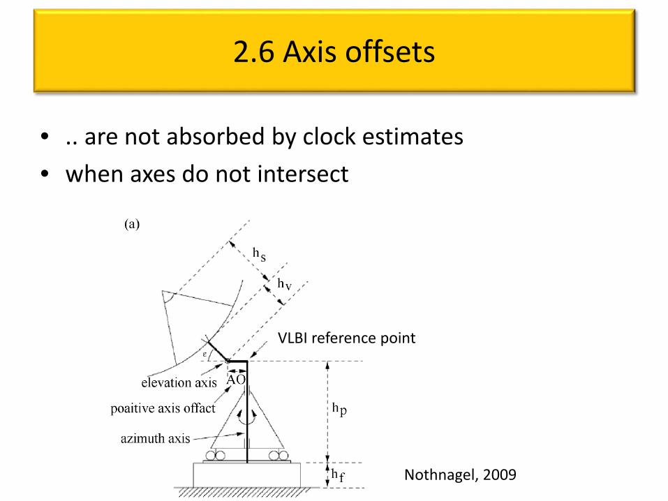
2.6 Axis offsets

• .. are not absorbed by clock estimates• when axes do not intersect

Nothnagel, 2009

VLBI reference point

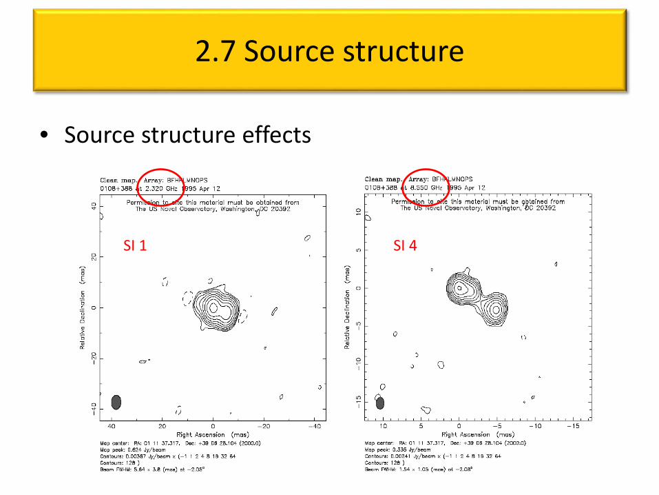
2.7 Source structure

• Source structure effects

SI 1 SI 4

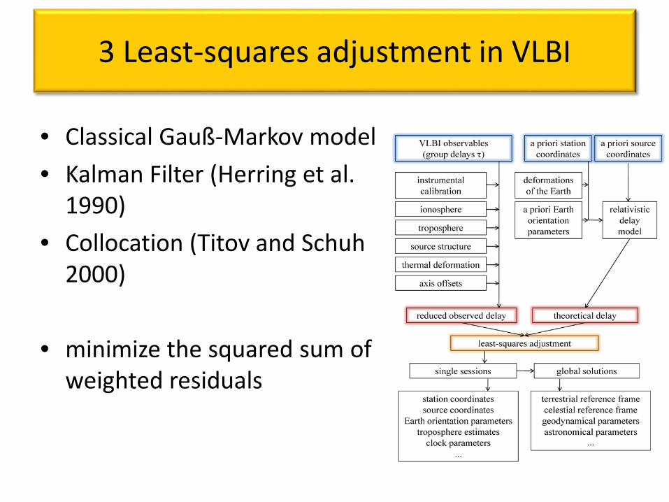
3 Least-squares adjustment in VLBI

• Classical Gauß-Markov model• Kalman Filter (Herring et al.

1990)• Collocation (Titov and Schuh

2000)

• minimize the squared sum of weighted residuals

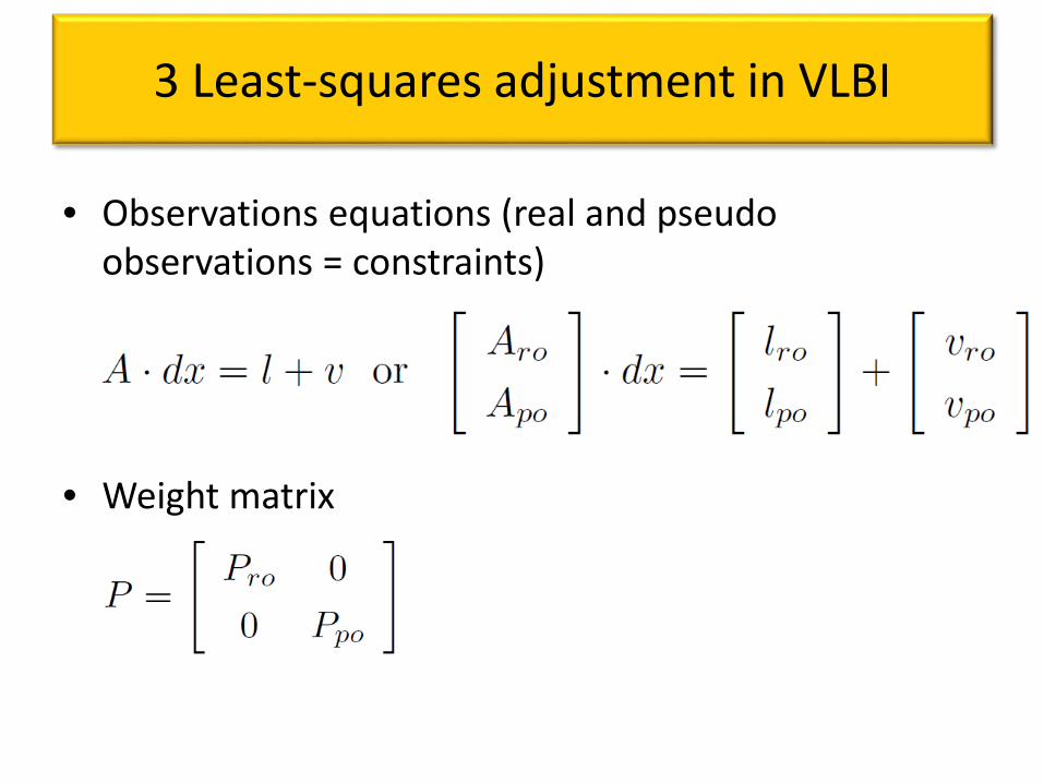
3 Least-squares adjustment in VLBI

• Observations equations (real and pseudo observations = constraints)

• Weight matrix

3 Least-squares adjustment in VLBI

• Auxiliary parameters: clocks (quadratic functions plus piecewise linear offsets; reference clock), zenith wet delays and gradients

• Clock breaks• Piecewise linear offsets at e.g. integer hours• .. allows combination with other space geodetic

techniques at normal equation level

3 Least-squares adjustment in VLBI

• Many other geodetic/astrometric parameters to be estimated

• E.g., Earth orientation parameters can be estimated daily or with higher time resolution

3 Least-squares adjustment in VLBI

• Global VLBI solutions from a (large) number of single solutions

• E.g., for station and source coordinates• Often, auxiliary parameters are removed (= implicitly

estimated)

3 Least-squares adjustment in VLBI

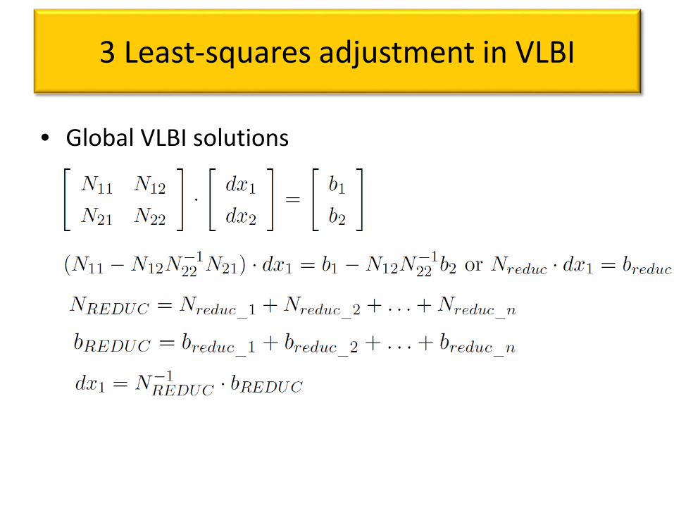
• Global VLBI solutions

3 Least-squares adjustment in VLBI

Conditions to prevent N matrix from being singular• free networks need a datum• rank deficiency is six (scale is defined by

observations)• NNR/NNT usually applied• Episodic changes need to be considered

(instrumental changes, Earthquakes)

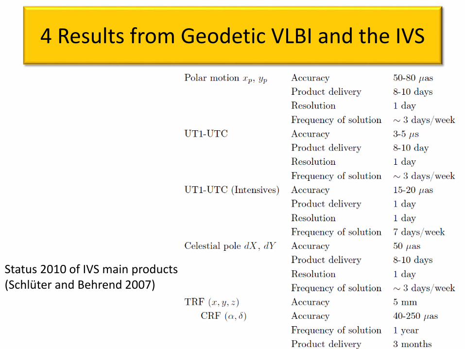
4 Results from Geodetic VLBI and the IVS

Status 2010 of IVS main products (Schlüter and Behrend 2007)