Introduction to Geometry

it is a draft of lecture notes of H.M. Khudaverdian.Manchester, 18 May 2011

Contents

1 Euclidean space 31.1 Vector space. . . . . . . . . . . . . . . . . . . . . . . . . . . . 31.2 Basic example of n-dimensional vector space—Rn . . . . . . . 41.3 Linear dependence of vectors . . . . . . . . . . . . . . . . . . . 41.4 Dimension of vector space. Basis in vector space. . . . . . . . 71.5 Scalar product. Euclidean space . . . . . . . . . . . . . . . . . 91.6 Orthonormal basis in Euclidean space . . . . . . . . . . . . . . 111.7 Transition matrices. Orthogonal bases and orthogonal matrices 12

1.7.1 Linear operators and transition matrices . . . . . . . . 151.8 Orthogonal 2× 2 matrices . . . . . . . . . . . . . . . . . . . . 151.9 Orientation in vector space . . . . . . . . . . . . . . . . . . . . 181.10 †Linear operator in E3 preservinig orientation is a rotation . . 231.11 Vector product in oriented E3 . . . . . . . . . . . . . . . . . . 25

1.11.1 Vector product—area of parallelogram . . . . . . . . . 281.11.2 Area of parallelogram in E2 and determinant of 2 × 2

matrices . . . . . . . . . . . . . . . . . . . . . . . . . . 291.11.3 Volume of parallelepiped . . . . . . . . . . . . . . . . 31

2 Differential forms in E2 and E3 322.1 Tangent vectors, curves, velocity vectors on the curve . . . . . 322.2 Reparameterisation . . . . . . . . . . . . . . . . . . . . . . . . 332.3 0-forms and 1-forms . . . . . . . . . . . . . . . . . . . . . . . . 35

2.3.1 Vectors—directional derivatives of functions . . . . . . 37

1

2.4 Differential 1-form in arbitrary coordinates . . . . . . . . . . 402.4.1 Calculations in arbitrary coordinates ∗ . . . . . . . . . 402.4.2 Calculations in polar coordinates . . . . . . . . . . . . 42

2.5 Integration of differential 1-forms over curves . . . . . . . . . . 442.6 Integral over curve of exact form . . . . . . . . . . . . . . . . . 472.7 † Differential 2-forms in E2 . . . . . . . . . . . . . . . . . . . . 48

2.8 0-forms (functions)d−→ 1-forms

d−→ 2-forms . . . . . . . . . . 492.9 †Exact and closed forms . . . . . . . . . . . . . . . . . . . . . 502.10 †Integration of two-forms. Area of the domain . . . . . . . . . 50

3 Curves in E3. Curvature 523.1 Curves. Velocity and acceleration vectors . . . . . . . . . . . . 523.2 Behaviour of acceleration vector under reparameterisation . . 543.3 Length of the curve . . . . . . . . . . . . . . . . . . . . . . . 563.4 Natural parameterisation of the curves . . . . . . . . . . . . . 563.5 Curvature. Curvature of curves in E2 and E3 . . . . . . . . . . 593.6 Curvature of curve in an arbitrary parameterisation. . . . . . . 60

4 Surfaces in E3. Curvatures and Shape operator. 634.1 Coordinate basis, tangent plane to the surface. . . . . . . . . . 644.2 Curves on surfaces. Length of the curve. Internal and external

point of the view. First Quadratic Form . . . . . . . . . . . . 654.3 Unit normal vector to surface . . . . . . . . . . . . . . . . . . 684.4 † Curves on surfaces—normal acceleration and normal curvature 704.5 Shape operator on the surface . . . . . . . . . . . . . . . . . . 714.6 Principal curvatures, Gaussian and mean curvatures and shape

operator . . . . . . . . . . . . . . . . . . . . . . . . . . . . . . 734.7 Shape operator, Gaussian and mean curvature for sphere and

cylinder . . . . . . . . . . . . . . . . . . . . . . . . . . . . . . 754.8 †Principal curvatures and normal curvature . . . . . . . . . . . 77

5 Parallel transport. Geometrical meaning of Gaussian curva-ture 795.1 Concept of parallel transport of the vector tangent to the surface 795.2 Geometrical meaning of Gaussian curvature. Theorema Egregium 81

2

6 †Appendices 836.1 Formulae for vector fields and differentials in cylindrical and

spherical coordinates . . . . . . . . . . . . . . . . . . . . . . . 836.2 Curvature and second order contact (touching) of curves . . . 856.3 Integral of curvature over planar curve. . . . . . . . . . . . . 876.4 Relations between usual curvature normal curvature and geodesic

curvature. . . . . . . . . . . . . . . . . . . . . . . . . . . . . . 906.5 Normal curvature of curves on cylinder surface. . . . . . . . . 926.6 Parallel transport of vectors tangent to the sphere. . . . . . . 936.7 Parallel transport along a closed curve on arbitrary surface. . . 966.8 Gauss Bonnet Theorem . . . . . . . . . . . . . . . . . . . . . . 966.9 A Tale on Differential Geometry . . . . . . . . . . . . . . . . 99

1 Euclidean space

We recall important notions from linear algebra.

1.1 Vector space.

Vector space V on real numbers is a set of vectors with operations ” +”—addition of vector and ” · ”—multiplication of vector Lon real number(sometimes called coefficients, scalars). These operations obey the followingaxioms

• ∀a,b ∈ V, a+ b ∈ V ,

• ∀λ ∈ R, ∀a ∈ V, λa ∈ V .

• ∀a,ba+ b = b+ a (commutativity)

• ∀a,b, c, a+ (b+ c) = (a+ b) + c (associativity)

• ∃ 0 such that ∀a a+ 0 = a

• ∀a there exists a vector −a such that a+ (−a) = 0.

• ∀λ ∈ R, λ(a+ b) = λa+ λb

• ∀λ, µ ∈ R(λ+ µ)a = λa+ µa

3

• (λµ)a = λ(µa)

• 1a = a

It follows from these axioms that in particularly 0 is unique and −a isuniquely defined by a. (Prove it.)

Examples of vector spaces...

1.2 Basic example of n-dimensional vector space—Rn

A basic example of vector space (over real numbers) is a space of orderedn-tuples of real numbers.R2 is a space of pairs of real numbers. R2 = (x, y), x, y ∈ RR3 is a space of triples of real numbers. R3 = (x, y, z), x, y, z ∈ RR4 is a space of quadruples of real numbers. R4 = (x, y, z, t), x, y, z, t,∈ R

and so on...Rn—is a space of n-typles of real numbers:

Rn = (x1, x2, . . . , xn), x1, . . . , , xn ∈ R (1.1)

If x,y ∈ Rn are two vectors, x = (x1, . . . , xn), y = (y1, . . . , yn) then

x+ y = (x1 + y1, . . . , xn + yn) .

and multiplication on scalars is defined as

λx = λ · (x1, . . . , xn) = (λx1, . . . , λxn) , (λ ∈ R) .

(λ ∈ R).

1.3 Linear dependence of vectors

We often consider linear combinations in vector space:∑i

λixi = λ1x1 + λ2x2 + · · ·+ λmxm , (1.2)

where λ1, λ2, . . . , λm are coefficients (real numbers), x1,x2, . . . ,xm are vectorsfrom vector space V .

4

We say that linear combination (1.2) is trivial if all coefficients λ1, λ2, . . . , λmare equal to zero.

λ1 = λ2 = · · · = λm = 0 .

We say that linear combination (1.2) is not trivial if at least one of coef-ficients λ1, λ2, . . . , λm is not equal to zero:

λ1 = 0, orλ2 = 0, or . . . orλm = 0 .

Recall definition of linearly dependent and linearly independent vectors:Definition The vectors x1,x2, . . . ,xm in vector space V are linearly

dependent if there exists a non-trivial linear combination of these vectorssuch that it is equal to zero.

In other words we say that the vectors x1,x2, . . . ,xm in vector space Vare linearly dependent if there exist coefficients µ1, µ2, . . . , µm such that atleast one of these coefficients is not equal to zero and

µ1x1 + µ2x2 + · · ·+ µmxm = 0 . (1.3)

Respectively vectors x1,x2, . . . ,xm are linearly independent if they arenot linearly dependent. This means that an arbitrary linear combination ofthese vectors which is equal zero is trivial.

In other words vectors x1,x2,xm are linearly independent if the condi-tion

µ1x1 + µ2x2 + · · ·+ µmxm = 0

implies that µ1 = µ2 = · · · = µm = 0.Very useful and workableProposition Vectors x1,x2, . . . ,xm in vector space V are linearly

dependent if and only if at least one of these vectors is expressed via linearcombination of other vectors:

xi =∑j =i

λjxj . (1.4)

Proof. If the condition (1.4) is obeyed then xi −∑

j =i λjxj = 0. Thisnon-trivial linear combination is equal to zero. Hence vectors x1, . . . ,xmare linearly dependent.

Now suppose that vectors x1, . . . ,xm are linearly dependent. Thismeans that there exist coefficients µ1, µ2, . . . , µm such that at least one of

5

these coefficients is not equal to zero and the sum (1.3) equals to zero. WLOGsuppose that µ1 = 0. We see that to

x1 = −µ2

µ1

x2 −µ3

µ1

x3 − · · · − µm

µ1

xm ,

i.e. vector x1 is expressed as linear combination of vectors x2,x3, . . . ,xm .

Formulate and give a proof of usefulLemma Let m vectors x1,x2, . . . ,xm belong to the span of n vectors

a1, a2, . . . , an, i.e. every vector xi (i = 1, . . . ,m) can be expressed as alinear combination of vectors a1, a2, . . . , an:

x1 = λ11a1 + λ21a2 + · · ·+ λn1an

x2 = λ12a1 + λ22a2 + · · ·+ λn2an

x3 = λ13a1 + λ23a2 + · · ·+ λn3an

. . .

xm = λ1ma1 + λ2ma2 + · · ·+ λnman

(1.5)

Then vectors x1,x2, . . . ,xm are linearly dependent if m > n.

ProofProve using mathematical induction. If n = 1 then the statement is obvious: it

follows from (1.5) that all vectors xi are proportional to vector a1. Hence they are linearlydependent, since they are proportional each other.

Let a statement be true for m = k. Prove it for m = k + 1.Consider the first equation

x1 = λ11a1 + λ2

1a2 + · · ·+ λk1ak + λk+1

1 ak+1 (1.6)

If vector x1 = 0 then nothing to prove: vectors 0,x2,x3, . . . ,xm are linearly depen-dent. If x1 = 0 then one of the coefficients in (1.6) is not equal to zero. WLOG sup-pose that λ1

k+1 = 0. Hence ak+1 can be expressed as a linear combination of vectorsx1,a1,a2, . . . ,ak:

ak+1 = x1 −λ11

λk+11

a1 −λ21

λk+11

a2 − · · · − λk1

λk+11

ak

Input this expansion of ak+1 in expressions in (1.5) for vectors x2,x3, . . . ,xm. We will seethat m− 1 vectors

x′2 = x2 − λk+1

2 x1,x′3 = x3 − λk+1

3 x1 . . . ,x′m = xm − λk+1

m x1 (1.7)

are expressed as linear combinations of k vectors a1,a2, . . . ,ak. Hence due to inductivehypothesis vectors x′

2,x′3, . . . ,x

′m are linearly dependent:

µ2x′2 + · · ·+ µmx′

m = µ2(x2 − λk+12 x1) + · · ·+ µm(xm − λk+1

m x1) = 0,

6

where one of coefficients µ2, . . . , µm is not equal to zero. Now it follows from (1.7) that

this is non-trivial combination of vectors x1, . . . ,xm, i.e. vectors x1, . . . ,xm are linearly

dependent.

1.4 Dimension of vector space. Basis in vector space.

Definition Vector space V has a dimension n if there exist n linearly inde-pendent vectors in this vector space, and any n+ 1 vectors in V are linearlydependent.

In the case if in the vector space V there exist n linearly independent vectors for an

arbitrary natural number n then the space V is infinite-dimensional

BasisRecall that we say that vector space V is spanned by vectors x1, . . . ,xn

(or vectors vectors x1, . . . ,xn span vector space V ) if any vector a ∈ Vcan be expresses as a linear combination of vectors x1, . . . ,xn.

Basis is a set of linearly independent vectors in vector space V which span(generate) vector space V . More in detail:

Definition Let V be n-dimensional vector space. The ordered set e1, e2, . . . , enof n linearly independent vectors in V is called a basis (an ordered basis) ofthe vector space V .

Proposition 1 Let e1, . . . , en be an arbitrary basis in n-dimensionalvector space V . Then any vector a ∈ V can be expressed as a linear combi-nation of vectors e1, . . . , en in a unique way, i.e. for every vector x ∈ Vthere exist a set an ordered set of coefficients a1, . . . , an such that

x = x1e1 + · · ·+ xnen (1.8)

and if

x = a1e1 + · · ·+ anen = b1e1 + · · ·+ bnen , (1.9)

then a1 = b1, a2 = b2, . . . , an = bn. In other words for any vector x ∈ V thereexists an ordered n-tuple (x1, . . . , xn) of coefficients such that x =

∑ni=1 x

ieiand this n-tuple is unique.

Proof Let x be an arbitrary vector in vector space V . The dimension ofvector space V equals to n. Hence n + 1 vectors (e1, . . . , en,x) are linearlydependent: λ1e1+ · · ·+λnen+λn+1x = 0 and this combination is non-trivial.

7

If λn+1 = 0 then λ1e1+ · · ·+λnen = 0 and this combination is non-trivial, i.e.vectors (e1, . . . , en are linearly dependent. Contradiction. Hence λn+1 = 0,i.e. vector x can be expressed via vectors (e1, . . . , en): x = x1e1 + . . . xnenwhere xi = − λi

λn+1. We prove that any vector can be expressed via vectors

of basis. Prove now uniqueness. This expansion is unique. Indeed if (1.9)holds then (a1 − b1)e1 + (a2 − b2)e2 + · · · + (an − bn)en = 0. Due to linearindependence of basis vectors

this means that (a1 − b1) = (a2 − b2) = · · · = (an − bn) = 0, i.e. a1 =b1, a2 = b2, . . . , an = bn

Definition Coefficients a1, . . . , an are called components of the vectorx in the basis e1, . . . , en or just shortly components of the vector x.

Another very useful and workable statement

Proposition 2 Let e1, . . . , em be an ordered set of vectors in vectorspace V such that an arbitrary vector x ∈ V can be expressed as a linearcombination of vectors e1, . . . , en in a unique way (see (1.8) and (1.9)above). Then

• V is a finite-dimensional space of dimension m.

• e1, . . . , em is a basis in this space.

This is very practical statement: it can be often used to find a dimensionof vector space.

Remark We say ”a basis” not ”the basis”, since there are many bases inthe vector space V . (See below and also Homework 1).

Proof. Show first that the vectors e1, . . . , em are linearly independent. Let µ1e1 +µ2 + · · · + µmem = 0. This relation holds if µ1 = µ2 = µ3 = · · · = µm = 0. Due tothe uniqueness of the expansion applied to the vector x = 0 we see that µ1e1 + µ2 +· · · + µmem = 0 implies that µ1 = µ2 = µ3 = · · · = µm = 0. Hence vectors e1, . . . , emare linearly independent. We proved that dimV ≥ m. Consider an arbitrary m + 1vectors x1,x2, . . . ,xm+1. For any of these vectors xi vectors xi, e1, . . . , em are linearlydependent and vectors e1, . . . , em are linearly independent. Hence any of vectors xi canbe expressed as a linear combination of vectors e1, . . . , em. Thus we proved that anym + 1 vectors in V belong to the space of vectors e1, . . . , em. Hence according to thelemma in the subsection 1.2 of lecture notes any m+1 vectors in V are linearly dependent.Thus we proved that dimV = m.

The ordered set e1, . . . , em is a set ofm linearly independent vectors inm-dimensionalvector space V . Hence e1, . . . , em is a basis.

Remark Basis is a maximal set of linearly independent vectors in a linear space V .

8

Canonical basis in Rn

We considered above the basic example of n-dimensional vector space—aspace of ordered n-tuples of real numbers: Rn = (x1, x2, . . . , xn), xi ∈ R(see the subsection 1.2). What is the meaning of letter n in the definition ofRn?

Consider vectors e1, e2, . . . , en ∈ Rn:

e1 = (1, 0, 0 . . . , 0, 0)e2 = (0, 1, 0 . . . , 0, 0). . . . . .en = (0, 0, 0 . . . , 0, 1)

(1.10)

Then for an arbitrary vector Rn ∋ a = (a1, a2, a3, . . . , an)

a = (a1, a2, a3, . . . , an) =

a1(1, 0, 0 . . . , 0, 0)+a2(0, 1, 0 . . . , 0, 0)+a3(0, 0, 1, 0 . . . , 0, 0)+· · ·+an(0, 1, 0 . . . , 0, 1) =

=m∑i=1

aiei = aiei (we will use sometimes condensed notations x = xiei)

Thus we see that for every vector a ∈ Rn we have unique expansion via thevectors (1.10). Thus according to Proposition 2 above the dimension of thespace Rn is equals to n and (1.10) is a basis in Rn.

Remark One can find another basis in Rn–just take an arbitrary orderedset of n linearly independent vectors. (See exercise 7 in Homework 1). Thebasis (1.10) is distinguished. Sometimes it is called canonical basis in Rn.

Remark One can consider a set of ordered n-tuples in Rn as the setof points. Two points a,b ∈ Rn define a vector: if a = (a1, . . . , an), b= (b1, . . . , bn), then the vector ab attached to the point a has coordinates= (b1 − a1, b2 − a2 . . . , bn − an) 1.

1.5 Scalar product. Euclidean space

In vector space one have additional structure: scalar product of vectors.

1Rn considered as a set of points is called affine space

9

Definition Scalar product in a vector space V is a function B(x,y)on a pair of vectors which takes real values and satisfies the the followingconditions:

B(x,y) = B(y,x) (symmetricity condition)B(λx+ µx′,y) = λB(x,y) + µB(x′,y) (linearity condition)(x,x) ≥ 0 , (x,x) = 0 ⇔ x = 0 (positive-definiteness condition)

(1.11)

Definition Euclidean space is a vector space equipped with a scalar product.

One can easy to see that the function B(x,y) is bilinear function, i.e. itis linear function with respect to the second argument also2. This followsfrom previous axioms:

B(x, λy+µy′) =︸︷︷︸symm.

B(λy+µy′,x) =︸︷︷︸linear.

λB(y,x)+µB(y′,x) =︸︷︷︸symm.

λB(x,y)+µB(x,y′) .

A bilinear function B(x,y) on pair of vectors is called sometimes bilinear form on

vector space. Bilinear form B(x,y) which satisfies the symmetricity condition is called

symmetric bilinear form. Scalar product is nothing but symmetric bilinear form on vectors

which is positive-definite: B(x,x) ≥ 0) and is non-degenerate ((x,x) = 0 ⇒ x = 0.

Example We considered the vector space Rn, the space of n-tuples (seethe subsection 1.2). One can consider the vector space Rn as Euclidean spaceprovided by the scalar product

B(x,y) = x1y1 + · · ·+ xnyn (1.12)

Exercise a) Check that it is indeed scalar product.Notations!Scalar product sometimes is called ”inner” product or ”dot” product.

Later on we will use for scalar product B(x,y) just shorter notation (x,y)or ⟨x,y⟩. Sometimes it is used for scalar product a notation x · y. Usuallythis notation is reserved only for the canonical case (1.12).

b) Show that operation (x,y) = x1y1+x2y2−x3y3 does not define scalarproduct in R3. (See also exercises in Homework 2)

2Here and later we will denote scalar product B(x,y) just by (x,y). Scalar productsometimes is called inner product. Sometimes it is called dot product.

10

1.6 Orthonormal basis in Euclidean space

One can see that for scalar product (1.12) and for the basis e1, . . . , endefined by the relation (1.10) the following relations hold:

(ei, ej) = δij =

1 if i = j

0 if i = j(1.13)

Let e1, e2, . . . , en be an ordered set of n vectors in n-dimensional Eu-clidean space which obeys the conditions (1.13). One can see that this orderedset is a basis 3.

Definition-Proposition The ordered set of vectors e1, e2, . . . , en inn-dimensional Euclidean space which obey the conditions (1.13) is a basis.This basis is called an orthonormal basis.

One can prove that every (finite-dimensional) Euclidean space possessesorthonormal basis. Later by default we consider only orthonormal bases inEuclidean spaces. Respectively scalar product will be defined by the formula(1.12).

Indeed let e1, e2, . . . , en be an orthonormal basis in Euclidean space.Then for an arbitrary two vectors x,y, such that x =

∑xiei, y =

∑yjej

we have:

(x,y) =(∑

xiei,∑

yjej

)=

n∑i,j=1

xiyj(ei, ej) =n∑

i,j=1

xiyjδij =n∑

i=1

xiyi

(1.14)We come to the scalar product (1.12). Later on we usually will considerscalar product defined by the formula (1.12) ((1.14)).

Length of the vectors, angle between vectorsThe scalar product of vector on itself defines the length of the vector:

Length of the vector x = |x| =√(x,x) =

√(x1)2 + · · ·+ (xn)2 (1.15)

If we consider Euclidean space En as the set of points then the distance

3Indeed prove that conditions (1.13) imply that these n vectors are linear independent.Suppose that λ1e1 + λ2e2 + · · ·+ λnen = 0. For an arbitrary i multiply the left and righthand sides of this relation on a vector ei. We come to condition λi = 0. Hence vectors(e1, e2, . . . , en) are linearly dependent.

11

between two points x,y is the length of corresponding vector:

distance between points x,y = |x− y| =√

(y1 − x1)2 + · · ·+ (yn − xn)2

(1.16)Geometrical properties of scalar product

We recall very important formula how scalar (inner) product is relatedwith the angle between vectors:

(x,y) = x1y1 + x2y2 = |x||y| cosφ (1.17)

where φ is an angle between vectors x and y in E2.This formula is valid also in the three-dimensional case and any n-dimensional

case for n ≥ 1. It gives as a tool to calculate angle between two vectors:

(x,y) = x1y1 + x2y2 + · · ·+ xnyn = |x||y| cosφ (1.18)

In particulary it follows from this formula that

angle between vectors x,y is acute if scalar product (x,y) is positiveangle between vectors x,y is obtuse if scalar product (x,y) is negativevectors x,y are perpendicular if scalar product (x,y) is equal to zero

(1.19)

|x| =√(x,x) (1.20)

Remark Geometrical intuition tells us that cosinus of the angle between two vectorshas to be less or equal to one and it is equal to one if and only if vectors x,y are collinear.Comparing with (1.18) we come to the inequality:

(x,y)2 =(x1y1 + · · ·+ xnyn

)2 ≤((x1)2 + · · ·+ (xn)2

) ((y1)2 + (· · ·+ (yn)2

)= (x,x)(y,y)

and(x,y)2 = (x,x)(y,y) if vectors are colienar, i.e. xi = λyi

(1.21)

This is famous Cauchy–Buniakovsky–Schwarz inequality, one of most important inequali-

ties in mathematics. (See for more details Homework 2)

1.7 Transition matrices. Orthogonal bases and orthog-onal matrices

One can consider different bases in vector space.

12

Let A be n× n matrix with real entries, A = ||aij||, i, j = 1, 2, . . . , n:

A =

a11 a12 . . . a1na21 a22 . . . a2na31 a32 . . . a3n. . . . . . . . . . . .

a(n−1) 1 a(n−1)2 . . . a(n−1)n

an 1 an2 . . . ann

Let e1, e2, . . . , en be an arbitrary basis in n-dimensional vector space V .

The basis e1, e2, . . . , en can be considered as row of vectors, or 1 × nmatrix with entries–vectors.

Multiplying 1 × n matrix e1, e2, . . . , en on matrix A we come to newrow of vectors e′1, e′2, . . . , e′n such that

e′1, e′2, . . . , e′n = e1, e2, . . . , enA = (1.22)

e′1, e′2, . . . , e′n = e1, e2, . . . , en

a11 a12 . . . a1na21 a22 . . . a2na31 a32 . . . a3n. . . . . . . . . . . .

a(n−1) 1 a(n−1)2 . . . a(n−1)n

an 1 an2 . . . ann

(1.23)

,

e′1 = a11e1 + a21e2 + a31e3 + · · ·+ a(n−1) 1en−1 + an 1en

e′1 = a12e1 + a22e2 + a32e3 + · · ·+ a(n−1) 2en−1 + an 2en

e′1 = a13e1 + a23e2 + a33e3 + · · ·+ a(n−1) 3en−1 + an 1en

· · · = . . . · · ·+ . . . · · ·+ . . . · · ·+ · · ·+ . . . . . . . . . . . .

e′n = a1ne1 + a2ne2 + a3ne3 + · · ·+ a(n−1)nen−1 + annen

(1.24)

or shortly:

e′i =n∑

k=1

ekaki .

What is the condition that the row e′1, e′2, . . . , e′n is a basis too? The rowe′1, e′2, . . . , e′n is a basis if and only if vectors (e′1, e

′2, . . . , e

′n) are linearly

independent. Thus we come to

13

Proposition 1 Let e1, e2, . . . , en be a basis in n-dimensional vectorspace V , and let A be an n×n matrix with real entries. Then e′1, e′2, . . . , e′n =e1, e2, . . . , enA is a basis if and only if the matrix A has rank n, i.e. it isnon-degenerate matrix.

We call matrix A a transition matrix from a basis e1, e2, . . . , en to thebasis e′1, e′2, . . . , e′n,

Remark Recall that the rank of matrix A is maximal number of linearlyindependent rows (or columns). n × n matrix A of rank n are called non-degenerate matrix. Non-degenerate matrix = invertible matrix. Matrix isinvertible if and only if its determinant is not equal to zero.

Now suppose that e1, e2, . . . , en is orthonoromal basis in n-dimensionalEuclidean vector space. What is the condition that the new basis e′1, e′2, . . . , e′n =e1, e2, . . . , enA is an orthonormal basis too?

Definition We say that n× n matrix is orthogonal matrix if its producton transposed matrix is equal to unity matrix:

AT

A = I (1.25)

Exercise. Prove that determinant of orthogonal matrix is equal to ±1.Solution ATA = I. Hence det(ATA) = detAT detA = (detA)2 = det I =

1. Hence detA = ±1We see that in particular orthogonal matrix is non-degenerate and e′1, e′2, . . . , e′n =

e1, e2, . . . , enA is a basis if e1, e2, . . . , en is a basis and A is orthogonalmatrix.

The following Proposition is valid:Proposition 2 Let e1, e2, . . . , en be an orthonormal basis in n-dimensional

Euclidean vector space. Then the new basis e′1, e′2, . . . , e′n = e1, e2, . . . , enAis orthonormal basis if and only if the transition matrix is orthogonal matrix.

Proof The basis e′1, e′2, . . . , e′n is orthonormal means that (e′i, e′j) = δij.

We have:

δij = (e′i, e′j) =

(n∑

m=1

emAmi, e′j =

n∑n=1

enAnj

)=

n∑m,n=1

AmiAnj(em, en) =

n∑m,n=1

AmiAnjδmn =n∑

m=1

AmiAmj =n∑

m=1

ATimAmj = (AtA)ij , (1.26)

14

Hence (ATA)ij = δij, i.e. ATA = I.

One can see that any orthogonal matrix has determinant 1 or−1: det(AtA) =(detA)2 = 1 ⇒ detA = ±1. Hence one can consider

It is very useful to consider the following groups:

• The group O(n)—group of orthogonal n× n matrices:

O(n) = A : AtT = I . (1.27)

• The group SO(n) special orthogonal group of n× n matrices:

SO(n) = A : AtA = I, . (1.28)

1.7.1 Linear operators and transition matrices

Let e1, . . . , en be a basis in n-dimensional vector space V . Then one cansee that an arbitrary n× n matrix A = ||aij|| defines a linear operator (withrespect to this basis) in the following way:

∀x =n∑

i=1

eixi = (e1, e2, . . . , en) ·

x1

x2

. . .xn

(1.29)

Ax = (e1, e2, . . . , en) · A ·

x1

x2

. . .xn

=n∑

i=1

e′ixi =

n∑i,k=1

ekakixi . (1.30)

1.8 Orthogonal 2× 2 matrices

Find orthogonal 2× 2 matrices. Note that rotation of basis and reflection ofbasis is orthogonal transformation. We show now that an arbitrary transitionmatrix from orthonormal basis to an arbitrary orthonormal basis in E2, i.e.orthogonal 2× 2 matrix is a rotation or reflection.

Consider 2-dimensional Euclidean space E2 with orthonormal basis e, f:(e, e) = (f , f) = 1 (i.e. |e| = |f | = 1) and (e, f) = 0 (i.e. vectors e, f areorthogonal). Let e′, f ′ be a new basis:

e′, f ′ = e, fT = e, f(α βγ δ

), i.e. e′ = αe+ γf , f ′ = βe+ δf

15

new basis is orthonormal basis also,(e′, e′) = (f ′, f ′) = 1 and (e′, f ′) = 0,i.e.transition matrix is an orthogonal matrix:

1 = (e′, e′) = (αe+ γf , αe+ γf) = α2 + γ2 = 10 = (e′, f ′) = (αe+ γf , βe+ δf) = αβ + γδ = 00 = (f ′, e′) = (βe+ δf , αe+ γf) = αβ + γδ = 01 = (f ′, f ′) = (βe+ δf , βe+ δf) = β2 + δ2 = 1

Or in matrix notations: The matrix A =

(α βγ δ

)is orthogonal matrix if

and only if

AtA =

(α βγ δ

)t(α βγ δ

)=

(α γβ δ

)(α βγ δ

)=

(α2 + γ2 αβ + γδαβ + γδ β2 + δ2

)=

(1 00 1

).

(1.31)We have α2+γ2 = 1, αβ+γδ = 0 and β2+ δ2 = 1. Hence one can choose

angles φ, ψ : 0 ≤ 2π such that α = cosφ, γ = sinφ, β = sinψ, δ = cosψ.The condition αβ + γδ = means that

cosφ sinψ + sinφ cosψ = sin(φ+ ψ) = 0

Hence sinφ = − sinψ, cosφ = cosψ (φ + ψ = 0) or sinφ = sinψ, cosφ =− cosψ (φ+ ψ = π)

The first case: sinφ = − sinψ, cosφ = cosψ,

Aφ =

(α βγ δ

)=

(cosφ − sinφsinφ cosφ

)(detAφ = 1) (1.32)

The second case: sinφ = sinψ, cosφ = − cosψ,

Aφ =

(α βγ δ

)=

(cosφ sinφsinφ − cosφ

)(det Aφ = −1) (1.33)

Consider the first case, when a matrix Aφ is defined by the relation (1.32).In this case the new basis is:

(e′, f ′) = (e, f)Aφ = (e, f)

(cosφ − sinφsinφ cosφ

)=

(cosφ e+ sinφ f− sinφ e+ cosφ f

)(1.34)

One can see that that new basis e′, f ′ is orthonormal basis too and transi-tion matrix Tφ rotates the basis (e, f) on the angle φ (see Homework 1).

16

We call the matrix Aφ rotation matrix

Now consider the second case, when a matrix Aφ is defined by the relation(1.33). One can see that

Aφ =

(cosφ sinφsinφ − cosφ

)=

(cosφ − sinφsinφ cosφ

)(1 00 −1

)= AφR (1.35)

where we denote by R =

(1 00 −1

)a transition matrix from the basis e, f

to the basis e,−f—the reflection.We see that in the second case the orthogonal matrix is composition of

rotation and reflection matrix: e, fAφ=AφR−→ e, f:

e, f Aφ−→e′ = cosφ e+ sinφ f , f ′ = − sinφ e+ cosφ f R−→e = e′, f = −f(1.36)

One can see that the transition matrix Aφ is a reflection matrix with re-spect to the axis which have the angle φ

2with x-axis. We come to proposition

Proposition. Let A be an arbitrary 2×2 orthogonal matrix, i.e. AtA = 1and in particularly detA = ±1. (Transition matrix transforms an orthonor-mal basis to an orthonormal one.)

If detA = 1 then there exists an angle φ ∈ [0, 2π) such that A = Aφ is atransition matrix (1.32) which rotates the basis vectors on the angle φ.

If detA = −1 then there exists an angle φ ∈ [0, 2π) such that A = Aφ isa transition matrix is a composition of rotation and reflection (see (1.36)) orit is a reflection with respect to the axis which have the angle φ/over2 withx-axis.

Let (x, y) be components of the vector a in the basis (e, f), and (x′, y′) becomponents of the vector a in the rotated basis e′, f ′.

Then it follows from (1.34) that

a = x′e′ + y′f ′ = (e′, f ′)

(x′

y′

)= (e, f)Aφ

(x′

y′

)= (e, f)

(xy

).

Hence(xy

)= Aφ

(x′

y′

)=

(cosφ − sinφsinφ cosφ

)(x′

y′

)=

(x′ cosφ− y′ sinφx′ sinφ+ y′ cosφ

)(1.37)

17

and respectively(x′

y′

)= A−φ

(xy

)=

(cosφ sinφ− sinφ cosφ

)(xy

)=

(x cosφ+ y sinφ−x sinφ+ y cosφ

)(1.38)

because A−1φ = A−φ.

1.9 Orientation in vector space

In the three-dimensional Euclidean space except scalar (inner) product, onecan consider another important operation: vector product. For defining thisoperation we need additional structure:orientation.

A basis a,b, c have the same orientation as the basis a′,b′, c′ if theyboth obey right hand rule or if they both obey left hand rule. In the othercase we say that these bases have opposite orientation.

How to make this conception more mathematical?

Consider the set of all bases in the given vector space V .If (e1, . . . en), (e

′1, . . . e

′n) are two bases then one can consider the matrix

T—transition matrix which transforms the old basis to the new one (see(1.23)). The transition matrix is not degenerate, i.e. determinant of thismatrix is not equal to zero.

Definition Let e1, . . . en, e′1, . . . e′n ∈ Rn be two bases in Rn and Tbe transition matrix:

e′1, . . . e′n = e1, . . . enT . (1.39)

We say that these two bases have the same orientation if the determinant oftransition matrix from the first basis to the second one is positive: detT > 0.We say that the basis e′1, . . . e′n has an orientation opposite to the orienta-tion of the basis e′1, . . . e′n (or in other words these two bases have oppositeorientation) if the determinant of transition matrix from the first basis to thesecond one is negative: detT < 0.

Remark Transition matrix from basis to basis is non-degenerate, henceits determinant cannot be equal to zero. It can be or positive or negative.

One can see that orientation establishes the equivalence relation in theset of all bases. Denote

e1, . . . en ∼ e′1, . . . e′n ,

18

if two bases e1, . . . en and e′1, . . . e′n have the same orientation, i.e. detT >0 for transition matrix.

Show that ” ∼ ” is an equivalence relation, i.e. this relation is reflexive,symmetric and transitive.

Check it:

• it is reflexive, i.e. for every basis e1, . . . en

e1, . . . , en ∼ e1, . . . , en , (1.40)

because in this case transition matrix T = I and detI = 1 > 0.

• it is symmetric, i.e.

If e1, . . . , en ∼ e′1, . . . , e′n then e′1, . . . , e′n) ∼ e1, . . . , en,because if T is transition matrix from the first basis e1, . . . , en to thesecond basis e′1, . . . , e′n: e′1, . . . , e′n = e1, . . . , enT ,then the transition matrix from the second basis e′1, . . . , e′n to the firstbasis e1, . . . , en is the inverse matrix T−1: e1, . . . , en = e′1, . . . , e′nT−1.Hence detT−1 = 1

detT> 0 if detT > 0.

• Is transitive, i.e. if e1, . . . , en ∼ e′1, . . . , e′n and e′1, . . . , e′n) ∼e1, . . . , en, then e1, . . . , en ∼ e1, . . . , en, because if T1 is transi-tion matrix from the first basis e1, . . . en to the second basis e′1, . . . , e′nand T2 is transition matrix from the second basis e′1, . . . , e′n to thethird basis e1, . . . , en then the transition matrix T from the first basise1, . . . , en to the third basis e1, . . . , en is equal to T = T2T1. Wehave that detT = det(T2T1) = detT2 · detT1 > 0 because detT1 > 0and detT2 > 0.

Since it is equivalence relation the set of all bases is a union if disjointequivalence classes. Two bases are in the same equivalence class if and onlyif they have the same orientation.

One can see that there are exactly two equivalence classes.Indeed let e1, e2 . . . , en be an arbitrary basis in n-dimensional vector

space V . Swap the vectors e1, e2. We come to a new basis: e′1, e′2 . . . , e′n

e′1 = e2, e′2 = e1, all other vectors are the same: e3 = e′3, . . . , en = e′n

(1.41)

19

We have:

e′1, e′2, e′3 . . . , e′n = e2, e1, e3, . . . , en = e1, e2, e3, . . . , enTswap , (1.42)

where one can easy see that the determinant for transition matrix Tswap isequal to−1. E.g. write down the transition matrix (1.42) in the case if dimen-sion of vector space is equal to 5, n = 5. Then we have e′1, e′2, e′3, e′4, e′5 =e2, e1, e3, e4, e5 = e1, e2, e3, e4, e5T where

Tswap =

0 1 0 0 01 0 0 0 00 0 1 0 00 0 0 1 00 0 0 0 1

(detTswap = −1) . (1.43)

We see that bases e1, e2 . . . , en and e′1, e′2 . . . , e′n have opposite ori-entation. They does not belong to the same equivalence class.

Now consider in V an arbitrary basis e1, e2 . . . , en. For convenience callthe initial basis e1, e2 . . . , en the ”I-st basis”, call the basis e′1, e′2 . . . , e′nthe ”II-nd basis” and call a new arbitrary basis e1, e2 . . . , en a ”III-rdbasis”. Show that the III-rd basis and the I-st basis have the same orientationor the III-rd basis and the II-nd basis have the same orientation, i.e. the thirdbasis belongs to the equivalence class of the first basis or it belongs to theequivalence class of the second basis. Thus we will show that there are exactlytwo equivalence classes.

Let T1 be transition matrix from the I-st basis to the III-rd basis,i.e. fromthe basis e1, e2 . . . , en) to the basis e1, e2 . . . , en. Let T2 be transitionmatrix from II-nd basis to the III-rd basis,i.e.from the basis e′1, e′2 . . . , e′nto the basis e1, e2 . . . , en. We have:

e1, e2 . . . , en = e1, e2 . . . , enT1, e1, e2 . . . , en = e′1, e′2 . . . , e′nT2

Recall that e′1, e′2 . . . , e′n = e1, e2 . . . , enTswap with detTswap = −1 < 0.Hence

e1, e2 . . . , en = e′1, e′2 . . . , e′nT2 = e1, e2 . . . , enT1T ⇒ T2 = T1Tswap .

We have detT2 = det(T1Tswap) = detT1 detTswap = − detT1. HencedetT1 and detT2 have opposite signs. We come to

20

Conclusion If detT1 > 0 and detT2 < 0 , then the I-st and III-rdbases have the same orientation and the II-nd and III-rd bases have oppositeorientation. If detT2 > 0 and detT1 < 0 , then the II-nd and III-rd bases havethe same orientation and the I-st and III-rd bases have opposite orientation.

In other words if bases e1, e2 . . . , en, e′1, e′2 . . . , e′n have opposite ori-entation then an arbitrary basis e1, e2 . . . , en belongs to the equivalenceclass of the basis e1, e2 . . . , en or it belongs to the equivalence class of thebasis e′1, e′2 . . . , e′n.

The set of all bases is a union of two disjoint subsets.Any two bases which belong to the same subset have the same orientation.

Any two bases which belong to different subsets have opposite orientation.Definition An orientation of a vector space is an equivalence class of

bases in this vector space.Note that fixing any basis we fix orientation, considering the subset of all

bases which have the same orientation that the given basis.There are two orientations. Every basis has the same orientation as a

given basis or orientation opposite to the orientation of the given basis.

Definition An oriented vector space is a vector space equipped with ori-entation.

Consider examples.

Example (Orientation in two-dimensional space). Let ex, ey be anybasis in R2 and a,b are arbitrary two vectors in R2. Consider an orderedpair a,b, . The transition matrix from the basis ex, ey to the ordered

pair a,b is T =

(ax bxay by

):

a,b = ex, eyT = ex, ey(ax bxay by

),

a = axex + ayey

b = bxex + byey

One can see that the ordered pair a,b also is a basis, (i.e. these twovectors are linearly independent in R2) if and only if transition matrix is notdegenerate, i.e.

detT = 0 . (1.44)

We see that the basis a,b has the same orientation as the basis ex, ey if

detT > 0 . (1.45)

21

We see that the basis a,b has the orientation opposite to the orientationof the basis ex, ey if

detT < 0 . (1.46)

Exercise Show that bases ex, ey and ey, ex have opposite orientation

(Transition matrix T =

(0 11 0

)has determinant −1.).

Exercise Bases ex, ey and −ey, ex have the same orientation. (Tran-

sition matrix T =

(0 1−1 0

)has determinant 1.)

(There are plenty exercises in the Homework 3.)Relations (1.45),(1.46) define equivalence relations in the set of bases.

Orientation is equivalence class of bases. There are two orientations, everybasis has the same orientation as a given basis or opposite orientation.

Example(Orientation in three-dimensional euclidean space.) Let ex, ey, ezbe any basis in E3 and a,b, c are arbitrary three vectors in E3:

a = axex + ayey + azez b = bxex + byey + bzez, c = cxex + cyey + czez .

Consider ordered triple a,b, c. The transition matrix from the basis ex, ey, ez

to the ordered triple a,b, c is T =

ax bx cxay by cyaz bz cz

:

a,b, c = ex, ey, ezT = ex, ey, ez

ax bx cxay by cyaz bz cz

One can see that the ordered triple a,b, c also is a basis, (i.e. these threevectors are linearly independent) if and only if transition matrix is not de-generate, i.e.

detT = 0 . (1.47)

We see that the basis a,b, c has the same orientation as the basis ex, ey, ezif

detT > 0 . (1.48)

We see that the basis a,b, c has the orientation opposite to the orientationof the basis ex, ey, ez if

detT < 0 . (1.49)

22

Exercise Show that bases ex, ey, ez and −ex, ey, ez have oppositeorientation but bases ex, ey, ez and ey, ex,−ez have the same orientation.

We say that Euclidean space is equipped with orientation if we considerin this space only orthonormal bases which have the same orientation.

Remark Note that in the example above we considered in E3 arbitrarybases not necessarily orthonormal bases.

Relations (1.48),(1.49) define equivalence relations in the set of bases.Orientation is equivalence class of bases. There are two orientations, everybasis has the same orientation as a given basis or opposite orientation.

If two bases ei, ei′ have the same orientation then they can be transformed

to each other by continuous transformation, i.e. there exist one-parametric family

of bases ei(t) such that 0 ≤ t ≤ 1 and ei(t)|t=0 = ei, ei(t)|t=1 = ei′.(All functions ei(t) are continuous) In the case of three-dimensional space the

following statement is true (Euler Theorem): Let ei, ei′ (i = 1, 2, 3) be two

orthonormal bases in E3 which have the same orientation. Then there exists an

axis n such that basis ei transforms to the basis ei′ under rotation around the

axis.

1.10 †Linear operator in E3 preservinig orientation isa rotation

Let P be a linear operator in vector space Rn. Let e1, e2, . . . , en be an arbitrary basisin Rn. Considering the action of P on basis vectors we come to vectors (e′1, e

′2, . . . , e

′n):

e′1 = P (e1), e′2 = P (e2) . . . , e

′n = P (en) (1.50)

If operator P is non-degenerate (detP = 0) then ordered n-tuple e′1, e′2, . . . , e′n is abasis too.

Non-degenerate linear operator maps the basis to another basis.Definition. Let e1, e2, . . . , en be an arbitrary basis in Rn. Consider the basis

e′1, e′2, . . . , e′n, where e′i = P (ei) We say that non-degenerate linear operator P (detP =0) preserves orientation if bases e1, e2, . . . , en and e′1, e′2, . . . , e′n, where e′i = P (ei)have the same orientation. In this case detP > 0.

We say that linear operator P changes orientation if bases e1, e2, . . . , en and e′1, e′2, . . . , e′nhave opposite orientation. In this case detP < 0.

It is easy to see that this definition is correct: The property of operator P to pre-serve orientation does not depend on choosing a basis. If bases e1, e2, . . . , en ande′1, e′2, . . . , e′n, where e′i = P (ei) have the same (opposite) orientation, then for ananother basis f1, f2, . . . , fn in Rn, the bases f1, f2, . . . , fn and f ′1, f ′2, . . . , f ′n, wheref ′i = P (fi) have the same (opposite) orientation also.

23

In other words we say that non-degenerate linear operator P preserves orientation ifit maps vectors of an arbitrary basis to the vectors of another basis which have the sameorientation as an initial basis. We say that non-degenerate linear operator P changesorientation if it maps vectors of an arbitrary basis to the vectors of another basis whichhave the orientation opposite an orientation of initial basis.

Example Let ex, ey, ez be an orthonormal basis in E3. Consider linear operator Psuch that

P (ex) = ey, P (ey) = −ex, P (ez) = ez .

This operator maps orthonormal basis ex, ey, ez to the basis ey,−ex, ez which isorthonormal too. Both bases have the same orientation. Hence the operator P is linearoperator preserving orientation. In this case it is orthogonal operator, because it mapsorthonormal basis to the orthonormal one. One can see that P is rotation operator: Underthe action of operator P vectors in E3 rotate on the angle π

2 about the axis Oz. The vectorsλez collinear (proportional) to the vector ez. are eigenvectors of this operator: Pez = ez.The axis is a line spanned by the vector ez.

One can show that in Euclidean vector space E3 every orthogonal operator whichpreserves orientation is a rotation.

Theorem (Euler Theorem). Let P be an linear orthogonal operator in E3 preservingorientation. Then it is a rotation operator about some axis passing through the origin.

(The proof of this theorem see in the solutions of Homework 3, Exercise 7)How to find an axis of rotation? Vectors which belong to axis (starting at origin) are

eigenvectors of P . They all are proportional each other. Eigenvalue of these vectors isequal to 1— Rotation does not change the vectors which belong to axis. Hence

Claim To find an axis we have to find eigenvector of the operator P with eigenvalue 1.

In the example above vector ez was the eigenvector of the operator P . Consider moreinteresting example:

Example Let ex, ey, ez be an orthonormal basis in E3. Consider linear operator Psuch that

P (ex) = ez, P (ey) = −ey, P (ez) = ex . (1.51)

This operator maps orthonormal basis ex, ey, ez to the basis ez,−ey, ex which is or-thonormal too. Both bases have the same orientation. Hence the operator P is linearorthogonal operator preserving orientation. According to the Euler Theorem it is a rota-tion operator about an axis. Find this axis. Let vector N (starting at origin) belongs tothe axis. Then

PN = N . (1.52)

N is eigenvector of the operator P . Its eigenvalue is equal to 1. To find an axis of rotation(1.51) we have to find an eigenvector (1.52). It is easy to see that vector ex + ez obeysthe condition (1.52):

P (ex + ez) = ex + ez

24

We see that eigenvector of P is an arbitrary vector proportional (collinear) to the vector

ex + ez. These vectors span the line λ(ex + ey)–axis of rotation. We see that the axis of

rotation is the line spanned by the eigenvectors which is a bisectrix of the angle between

Ox and Oz axis.

1.11 Vector product in oriented E3

Now we give a definition of vector product of vectors in 3-dimensional Eu-clidean space equipped with orientation, i.e. we fix an equivalence class oforthonormal bases with the same orientation. Recall that it suffices to fix anarbitrary orthonormal basis ex, ey, ez. Then an equivalence class is definedas the set of all orthonormal bases which have the same orientation as thebasis ex, ey, ez

Let E3 be three-dimensional oriented Euclidean space, i.e. Euclideanspace equipped with an equivalence class of bases with the same orientation.To define the orientation it suffices to consider just one orthonormal basise1, e2, e3. Then the equivalence class of the bases is a set of all bases whichhave the same orientation as the basis e1, e2, e3.

By default we suppose that orthonormal basis ex, ey, ez belongs to theequivalence class of bases defining orientation of E3.

Let E3 be three-dimensional oriented Euclidean space.Definition Vector product L(x,y) = x × y is a function of two vectors

which takes vector values such that the following axioms (conditions) hold

• The vector L(x,y) = x× y is orthogonal to vector x and vector y:

(x× y) ⊥ x , (x× y) ⊥ y (1.53)

In particular it is orthogonal to the the plane spanned by the vectorsx,y (in the case if vectors x,y are linearly independent)

•x× y = −y × x, (anticommutativity condition) (1.54)

•

(λx+µy)× z = λ(x× z)+µ(y× z) , (linearity condition) (1.55)

25

• If vectors x,y are perpendicular each other then the magnitude of thevector x×y is equal to the area of the rectangle formed by the vectorsx and y:

|x× y| = |x| · | y| , if x ⊥ y , i.e.(x,y) = 0 . (1.56)

• If the ordered triple of the vectors x,y, z, where z = x×y is a basis,then this basis and an orthonormal basis ex, ey, ez in E3 have thesame orientation:

x,y, z = ex, ey, ezT, where for transition matrix T , detT > 0.(1.57)

Vector product depends on orientation in Euclidean space.

Comments on conditions (axioms) (1.53)—(1.57):

1. The condition (1.55) of linearity of vector product with respect tothe first argument and the condition (1.54) of anticommutativity imply thatvector product is an operation which is linear with respect to the secondargument too. Show it:

z×(λx+µy) = −(λx+µy)×z = −λ(x×z)−µ(y×z) = λ(z×x)+µ(z×y) .

Hence vector product is bilinear operation. Comparing with scalar prod-uct we see that vector product is bilinear anticommutative (antisymmetric)operation which takes vector values, while scalar product is bilinear symmet-ric operation which takes real values.

2. The condition of anticommutativity immediately implies that vectorproduct of two colinear (proportional) vectors x,y (y = λx) is equal to zero.It follows from linearity and anticommuativity conditions. Show it: Indeed

x× y = x× (λx) = λ(x× x) = −λ(x× x) = −x× (λx) = −x× y. (1.58)

Hence x× y = 0, if y = λx .3. It is very important to emphasize again that vector product depends

on orientation. According the condition (1.57) if z = x × y and we changethe orientation of Euclidean space, then z → −z since the basis x,y,−zas an orientation opposite to the orientation of the basis x,y, z.

You may ask a question: Does this operation (taking the vector product) which

obeys all the conditions (axioms) (1.53)—(1.57) exist? And if it exists is it unique?

26

We will show that the vector product is well-defined by the axioms (1.53)—(1.57),

i.e. there exists an operation x × y which obeys the axioms (1.53)—(1.57) and

these axioms define the operation uniquely.

We will assume first that there exists an operation L(x,y) = x×y whichobeys all the axioms (1.53)—(1.57). Under this assumption we will constructexplicitly this operation (if it exists!). We will see that the operation that weconstructed indeed obeys all the axioms (1.53)—(1.57). Thus we will provethe uniqueness and existence.

Let ex, ey, ez be an arbitrary orthonormal basis of oriented Euclideanspace E3 which belongs to the equivalence class of bases defining orientation.Then it follows from the considerations above for vector product that

ex × ex = 0, ex × ey = ez, ex × ez = −eyey × ex = −ez, ey × ey = 0, ey × ez = exez × ex = ey, ez × ey = −ex, ez × ez = 0

(1.59)

E.g. ex×ex = 0, because of (1.54), ex×ey is equal to ez or to −ez accordingto (1.56), and according to orientation arguments (1.57) ex × ey = ez.

Now it follows from linearity and (1.59) that for two arbitrary vectorsa = axex + ayey + azez, b = bxex + byey + bzez

a×b = (axex+ayey+azez)×(bxex+byey+bzez) = axbyex×ey+axbzex×ez+

aybxey × ex + aybzey × ez + azbxez × ex + azbyez × ey =

(aybz − azby)ex + (azbx − axbz)ey + (axby − aybx)ez . (1.60)

It is convenient to represent this formula in the following very familiar way:

L(a,b) = a× b = det

ex ey ezax ay azbx by bz

(1.61)

We see that the operation L(x,y) = x × y which obeys all the axioms(1.53)—(1.57), if it exists, has an appearance (1.61), where ex, ey, ez isan arbitrary orthonormal basis (with rightly chosen orientation). On theother hand using the properties of determinant and the fact that vectors areorthogonal if and only if their scalar product equals to zero one can easy

27

see that the vector product defined by this formula indeed obeys all theconditions (1.53)—(1.57).

Thus we proved that the vector product is well-defined by the axioms(1.53)—(1.57) and it is given by the formula (1.61) in an arbitrary orthonor-mal basis (with rightly chosen orientation).

Remark In the formula above we have chosen an arbitrary orthonormalbasis which belongs to the equivalence class of bases defining the orientation.What will happen if we choose instead the basis ex, ey, ez an arbitraryorthonormal basis f1, f2, f3. We see that such that answer does not changeif both bases ex, ey, ez and f1, f2, f3 have the same orientation, Formulae(1.59) are valid for an arbitrary orthonormal basis which have the sameorientation as the orthonormal basis ex, ey, ez.— In oriented Euclideanspace E3 we may take an arbitrary basis from the equivalence class of basesdefining orientation. On the other hand if we will consider the basis withopposite orientation then according to the axiom (1.57) vector product willchange the sign. (See also the Homework 4)

1.11.1 Vector product—area of parallelogram

The following Proposition states that vector product can be considered asarea of parallelogram:

Proposition 2 The modulus of the vector z = x× y is equal to the areaof parallelogram formed by the vectors x and y.:

S(x,y) = |x× y| , (1.62)

where we denote by S(x,y) the area of parallelogram formed by the vectorsx,y.

Proof: Consider the expansion y = y|| + y⊥, where the vector y⊥ isorthogonal to the vector x and the vector y|| is parallel to to vector x. Thearea of the parallelogram formed by vectors x and y is equal to the product ofthe length of of the vector x on the height. The height is equal to the lengthof the vector y⊥. We have S(x,y) = |x||y⊥|. On the other z = x × y =x × (y|| + y⊥) = x × y|| + x × y⊥. But x × y|| = 0, because these vectorsare colinear. Hence z = x× y⊥ and |z| = |x||y⊥| = S(x,y) because vectorsx,y⊥ are orthogonal to each other.

This Proposition is very important to understand the meaning of vectorproduct. Shortly speaking vector product of two vectors is a vector which is

28

orthogonal to the plane spanned by these vectors, such that its magnitude isequal to the area of the parallelogram formed by these vectors. The directionis defined by orientation.

Remark It is useful sometimes to consider area of parallelogram not asa positive number but as an real number positive or negative (see the nextsubsubsection.)

It is not worthless to recall the formula which we know from the schoolthat area of parallelogram formed by vectors x,y equals to the product ofthe base on the height. Hence

|x× y| = |x| · |y|| sin θ| , (1.63)

where θ is an angle between vectors x,y.

Finally I would like again to stress:Vector product of two vectors is equal to zero if these vectors are colinear

(parallel). Scalar product of two vectors is equal to zero if these vector areorthogonal.

Exercise†Show that the vector product obeys to the following identity:

((a× b)× c) + ((b× c)× a) + ((c× a)× b) = 0 . (Jacoby identity) (1.64)

This identity is related with the fact that heights of the triangle intersect in the one point.

Exercise† Show that a× (b× c) = b(a, c)− c(a,b).

1.11.2 Area of parallelogram in E2 and determinant of 2 × 2 ma-trices

.Let a,b be two vectors in 2-dimensional vector space E2.One can consider E2 as a plane in 3-dimensional Euclidean space E3. Let

n be a unit vector in E3 which is orthogonal to E2. One can see a × b isproportional to the normal vector n to the plane E2:

a× b = A(a,b)n (1.65)

and area of parallelogram equals to the modulus of the coefficient A(c,b):

S(a,b) = |a× b| = |A(a,b)| (1.66)

29

The normal unit vector n and coefficient A(a,b) are defined up to a sign:n → −n, A→ −A. On the other hand the vector product a×b is defined upto a sign too: vector product depends on orientation. The answer for a× bis not changed if we perform calculations for vector product in an arbitrarybasis e′x, e′y, e′z which have the same orientation as the the basis e, f ,nand a× b 7→→ −a× b. If we consider an arbitrary basis e′x, e′y, e′z whichhave the orientation opposite to the orientation of the basis e, f ,n (e.g.the basis e, f ,−n) then A(a,b) → −A(a,b).

The magnitude A(a,b) is so called algebraic area of parallelogram. It canpositive and negative.

If (a1, a2), (b1, b2) are coordinates of the vectors a,b in the basis e, f:a = a1e+ a2f , b = b1e+ b2f and according to (1.61)

a× b = det

e f na1 a2 0b1 b2 0

= n det

(ax aybx by

)(1.67)

Hence

A(a,b) = det det

(ax aybx by

)and S(a,b) =

∣∣∣∣det(ax aybx by

)∣∣∣∣ . (1.68)

Remark in the formulae above calculation depend (up to a sign) on thechoise of orientation.

We come to very beautiful formulae for relation between determinant of2× 2 matrix area of parallelogram and vector product.

One can deduce this relation in other way:Let E2 be a 2-dimensional Euclidean space. The function A(a,b) defined

by the relation (1.68) obeys the following conditions:

• It is anticommutative:

A(a,b) = −A(a,b) (1.69)

• It is bilinear

A(λa+µb, c) = λA(a, c)+µA(b, c); A(c, λa+µb) = λA(c, a)+µA(c,b) .(1.70)

30

• and it obeys normalisation condition:

A(e, f) = ±1 (1.71)

for an arbitrary orthonormal basis.

(Compare with conditions (1.53)—(1.57).)

One can see that these conditions define uniquely A(a,b) and these are theconditons which define the determinant of the 2× 2 matrix.

1.11.3 Volume of parallelepiped

The vector product of two vectors is related with area of parallelogram. Whatabout a volume of parallelepiped formed by three vectors a,b, c?

Consider parallelepiped formed by vectors a,b, c. The parallelogramformed by vectors b, c is considered as a base of this parallelepiped.

Let θ be an angle between height and vector a. It is just the angle betweenthe vector b× c and the vector a. Then the volume is equal to the length ofthe height multiplied on the area of the parallelogram, V = Sh = S|a| cos θ,i.e. volume is equal to scalar product of the vectors a on the vector productof vectors b and c:

V (a,b, c) = (a,b× c) =

axex + ayey + azez, det

ex ey ezbx by bzcx cy cz

(1.72)

= (axex + ayey + azez, (bycz − bzcy)ex + (bzcx − bxcz)ey + (bxcy − bycx)ez) =

ax(bycz − bzcy) + ay(bzcx − bxcz) + az(bxcy − bycx) =

ax ay azbx by bzcx cy cz

We come to beautiful and useful formula:

(a, [b× c]) =

ax ay azbx by bzcx cy cz

. (1.73)

Remark The volume of the parallelepiped if considered as a positive numberequals to the modulus of the number (a, [b× c]). On the other hand often it

31

is very useful to consider the volume as a real number (it could be positiveand negative).

Exercise Consider the function F (a,b, c) = (a,b× c).1. Show that F (a,b, c) = 0 if and only if vectors a,b, c are linear dependent.

2. Show that for an arbitrary vector a, F (a, a, c) = 0.3. Show that for arbitrary vectors a,b, F (a,b, c) = −F (a,b, c). Can

you deduce 3) from the 2)?

2 Differential forms in E2 and E3

2.1 Tangent vectors, curves, velocity vectors on thecurve

Tangent vector is a vector v applied at the given point p ∈ E3.The set of all tangent vectors at the given point p is a vector space. It is

called tangent space of E3 at the point p and it is denoted Tp(E3).

One can consider vector field on E3, i.e.a function which assigns to everypoint p vector v(p) ∈ Tp(R

3).It is instructive to study the conception of tangent vectors and vector

fields on the curves and surfaces embedded in E3. We begin with curves.A curve in En with parameter t ∈ (a, b) is a continuous map

C : (a, b) → En r(t) = (x1(t), . . . , xn(t)), a < t < b (2.1)

For example consider in E2 the curve

C : (0, 2π) → E2 r(t) = (R cos t, R sin t), 0 ≤ t < 2π (2.2)

The image of this curve is the circle of the radius R. It can be defined bythe equation:

x2 + y2 = R2 (2.3)

To distinguish between curve and its image we say that curve C in (2.1)is parameterised curve or path. We will call the image of the curve unpa-rameterised curve (see for details the next subsection). It is very useful tothink about parameter t as a ”time” and consider parameterised curve likepoint moving along a curve. Unparameterised curve is the trajectory of themoving point. The using of word ”curve” without adjective ”parameterised”or ”nonparameterised” sometimes is ambiguous.

32

Vectors tangent to curve—velocity vector

Let r(t) r = r(t) be a curve in En.Velocity v(t) it is the vector

v(t) =dr

dt=(x1(t), . . . , . . . xn(t)

)=(v1(t), . . . , vn(t)

)(2.4)

in En. Velocity vector is tangent vector to the curve.Let C : r = r(t) be a curve and r0 = r(t0) any given point on it. Then

the set of all vectors tangent to the curve at the point r0 = r(t0) is one-dimensional vector space Tr0C. It is linear subspace in vector space Tr0C.The points of the tangent space Tr0C are the points of tangent line.

In the next section we will return to curves and consider them in moredetails.

Remark We consider only smooth and regular curves. Curve r(t) =(x1(t), . . . , xn(t)) is called smooth if all functions xi(t), (i = 1, 2, . . . , n) aresmooth functions (Function is called smooth if it has derivatives of arbitrary

order.) Curve r(t) is called regular if velocity vector v(t) = dr(t)dt

is not equalto zero at all t. By default we consider simple curves, i.e. curves which haveno intersection points.

2.2 Reparameterisation

One can move along trajectory with different velocities, i.e. one can considerdifferent parameterisation. E.g. consider

C1 :

x(t) = t

y(t) = t20 < t < 1 C2 :

x(t) = sin t

y(t) = sin2 t0 < t <

π

2

(2.5)Images of these two parameterised curves are the same. In both cases

point moves along a piece of the same parabola but with different velocities.

DefinitionTwo smooth curves C1 : r1(t) : (a1, b1) → En and C2 : r2(τ) : (a2, b2) →

En are called equivalent if there exists reparameterisation map:

t(τ) : (a2, b2) → (a1, b1),

33

such thatr2(τ) = r1(t(τ)) (2.6)

Reparameterisation t(τ) is diffeomorphism, i.e. function t(τ) has derivativesof all orders and first derivative t′(τ) is not equal to zero.

E.g. curves in (2.5) are equivalent because a map φ(t) = sin t transformsfirst curve to the second.

Equivalence class of equivalent parameterised curves is called non-parameterisedcurve.

It is useful sometimes to distinguish curves in the same equivalence classwhich differ by orientation.

Definition Let curves C1, C2 be two equivalent curves. We say thatthey have same orientation (parameterisations r1(t and r(τ) have the sameorientation) if reparameterisation t = t(τ) has positive derivative, t′(τ) > 0.We say that they have opposite orientation (parameterisations r1(t and r(τ)have the opposite orientation) if reparameterisation t = t(τ) has negativederivative, t′(τ) < 0.

Changing orientation means changing the direction of ”walking” aroundthe curve.

Equivalence class of equivalent curves splits on two subclasses with respectto orientation.

Non-formally: Two curves are equivalent curves (belong to the sameequivalence class) if these parameterised curves ( paths) have the same im-ages. Two equivalent curves have the same image. They define the same setof points in En. Different parameters correspond to moving along curve withdifferent velocity. Two equivalent curves have different orientation If two pa-rameterisations correspond to moving along the curve in different directionsthen these parameterisations define opposite orientation.

What happens with velocity vector if we change parameterisation? Itchanges its value, but it can change its direction only on opposite (If theseparameterisations have opposite orientation of the curve):

v(τ) =dr2(τ)

dτ=dr(t(τ))

dτ=dt(τ)

dτ· dr(t)dt

∣∣t=t(τ)

(2.7)

Or shortly: v(τ)∣∣τ= tτ (τ)v(t)

∣∣t=t(τ)

We see that velocity vector is multiplied on the coefficient (depending onthe point of the curve), i.e. velocity vectors for different parameterisationsare collinear vectors.

34

(We call two vectors a,b collinear, if they are proportional each other, i,e, ifa = λb.)

Example Consider following curves in E2:

C1 :

x = cos θ

y = sin θ, 0 < θ < π, C2 :

x = u

y =√1− u2

,−1 < u < 1,

(2.8)x = tan t

y =√cos 2tcos t

,−π4< t <

π

4(2.9)

These three parameterised curves,(paths) define the same non-parameterisedcurve: the upper piece of the circle: x2 + y2 = 1, y > 0. The reparameterisa-tion u(θ) = cos θ transforms the second curve to the first one.

The reparameterisation u(θ) = cos θ transforms the second curve to thefirst one.

The reparameterisation u(θ) = tan t transforms the second curve to the

third one one:√cos 2tcos t

=

√cos2 t−sin2 t

cos t=

√1− tan2 t.

Curves C1, C2 have opposite orientation because u′(θ) < 0. Curves C2, C3

have the same orientation, because u′(t) > 0. Curves C1 and C2 have oppositeorientations too (Why?).

In the first case point moves with constant pace |v(θ)| = 1 anti clock-wise”from right to left” from the point A = (1, 0) to the point B = (−1, 0). In thesecond case pace is not constant, but vx = 1 is constant. Point moves clock-wise ”from left to right”, from the point B = (−1, 0) to the point A = (1, 0).In the third case point also moves clock-wise ”from the left to right”.

There are other examples in the Homeworks.

2.3 0-forms and 1-forms

Most of considerations of this and next subsections can be considered only for E2 or E3.

Compulsory material for differential forms is only for E2, E3.

0-form on En it is just function on En (all functions under considerationare differentiable)

Now we define 1-forms.

35

Definition Differential 1-form ω on En is a function on tangent vectorsof En, such that it is linear at each point:

ω(r, λv1 + µv2) = λω(r,v1) + µω(r,v2) . (2.10)

Here v1,v2 are vectors tangent to En at the point r, (v1,v2 ∈ TxEn) (We

recall that vector tangent at the point r means vector attached at the pointr). We suppose that ω is smooth function on points r.

If X(r) is vector field and ω-1-form then evaluating ω on X(r) we cometo the function w(r,X(r)) on E3.

Let e1, . . . , en be a basis in En and (x1, . . . , xn) corresponding coordinates:an arbitrary point with coordinates (x1, . . . , xn) is assigned to the vectorr = x1e1 + x2e2 + . . . xnen starting at the origin.

Translating basis vectors ei (i = 1, . . . , n) from the origin to other pointsof En we come to vector field which we also denote ei (i = 1, . . . , n). Thevalue of vector field ei at the point (x1, . . . , xn) is the vector ei attached atthis point (tangent to this point).

Let ω be an 1-form on En. Consider an arbitrary vector field A(r) =A(x1, . . . , xn):

A(r) = A1(r)e1 + · · ·+ An(r)en =n∑

i=1

Ai(r)ei (2.11)

Then by linearity

ω(r,A(r)) = ω(r, A1(r)e1 + · · ·+ An(r)en) = A1ω(r, e1) + · · ·+ Anω(r, en)

Consider basic differential forms dx1, dx2, . . . , dxn such that

dxi(ej) = δij =

1 if i = j

0 if i = j. (2.12)

Then it is easy to see that

dx1(A) = A1, dx2(A) = A2, ...., i.e.dxi(A) = Ai

Hence

ω(r,A(r)) =(ω1(r)dx

1 + ω2(r)dx2 + · · ·+ ωn(r)dx

n)(A(r))

36

where components ωi(r) = ω(r, ei).In the same way as an arbitrary vector field on En can be expanded over

the basis ei (see (2.11)), an arbitrary differential 1-form ω can be expandedover the basis forms(2.12)

ω = ω1(x1, . . . , xn)dx1 + ω2(x

1, . . . , xn)x2 + · · ·+ ωn(x1, . . . , xn)dxn .

Example Consider in E3 a basis ex, ey, ez and corresponding coordinates(x, y, z). Then

dx(ex) = 1, dx(ey) = 0, dx(ez) = 0dy(ex) = 0, dy(ey) = 1, dy(ez) = 0dz(ex) = 0, dz(ey) = 0, dz(ez) = 1

(2.13)

The value of a differential 1-form ω = a(x, y, z)dx+ b(x, y, z)dy+ c(x, y, z)dzon vector field X = A(x, y, z)ex +B(x, y, z)ey + C(x, y, z)ez is equal to

ω(r,X) = a(x, y, z)dx(X) + b(x, y, z)dx(X) + c(x, y, z)dx(X) =

a(x, y, z)A(x, y, z) + b(x, y, z)B(x, y, z) + c(x, y, z)C(x, y, z)

It is very useful to introduce new notation for vectors ex, ey, ez. To intro-duce this new notation we need a short recalling of derivational derivative offunctions.

2.3.1 Vectors—directional derivatives of functions

Let R be a vector in En tangent to the point r = r0 (attached at a pointr = r0). Define the operation of derivative of an arbitrary (differentiable)function at the point r0 along the vectorR—directional derivative of functionf along the vector R

DefinitionLet r(t) be a curve such that

• r(t)∣∣t=0

= r0

• Velocity vector of the curve at the point r0 is equal to R: dr(t)dt

∣∣t=0

= R

37

Then directional derivative of function f with respect to the vector R at thepoint r0 ∂Rf

∣∣r0

is defined by the relation

∂Rf∣∣r0

=d

dt(f (r(t)))

∣∣t=0

. (2.14)

Using chain rule one come from this definition to the following importantformula for the directional derivative:

If R =n∑

i=1

Riei then ∂Rf∣∣r0

=n∑

i=1

Ri ∂

∂xif(x1, . . . , xn)

∣∣r=r0

(2.15)

It follows form this formula thatOne can assign to every vector R =

∑ni=1R

iei the operation ∂R = R1 ∂∂x1+

R2 ∂∂x2 + · · ·+Rn ∂

∂xn of taking directional derivative:

R =n∑

i=1

Riei 7→ ∂R =n∑

i=1

Ri ∂

∂xi(2.16)

Vector ex we will denote sometimes by ∂x, vectors ey, ez by ∂y, ∂z respec-tively. The symbols ∂x, ∂y, ∂z correspond to partial derivative with respect tocoordinate x or y or z . Later we see that these new notations are very illu-minating when we deal with arbitrary coordinates, such as polar coordinatesor spherical coordinates, The conception of orthonormal basis is ill-definedin arbitrary coordinates, but one can still consider the corresponding par-tial derivatives. Vector fields ex, ey, ez (or in new notation ∂x, ∂y, ∂z) can beconsidered as a basis4 in the space of all vector fields on E3 .

An arbitrary vector field (2.11) can be rewritten in the following way:

A(r) = A1(r)e1 + · · ·+ An(r)en = A1(r)∂

∂x1+ A2(r)

∂

∂x2+ · · ·+ An(r)

∂

∂xn(2.17)

Differential on 0-forms

Now we introduce very important operation: Differential d which acts on0-forms and transforms them to 1 forms.

Differential0-forms

d−→ Differential1-forms

4Coefficients of expansion are functions, elements of algebra of functions, not numbers,elements of field. To be more careful, these vector fields are basis of the module of vectorfields on E3

38

Later we will learn how differential acts on 1-forms transforming them to2-forms.

Definition Let f = f(x)-be 0-form, i.e. function on En. Then

df =n∑

i=1

∂f(x1, . . . , xn)

∂xidxi . (2.18)

The value of 1-form df on an arbitrary vector field (2.17) is equal to

df(A) =n∑

i=1

∂f(x1, . . . , xn)

xidxi(A) =

n∑i=1

∂f(x1, . . . , xn)

xiAi = ∂Af (2.19)

We see that value of differential of 0-form f on an arbitrary vector field Ais equal to directional derivative of function f with respect to the vector A.

The formula (2.19) defines df in invariant way without using coordinate expansions.

Later we check straightforwardly the coordinate-invariance of the definition (2.18).

Exercise Check thatdxi(A) = ∂Ax

i (2.20)

Example If f = f(x, y) is a function (0− form) on E2 then

df =∂f(x, y)

∂xdx+

∂f(x, y)

∂ydy

and for an arbitrary vector field A = A = Axex + Ayey = Ax(x, y)∂x +Ay(x, y)∂y

df(A) =∂f(x, y)

∂xdx(A) + Ay(x, y)

∂f(x, y)

∂ydy(A) =

Ax(x, y)∂f(x, y)

∂x+ Ay(x, y)

∂f(x, y)

∂y= ∂Af .

Example Find the value of 1-form ω = df on the vector field A =x∂x + y∂y if f = sin(x2 + y2).

ω(A) = df(A). One can calculate it using formula (2.18) or using formula(2.19).

Solution (using (2.18)):

ω = df =∂f

∂xdx+

∂f

∂ydy = 2x cos(x2 + y2)dx+ 2y cos(x2 + y2)dy .

39

ω(A) = 2x cos(x2 + y2)dx(A) + 2y cos(x2 + y2)dy(A) =

2x cos(x2 + y2)Ax + 2y cos(x2 + y2)dAy = 2(x2 + y2) cos(x2 + y2) ,

Another solution (using (2.19))

df(A) = ∂Af = Ax∂f

∂x+ Ax

∂f

∂y= 2(x2 + y2) cos(x2 + y2) .

See other examples in Homeworks.

2.4 Differential 1-form in arbitrary coordinates

Why differential forms? Why so strange notations for vector fields.If we use the technique of differential forms we in fact do not care about

what coordinates we work in: calculations are the same in arbitrary coordi-nates.

2.4.1 Calculations in arbitrary coordinates ∗

Consider an arbitrary (local) coordinates u1, . . . , un on En: ui = ui(x1, . . . , xn), i =1, . . . , n. Show first that

dui =n∑

k=1

∂ui(x1, . . . , xn)

∂xkdxk . (2.21)

It is enough to check it on basic fields:

dui

(∂

∂xm

)= ∂( ∂

∂xm )ui =

∂ui(x1, . . . , xn)

xm=

n∑k=1

∂ui(x1, . . . , xn)

∂xkdxk

((∂

∂xm

))=

(∂

∂xm

).

because (see (2.12)):

dxi

(∂

∂xj

)= δij =

1 if i = j

0 if i = j. (2.22)

(We rewrite the formula (2.12) using new notations ∂i instead ei). In the previous formula(2.12) we considered cartesian coordinates.

Show that the formula above is valid in an arbitrary coordinates.One can see using chain rule that

∂

∂ui=

∂x1

∂ui

∂

∂x1+

∂x2

∂ui

∂

∂x2+ · · ·+ ∂xn

∂ui

∂

∂xn=

n∑k=1

∂xk

∂ui

∂

∂xk(2.23)

Calculate the value of differential form dui on vector field ∂∂uj using (2.21) and (2.23):

dui

(∂

∂uj

)=

n∑k=1

∂ui(x1, . . . , xn)

∂xkdxk

(n∑

r=1

∂xr

∂uj

∂

∂xr

)= (2.24)

40

n∑k,r=1

∂ui(x1, . . . , xn)

∂xk

∂xr(u1, . . . , un)

∂ujdxk

(∂

∂xr

)=

n∑k,r=1

∂ui(x1, . . . , xn)

∂xk

∂xr(u1, . . . , un)

∂ujδkr =

n∑k=1

∂xk

∂uj

∂ui

∂xk= δji

We come to

dui

(∂

∂uj

)= δij =

1 if i = j

0 if i = j. (2.25)

We see that formula (2.22) has the same appearance in arbitrary coordinates. In otherwords it is invariant with respect to an arbitrary transformation of coordinates.

Exercise Check straightforwardly the invariance of the definition (2.18). In coordi-nates (u1, . . . , un)

Solution We have to show that the formula (2.18) does not changed under changingof coordinates ui = ui(x1, . . . , xn).

df =n∑

i=1

∂f(x1, . . . , xn)

∂xidxi =

n∑i=1,k

∂f(x1, . . . , xn)

∂xi

∂xi

∂ukduk ==

n∑i=1

∂f

∂ukduk ,

because∑n

i=1∂f(x1,...,xn)

∂xi∂xi

∂uk = ∂f∂uk

ExampleConsider more in detail E2. (For E3 considerations are the same, just calculations little

bit more complicated) Let u, v be an arbitrary coordinates in E2, u = u(x, y), v = v(x, y).

du =∂u(x, y)

∂xdx+

∂u(x, y)

∂ydy, dv =

∂v(x, y)

∂xdx+

∂v(x, y)

∂ydy (2.26)

and

∂u =∂x(u, v)

∂u∂x +

∂y(u, v)

∂u∂y, ∂v =

∂x(u, v)

∂v∂x +

∂y(u, v)

∂v∂y (2.27)

(As always sometimes we use notation ∂u instead ∂∂u , ∂x instead ∂

∂x e.t.c.) Then

du(∂u) = 1, du(∂v) = 0

dv(∂w) = 0, dv(∂v) = 1(2.28)

This follows from the general formula but it is good exercise to repeat the previous calcu-lations for this case:

du(∂u) =

(∂u(x, y)

∂xdx+

∂u(x, y)

∂ydy

)(∂x(u, v)

∂u∂x +

∂y(u, v)

∂u∂y

)=

∂u(x, y)

∂x

∂x(u, v)

∂u+

∂u(x, y)

∂y

∂y(u, v)

∂u=

∂x(u, v)

∂u

∂u(x, y)

∂x+

∂y(u, v)

∂u

∂u(x, y)

∂y= 1

41

We just apply chain rule to the function u = u(x, y) = u(x(u, v), y(u, v)):Analogously

du(∂v) =

(∂u(x, y)

∂xdx+

∂u(x, y)

∂ydy

)(∂x(u, v)

∂v∂x +

∂y(u, v)

∂v∂y

)∂u(x, y)

∂x

∂x(u, v)

∂v+

∂u(x, y)

∂y

∂y(u, v)

∂v=

∂x(u, v)

∂v

∂u(x, y)

∂x+

∂y(u, v)

∂v

∂u(x, y)

∂y= 0

The same calculations for dv.

2.4.2 Calculations in polar coordinates

Example (Polar coordinates) Consider polar coordinates in E2:x(r, φ) = r cosφ

y(r, φ) = r sinφ(0 ≤ φ < 2π, 0 ≤ r <∞),

Respectively r(x, y) =

√x2 + y2

φ = arctan yx

. (2.29)

We have that for basic 1-forms

dr = rxdx+ rydy =x√

x2 + y2dx+

y√x2 + y2

dy =xdx+ ydy

r

and

dφ = φxdx+ φydy =−ydxx2 + y2

+xdy

x2 + y2dx =

xdy − ydx

r2

Respectivelydx = xrdr + xφdφ = cosφdr − r sinφdφ

anddy = yrdr + yφdφ = sinφdr + r cosφdφ (2.30)

For basic vector field

∂r =∂x

∂r∂x +

∂y

∂r∂y = cosφ∂x + sinφ∂y =

x∂x + y∂yr

,

∂φ =∂x

∂φ∂x +

∂y

∂φ∂y = −r sinφ∂x + r cosφ∂y = x∂y − y∂x,

42

respectively

∂x =∂r

∂x∂r +

∂φ

∂x∂φ =

x

r∂r −

y

r2∂φ

and

∂y =∂r

∂y∂r +

∂φ

∂y∂φ =

y

r∂r +

x

r2∂φ (2.31)

Example Calculate the value of forms ω = xdx+ydy and σ = xdy−ydxon vector fields A = x∂x + y∂y, B = x∂y − y∂x. Perform calculations inCartesian and in polar coordinates.

In Cartesian coordinates:

ω(A) = xdx(x∂x+y∂y)+ydy(x∂x+y∂y) = x2+y2, ω(B) = xdx(B)+ydy(B) = 0,

σ(A) = xdy(A)− ydx(A) = 0, σ(B) = xdy(B)− ydx(B) = x2 + y2 .

Now perform calculations in polar coordinates. According to calculations inprevious example we have that

ω = xdx+ ydy = rdr, σ = xdy − ydx = r2dφ

andA = x∂x + y∂y = r∂r, B = x∂y − y∂x = ∂φ

Hence ω(A) = rdr(A) = r2 = x2 + y2, ω(B = rdr(∂φ) = 0,

σ(A) = r2dφ(r∂r) = 0, σ(B) = r2dφ(∂φ) = r2 = x2 + y2 .

Answers coincide.Example. Let F = x4 − y4 and vector field A = r∂r. Calculate ∂AF .

We have to transform form from Cartesian coordinates to polar or vectorfield from polar to Cartesian.

In Cartesian coordinates: A = r ∂∂r

= x ∂∂x+y ∂

∂y. Hence ∂AF =

(x ∂∂x

+ y ∂∂y

)(x4−

y4) = 4x4−4y4. Or using the fact that ∂AF = dF we have that ∂A(x4−y4) =

d(x4 − y4)(A) =

(4x3dx−4y3dy)

(x∂

∂x+ y

∂

∂y

)= 4x3dx

(x∂

∂x+ y

∂

∂y

)−4y3dy

(x∂

∂x+ y

∂

∂y

)= 4x4−4y4 .

In polar coordinates F = x4−y4 = (x2−y2)(x2+y2) = r2(r2 cosφ −r62 sin 62φ) =r4 cos 2φ. ∂AF = r ∂

∂r(r4 cos 2φ) = 4r4 cos 2φ = 4(x4− y4). Or using 1-forms:

∂AF = dF (A) = d(r4 cos 2φ)(A) = (4r3 cos 2φ−2r4 sin 2φdφ)(r∂r) = 4r4 cos 2φ .

43

Example Calculate the value of form ω = xdy−ydxx2+y2 on the vector field A = ∂φ . We

have to transform form from Cartesian coordinates to polar or vector field from polar toCartesian.

xdy − ydx

x2 + y2= dφ, ω(A) = dφ(∂φ) = 1

or

∂φ = x∂y − y∂x, ω(A) =xdy(x∂y − y∂x)− ydx(x∂y − y∂x)

x2 + y2= 1 .

2.5 Integration of differential 1-forms over curves

Let ω = ω1(x1, . . . , xn)dx1 + · · · + ω1(x

1, . . . , xn)dxn =∑n

i=1 ωidxi be an

arbitrary 1-form in En

and C : r = r(t), t1 ≤ t ≤ t2 be an arbitrary smooth curve in En.One can consider the value of one form ω on the velocity vector field

v(t) = dr(t)dt

of the curve:

ω(v(t)) =n∑

i=1

ωi

(x1(t), . . . , xn(t))dxi(v(t)

)=

n∑i=1

ωi

(x1(t), . . . , xn(t)

) dxi(t)dt

We define now integral of 1-form ω over the curve C.Definition The integral of the form ω = ω1(x

1, . . . , xn)dx1+· · ·+ωn(x1, . . . , xn)dxn

over the curve C : r = r(t) t1 ≤ t ≤ t2 is equal to the integral of the func-tion ω(v(t)) over the interval t1 ≤ t ≤ t2:∫

C

ω =

∫ t2

t1

ω(v(t))dt =

∫ t2

t1

(n∑

i=1

ωi

(x1(t), . . . , xn(t)

) dxi(t)dt

)dt . (2.32)

Proposition The integral∫Cω does not depend on the choice of coordi-

nates on En. It does not depend (up to a sign) on parameterisation of thecurve: if C : r = r(t) t1 ≤ t ≤ t2 is a curve and t = t(τ) is an arbitraryreparameterisation, i.e. new curve C ′ : r′(τ) = r(t(τ)) τ1 ≤ τ ≤ τ2, then∫Cω = ±

∫ ′Cω:∫

C

ω =

∫ ′

C

ω, if orientaion is not changed, i.e. if t′(τ) > 0 (2.33)

and ∫C

ω = −∫ ′

C

ω, if orientaion is changed, i.e. if t′(τ) < 0 (2.34)

44

If reparameterisation changes the orientation then starting point of thecurve becomes the ending point and vice versa.

Proof of the Proposition Show that integral does not depend (up to a sign) on theparameterisation of the curve. Let t(τ) (τ1 ≤ t ≤ τ2) be reparameterisation. We come to

the new curve C ′ : r′(τ) = r(t(τ)). Note that the new velocity vector v′(τ) = dr(t(τ))dτ =

t′(τ)v(t(τ)). Hence ω(v′(τ)) = w(v(t(τ)))t′(τ). For the new curve C ′

∫C′

ω =

∫ τ2

τ1

ω(v′(τ))dτ =

∫ τ2

τ1

ω(v(t(τ))dt(τ)

dτdτ =

∫ t(τ2)

t(τ1)

ω(v(t))dt

t(τ1) = t1, t(τ2) = t2 if reparameterisation does not change orientation and t(τ1) = t2,t(τ2) = t1 if reparameterisation changes orientation.

Hence∫C′ w =

∫ t2)

t1ω(v(t))dt =

∫Cω if orientation is not changed and

∫C′ w =∫ t1)

t2ω(v(t))dt = −

∫ t2)

t1ω(v(t))dt = −

∫Cω is orientation is changed.

ExampleLet

ω = a(x, y)dx+ b(x, y)dy

be 1-form in E2 (x, y–are usual cartesian coordinates). Let C : r =

r(t)

x = x(t)

y = y(t), t1 ≤ t ≤ t2 be a curve in E2.

Consider velocity vector field of this curve

v(t) =dr(t)

dt=

(vx(t)vy(t)

)=

(xt(t)yt(t)

)= xt∂x + yt∂y (2.35)

(xt =dx(t)dt

, yt =dy(t)dt

).One can consider the value of one form ω on the velocity vector field v(t)

of the curve: ω(v) = a(x(t), y(t))dx(v) + b(x(t), y(t))dy(v) =

a(x(t), y(t))xt(t) + b(x(t), y(t))yt(t) .

The integral of the form ω = a(x, y)dx + b(x, y)dy over the curve C : r =r(t) t1 ≤ t ≤ t2 is equal to the integral of the function ω(v(t)) over theinterval t1 ≤ t ≤ t2:∫

C

ω =

∫ t2

t1

ω(v(t))dt =

∫ t2

t1

(a(x(t), y(t))

dx(t)

dt+ b(x(t), y(t))

dy(t)

dt

)dt .

(2.36)

45

Example Consider an integral of the form ω = 3dy+3y2dx over the curve

C : r(t)

x = cos t

y = sin t, 0 ≤ t ≤ π/2. (C is the arc of the circle x2 + y2 = 1

defined by conditions x, y ≥ 0).

Velocity vector v(t) = dr(t)dt

=

(vx(t)vy(t)

)=

(xt(t)yt(t)

)=

(− sin tcos t

). The

value of the form on velocity vector is equal to

ω(v(t)) = 3y2(t)vx(t) + 3vy(t) = 3 sin2 t(− sin t) + 3 cos t = 3 cos t− 3 sin3 t

and∫C

ω =

∫ π2

0

w(v(t))dt =

∫ π2

0

(3 cos t−3 sin3 t)dt = 3

(sin t+ cos t− cos3 t

3

) ∣∣π20

Now consider integrals of the same form ω over three curves which differby reparameterisation.

Example Consider 1-form ω = xdy − ydx and curve C—- upper half ofthe circle x2 + y2 = R2, (y ≥ 0).

We have the image of the curve not the parameterised curve. Considerdifferent parameterisations of this curve:

r1(t) :

x = R cos t

y = R sin t, 0 ≤ t ≤ π , r2(t) :

x = R cosΩt

y = R sinΩt, 0 ≤ t ≤ π

Ω, (Ω > 0)

and

r3(t) :

x = t

y =√R2 − t2

, 0 ≤ t ≤ R, , (2.37)

All these curves are the same image. If Ω = 1 the second curve coincideswith the first one. First and second curve have the same orientation (repa-rameterisation t 7→ Ωt) The third curve have orientation opposite to first andsecond (reparameterisation t 7→ cos t, the derivative d cos t

dt< 0).

Calculate integrals∫C1ω,∫C2ω,∫C3ω∫

C1

ω =

∫ π

0

(xyt − yxt)dt =

∫ π

0

(R2 cos2 t+R2 sin2 t)dt = πR2

46

∫C2

ω =

∫ πΩ

0

(xyt − yxt)dt =

∫ π

0

(R2Ωcos2Ωt+R2Ω sin2 Ωt)dt = πR2 .

These answers coincide: both parameterisation have the same orientation.Note that these integrals is much nicer to calculate in polar coordinates:Recall that in polar coordinates

ω = xdy − ydx = r cosφd(r cosφ)− r sinφd(r cosφ) = r2dφ

Hence ∫C1

ω =

∫ π

0

(r2φt)dt = πR2,

∫C2

ω =

∫ π/Ω

0

(r2φt)dt = πR2 .

For the third parameterisation:∫C3

ω =

∫ R

0

(xyt − yxt)dt =

∫ 1

0

(t

(−t√R2 − t2

)−√R2 − t2

)dt =

−R2

∫ R

0

dt√R2 − t2

= −R2

∫ 1

0

du√1− u2

= −πR2

We see that the sign is changed.

For other examples see Homeworks.

2.6 Integral over curve of exact form

1-form ω is called exact if there exists a function f such that ω = df .

TheoremLet ω be an exact 1-form in En, ω = df .Then the integral of this form over an arbitrary curve C : r = r(t) t1 ≤

t ≤ t2 is defined by the ending and starting point of the curve:∫C

ω = f∣∣∂C

= f(r2)− f(r1) , r1 = r(t1), r2 = r(t2) . (2.38)

Proof:∫Cdf =

∫ t2t1df(v(t)) =

∫ t2t1

ddtf(r(t))dt = f(r(t))|t2t1 .

Example Calculate an integral of the form ω = 3x2(1+y)dx+x3dy overthe arc of the semicircle x2 + y2 = 1, y ≥ 0.

47

One can calculate the integral naively using just the formula (2.36):Choose a parameterisation of C,e.g., x = cos t, y = sin t, then v(t) =− sin t∂x+cos t∂x and ω(v(t)) = (3x2(1+ y)dx+x3dy)(− sin t∂x+cos t∂y) =−3 cos2 t(1 + sin t) sin t+ cos3 t · cos t and∫

C

ω =

∫ π

0

(−3 cos2 t sin t− 3 cos2 t sin2 t+ cos4 t)dt = ...

Calculations are little bit long.But for the form ω = 3x2(1 + y)dx+ x3dy one can calculate the integral

in much more efficient way noting that it is an exact form:

ω = 3x2(1 + y)dx+ x3dy = d(x3(1 + y)

)(2.39)

Hence it follows from the Theorem that∫C

ω = f(r(π))− f(r(0)) = x3(1 + y)∣∣x=−1,y=0

x=1,y=0= −2 (2.40)

Remark If we change the orientation of curve then the starting point be-comes the ending point and the ending point becomes the starting point.—The integral changes the sign in accordance with general statement, that in-tegral of 1-form over parameterised curve is defined up to reparameterisation.

Corollary The integral of an exact form over an arbitrary closed curveis equal to zero.

Proof. According to the Theorem∫Cω =

∫Cdf = f

∣∣∂C

= 0, because thestarting and ending points of closed curve coincide.

Example. Show that the integral of 1-form ω = x5dy + 5x4ydx over theellipse x2 + y2

9= 1 .

The form ω = x5dy+5x4ydx is exact form because ω = x5dy+5x4ydx =d(x5y). Hence the integral over ellipse is equal to zero, because it is a closedcurve.

2.7 † Differential 2-forms in E2

We considered detailed definition of 1-forms. Now we give some formal approach to de-scribe 2-forms.

Differential forms on E2 is an expression obtained by adding and multiplying functionsand differentials dx, dy. These operations obey usual associativity and distributivity lawsbut multiplications is not moreover of one-forms on each other is anticommutative:

ω ∧ ω′ = −ω′ ∧ ω if ω, ω′ are 1-forms (2.41)

48

In particulardx ∧ dy = −dy ∧ dx, dx ∧ dx = 0, dy ∧ dy = 0 (2.42)

Example If ω = xdy + zdx and ρ = dz + ydx then

ω ∧ ρ = (xdy + zdx) ∧ (dz + ydx) = xdy ∧ dz + zdx ∧ dz + xydy ∧ dx

and

ρ ∧ ω = (dz + ydx) ∧ (xdy + zdx) = xdz ∧ dy + zdz ∧ dx+ xydx ∧ dy = −ω ∧ ρ

Changing of coordinates. If ω = a(x, y)dx ∧ dy be two form and x = x(u, v), y = y(u, v)

new coordinates then dx = xudu + xvdv, dy = yudu + yvdv (xu = ∂x(u,v)∂u , xv = ∂x(u,v)

∂v ,

yu = ∂y(u,v)∂u , yv = ∂y(u,v)

∂v ). and

a(x, y)dx ∧ dy = a (x(u, v), y(u, v)) (xudu+ xvdv) ∧ (yudu+ yvdv) = (2.43)

a (x(u, v), y(u, v)) (xudu+ xvdv) (xuyvdu ∧ dv + xvyudv ∧ du) =

a (x(u, v), y(u, v)) (xuyv − xvyu)du ∧ dv

Example Let ω = dx ∧ dy then in polar coordinates x = r cosφ, y = r sinφ

dx ∧ dy = (cosφdr − r sinφdφ) ∧ (sinφdr + r cosφdφ) = rdr ∧ dφ (2.44)

2.8 0-forms (functions)d−→ 1-forms

d−→ 2-forms

We introduced differential d of functions (0-forms) which transform them to 1-form. Itobeys the following condition:

• d : is linear operator: d(λf + µg) = λdf + µdg

• d(fg) = df · g + f · dg

Now we introduce differential on 1-forms such that

• d : is linear operator on 1-forms also

• d(fw) = df ∧ w + fdw

• ddf = 0

Remark Sometimes differential d is called exterior differential.

Perform calculations using this definition and (2.41):

dω = d(ω1dx+ ω2dy) = dw1 ∧ dx+ dw2 ∧ dy =

(∂ω1(x, y)

∂xdx+

∂ω1(x, y)

∂ydy

)∧ dx+

(∂ω2(x, y)

∂xdx+

∂ω2(x, y)

∂ydy

)∧ dy =

(∂ω2(x, y)

∂x− ∂ω1(x, y)

∂y

)dx ∧ dy

Example Consider 1-form ω = xdy. Then dω = d(xdy) = dx ∧ dy.

49

2.9 †Exact and closed forms

We know that it is very easy to integrate exact 1-forms over curves (see the sub-section ”Integral over curve of exact form”)

How to know is the 1-form exact or no?Definition We say that one form ω is closed if two form dω is equal to zero.Example One-form xdy + ydx is closed because d(xdy + ydx) = 0.

It is evident that exact 1-form is closed:

ω = dρ ⇒ dω = d(dρ) = d dρ = 0 (2.45)

We see that the condition that form is closed is necessary condition that form isexact.

So if dω = 0, i.e. the form is not closed, then it is not exact.Is this condition sufficient? Is it true that a closed form is exact?In general the answer is: No.E.g. we considered differential 2-form

ω =xdy − ydx

x2 + y2(2.46)

defined in E2\0. It is closed, but it is not exact (See non-compulsory exercises 11,12,13 inthe Homework 6).

How to recognize for 1-form ω is it exact or no?Inverse statement (Poincare lemma) is true if 1-form is well-defined in E2:A closed 1-form ω in En is exact if it is well-defined at all points of En, i.e. if it is

differentiable function at all points of En.

Sketch a proof for 1-form in E2: if ω is defined in whole E2 then consider the function

F (r) =

∫Cr

ω (2.47)

where we denote by Cr an arbitrary curve which starts at origin and ends at the point r.It is easy to see that the integral is well-defined and one can prove that ω = df .

The explicit formula for the function (2.47) is the following: If ω = a(x, y)dx+b(x, y)dy

then F (x, y) =∫ 1

0(a(tx, ty)x+ b(tx, ty)y) dt.

Exercise Check by straightforward calculation that ω = dF (See exercise 14 in Home-work 6).

2.10 †Integration of two-forms. Area of the domain

We know that 1-form is a linear function on tangent vectors. If A,B are two vectorsattached at the point r0, i.e. tangent to this point and ω, ρ are two 1-forms then onedefines the value of ω ∧ ρ on A, B by the formula

ω ∧ ρ(A,B) = ω(A)ρ(B)− ω(B)ρ(A) (2.48)

50

We come to bilinear anisymmetric function on tangent vectors. If σ = a(x, y)dx ∧ dyis an arbitrary two form then this form defines bilinear form on pair of tangent vectors:σ(A,B) =

a(x, y)dx ∧ dy(A,B) = a(x, y) (dx(A)dy(B)− dx(B)dy(A)) = a(x, y)(AxBy −AyBy)(2.49)

One can see that in the case if a = 1 then right hand side of this formula is nothing butthe area of parallelogram spanned by the vectors A,B.

This leads to the conception of integral of form over domain.Let ω = a(x)dx ∧ dy be a two form and D be a domain in E2. Then by definition∫

D

ω =

∫D

a(x, y)dxdy (2.50)

If ω = dx ∧ dy then ∫D

w =

∫D

(x, y)dxdy = Area of the domain D (2.51)

The advantage of these formulae is that we do not care about coordinates5

Example Let D be a domain defined by the conditionsx2 + y2 ≤ 1

y ≥ 0(2.53)

Calculate∫Ddx ∧ dy.∫

Ddx ∧ dy =

∫Ddxdy = area of the D = π

2 .If we consider polar coordinates then according (2.44)

dx ∧ dy = rdr ∧ dφ

Hence∫Ddx ∧ dy =

∫Drdr ∧ dφ =

∫Drdrdφ =

∫ 1

0

(∫ π

0dφ)rdr = π

∫ 1

0rdr = π/2.

Another exampleExample Let D be a domain in E2 defined by the conditions

(x−c)2

a2 + y2

b2 ≤ 1

y ≥ 0(2.54)

D is domain restricted by upper half of the ellipse and x-axis. Ellipse has the centreat the point (c, 0). Its area is equal to S =

∫Ddx ∧ dy. Consider new variables x′, y′:

5If we consider changing of coordinates then jacobian appears: If u, v are new coordi-nates, x = x(u, v), y = y(u, v) are new coordinates then∫

a(x, y)dxdy =

∫a(x(u, v), y(u, v)) det

(xu xv

xu xv

)dudv (2.52)

In formula(6.9) it appears under as a part of coefficient of differential form.

51

x = c + ax′, y = by′. In new variables domain D becomes the domain from the previousexample:

(x− c)2

a2+

y2

b2= x′2 + y′

2

and dx ∧ dy = abdx′ ∧ dy′. Hence

S =

∫(x−c)2

a2 + y2

b2≤1,y≥0

dx ∧ dy = ab

∫x′2+y′2≤1,y′≥0

dx′ ∧ dy′ =πab

2(2.55)

Theorem 2 ( Green formula) Let ω be 2-form such that ω = dω′ and D be a domain–interior of the closed curve C. Then ∫

D

w =

∫C

w′ (2.56)

3 Curves in E3. Curvature

3.1 Curves. Velocity and acceleration vectors

We already study velocity vector of curves. Consider now acceleration vector

a = d2r(t)dt2

. For curve in r = r(t) En we have

v =dr(t)

dt, vi =

dxi(t)

dt, (i = 1, 2, . . . , n) ,

and

a =dv(t)

dt=d2r(t)

dt2, ai =

d2xi(t)

dt2, (i = 1, 2, . . . , n) . (3.1)

Velocity vector v(t) is tangent to the curve. In general acceleration vectoris not tangent to the curve. One can consider decomposition of accelerationvector a on tangential and normal component:

a = atangent + a⊥, (3.2)

where atangent is the vector tangent to the curve (collinear to velocity vector)and a⊥ is orthogonal to the tangent vector (orthogonal to the velocity vector).The vector a⊥ is called normal acceleration vector of the curve 6.

6Component of acceleration orthogonal to the velocity vector sometimes is called alsocentripetal acceleration

52

Example Consider a curve

C :

x = R cosΩt

y = R sinΩt, (3.3)

If we consider parameter t as a time then we have the point which movesover circle of the radius R with angular velocity Ω. We see that

v =

(−RΩ sinΩtRΩcosΩt

), a = −

(RΩ2 cosΩtRΩ2 sinΩt

)= −Ω2r(t)

Speed is constant: |v| = RΩ. Acceleration is perpendicular to the velocity.(It is just centripetal acceleration.)

What happens if speed is increasing, or decreasing, i.e. if angular velocityis not constant? One can see that in this case tangential acceleration is notequal to zero, i.e. the velocity and acceleration are not orthogonal to eachother.

Analyze the meaning of an angle between velocity and acceleration vectorsfor an arbitrary parameterised curve r = r(t). For this purpose consider theequation for speed: |v|2 = (v,v) and differentiate it:

d|v|2

dt=

d

dt(v(t),v(t)) = 2(v(t), a(t)) = |v(t)||a(t)| cos θ(t) = |v(t)||atangent(t)| ,

(3.4)where θ is an angle between velocity vector and acceleration vector.

We formulate the followingPropositionSuppose that parameter t is just time. We see from this formula that if

point moves along the curve r(t) then

• speed is increasing in time if and only if the angle between velocity andacceleration vector is acute, i.e. tangential acceleration has the samedirection as a velocity vector:

d|v|2

dt> 0 ⇔ (v, a) > 0 ⇔ cos θ > 0 ⇔ atang = λv with λ > 0 . (3.5)

• speed is decreasing in time if and only if the angle between velocityand acceleration vector is obtuse, i.e. tangential acceleration has thedirection opposite to the direction of a velocity vector.

d|v|2

dt< 0 ⇔ (v, a) < 0 ⇔ cos θ < 0 ⇔ atang = λv with λ < 0 . (3.6)

53

• speed is constant in time if and only if the velocity and accelerationvectors are orthogonal to each other, i..e. tangential acceleration isequal to zero.

d|v|2

dt= 0 ⇔ (v, a) = 0 ⇔ cos θ = 0 ⇔ atang = 0 . (3.7)

Example Consider the curve r(t) :

x(t) = vxt

y(t) = vyt− gt2

2

It is path of the

point moving under the gravity force with initial velocity v =

(vxvy

). One

can see that the curve is parabola: y =(

vyvx

)x −

(gv2yv2x

)x2. We have that

v(t) =

(vx

vy − gt

)and acceleration vector a =

(0−g

). Suppose that vy > 0.

(v, a) = −g(vy − gt). Then at the highest point (vertex of the parabola)(t = vy/g) acceleration is orthogonal to the velocity. For t < vy/g anglebetween acceleration and velocity vectors is obtuse. Speed is decreasing. Fort > vy/g angle between acceleration and velocity vectors is acute. Speed isincreasing.

3.2 Behaviour of acceleration vector under reparam-eterisation

How acceleration vector changes under changing of parameterisation of thecurve?

Let C : r = r(t), t1 ≤ t ≤ t2 be a curve and t = t(τ) reparametrisationof this curve. We know that for new parameterised curve C ′ : r′(τ) =r(t(τ)), τ1 ≤ τ ≤ τ2 velocity vector v′(τ) is collinear to the velocity vectorv(t) (see (2.7)):

v′(τ) =dr′(τ)

dτ=dr(t(τ))

dτ=dt(τ)

dτ

dr(t(τ))

dt= tτv(t(τ))

Taking second derivative we see that for acceleration vector:

a′(τ) =d2r′(τ)

dτ 2=dv′(τ)

dτ=

d

dτ(tτv(t(τ))) = tττv(t(τ)) + t2τa(t(τ)) (3.8)

54

Under reparameterisation acceleration vector in general changes its di-rection: new acceleration vector becomes linear combination of old velocityand acceleration vectors: direction of acceleration vector does not remainunchanged 7.

We observed this phenomenon already when we considered the movingalong the curve with different velocities (see (3.5), (3.6) and (3.7)).

We know that acceleration vector can be decomposed on tangential andnormal components (see (3.2)). Study how tangential and normal compo-nents change under reparameterisation.

Decompose left and right hand sides of the equation (3.8) on tangentialand orthogonal components:

a′(τ)tangent + a′(τ)⊥ = tττv(t) + t2τ (a(t)tangent + a(t)⊥)

Then comparing tangential and orthogonal components we see that new tan-gential acceleration is equal to

a′(τ)tangent = tττv(t) + t2τa(t)tangent (3.9)

and normal acceleration is equal to

a′(τ)⊥ = t2τa(t)⊥ (3.10)

The magnitude of normal (centripetal) acceleration under changing ofparameterisation is multiplied on the t2τ . Now recall that magnitude of ve-locity vector under reparameterisation is multiplied on tτ . We come to veryinteresting and important observation:

Observation

The magnitude|a⊥||v2|

remains unchanged under reparameterisation. (3.11)

We come to the expression which is independent of parameterisation: itmust have deep mechanical and geometrical meaning. We see later that it isnothing but curvature.

7The plane spanned by velocity and acceleration vectors remains unchanged.(This planeis called osculating plane.)

55

3.3 Length of the curve

If r(t), a ≤ t ≤ b is a parameterisation of the curve L and v(t) velocity vectorthen length of the curve is equal to the integral of of |v(t)| over curve:

Length of the curve L =

∫ b

a

|v(t)|dt = (3.12)

∫ b

a

√(dx1(t)

dt

)2

+

(dx2(t)

dt

)2

+ · · ·+(dxn(t)

dt

)2

dt .

Note that formula above is reparameterisation invariant. The length ofthe image of the curve does not depend on parameterisation. This corre-sponds to our intuition.

Proof Consider curve r1 = r1(t), a1 ≤ t ≤ b1. Let t = t(τ), a2 < τ < b2 be anotherparameterisation of the curve r = r(t), In other words we have two different parameterisedcurves r1 = r1(t), a1 ≤ t ≤ b1 and r2 = r1(t(τ)), a2 ≤ τ ≤ b2 such that their imagescoincide (See (2.6)). Then under reparameterisation velocity vector is multiplied on tτ

v2(τ) =dr2dτ

=dt

dτ

dr1dt

= tτ (τ)v1(t(τ))

Hence

L1 =

∫ b1

a1

|v1(t)|dt =∫ b2

a2

|v1(t)|dt(τ)

dτdτ =

∫ b2

a2

|tτv1(t)|dτ =

∫ b2

a2

|v2(τ)|dτ = L2 ,

(3.13)

i.e. length of the curve does not change under reparameterisation.

If C : r = r(t) t1 ≤ t ≤ t2 is a curve in E2 then its length is equal to

LC =

∫ t2

t1

|v(t)|dt =∫ t2

t1

√(dx(t)

dt

)2

+

(dy(t)

dt

)2

dt (3.14)

3.4 Natural parameterisation of the curves

Non-parameterised curve can be parameterised in many different ways.Is there any distinguished parameterisation? Yes, it is.Definition A natural parameter s = s(t) on the curve r = r(t) is a

parameter which defines the length of the arc of the curve between initialpoint r(t1) and the point r(t).

56

If a natural parameter s is chosen we say that a curve r = r(s) is givenin natural parameterisation.

Write down explicit formulae for natural parameter.Let C : r(t), a < t < b be a curve in En. As always we suppose that it is

smooth and regular curve: (i.e. r(t) has derivatives of arbitrary order, andvelocity vector v = 0.

Then it follows from (3.12) that

s(t) = length of the arc of the curve between points r(a) and r(t) (3.15)

=

∫ t

a

|v(t′)|dt′ =

=

∫ t

a

√(dx1(t′)

dt′

)2

+

(dx2(t′)

dt′

)2

+ · · ·+(dxn(t′)

dt′

)2

dt′ . (3.16)

( As always we suppose that it is smooth and regular curve: (i.e. r(t) hasderivatives of arbitrary order, and velocity vector v = 0.)

Example Consider circle: x = R cos t, y = R sin t in E2. Then we cometo the obvious answer

s(t) = length of the arc of the circle between points r(0) and r(t) = Rt =

∫ t

0

√(dx(t′)

dt′

)2

+

(dy(t′)

dt′

)2

dt′ =

∫ t

0

√R2 sin2 t′ +R2 cos2 t′dt′ =

∫ t

a

Rdt′ = Rt

s = Rt. Hence in natural parameterisation x = R cos sR, y = R sin s

R.

Remark If we change an initial point then a natural parameter changeson a constant.

For example if we choose as a initial point for the circle above a pointr(t1) for t1 = −π

2, then the length of the arc between points r(−π

2) and r(0)

is equal to Rπ2and

s′(t) = s(t) +Rπ

2.

AnotherExample Consider arc of the parabola x = t, y = t2, 0 < t < 1:

s(t) = length of the arc of the curve for parameter less or equal to t = (3.17)

57

∫ t

0

√(dx(τ)

dτ

)2

+

(dy(τ)

dτ

)2

dτ =

∫ t

0

√1 + 4τ2dτ =

t√1 + 4t2

2+

1

4log(2t+

√1 + 4t2

)The first example was very simple. The second is harder to calculate 8. In general case

natural parameter is not so easy to calculate. But its notion is very important for studying

properties of curves.

Natural parameterisation is distinguished. Later we will often use thefollowing very important property of natural parameterisation:

Proposition If a curve is given in natural parameterisation then

• the speed is equal to 1

(v(s),v(s)) ≡ 1, i.e. |v(s)| ≡ 1 , (3.18)

• acceleration is orthogonal to velocity, i.e. tangential acceleration isequal to zero:

(v(s), a(s)) = 0 , i.e. atangent = 0 . (3.19)

Proof: For an arbitrary parameterisation |v(t)| = dL(t)dt

, where L(t) is alength of the curve. In the case of natural parameter L(s) = s, i.e. |v(t)| =dL(t)dt

= 1. We come to the first relation.The second relation means that value of the speed does not change (see

(3.4) and (3.7)).

8Denote by I =∫ t

0

√1 + 4τ2dτ . Then integrating by parts we come to:

I = t√1 + 4t2 −

∫4τ2√1 + 4τ2

dτ = t√

1 + 4t2 − I +

∫1√

1 + 4τ2dτ .

Hence

I =t√1 + 4t2

2+

1

2

∫1√

1 + 4τ2dτ .

and we come to the answer.

58

3.5 Curvature. Curvature of curves in E2 and E3

How to find invariants of non-parameterised curve, i.e. magnitudes which depend on thepoints of non-parameterised curve but which do not depend on parameterisation?

Answer at the first sight looks very simple: Consider the distinguished natural param-

eterisation r = r(s) of the curve. Then arbitrary functions on xi(s) and its derivatives

do not depend on parameterisation. But the problem is that it is not easy to calculate

natural parameter explicitly (See e.g. calculations of natural parameter for parabola in

the previous subsection). So it is preferable to know how to construct these magnitudes

in arbitrary parameterisation, i.e. construct functions f(dxi

dt ,d2xi

dt2 , . . . ) such that they do

not depend on parameterisation.

We define now curvature. First formulate reasonable conditions on cur-vature:

• it has to be a function of the points of the curve

• it does not depend on parameterisation

• curvature of the line must be equal to zero

• curvature of the circle with radius R must be equal to 1/R

We first give definition of curvature in natural parameterisation. Thenstudy how to calculate it for a curve in an arbitrary parameterisation.

For a given non-parameterised curve consider natural parameterisationr = r(s). We know already that velocity vector has length 1 and accelerationvector is orthogonal to curve in natural parameterisation (see (3.18) and(3.19)). It is just normal (centripetal) acceleration.

Definition. The curvature of the curve in a given point is equal tothe modulus (length) of acceleration vector (normal acceleration) in naturalparameterisation. Namely, let r(s) be natural parameterisation of this curve.Then curvature at every point r(s) of the curve is equal to the length ofacceleration vector:

k = |a(s)|, a(s) =d2r(s)

ds2(3.20)

First check that it corresponds to our intuition (see reasonable conditionsabove)

It does not depend on parameterisation by definition.

59

It is evident that for the line in normal parameterisation xi(s) = xi0 + bis(∑bibi = 1) the acceleration is equal to zero.Now check that the formula (3.20) gives a natural answer for circle.

For circle of radius R in natural parameterisation

r = r(s) = (x(s), y(s)), where x(s) = R coss

R, y(s) = R sin

s

R

(length of the arc of the angle θ of the circle is equal to s = Rθ.) Then

a(s) =dr2(s)

ds2=

(− 1

Rcos

s

R,− 1

Rsin

s

R

)and for curvature

k = |a(s)| = 1

R(3.21)

we come to the answer which agrees with our intuition.

Geometrical meaning of curvature: One can see from this exam-ple that 1

kis just a radius of the circle which has second order touching to

curve.(See the subsection ”Second order contact” (this is not compulsory))

3.6 Curvature of curve in an arbitrary parameterisa-tion.

Let curve be given in an arbitrary parameterisation. How to calculate curva-ture. One way is to go to natural parameterisation. But in general it is verydifficult (see the example of parabola in the subsection ”Natural parameter-isation”).

We do it in another more elegant way.

Proposition Curvature of the curve in terms of an arbitrary parameter-isation r = r(t) is given by the formula:

k =|a⊥(t)||v(t)|2

=Area of parallelogram formed by the vectors a,v

|v|3, (3.22)

where v(t) = dr(t)/dt is velocity vector and a⊥(t) is normal acceleration.

Proof of the PropositionProve first that k = |a⊥(t)|

|v(t)|2 . Note that in natural parameterisation speed

is equal to 1 and acceleration is orthogonal to curve: a = a⊥, |v| = 1 (see

60

(3.18), (3.19)). Hence in natural parameterisation the ration |a⊥||v|2 is equal

just to modulus of acceleration vector, i.e. to the curvature (3.20). On theother hand according to the observation (3.11) (see the end of the subsection

”Velocity and acceleration vectors”) the ratio |a⊥||v|2 = |a⊥|

(v,v)does not depend

on parameterisation. Hence curvature is defined by the formula k = |a⊥(t)||v(t)|2 in

an arbitrary parameterisation.Advantage of the formula k = |a⊥(t)|

|v(t)|2 is that it is given in an arbitraryparameterisation. Disadvantage of this formula is that we still do not knowhow to calculate a⊥(t). Do now the next step: Note that

|a⊥(t)||v|2

=|a⊥(t)| · |v|

|v|3=

Area of parallelogram spanned by the vectors a,v

|v|3==

|a× v||v|3

. (3.23)

=|a× v||v|3

The last formula is practical. We already know how to calculate area ofparallelogram spanned by the vectors a,v. In particularly it is easy to dofor E3 and E2, where this is just the magnitude of vector product (see theformulae for vector product in the subsections 1.11.1 and 1.11. 2). Hence forE3 formula for curvature is:

k =|v(t)× a(t)|

|v(t)|3, (if curve is in E3) (3.24)

In E2 formula for curvature is

k =|v(t)× a(t)|

|v(t)|3=

|vxay − vyax|(v2x + v2y)

32

(if curve is in E2) (3.25)

or more explicit formula:

k =|xtytt − ytxtt|(x2t + y2t )

32

(if curve is in E2) (3.26)

This is workable formula.

61

In general case if curve is in En then to calculate the area S of parallelogram note that

S = |v||a|| sin θ| where |v||a| cos θ = (v,a). Hence S = |v||a|√1− cos2 θ =

√v2a2 − (v · a)2

and curvature is equal to

k =Area of parallelogram formed by the vectors v and a

Cube of the speed=

√v2a2 − (v · a)2

|v|3(3.27)

Remark 1. Of course one can come to formulae (3.27), (3.24) and (3.25)by ”brute force” making straightforward attack. Instead considering explic-itly natural parameterisation of the curve we just try to rewrite the formulain definition (3.20) in arbitrary parameterisation using chain rule. The cal-culations are not transparent. Try to do it.

Consider examples of calculating curvature for curves in E2.Example. Consider circle of the radius R, x2 + y2 = R2. Take any

parameterisation, e.g. x = R cos t, y = R sin t. Then v = (−R cos t, R sin t),a = (−R sin t,−R cos t). Applying the formula (3.26) we come to

k =|xtytt − ytxtt|(x2t + y2t )

32

=|R2 cos2 t+R2 sin2 t|(R2 cos2 t+R2 sin2 t)

32

=R2

R3=

1

R

Example Consider ellipse

(x− x0)2

a2+

(y − y0)2

b2

. Choose a parameterisation, e.g. r(t) :

x = x0 + a cos t

y = y0 + b sin t, 0 ≤ t < 2π.

Then v(t) =

(−a sin tb cos t

), a(t) =

(−a cos t−b sin t

)and for curvature we have

k =|xtytt − ytxtt|(x2t + y2t )

32

= k =|ab sin2 t+ ab cos2 t|(a2 sin2 t+ b2 cos2 t)

32

=ab

(a2 sin2 t+ b2 cos2 t)32

.

(3.28)In particular we see that at the points (x0 ± a, y0) curvature equals to k =abb3

= ab2

and at the points (x0, y0 ± b) curvature equals to k = aba3

= ba2.

See other examples in Homework 7.Example For any function f = f(x) one can consider its graph as not-parameterised

curve Cf . Calculate curvature of the curve Cf at any point (x, f(x)).

62

One can choose parameteristaion: r(t) :

x = t

y = f(t).

Then v(t) =

(1

f ′(t)

), a(t) =

(0

f ′′(t)

)and we have for the curvature that

k =|xtytt − ytxtt|(x2

t + y2t )32

= k =|f ′′(t)|

(1 + f ′(t)2)32

(3.29)

4 Surfaces in E3. Curvatures and Shape op-

erator.

In this section we study surfaces in E3. One can define surfaces by equationF (x, y, z) = 0 or by parametric equation

r(u, v) :

x = x(u, v)

y = y(u, v)

z = z(u, v)

, (4.1)

Example the equation x2+y2 = R2 defines cylinder (cylindrical surface).z-axis is the axis of this cylinder, R is radius of this cylinder. One can definethis cylinder by the parametric equation

r(φ, h) :

x = R cosφ

y = R sinφ

z = h

, (4.2)

where φ is the angle 0 ≤ φ < 2π and −∞ < h < ∞ takes arbitrary realvalues.

Example sphere x2 + y2 + z2 = R2:

r(θ, φ) :

x = R sin θ cosφ

y = R sin θ sinφ

z = R cos θ

, 0 ≤ θ ≤ π, 0 ≤ φ ≤ 2π (4.3)

63

Example cone k2x2 + k2y2 − z2 = 0:

r(h, φ) :

x = kh cosφ

y = kh sinφ

z = h

,−infty < h <∞ 0 ≤ φ ≤ 2π (4.4)

Example graph of the surface z = F (x, y):

r(u, v) :

x = u

y = v

z = F (u, v)

,−∞ < u <∞, −∞ < v <∞ (4.5)

It is interesting to consider this example when F = uv we come to thesurface, saddle:

r(u, v) :

x = u

y = v

z = uv

,−∞ < u <∞, −∞ < v <∞ (4.6)

4.1 Coordinate basis, tangent plane to the surface.

Coordinate basis vectors are ru = ∂u, rv = ∂v. At the any point p, p = r(u, v)these vectors span the plane, (two-dimensional linear space) TpM in threedimensional vector space TpE

3.

TpM = λru + µrv, λ, µ ∈ R, Tp subspace inTpE3 (4.7)

E.g. consider the point p = (R, 0, 0) on the cylinder (4.2). Then p = r(φ, h)for φ = 0, h = 0. Coordinate basis vectors are

rφ =

−R sinφR cosφ

0

, rh =

001

(4.8)

or in other notations

rφ = −R sinφ∂x +R cosφ∂y, rh = ∂z (4.9)

At the point p = (R, 0, 0) they are are equal to the vectors ∂y and ∂z re-spectively attached at this point. Tangent plane at the point p is the planepassing through the point p spanned by the vectors ∂y and ∂z.

64

4.2 Curves on surfaces. Length of the curve. Internaland external point of the view. First QuadraticForm

Let M : r = r(u, v) be a surface and C curve on this surface, i.e. C : r(t) =r(u(t, v(t))).

Consider an arbitrary point p = r(t) = r(u(t), v(t)) at this curve.

• TpE3—three-dimensional tangent space to the point p,

• TpM—two dimensional linear space tangent to the surface at the point p, spannedby the tangent vectors ∂u, ∂v

• TpM—one dimensional linear space tangent to the curve at the point p spannedby the velocity vector v(t).

v(t) =dr(u(t), v(t))

dt= ut

∂r

∂u+ vt

∂r

∂v= utru + vtrv (4.10)

These tangent spaces form flag of subspaces TpC < TpM < TpE3.

How to calculate the length of the arc of the curve:

C : r(t) = r(u(t, v(t))) =

x = x(u(t), v(t))

y = y(u(t), v(t))

z = z(u(t), v(t))

t1 ≤ t2.

External and internal observer do it in different ways. External observer justlooks at the curve as the curve in ambient space. He uses the formula (3.12):

L = Length of the curve L =

∫ b

a

|v(t)|dt =∫ b

a

√(dx(t)

dt

)2

+

(dy(t)

dt

)2

+

(dz(t)

dt

)2

dt .

(4.11)What about internal observer?Internal observer will perform calculations in coordinates u, v. We have

|v(t)| =√(v,v). We have

v =dr(t)

dt=dr(u(t), v(t))

dt= u

∂r(u, v)

∂u+ v

∂r(u, v)

∂v= uru .

Hence the scalar product

(v,v) = (utru + vtrv, utru + vtrv) = u2t (ru, ru) + 2utvt(ru, rv) + v2t (vt, vt) .

65

To understand how internal observer can calculate the length of the curvewe have to introduce

Guu = (ru, ru), Guv = (ru, rv) Gvu = (rv, ru), Γvv = (rv, rv) (4.12)

Of course Guv = Gvu. We see that internal observer calculates the lengthof the curve using time derivatives ut, vt of internal coordinates u, v andcoefficients (4.12):

(v,v) = u2t (ru, ru) + 2utvt(ru, rv) + v2t (vt, vt) = G11u2t + 2G12utvt +G22v

2t .

(4.13)

We come to conception of first quadratic form.

Definition First quadratic form defines length of the tangent vector tothe surface in internal coordinates and length of the curves on the surface.

The first quadratic form at the point r = r(u, v) is defined by symmetricmatrix: (

Guu Guv

Gvu Gvv

)=

((ru, ru) (ru, rv)(ru, rv) (rv, rv)

), (4.14)

where ( , ) is a scalar product.

E.g. calculate the first quadratic form for the cylinder (4.2). Using (4.8),(4.9) we come to(

Ghh Ghφ

Gφh Gφφ

)=

((rh, rh) (rh, rφ)(rφ, rh) (rφ, rφ)

)=

(1 00 R2

)(4.15)

(See this example and other examples in Homework 5)LetX = aru+brv be a vector tangent to the surfaceM at the point r(u, v).

Then the length of this vector is defined by the scalar product (X,X):

|X|2 = (X,X) = (aru + brv, aru + brv) = a2(ru, ru) + 2ab(ru, rv) + b2(rv, rv)(4.16)

It is just equal to the value of the first quadratic form on this tangent vector:

(X,X) = G(X,X) =(a, b

)·(Guu Guv

Gvu Gvv

)·(ab

)= Guua

2 + 2Guvab+Gvvb2

(4.17)External observer (person living in ambient space E3) calculate the length

of the tangent vector using formula (4.16). An ant living on the surface

66

(internal observer) calculate length of this vector in internal coordinates usingformula (4.17). External observer deals with external coordinates of thevector, ant on the surface with internal coordinates.

If X,Y are two tangent vectors in the tangent plane TpC then G(X,Y) at thepoint p is equal to scalar product of vectors X,Y: (X,Y) = (X1r1 + X2r2, Y

1r1 +Y 2r2) = X1(r1, r1)Y

1 +X1(r1, r2)Y2 +X2(r2, r1)Y

1 +X2(r2, r2)Y2 = Xα(rα, rβ)Y

β =XαGαβY

β = G(X,Y). We identify quadratic forms and corresponding symmetric bilin-ear forms. Bilinear symmetric form B(X,Y) = B(Y,X) defines quadratic form Q(X) =B(X,X). Quadratic form satisfies the condition Q(λX) = λ2Q(X) and so called parallel-ogram condition

Q(X+Y) +Q(X−Y) = 2Q(X) + 2Q(Y) (4.18)

First quadratic form and length of the curveLet r(t) = r(u(t), v(t)) a ≤ t ≤ b be a curve on the surface.The first quadratic form measures the length of velocity vector at every

point of this curve. Write down again the formula for length of the curve ininternal coordinates using First Quadratic form (compare with (4.13)).

Velocity of this curve at the point r(u(t), v(t)) is equal to v = dr(t)dt

=utru + vtrv. The length of the curve is equal to

L =

∫ b

a

|v(t)|dt =∫ b

a

√(v(t),v(t))dt =

∫ b

a

√(utru + vtrv, utru + vtrv)dt =

(4.19)∫ b

a

√(ru, ru)u2t + 2(ru, rv)utvt + (rv, rv)v2t dτ =∫ b

a

√G11u2t + 2G12utvt +G22v2t dt . (4.20)

An external observer will calculate the length of the curve using (4.16).An ant living on the surface calculate length of the curve via first quadraticform using (4.20): first quadratic form defines Riemannian metric on thesurface:

ds2 = G11du2 + 2G12dudv +G22dv

2 (4.21)

Example Consider the curve

r(t)

x = R cos t

y = R sin t

z = vt

, 0 ≤ t ≤ 1

67

on the cylinder (4.2) (helix). The coordinates of this curve on the cylinder(internal coordinates) are

φ(t) = t

h(t) = vt.

To calculate the length of this curve the external observer will perform thecalculations

L =

∫ 1

0

√x2t + y2t + z2t dt =

∫ 1

0

√R2 sin2 t+R2 cos2 t+ v2dt =

∫ 1

0

√R2 + v2dt =

√R2 + v2.

An internal observer (”ant”) uses quadratic form (4.15) and perform thefollowing calculations:

L =

∫ 1

0

√G11φ2

t + 2G12φtht +G22h2tdt =

∫ 1

0

√R2φ2

t + h2tdt =

∫ 1

0

√R2 + v2dt =

√R2 + v2 .

The answer will be the same. (See this and other examples in Homework 8).

4.3 Unit normal vector to surface

We define unit normal vector field for surfaces in E3.Consider vector field defined on the points of surface.Definition Let M : r = r(u, v) be a surface in E3. We say that vector

n(u, v) is normal unit vector at the point p = r(u, v) of the surface M ifit has unit length |n| = 1, and it is orthogonal to the surface, i.e. it isorthogonal to the tangent plane TpM . This means that it is orthogonal toany tangent vector ξ ∈ TpM , i.e. it is orthogonal to the coordinate vectorsru = ∂u, rv = ∂v at the point p.

n : (n, ru) = (n, rv) = 0, (n,n) = 1 . (4.22)

Write down this equation in components:

If surface is given by equation r(u, v) :

x = x(u, v)

y = y(u, v)

z = z(u, v)

then

ru =

xuyuzu

, rv =

xvyvzv

,

68

and n =

nx

ny

nz

is unit normal vector. Then writing the previous conditions

in components we come to

(n, ru) = nxxu+nyyu+nzzv = 0, (n, rv) = nxxv+nyyv+nzzv = 0, (n,n) = n2x+n

2y+n

2z = 1

Normal unit vector is defined up to a sign. At any point there are two normalunit vetors: the transformation n → −n transforms normal unit vector tonormal unit vector.

Vector field defined at the points of the surface is called normal unitvector field if any vector is normal unit vector.

In simple cases one can guess how to find unit normal vector field usinggeometrical intuition and just check that conditions above are satisfied. E.g.for sphere (4.4) r is orthogonal to the surface, hence

n(θ, φ) =r(θ, φ)

R= ±

sin θ cosφsin θ sinφ

cos θ

For cylinder (4.2) it is easy to see that at any point (φ, h) (4.2), r : x =R cosφ, y = R sinφ, z = h, a normal unit vector is equal to

n(φ, h) = ±

cosφsinφ0

(4.23)

Indeed it is easy to see that the conditions (4.22) are satisfied.In general case one can define n(u, v) in two steps using vector product

formula:

n(u, v) =N(u, v)

|N(u, v)|where N = ru × rv (4.24)

Indeed by definition of vector product vector field N(u, v) is orthogonal to ruand rv, i.e. it is orthogonal to the surface. Dividing N on the length we cometo unit normal vector field n(u, v) at the point r(u, v). (See other examplesof calculating normal unit vector in the Homework 8)

69

4.4 † Curves on surfaces—normal acceleration andnormal curvature

We know already how to measure the length of the curve belonging to the given surface.What about curvature? Answering this question we will be able to study curvature of thesurface.

Before we have to introduce normal acceleration and normal curvature for curves onthe surfaces.

We know that acceleration vector a in general is not tangent to the curve. Recall thatwhen studying curvature we consider decomposition of acceleration vector on tangentialcomponent and the component which is perpendicular to velocity vector: a = atang + a⊥.The curvature of curve is nothing but the magnitude of normal acceleration a⊥ of particle

which moves along the curve with unit speed: k = |a⊥||v| .

Now we consider normal acceleration of the curve on the surface.Let M : r = r(u, v) be a surface and C : u = u(t), v = v(t), i.e. r(t) = r(u(t), v(t)),

be curve on the surface M . Consider an arbitrary point p = r(t) = r(u(t), v(t)) on this

curve and velocity and acceleration vectors v = dr(t)dt , a = d2r(t)

dt2 at this point.Definition The component of acceleration vector of the curve on the surface orthogo-

nal to the surface is called a normal acceleration of curve on the surface. If a is accelerationvector then

a = a|| + an, , (4.25)

where the vector a|| is tangent to the surface and the vector an is orthogonal (perpendic-ular) to the surface. Calculate vector an.

If n is a normal unit vector to the surface, then vector an is collinear (proportional)to the vector n and vector a|| is orthogonal to this vector:

an = ann, (n,a||) = 0 .

Take a scalar product of left and right hand sides of the formula (4.25) on the vector n.We come to:

(n,a) = (n,a|| + an) = (n,a||) + (n,an) = 0 + an(n,n) = an.

Hence we come toa = ann = (n,a)n . (4.26)

Avoid confusion! The normal acceleration vector an of the curve on the surface is or-thogonal to the surface. The normal acceleration vector of the curve in E3 a⊥ is orthogonlato the velocity vector of the curve.

Now we are ready give a definition of normal curvature of the curve on the surface.Definition Let C be a curve on the surface M . Let v, a be velocity and acceleration

vectors at the given point of this curve and n be normal unit vector at this point. Then

κn =an|v|2

=(n,a)

(v,v)(4.27)

70

is called normal curvature of the curve C on the surface M at the point p. Or in otherwords

|κn| =|an|(v,v)

, (4.28)

i.e. up to a sign normal curvature is equal to modulus of normal acceleration divided onthe square of speed (Compare with formula (3.23) for usual curvature.)

Remark Avoid confusion: We know that usual curvature k of the curve is defined by

the formula k = |a⊥||v|2 , where a⊥ is a magnitude of the acceleration vector orthogonal to

the curve (see the formula (3.23)). Normal curvature of the curve on the surface is definedby the analogous formula bunt in terms of normal acceleration an which is orthogonal tothe surface, not to the curve!

In fact one can see that |a⊥| ≤ |an|, i.e. modulus of the normal curvature is less or

equal to the usual curvature of the curve. (See in details the Appendix ”Relations between

usual curvature, normal curvature and geodesic curvature”)

4.5 Shape operator on the surface

Let M : r = r(u, v) be a surface and L(u, v) be an arbitrary (not necessarilyunit normal) vector field at the points of the surface M . We define at everypoint p = r(u, v) a linear operator KL acting on the vectors tangent to thesurface M such that its value is equal to the derivative of vector field L(u, v)along vector ξ

KL : ξ ∈ TpM 7→ KL(ξ) = ∂ξL = ξu∂L(u, v)

∂u+ ξv

∂L(u, v)

∂v, (4.29)

ξu, ξv are components of vector ξ

ξ = ξuru + ξvrv (4.30)

The vector KLξ ∈ TpE3 in general is not a vector tangent to the surface

C and KL is linear operator from the space TpM in the space TpE3 of all

vectors in E3 attached at the point pIt turns out that in the case if vector field L(u, v) is a unit normal vector

field then operator KL takes values in vectors tangent to M and it is veryimportant geometric properties.

Definition-Proposition Let n(u, v) be a unit normal vector field to thesurface M . Then operator

S : = L−n : S(ξ) = ∂ξ(−n) = −ξu∂n(u, v)

∂u− ξv

∂n(u, v)

∂v(4.31)

71

maps tangent vectors to the tangent vectors:

S : TpM → TpM for every ξ ∈ TpM, S(ξ) ∈ TpM (4.32)

This operator is called shape operator.

Remark The sign ” − ” seems to be senseless: if n is unit normal vector field then

−n is normal vector field too. Later we will see why it is convenient (see the proof of the

Proposition below).

Show that the property (4.32) is indeed obeyed, i.e. vector ξ′ = S(ξ) istangent to surface. Consider derivative of scalar product (n,n) with respectto the vector field ξ. We have that (n,n) = 1. Hence

∂ξ(n,n) = 0 = ∂ξ(n,n) = (∂ξn,n) + (n, ∂ξn) = 2(∂ξn,n) .

Hence (∂ξn,n) = −(S(ξ),n) = −(ξ′,n) = 0, i.e. vector ∂ξn = −ξ′ isorthogonal to the vector n. This means that vector ξ′ is tangent to thesurface.

Examples of shape operator see in the Homeworks.

We show now that normal acceleration of a curve on the surface and normal curvatureare expressed in terms of shape operator.

Let C : r(t) be a curve on the surface M , r(t) = r(u(t), v(t)). Let v = v(t) = dr(t)dt ,

a = a(t) = d2r(t)dt2 be velocity and acceleration vectors respectively. Recall that

v(t) =dr(t)

dt= xex + yey + zez =

dr(u(t), v(t))

dt= uru + vrv (4.33)

be velocity vector; u, v are internal components of the velocity vector with respect to thebasis ru = ∂u, rv = ∂v and x, y, z, are external components velocity vectors with respectto the basis ex = ∂x, ey = ∂y, ez = ∂z . As always we denote by n normal unit vector.

Proposition The normal acceleration at an arbitrary point p = r(u(t0), v(t0)) of thecurve C on the surface M is defined by the scalar product of the velocity vector v of thecurve at the point p on the value of the shape operator on the velocity vector:

an = ann = (v, Sv)n (4.34)

and normal curvature (4.27) is equal to

κn =(n,a)

(v,v)=

(v, Sv)

(v,v)(4.35)

72

Proof of the Proposition. According to (6.32) we have

an = (n,a)n = n

(n,

d

dtv(t)

)n = n

d

dt(n,v(t))− n

(d

dtn(u(t), v(t)),v(t)

)= 0 + (−∂vn,v)n = (Sv,v)n

This proves Proposition.

4.6 Principal curvatures, Gaussian and mean curva-tures and shape operator

Now we introduce on surfaces, principal curvatures, Gaussian curvature andmean curvature.

Let p be an arbitrary point of the surface M and S be shape operator atthis point. S is symmetric operator: (Sa,b) = (b, Sa). Consider eigenvaluesλ1, λ2 and eigenvectors l1, l2 of the shape operator S

l1, l2 ∈ TpM, S l1 = κ1l1, S l2 = κ2l2, (4.36)

Definition Eigenvalues of shape operator λ1, λ2 are called principal cur-vatures:

λ1 = κ1, λ2 = κ2

Eigenvectors l1, l2 define the two directions such that curves directed alongthese vectors have normal curvature equal to the principal curvatures κ+, κ−.

These directions are called principal directions

Remark As it was noted above normal unit vector as well as a shapeoperator are defined up to a sign. Hence principal curvatures, i.e. eigenvaluesof shape operator are defined up to a sign too:

n → −n, then S → −S, then (κ1, κ2) → (−κ1,−κ2) (4.37)

Remark. Principal directions are well-defined in the case if principalcurvatures (eigenvalues of shape operator) are different: λ1 = κ1 = κ2 = λ2.In the case if eigenvalues λ1 = λ2 = λ then S = λE is proportional tounity operator. In this case all vectors are eigenvectors, i.e. all directions areprincipal directions. (This happens for the shape operator of the sphere: seethe Homework 9.)

73

Remark Do shape operator have always two eigenvectors? Yes, in fact one can prove

that it is symmetrical operator: ⟨Sa,b⟩ = ⟨Sb,a⟩ for arbitrary two vectors a,b, hence it

has two eigenvectors. This implies that principal directions are orthogonal to each other.

Indeed one can see that λ2(l2, l1) = (Sl2, l1) = (l2, Sl1) = λ1(l2, l1). It follows from this

relation that eigenvectors are orthogonal ((l−, l+) = 0) if λ− = λ+ If λ− = λ+ then all

vectors are eigenvectors. One can choose in this case l−, l+ to be orthogonal.

Definition

• Gaussian curvature K of the surface M at a point p is equal to theproduct of principal curvatures.

K = κ1κ2 (4.38)

• Mean curvature K of the surface M at a point S is equal to the arith-metic mean of the principal curvatures:

H = κ1 + κ2 (4.39)

Recall that the product of eigenvalues of a linear operator is determinantof this operator, and the sum of eigenvalues of linear operator is trace of thisoperator. Thus we immediately come to the useful formulae for calculatingGaussian and mean curvatures:

Proposition Let S be a shape operator at the point p on the surfaceM .Then

• Gaussian curvature K of the surface M at the point p is equal to thedeterminant of the shape operator:

K = κ1κ2 = detS (4.40)

• Mean curvature H of the surfaceM at the point p is equal to the traceof the shape operator S:

H = κ1 + κ2 = TrS (4.41)

E.g. if in a given basis a shape operator is given by the matrix

(a bc d

),

then

K = detS = det

(a bc d

)= ad−bc, H = TrS = Tr

(a bc d

)= a+d (4.42)

74

4.7 Shape operator, Gaussian and mean curvature forsphere and cylinder

Consider now two examples. (These and other examples see in detail in theHomework 8.)

Example Calculate mean an Gaussian curvature for sphere x2+y2+z2 =R2.

For the sphere of radius R in spherical coordinates (see 4.4)

r(θ, φ) :

x = R sin θ cosφ

y = R sin θ sinφ

z = R cos θ

, 0 ≤ θ ≤ π, 0 ≤ φ ≤ 2π

coordinate basis vectors are rθ =∂r∂θ

=

R cos θ cosφR cos θ sinφ−R sin θ

, rφ = ∂r∂φ

=

−R sin θ sinφR sin θ cosφ

0

and unit normal vector which is orthogonal to sphere equals to n(θ, φ) =

r(θ,φ)R

=

sin θ cosφsin θ sinφ

cos θ

. One can see that n is indeed orthogonal to the sphere.

This is evident geometrically and (n, rθ) = (n , rφ) = 0 and its length equalsto 1. Consider shape operator. By definition Sv = −∂vn:

Srθ = −∂n(θ, φ)∂θ

= − ∂

∂θ

(r(θ, φ)

R

)= −rθ

R

and

Srφ = −∂n(θ, φ)∂φ

= − ∂

∂φ

(r(θ, φ)

R

)= −rφ

R

Hence in the coordinate basis rθ, rφ S =

(− 1

R0

0 − 1R

). In the case if we

choose the opposite direction for unit normal vector then we will come to thesame answer just with changing the signs: if n → −n, S → −S.

We see that principal curvatures, i.e. eigenvalues of shape operator arethe same:

λ1 = λ2 = − 1

R, i.e. κ1 = κ2 = − 1

R

75

(if we choose the opposite sign for n then κ1 = κ2 = 1R). Thus we can

calculate Gaussian and mean curvature: Gaussian curvature

K = κ1 · κ2 = detS =1

R2.

Mean curvature

H = κ1 + κ2 = TrS = − 2

R.

If we choose the opposite sign for n then S → −S, principal curvatureschange the sign, Gaussian curvature K = κ1 · κ2 does not change but meancurvature H = κ1 + κ2 will change the sign: if n → −n then H = 2

R.

Example Cylindircal surface x2 + y2 = a2

For the cylinder we have (see 4.2)

r(h, φ) :

x = a cosφ

y = a sinφ

z = h

, 0 ≤ φ < 2π,−∞ < h <∞ .

Coordinate basis vectors are (see 4.8) rφ = ∂r∂φ

=

−a sinφa cosφ

0

, rh = ∂r∂h

=001

and unit normal vector which is orthogonal to cylinder equals to

n(h, φ) =

cosφsinφ0

. One can see that n is indeed orthogonal to cylin-

der surface. This is evident geometrically but one can calculate also that((n, rh) = (n , rφ) = 0) and its length equals to 1. Consider shape operator.By definition Sv = −∂vn:

Srh = −∂n(h, φ)∂h

= − ∂

∂h

cosφsinφ0

= 0,

and

Srφ = −∂n(θ, φ)∂φ

= − ∂

∂φ

cosφsinφ0

= −

sinφ− cosφ

0

=1

a

−a sinφa cosφ

0

= −rφa

76

We see that rh, rφ are eigenvectors of Shape oeprator. In the coordinate basis

rh, rφ S =

(0 00 − 1

a

). In the case if we choose the opposite direction for unit

normal vector then we will come to the same answer just with changing thesigns: if n → −n, S → −S.

We see that principal curvatures, i.e. eigenvalues of shape operator are:

λ1 = 0, λ2 = − 1

R, i.e. κ1 = 0, κ2 = − 1

R

(if we choose the opposite sign for n then κ2 = 1a). Thus we can calculate

Gaussian and mean curvature: Gaussian curvature

K = κ1 · κ2 = detS = 0 .

Mean curvature

H = κ1 + κ2 = TrS = −1

a.

If we choose the opposite sign for n then S → −S, principal curvatureschange the sign, Gaussian curvature K = κ1 · κ2 does not change but meancurvature H = κ1 + κ2 will change the sign: if n → −n then H = 2

R.

4.8 †Principal curvatures and normal curvature

In this subsection we principal curvatures, eigenvectors of the shape operator by κ−, κ+

and respectively eigenvectors by l−, l+.One can consider different curves passing through an arbitrary point p on the surface

M . We know that if v velocity vector of the curve then normal curvature is equal to

κn = (Sv,v)(v,v) (see (4.35)). What are the relations between normal curvature of curves and

principal curvature? The following Proposition establishes these relations.

PropositionLet κ−, κ+, κ− ≤ κ+ be principal curvatures of the surface M at the point p (eigen-

values of shape operator S at the point p).Then normal curvature κ of an arbitrary curve on the surface M at the point p takes

values in the interval (κ−, κ+):κ− ≤ kn ≤ κ+ (4.43)

Example E.g. consider cylinder surface of the radius R. One can calculate thatprincipal curvatures are equal to κ− = 0, κ+ = 1

R (see Homework 8). Then for an arbitrarycurve on the surface normal curvature κn takes values in the interval (0, 1

R ) (up to a sign).(See Homework 8 and appendix ”Normal curvature of curves on cylinder surface”)

77

Proof of Proposition: If velocity vector v of curve is collinear to the eigenvector l+,v = λl+ then normal curvature of the curve C at the point p according to (4.35) is equalto

κn =(v, Sv)

(v,v)=

(λl+, Sλl+)

(λl+, λl+)=

λ2 (l+, κ+l+)

λ2(l+, l+)=

κ+ (l+, l+)

(l+, l+)= κ+ .

Analogously if velocity vector v is collinear to the eigenvector l− then normal curvature

of the curve C at the point p is equal to κn = (v,Sv)(v,v) = (l−,Sl−)

(l−,l−) = (l−,κ−l−)(l−,l−) = κ−.

In the general case if v = v+l+ + v−l− is expansion of velocity vector with respect tothe basis of eigenvectors then we have for normal curvature

kn =(v, Sv)

(v,v)=

(v+l+ + v−l−, λ+v+l+ + λ−v−l−)

(v+l+ + v−l−, v+l+ + v−l−)=

κ+v2+ + κ−v

2−

v2+ + v2−. (4.44)

Hence we come to the conclusion that

κ− ≤ κnormal =κ+v

2+ + κ−v

2−

v +2 +v2−≤ κ+ (4.45)

Thus we prove that normal curvature varies in the interval (λ−, λ+).Now remember the definition of principal curvatures from the subsection 4.4: we see

that λ−, λ+ are just principal curvatures.

Summarize all the relations between normal curvature, shape operator and Gaussianand mean curvature.

• Principal curvatures κ−, κ+ of the surface M at the given point p are eigenvaluesof shape operator S acting at the tangent space TpM (κ−, κ+). Correspondingeigenvectors l+, l− define directions which are called principal directions. Principaldirections are orthogonal or can be chosen to be orthogonal if κ− = κ+. The normalcurvature κn for an arbitrary curve on the surface M at the point p varies in theinterval (κ−, κ+):

κ− ≤ κn ≤ κ+ (4.46)

• Gaussian curvature K of the surface M at a point S is equal to the product ofprincipal curvatures, i.e. determinant of shape operator S:

K = κ+ · κ− = detS (4.47)

• Mean curvature H of the surface M at a point S is equal to the half-sum of theprincipal curvatures, i.e. half of the trace of shape operator S:

H = κ+ + κ− = Tr S (4.48)

78

5 Parallel transport. Geometrical meaning

of Gaussian curvature

5.1 Concept of parallel transport of the vector tangentto the surface

Parallel transport of the vectors is one of the fundamental concept of differ-ential geometry. Here we just give some preliminary ideas and formulate theconcept of parallel transport for surfaces embedded in Euclidean space.

Let M be a surface r = r(u, v) in E3 and C : r(t) = r(u(t), v(t)), t1 ≤ t ≤t2 be a curve on this surface.

Let X1 be a vector tangent to the surface at the initial point p = r(t1) ofthe curve r(t) on the surface: X1 ∈ TpM . Note that X1 is a vector tangentto the surface, not necessarily to the curve. We define now parallel transportof the vector along the curve C:

Definition Let X(t) be a family of vectors depending on the parametert (t1 ≤ t ≤ t2) such that following conditions hold

• For every t ∈ [t1, t2] vector X(t) is a vector tangent to the surface Mat the point r(t) = r(u(t), v(t)) of the curve C.

• X(t) = X1 for t = t1

• dX(t)dt

is orthogonal to the surface, i.e.

dX(t)

dtis collinear to the normal vector n(t),

dX(t)

dt= λ(t)n(t) (5.1)

Recall that normal vector n(t) is a vector attached to the point r(t) ofthe curve C : r(t). This vector is orthogonal to the surface M .

The condition (5.1) means that only orthogonal component of vectorfield X(t) can be changed.

We say that a family X(t) is a parallel transport of the vector X1 along acurve C : r(t) on the surface M . The final vector X2 = X(t2) is the image ofthe vector X1 under the parallel transport along the curve C.

Using the relation (5.1) it is easy to see that the scalar product of twovectors remains invariant under parallel transport. In particularly it means

79

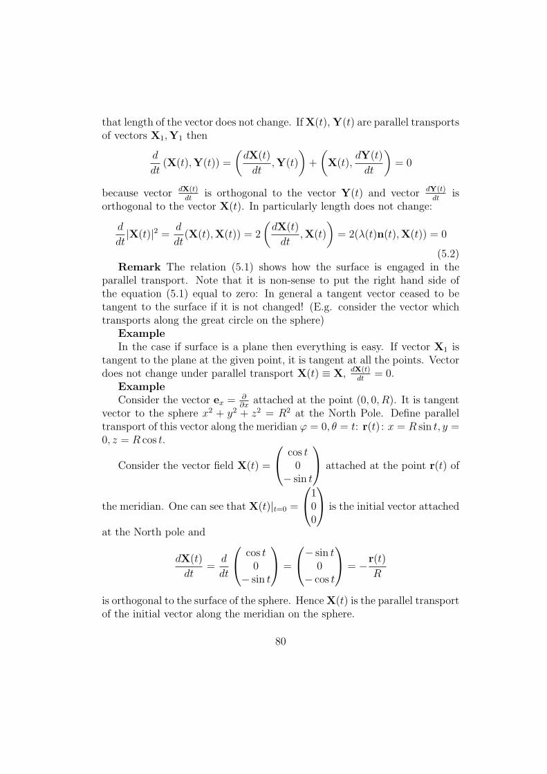
that length of the vector does not change. IfX(t),Y(t) are parallel transportsof vectors X1,Y1 then

d

dt(X(t),Y(t)) =

(dX(t)

dt,Y(t)

)+

(X(t),

dY(t)

dt

)= 0

because vector dX(t)dt

is orthogonal to the vector Y(t) and vector dY(t)dt

isorthogonal to the vector X(t). In particularly length does not change:

d

dt|X(t)|2 = d

dt(X(t),X(t)) = 2

(dX(t)

dt,X(t)

)= 2(λ(t)n(t),X(t)) = 0

(5.2)Remark The relation (5.1) shows how the surface is engaged in the

parallel transport. Note that it is non-sense to put the right hand side ofthe equation (5.1) equal to zero: In general a tangent vector ceased to betangent to the surface if it is not changed! (E.g. consider the vector whichtransports along the great circle on the sphere)

ExampleIn the case if surface is a plane then everything is easy. If vector X1 is

tangent to the plane at the given point, it is tangent at all the points. Vectordoes not change under parallel transport X(t) ≡ X, dX(t)

dt= 0.

ExampleConsider the vector ex = ∂

∂xattached at the point (0, 0, R). It is tangent

vector to the sphere x2 + y2 + z2 = R2 at the North Pole. Define paralleltransport of this vector along the meridian φ = 0, θ = t: r(t) : x = R sin t, y =0, z = R cos t.

Consider the vector field X(t) =

cos t0

− sin t

attached at the point r(t) of

the meridian. One can see that X(t)|t=0 =

100

is the initial vector attached

at the North pole and

dX(t)

dt=

d

dt

cos t0

− sin t

=

− sin t0

− cos t

= −r(t)

R

is orthogonal to the surface of the sphere. HenceX(t) is the parallel transportof the initial vector along the meridian on the sphere.

80

We consider other more sophisticated examples of parallel transport of vectors along

curves on surfaces in Appendices.

5.2 Geometrical meaning of Gaussian curvature. The-orema Egregium

We know that Gaussian curvature of cylinder cone and plane equals to zeroand Gaussian curvature of sphere equals to 1

R2 (see the calculations in theend of the subsection 4.7 and Homework 8.)

We know that we can form cylindrical surface and cone surface bendingthe sheet of paper without ”shrinking”. On the other hand one can not forma part of sphere from the sheet of the paper without ”shrinking” it. How toexpress mathematically this fact?

Consider on the sheet of the paper two close points A,B and the segmentAB. The length of this segment is the shortest distance between points Aand B. Any curve starting at the point A and finishing at the point B has thelength which is greater or equal than the length of the segment AB. When weform cylindrical (or conic) surface bending the sheet of the paper we do notdistort this property. The segment AB on the cylindrical surface will becomethe curve which we will denote also AB, but the length of this curve will bethe same and it will be the shortest curve amongst all the curves connectingthe points A and B. Internal observer (”ant” mathematician living on thecylindrical surface) observes that the curve AB on the cylinder has the samelength as it has before (being the segment on flat sheet of the paper). This isstrictly related with the fact that Gaussian curvature of the cylinder surfaceequals to zero.

Theorem (Theorema Eggregium) The Gaussian curvature of surface isdefined by first quadratic form. If Two surfaces have the same quadratic formthen they have the same Gaussian curvature.

In other words if we measure the length of the curves and angles betweenthem on two surfaces we will come to the same answers, then these surfaceshave the same Gaussian curvature.

In particular if a surfaces have vanishing Gaussian curvature then locallyone comes to this surface bending the sheet of the paper without ”shrinking”.

This Theorem explains why sphere even locally cannot be transformed tothe plane without distorting.

This remarkable Theorem which belongs to Gauss is the foundation result

81

in differential geometry.The proof of Theorem will be given in the course of Riemannian geometry.Note that we calculated Gaussian curvature using Shape operator, i.e. in terms of

External observer. The Theorem says that Gaussian curvature depends only on distanceson the surface, hence the internal observer can calculate the gaussian curvature. How itcan be done?

We will formulate another Theorem which is strictly related with the TheoremaEgregium and explains how internal observer can calculate Gaussian curvature.

Theorem Let C be a closed curve on a surface M such that C is a boundary of acompact oriented domain D ⊂ M , then during the parallel transport of an arbitrary tangentvector along the closed curve C the vector rotates through the angle

∆Φ = ∠ (X,RCX) =

∫D

Kdσ , (5.3)

where K is the Gaussian curvature and dσ =√det gdudv is the area element induced by

the First quadratic form on the surface on the surface M , i.e. dσ =√det gdudv.

In particular if Gaussian curvature K is constant then

∆Φ = ∠ (X,RCX) = KS (5.4)

For example consider the sphere x2 + y2 + z2 = R2 and the triangle ABC on it withvertices A = (0, 0, 1), B = (1, 0, 0) and C = (cosφ, sinφ, 0). Then during parallel transportof the vector along the triangle ABC it will rotate on the angle φ (see the Homework 8).On the other hand the area of this triangle equals to S = R2φ. We see that

φ =S

R2= KS

The angle of rotation of tangent vector in fact depends only on the internal geometryof surface. Thus the relation above can be used for proving the Theorema Egregium.

The Theorem above has very interestingCorollary Let ABC be triangle on the surface M where AB,AC,BC are shortest

curves connecting the points A,B,C. Let α, β, γ be angles of this triangle. For usualtriangle sum of angles equal to π. It turns out that for triangel on the surface the sum ofangles is related with Gaussian curvature:

α+ β + γ − π =

∫ABC

Kdσ (5.5)

Internal observer may use this formula for calculating gaussian curvature at any givenpoint: He draws the triangle calculate the sum of angles and see that

K ≈ α+ β + γ − π

S

(See in more detail ”A tale on differential geometry” in Appendices.)

82

6 †Appendices

6.1 Formulae for vector fields and differentials in cylin-drical and spherical coordinates

Cylindrical and spherical coordinates

• Cylindrical coordinates in E3x = r cosφ

y = r sinφ

z = h

(0 ≤ φ < 2π, 0 ≤ r < ∞) (6.1)

• Spherical coordinates in E3x = r sin θ cosφ

y = r sin θ cosφ

z = r cos θ

(0 ≤ φ < 2π, 0 ≤ r < ∞)−−− cylindrical coordiantes in E3

(6.2)

Example (Basis vectors and forms for cylindrical coordinates)Consider cylindrical coordinates in E3: u = r, v = φ,w = h. Then calculating partial

derivatives we come to

∂r = ∂x∂r ∂x + ∂y

∂r ∂y +∂z∂r∂z = cosφ∂x + sinφ∂y

∂φ = ∂x∂φ∂x + ∂y

∂φ∂y +∂z∂φ∂z = −r sinφ∂x + r cosφ∂y

∂h = ∂x∂h∂x + ∂y

∂h∂y +∂z∂h∂z = ∂z

(6.3)

Basic forms are dr, dφ, dh and

dr(∂r) = 1, dr(∂φ) = 0, dr(∂h) = 0

dφ(∂r) = 0, dφ(∂φ) = 1, dφ(∂h) = 0

dh(∂r) = 0, dh(∂φ) = 0, dh(∂h) = 1

(6.4)

Example (Basis vectors for spheric coordinates)Consider spheric coordinates in E3: u = r, v = θ, w = φ. Then calculating partial

derivatives we come to

∂r = ∂x∂r ∂x + ∂y

∂r ∂y +∂z∂r∂z = sin θ cosφ∂x + sin θ sinφ∂y + cos θ∂z

∂θ = ∂x∂θ ∂x + ∂y

∂θ∂y +∂z∂θ∂z = r cos θ cosφ∂x + r cos θ sinφ∂y − r sin θ∂z

∂φ = ∂x∂φ∂x + ∂y

∂φ∂y +∂z∂φ∂z = −r cos θ sinφ∂x + r sin θ cosφ∂y

(6.5)

83

Basic forms are dr, dθ, dφ and

dr(∂r) = 1, dr(∂θ) = 0, dr(∂φ) = 0

dθ(∂r) = 0, dθ(∂θ) = 1, dθ(∂φ) = 0

dφ(∂r) = 0, dφ(∂θ) = 0, dφ(∂φ) = 1

(6.6)

We know that 1-form is a linear function on tangent vectors. If A,B are two vectorsattached at the point r0, i.e. tangent to this point and ω, ρ are two 1-forms then onedefines the value of ω ∧ ρ on A, B by the formula

ω ∧ ρ(A,B) = ω(A)ρ(B)− ω(B)ρ(A) (6.7)

We come to bilinear anisymmetric function on tangent vectors. If σ = a(x, y)dx ∧ dyis an arbitrary two form then this form defines bilinear form on pair of tangent vectors:σ(A,B) =

a(x, y)dx ∧ dy(A,B) = a(x, y) (dx(A)dy(B)− dx(B)dy(A)) = a(x, y)(AxBy −AyBy)(6.8)

One can see that in the case if a = 1 then right hand side of this formula is nothing butthe area of parallelogram spanned by the vectors A,B.

This leads to the conception of integral of form over domain.Let ω = a(x)dx ∧ dy be a two form and D be a domain in E2. Then by definition∫

D

ω =

∫D

a(x, y)dxdy (6.9)

If ω = dx ∧ dy then ∫D

w =

∫D

(x, y)dxdy = Area of the domain D (6.10)

The advantage of these formulae is that we do not care about coordinates9

Example Let D be a domain defined by the conditionsx2 + y2 ≤ 1

y ≥ 0(6.12)

Calculate∫Ddx ∧ dy.

9If we consider changing of coordinates then jacobian appears: If u, v are new coordi-nates, x = x(u, v), y = y(u, v) are new coordinates then∫

a(x, y)dxdy =

∫a(x(u, v), y(u, v)) det

(xu xv

xu xv

)dudv (6.11)

In formula(6.9) it appears under as a part of coefficient of differential form.

84

∫Ddx ∧ dy =

∫Ddxdy = area of the D = π

2 .If we consider polar coordinates then according (2.44)

dx ∧ dy = rdr ∧ dφ

Hence∫Ddx ∧ dy =

∫Drdr ∧ dφ =

∫Drdrdφ =

∫ 1

0

(∫ π

0dφ)rdr = π

∫ 1

0rdr = π/2.

Another exampleExample Let D be a domain in E2 defined by the conditions

(x−c)2

a2 + y2

b2 ≤ 1

y ≥ 0(6.13)

D is domain restricted by upper half of the ellipse and x-axis. Ellipse has the centreat the point (c, 0). Its area is equal to S =

∫Ddx ∧ dy. Consider new variables x′, y′:

x = c + ax′, y = by′. In new variables domain D becomes the domain from the previousexample:

(x− c)2

a2+

y2

b2= x′2 + y′

2

and dx ∧ dy = abdx′ ∧ dy′. Hence

S =

∫(x−c)2

a2 + y2

b2≤1,y≥0

dx ∧ dy = ab

∫x′2+y′2≤1,y′≥0

dx′ ∧ dy′ =πab

2(6.14)

Theorem 2 ( Green formula) Let ω be 2-form such that ω = dω′ and D be a domain–interior of the closed curve C. Then ∫

D

w =

∫C

w′ (6.15)

6.2 Curvature and second order contact (touching) ofcurves

Let C1, C2 be two curves in E2. For simplicity we here consider only curves in E2.

Definition Two non-parameterised curves C1, C2 have second order contact (touch-ing) at the point r0 if

• They coincide at the point r0

• they have the same tangent line at this point

• they have the same curvature at the point r0

If r1(t), r2(t) are an arbitrary parameterisations of these curves such that r1(t0) =r2(t0) = r0 then the condition that they have the same tangent line means that velocityvectors v1(t),v2(t) are collinear at the point t0.

85

(As always we assume that curves under considerations are smooth and regular, i.e.x(t), y(t) are smooth functions and velocity vector v(t) = 0.)

Example Consider two curves Cf , Cg—graphs of the functions f1, f2. Recall thatcurvature of the graph of the function f at the point (x, y = f(x)) is equal to (see (3.29))

k(x) =f ′′(x)

(1 + f ′(x))32

(6.16)

Then condition of the second order touching at the point r0 = (x0, y0) means thatThey coincide at the point r0: f(x0) = g(x0)

They have the same tangent line at this point: f ′(x0) = g′(x0)

They have the same curvature at the point r0:f ′′(x0)

(1+f ′(x0))32= g′′(x0)

(1+g′(x0))32, i.e. f ′′(x0) = g′′(x0)

We see that second order touching means that difference of the functions in vicinity of thepoint x0 is of order o((x− x0)

2). Indeed due to Taylor formula

f(x) = f(x0) + f ′(x0)(x− x0) +12f

′′(x0)(x− x0)2 + . . .

g(x) = g(x0) + g′(x0)(x− x0) +12g

′′(x0)(x− x0)2 + . . .

(6.17)

where we denote by dots terms which are o(x − x0)2. (They say that f(x) = o(x − x0)

n

if limx→x0

f(x)(x−x0)n

= 0).

Hencef(x)− g(x) = o(x− x0)

2 (6.18)

because f(x0) = g(x0), f(x0) = g(x0), f′(x0) = g′(x0) and f ′′(x0) = g′′(x0)

In general case if two curves have second order contact then in the vicinity of thecontact point one can consider these curves as a graphs of the functions y = f(x) (orx = f(y)).

To clarify geometrical meaning of second order touching consider the case where oneof the curves is a circle. Then second order touching means that curvature of one of thesecurves is equal to 1/R, where R is a radius of the circle.

We see that to calculate the radius of the circle which has the second order touchingwith the given curve at the given point we have to calculate the curvature of this curve atthis given point.

Example. Let C1 be parabola y = ax2 and C2 be a circle. Suppose these curves havesecond order contact at the vertex of the parabola: point 0, 0.

Calculate the curvature of the parabola at the vertex. Curvature at the vertex is equalto k(t)|t=0 = 2a (see Homework). Hence the radius of the circle which has second ordertouching is equal to

R =1

2a.

To find equation of this circle note that the circle which has second order touching toparabola at the vertex passes trough the vertex (point (0, 0)) and is tangent to x-axis.

86

The radius of this circle is equal to R = 12a . Hence equation of the circle is

(x−R2) + y2 = 0, where R =1

2a

One comes to the same answer by the following detailed analysis:Consider equation of a circle: (x− x0)

2 + (y − y0)2 = R2. The condition that curves

coincide at the point (0, 0) means that x20 + y20 = R2. x-axis is tangent to parabola at

the vertex. Hence it is tangent to the circle too. Hence y20 = R2 and x0 = 0. Wesee that an equation of the circle is x2 + (y − R)2 = R2. The circle x2 + (y − R)2 =x2 + y2 − 2yR = 0 in the vicinity of the point (0, 0) can be considered as a graph of thefunction y = R−

√R2 − x2 .. The condition that functions y = ax2 and y = R−

√R2 − x2

have second order contact means that

R−√R2 − x2 = ax2 + terms of the order less that x2 .

But

R−√R2 − x2 = R−R

√1− x2

2R2= R−R

(1− x2

2R2+ o(x2)

)=

x2

2R+ o(x2) .

Comparing we see that a = 12R and 1

R = 2a. But curvature of the parabola at the vertexis equal to k = 2a (if a > 0). We see that k = 1

R .

6.3 Integral of curvature over planar curve.

We consider here the following problem: Let C = r(t) be a planar curve, i.e. a curve inE2.

Let n(r(t) be a unit normal vector field to the curve, i.e. n is orthogonal to the curve(velocity vector) and it has unit length.

E.g. if r(t) : x(t) = R cos t, y(t) = R sin t, then n(r(t)) =

(cos tsin t

)If point moves along the curve r(t), t1 ≤ t ≤ t2 then velocity vector and vector field

n(t) rotate on the same angle. It turns out that this angle is expressed via integral ofcurvature over the curve...

Try to analyze the situation:

Proposition Let C : r(t) be a curve in E2, v(t) = dr(t)dt , velocity vector, k(r(t))—

curvature and n(t) unit normal vector field. Denote by φ(t) the angle between normalvector n(t) and x-axis.

Thendn(t)

dt= ±k(r(t))v(t) (6.19)

dφ(t)

dt= ±k(r(t))|v(t)| (6.20)

(Sign depends on the orientation of the pair of vectors (v,n))

87

Note that the second statement of the Proposition has a clear geometrical meaning:If C is a circle of the radius R then RHS of (6.20) is equal to v

R . It is just angular velocitydφ/dt.

To prove this Proposition note that (n,n) = 1. Hence

0 =d

dt(n(t),n(t)) = 2

(dn(t)

dt,n(t)

),

i.e. vector dn(t)dt is orthogonal to the vector n. This means that dn(t)

dt is collinear to v(t),

because curve is planar. We have dn(t)dt = κ(r(t))v(t) where κ is a coefficient. Show that

the coefficient κ is just equal to curvature k (up to a sign). Clearly (n,v) = 0 becausethese vectors are orthogonal. Hence

0 =d

dt(n(t),v(t)) =

(dn(t)

dt,v(t)

)+

(n(t),

dv(t)

dt

)=

(κ(r(t))v(t),v(t)) + (n(t),a(t)) = κ(r(t))|v(t)|2 + (n,a⊥) ,

because (n(t),a(t)) = (n,a⊥). But (n,a⊥) is just centripetal acceleration: (n,a⊥) =

±|a⊥| and curvature is equal to |a⊥|/|v|2. Hence we come to κ(r(t)) = ± |a⊥||v|2 = ±k. Thus

we prove (6.19).To prove (6.20) consider expansion of vectors n(t),v(t) over basis vectors ∂x, ∂y. We

see that

n(t) = cosφ(t)∂x + sinφ(t)∂y and v(t) = |v(t)| (− sinφ(t)∂x + cosφ(t)∂y) (6.21)

Differentiating n(t) by t we come to dn(t)dt = dφ(t)

dt (− sinφ(t)∂x + cosφ(t)∂y) =dφ(t)dt

v(t)|v(t)| .

Comparing this equation with equation (6.19) we come to (6.20).The appearance of sign factor in previous formulae related with the fact that normal

vector field is defined up to a sign factor n → −n.It is useful to write formulae (6.19), (6.20) in explicit way. Let r(t) : x(t), y(t) be a

parameterisation of the curve. Then v(t) =

(xt

yt

)velocity vector. One can define normal

vector field as

n(t) =1√

x2t + y2t

(−ytxt

)(6.22)

or changing the sign as

n(t) =1√

x2t + y2t

(yt−xt

)(6.23)

If we consider (6.22) for normal vector field then

dn(t)

dt=

xttyt − yttxt

(x2t + y2t )

32

(xt

yt

)(6.24)

88

Recalling that k =|xttyt−ytt|xt

(x2t+y2

t )32

we come to (6.19). For the angle we have

dφ

dt=

xtytt − ytxtt

(x2t + y2t )

32

√x2t + y2t =

xtytt − ytxtt

(x2t + y2t )

(6.25)

This follows from the considerations above but it can be also calculated straightforwardly.Remark Note that last two formulae do not possess indefenity in sign.

This Proposition has very important application. Consider just two examples:Consider upper half part of the ellipse x2/a2 + y2/b2 = 1, y ≥ 0. We already know

that curvature at the point x = a cos t, y = b cos t of the ellipse is equal to

k =ab

(a2 sin t2t+ b2 cos2 t)3/2

and speed is equal to√

a2 sin2 t+ b2 cos2 t Apply formula (6.20) of Proposition. Thecurvature is not equal to zero at all the point. Hence the sign in the (6.20) is the same forall the points, i.e.

π =

∫ π

0

dφ(t)dt = ±∫ π

0

k(r(t))|v(t)| = (6.26)∫ π

0

ab

(a2 sin2 t+ b2 cos2 t)3/2

√a2 sin2 t+ b2 cos2 t dt =

∫ π

0

abdt

a2 sin2 t+ b2 cos2 t.

We calculated this integral using geometrical considerations: left hand side represents theangle of rotation of normal unit vector and this angle is equal to π. Try to calculate thelast integral straightforwardly: it is not easy exercise in calculus.

Another example: Let r = r(t), x = x(t), y = y(t), t1 ≤ t ≤ t2 be a closed curve inE2 (r(t1) = r(t2).) We suppose that it possesses self-intersections points. We cannot usa formula (6.20) for integration because in general curvature may vanish at some points,but we still can use the formula (6.25). The rotation of the angle φ is equal to 2πn, (n-iscalled winding number of the curve). Hence according to (6.25) see that∫ t2

t1

xtytt − xtyttx2t + y2t

= 2πn

or1

2π

∫ t2

t1

xtytt − xtyttx2t + y2t

= n (6.27)

The integrand us equal to the curvature multiplied by the speed (up to a sign). Left hand

side is integral of continuous function divided by transcendent number π. The geometry

tells us that the answer must to be equal to integer number.

89

6.4 Relations between usual curvature normal curva-ture and geodesic curvature.

Consider at any point p of the curve the following basis v, f , n, where• velocity vector v is tangent to the curve

• the vector f is the vector tangent to the surface but orthogonal to the vector v.

• n is the unit normal vector to the surface, i.e.it is orthogonal to vectors v and f .

Decompose acceleration vector over three directions, i.e. over three one-dimensionalspaces spanned by vectors v, f and n:

a = aorthogonal to surface + atang.to surf. and orthog. to curve + atangent to curve(6.28)

The vector aorthogonal to surface which is collinear to normal unit vector n, will be

called vector of normal acceleration of the curve on the surface. We denote it by an.The vector atang.to surf. and orthog. to curve , collinear to unit vector fC will be

called vector of geodesic acceleration . We denote it by ageod.The vector atangent to curve , collinear to velocity vector v, is just vector of tangential

acceleration . We denote it atang. We can rewrite (6.28) as

a = an + ageod + atang (6.29)

Study the expansion (6.29). Both vectors an and ageod are orthogonal to the curve.The vector ageod is orthogonal to the curve but it is tangent to the surface. The vectoran is orthogonal not only to the curve. It is orthogonal to the surface.

The vector ageod + an = a⊥ is orthogonal to the curve. It is the vector of normalacceleration of the curve.

Remark Please note that when we consider the curves on the surface it could arisethe confusion between the vector an—normal acceleration of the curve on the surface andthe vector a⊥ of normal acceleration of the curve (see (3.2)).

When we decompose in (6.29) the acceleration vector a in the sum of three vectorsan,ageod and atang then the vector an, the normal acceleration of the curve on the surfaceis orthogonal to the surface not only to the curve. The vector

a⊥ = an + ageod,

is orthogonal only to the curve and in general it is not orthogonal to the surface (ifageod = 0). It is the normal acceleration of the curve. It depends only on the curve.The normal acceleration an of the curve on the surface which is orthogonal to the surfacedepends on the surface where the curve lies.

We know that the curvature of the curve is equal to the magnitude of normal acceler-ation of the curve divided on the square of the speed (see (3.22)). We have:

curvature of the curve k =|a⊥||v|2

=|an + ageod|

|v|2.

90

The vectors an and ageod transform under reparameterisation in the same way as a vectora⊥ (see (3.11)). If t → t(τ) then

a′⊥(τ) = t2τa⊥ and a′n(τ) = t2τan(t), a′geod(τ) = t2τageod(t) (6.30)

where a′(τ) = d2

dτ2 r(t(τ)) = t2τa+ tττv (see (3.9), (3.10), (3.8)). Hence the magnitudes

|ageod||v|2

and|an||v|2

(6.31)

are reparameterisation invariant as well as magnitude k = |a⊥||v|2 =

|an+ageod||v|2 .

Multiply left and right hand sides of the equation (6.29) on unit normal vector n.Then (atang,n) = (ageod,n) = 0 because vectors ageod and atang are orthogonal to thevector n. We come to the relation

an = (n,a)n and , |an| = |(a,n)| . (6.32)

Or in other words scalar product (n,a) is equal to |an| (up to a sign).Compare the formula

κn =(n,a)

(v,v)(6.33)

(see (4.27)) for normal curvature with the formula

k =|a⊥|(v,v)

for usual curvature (see (3.22)).It follows from (6.30), (6.31) and (4.27) (or (6.33)) that for any curve on the surface

the modulus of the normal curvature is less or equal than usual curvature.

|κn| ≤ k (6.34)

Indeed we have for usual curvature

k =|a⊥||v|2

=|ageod + anormal|

|v|2=

√a2geod + a2norm

|v|2≥ |anormal|

|v|2= |κn| (6.35)

Normal curvature is a positive or negative real number. (Usual curvature is non-negative real number). Normal curvature changes a sign if n → −n.

Remark We obtained in (6.31) that the magnitude|ageod||v|2 is reparameterisation in-

variant. It defines so called geodesic curvature κgeod =|ageod||v|2 . We see that usual curvature

k, normal curvature κ and geodesic curvature κgeod are related by the formula

k2 = κ2geod + κ2

normal (6.36)

91

6.5 Normal curvature of curves on cylinder surface.

Example Consider an arbitrary curve C : h = h(t), φ = φ(t) on the cylinder

r(φ, h) :

x = R cosφ

y = R sinφ

z = h

Pick any point p on this curve and find normal acceleration vector at this point of thiscurve.

Without loss of generality suppose that point p is just a point (R, 0, 0). Note thatvector ex attached at the point (R, 0, 0) is unit vector orthogonal to the surface of cylinder,i.e. ex = −n at the point p = (R, 0, 0).

RemarkUnit vector, as well as normal curvature is defined up to a sign. It is conve-nient for us to choose n = −ex, not n = ex.

Vectors ey, ez are tangent to the surface of cylinder. At the point p = (R, 0, 0)φ = 0, h = 0.

We have

v =dr(t)

dt=

dx(t)

dtex +

dy(t)

dtey +

dz(t)

dtez =

Rd cosφ(t)

dtex +R

d sinφ(t)

dtey +

dh(t)

dtez = −R sinφφex +R cosφφey + hez

Thus v = Rφey + hez at the point p = (R, 0, 0) . (6.37)

For acceleration vector

a =d2r(t)

dt2=

d2x(t)

dt2ex+

d2y(t)

dt2ey+

d2z(t)

dt2ez = R

d2 cosφ(t)

dt2ex+R

d2 sinφ(t)

dt2ey+

d2h(t)

dt2ez =

R(−(φ)2 cosφ− ..

φ sinφ)ex+R

(−(φ)2 sinφ+

..φ cosφ

)ey+

..

hez =..φRey+

..

hez − (φ)2Rex

at the point p = (R, 0, 0) where cosφ = 0, sinφ = 1. We see that

a =..φRey +

..

hez︸ ︷︷ ︸tangent to the surface

− (φ)2Rex︸ ︷︷ ︸normal to the surface

(6.38)

We see that an = (φ)2Rex. Comparing with velocity vector (6.37) we see that

an =v2horizontal

Rn (6.39)

We see that for any curve on the cylinder x2 + y2 = R2 the normal curvature (an,n)|v|2

(see (4.27)) is equal to(an,n)

|v|2=

Rφ2

R2φ2 + h2(6.40)

92

and it obeys relations

0 ≤ κnormal ≤1

R

depending of the curve. E.g. if the curve on the cylinder is a straight line x = x0, y =y0, z = t then a = 0 and normal curvature of this curve is equal to the naught as well asusual curvature.

If the curve is circle x = R cos t, y = R sin t, z = z0 then normal curvature of this curveas well as usual curvature is equal to 1

R .

Remark Very important conclusion from this example is

normal curvature of the cylinder of the radius R takes values in the interval(0, 1

R

). It

cannot be greater than 1R

Note that we can consider on cylinder very curly curve of very big curvature. The normalcurvature at the points of this curve will be still less than 1

R .

At any point of the surface normal curvature in general depends on the curve but ittakes values in the restricted interval.

E.g. for the sphere of radius R one can see that normal curvature at any point isequal to 1

R independent of curve. In spite of this fact the usual curvature of curve can bevery big 10. If we consider the circle of very small radius r on the sphere then its usualcurvature is equal to k = 1

r and k → ∞ if r → 0 So we see that one can define curvatureof surface in terms of normal curvature.

6.6 Parallel transport of vectors tangent to the sphere.

1. Consider now in a more detail the parallel transport along curves on sphere.In the case if surface is a plane then everything is easy. If vector X1 is tangent to

the plane at the given point, it is tangent at all the points. Vector does not change underparallel transport X(t) ≡ X.

Consider a case of parallel transport along curves on the sphere.

Consider on the sphere x2 + y2 + z2 = a2 (a is a radius) tangent vectors:

rθ =

a cos θ cosφa cos θ sinφ−a sin θ

rφ =

−a sin θ sinφa sin θ cosφ

0

(6.41)

attached at the point r(θ, φ) =

a sin θ cosφa sin θ sinφ

a cos θ

. One can see that

(rθ, rθ) = a, (rh, rφ) = 0, (rφ, rφ) = a2 sin2 θ

10It is the geodesic curvature of the curves which characterises its curvature with respectto the curve. The relation between usual geodesic and normal curvature is given by theformula (6.36).

93

It is convenient to introduce vectors which are parallel to these vectors but have unitlength:

eθ =rθa, eφ =

rφa sin θ

(eθ, eθ) = 1, (eθ, eφ) = 0, (eφ, eφ) = 1 . (6.42)

How these vectors change if we move along parallel (i.e. what is the value of ∂eθ

∂φ ,∂eφ

∂φ );

how these vectors change if we move along meridians (i.e. what is the value of ∂eθ

∂θ ,∂eφ

∂θ ).

First of all recall that unit normal vector to the sphere at the point θ, φ is equal to r(θ,φ)a :

n(θ, φ) =

sin θ cosφsin θ sinφ

cos θ

Now calculate:

∂eθ∂θ

=∂

∂θ

cos θ cosφcos θ sinφ− sin θ

=

− sin θ cosφ− sin θ sinφ

− cos θ

= −n (6.43)

,

∂eθ∂φ

=∂

∂φ

cos θ cosφcos θ sinφ− sin θ

=

− cos θ sinφcos θ cosφ

0

= cos θeφ, (6.44)

,

∂eφ∂θ

=∂

∂θ

− sinφcosφ0

=

− cos θ sinφcos θ cosφ

0

= 0, (6.45)

∂eφ∂φ

=∂

∂φ

− sinφcosφ0

=

− cosφ− sinφ

0

= − sin θn− cos θeθ, (6.46)

Some of these formulaes are intuitively evident: For example formula (6.43) whichmeans that family of the vectors eθ(θ) is just parallel transport along meridian, becauseits derivation is equal to −n.

Another intuitively evident example: consider the meridian θ(t) = t, φ(t) = φ0,0 ≤ t ≤ π. It is easy to see that the vector field

X(t) = eθ(θ(t), φ0) =

cos θ(t) cosφ0

cos θ(t) sinφ0

− sin θ(t)

attached at the point (θ(t), φ0) is a parallel transport because for family of vectors X(t)all the conditions of parallel transport are satisfied. In particular according to (6.43)

dX(t)

dt=

dθ(t)

dt

∂

∂θ

cos θ cosφcos θ sinφ− sin θ

= −n(θ(t), φ0)

Now consider an example which is intuitively not-evident.

94

Example. Calculate parallel transport of the vector eφ along the parallel. On thesphere of the radius a consider the parallel

θ(t) = θ0, φ(t) = t, 0 ≤ t ≤ 2π (6.47)

In cartesian coordinates equation of parallel will be:

r(t) =

a sin θ(t) cosφ(t)a sin θ(t) sinφ(t)

−a cos θ(t)

=

a sin θ0 cos ta sin θ(t) sin t−a cos θ0

, 0 ≤ t ≤ 2π (6.48)

It is easy to see that the family of the vectors eφ(θ0, φ(t)) on parallel, is not parallel

transport! becausedeφ(θ0,φ(t))

dt =deφ(θ0,φ)

dφ is not equal to zero (see (6.46) above). Let a

family of vectors X(t) be a parallel transport of the vector eφ along the parallel (6.47):X(t) = a(t)eθ(t)+b(t)eφ(t) where a(t), b(t) are components of the tangent vectorX(t) withrespect to the basis eθ, eφ at the point θ = θ0, φ = t on the sphere. Initial conditions forcoefficients are a(t)|t=0 = 0, b(t)|t=0 = 1 According to the definition of parallel transportand formulae (6.43)—(6.46) we have:

dX(t)

dt=

d (a(t)eθ(t) + b(t)eφ(t))

dt=

(da(t)

dt

)eθ + a(t) cos θ0eφ +

db(t)

dteφ+

b(t) (− sin θ0n− cos θeθ) =

=

(da(t)

dt− b(t) cos θ0

)eθ +

(db(t)

dt+ a(t) cos θ0

)eφ − b(t) sin θ0n (6.49)

Under parallel transport only orthogonal component of the vector changes. Hence wecome to differential equations

da(t)dt − wb(t) = 0

db(t)dt + wa(t)

a(0) = 0, b(0) = 0, w = cos θ0 (6.50)

The solution of these equations is a(t) = sinwt, b(t) = coswt. We come to the followinganswer: parallel transport along parallel θ = θ0 of the initial vector eφ is the family

X(t) = sinwt eθ + coswt eφ, w = cos θ0 (6.51)

During traveling along the parallel θ = θ0 the eθ component becomes non-zero At theend of the traveling the initial vector X(t)|t=0 = eφ becomes X(t)|t=2π = sin 2πweθ +cos 2πweφ: the vector eφ after woldtrip traveling along the parallel θ = θ0 trans-forms to the vector sin(2π cos θ0)eθ + cos(2π cos θ0)eφ. In particularly this meansthat the vector eφ after parallel transport will rotate on the angle

angle of rotation = 2π cos θ0

Compare the angle of rotation with the area of the segment of the sphere above theparallel θ = θ0. According to the formula (??) area of this segment is equal to S =2πah = 2πa2(1 − cos θ0). On the other hand Gaussian curvature of the sphere is equalto 1

a2 . Hence we see that up to the sign angle of rotation is equal to area of the seqmentdivided on the Gaussian curvature:

∆φ = ± S

K= ±2π cos θ0 (6.52)

95

6.7 Parallel transport along a closed curve on arbi-trary surface.

The formula above for the parallel transport along parallel on the sphere keeps in thegeneral case.

Theorem Let M be a surface in E3. Let r(t) : r(t), t1 ≤ t ≤ t2, r(t1) = r(t2) be aclosed curve on the surface M such that it is a boundary of domain D of the surface M .(We suppose that the domain D is bounded an orientate.) Let X(t) be a parallel transportof the arbitrary tangent vector along this closed curve. Consider initial and final vectorsX(t1),X(t2). They have the same length according to (5.2).

Theorem The angle ∆φ between these vectors is equal to the integral of Gaussiancurvature over the domain D:

∆φ = ±∫D

Kdσ (6.53)

where we denote by dσ the element of the area of surface of M .

The calculations above for traveling along the parallel are just example of this Theo-rem. The integral of Gaussian curvature over the domain above parallel θ = θ0 is equalto K · 2πa(1− cos θ0)=

1a2 · 2πa2(1− cos θ0) = 2π(1− cos θ0). This is equal to the angle of

rotation 2π cos θ0 (up to a sign and modulo 2π). Another simpleExample. Consider on the sphere x2+ y2+ z2 = a2 points A = (0, 0, 1), B = (1, 0, 0)

and C = (0, 1, 0). Consider arcs of great circles which connect these points. Consider thevector ex attached at the point A. This vector is tangent to the sphere. It is easy to seethat under parallel transport along the arc AB it will transform at the point B to thevector −ez. The vector −ez under parallel transport along the arc BC will remain thesame vector −ez. And finally under parallel transport along the arc CA the vector −ezwill transform at the point A to the vector −ey. We see that under traveling along thecurvilinear triangle ABC vector ex becomes the vector −ey, i.e. it rotates on the angle π

2 .

It is just the integral of the curvature 1a2 over the triangle ABC: K · S = 1

a2 · 4πa2

8 = π2 .

We know that for planar triangles sum of the angles is equal to π. It turns out thatCorollary Let ABC be a triangle on the surface formed by geodesics. Then

∠A+ ∠B + ∠C = π +

∫ABC

Kds (6.54)

The Gaussian curvature measures the difference of π and sum of angles.The corollary evidently follows form the Theorem. It is of great importance: It gives

us tool to measure curvature. (See the tale about ant.)

6.8 Gauss Bonnet Theorem

Consider the integral of curvature over whole closed surface M . According to the Theoremabove the answer has to be equal to 0 (modulo 2π), i.e. 2πN where N is an integer, becausethis integral is a limit when we consider very small curve. We come to the formula:∫

D

Kdσ = 2πN

96

(Compare this formula with formula (6.27)).What is the value of integer N?We present now one remarkable Theorem which answers this question and prove this

Theorem using the formula (6.54).Let M be a closed orientable surface.11 All these surfaces can be classified up to a dif-

feomorphism. Namely arbitrary closed oriented surfaceM is diffeomorphic either to sphere(zero holes), or torus (one hole), or pretzel (two holes),... ”Number k” of holes is intuitivelyevident characteristic of the surface. It is related with very important characteristic—Eulercharacteristic χ(M) by the following formula:

χ(M) = 2(1− g(M)), where g is number of holes (6.55)

RemarkWhat we have called here ”holes” in a surface is often referred to as ”handles”attached o the sphere, so that the sphere itself does not have any handles, the torus hasone handle, the pretzel has two handles and so on. The number of handles is also calledgenus.

Euler characteristic appears in many different way. The simplest appearance is thefollowing:

Consider on the surface M an arbitrary set of points (vertices) connected with edges(graph on the surface) such that surface is divided on polygons with (curvilinear sides)—plaquets. (”Map of world”)

Denote by P number of plaquets (countries of the map)Denote by E number of edges (boundaries between countries)Denote by V number of vertices.Then it turns out that

P − E + V = χ(M) (6.56)

It does not depend on the graph, it depends only on how much holes has surface.E.g. for every graph on M , P −E + V = 2 if M is diffeomorphic to sphere. For every

graph on M P − E + V = 0 if M is diffeomorphic to torus.

Now we formulate Gauß -Bonnet Theorem.Let M be closed oriented surface in E3.Let K(p) be Gaussian curvature at any point p of this surface.Recall that sign of Gaussian curvature does not depend on the orientation. If we

change direction of normal vector n → −n then both principal curvatures change the signand Gaussian curvature K = detA/detG does not change the sign 12.

11Closed means compact surface without boundaries. Intuitively orientability meansthat one can define out and inner side of the surface. In terms of normal vectors ori-entability means that one can define the continuous field of normal vectors at all thepoints of M . The direction of normal vectors at any point defines outward direction.Orientable surface is called oriented if the direction of normal vector is chosen.

12For an arbitrary point p of the surface M one can always choose cartesian coordinates(x, y, z) such that surface in a vicinity of this spoint is defined by the equation z =ax2 + bx2 + . . . , where dots means terms of the order higher than 2. Then Gaussian

97

Theorem (Gauß -Bonnet) The integral of Gaussian curvature over the closed compactoriented surface M is equal to 2π multiplied by the Euler characteristic of the surface M

1

2π

∫M

Kdσ = χ(M) = 2(1− number of holes) (6.57)

In particular for the surface M diffeomorphic to the sphere κ(M) = 2, for the surfacediffeomorphic to the torus it is equal to 0.

The value of the integral does not change under continuous deformations of surface!It is integer number (up to the factor π) which characterises topology of the surface.

E.g. consider surface M which is diffeomorphic to the sphere. If it is sphere of theradius R then curvature is equal to 1

R2 , area of the sphere is equal to 4πR2 and left handside is equal to 4π

2π = 2.If surface M is an arbitrary surface diffeomorphic to M then metrics and curvature

depend from point to the point, Gauß -Bonnet states that integral nevertheless remainsunchanged.

Very simple but impressive corollary:Let M be surface diffeomorphic to sphere in E3. Then there exists at least one point

where Gaussian curvature is positive.Proof: Suppose it is not right. Then

∫M

K√det gdudv ≤ 0. On the other hand

according to the Theorem it is equal to 4π. Contradiction.In the first section in the subsection ”Integrals of curvature along the plane curve”

we proved that the integral of curvature over closed convex curve is equal to 2π. ThisTheorem seems to be ”ancestor” of Gauß-Bonnet Theorem13.

Proof of Gauß-Bonet TheoremConsider triangulation of the surface M . Suppose M is covered by N triangles. Then

number of edges will be 3N/over2. If V number of vertices then according to EulerTheorem

N − 3N

2+ V = V − N

2= χ(M).

Calculate the sum of the angles of all triangles. On the one hand it is equal to 2πV . Onthe other hand according the formula (6.54) it is equal to

N∑i=1

(π +

∫i

Kdσ

)= πN +

N∑i=1

(∫i

Kdσ

)= Nπ +

∫M

Kdσ

curvature at this point will be equal to ab. If a, b have the same sign then a surfaces looksas paraboloid in the vicinity of the point p. If If a, b have different signs then a surfaceslooks as saddle in the vicinity of the point p. Gaussian curvature is positive if ab > 0 (caseof paraboloid) and negative if ab < 0 saddle

13Note that there is a following deep difference: Gaussian curvature is internal propertyof the surface: it does not depend on isometries of surface. Curvature of curve dependson the position of the curve in ambient space.

98

We see that 2πV = Nπ +∫M

Kdσ, i.e.∫M

Kdσ = π

(2V − N

2

)= 2πχ(M)

6.9 A Tale on Differential Geometry

Once upon a time there was an ant living on a sphere of radius R. One day he askedhimself some questions: What is the structure of the Universe (surface) where he lives? Isit a sphere? Is it a torus? Or may be something more sophisticated, e.g. pretzel (a surfacewith two holes)

Three-dimensional human beings do not need to be mathematicians to distinguishbetween a sphere torus or pretzel. They just have to look on the surface. But the antliving on two-dimensional surface cannot fly. He cannot look on the surface from outside.How can he judge about what surface he lives on 14This is not very far from reality: Forus human beings it is impossible to have a global look on three-dimensional manifold. Weneed to develop local methods to understand global properties of our Universe. DifferentialGeometry allows to study global properties of manifold with local tools.?

Our ant loved mathematics and in particular Differential Geometry. He liked to drawvarious triangles, calculate their angles α, β, γ, area S(∆). He knew from geometry booksthat the sum of the angles of a triangle equals π, but for triangles which he drew it wasnot right!!!!

Finally he understood that the following formula is true: For every triangle

(α+ β + γ − π)

S(∆)= c (1)

A constant in the right hand side depended neither on size of triangle nor the triangleslocation. After hard research he came to conclusion that its Universe can be considered asa sphere embedded in three-dimensional Euclidean space and a constant c is related withradius of this sphere by the relation

c =1

R2(2)

...Centuries passed. Men have deformed the sphere of our old ant. They smashed it. Itseized to be round, but the ant civilisation survived. Moreover old books survived. Newant mathematicians try to understand the structure of their Universe. They see thatformula (1) of the Ancient Ant mathematician is not true. For triangles at different placesthe right hand side of the formula above is different. Why? If ants could fly and look on thesurface from the cosmos they could see how much the sphere has been damaged by humansbeings, how much it has been deformed, But the ants cannot fly. On the other hand theyadore mathematics and in particular Differential Geometry. One day considering for everypoint very small triangles they introduce so called curvature for every point P as a limit

14∗

99

of right hand side of the formula (1) for small triangles:

K(P ) = limS(∆)→0

(α+ β + γ − π)

S(∆)

Ants realise that curvature which can be calculated in every point gives a way to decidewhere they live on sphere, torus, pretzel... They come to following formula 15 : integralof curvature over the whole Universe (the sphere) has to equal 4π, for torus it must equal0, for pretzel it equalts −4π...

1

2π

∫K(P )dP = 2 (1− number of holes)

15In human civilisation this formula is called Gauß -Bonet formula. The right hand sideof this formula is called Euler characteristics of the surface.

100