Embed Size (px)
Citation preview

1An Introduction to HLM with R Dr. J. Kyle Roberts
Introduction to Hierarchical Linear Modeling with R
-10
0
10
20
30
40
5 10 15 20 25
1 2
5 10 15 20 25
3 4
5 6 7
-10
0
10
20
30
408-10
0
10
20
30
40 9 10 11 12
13
5 10 15 20 25
14 15
-10
0
10
20
30
40
5 10 15 20 25
16
URBAN
SC
IEN
CE

2An Introduction to HLM with R Dr. J. Kyle Roberts
First Things First• Robinson (1950) and the problem of
contextual effects• The “Frog-Pond” Theory
PondA
PondB

3An Introduction to HLM with R Dr. J. Kyle Roberts
A Brief History of Multilevel Models• Nested ANOVA designs
• Problems with the ANCOVA design
– “Do schools differ” vs. “Why schools differ?”
– ANCOVA does not correct for intra-class correlation (ICC)
4An Introduction to HLM with R Dr. J. Kyle Roberts
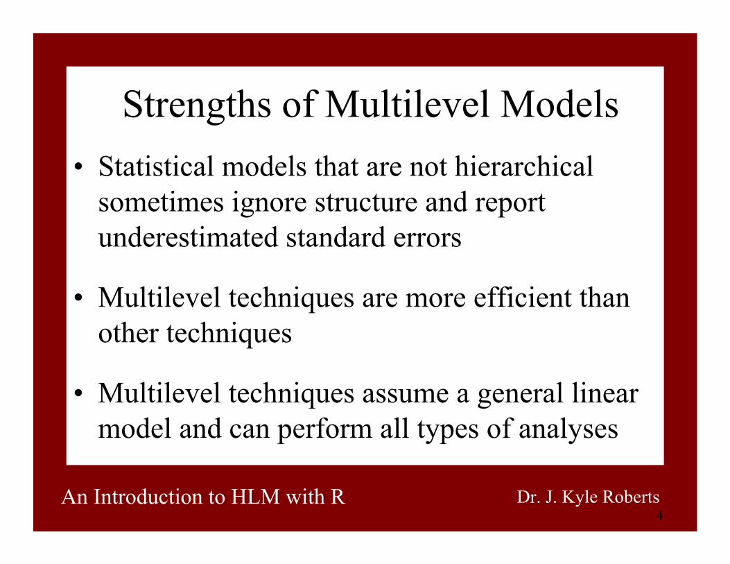
Strengths of Multilevel Models• Statistical models that are not hierarchical
sometimes ignore structure and report underestimated standard errors
• Multilevel techniques are more efficient than other techniques
• Multilevel techniques assume a general linear model and can perform all types of analyses

5An Introduction to HLM with R Dr. J. Kyle Roberts
Multilevel Examples• Students nested within classrooms• Students nested within schools• Students nested within classrooms within schools• Measurement occasions nested within subjects (repeated
measures)• Students cross-classified by school and neighborhood• Students having multiple membership in schools
(longitudinal data)• Patients within a medical center• People within households

6An Introduction to HLM with R Dr. J. Kyle Roberts
Children Nested In Families!!

7An Introduction to HLM with R Dr. J. Kyle Roberts
Do we really need HLM/MLM?
• “All data are multilevel!”• The problem of independence of
observations• The “inefficiency” of OLS techniques
8An Introduction to HLM with R Dr. J. Kyle Roberts
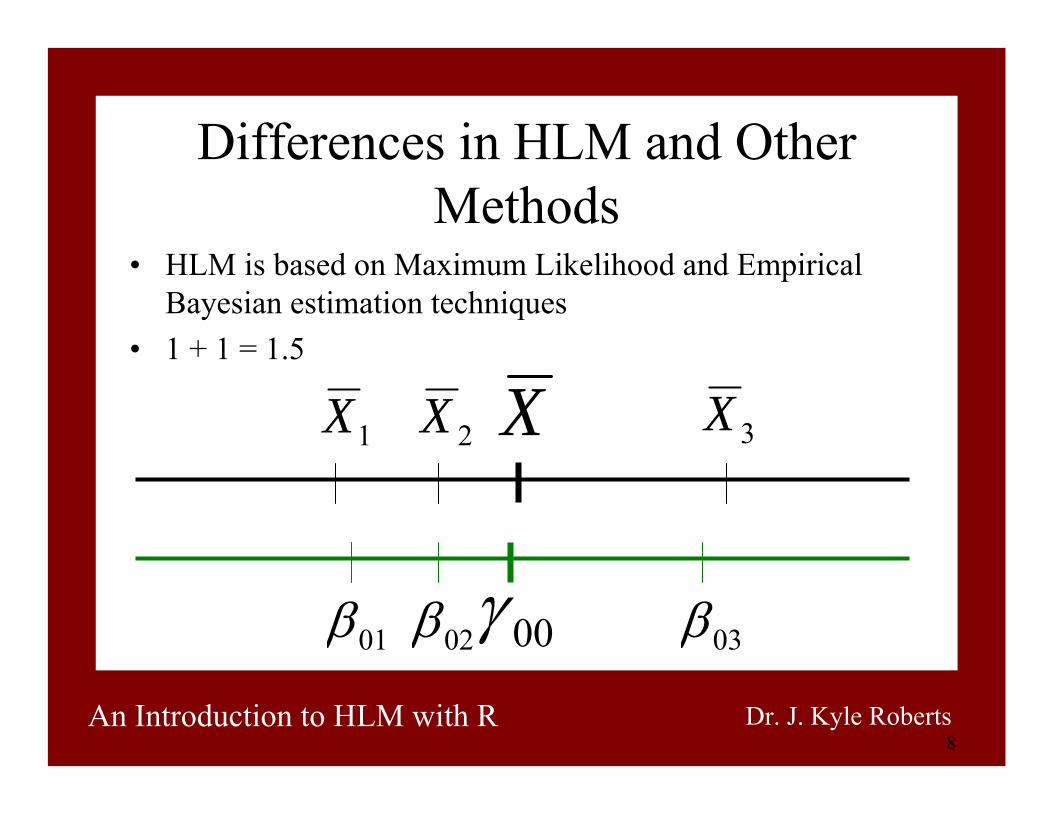
Differences in HLM and Other Methods
• HLM is based on Maximum Likelihood and Empirical Bayesian estimation techniques
• 1 + 1 = 1.5
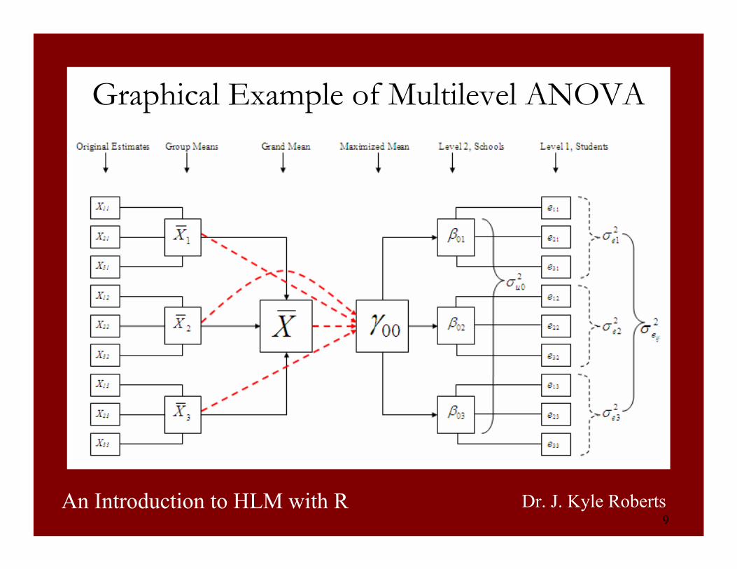
X2X 3X1X
00γ02β01β 03β
9An Introduction to HLM with R Dr. J. Kyle Roberts
Graphical Example of Multilevel ANOVA

10An Introduction to HLM with R Dr. J. Kyle Roberts
Notating the HLM ANOVA
• The full model would be:
• Level-1 model is:
• Level-2 model is:
ijjij euy ++= 000γ
ijjij ey += 0β
jj u0000 += γβ
⎪⎪⎩
⎪⎪⎨
⎧
+=
+=+=
ijjij ey
eyey
β
ββ
L21121
11111
⎪⎪⎩
⎪⎪⎨
⎧
+=
+=+=
jj u
uu
00
2002
1001
γβ
γβγβ
L

11An Introduction to HLM with R Dr. J. Kyle Roberts
Understanding Errors
2X1X X01u 02u
20uσ
11X 21X 12X 22X
11e
21e22e
12e2eσ
12An Introduction to HLM with R Dr. J. Kyle Roberts
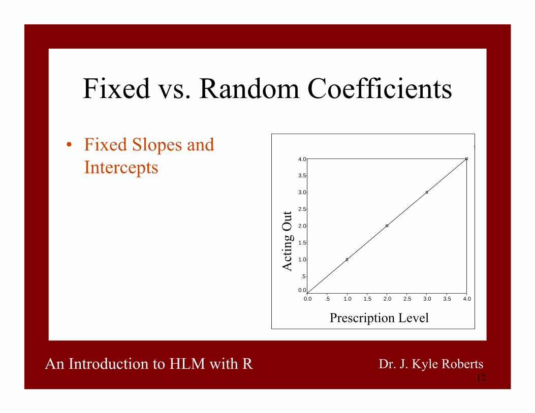
Fixed vs. Random Coefficients
• Fixed Slopes and Intercepts
Fixed Level-1 and Level-2 Coefficie
School Urbanicity
4.03.53.02.52.01.51.0.50.0
Sci
ence
Ach
ieve
men
t
4.0
3.5
3.0
2.5
2.0
1.5
1.0
.5
0.0
Prescription Level
Act
ing
Out

13An Introduction to HLM with R Dr. J. Kyle Roberts
Fixed vs. Random Coefficients
• Fixed Slopes and Intercepts
• Random Intercepts and Fixed Slopes
Random Level-1 and Fixed Level-2
School Urbanicity
4.03.02.01.00.0
Sci
ence
Ach
ieve
men
t
4.0
3.0
2.0
1.0
0.0
Prescription Level
Act
ing
Out

14An Introduction to HLM with R Dr. J. Kyle Roberts
Fixed vs. Random Coefficients
• Fixed Slopes and Intercepts
• Random Intercepts and Fixed Slopes
• Fixed Intercepts and Random Slopes
Fixed Level-1 and Random Level-2
School Urbanicity
43210S
cien
ce A
chie
vem
ent
4.0
3.0
2.0
1.0
0.0
Prescription Level
Act
ing
Out

15An Introduction to HLM with R Dr. J. Kyle Roberts
Fixed vs. Random Coefficients
• Fixed Slopes and Intercepts
• Random Intercepts and Fixed Slopes
• Fixed Intercepts and Random Slopes
• Random Slopes and Intercepts
Random Level-1 and Random Level-2
School Urbanicity
43210
Sci
ence
Ach
ieve
men
t
4.0
3.0
2.0
1.0
0.0
Prescription Level
Act
ing
Out

16An Introduction to HLM with R Dr. J. Kyle Roberts
Let’s Give This A Shot!!!
• An example where we use a child’s level of “urbanicity” (a SES composite) to predict their science achievement
• Start with Multilevel ANOVA (also called the “null model”)
ijjij ruscience ++= 000γ
Grand mean Group deviation Individual diff.

17An Introduction to HLM with R Dr. J. Kyle Roberts
Intraclass Correlation• The proportion of total variance that is between the groups
of the regression equation• “The degree to which individuals share common
experiences due to closeness in space and/or time” Kreft & de Leeuw, 1998.
• a.k.a – ICC is the proportion of group-level variance to the total variance
• LARGE ICC DOES NOT EQUAL LARGE DIFFERENCES BETWEEN MLM AND OLS (Roberts, 2002)
• Formula for ICC: 20
20
20
eu
u
σσσρ+
=
18An Introduction to HLM with R Dr. J. Kyle Roberts
Statistical Significance???
• Chi-square vs. degrees of freedom in determining model fit
• The problem with the df• Can also compute statistical significance of
variance components (only available in some packages)

19An Introduction to HLM with R Dr. J. Kyle Roberts
The Multilevel Model – Adding a Level-1 Predictor
• Consider the following 1-level regression equation:– y= a + bx + e
• y = response variable• a = intercept• b = coefficient of the response variable (slope)• x = response variable• e = residual or error due to measurement
20An Introduction to HLM with R Dr. J. Kyle Roberts
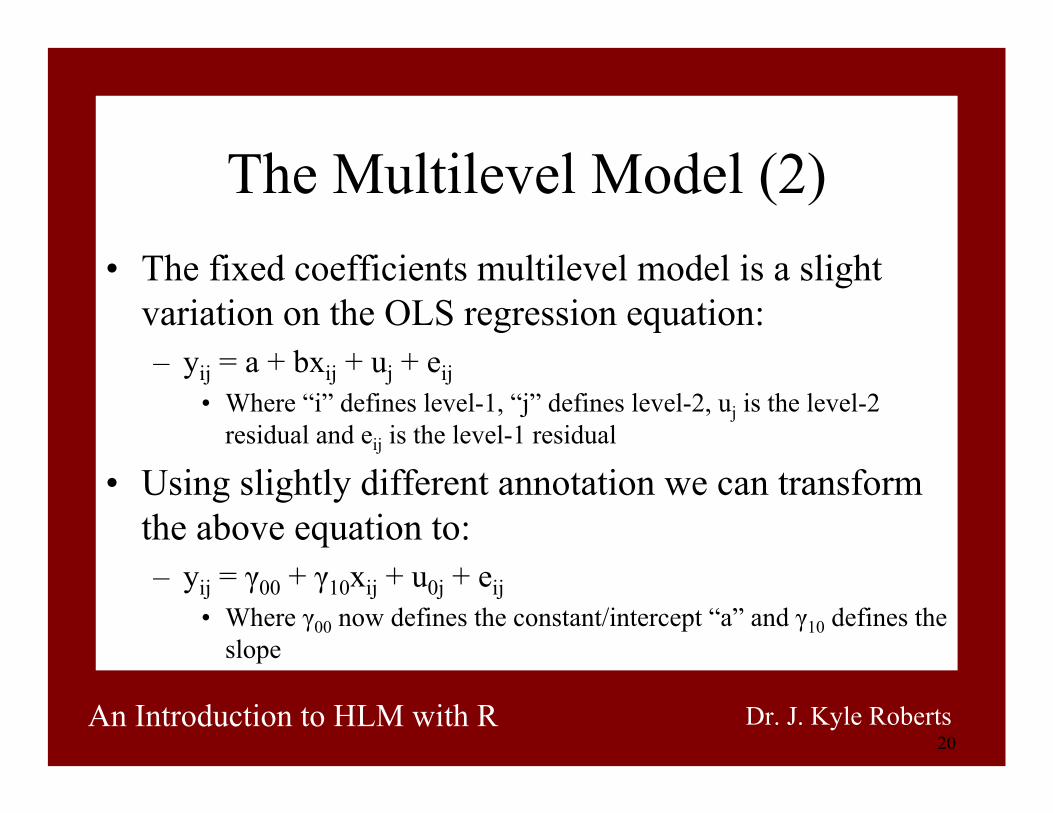
The Multilevel Model (2)• The fixed coefficients multilevel model is a slight
variation on the OLS regression equation:– yij = a + bxij + uj + eij
• Where “i” defines level-1, “j” defines level-2, uj is the level-2 residual and eij is the level-1 residual
• Using slightly different annotation we can transform the above equation to:– yij = γ00 + γ10xij + u0j + eij
• Where γ00 now defines the constant/intercept “a” and γ10 defines the slope

21An Introduction to HLM with R Dr. J. Kyle Roberts
The Multilevel Model (3)
• From the previous model:– yij = γ00 + γ10xij + u0j + eij
• We can then transform this model to:– yij = β0j + β1x1ij+eij Level-1 Model– β0j = γ00 + u0j Level-2 Model– β1j = γ10
– With variances 200 uju σ= 2
ijeije σ=

22An Introduction to HLM with R Dr. J. Kyle Roberts
Understanding Errors
ijeju0
20uσ

23An Introduction to HLM with R Dr. J. Kyle Roberts
Adding a Random Slope Component
• Suppose that we have good reason to assume that it is inappropriate to “force” the same slope for “urbanicity” on each school– Level-1 Model yij = β0jx0 + β1jx1ij + rij
– Level-2 Model β0j = γ 00 + u0j
β1j = γ10 + u1j
Complete Model ijjjij rurbanuuscience ++++= )( 110000 γγ

24An Introduction to HLM with R Dr. J. Kyle Roberts
Understanding Errors Again
21uσ ????
25An Introduction to HLM with R Dr. J. Kyle Roberts
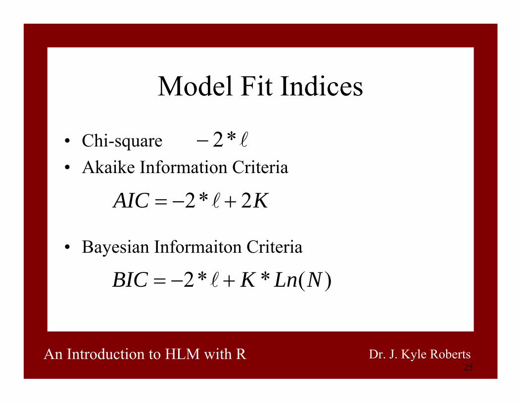
Model Fit Indices
• Chi-square • Akaike Information Criteria
• Bayesian Informaiton Criteria
l*2−
KAIC 2*2 +−= l
)(**2 NLnKBIC +−= l

26An Introduction to HLM with R Dr. J. Kyle Roberts
To Center or Not to Center•In regression, the intercept is interpreted as the expected value of the outcome variable, when all explanatory variables have the value zero
•However, zero may not even be an option in our data (e.g., Gender)
•This will be especially important when looking at cross-level interactions
•General rule of thumb: If you are estimating cross-level interactions, you should grand mean center the explanatory variables.

27An Introduction to HLM with R Dr. J. Kyle Roberts
An Introduction to R

28An Introduction to HLM with R Dr. J. Kyle Roberts
R as a Big Calculator
• Language was originally developed by AT&T Bell Labs in the 1980’s
• Eventually acquired by MathSoft who incorporated more of the functionality of large math processors
• The commands window is like a big calculator
> 2+2[1] 4
> 3*5+4[1] 19
29An Introduction to HLM with R Dr. J. Kyle Roberts
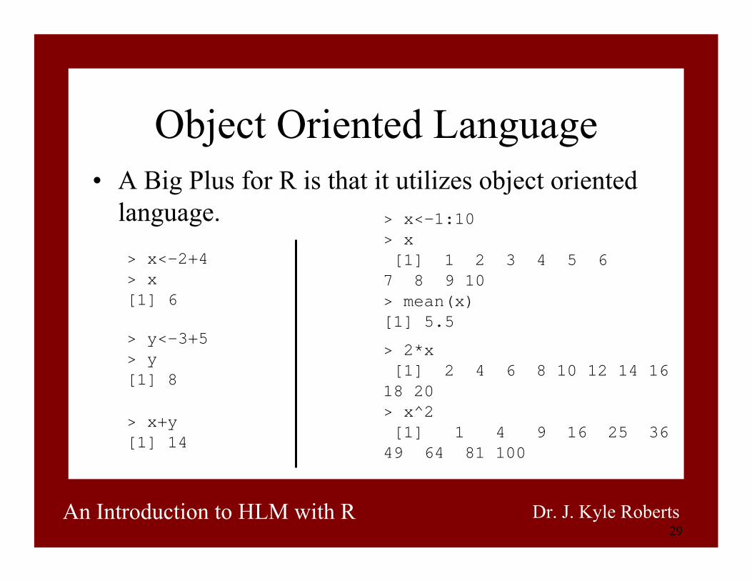
Object Oriented Language• A Big Plus for R is that it utilizes object oriented
language.> x<-2+4> x[1] 6
> y<-3+5> y[1] 8
> x+y[1] 14
> x<-1:10> x[1] 1 2 3 4 5 6 7 8 9 10> mean(x)[1] 5.5
> 2*x[1] 2 4 6 8 10 12 14 16 18 20> x^2[1] 1 4 9 16 25 36 49 64 81 100

30An Introduction to HLM with R Dr. J. Kyle Roberts
Utilizing Functions in R• R has many “built in” functions (c.f., “Language
Reference” in the “Help” menu)• Functions are commands that contain “arguments”• seq function has 4 arguments
– seq(from, to, by, length.out, along.with)
> ?seq> seq(from=1, to=100, by=10)[1] 1 11 21 31 41 51 61 71
81 91
> seq(1, 100, 10)> seq(1, by=10, length=4)[1] 1 11 21 31

31An Introduction to HLM with R Dr. J. Kyle Roberts
Making Functions in R
> squared<-function(x){x^2}> squared(5)[1] 25
> inverse<-function(x){1/x}> num<-c(1,2,3,4,5)> inverse(num)[1] 1.0000000 0.5000000 0.3333333 0.2500000 0.2000000

32An Introduction to HLM with R Dr. J. Kyle Roberts
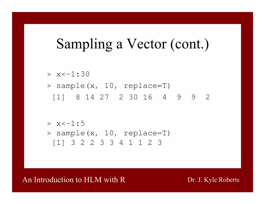
Sampling from a Single Variable
• The sample function is used to draw a random sample from a single vector of scores
• sample(x, size, replace, prob)– x = dataset– size = size of the sample to be drawn– replace = toggles on and off sampling with
replacement (default = F)– prob = vector of probabilities of same length as x
33An Introduction to HLM with R Dr. J. Kyle Roberts
Sampling a Vector (cont.)
> x<-1:30> sample(x, 10, replace=T)[1] 8 14 27 2 30 16 4 9 9 2
> x<-1:5> sample(x, 10, replace=T)[1] 3 2 2 3 3 4 1 1 2 3

34An Introduction to HLM with R Dr. J. Kyle Roberts
Rcmdr – library(Rcmdr)

35An Introduction to HLM with R Dr. J. Kyle Roberts
Reading a Dataset> example<-read.table(file, header=T)> example<-read.table(“c:/aera/example.txt”, header=T)
> head(example)
36An Introduction to HLM with R Dr. J. Kyle Roberts
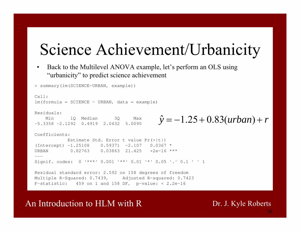
Science Achievement/Urbanicity• Back to the Multilevel ANOVA example, let’s perform an OLS using
“urbanicity” to predict science achievement> summary(lm(SCIENCE~URBAN, example))
Call:lm(formula = SCIENCE ~ URBAN, data = example)
Residuals:Min 1Q Median 3Q Max
-5.3358 -2.1292 0.4919 2.0432 5.0090
Coefficients:Estimate Std. Error t value Pr(>|t|)
(Intercept) -1.25108 0.59371 -2.107 0.0367 * URBAN 0.82763 0.03863 21.425 <2e-16 ***---Signif. codes: 0 '***' 0.001 '**' 0.01 '*' 0.05 '.' 0.1 ' ' 1
Residual standard error: 2.592 on 158 degrees of freedomMultiple R-Squared: 0.7439, Adjusted R-squared: 0.7423 F-statistic: 459 on 1 and 158 DF, p-value: < 2.2e-16
rurbany ++−= )(83.025.1ˆ
37An Introduction to HLM with R Dr. J. Kyle Roberts
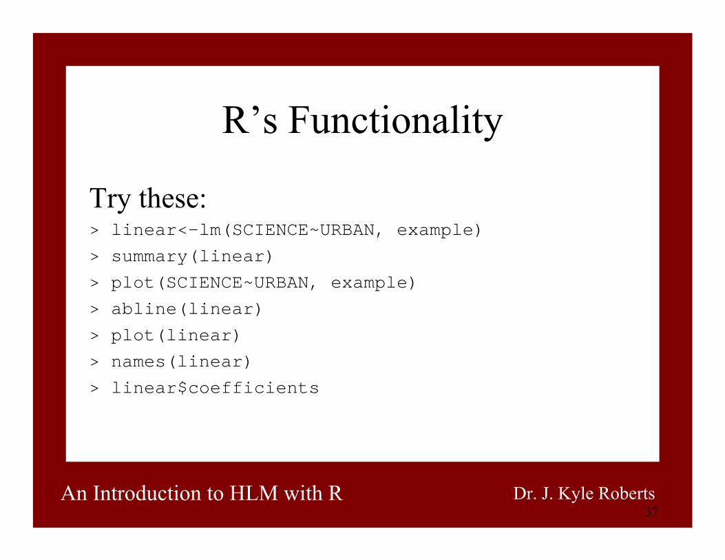
R’s Functionality
Try these:> linear<-lm(SCIENCE~URBAN, example)> summary(linear)> plot(SCIENCE~URBAN, example)> abline(linear)> plot(linear)> names(linear)> linear$coefficients

38An Introduction to HLM with R Dr. J. Kyle Roberts
lmer – library(lme4)
39An Introduction to HLM with R Dr. J. Kyle Roberts
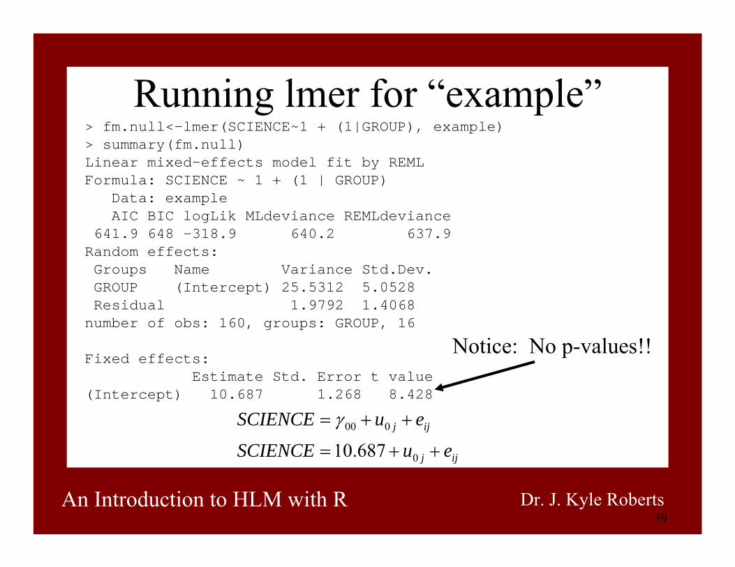
Running lmer for “example”> fm.null<-lmer(SCIENCE~1 + (1|GROUP), example)> summary(fm.null)Linear mixed-effects model fit by REML Formula: SCIENCE ~ 1 + (1 | GROUP)
Data: example AIC BIC logLik MLdeviance REMLdeviance
641.9 648 -318.9 640.2 637.9Random effects:Groups Name Variance Std.Dev.GROUP (Intercept) 25.5312 5.0528 Residual 1.9792 1.4068 number of obs: 160, groups: GROUP, 16
Fixed effects:Estimate Std. Error t value
(Intercept) 10.687 1.268 8.428
Notice: No p-values!!
ijj
ijj
euSCIENCE
euSCIENCE
++=
++=
0
000
687.10
γ

40An Introduction to HLM with R Dr. J. Kyle Roberts
bwplot(GROUP~resid(fm.null), example)
41An Introduction to HLM with R Dr. J. Kyle Roberts
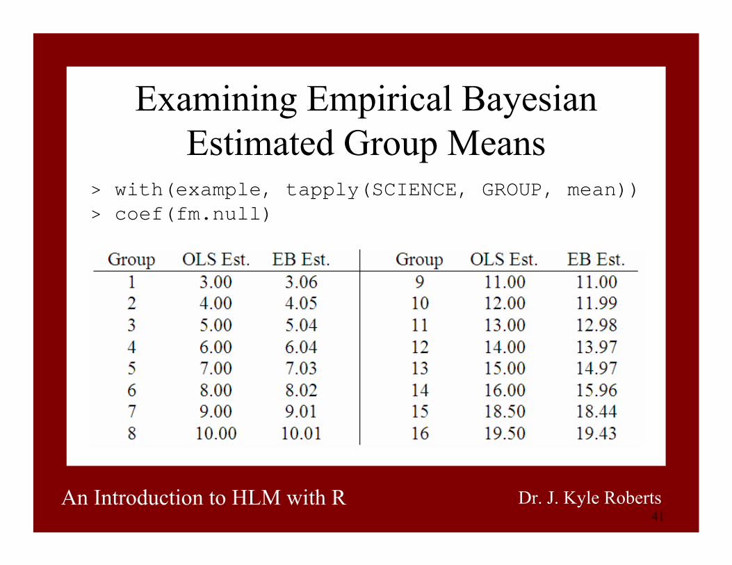
Examining Empirical Bayesian Estimated Group Means
> with(example, tapply(SCIENCE, GROUP, mean))> coef(fm.null)
42An Introduction to HLM with R Dr. J. Kyle Roberts
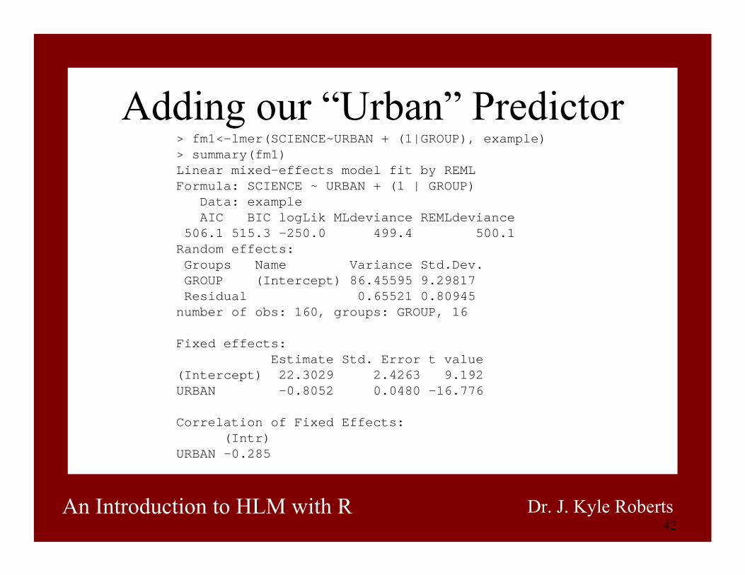
Adding our “Urban” Predictor> fm1<-lmer(SCIENCE~URBAN + (1|GROUP), example)> summary(fm1)Linear mixed-effects model fit by REML Formula: SCIENCE ~ URBAN + (1 | GROUP)
Data: example AIC BIC logLik MLdeviance REMLdeviance
506.1 515.3 -250.0 499.4 500.1Random effects:Groups Name Variance Std.Dev.GROUP (Intercept) 86.45595 9.29817 Residual 0.65521 0.80945
number of obs: 160, groups: GROUP, 16
Fixed effects:Estimate Std. Error t value
(Intercept) 22.3029 2.4263 9.192URBAN -0.8052 0.0480 -16.776
Correlation of Fixed Effects:(Intr)
URBAN -0.285
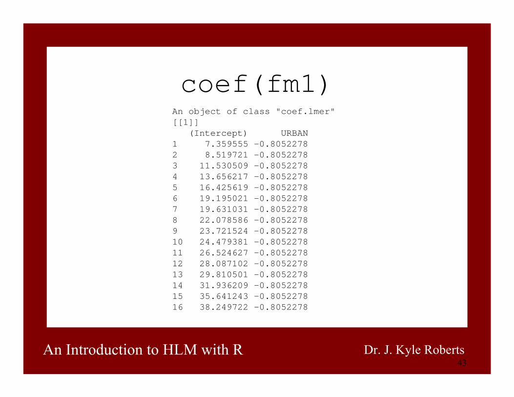
43An Introduction to HLM with R Dr. J. Kyle Roberts
coef(fm1)An object of class "coef.lmer"[[1]]
(Intercept) URBAN1 7.359555 -0.80522782 8.519721 -0.80522783 11.530509 -0.80522784 13.656217 -0.80522785 16.425619 -0.80522786 19.195021 -0.80522787 19.631031 -0.80522788 22.078586 -0.80522789 23.721524 -0.805227810 24.479381 -0.805227811 26.524627 -0.805227812 28.087102 -0.805227813 29.810501 -0.805227814 31.936209 -0.805227815 35.641243 -0.805227816 38.249722 -0.8052278

44An Introduction to HLM with R Dr. J. Kyle Roberts
Comparing Models> anova(fm.null, fm1)Data: exampleModels:fm.null: SCIENCE ~ 1 + (1 | GROUP)fm1: SCIENCE ~ URBAN + (1 | GROUP)
Df AIC BIC logLik Chisq Chi Df Pr(>Chisq) fm.null 2 644.17 650.32 -320.08 fm1 3 505.37 514.60 -249.69 140.79 1 < 2.2e-16 ***---Signif. codes: 0 '***' 0.001 '**' 0.01 '*' 0.05 '.' 0.1 ' ' 1
45An Introduction to HLM with R Dr. J. Kyle Roberts
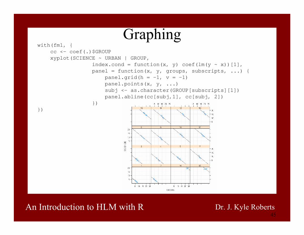
Graphingwith(fm1, {
cc <- coef(.)$GROUPxyplot(SCIENCE ~ URBAN | GROUP,
index.cond = function(x, y) coef(lm(y ~ x))[1],panel = function(x, y, groups, subscripts, ...) {
panel.grid(h = -1, v = -1)panel.points(x, y, ...)subj <- as.character(GROUP[subscripts][1])panel.abline(cc[subj,1], cc[subj, 2])
})})

46An Introduction to HLM with R Dr. J. Kyle Roberts
Adding a Random Coefficient> fm2<-lmer(SCIENCE~URBAN + (URBAN|GROUP), example)> summary(fm2)Linear mixed-effects model fit by REML Formula: SCIENCE ~ URBAN + (URBAN | GROUP)
Data: example AIC BIC logLik MLdeviance REMLdeviance
422.2 437.5 -206.1 413.2 412.2Random effects:Groups Name Variance Std.Dev. CorrGROUP (Intercept) 113.65372 10.66085
URBAN 0.25204 0.50204 -0.626 Residual 0.27066 0.52025
number of obs: 160, groups: GROUP, 16
Fixed effects:Estimate Std. Error t value
(Intercept) 22.3913 2.7176 8.239URBAN -0.8670 0.1298 -6.679
Correlation of Fixed Effects:(Intr)
URBAN -0.641

47An Introduction to HLM with R Dr. J. Kyle Roberts
coef(fm2)An object of class "coef.lmer"[[1]]
(Intercept) URBAN1 7.038437 -0.74686192 8.901233 -0.87427083 11.668557 -0.82278914 15.130206 -0.96072405 16.185638 -0.78492626 26.029030 -1.29699417 24.550979 -1.17804608 24.894060 -0.99295899 31.570587 -1.302020110 26.967287 -0.965713811 30.982799 -1.070541912 36.360597 -1.277938713 31.267775 -0.884302114 41.202393 -1.273113215 12.723743 0.271085616 12.787665 0.2879866

48An Introduction to HLM with R Dr. J. Kyle Roberts
Graphingwith(fm2, {
cc <- coef(.)$GROUPxyplot(SCIENCE ~ URBAN | GROUP,
index.cond = function(x, y) coef(lm(y ~ x))[1],panel = function(x, y, groups, subscripts, ...) {
panel.grid(h = -1, v = -1)panel.points(x, y, ...)subj <- as.character(GROUP[subscripts][1])panel.abline(cc[subj,1], cc[subj, 2])
})})

49An Introduction to HLM with R Dr. J. Kyle Roberts
Comparing Models Again> anova(fm.null, fm1, fm2)Data: exampleModels:fm.null: SCIENCE ~ 1 + (1 | GROUP)fm1: SCIENCE ~ URBAN + (1 | GROUP)fm2: SCIENCE ~ URBAN + (URBAN | GROUP)
Df AIC BIC logLik Chisq Chi Df Pr(>Chisq) fm.null 2 644.17 650.32 -320.08 fm1 3 505.37 514.60 -249.69 140.79 1 < 2.2e-16 ***fm2 5 423.22 438.60 -206.61 86.15 2 < 2.2e-16 ***---Signif. codes: 0 '***' 0.001 '**' 0.01 '*' 0.05 '.' 0.1 ' ' 1
50An Introduction to HLM with R Dr. J. Kyle Roberts
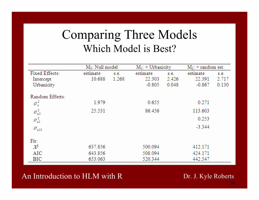
Comparing Three ModelsWhich Model is Best?
51An Introduction to HLM with R Dr. J. Kyle Roberts
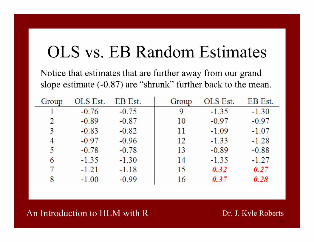
OLS vs. EB Random EstimatesNotice that estimates that are further away from our grand slope estimate (-0.87) are “shrunk” further back to the mean.

52An Introduction to HLM with R Dr. J. Kyle Roberts
R2 in HLM
2|
2|
2|2
1be
mebeRσσσ −
= 2|0
2|0
2|02
2bu
mubuRσ
σσ −=
Level-1 Equation Level-2 Equation
863.979.1
271.0979.121 =
−=R 386.2
531.25456.86531.252
2 −=−
=R
??? -238% Variance Explained???
53An Introduction to HLM with R Dr. J. Kyle Roberts
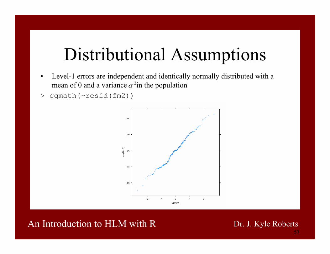
Distributional Assumptions• Level-1 errors are independent and identically normally distributed with a
mean of 0 and a variance in the population> qqmath(~resid(fm2))
2σ

54An Introduction to HLM with R Dr. J. Kyle Roberts
Distributional Assumptions• Level-1 predictor is independent of Level-1 errors> with(fm2, xyplot(resid(.) ~ fitted(.)))

55An Introduction to HLM with R Dr. J. Kyle Roberts
An Example for Homework
• http://www.hlm-online.com/datasets/education/• Look at Dataset 2 (download dataset from online)• Printout is in your packet
56An Introduction to HLM with R Dr. J. Kyle Roberts
Other Software Packages for HLM Analysis
• Good Reviews at http://www.cmm.bristol.ac.uk/– MLwiN– SAS – PROC MIXED, PROC NLMIXED, GLIMMIX– S-PLUS – lme, nlme, glme– Mplus– SPSS – Version 12 and later– STATA