Embed Size (px)
Citation preview
INTRODUCTION TO IMAGERECONSTRUCTION ANDINVERSE PROBLEMS
Eric ThiebautObservatoire de Lyon (France)
Abstract Either because observed images are blurred by the instrument and trans-fer medium or because the collected data (e.g. in radio astronomy) arenot in the form of an image, image reconstruction is a key problem inobservational astronomy. Understanding the fundamental problems un-derlying the deconvolution (noise amplification) and the way to solvefor them (regularization) is the prototype to cope with other kind ofinverse problems.
Keywords: image reconstruction, deconvolution, inverse problems, regularization.
1.1 Image formation
1.1.1 Standard image formation equation
For an incoherent source, the observed image y(s) in a direction s isgiven by the standard image formation equation:
y(s) =
∫
h(s|s′)x(s′) ds′ + n(s) (1)
where x(s′) is the object brightness distribution, h(s|s′) is the instrumen-tal point spread function (PSF), and n(s) accounts for the noise (sourceand detector). The PSF h(s|s′) is the observed brightness distributionin the direction s for a point source located in the direction s′.
Figure 1 shows the simulation of a galaxy observed with a PSF whichis typical of an adaptive optics system. The noisy blurred image in Fig. 1will be used to compare various image reconstruction methods describedin this course.
2
? 7→
+ noise 7→
Figure 1. Simulation of the image of a galaxy. From top-left to bottom-right:true object brightness distribution, PSF (instrument + transfer medium), noiselessblurred image, noisy blurred image. The PSF image was kindly provided by F. andC. Roddier.
1.1.2 Discrete form of image formation equation
For discretized data (e.g. pixels), Eq. (1) can be written in matrixform:
y = H · x + n (2)
where H is the response matrix, y, x and n are the data, object bright-ness distribution and noise vectors. These vectors have the same layout;for instance, the data vector corresponding to a N×N image writes:
y = [y(1, 1), y(2, 1), . . . , y(N, 1), y(1, 2), . . . , y(N, 2), . . . , y(N,N)]T .
1.1.3 Shift invariant PSF
Within the isoplanatic patch of the instrument and transfer medium,the PSF can be assumed to be shift invariant:
h(s|s′) = h(s− s′) , (3)
for ‖s− s′‖ small enough. In this case, the image formation equationinvolves a convolution product:
y(s) =
∫
h(s− s′)x(s′) ds′ + n(s) (4a)
FT−→ y(u) = h(u) x(u) + n(u) (4b)
Introduction to Image Reconstruction and Inverse Problems 3
where the hats denote Fourier transformed distributions and u is thespatial frequency. The Fourier transform h(u) of the PSF is called themodulation transfer function (MTF).
In the discrete case, the convolution by the PSF is diagonalized byusing the discrete Fourier transform (DFT):
yu = hu xu + nu (5)
where index u means u-th spatial frequency u of the discrete Fouriertransformed array.
1.1.4 Discrete Fourier transform
The 1-D discrete Fourier transform (DFT) of a vector x is defined by:
xu =N−1∑
k=0
xk e−2 i π u k/N FT←− xk =1
N
N−1∑
u=0
xu e+2 iπ uk/N
where i ≡√−1 and N is the number of elements in x. The N × N
discrete Fourier transform (2-D DFT) of x writes:
xu,v =∑
k,l
xk,l e−2 iπ (u k+v l)/N FT←− xk,l =
1
N2
∑
u,v
xu e+2 iπ (u k+v l)/N
where N is the number of elements along each dimension. Using matrixnotation:
x = F · x FT←− x = F−1 · x =1
NpixelFH · x
where Npixel is the number of elements in x, and FH is the conjugatetranspose of F given by (1-D case):
Fu,k ≡ exp(−2 iπ u k/N) .
In practice, DFT’s can be efficiently computed by means of fast Fouriertransforms (FFT’s).
1.2 Direct inversion
Considering the diagonalized form (5) of the image formation equa-tion, a very tempting solution is to perform straightforward direct in-version in the Fourier space and then Fourier transform back to get the
4
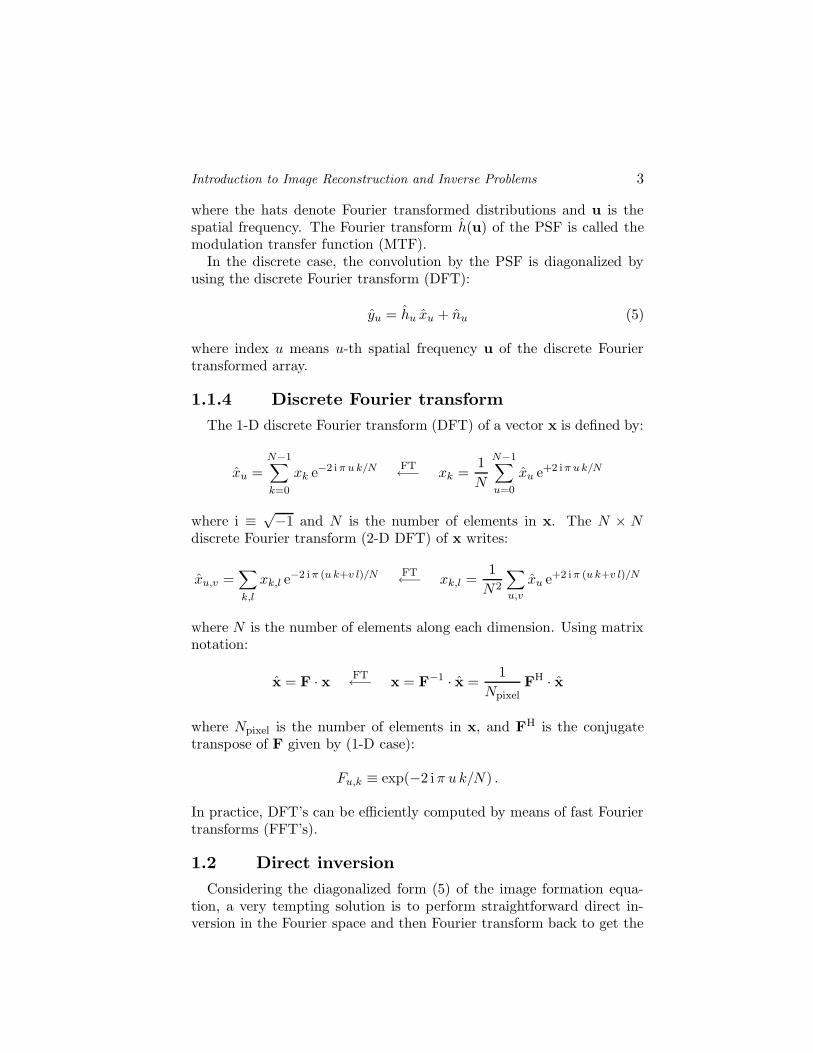
deconvolved image. In other words:
x(direct) = FFT−1
FFT
FFT
=
The result is rather disappointing: the deconvolved image is even worsethan the observed one! It is easy to understand what happens if weconsider the Fourier transform of the direct solution:
x(direct)u = yu/hu = xu + nu/hu (6)
which shows that, in the direct inversion, the perfect (but unknown)
solution xu get corrupted by a term nu/hu due to noise. In this latter
term, division by small values of the MTF hu, for instance at high fre-quencies where the noise dominates the signal (see Fig. 2a), yields verylarge distorsions. Such noise amplification produces the high frequencyartifacts displayed by the direct solution.
Instrumental transmission (convolution by the PSF) is always asmoothing process whereas noise is usually non-negligible at high fre-quencies, the noise amplification problem therefore always arises in de-convolution. This is termed as ill-conditioning in inverse problem theory.
1.3 Truncated frequencies
A crude way to eliminate noise amplification is to use a suitable cutofffrequency ucutoff and to write the solution as:
x(cutoff)u =
yu
hu
for |u| < ucutoff
0 for |u| ≥ ucutoff
(7)
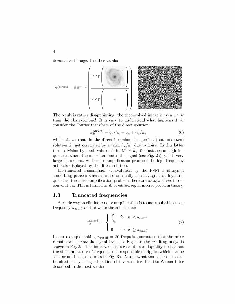
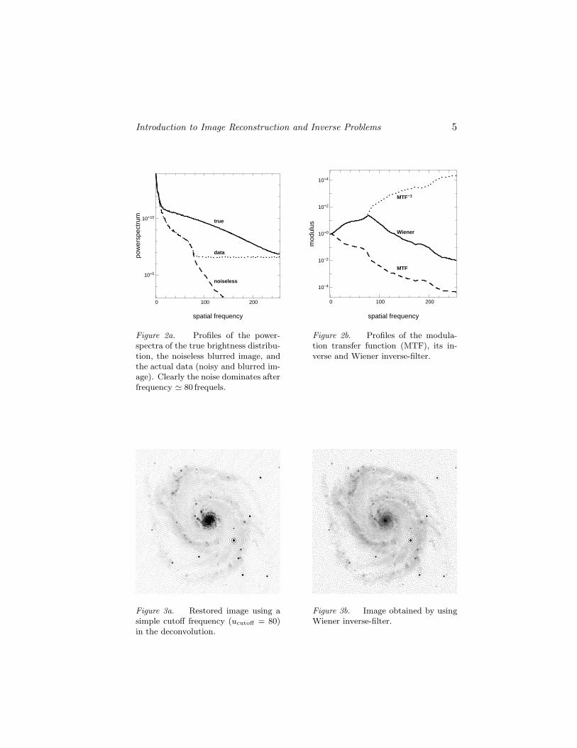
In our example, taking ucutoff = 80 frequels guarantees that the noiseremains well below the signal level (see Fig. 2a); the resulting image isshown in Fig. 3a. The improvement in resolution and quality is clear butthe stiff truncature of frequencies is responsible of ripples which can beseen around bright sources in Fig. 3a. A somewhat smoother effect canbe obtained by using other kind of inverse filters like the Wiener filterdescribed in the next section.
Introduction to Image Reconstruction and Inverse Problems 5
true
data
noiseless
0 100 200
10+5
10+10
spatial frequency
pow
ersp
ectr
um
Figure 2a. Profiles of the power-spectra of the true brightness distribu-tion, the noiseless blurred image, andthe actual data (noisy and blurred im-age). Clearly the noise dominates afterfrequency ' 80 frequels.
MTF
MTF−1
Wiener
0 100 200
10−4
10−2
10+0
10+2
10+4
spatial frequencym
odul
us
Figure 2b. Profiles of the modula-tion transfer function (MTF), its in-verse and Wiener inverse-filter.
Figure 3a. Restored image using asimple cutoff frequency (ucutoff = 80)in the deconvolution.
Figure 3b. Image obtained by usingWiener inverse-filter.
6
1.4 Wiener inverse-filter
The Wiener inverse-filter is derived from the following two criteria:
The solution is given by applying a linear filter f to the data andthe Fourier transform of the solution writes:
x(Wiener)u ≡ f (Wiener)
u yu . (8)
The expected value of the quadratic error with respect to the trueobject brightness distribution must be as small as possible:
f (Wiener) = arg minf
E{∥
∥
∥x(Wiener) − x(true)∥
∥
∥
2}
(9)
where E{x} is the expected value of x. For those not familiar withthis notation,
arg minf
φ(f)
is the element f which minimizes the value of the expression φ(f).
To summarize, Wiener inverse-filter is the linear filter which insures thatthe result is as close as possible, on average and in the least squares sense,to the true object brightness distribution.
In order to derive the expression of the filter, we write the expectedvalue ε of the quadratic error:
ε ≡ E{∥
∥
∥x(Wiener) − x(true)∥
∥
∥
2}
= E{
∑
k
(
x(Wiener)k − x
(true)k
)2}
by Parseval’s theorem (in its discrete form):
ε =1
NpixelE{
∑
u
∣
∣
∣x(Wiener)u − x(true)
u
∣
∣
∣
2}
=1
NpixelE{
∑
u
∣
∣
∣fu yu − x(true)u
∣
∣
∣
2}
.
The extremum of ε (actually a minimum) is reached for f such that:
∂ε
∂Re{fu}= 0 and
∂ε
∂Im{fu}= 0, ∀u .
Since the two partial derivatives of ε have real values, the minimum of εobeys:
∂ε
∂Re{fu}+ i
∂ε
∂Im{fu}= 0, ∀u
⇐⇒ E{
y?u (fu yu − xu)
}
= 0, ∀u
⇐⇒ E{
(hu xu + nu)? (fu (hu xu + nu)− xu)}
= 0, ∀u
⇐⇒ (|hu|2fu − h?
u) E{|xu|2}+ fu E{|nu|2} = 0, ∀u
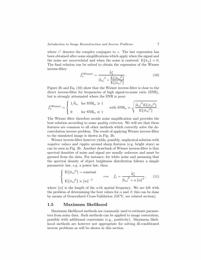
Introduction to Image Reconstruction and Inverse Problems 7
where z? denotes the complex conjugate to z. The last expression hasbeen obtained after some simplifications which apply when the signal andthe noise are uncorrelated and when the noise is centered: E{nu} = 0.The final relation can be solved to obtain the expression of the Wienerinverse-filter:
f (Wiener)u =
h?u
|hu|2+
E{|nu|2}E{|xu|2}
. (10)
Figure 2b and Eq. (10) show that the Wiener inverse-filter is close to thedirect inverse-filter for frequencies of high signal-to-noise ratio (SNR),but is strongly attenuated where the SNR is poor:
f (Wiener)u '
1/hu for SNRu � 1
0 for SNRu � 1with SNRu ≡
√
√
√
√
|hu|2E{|xu|2}
E{|nu|2}.
The Wiener filter therefore avoids noise amplification and provides thebest solution according to some quality criterion. We will see that thesefeatures are common to all other methods which correctly solve the de-convolution inverse problem. The result of applying Wiener inverse-filterto the simulated image is shown in Fig. 3b.
Wiener inverse-filter however yields, possibly, unphysical solution withnegative values and ripples around sharp features (e.g. bright stars) ascan be seen in Fig. 3b. Another drawback of Wiener inverse-filter is thatspectral densities of noise and signal are usually unknown and must beguessed from the data. For instance, for white noise and assuming thatthe spectral density of object brightness distribution follows a simpleparametric law, e.g. a power law, then:
E{|nu|2} = constant
E{|xu|2} ∝ ‖u‖−β=⇒ fu =
h?u
|hu|2+ α ‖u‖β
, (11)
where ‖u‖ is the length of the u-th spatial frequency. We are left withthe problem of determining the best values for α and β; this can be doneby means of Generalized Cross-Validation (GCV, see related section).
1.5 Maximum likelihood
Maximum likelihood methods are commonly used to estimate parame-ters from noisy data. Such methods can be applied to image restoration,possibly with additional constraints (e.g., positivity). Maximum likeli-hood methods are however not appropriate for solving ill-conditionedinverse problems as will be shown in this section.
8
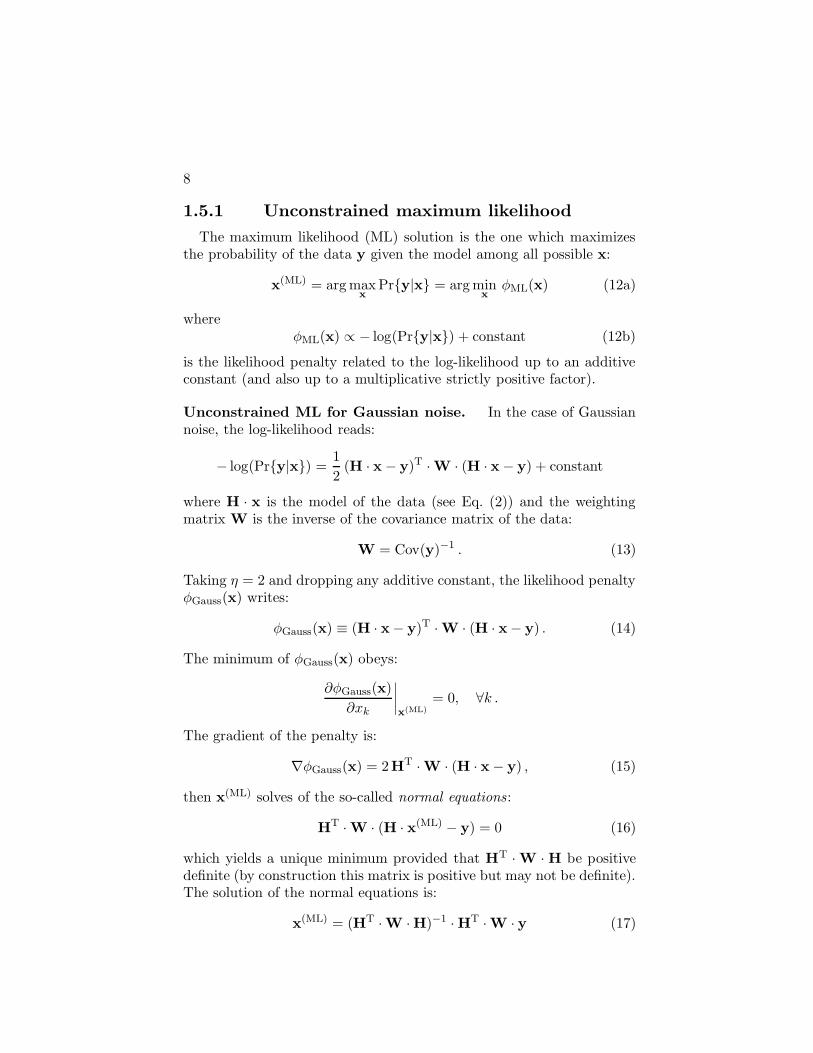
1.5.1 Unconstrained maximum likelihood
The maximum likelihood (ML) solution is the one which maximizesthe probability of the data y given the model among all possible x:
x(ML) = arg maxx
Pr{y|x} = arg minx
φML(x) (12a)
whereφML(x) ∝ − log(Pr{y|x}) + constant (12b)
is the likelihood penalty related to the log-likelihood up to an additiveconstant (and also up to a multiplicative strictly positive factor).
Unconstrained ML for Gaussian noise. In the case of Gaussiannoise, the log-likelihood reads:
− log(Pr{y|x}) =1
2(H · x− y)T ·W · (H · x− y) + constant
where H · x is the model of the data (see Eq. (2)) and the weightingmatrix W is the inverse of the covariance matrix of the data:
W = Cov(y)−1 . (13)
Taking η = 2 and dropping any additive constant, the likelihood penaltyφGauss(x) writes:
φGauss(x) ≡ (H · x− y)T ·W · (H · x− y) . (14)
The minimum of φGauss(x) obeys:
∂φGauss(x)
∂xk
∣
∣
∣
∣
x(ML)= 0, ∀k .
The gradient of the penalty is:
∇φGauss(x) = 2HT ·W · (H · x− y) , (15)
then x(ML) solves of the so-called normal equations:
HT ·W · (H · x(ML) − y) = 0 (16)
which yields a unique minimum provided that HT ·W ·H be positivedefinite (by construction this matrix is positive but may not be definite).The solution of the normal equations is:
x(ML) = (HT ·W ·H)−1 ·HT ·W · y (17)
Introduction to Image Reconstruction and Inverse Problems 9
which is the well known solution of a weighted linear least squares prob-lem1. However we have not yet proven that the ML solution is ableto smooth out the noise. We will see that this is not the case in whatfollows.
Unconstrained ML for Gaussian white noise. For Gaussianstationary noise, the covariance matrix is diagonal and proportional tothe identity matrix:
Cov(y) = diag(σ2) = σ2 I ⇐⇒ W ≡ Cov(y)−1 = σ−2 I .
Then the ML solution reduces to:
x(ML) = (HT ·H)−1 ·HT · y .
Taking the discrete Fourier transform of x(ML) yields:
x(ML)u =
h?u yu
|hu|2 =
yu
hu
(18)
which is exactly the solution obtained by the direct inversion of thediagonalized image formation equation. As we have seen before, thisis a bad solution into which the noise is amplified largely beyond anyacceptable level. The reader must not be fooled by the particular caseconsidered here for sake of simplicity (Gaussian stationary noise andDFT to approximate Fourier transforms), this disappointing result isvery general: maximum likelihood only is unable to properly solve ill-conditioned inverse problems.
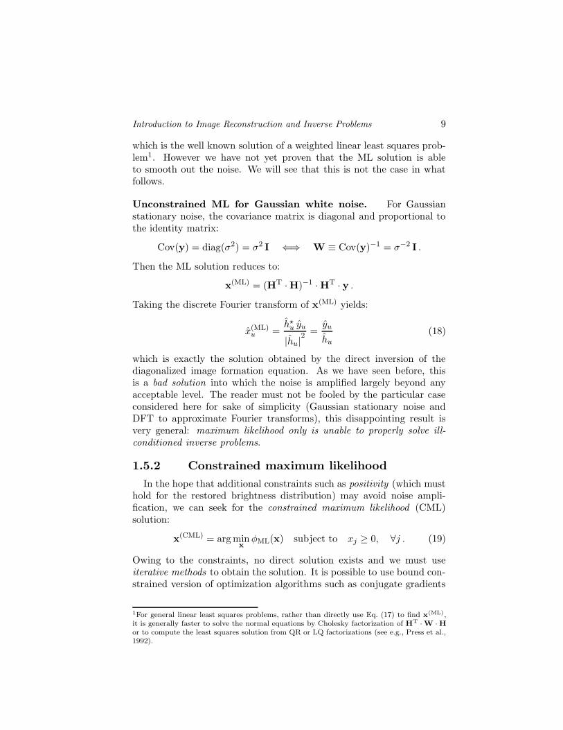
1.5.2 Constrained maximum likelihood
In the hope that additional constraints such as positivity (which musthold for the restored brightness distribution) may avoid noise ampli-fication, we can seek for the constrained maximum likelihood (CML)solution:
x(CML) = arg minx
φML(x) subject to xj ≥ 0, ∀j . (19)
Owing to the constraints, no direct solution exists and we must useiterative methods to obtain the solution. It is possible to use bound con-strained version of optimization algorithms such as conjugate gradients
1For general linear least squares problems, rather than directly use Eq. (17) to find x(ML),
it is generally faster to solve the normal equations by Cholesky factorization of HT · W · H
or to compute the least squares solution from QR or LQ factorizations (see e.g., Press et al.,1992).
10
or limited memory variable metric methods (Schwartz and Polak, 1997;Thiebaut, 2002) but multiplicative methods have also been derived toenforce non-negativity and deserve particular mention because they arewidely used: RLA (Richardson, 1972; Lucy, 1974) for Poissonian noise;and ISRA (Daube-Witherspoon and Muehllehner, 1986) for Gaussiannoise.
General non-linear optimization methods. Since the penaltymay be non-quadratic, a non-linear multi-variable optimization algo-rithm must be used to minimize the penalty function φML(x). Owingto the large number of parameters involved in image restoration (butthis is also true for most inverse problems), algorithms requiring a lim-ited amount of memory must be chosen. Finally, in case non-negativityis required, the optimization method must be able to deal with boundconstraints for the sought parameters. Non-linear conjugate gradients(CG) and limited-memory variable metric methods (VMLM or L-BFGS)meet these requirements and can be modified (using gradient projectionmethods) to account for bounds (Schwartz and Polak, 1997; Thiebaut,2002). Conjugate gradients and variable metric methods only require auser supplied code to compute the penalty function and its gradient withrespect to the sought parameters. All the images in this course whererestored using VMLM-B algorithm a limited-memory variable metricmethod with bound constraints (Thiebaut, 2002).
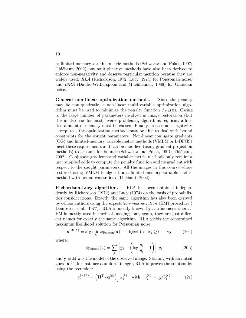
Richardson-Lucy algorithm. RLA has been obtained indepen-dently by Richardson (1972) and Lucy (1974) on the basis of probabilis-tics considerations. Exactly the same algorithm has also been derivedby others authors using the expectation-maximization (EM) procedure (Dempster et al., 1977). RLA is mostly known by astronomers whereasEM is mostly used in medical imaging; but, again, they are just differ-ent names for exactly the same algorithm. RLA yields the constrainedmaximum likelihood solution for Poissonian noise:
x(RLA) = arg minx
φPoisson(x) subject to xj ≥ 0, ∀j (20a)
where:
φPoisson(x) =∑
j
[
yj +
(
logyj
yj− 1
)]
yj (20b)
and y ≡ H·x is the model of the observed image. Starting with an initialguess x(0) (for instance a uniform image), RLA improves the solution byusing the recursion:
x(k+1)j =
(
HT · q(k))
jx
(k)j with q
(k)j = yj/y
(k)j (21)
Introduction to Image Reconstruction and Inverse Problems 11
where q(k) is obtained by element-wise division of the data y by themodel y(k) ≡ H · x(k) for the restored image x(k) at k-th iteration. Thefollowing pseudo-code implements RLA given the data y, the PSF h, astarting solution x(0) and a number of iterations n:
RLA(y, h, x(0), n)
h := FFT(h) (store MTF)for k = 0, ..., n − 1
y(k) := FFT−1(
h× FFT(x(k)))
(k-th model)
x(k+1) := x(k) × FFT−1(
h? × FFT(y/y(k)))
(new estimate)
return x(n)
where multiplications × and divisions / are performed element-wise and
h? denotes the complex conjugate of the MTF h. This pseudo-codeshows that each RLA iteration involves 4 FFT’s (plus a single FFT inthe initialization to compute the MTF).
Image Space Reconstruction Algorithm. ISRA (Daube-Witherspoon and Muehllehner, 1986) is a multiplicative and iterativemethod which yields the constrained maximum likelihood in the case ofGaussian noise. The ISRA solution is obtained using the recursion:
x(k+1)j = x
(k)j
(HT ·W · y)j
(HT ·W ·H · x(k))j(22)
A straightforward implementation of ISRA is:ISRA(y, h, W, x(0), n)
h := FFT(h) (store MTF)
r := FFT−1(
h? × FFT(W · y))
(store numerator)
for k = 0, ..., n − 1
y(k) := FFT−1(
h× FFT(x(k)))
(k-th model)
s(k) := FFT−1(
h? × FFT(W · y(k)))
(k-th denominator)
x(k+1) := x(k) × r/s(k) (new estimate)return x(n)
which, like RLA, involves 4 FFT’s per iteration. In the case of stationarynoise (W = σ−2 I), ISRA can be improved to use only 2 FFT’s periteration:
ISRA(y, h, x(0), n)
h := FFT(h) (compute MTF)
r := FFT−1(
h? × FFT(y))
(store numerator)
for k = 0, ..., n − 1
12
s(k) := FFT−1(
|h|2 × FFT(x(k)))
(k-th denominator)
x(k+1) := x(k) × r/s(k) (new estimate)return x(n)
Multiplicative algorithms (ISRA, RLA and EM) are very popular(mostly RLA in astronomy) because they are very simple to implementand their very first iterations are very efficient. Otherwise their conver-gence is much slower than other optimization algorithms such as con-strained conjugate gradients or variable metric. For instance, the resultshown in Fig. 4c was obtained in 30 minutes of CPU time on a 1 GHzPentium III laptop by VMLM-B method, against more than 10 hoursby Richardson-Lucy algorithm.
Multiplicative methods are only useful to find a non-negative solutionand, owing to the multiplication in the recursion, they leave unchangedany pixel that happens to take zero value2.
At the cost of deriving specialized algorithms, multiplicative methodscan be generalized to other expressions of the penalty to account fordifferent noise statistics3 (Lanteri et al., 2001) and can even be used toexplicitely account for regularization (Lanteri et al., 2002).
1.5.3 Maximum likelihood summary
Constraints such as positivity may help to improve the sought solution(at least any un-physical solution is avoided) because it plays the roleof a floating support (thus limiting the effective number of significantpixels). This kind of constraints are however only effective if there areenough background pixels and the improvement is mostly located nearthe edges of the support. In fact, there may be good reasons to notuse non-negativity: e.g. because there is no significant background, orbecause a background bias exists in the raw image and has not beenproperly removed.
Figures 4b and 4c show that neither unconstrained nor non-negativemaximum likelihood approaches are able to recover a usable image. De-convolution by unconstrained/constrained maximum likelihood yieldsnoise amplification — in other words, the maximum likelihood solutionremains ill-conditioned (i.e. a small change in the data due to noisecan produce arbitrarily large changes in the solution): regularization isneeded.
2This feature is however useful to implement support constraints when the support is knownin advance.3If the exact statistics of the noise is unknown, assuming stationary Gaussian noise is howevermore robust than Poissonian (Lane, 1996).
Introduction to Image Reconstruction and Inverse Problems 13
When started with a smooth image, iteratives maximum likelihoodalgorithms can achieve some level of regularization by early stoppingof the iterations before convergence (see e.g. Lanteri et al., 1999). Inthis case, the regularized solution is not the maximum likelihood oneand it also depends on the initial solution and the number of performediterations. A better solution is to explicitly account for additional reg-ularization constraints in the penalty criterion. This is explained in thenext section.
1.6 Maximum a posteriori (MAP)
1.6.1 Bayesian approach
We have seen that the maximum likelihood solution:
x(ML) = arg maxx
Pr{y|x} ,
which maximizes the probability of the data given the model, is unableto cope with noisy data. Intuitively, what we rather want is to findthe solution which has maximum probability given the data y. Such asolution is called the maximum a posteriori (MAP) solution and reads:
x(MAP) = arg maxx
Pr{x|y} . (23)
From Baye’s theorem:
Pr{x|y} =Pr{y|x} Pr{x}
Pr{y} ,
and since the probability of the data y alone does not depend on theunknowns x, we can write:
x(MAP) = arg maxx
Pr{y|x} Pr{x} .
Taking the log-probabilities:
x(MAP) = arg minx
[
− log(Pr{y|x}) − log(Pr{x})]
.
Finally, the maximum a posteriori solves:
x(MAP) = arg minx
φMAP(x) (24a)
where the a posteriori penalty reads:
φMAP(x) = φML(x) + φprior(x) (24b)
14
with:
φML(x) = −η log Pr{y|x} + constant (24c)
φprior(x) = −η log Pr{x}+ constant (24d)
where η > 0. φML(x) is the likelihood penalty and φprior(x) is the so-called a priori penalty. These terms are detailed in what follows. Nev-ertheless, we can already see that the only difference with the maximumlikelihood approach, is that the MAP solution must minimize an addi-tional term φprior(x) which will be used to account for regularization.
1.6.2 MAP: the likelihood penalty term
We have seen that minimizing the likelihood penalty φML(x) enforcesagreement with the data. Exact expression of φML(x) should depends onthe known statistics of the noise. However, if the statistics of the noiseis not known, using a least-squares penalty is more robust (Lane, 1996).In the following, and for sake of simplicity, we will assume Gaussianstationnary noise:
φML(x) = (H · x− y)T ·W · (H · x− y)
=1
σ2
∑
k
((H · x)k − yk)2 (25a)
=1
Npixel σ2
∑
u
|hu xu − yu|2. (25b)
where the latter expression has been obtained by (discrete) Parseval’stheorem.
1.6.3 MAP: the a priori penalty term
The a priori penalty φprior(x) ∝ − log Pr{x} allows us to account foradditional constraints not carried out by the data alone (i.e. by the like-lihood term). For instance, the prior can enforce agreement with somepreferred (e.g. smoothness) and/or exact (e.g. non-negativity) propertiesof the solution. At least, the prior penalty is responsible of regularizingthe inverse problem. This implies that the prior must provide informa-tion where the data alone fail to do so (in particular in regions wherethe noise dominates the signal or where data are missing). Not all priorconstraints have such properties and the enforced a priori must be cho-sen with care. Taking into account additional a priori constraints hasalso some drawbacks: it must be realized that the solution will be biasedtoward the prior.
Introduction to Image Reconstruction and Inverse Problems 15
1.6.4 Needs of a tunable a priori
Usually the functional form of the a priori penalty φprior(x) is chosenfrom qualitative (non-deterministic) arguments, for instance:
“Since we know that noise mostly contaminates the higherfrequencies, we should favor the smoothest solution among allthe solutions in agreement with the data.”
Being qualitative, the relative strength of the a priori with respect tothe likelihood must therefore be adjustable. This can be achieved thanksto an hyperparameter µ:
φMAP(x) = φµ(x) ≡ φML(x) + µφprior(x) . (26)
Alternatively µ can be seen as a Lagrange multiplier introduced to solvethe constrained problem: minimize φprior(x) subject to φML(x) be equalto some value (see Gull’s method below). Also note that there can bemore than one hyperparameter. For instance, α and β in our parame-terized Wiener filter in Eq. (11) can be seen as such hyperparameters.
1.6.5 Smoothness prior
Because the noise usually contaminates the high frequencies, smooth-ness is a very common regularization constraint. Smoothness can beenforced if φprior(x) is some measure of the roughness of the sought dis-tribution x, for instance (in 1-D):
φroughness(x) =∑
j
[xj+1 − xj]2. (27)
The roughness can also be measured from the Fourier transform x of thedistribution x:
φprior(x) =∑
u
wu |xu|2
with spectral weights wu ≥ 0 and being a non-decreasing function of thespatial frequency, e.g.:
wu = |u|β with β ≥ 0 .
The regularized solution is easy to obtain in the case of Gaussian whitenoise if we choose a smoothness prior measured in the Fourier space. Inthis case, the MAP penalty writes:
φµ(x) = φGauss(x) + µφprior(x)
= (H · x− y)T ·W · (H · x− y) + µ∑
u
wu |xu|2
16
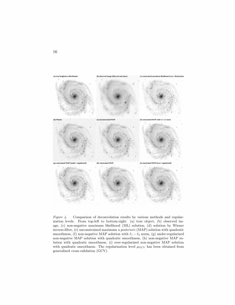
(c) constrained maximum likelihood (Lucy−Richardson)(b) observed image (blurred and noisy)(a) true brightness distribution
(d) Wiener (e) unconstrained MAP (f) constrained MAP with L1−L2 norm
(i) constrained MAP (over−regularized)(h) constrained MAP(g) constrained MAP (under−regularized)
Figure 4. Comparison of deconvolution results by various methods and regular-ization levels. From top-left to bottom-right: (a) true object, (b) observed im-age, (c) non-negative maximum likelihood (ML) solution, (d) solution by Wienerinverse-filter, (e) unconstrained maximum a posteriori (MAP) solution with quadraticsmoothness, (f) non-negative MAP solution with `1 − `2 norm, (g) under-regularizednon-negative MAP solution with quadratic smoothness, (h) non-negative MAP so-lution with quadratic smoothness, (i) over-regularized non-negative MAP solutionwith quadratic smoothness. The regularization level µGCV has been obtained fromgeneralized cross-validation (GCV).
Introduction to Image Reconstruction and Inverse Problems 17
=1
σ2
∑
j
((H · x)j − yj)2 + µ
∑
u
wu |xu|2
=1
Npixel σ2
∑
u
|hu xu − yu|2+ µ
∑
u
wu |xu|2
of which the complex gradient is:
∂φµ(x)
∂Re(xu)+ i
∂φµ(x)
∂Im(xu)=
2
Npixel σ2h?
u (hu xu − yu) + 2µwu xu .
The root of this expression is the MAP solution:
x[µ]u ≡
h?u yu
|hu|2+ µNpixel σ2 wu
(28)
Taking µNpixel σ2 wu = E{|nu|2}/E{|xu|2} or wu = ‖u‖β and α =
µNpixel σ2, this solution is identical to the one given by Wiener inverse-
filter in Eq. (11). This shows that Wiener approach is a particular casein MAP framework.
1.6.6 Other kind of regularization terms
There exist many different kind of regularization which enforce differ-ent constraints or similar constraints but in a different way.
For instance, the smoothness regularization in Eq. (27) is quadraticwith respect to the sought parameters and is a particular case ofTikhonov regularization:
φTikhonov(x) = (D · x)T · (D · x)
where D is either the identity matrix or some differential operator.Quadratic regularization may also be used in the case of a Gaussianprior or to find a solution satisfying some known correlation matrix (Tarantola and Valette, 1982):
φGP(x) = (x− p)T ·C−1x · (x− p)
where Cx is the assumed correlation matrix (when p = 0) or covariancematrix with respect to the prior p which is also the default solutionwhen there are no data.
The well-known maximum entropy method (MEM) can be imple-mented thanks to a non-quadratic regularization term which is the so-called negentropy:
φMEM(x) =∑
j
[
pj − xj + xj log
(
xj
pj
)]
18
where p is some prior distribution.Non-quadratic `1 − `2 norms applied to the spatial gradient may be
used to enforce a smoothness constraints but avoid ripples around point-like sources or sharp edges. In effect, the `1− `2 norm will prevent smalldifferences of intensity between neighbor pixels but put less constraintsfor large differences. The effectiveness of using such a norm to measurethe roughness of the sought image is shown in Fig. 4f which no longerexhibits ripples around the bright stars.
1.7 Choosing the hyperparameter(s)
In order to finally solve our inverse problem, we have to choose anadequate level of regularization. This section presents a few methods toselect the value of µ. Titterington et al. (1985) have made a comparisonof the results obtained from different methods for choosing the value ofthe hyperparameters.
1.7.1 Gull’s approach
For Gaussian noise, the MAP solution is given by minimizing:
φµ(x) = χ2(x) + µφprior(x)
where: χ2 ≡ [m(x)− y]T ·W · [m(x) − y] ,
where m(x) is the model. For a perfect model, the expected value ofχ2 is equal to the number of measurements: E{χ2} = Ndata. If theregularization level is too small, the MAP model will tend to overfit thedata resulting in a value of χ2 smaller than its expected value. On thecontrary, if the regularization level is too high, the MAP model will betoo biased by the a priori and χ2 will be larger than its expected value.These considerations suggest to choose the weight µ of the regularizationsuch that:
χ2(x[µ]) = E{χ2} = Ndata
where x[µ] is the MAP solution obtained for a given µ. In practice,this choice tends to oversmooth the solution. In fact, the model beingderived from the data, it is always biased toward the data and, even fora correct level of regularization, the expected value of χ2 must be lessthan Ndata. For a parametric model with M free parameters adjustedso as to minimize χ2, the correct formula is:
E{χ2} = Ndata −M ,
the difference Ndata −M is the so-called number of degrees of freedom.This formula cannot be directly applied to our case because the parame-ters of our model are correlated by the regularization and M � Nparam.
Introduction to Image Reconstruction and Inverse Problems 19
Gull (1989), considering that the prior penalty is used to control theeffective number of free parameters, stated that M ' µφprior(x). Fol-lowing Gull’s approach, the hyperparameter µ and the MAP solutionare obtained by:
x(Gull) = arg minx
φµ(x) subject to: φµ(x) = Ndata (29)
with φµ(x) = χ2(x) + µφprior(x) and also possibly subject to xj ≥0,∀j. This method is rarely used because it requires to have a very goodestimation of the absolute noise level.
1.7.2 Cross-validation
Cross-Validation methods make use of the fact that it is possible toestimate missing measurements when the solution of an inverse problemis obtained.
Ordinary cross-validation. Let:
x[µ,k] = arg minφµ(x|y[k]) where y[k] ≡ {yj : j 6= k} (30)
be the regularized solution obtained from the incomplete data set wherethe k-th measurement is missing; then:
y[µ,k] ≡ (H · x[µ,k])k (31)
is the predicted value of the missing data yk. The cross-validationpenalty is the weighted sum of the quadratic difference between thepredicted value and the real measurement:
CV(µ) ≡∑
k
(y[µ,k] − yk)2
σ2k
(32)
where σ2k is the variance of the k-th measurement (noise is assumed
to be uncorrelated). For a given value of the hyperparameter, CV(µ)measures the statistical ability of the inversion to predict the value ofmissing data. A good choice for the hyperparameter is the one thatminimizes CV(µ) since it would achieve the best prediction capability.CV(µ) can be re-written into a more workable expression:
CV(µ) =∑
k
(y[µ]k − yk)
2
σ2k (1− a
[µ]k,k)
2(33)
where:y[µ] = H · x[µ] (34)
20
is the model for a given µ and a[µ] is the so-called influence matrix :
a[µ]k,l =
∂y[µ]k
∂yl. (35)
Generalized cross-validation. To overcome some problems withordinary cross-validation, Golub et al. (1979) have proposed the gener-alized cross-validation (GCV) which is a weighted version of CV:
GCV(µ) =∑
k
w[µ]k
(y[µ,k] − yk)2
σ2k
=
∑
k(y[µ]k − yk)
2/σ2k
[
1− 1Npixel
∑
k a[µ]k,k
]2 . (36)
(G)CV in the case of deconvolution. In our case, i.e. gaussianwhite noise and smoothness prior, the MAP solution is:
x[µ]u ≡
h?u yu
|hu|2+ µ ru
with ru = Npixel σ2 wu.
the Fourier transform of the corresponding model is:
ˆy[µ]u ≡ hu x[µ]
u =|hu|
2yu
|hu|2+ µ ru
= q[µ]u yu with q[µ]
u =|hu|
2
|hu|2+ µ ru
and all the diagonal terms of the influence matrix are identical :
a[µ]k,k =
∂y[µ]k
∂yk=
1
Npixel
∑
u
q[µ]u .
In our case, i.e. gaussian white noise and smoothness prior, CV andGCV have the same expression:
CV(µ) = GCV(µ) =
∑
u
(
1− q[µ]u
)2|yu|2
[
1− 1Npixel
∑
u q[µ]u
]2
which can be evaluated for different values of µ in order to find itsminimum.
1.8 Myopic and blind deconvolution
So far, we considered image deconvolution assuming that the PSFwas perfectly known. In practice, this is rarely the case. For instance,when the PSF is measured by a calibration procedure, it is corrupted
Introduction to Image Reconstruction and Inverse Problems 21
by some level of noise. Moreover, if the observing conditions change,the calibrated PSF can mismatch the actual PSF. It may even be thecase that the PSF cannot be properly calibrated at all, because it isvarying too rapidly, or because there is no time or no means to do sucha calibration. What can we do to cope with that?
In this case, since the unknown are the object brightness distributionx and the actual PSF h, the MAP problem has to be restated as:
{x,h}(MAP) = arg max{x,h}
Pr{x,h|y} (37)
where the data are y = {yobj,yPSF}, yobj being the observed image ofthe object and yPSF being the calibration data. Expanding the previousequation:
{x,h}(MAP) = arg max{x,h}
Pr{x,h|y}
= arg max{x,h}
Pr{y|x,h} Pr{x,h}Pr{y}
= arg max{x,h}
Pr{y|x,h} Pr{x} Pr{h}Pr{y}
= arg max{x,h}
Pr{y|x,h} Pr{x} Pr{h}
= arg min{x,h}
(− log Pr{y|x,h} − log Pr{x} − log Pr{h})
we find that the sought PSF and object brightness distribution are aminimum of:
φmyopic(x,h) = φML(y|x,h) + µobj φobj(x) + µPSF φPSF(h) (38)
where φML(y|x,h) ∝ − log Pr{y|x,h} is the likelihood penalty andwhere φobj(x) ∝ − log Pr{x} and φpsf(h) ∝ − log Pr{h} are regulariza-tion terms enforcing the a priori constraints for the sought distributions.
Assuming Gaussian noise and if the calibration data is given by animage of a point-like source, the MAP criterion writes:
φmyopic(x,h) = (h� x− yobj)T ·Wobj · (h� x− yobj)
+(h− yPSF)T ·WPSF · (h− yPSF)
+µobj φobj(x) + µPSF φPSF(h) (39)
where � denotes convolution and where Wobj and WPSF are the weight-ing matrices for the object and PSF images respectively.
Solving such a myopic deconvolution problem is much more difficultbecause its solution is highly non-linear with respect to the data. In
22
effect, whatever are the expressions of the regularization terms, the cri-terion to minimize is no longer quadratic with respect to the parameters(due to the first likelihood term). Nevertheless, a much more impor-tant point to care of is that unless enough constraints are set by theregularization terms, the problem may not have a unique solution.
A possible algorithm for finding the solution of the myopic problemis to proceed by successive regularized deconvolutions. At every stage,a new estimate of the object is obtained by a first regularized deconvo-lution given the data, the constraints and an estimate of the PSF, thenanother regularized deconvolution is used to obtain a new estimate ofthe PSF given the constraints, the data and the previous estimate of theobject brightness distribution:
x(k+1) = arg minx
[
(h(k) � x− yobj)T ·Wobj · (h(k) � x− yobj)
+ µobj φobj(x)]
h(k+1) = arg minh
[
(h� x(k+1) − yobj)T ·Wobj · (h� x(k+1) − yobj)
+ (h− yPSF)T ·WPSF · (h− yPSF)
+ µPSF φPSF(h)]
where x(k) and h(k) are the sought distributions at k-th iteration. Suchan iterative algorithm does reduce the global criterion φMAP(x,h) butthe final solution depends on the initial guess x(0) or h(0) unless theregularization terms warrant unicity.
Myopic deconvolution has enough flexibility to account for differentcases depending on the signal-to-noise ratio of the measurements:
In the limit WPSF → +∞, the PSF is perfectly characterized bythe calibration data (i.e. h ← yPSF) and myopic deconvolutionbecomes identical to conventional deconvolution.
In the limit WPSF → 0 or if no calibration data are available,myopic deconvolution becomes identical to blind deconvolutionwhich involves to find the PSF and the brightness distribution ofthe object from only an image of the object.
Stated like this, conventional and blind deconvolution appear to be justtwo extreme cases of the more general myopic deconvolution problem.We however have seen that conventional deconvolution is easier to per-form than myopic deconvolution and we can anticipate that blind de-convolution must be far more difficult.
Introduction to Image Reconstruction and Inverse Problems 23
blind deconvolutionconvolution + noise
0
0.3
0.6
0.9
0
0.3
0.6
0.9
0
0.3
0.6
0.9
0
0.3
0.6
0.9
0
0.3
0.6
0.9
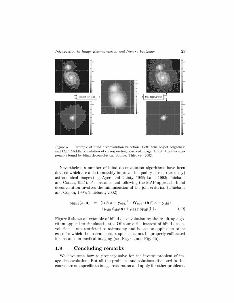
Figure 5. Example of blind deconvolution in action. Left: true object brightnessand PSF. Middle: simulation of corresponding observed image. Right: the two com-ponents found by blind deconvolution. Source: Thiebaut, 2002.
Nevertheless a number of blind deconvolution algorithms have beendevised which are able to notably improve the quality of real (i.e. noisy)astronomical images (e.g. Ayers and Dainty, 1988; Lane, 1992; Thiebautand Conan, 1995). For instance and following the MAP approach, blinddeconvolution involves the minimization of the join criterion (Thiebautand Conan, 1995; Thiebaut, 2002):
φblind(x,h) = (h� x− yobj)T ·Wobj · (h� x− yobj)
+µobj φobj(x) + µPSF φPSF(h) . (40)
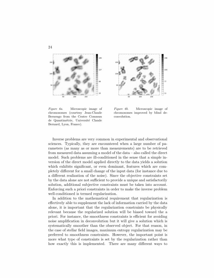
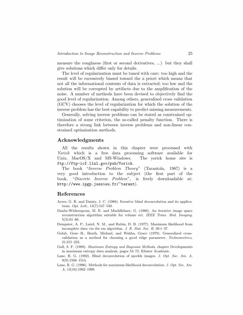
Figure 5 shows an example of blind deconvolution by the resulting algo-rithm applied to simulated data. Of course the interest of blind decon-volution is not restricted to astronomy and it can be applied to othercases for which the instrumental response cannot be properly calibratedfor instance in medical imaging (see Fig. 6a and Fig. 6b).
1.9 Concluding remarks
We have seen how to properly solve for the inverse problem of im-age deconvolution. But all the problems and solutions discussed in thiscourse are not specific to image restoration and apply for other problems.
24
50 100 150
50
100
150
10
68
127
185
Figure 6a. Microscopic image ofchromosomes (courtesy Jean-ClaudeBernengo from the Centre Communde Quantimetrie, Universite ClaudeBernard, Lyon, France).
50 100 150
50
100
150
11
77
143
208
Figure 6b. Microscopic image ofchromosomes improved by blind de-convolution.
Inverse problems are very common in experimental and observationalsciences. Typically, they are encountered when a large number of pa-rameters (as many as or more than measurements) are to be retrievedfrom measured data assuming a model of the data – also called the directmodel. Such problems are ill-conditioned in the sense that a simple in-version of the direct model applied directly to the data yields a solutionwhich exhibits significant, or even dominant, features which are com-pletely different for a small change of the input data (for instance due toa different realization of the noise). Since the objective constraints setby the data alone are not sufficient to provide a unique and satisfactorilysolution, additional subjective constraints must be taken into account.Enforcing such a priori constraints in order to make the inverse problemwell-conditioned is termed regularization.
In addition to the mathematical requirement that regularization iseffectively able to supplement the lack of information carried by the dataalone, it is important that the regularization constraints be physicallyrelevant because the regularized solution will be biased toward the apriori. For instance, the smoothness constraints is efficient for avoidingnoise amplification in deconvolution but it will give a solution which issystematically smoother than the observed object. For that reason, inthe case of stellar field images, maximum entropy regularization may bepreferred to smoothness constraints. However, the important point ismore what type of constraints is set by the regularization rather thanhow exactly this is implemented. There are many different ways to
Introduction to Image Reconstruction and Inverse Problems 25
measure the roughness (first or second derivatives, ...) but they shallgive solutions which differ only for details.
The level of regularization must be tuned with care: too high and theresult will be excessively biased toward the a priori which means thatnot all the informational contents of data is extracted; too low and thesolution will be corrupted by artifacts due to the amplification of thenoise. A number of methods have been devised to objectively find thegood level of regularization. Among others, generalized cross validation(GCV) chooses the level of regularization for which the solution of theinverse problem has the best capability to predict missing measurements.
Generally, solving inverse problems can be stated as constrained op-timization of some criterion, the so-called penalty function. There istherefore a strong link between inverse problems and non-linear con-strained optimization methods.
Acknowledgments
All the results shown in this chapter were processed withYorick which is a free data processing software available forUnix, MacOS/X and MS-Windows. The yorick home site isftp://ftp-icf.llnl.gov/pub/Yorick.
The book “Inverse Problem Theory” (Tarantola, 1987) is avery good introduction to the subject (the first part of thebook, “Discrete Inverse Problem”, is freely downloadable at:http://www.ipgp.jussieu.fr/~tarant).
References
Ayers, G. R. and Dainty, J. C. (1988). Iterative blind deconvolution and its applica-tions. Opt. Lett., 13(7):547–549.
Daube-Witherspoon, M. E. and Muehllehner, G. (1986). An iterative image spacereconstruction algorithm suitable for volume ect. IEEE Trans. Med. Imaging,5(2):61–66.
Dempster, A. P., Laird, N. M., and Rubin, D. B. (1977). Maximum likelihood fromincomplete data via the em algorithm. J. R. Stat. Soc. B, 39:1–37.
Golub, Gene H., Heath, Michael, and Wahba, Grace (1979). Generalized cross-validation as a method for choosing a good ridge parameter. Technometrics,21:215–223.
Gull, S. F. (1989). Maximum Entropy and Bayesian Methods, chapter Developmentsin maximum entropy data analysis, pages 53–72. Kluwer Academic.
Lane, R. G. (1992). Blind deconvolution of speckle images. J. Opt. Soc. Am. A,9(9):1508–1514.
Lane, R. G. (1996). Methods for maximum-likelihood deconvolution. J. Opt. Soc. Am.
A, 13(10):1992–1998.
26
Lanteri, H., Soummer, R., and Aime, C. (1999). Comparison between ISRA and RLAalgorithms. Use of a Wiener Filter based stopping criterion. A&AS, 140:235–246.
Lanteri, H., Roche, M., and Aime, C. (2002). Penalized maximum likelihood imagerestoration with positivity constraints: multiplicative algorithms. Inverse Prob-
lems, 18:1397–1419.
Lanteri, H., Roche, M., Cuevas, O., and Aime, C. (2001). A general method to de-vise maximum-likelihood signal restoration multiplicative algorithms with non-negativity constraints. Signal Processing, 81:945–974.
Lucy, L. B. (1974). An iterative technique for the rectification of observed distribu-tions. ApJ, 79(6):745–754.
Press, W. H., Teukolsky, S. A., Vetterling, W. T., and Flannery, B. P. (1992). Nu-
merical Recipes in C. Cambridge University Press, 2nd edition.
Richardson, W. H. (1972). Bayesian-based iterative method of image restauration. J.
Opt. Soc. Am., 62(1):55–59.
Schwartz, A. and Polak, E. (1997). Family of projected descent methods for optimiza-tion problems with simple bounds. Journal of Optimization Theory and Applica-
tions, 92(1):1–31.
Tarantola, A. (1987). Inverse Problem Theory. Elsevier.
Tarantola, A. and Valette, B. (1982). Generalized nolinear inverse problems solved us-ing the least squares criterion. Reviews of Geophysics and Space Physics, 20(2):219–232.
Thiebaut, E. and Conan, J.-M. (1995). Strict a priori constraints for maximum like-lihood blind deconvolution. J. Opt. Soc. Am. A, 12(3):485–492.
Thiebaut, Eric (2002). Optimization issues in blind deconvolution algorithms. InStarck, Jean-Luc and Murtagh, Fionn D., editors, Astronomical Data Analysis
II, volume 4847, pages 174–183. SPIE.
Titterington, D. M. (1985). General structure of regularization procedures in imagereconstruction. Astron. Astrophys., 144:381–387.