Introduction to Information Theory

1B. Škorić, Physical Aspects of Digital Security, Chapter 2

Information theory

• What is it? - formal way of counting “information” bits

• Why do we need it? - often used in crypto - best way to talk about physical sources

of randomness

2

Measuring ignorance

Experiment X with unpredictable outcome • known possible outcomes xi • known probabilities pi. !!!We want to measure the “unpredictability” of the experiment • should increase with #outcomes • should be maximal for uniform pi

3

Measuring ignorance

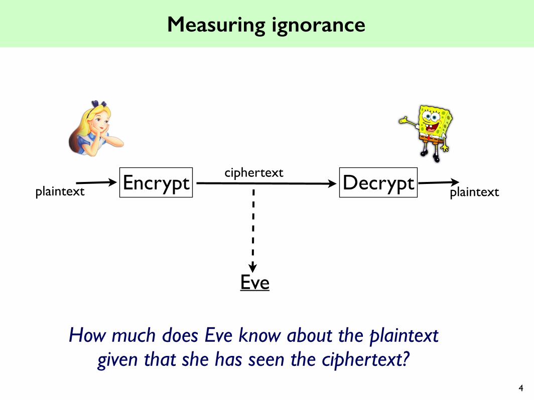
Encrypt Decryptplaintext plaintextciphertext

Eve

How much does Eve know about the plaintext given that she has seen the ciphertext?

4

Measuring common knowledge

data⨁

data’

noise

How much of the info that Alice sends does actually reach Bob? (“channel capacity”)

5

Data compression

How far can a body of data be compressed?

Bla bla blather bla dinner bla bla bla bla

blep bla bla bla bla bla bla bla tonight bla blabla bla blather bla bla blather bla

bla blab blaYawn

dinner tonight

6

plaatje

Claude Shannon (1916 - 2001) !!

Groundbreaking work in 19487

Shannon entropy

Notation: H(X) or H( {p1,p2, ...} ) !Formal requirements for counting information bits • Sub-additivity: H(X,Y) ⩽ H(X) + H(Y)

- equality only when X and Y independent • Expansibility: extra outcome xj with pj=0 has no effect • Normalization:

- entropy of (1/2, 1/2) is 1 bit; of (1,0,0, ...) is zero. !

Unique expression satisfying all requirements:

H(X) = −Σx px log2(px)8

Examples of Shannon entropy

H(X) = −Σx px log(px)

• Uniform distribution X∼(1/n, ..., 1/n). H(X) = log n.

• Binary entropy function. X∼(p, 1-p). h(p) = h(1-p) = −p log p − (1-p) log(1-p)

2.2. SHANNON ENTROPY 9

2.2 Shannon entropy

2.2.1 Measuring the amount of information

It is very useful to have a good measure for the ‘amount of real information’ in a random variable. Itis intuitively clear that, for instance, the roll of a 12-sided die carries more information than a coinflip, and that a biased coin (being more predictable) has less information than a fair coin. Finding agood way of measuring this, however, is not completely trivial. Obviously, ‘predictability’ reducesinformation. The amount of information grows with the number of possible outcome values of theRV. If all outcomes are equally likely, there is more information than if one of them has a verylarge probability. From such intuition we can make a list of desirable formal properties:

1. Additivity: The information content of a set of independent RVs must be the sum of theindividual information contents.

2. Sub-additivity: The total information content of two jointly distributed RVs cannot exceedthe sum of their separate informations.

3. Expansibility: Adding an extra outcome to the set of possible outcomes of the experiment,with probability 0, does not a�ect the information.

4. Normalization: The distribution { 12 , 1

2} has an information content of 1 bit.

5. The distribution {p, 1� p} for p ⌅ 0 has zero information.

It turns out that there is only one measure that satisfies all these requirements. It is called Shannonentropy. Let X ⇧ X , let X ⇤ P and px := P(x). The Shannon entropy of X is defined as

H(X) =�

x�X px log21px

. (2.11)

Exercise 2.7 Show that the Shannon entropy (2.11) has the following properties.

• Properties 1,3, 4 and 5 above.

• If the distribution is uniform, then H(X) = log2 |X |.

The formula (2.11) can be interpreted as E[log2(1/px)], i.e. the average of all the ‘uniform’entropies log2(1/px).

Example 2.10 Consider an experiment with two possible outcomes, one with probability p andthe other with probability 1� p. The entropy of the distribution {p, 1� p} is

h(p) := p log1p

+ (1� p) log1

1� p.

The function h is called the binary entropy function.

9

Mini quiz

H(X) = −Σx px log(px)

X∼(1/2, 1/4, 1/4). Compute H(X).

• Which yes/no questions would you ask to quickly

determine the outcome of the experiment?

• How many questions do you need on average?

10

Interpretation of Shannon entropy

1) Average number of binary questions needed to decide on outcome of experiment (lower bound)

2) Lower bound on compression size 3) Theory of ‘types’:

• Given pmf S = (s1,...,sq); N independent experiments;

• Type T ≔ sequences with exactly ni = N si occurrences of i.

• t ∈ T.

10 CHAPTER 2. INFORMATION THEORY

A very useful way of thinking about Shannon entropy is as follows. H(X) is a lower bound onthe average number of binary (yes/no) questions that you need to ask about the RVin order to learn the outcome x. Every binary question corresponds to one bit of information.

Example 2.11 Consider a fair 8-sided die. You could first ask if x lies in the range 1–4 or 5–8.The 2nd question could be to ask if x lies in the lowest two values of that range; the 3rd questionif x is the lowest value of the remaining two possibilities. This exactly matches log2 8 = 3.

Example 2.12 Consider a fair six-sided die. The first question is if x lies in the range 1–3 or4–6. The second question is if x is the lowest element of this range. With prob. 2/3, an extraquestion will be needed. The average is 1

3 · 2 + 23 · 3 = 8

3 ⇤ 2.67 questions, which is more thanlog2 6 ⇤ 2.58.

Exercise 2.8 In example 2.12, what could you do to get closer to the theoretical bound log2 6?

Similarly, H(X) is a lower bound on the average length of the shortest description ofX. In other words, an optimal compression algorithm for X will, on average, yield compressionsthat have length at least H(X).Yet another way to look at Shannon entropy comes from ‘typical sequences’. Consider a sequenceof n independent experiments X. The asymptotic equipartition theorem states that most of theprobability mass is contained in approximately 2nH(X) ‘typical’ sequences, and that these typicalsequences have equal probability (⇤ 2�nH(X)) of occurring.A slightly easier formulation of the same statement is as follows. Consider a distribution S ={s1, . . . , sq} with q ⌅ N, si = ni/N (where ni ⌅ N) and

�qi=1 si = 1. A string X ⌅ [q]N is

randomly generated in such a way that the symbols Xi are independently drawn from [q] accordingto the distribution S. We define the ‘type’ T as the set of all strings in [q]N that contain preciselyn1 ones, n2 twos, . . . nq ‘q’s. For any fixed t ⌅ T , it then holds that

Pr[X = t] =q⇥

i=1

snii =

q⇥

i=1

sNsii = 2

Pi Nsi log si = 2�NH(S). (2.12)

The probability Pr[X = t] is the same for all t ⌅ T . When N is very large, the probability of Xbeing in T is overwhelming.

Exercise 2.9 Show that the size of T is 2NH(S)�O(log N). Hint: Use Stirling’s approximationn! ⇤

⌥2�n (n/e)n.

2.2.2 History of the entropy concept

The concept of entropy first arose in thermodynamics, in the equation F = U � TS, where F isthe (Helmholtz) free energy, U the total energy, T the temperature and S the entropy. The freeenergy is defined as the amount of energy that can be converted to useful work in a closed systemat constant temperature and volume.Boltzmann’s statistical mechanics approach [] led to the understanding that S is related to thenumber of degrees of freedom of the particles making up the physical system, or in other words thenumber of micro-states (complete specification of all particle states) per macro-state (global state,e.g. chracterized by only a handful parameters such as volume, pressure, temperature). If pi is theprobability that the i’th micro-state occurs, given a fixed macro-state, then S = k

�i pi ln(1/pi) ⇤

k ln �. Here k is Boltzmann’s constant and � is the number of micro-states that yields the samemacro-state.The 2nd law of thermodynamics states that the entropy of a non-equilibrium isolated system willincrease. This is a consequence of the fact that large random systems tend to ‘typical’ behaviour.

11

2.3. RELATIVE ENTROPY / KULLBACK-LEIBLER DISTANCE / INFORMATION DIVERGENCE11

2.3 Relative entropy / Kullback-Leibler distance / Infor-mation divergence

There is an information-theoretic measure of distance between pmfs, the so-called relative entropyor Kullback-Leibler distance. It is asymmetric; it measures how far some distribution Q is fromthe true distribution P. The notation is D(P||Q).

Definition 2.2 (Relative entropy) Let P and Q be distributions on X . The relative entropybetween P and Q is defined as

D(P||Q) =⌅

x�XP(x) log

P(x)Q(x)

. (2.13)

It can be shown that D(P||Q) ⌅ 0, with equality occurring only when P = Q. Relative entropyhas an intuitive meaning: If X ⇧ P and you do not know P but only an approximate distributionQ, then the number of binary questions that you have to ask (on average) to determine X isH(P) + D(P||Q).

Exercise 2.10 Prove that D(P||Q) ⌅ 0. Hint: make use of E log(· · ·) ⇤ log E[· · ·].

Exercise 2.11 Prove property 2 (sub-additivity) of the Shannon entropy. Hint: write the expres-sion H(X,Y )� H(X)� H(Y ) as a relative entropy.

2.4 Conditional entropy and mutual information

‘Mutual information’ is one of the most useful concept in information theory, with countlessapplications in communication theory, cryptography, computer science etc.First we have to define conditional entropy. For jointly distributed X, Y , the conditional entropyH(X|Y ) measures how much uncertainty there is about X if you know Y .

Definition 2.3 (Entropy of jointly distributed RVs) Let X ⌥ X and Y ⌥ Y be RVs withjoint distribution P. Let pxy = P(x, y). The entropy of X and Y together is defined as

H(X, Y ) :=⌅

x�X

⌅

y�Ypxy log

1pxy

.

Definition 2.4 (Conditional entropy) Let X ⌥ X and Y ⌥ Y be RVs with joint distributionP. Let py =

⇤x P(x, y) and px|y = P(x, y)/py. The conditional entropy of X given Y is defined as

H(X|Y ) := Ey [H(X|Y = y)] = �⌅

y�Ypy

⌅

x�Xpx|y log px|y.

Some caution is necessary here regarding notation. While “X|Y = y” is a well behaved probabilitydistribution on X , for which the expression H(X|Y = y) makes perfect sense, the notation “X|Y ”does not stand for a probability distribution. Rather, X|Y is the set of distributions {X|Y =y}y�Y .

Exercise 2.12 Show that H(X|Y ) = H(X, Y )� H(Y ).

Exercise 2.13 Show that H(X|Y ) = H(X) if X does not depend on Y .

Example 2.13 Consider X, Y ⌥ {0, 1}, and (pxy) =�

16

16

16

12

⇥. Then py=0 = 1

3 , py=1 = 23

and px|y is given by p1|0 = p0|0 = 12 , p1|1 = 3

4 , p0|1 = 14 . This gives H(X|Y = 0) = 1 and

H(X|Y = 1) = 2� 34 log 3. Averaging, we get H(X|Y ) = 1

3 ·1+ 23 · (2�

34 log 3) = 5

3 �12 log 3 ⌃ 0.87.

Relative entropy

• Measure of distance between distributions - asymmetric - non-negative - zero only when distr. are identical !

• Interpretation - when you think distr. is Q, but actually it is P,

#questions ≥ H(P) + D(P || Q).

12

Time for an exercise

Prove that relative entropy is non-negative,!D(P || Q) ≥ 0.!

!!Prove sub-additive property,!!

H(X,Y) ⩽ H(X) + H(Y)

13

Conditional entropy

• Joint distribution (X,Y) ∼ P.

• Conditional probability: py|x = pxy / px. • Entropy of Y for given X=x:

H(Y|X=x) = −Σy py|x log(py|x)

• Conditional entropy of Y given X:

H(Y|X) = Ex[H(Y|X=x)] = -Σxy pxy log(py|x)

14

Conditional entropy

Watch out: Y|X is not a RV, but a set of RVs. Y|X=x is a RV !!Chain rule: pxy = px py|x = py px|y.

!

H(X,Y) = H(X) + H(Y|X)

= H(Y) + H(X|Y).15

Some properties

Conditioning reduces entropy: H(X|Y) ≤ H(X) !Proof: • chain rule H(X|Y) = H(X,Y) − H(Y) • sub-additive property H(X,Y) ≤ H(X) + H(Y)

16

Mutual information

I(X;Y)

H(Y|X)

H(X|Y)H(X)

H(Y)

Mutual information I(X;Y) - overlap between X and Y - non-negative - binary questions in common

Total area is H(X,Y) I(X;X) = H(X)

17

I(X;Y)

H(Y|X)

H(X|Y)H(X)

H(Y)

Mutual information

I(X;Y) = H(X) − H(X|Y) = H(Y) − H(Y|X) = H(X,Y)−H(X|Y)−H(Y|X) = H(X) + H(Y) − H(X,Y) = D( XY || X×Y)

I(X;Y) = Σxy pxy log(pxy / px py)

18

Uses of mutual information

data X⨁

Y=X+N

noise N

Channel capacity I(X;Y)

Chapter 4

Key agreement from correlatedrandomness

4.1 Exploiting noise

It is well known that a cipher can be information-theoretically secure (unconditionally secure)only if

H(K) ⇥ H(M), (4.1)

where K is the key and M is the message. Roughly speaking, the key has to be at least as longas the message. One example of a perfect cipher is the one-time pad (OTP), where the ciphertextis computed by a simple XOR: C = K �M and M = C �K.It follows that Alice cannot communicate a message M to Bob in an unconditionally secure wayif they share a short secret key K, with H(K) ⇤ H(M). This seems to be a solid, undeniableimpossibility theorem. And yet... In 1993 Maurer found a way around it [2]. The proof of theimpossibility holds when the data intercepted by Eve is literally equal to the messages betweenAlice and Bob. In other words, the standard assumption is that the communication as well as theeavesdropping is noiseless. It had already been realized before 1993 that the impossibility theoremmay be avoided if Eve’s data is noisy. However, early ideas required Eve’s channel to be noisierthan the channel between Alice and Bob; this is a very dangerous assumption.Maurer considered the following setting. There is a physical source of randomness which broadcastsits random data, e.g. random bits. Alice, Bob and Eve all receive the broadcast with varyingdegrees of noise, e.g. binary symmetric channels with error probabilities �A, �B and �E respectively.

Figure 4.1: The broadcast model with binary symmetric channels. It cannot be excluded that Evehas better reception than Alice and Bob.

23

Noisy broadcast

X YZ

Secret key generation capacity I(X;Y|Z)19

Uses of mutual information / cond. entropies

• Communication theory (error correction, ...) • Crypto • Biometrics • Statistics (classification, hypothesis testing, ...) • Image processing • Statistical physics • Econometrics • ...

20

Other information measures

Min-entropy • Hmin(X) = −log(pmax) • also called guessing entropy • crypto: pmax is Prob[correct guess in one go]

Rényi entropy • α>1 • collision entropy • we will encounter α=2 • limα→∞ Hα(X) = Hmin(X) • limα→1 Hα(X) = H(X)

2.5. RENYI ENTROPY 13

2.5 Renyi entropy

Measures other than Shannon entropy are useful too.

Definition 2.6 (Renyi entropy) Let � > 1. The order-� Renyi entropy of X is

H�(X) =�1

�� 1log

�

x⇤Xp�

x .

Two special cases are H2(X), called the collision entropy, and H⇥(X), called the min-entropy. Wewill encounter them in Chapter 3.

Exercise 2.14 Show that H⇥(X) = � log pmax, where pmax = maxx px

Exercise 2.15 Show that lim��1 H�(X) = H(X). Hint: Use de l’Hopital’s rule.

The min-entropy is also called the guessing entropy. It is often denoted as Hmin. It is (minus)the logarithm of the most likely event; pmax is the probability of guessing X correctly in one go.In crypto it is often prudent to use Hmin rather than H as a measure of uncertainty about a key,especially when the attacker can enforce worst case scenarios.

Example 2.15 Consider X ⇧ [2n] with Pr[X = 1] = 12 and Pr[X = x] = 1/(2n+1 � 2) for x ⌃= 1.

The distribution has a very high peak; it would be very dangerous to use X as a secret key. Themin-entropy is � log 1

2 = 1. The Shannon entropy, on the other hand, is 12 + 1

2 log(2n+1�2) ⇤ n/2.Hence the Shannon entropy does not ‘see’ the danger posed by the high pmax.

There are two ways of defining Renyi entropy when X is conditioned on some other variable Y :the worst case and the average case.

Definition 2.7 (Conditional Renyi entropy) Let X ⇧ X and Y ⇧ Y with (X, Y ) ⇥ P. Let� ⇧ (1,⌅) be a constant. The conditional Renyi entropy is defined as

H�(X|Y ) = � 1�� 1

log maxy:py ⌅=0

�

x⇤Xp�

x|y.

Definition 2.8 (Average conditional Renyi entropy) Let X ⇧ X and Y ⇧ Y with (X, Y ) ⇥P. Let � ⇧ (1,⌅) be a constant. The average conditional Renyi entropy of X given Y is definedas

⇥H�(X|Y ) = � 1�� 1

log�

y⇤Ypy

�

x⇤Xp�

x|y.

21

...

22