Embed Size (px)
Citation preview

1
Introduction to USDA Integrated Pathogen Modeling Program (IPMP) 2013
Lihan Huang, Ph.D.
Residue Chemistry and Predictive Microbiology Research Unit
Eastern Regional Research Center
USDA Agricultural Research Service
600 E. Mermaid Lane
Wyndmoor, PA 19038
Edition January 2, 2014

2
Contents DISCLAIMER AND ASSUMPTION OF RISK ...................................................................................................... 4
SUGGESTED CITATION .................................................................................................................................. 4
INTRODUCTION ............................................................................................................................................. 5
What is IPMP 2013? .................................................................................................................................. 5
Why IPMP 2013? ....................................................................................................................................... 5
What can IPMP 2013 do? .......................................................................................................................... 5
What is required to use IPMP 2013? ........................................................................................................ 5
What models are included in IPMP 2013? ................................................................................................ 5
STRUCTURE of IPMP 2013 ............................................................................................................................. 6
Components .............................................................................................................................................. 6
Window manipulation .............................................................................................................................. 7
DATA WINDOW ............................................................................................................................................. 9
Components .............................................................................................................................................. 9
Raw Data Entry .......................................................................................................................................... 9
Clear Raw Data ........................................................................................................................................ 10
MODEL WINDOW ........................................................................................................................................ 11
Components and model selection .......................................................................................................... 11
Adjustment of initial parameters ............................................................................................................ 11
DATA REPORT WINDOW ............................................................................................................................. 13
Window components .............................................................................................................................. 13
Data report components......................................................................................................................... 15
MATHEMATICAL MODELS IN IPMP 2013 .................................................................................................... 16
Group 1 – Reduced Growth Models ....................................................................................................... 16
1. No lag phase (Fang, Gurtler, and Huang, 2012; Fang, Liu, and Huang, 2013) ................................ 16
2. Reduced Huang model (Huang, 2008) ............................................................................................ 17
3. Reduced Baranyi model (Baranyi and Roberts, 1995) .................................................................... 18
4. Two‐Phase Linear Growth model (Buchanan, Whiting, and Damert, 1997) .................................. 19
Group 2. Full growth Models ................................................................................................................. 20
1. Huang model (2008, 2013) .............................................................................................................. 20
2. Baranyi model (Baranyi and Roberts, 1995) ................................................................................... 21
2.1 Baranyi with free h0 .................................................................................................................. 21
3
2.2 Baranyi model with a fixed h0 ................................................................................................... 22
3. Reparamerized Gompertz model (Zwietering, Jongenburger, Rombouts, and van’t Riet, 1990) .. 22
4. Three‐Phase Linear Model (Buchanan, Whiting, and Damert, 1997) ............................................. 23
Group 3. Survival Models ........................................................................................................................ 24
1. Linear model ................................................................................................................................... 24
1.1 Pure linear model ...................................................................................................................... 24
1.2 Linear mode with tail ................................................................................................................ 25
2. Reparameterized Gompertz survival model (Huang, 2009) ........................................................... 26
3. Weibull model ................................................................................................................................. 27
3.1 Standard Weibull Equation (Peleg, 1999; Huang 2009) ............................................................ 27
3.2 Mafart rendition (Mafart, Couvert, Gaillard, and Leguerinel, 2002) ........................................ 27
4. Buchanan Two/Three Phase linear survival models (Buchanan and Golden, 1995) ...................... 28
4.1 Two‐phase, shoulder‐linear ...................................................................................................... 28
4.2 Three‐phase, shoulder‐linear‐tail (modification and extension from Buchanan and Golden,
1995) ............................................................................................................................................... 29
Group 4. Secondary models – effect of temperature on growth rate ................................................... 30
1. Ratkowsky square‐root model ........................................................................................................ 30
1.1 Suboptimal Ratkowsky square‐root model (Ratkowsky et al., 1983) ....................................... 30
1.2 Full temperature range Ratkowsky square‐root model (Ratkowsky et al., 1983) .................... 31
2. Huang square‐root model ............................................................................................................... 32
2.1 Suboptimal Huang square‐root model (Huang, Hwang, and Phillips, 2011a) .......................... 32
2.2 Full temperature range Huang square‐root model (Huang, Hwang, and Phillips, 2011a) ....... 33
3. Cardinal model (Rosso, Lobry, and Flandrois, 1993) ....................................................................... 34
4. Arrhenius‐type model (Huang, Hwang, and Phillips, 2011b) .......................................................... 35
4.1 Sub‐optimal Arrhenius‐type model .......................................................................................... 35
4.2 Full temperature range Arrhenius‐type model (Huang, Hwang, and Phillips, 2011b) ............. 36
References .................................................................................................................................................. 37

4
DISCLAIMER AND ASSUMPTION OF RISK
The USDA Integrated Pathogen Modeling Program (IPMP) 2013 is a software tool developed by the
USDA Agricultural Research Service (ARS) for data analysis and model development in predictive
microbiology. USDA grants to each recipient of this software non‐exclusive, royalty free, world‐wide,
permission to use, copy, publish, distribute, perform publicly and display publicly this software. We
would appreciate acknowledgement if the software is used.
THE SOFTWARE IS PROVIDED “AS IS”, WITHOUT WARRANTY OF ANY KIND, EXPRESS OR IMPLIED,
INCLUDING BUT NOT LIMITED TO THE WARRANTIES OF MERCHANTABILITY, FITNESS FOR A PARTICULAR
PURPOSE, NONINFRINGEMENT AND ANY WARRANTY THAT THIS SOFTWARE IS FREE FROM DEFECTS. IN
NO EVENT SHALL USDA BE LIABLE FOR ANY CLAIM, LOSS, DAMAGES OR OTHER LIABILITY, WHETHER IN
AN ACTION OF CONTRACT, TORT OR OTHERWISE, ARISING FROM, OUT OF OR IN CONNECTION WITH
THE SOFTWARE OR THE USE OR OTHER DEALINGS IN THE SOFTWARE.
The risk of any and all loss, damage, or unsatisfactory performance of this software rests with you, the
recipient. USDA provides no warranties, either express or implied, regarding the appropriateness of the
use, output, or results of the use of the software in terms of its correctness, accuracy, reliability, being
current or otherwise. USDA has no obligation to correct errors, make changes, support this software,
distribute updates, or provide notification of any error or defect, known or unknown. If you, the
recipient, rely upon this software, you do so at your own risk and you assume the responsibility for the
results. Should this software prove defective, you assume the cost of all losses, including but not limited
to, any necessary servicing, repair or correction of any property involved.
Please contact Dr. Lihan Huang ([email protected] ) for technical questions.
SUGGESTED CITATION
Huang, L. 2013. USDA Integrated Pathogen Modeling Program
(http://www.ars.usda.gov/Main/docs.htm?docid=23355). USDA Agricultural Research Service, Eastern
Regional Research Center, Wyndmoor, PA.
Huang, L. 2014. IPMP 2013 – A comprehensive data analysis tool for predictive microbiology.
International Journal of Food Microbiology, 171: 100 – 107.
5
INTRODUCTION
What is IPMP 2013?
IPMP 2013 is a new generation predictive microbiology tool. It is designed to analyze
experimental data commonly encountered in predictive microbiology and for the development of
predictive models.
Why IPMP 2013?
Modern predictive microbiology has significantly evolved since the 1980’s. While progress has
been achieved in predictive microbiology research, there is, however, no comprehensive data analysis
and model development tool. Many researchers use commercial general‐purpose statistical analysis
and mathematical tools, such as SAS®, Matlab®, Mathematica®, S‐Plus®, or SPSS®, while others use
open‐source statistical analysis tools, such as R, for data analysis and model development.
Unfortunately most of these general‐purpose tools require software‐specific programming. For
someone lacking programming knowledge, it can be difficult to use these tools effectively. Additionally,
commercial statistical packages and math tools are expensive. IPMP 2013 is developed by USDA‐ARS to
meet the needs of the predictive microbiology scientific community. Offered as a free tool, IPMP is a
simple‐to‐use data analysis platform for developing predictive models. With IPMP 2013, anyone, with a
basic knowledge of predictive microbiology, can use it to analyze kinetic data and develop predictive
models for microorganisms.
What can IPMP 2013 do?
IPMP 2013 is a data analysis tool developed to analyze the kinetic data of microbial growth and
inactivation frequently found in predictive microbiology. It is specifically designed to develop primary
and secondary models, and contains user‐friendly interfaces that allow the user to enter and analyze
kinetic data by selecting certain mathematical models.
What is required to use IPMP 2013?
All the statistical analysis and model development are handled seamlessly behind the scenes.
No programming knowledge is needed. The user only needs to enter the data and click a few buttons
on the screen to complete any data analysis. The only requirement is that the users have a basic
knowledge of predictive microbiology to allow for the selection of suitable models for data analysis.
What models are included in IPMP 2013?
IPMP 2013 was developed to analyze primary and secondary models. More complex models
may be included in the future. The primary models include common growth and inactivation models.
They can be used to analyze full growth curves (containing all three phases), incomplete growth curves,
or inactivation/survival curves. The secondary models are used to evaluate the effect of temperature on
growth rate.
6
STRUCTURE of IPMP 2013
Components
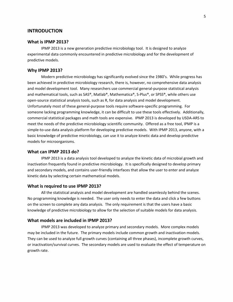
Once IPMP 2013 is initiated, an introduction screen (Figure 1) will appear. It shows the contact
information for the product. Once the introduction screen disappears, IPMP 2013 will be loaded. IPMP
2013 consists of 4 independent floating windows (Figure 2). Each window can be independently
dragged, expanded, shrunk, or closed.
Figure 1. Introduction screen (about screen).
Figure 2. Main window and its components.
7
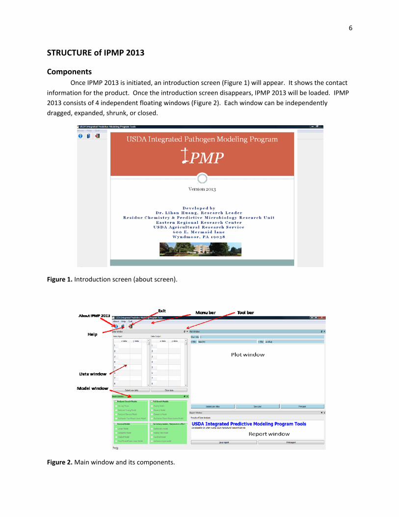
Window manipulation
To expand or shrink a window, place the cursor between two windows until appears. Drag
to expand or shrink (Figure 3). Click ‘X’ in each window to close a window. Click the double
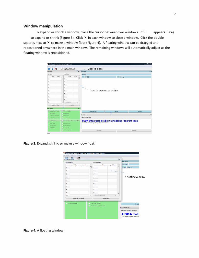
squares next to ‘X’ to make a window float (Figure 4). A floating window can be dragged and
repositioned anywhere in the main window. The remaining windows will automatically adjust as the
floating window is repositioned.
Figure 3. Expand, shrink, or make a window float.
Figure 4. A floating window.
8
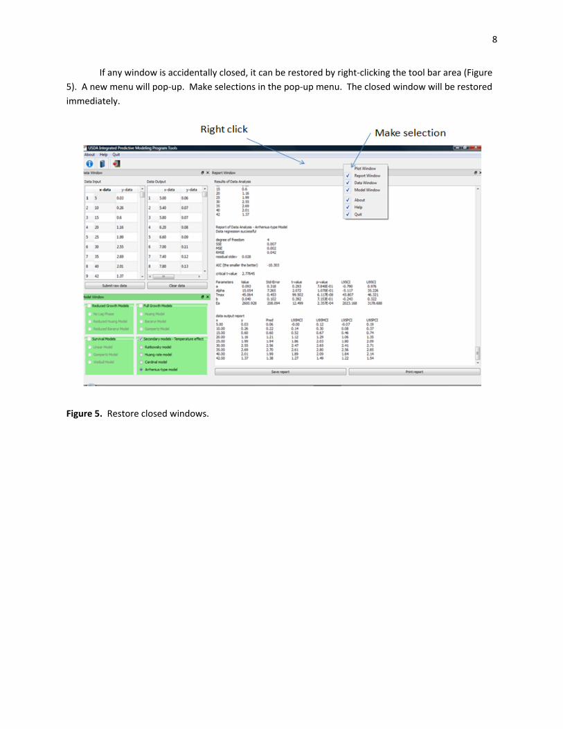
If any window is accidentally closed, it can be restored by right‐clicking the tool bar area (Figure
5). A new menu will pop‐up. Make selections in the pop‐up menu. The closed window will be restored
immediately.
Figure 5. Restore closed windows.
9
DATA WINDOW
Components
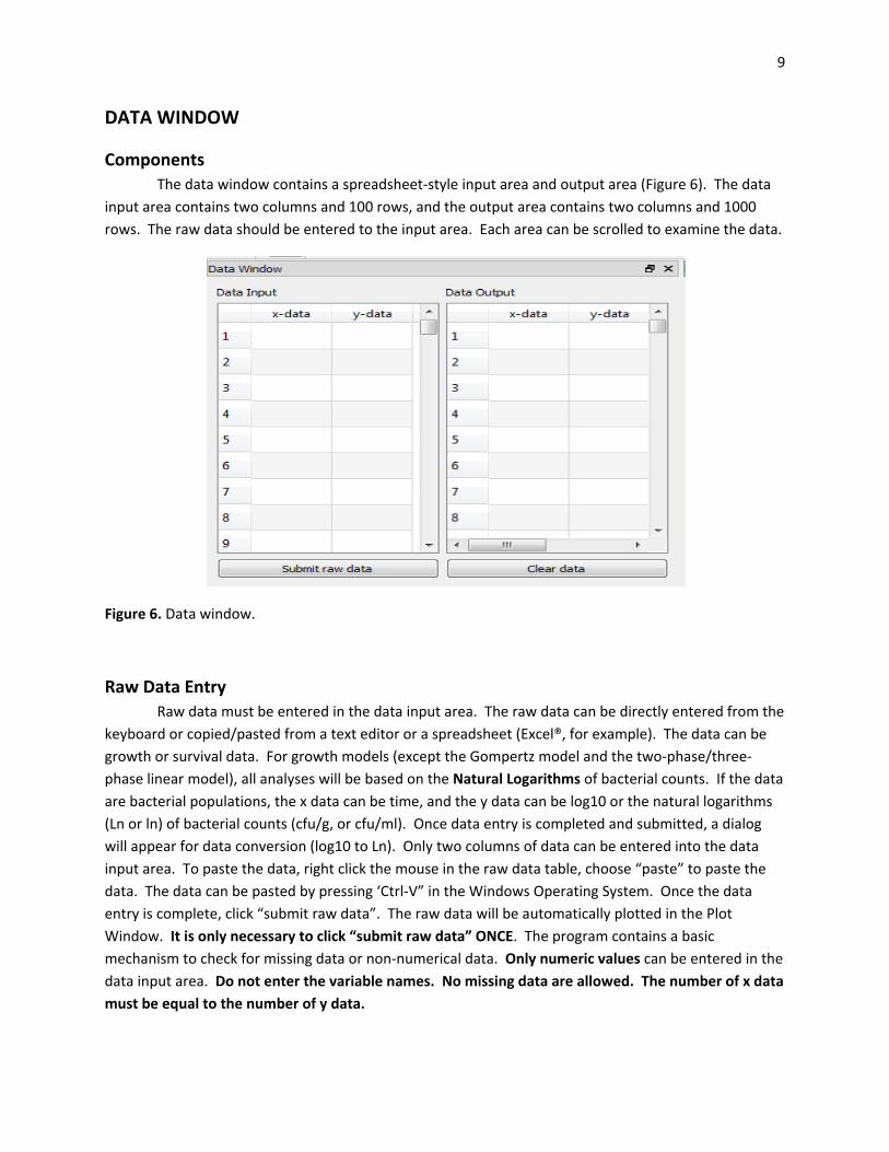
The data window contains a spreadsheet‐style input area and output area (Figure 6). The data
input area contains two columns and 100 rows, and the output area contains two columns and 1000
rows. The raw data should be entered to the input area. Each area can be scrolled to examine the data.
Figure 6. Data window.
Raw Data Entry
Raw data must be entered in the data input area. The raw data can be directly entered from the
keyboard or copied/pasted from a text editor or a spreadsheet (Excel®, for example). The data can be
growth or survival data. For growth models (except the Gompertz model and the two‐phase/three‐
phase linear model), all analyses will be based on the Natural Logarithms of bacterial counts. If the data
are bacterial populations, the x data can be time, and the y data can be log10 or the natural logarithms
(Ln or ln) of bacterial counts (cfu/g, or cfu/ml). Once data entry is completed and submitted, a dialog
will appear for data conversion (log10 to Ln). Only two columns of data can be entered into the data
input area. To paste the data, right click the mouse in the raw data table, choose “paste” to paste the
data. The data can be pasted by pressing ‘Ctrl‐V” in the Windows Operating System. Once the data
entry is complete, click “submit raw data”. The raw data will be automatically plotted in the Plot
Window. It is only necessary to click “submit raw data” ONCE. The program contains a basic
mechanism to check for missing data or non‐numerical data. Only numeric values can be entered in the
data input area. Do not enter the variable names. No missing data are allowed. The number of x data
must be equal to the number of y data.

10
Raw data can be edited by right‐clicking the mouse. The edit operations include “cut”, “copy”,
“paste”, and “clear”. The data can be saved to “cvs” format by clicking the “save” option.
If necessary, click “Clear data” to erase the data from the input area. A dialog will appear to
confirm if the data are to be cleared. Once confirmed, the data will be cleared from the memory, and
the Plot Window will be reset accordingly. Once data entry is complete, continue to Model Window for
data analysis.
Clear Raw Data
Once data analysis is complete, it is necessary to clear the data before new data can be entered,
which can be accomplished by clicking “Clear data”. Again, a dialog will appear to confirm if the data are
to be cleared. Once confirmed, the data will be cleared from the memory, and the Plot Window will be
reset accordingly.

11
MODEL WINDOW
Components and model selection
The Model Window consists of four groups of models (Figure 7). Each of them is mutually
exclusive, i.e., only one group can be selected at each time. To select a group of models, click the square
selection box next to the title of each group. Once a group is selected, the rest of the model groups will
be disabled. You have to click the square box to unselect the selected group before you can select
another group.
Figure 7. Model Window.
Adjustment of initial parameters
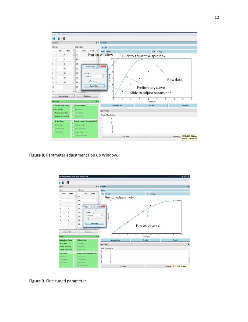
Once a group is selected, you can choose a model by clicking one of the radio buttons. Once a
model is selected, a window will pop up (Figure 8), and a preliminary curve will be plotted. The pop up
window contains the parameters for each model. Each parameter can be adjusted by adjusting the
slider or the spin box. The number of parameters depends on the model. Once a parameter is adjusted,
the preliminary curve will be automatically adjusted. Adjust the slider, spin box, or the text area to
adjust the parameter until the preliminary curve is fine‐tuned, when the preliminary curve closely
matches the raw data (Figure 9). This exercise allows nonlinear regression to converge faster. Once the
parameter(s) is fine‐tuned, click the “Submit Model” button. The data will be submitted to the data
analysis engine for processing. For linear inactivation model, no initial values window will appear.
Once data analysis is complete, the model curve will be plotted.
The data plot can be saved or printed by clicking the “Save plot” or “Print plot” button. The title
of the plot, x axis, and y‐axis can be changed by entering text in the areas above the plot. Click ‘Update
plot title” to make the changes.
12
Figure 8. Parameter adjustment Pop up Window.
Figure 9. Fine‐tuned parameter.

13
DATA REPORT WINDOW
Window components
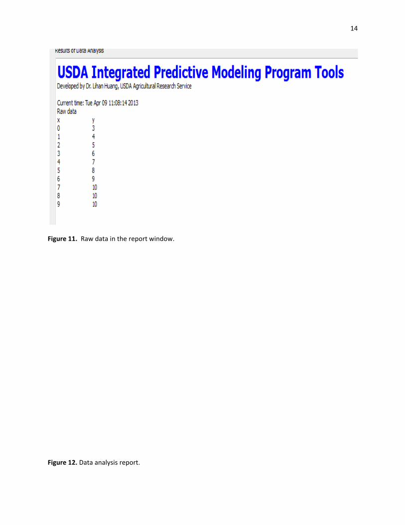
The data report window is a text reporting area to display the results of analysis (Figure 10).
Within this window, there is a button for saving the text report and another for printing. Once the data
are submitted, they will be automatically sent to the report window, along with the time when the data
are submitted (Figure 11). After the data analysis is complete, the results will also be sent to the report
window (Figure 12). The report can be saved or printed by clicking the buttons below the text area.
Figure 10. A blank data report window.
14
Figure 11. Raw data in the report window.
Figure 12. Data analysis report.

15
Data report components
n: number of data points in a curve.
p: number of parameters in a model.
df: degree of freedom, n – p.
SSE: sum of squared errors, ∑ .
MSE: mean of SSE, SSE/df.
RMSE: square root of MSE.
Residual standard deviation: standard deviation of errors.
AIC: Akaike information criterion, 2 1 , df > 2 (Brul, van Gerwen, and
Zwietering et al., 2007).
Parameters: parameters in an equation to be determined by linear or nonlinear regression.
L95CI and U95CI: lower and upper 95% confidence interval for the estimated parameters.
L95MCI and U95MCI: approximate lower and upper 95% confidence intervals for the expected value
(mean) (SAS, 2013).
L95PCI and U95PCI: approximate lower and upper 95% confidence intervals for individual prediction
(fitted value) (SAS, 2013).
16
MATHEMATICAL MODELS IN IPMP 2013
Group 1 – Reduced Growth Models
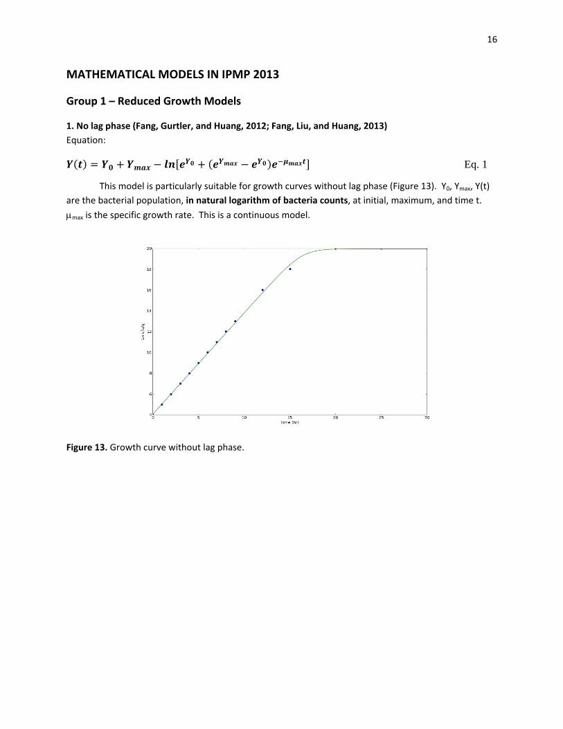
1. No lag phase (Fang, Gurtler, and Huang, 2012; Fang, Liu, and Huang, 2013)
Equation:
Eq. 1
This model is particularly suitable for growth curves without lag phase (Figure 13). Y0, Ymax, Y(t)
are the bacterial population, in natural logarithm of bacteria counts, at initial, maximum, and time t.
max is the specific growth rate. This is a continuous model.
Figure 13. Growth curve without lag phase.
17
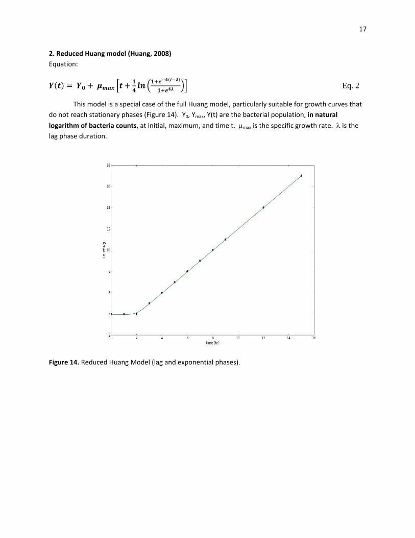
2. Reduced Huang model (Huang, 2008)
Equation:
Eq. 2
This model is a special case of the full Huang model, particularly suitable for growth curves that
do not reach stationary phases (Figure 14). Y0, Ymax, Y(t) are the bacterial population, in natural
logarithm of bacteria counts, at initial, maximum, and time t. max is the specific growth rate. is the lag phase duration.
Figure 14. Reduced Huang Model (lag and exponential phases).
18
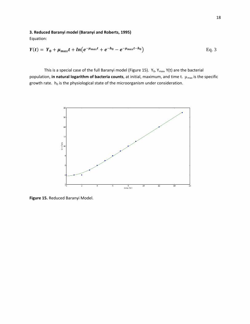
3. Reduced Baranyi model (Baranyi and Roberts, 1995)
Equation:
Eq. 3
This is a special case of the full Baranyi model (Figure 15). Y0, Ymax, Y(t) are the bacterial
population, in natural logarithm of bacteria counts, at initial, maximum, and time t. max is the specific
growth rate. h0 is the physiological state of the microorganism under consideration.
Figure 15. Reduced Baranyi Model.
19
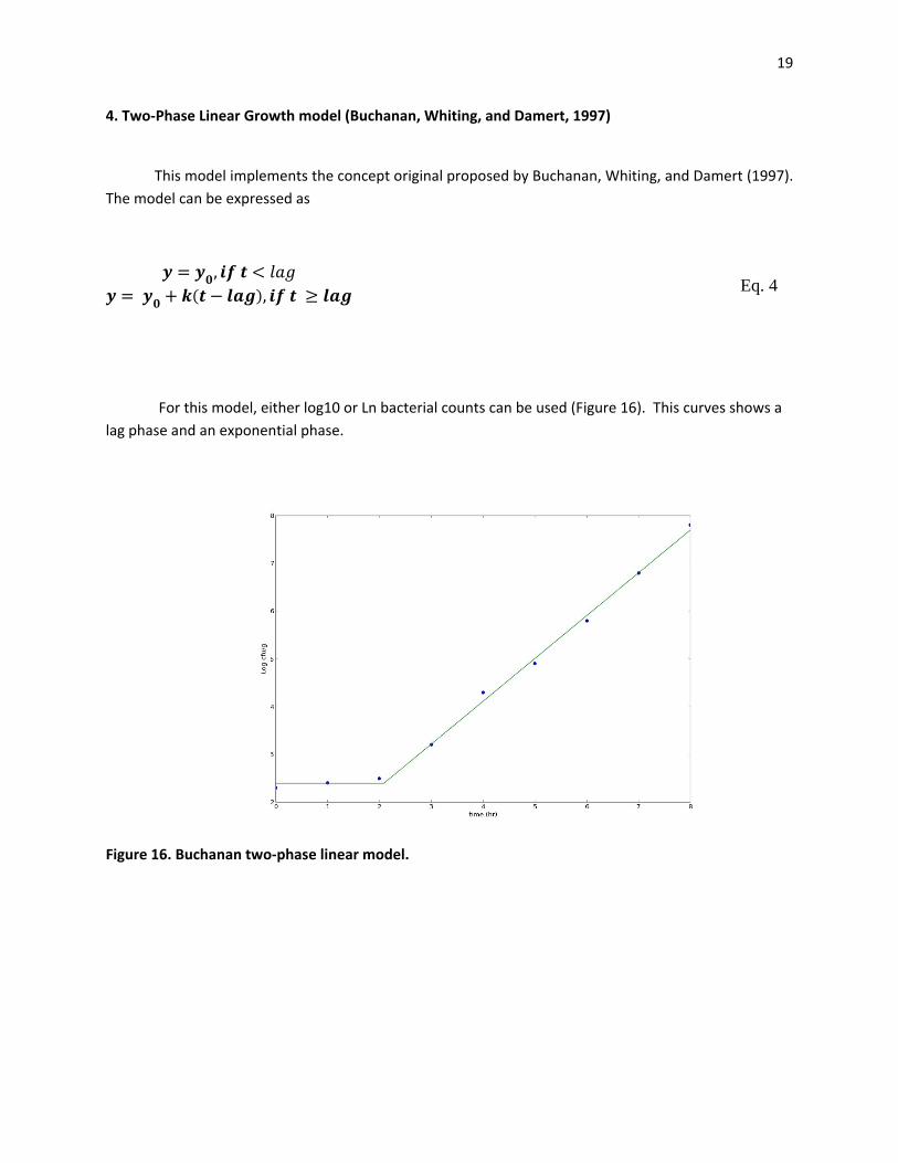
4. Two‐Phase Linear Growth model (Buchanan, Whiting, and Damert, 1997)
This model implements the concept original proposed by Buchanan, Whiting, and Damert (1997).
The model can be expressed as
, , Eq. 4
For this model, either log10 or Ln bacterial counts can be used (Figure 16). This curves shows a
lag phase and an exponential phase.
Figure 16. Buchanan two‐phase linear model.
20
Group 2. Full growth Models
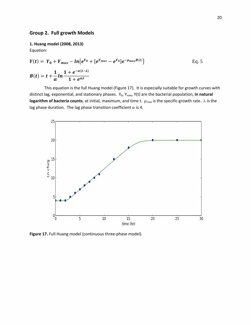
1. Huang model (2008, 2013)
Equation:
Eq. 5
This equation is the full Huang model (Figure 17). It is especially suitable for growth curves with
distinct lag, exponential, and stationary phases. Y0, Ymax, Y(t) are the bacterial population, in natural
logarithm of bacteria counts, at initial, maximum, and time t. max is the specific growth rate. is the lag phase duration. The lag phase transition coefficient is 4.
Figure 17. Full Huang model (continuous three‐phase model).
21
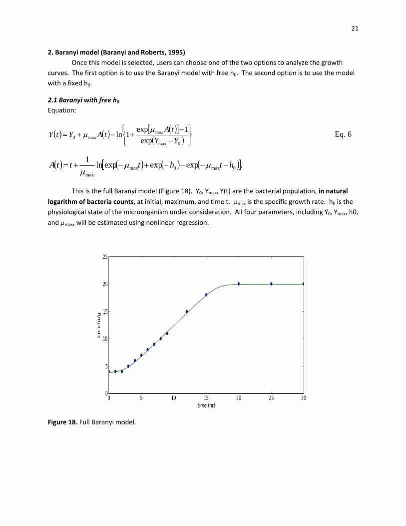
2. Baranyi model (Baranyi and Roberts, 1995)
Once this model is selected, users can choose one of the two options to analyze the growth
curves. The first option is to use the Baranyi model with free h0. The second option is to use the model
with a fixed h0.
2.1 Baranyi with free h0
Equation:
0max
maxmax0 exp
1exp1ln
YY
tAtAYtY
Eq. 6
.expexpexpln1
0max0maxmax
hthtttA
This is the full Baranyi model (Figure 18). Y0, Ymax, Y(t) are the bacterial population, in natural
logarithm of bacteria counts, at initial, maximum, and time t. max is the specific growth rate. h0 is the
physiological state of the microorganism under consideration. All four parameters, including Y0, Ymax, h0,
and max, will be estimated using nonlinear regression.
Figure 18. Full Baranyi model.
22
2.2 Baranyi model with a fixed h0
The application of the Baranyi model usually involves two steps. In the first step, each growth
curve is analyzed using the Baranyi model to determine h0 and max. Afert all the growth curves are
analyzed, an average of h0 is then calculated. Using this averaged h0, each growth curve is reanalyzed to
obtain a new value of max. The new values of max are used to generate a secondary model. With h0
fixed, the AIC value is inherently smaller.
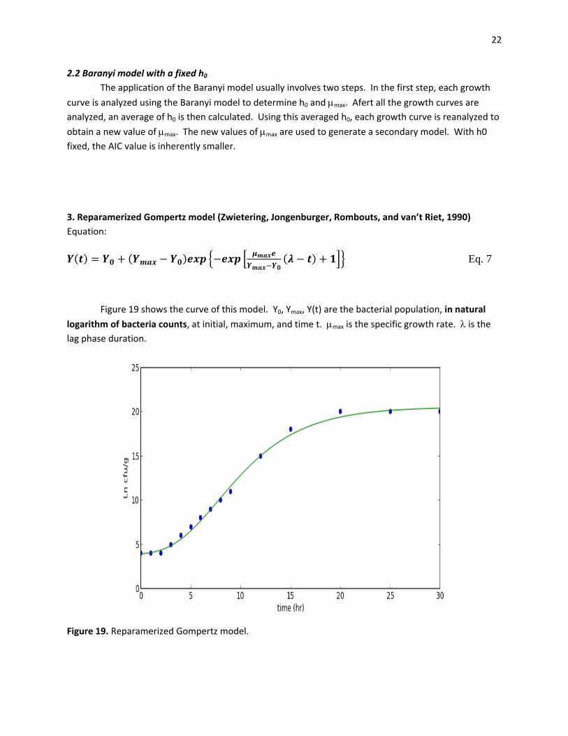
3. Reparamerized Gompertz model (Zwietering, Jongenburger, Rombouts, and van’t Riet, 1990)
Equation:
Eq. 7
Figure 19 shows the curve of this model. Y0, Ymax, Y(t) are the bacterial population, in natural
logarithm of bacteria counts, at initial, maximum, and time t. max is the specific growth rate. is the lag phase duration.
Figure 19. Reparamerized Gompertz model.
23
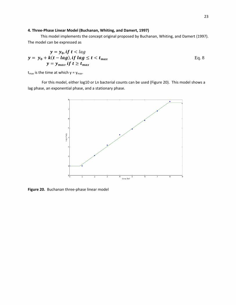
4. Three‐Phase Linear Model (Buchanan, Whiting, and Damert, 1997)
This model implements the concept original proposed by Buchanan, Whiting, and Damert (1997).
The model can be expressed as
, ,
, Eq. 8
tmax is the time at which y = ymax.
For this model, either log10 or Ln bacterial counts can be used (Figure 20). This model shows a
lag phase, an exponential phase, and a stationary phase.
Figure 20. Buchanan three‐phase linear model
24
Group 3. Survival Models
1. Linear model
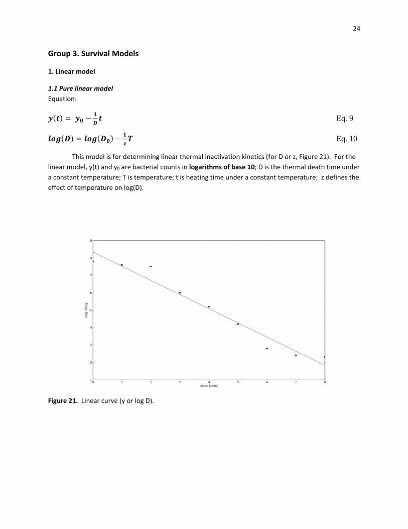
1.1 Pure linear model
Equation:
Eq. 9
Eq. 10
This model is for determining linear thermal inactivation kinetics (for D or z, Figure 21). For the
linear model, y(t) and y0 are bacterial counts in logarithms of base 10; D is the thermal death time under
a constant temperature; T is temperature; t is heating time under a constant temperature; z defines the
effect of temperature on log(D).
Figure 21. Linear curve (y or log D).
25
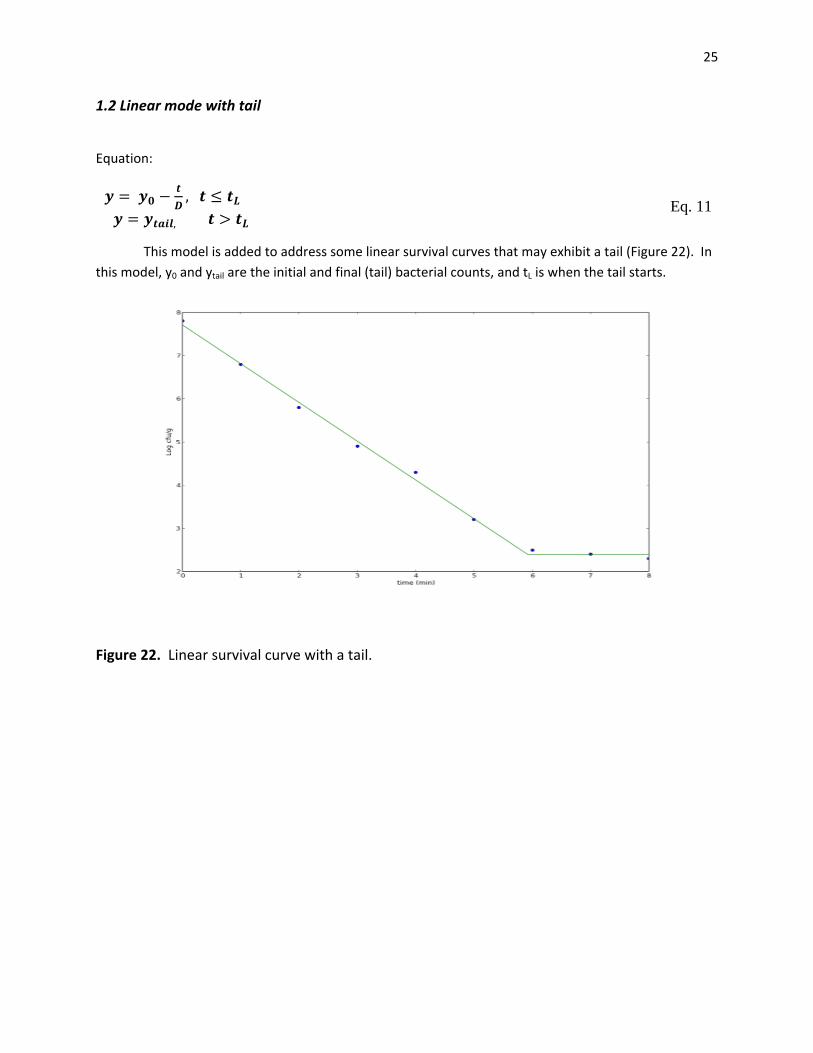
1.2 Linear mode with tail
Equation:
, ,
Eq. 11
This model is added to address some linear survival curves that may exhibit a tail (Figure 22). In
this model, y0 and ytail are the initial and final (tail) bacterial counts, and tL is when the tail starts.
Figure 22. Linear survival curve with a tail.
26
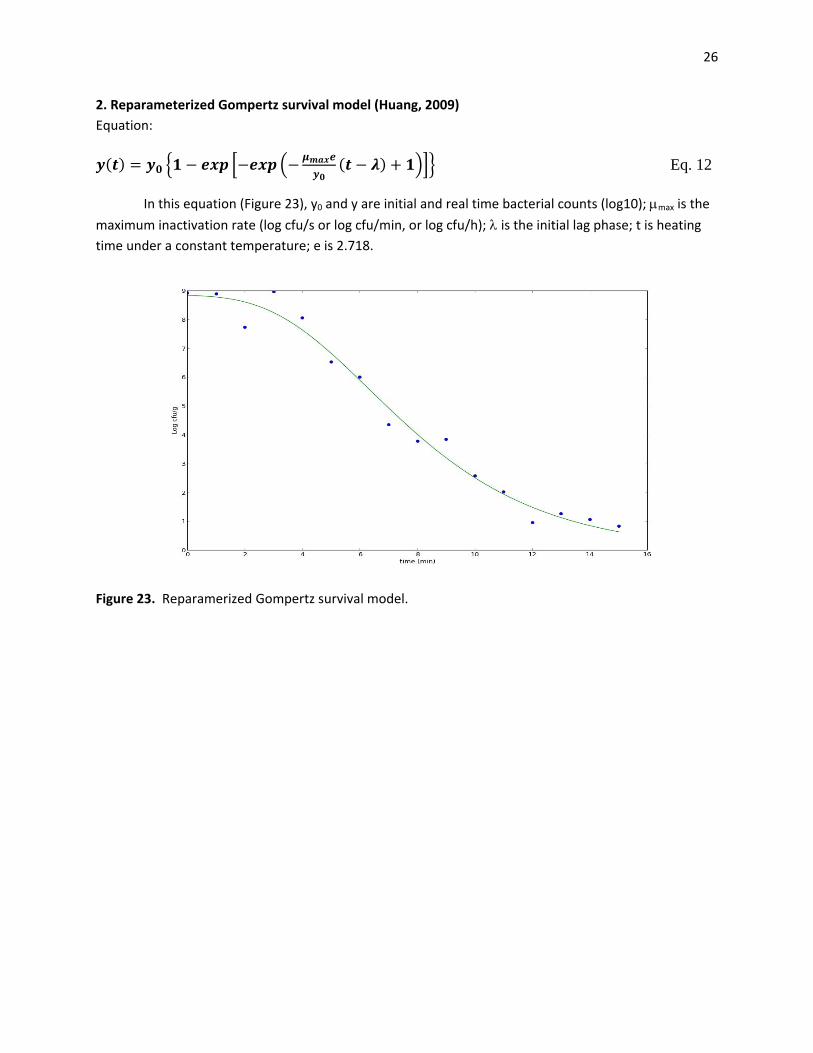
2. Reparameterized Gompertz survival model (Huang, 2009)
Equation:
Eq. 12
In this equation (Figure 23), y0 and y are initial and real time bacterial counts (log10); max is the
maximum inactivation rate (log cfu/s or log cfu/min, or log cfu/h); is the initial lag phase; t is heating time under a constant temperature; e is 2.718.
Figure 23. Reparamerized Gompertz survival model.
27
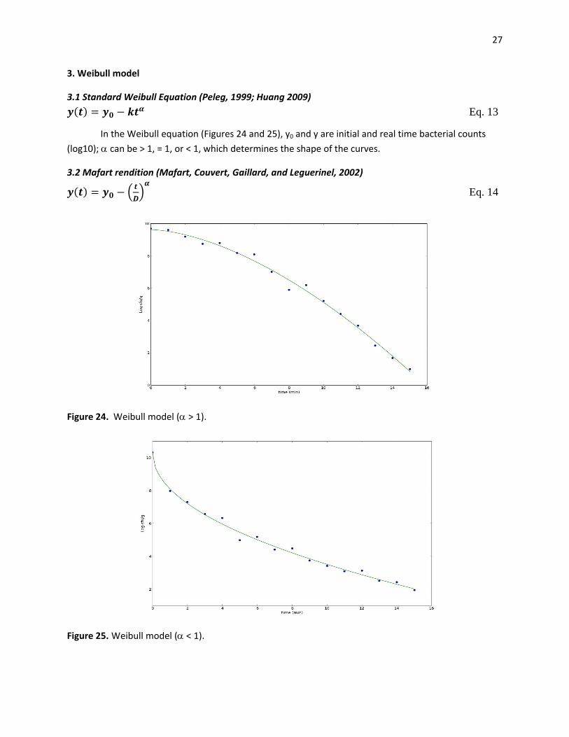
3. Weibull model
3.1 Standard Weibull Equation (Peleg, 1999; Huang 2009)
Eq. 13
In the Weibull equation (Figures 24 and 25), y0 and y are initial and real time bacterial counts
(log10); can be > 1, = 1, or < 1, which determines the shape of the curves.
3.2 Mafart rendition (Mafart, Couvert, Gaillard, and Leguerinel, 2002)
Eq. 14
Figure 24. Weibull model ( > 1).
Figure 25. Weibull model ( < 1).
28
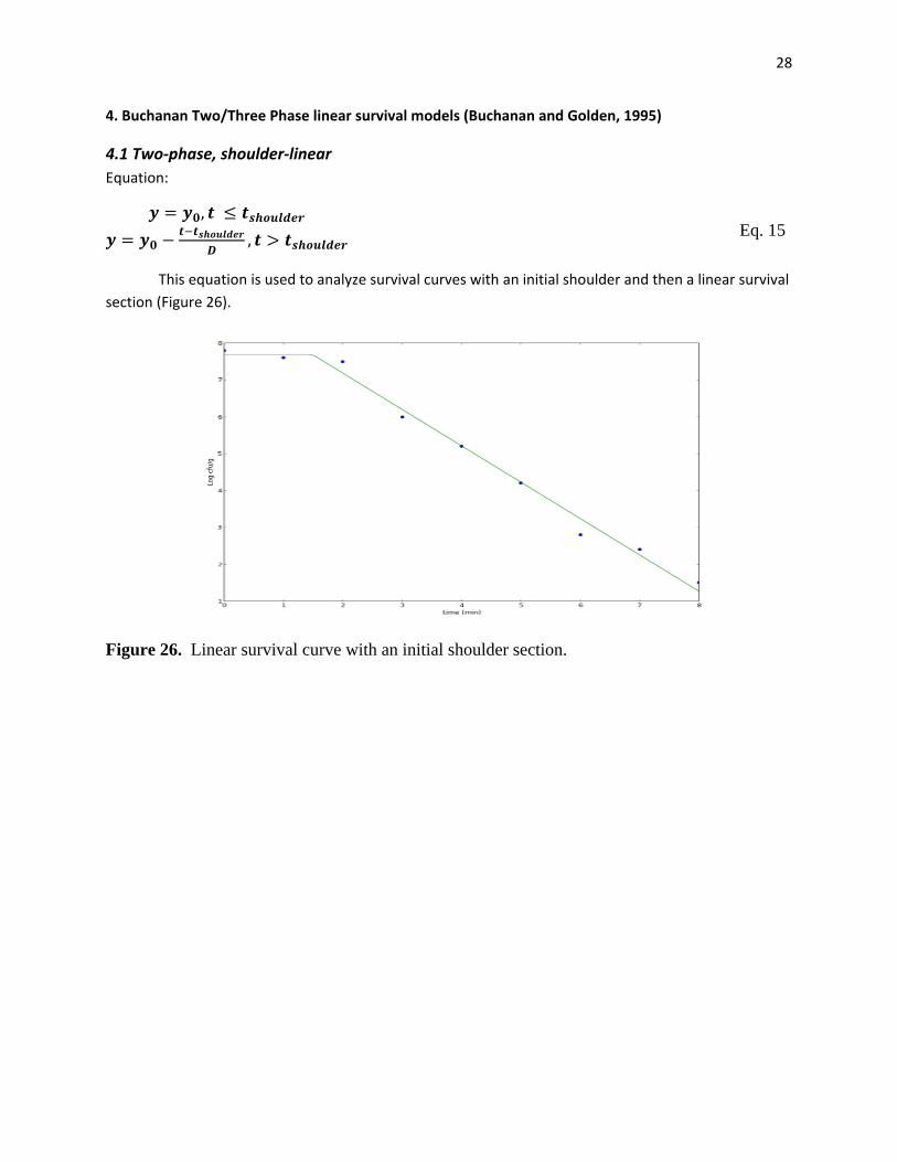
4. Buchanan Two/Three Phase linear survival models (Buchanan and Golden, 1995)
4.1 Two‐phase, shoulder‐linear
Equation:
,
, Eq. 15
This equation is used to analyze survival curves with an initial shoulder and then a linear survival
section (Figure 26).
Figure 26. Linear survival curve with an initial shoulder section.
29
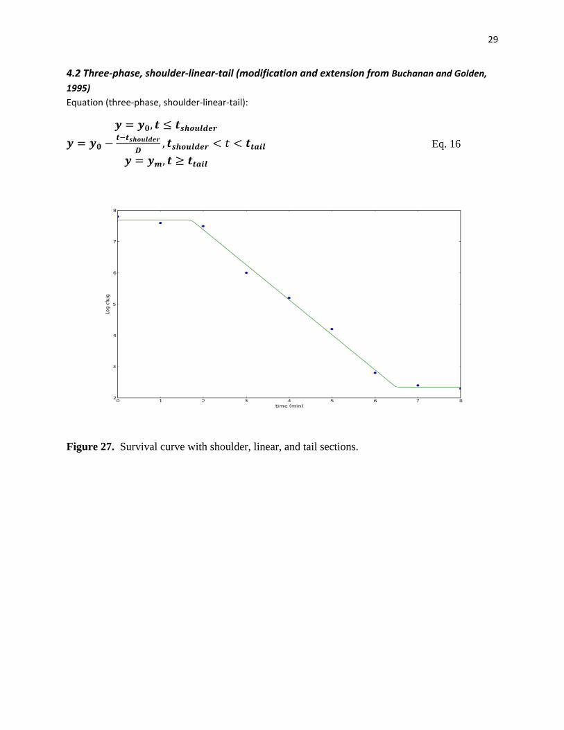
4.2 Three‐phase, shoulder‐linear‐tail (modification and extension from Buchanan and Golden,
1995)
Equation (three‐phase, shoulder‐linear‐tail):
,
,,
Eq. 16
Figure 27. Survival curve with shoulder, linear, and tail sections.
30
Group 4. Secondary models – effect of temperature on growth rate
1. Ratkowsky square‐root model
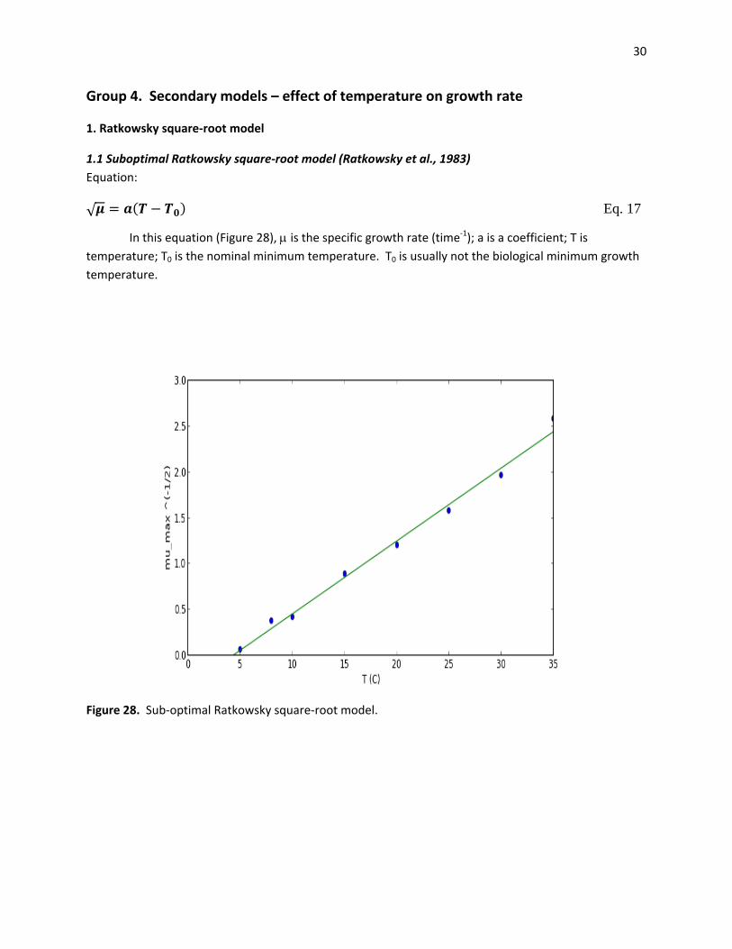
1.1 Suboptimal Ratkowsky square‐root model (Ratkowsky et al., 1983)
Equation:
√ Eq. 17
In this equation (Figure 28), is the specific growth rate (time‐1); a is a coefficient; T is
temperature; T0 is the nominal minimum temperature. T0 is usually not the biological minimum growth
temperature.
Figure 28. Sub‐optimal Ratkowsky square‐root model.
31
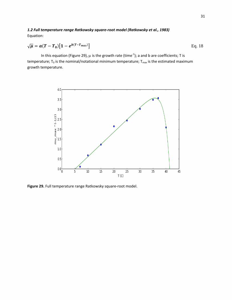
1.2 Full temperature range Ratkowsky square‐root model (Ratkowsky et al., 1983)
Equation:
√ Eq. 18
In this equation (Figure 29), is the growth rate (time‐1); a and b are coefficients; T is
temperature; T0 is the nominal/notational minimum temperature; Tmax is the estimated maximum
growth temperature.
Figure 29. Full temperature range Ratkowsky square‐root model.
32
2. Huang square‐root model
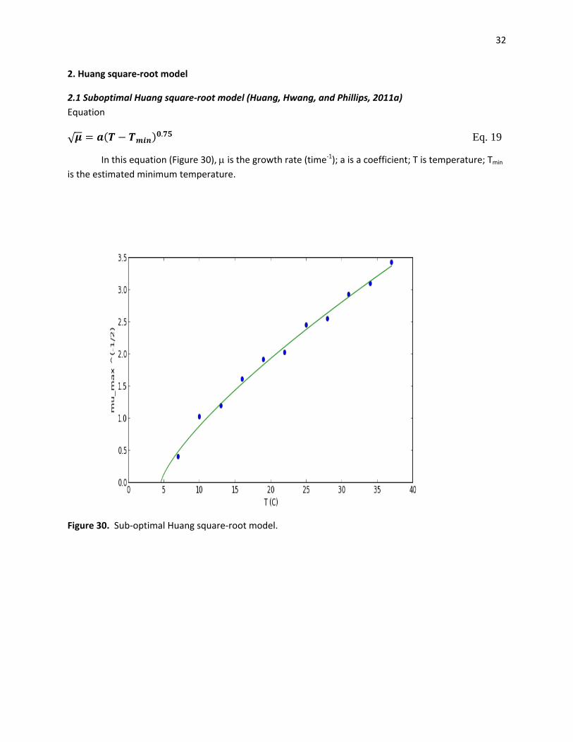
2.1 Suboptimal Huang square‐root model (Huang, Hwang, and Phillips, 2011a)
Equation
√ . Eq. 19
In this equation (Figure 30), is the growth rate (time‐1); a is a coefficient; T is temperature; Tmin
is the estimated minimum temperature.
Figure 30. Sub‐optimal Huang square‐root model.
33
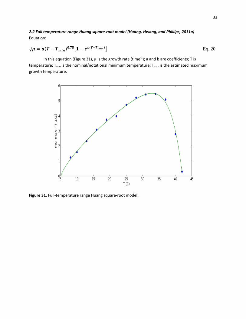
2.2 Full temperature range Huang square‐root model (Huang, Hwang, and Phillips, 2011a)
Equation:
√ . Eq. 20
In this equation (Figure 31), is the growth rate (time‐1); a and b are coefficients; T is
temperature; Tmin is the nominal/notational minimum temperature; Tmax is the estimated maximum
growth temperature.
Figure 31. Full‐temperature range Huang square‐root model.
34
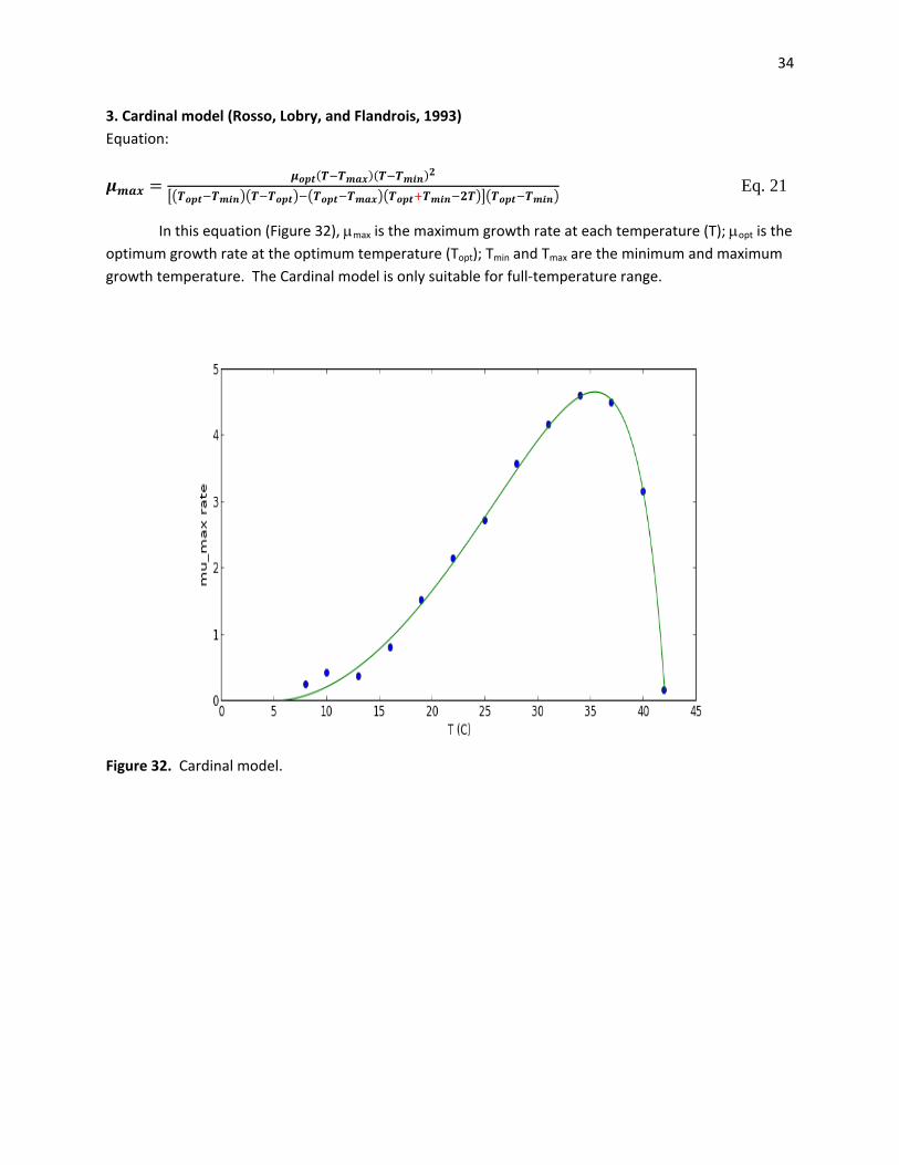
3. Cardinal model (Rosso, Lobry, and Flandrois, 1993)
Equation:
Eq. 21
In this equation (Figure 32), max is the maximum growth rate at each temperature (T); opt is the
optimum growth rate at the optimum temperature (Topt); Tmin and Tmax are the minimum and maximum
growth temperature. The Cardinal model is only suitable for full‐temperature range.
Figure 32. Cardinal model.
35
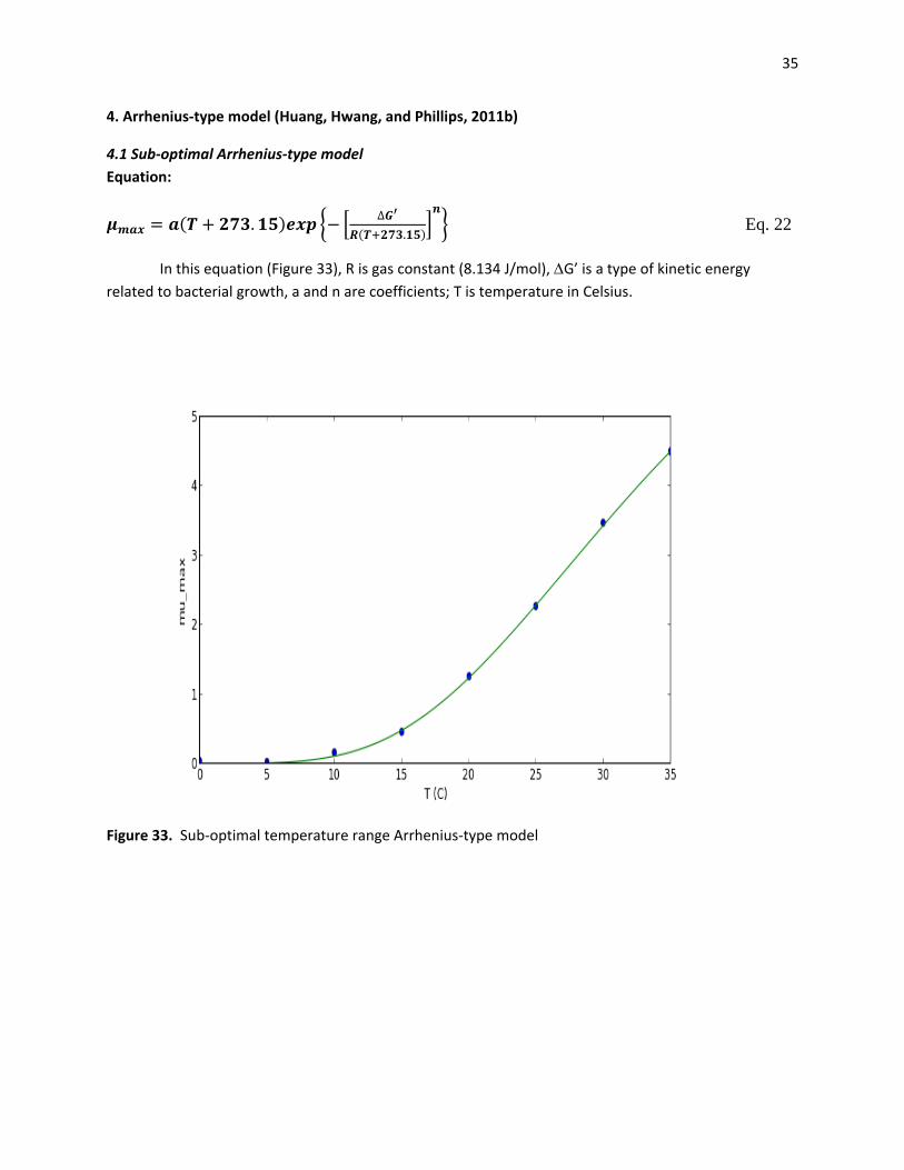
4. Arrhenius‐type model (Huang, Hwang, and Phillips, 2011b)
4.1 Sub‐optimal Arrhenius‐type model
Equation:
. ∆
. Eq. 22
In this equation (Figure 33), R is gas constant (8.134 J/mol), G’ is a type of kinetic energy related to bacterial growth, a and n are coefficients; T is temperature in Celsius.
Figure 33. Sub‐optimal temperature range Arrhenius‐type model
36
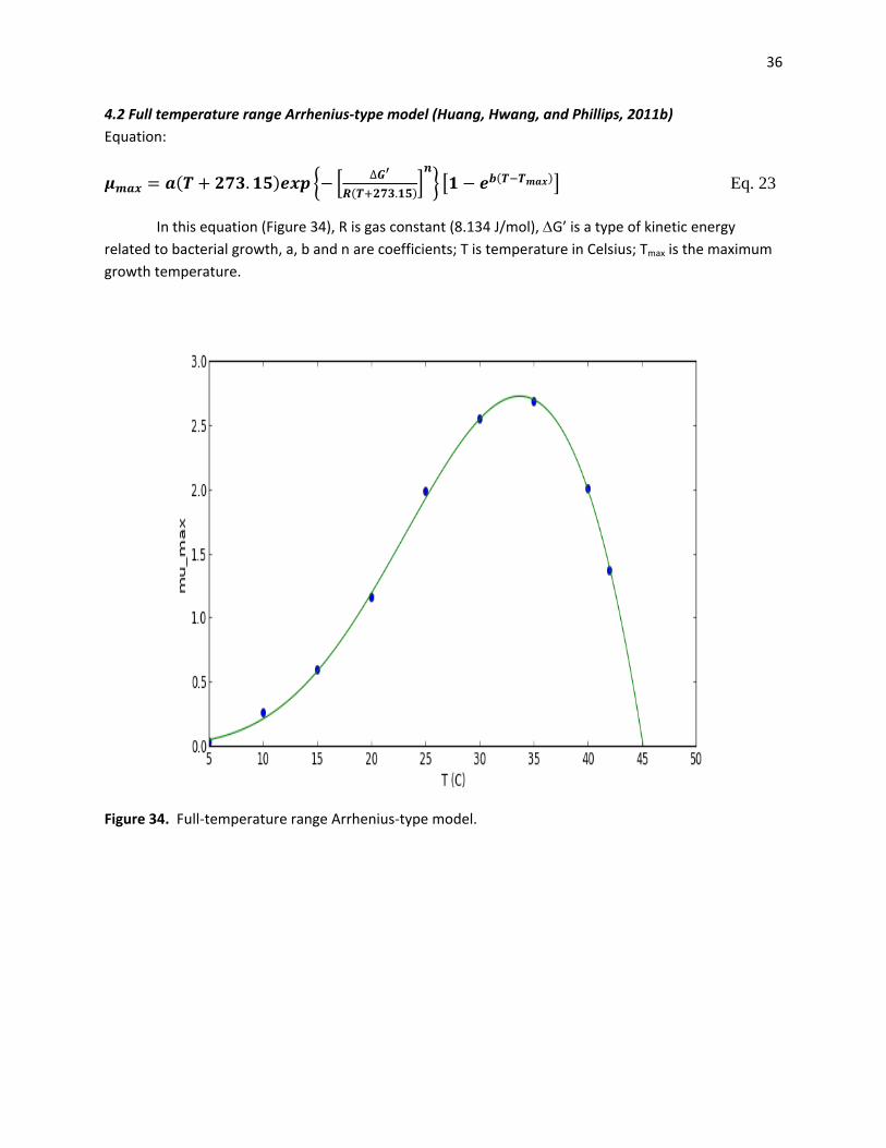
4.2 Full temperature range Arrhenius‐type model (Huang, Hwang, and Phillips, 2011b)
Equation:
. ∆
. Eq. 23
In this equation (Figure 34), R is gas constant (8.134 J/mol), G’ is a type of kinetic energy related to bacterial growth, a, b and n are coefficients; T is temperature in Celsius; Tmax is the maximum
growth temperature.
Figure 34. Full‐temperature range Arrhenius‐type model.
37
References Baranyi, J. and Roberts, T.A. 1995. Mathematics of predictive microbiology. International Journal of
Food Microbiology, 26, 199 – 218.
Brul, S., van Gerwen, S., and Zwietering, M. 2007. Modeling microorganisms in food. Woodhead
Publishing Limited, Cambridge, UK, and CRC Press, Boca Raton, FL.
Buchanan, R. and Golden, M. 1995. Model for the non‐thermal inactivation of Liseria monocytogenes in
a reduced oxygen environment. Food Microbiology, 12, 230 – 212.
Buchanan, R. L., Whiting, R. C., and Damert, W. C. 1997. When is simple good enough: a comparison of
the Gompertz, Baranyi, and three‐phase linear models for fitting bacterial growth curves. Food
Microbiology, 14, 313 – 326.
Fang, T., Gurtler, J.B., and Huang, L. 2012. Growth kinetics and model comparison of Cronobacter
sakazakii in reconstituted powdered infant formula. Journal of Food Science, 77, E247 – E255.
Fang, T., Liu, Y., and Huang, L. 2013. Growth kinetics of Listeria monocytogenes and spoilage
microorganisms in fresh‐cut cantaloupe. Food Microbiology, 34, 174 – 181.
Huang, L. 2008. Growth kinetics of Listeria monocytogenes in broth and beef frankfurters –
determination of lag phase duration and exponential growth rate under isothermal conditions. Journal
of Food Science, 73, E235 – 242.
Huang, L. 2009. Thermal inactivation of Listeria monocytogenes in ground beef under isothermal and
dynamic temperature conditions. Journal of Food Engineering, 90, 380 – 387.
Huang, L., Hwang, C., and Phillips, J.G. 2011a. Evaluating the effect of temperature on microbial growth
rate ‐ the Ratkowsky and a Belehrádek type models. Journal of Food Science, 76, M547‐557.
Huang, L., Hwang, C., and Phillips, J.G. 2011b. Effect of temperature on microbial growth rate ‐
thermodynamic analysis, the Arrhenius and Eyring‐Polanyi connection. Journal of Food Science, 76,
E553‐560.
Huang, L. 2013. Optimization of a new mathematical model for bacterial growth. Food Control, 32, 283
– 288.
Mafart, P., Couvert, O., Gaillard, S., and Leguerinel. 2002. On calculating sterility in thermal
preservation methods: application of the Weibull frequency distribution model. International Journal of
Food Microbiology, 72: 107 – 113.
Peleg, M. 1999. On calculating sterility in thermal and non‐thermal preservation methods. Food
Research International, 32: 271 – 278.
Rosso, L., Lobry, J.R., and Flandrois, J.P. 1993. An unexpected correlation between cardinal temperatures
of microbial growth highlighted by a new model. Journal of Theoretical Biology 162:447–63.

38
Ratkowsky, D,A., Lowry, R.K., McMeekin, T.A., Stokes, A.N., and Chandler, R.E. 1983. Model for bacterial
culture growth rate through the entire biokinetic temperature range. Journal of Bacteriology 154: 1222–
6.
SAS. 2013. SAS/STAT® 9.22 User’s Guide, The NLIN Procedure. SAS Institute, Cary, NC.
Zwietering, M.H., Jongenburger, I., Rombouts, F.M., and van’t Riet, K. 1990. Modeling of the bacterial
growth curve. Applied and Environmental Microbiology, 56, 1875 – 1881.