Embed Size (px)
Citation preview
.
......
Introduction to Inter-universal Teichmuller
Theory II
— An Etale Aspect of the Theory of Etale Theta Functions —
Yuichiro Hoshi
RIMS, Kyoto University
December 2, 2015
Yuichiro Hoshi (RIMS, Kyoto University) Introduction to IUT II December 2, 2015 1 / 26
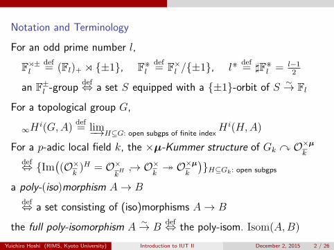
Notation and Terminology
For an odd prime number l,
F⋊±l
def= (Fl)+ ⋊ {±1}, F⋇
l
def= F×
l /{±1}, l⋇def= ♯F⋇
l = l−12
an F±l -group
def⇔ a set S equipped with a {±1}-orbit of S ∼→ Fl
For a topological group G,
∞H i(G,A)def= lim−→H⊆G: open subgps of finite index
H i(H,A)
For a p-adic local field k, the ×µ-Kummer structure of Gk ↷ O×µ
kdef⇔ {Im
((O×
k)H = O×
kH ↪→ O×
k↠ O×µ
k
)}H⊆Gk: open subgps
a poly-(iso)morphism A→ Bdef⇔ a set consisting of (iso)morphisms A→ B
the full poly-isomorphism A∼→ B
def⇔ the poly-isom. Isom(A,B)
Yuichiro Hoshi (RIMS, Kyoto University) Introduction to IUT II December 2, 2015 2 / 26
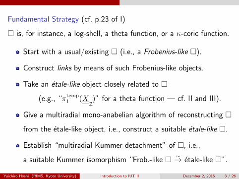
Fundamental Strategy (cf. p.23 of I)
□ is, for instance, a log-shell, a theta function, or a κ-coric function.
Start with a usual/existing □ (i.e., a Frobenius-like □).
Construct links by means of such Frobenius-like objects.
Take an etale-like object closely related to □(e.g., “πtemp
1 (Xv)” for a theta function — cf. II and III).
Give a multiradial mono-anabelian algorithm of reconstructing □from the etale-like object, i.e., construct a suitable etale-like □.
Establish “multiradial Kummer-detachment” of □, i.e.,
a suitable Kummer isomorphism “Frob.-like □ ∼→ etale-like □”.
Yuichiro Hoshi (RIMS, Kyoto University) Introduction to IUT II December 2, 2015 3 / 26
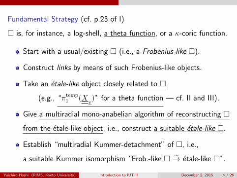
Fundamental Strategy (cf. p.23 of I)
□ is, for instance, a log-shell, a theta function, or a κ-coric function.
Start with a usual/existing □ (i.e., a Frobenius-like □).
Construct links by means of such Frobenius-like objects.
Take an etale-like object closely related to □(e.g., “πtemp
1 (Xv)” for a theta function — cf. II and III).
Give a multiradial mono-anabelian algorithm of reconstructing □from the etale-like object, i.e., construct a suitable etale-like □.
Establish “multiradial Kummer-detachment” of □, i.e.,
a suitable Kummer isomorphism “Frob.-like □ ∼→ etale-like □”.
Yuichiro Hoshi (RIMS, Kyoto University) Introduction to IUT II December 2, 2015 4 / 26
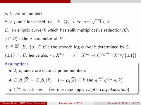
p, l: prime numbers
k: a p-adic local field, i.e., [k : Qp] <∞, s.t.√−1 ∈ k
E: an elliptic curve/k which has split multiplicative reduction/Ok
q ∈ O▷k : the q-parameter of E
X log def= (E, {o} ⊆ E): the smooth log curve/k determined by E
{±1}↷ E, hence also ↷ X log ⇒ X log → C log def= [X log/{±1}]
.Assumptions..
......
2, p, and l are distinct prime numbers
E[2l](k) = E[2l](k) (⇔ µl(k) ⊆ k and qdef= q1/2l ∈ k)
C log is a k-core (⇒ one may apply elliptic cuspidalization)
Yuichiro Hoshi (RIMS, Kyoto University) Introduction to IUT II December 2, 2015 5 / 26
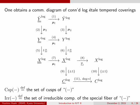
One obtains a comm. diagram of conn’d log etale tempered coverings
Ylog (1)−−−→
µl
Y log
(2)
yµ2 (3)
yµ2
Y log (4)−−−→µl
Y log
(5)
yl·Z (6)
yl·Z
X log (7)−−−→µl
X log (8)−−−→Fl
X log
(9)
y{±1} (10)
y{±1}
C log (11), deg=l−−−−−−→ C log
Csp(−) def= the set of cusps of “(−)”
Irr(−) def= the set of irreducible comp. of the special fiber of “(−)”
Yuichiro Hoshi (RIMS, Kyoto University) Introduction to IUT II December 2, 2015 6 / 26
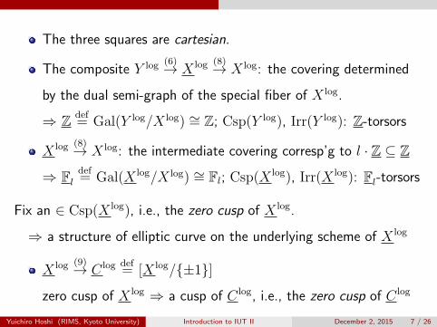
The three squares are cartesian.
The composite Y log (6)→ X log (8)→ X log: the covering determined
by the dual semi-graph of the special fiber of X log.
⇒ Z def= Gal(Y log/X log) ∼= Z; Csp(Y log), Irr(Y log): Z-torsors
X log (8)→ X log: the intermediate covering corresp’g to l · Z ⊆ Z
⇒ Fldef= Gal(X log/X log) ∼= Fl; Csp(X
log), Irr(X log): Fl-torsors
Fix an ∈ Csp(X log), i.e., the zero cusp of X log.
⇒ a structure of elliptic curve on the underlying scheme of X log
X log (9)→ C log def= [X log/{±1}]
zero cusp of X log ⇒ a cusp of C log, i.e., the zero cusp of C log
Yuichiro Hoshi (RIMS, Kyoto University) Introduction to IUT II December 2, 2015 7 / 26
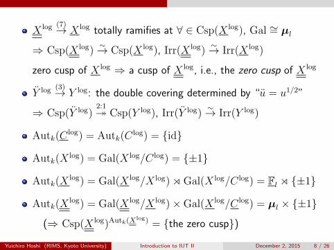
X log (7)→ X log totally ramifies at ∀ ∈ Csp(X log), Gal ∼= µl
⇒ Csp(X log)∼→ Csp(X log), Irr(X log)
∼→ Irr(X log)
zero cusp of X log ⇒ a cusp of X log, i.e., the zero cusp of X log
Y log (3)→ Y log: the double covering determined by “u = u1/2”
⇒ Csp(Y log)2:1↠ Csp(Y log), Irr(Y log)
∼→ Irr(Y log)
Autk(Clog) = Autk(C
log) = {id}
Autk(Xlog) = Gal(X log/C log) = {±1}
Autk(Xlog) = Gal(X log/X log)⋊Gal(X log/C log) = Fl ⋊ {±1}
Autk(Xlog) = Gal(X log/X log)×Gal(X log/C log) = µl × {±1}
(⇒ Csp(X log)Autk(Xlog) = {the zero cusp})
Yuichiro Hoshi (RIMS, Kyoto University) Introduction to IUT II December 2, 2015 8 / 26
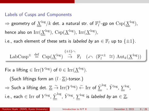
Labels of Cusps and Components
⇒ geometry of X log/k det. a natural str. of F±l -gp on Csp(X log),
hence also on Irr(X log), Csp(X log), Irr(X log),
i.e., each element of these sets is labeled by an ∈ Fl up to {±1}..
...... LabCusp± def= Csp(X log)
{±1}↷∼→ Fl (↶ (F⋊±
l∼=) Autk(X
log))
Fix a lifting ∈ Irr(Y log) of 0 ∈ Irr(X log).
(Such liftings form an (l · Z)-torsor.)
⇒ Such a lifting det. Z ∼→ Irr(Y log)∼← Irr of Y
log, Y log, Y log,
i.e., each ∈ Irr of Y log, Ylog, Y log, Y log is labeled by an ∈ Z.
Yuichiro Hoshi (RIMS, Kyoto University) Introduction to IUT II December 2, 2015 9 / 26
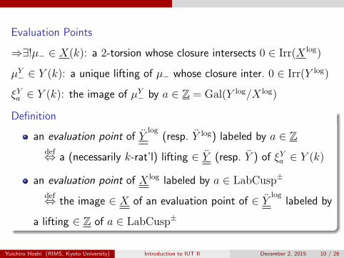
Evaluation Points
⇒∃!µ− ∈ X(k): a 2-torsion whose closure intersects 0 ∈ Irr(X log)
µY− ∈ Y (k): a unique lifting of µ− whose closure inter. 0 ∈ Irr(Y log)
ξYa ∈ Y (k): the image of µY− by a ∈ Z = Gal(Y log/X log)
.Definition..
......
an evaluation point of Ylog
(resp. Y log) labeled by a ∈ Zdef⇔ a (necessarily k-rat’l) lifting ∈ Y (resp. Y ) of ξYa ∈ Y (k)
an evaluation point of X log labeled by a ∈ LabCusp±
def⇔ the image ∈ X of an evaluation point of ∈ Ylog
labeled by
a lifting ∈ Z of a ∈ LabCusp±
Yuichiro Hoshi (RIMS, Kyoto University) Introduction to IUT II December 2, 2015 10 / 26
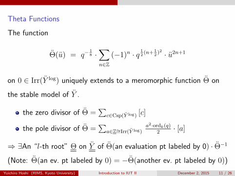
Theta Functions
The function
Θ(u) = q−18 ·
∑n∈Z
(−1)n · q12(n+ 1
2)2 · u2n+1
on 0 ∈ Irr(Y log) uniquely extends to a meromorphic function Θ on
the stable model of Y .
the zero divisor of Θ =∑
c∈Csp(Y log) [c]
the pole divisor of Θ =∑
a∈Z∼=Irr(Y log)a2·ordk(q)
2· [a]
⇒ ∃An “l-th root” Θ on Y of Θ(an evaluation pt labeled by 0) · Θ−1
(Note: Θ(an ev. pt labeled by 0) = −Θ(another ev. pt labeled by 0))
Yuichiro Hoshi (RIMS, Kyoto University) Introduction to IUT II December 2, 2015 11 / 26
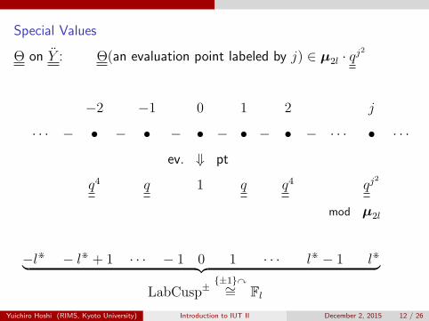
Special Values
Θ on Y : Θ(an evaluation point labeled by j) ∈ µ2l · qj2
−2 −1 0 1 2 j
· · · − • − • − • − • − • − · · · • · · ·
ev. ⇓ pt
q4 q 1 q q4 qj2
mod µ2l
−l⋇ − l⋇ + 1 · · · − 1 0 1 · · · l⋇ − 1 l⋇︸ ︷︷ ︸LabCusp±
{±1}↷∼= Fl
Yuichiro Hoshi (RIMS, Kyoto University) Introduction to IUT II December 2, 2015 12 / 26
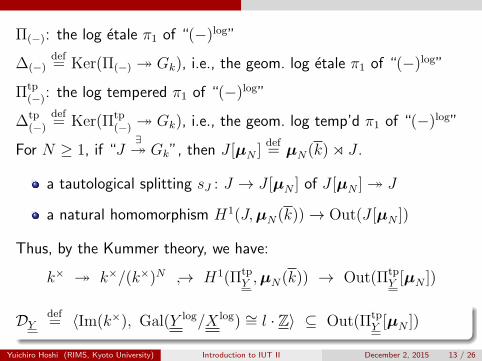
Π(−): the log etale π1 of “(−)log”
∆(−)def= Ker(Π(−) ↠ Gk), i.e., the geom. log etale π1 of “(−)log”
Πtp(−): the log tempered π1 of “(−)log”
∆tp(−)
def= Ker(Πtp
(−) ↠ Gk), i.e., the geom. log temp’d π1 of “(−)log”
For N ≥ 1, if “J∃↠ Gk”, then J [µN ]
def= µN(k)⋊ J .
a tautological splitting sJ : J → J [µN ] of J [µN ] ↠ J
a natural homomorphism H1(J,µN(k))→ Out(J [µN ])
Thus, by the Kummer theory, we have:
k× ↠ k×/(k×)N ↪→ H1(ΠtpY ,µN(k)) → Out(Πtp
Y [µN ])
.
......DY
def= ⟨Im(k×), Gal(Y log/X log) ∼= l · Z⟩ ⊆ Out(Πtp
Y [µN ])
Yuichiro Hoshi (RIMS, Kyoto University) Introduction to IUT II December 2, 2015 13 / 26
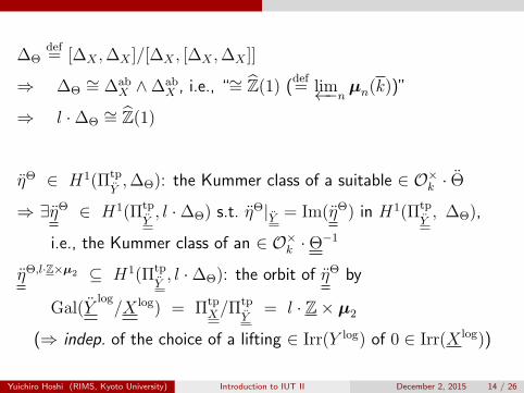
∆Θdef= [∆X ,∆X ]/[∆X , [∆X ,∆X ]]
⇒ ∆Θ∼= ∆ab
X ∧∆abX , i.e., “∼= Z(1) (def= lim←−n
µn(k))”
⇒ l ·∆Θ∼= Z(1)
ηΘ ∈ H1(Πtp
Y,∆Θ): the Kummer class of a suitable ∈ O×
k · Θ
⇒ ∃ηΘ ∈ H1(Πtp
Y, l ·∆Θ) s.t. η
Θ|Y = Im(ηΘ) in H1(Πtp
Y, ∆Θ),
i.e., the Kummer class of an ∈ O×k ·Θ
−1
ηΘ,l·Z×µ2 ⊆ H1(Πtp
Y, l ·∆Θ): the orbit of ηΘ by
Gal(Ylog/X log) = Πtp
X/Πtp
Y= l · Z× µ2
(⇒ indep. of the choice of a lifting ∈ Irr(Y log) of 0 ∈ Irr(X log))
Yuichiro Hoshi (RIMS, Kyoto University) Introduction to IUT II December 2, 2015 14 / 26
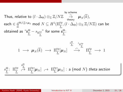
Thus, relative to (l ·∆Θ)⊗Z Z/NZby scheme
∼→theory
µN(k),
each ∈ ηΘ,l·Z×µ2 mod N ⊆ H1(Πtp
Y, (l ·∆Θ)⊗Z Z/NZ) can be
obtained as “sΘY− sΠtp
Y
” for some sΘY:
1 −→ µN(k) −→ Πtp
Y[µN ]
sΘY
, sΠtp
Y↶−→ Πtp
Y−→ 1
.
......sΘY: Πtp
Y
sΘY
↪→ Πtp
Y[µN ] ↪→ Πtp
Y [µN ] : a (mod N) theta section
Yuichiro Hoshi (RIMS, Kyoto University) Introduction to IUT II December 2, 2015 15 / 26
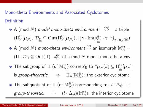
Mono-theta Environments and Associated Cyclotomes.Definition..
......
A (mod N) model mono-theta environmentdef⇔ a triple
(ΠtpY [µN ], DY ⊆ Out(Πtp
Y [µN ]), {γ · Im(sΘY) · γ−1}γ∈µN (k))
A (mod N) mono-theta environmentdef⇔ an isomorph MΘ
N =
(Π, DΠ ⊆ Out(Π), sΘΠ) of a mod N model mono-theta env.
The subgroup of Π (of MΘN) corresp’g to “µN(k) ⊆ Πtp
Y [µN ]”
is group-theoretic. ⇒ Πµ(MΘN): the exterior cyclotome
The subquotient of Π (of MΘN) corresponding to “l ·∆Θ” is
group-theoretic. ⇒ (l ·∆Θ)(MΘN): the interior cyclotome
Yuichiro Hoshi (RIMS, Kyoto University) Introduction to IUT II December 2, 2015 16 / 26
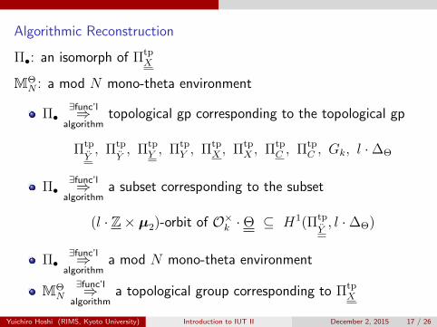
Algorithmic Reconstruction
Π•: an isomorph of ΠtpX
MΘN : a mod N mono-theta environment
Π•∃func’l⇒
algorithmtopological gp corresponding to the topological gp
Πtp
Y, Πtp
Y, Πtp
Y , ΠtpY , Πtp
X , ΠtpX , Πtp
C , ΠtpC , Gk, l ·∆Θ
Π•∃func’l⇒
algorithma subset corresponding to the subset
(l · Z× µ2)-orbit of O×k ·Θ ⊆ H1(Πtp
Y, l ·∆Θ)
Π•∃func’l⇒
algorithma mod N mono-theta environment
MΘN
∃func’l⇒algorithm
a topological group corresponding to ΠtpX
Yuichiro Hoshi (RIMS, Kyoto University) Introduction to IUT II December 2, 2015 17 / 26
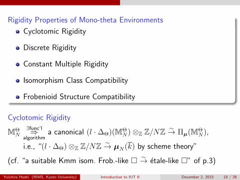
.Rigidity Properties of Mono-theta Environments..
......
Cyclotomic Rigidity
Discrete Rigidity
Constant Multiple Rigidity
Isomorphism Class Compatibility
Frobenioid Structure Compatibility
Cyclotomic Rigidity
MΘN
∃func’l⇒algorithm
a canonical (l ·∆Θ)(MΘN)⊗Z Z/NZ ∼→ Πµ(MΘ
N),
i.e., “(l ·∆Θ)⊗Z Z/NZ ∼→ µN(k) by scheme theory”
(cf. “a suitable Kmm isom. Frob.-like □ ∼→ etale-like □” of p.3)
Yuichiro Hoshi (RIMS, Kyoto University) Introduction to IUT II December 2, 2015 18 / 26
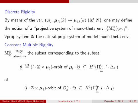
Discrete Rigidity
By means of the var. surj. µN(k) ↠ µM(k) (M |N), one may define
the notion of a “projective system of mono-theta env. {MΘN}N≥1”.
∀proj. system ∼= the natural proj. system of model mono-theta env.
Constant Multiple Rigidity
MΘN
∃func’l⇒algorithm
the subset corresponding to the subset
θdef= (l · Z× µ2)-orbit of µl ·Θ ⊆ H1(Πtp
Y, l ·∆Θ)
of
(l · Z× µ2)-orbit of O×k ·Θ ⊆ H1(Πtp
Y, l ·∆Θ)
Yuichiro Hoshi (RIMS, Kyoto University) Introduction to IUT II December 2, 2015 19 / 26
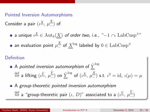
Pointed Inversion Automorphisms
Consider a pair (ιX , µX
− ) of
a unique ιX ∈ Autk(X) of order two, i.e., “−1 ↷ LabCusp±”
an evaluation point µX
− of X log labeled by 0 ∈ LabCusp±
.Definition..
......
A pointed inversion automorphism of Ylog
def⇔ a lifting (ιY , µY
−) on Ylog
of (ιX , µX
− ) s.t. ι2 = id, ι(µ) = µ
A group-theoretic pointed inversion automorphismdef⇔ a “group-theoretic pair (ι, D)” associated to a (ιY , µ
Y
−)
Yuichiro Hoshi (RIMS, Kyoto University) Introduction to IUT II December 2, 2015 20 / 26
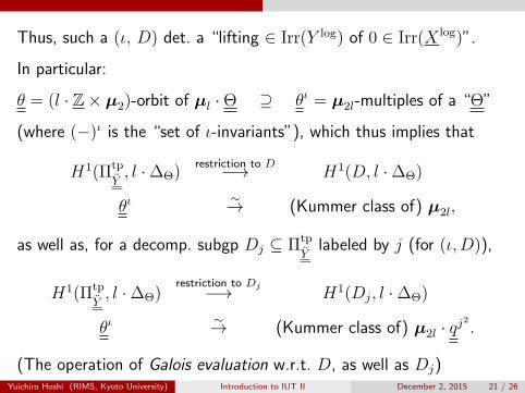
Thus, such a (ι, D) det. a “lifting ∈ Irr(Y log) of 0 ∈ Irr(X log)”.
In particular:
θ = (l · Z× µ2)-orbit of µl ·Θ ⊇ θι = µ2l-multiples of a “Θ”
(where (−)ι is the “set of ι-invariants”), which thus implies that
H1(Πtp
Y, l ·∆Θ)
restriction to D−→ H1(D, l ·∆Θ)
θι∼→ (Kummer class of) µ2l,
as well as, for a decomp. subgp Dj ⊆ Πtp
Ylabeled by j (for (ι,D)),
H1(Πtp
Y, l ·∆Θ)
restriction to Dj−→ H1(Dj, l ·∆Θ)
θι∼→ (Kummer class of) µ2l · qj
2.
(The operation of Galois evaluation w.r.t. D, as well as Dj)Yuichiro Hoshi (RIMS, Kyoto University) Introduction to IUT II December 2, 2015 21 / 26
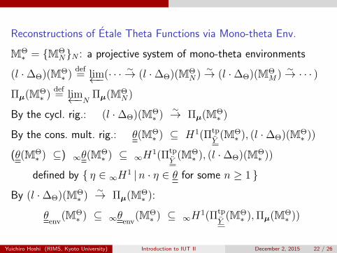
Reconstructions of Etale Theta Functions via Mono-theta Env.
MΘ∗ = {MΘ
N}N : a projective system of mono-theta environments
(l ·∆Θ)(MΘ∗ )
def= lim←−(· · ·
∼→ (l ·∆Θ)(MΘN)
∼→ (l ·∆Θ)(MΘM)
∼→ · · · )
Πµ(MΘ∗ )
def= lim←−N
Πµ(MΘN)
By the cycl. rig.: (l ·∆Θ)(MΘ∗ )
∼→ Πµ(MΘ∗ )
By the cons. mult. rig.: θ(MΘ∗ ) ⊆ H1(Πtp
Y(MΘ
∗ ), (l ·∆Θ)(MΘ∗ ))
(θ(MΘ∗ ) ⊆) ∞θ(MΘ
∗ ) ⊆ ∞H1(Πtp
Y(MΘ
∗ ), (l ·∆Θ)(MΘ∗ ))
defined by { η ∈ ∞H1 |n · η ∈ θ for some n ≥ 1 }
By (l ·∆Θ)(MΘ∗ )
∼→ Πµ(MΘ∗ ):
θenv
(MΘ∗ ) ⊆ ∞θ
env(MΘ
∗ ) ⊆ ∞H1(Πtp
Y(MΘ
∗ ),Πµ(MΘ∗ ))
Yuichiro Hoshi (RIMS, Kyoto University) Introduction to IUT II December 2, 2015 22 / 26
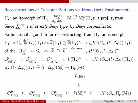
Reconstructions of Constant Portions via Mono-theta Environments
Π•: an isomorph of ΠtpX
func’l⇒algorithm
M def= MΘ
∗ (Π•): a proj. system
Since X log is of strictly Belyi type, by Belyi cuspidalization,
∃a functorial algorithm for reconstructing, from Π•, an isomorph
Π• ↠ G•def= Gk(Π•) ↷ k(Π•) ⊇ k(Π•)
× ↪→ ∞H1(G•, (l ·∆Θ)(Π•))
of the “ΠtpX ↠ Gk ↷ k ⊇ k
× Kummer↪→ ∞H1(Gk, l ·∆Θ)”
Oµ
k(Π•)⊆ O×
k(Π•)⊆ O▷
k(Π•)⊆ k(Π•)
× ⊆ ∞H1(G•, (l ·∆Θ)(Π•))
By (l ·∆Θ)(Π•)∼→ (l ·∆Θ)(M)
∼→ Πµ(M):
k(M)
∪
Oµ
k(M)⊆ O×
k(M)⊆ O▷
k(M)⊆ k(M)× ⊆ ∞H1(G•,Πµ(M))
Yuichiro Hoshi (RIMS, Kyoto University) Introduction to IUT II December 2, 2015 23 / 26
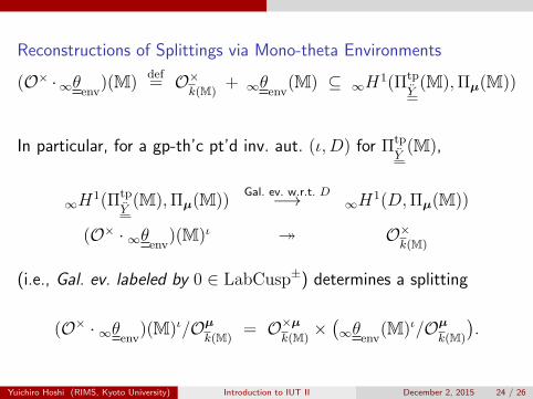
Reconstructions of Splittings via Mono-theta Environments
(O× ·∞θenv
)(M)def= O×
k(M)+ ∞θ
env(M) ⊆ ∞H1(Πtp
Y(M),Πµ(M))
In particular, for a gp-th’c pt’d inv. aut. (ι,D) for Πtp
Y(M),
∞H1(Πtp
Y(M),Πµ(M))
Gal. ev. w.r.t. D−→ ∞H1(D,Πµ(M))
(O× · ∞θenv
)(M)ι ↠ O×k(M)
(i.e., Gal. ev. labeled by 0 ∈ LabCusp±) determines a splitting
(O× · ∞θenv
)(M)ι/Oµ
k(M)= O×µ
k(M)×
(∞θ
env(M)ι/Oµ
k(M)
).
Yuichiro Hoshi (RIMS, Kyoto University) Introduction to IUT II December 2, 2015 24 / 26
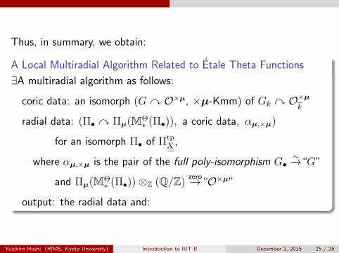
Thus, in summary, we obtain:.A Local Multiradial Algorithm Related to Etale Theta Functions..
......
∃A multiradial algorithm as follows:
coric data: an isomorph (G ↷ O×µ, ×µ-Kmm) of Gk ↷ O×µ
k
radial data: (Π• ↷ Πµ(MΘ∗ (Π•)), a coric data, αµ,×µ)
for an isomorph Π• of ΠtpX ,
where αµ,×µ is the pair of the full poly-isomorphism G•∼→“G”
and Πµ(MΘ∗ (Π•))⊗Z (Q/Z) zero→“O×µ”
output: the radial data and:
Yuichiro Hoshi (RIMS, Kyoto University) Introduction to IUT II December 2, 2015 25 / 26
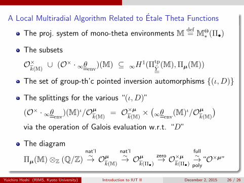
.A Local Multiradial Algorithm Related to Etale Theta Functions..
......
The proj. system of mono-theta environments M def= MΘ
∗ (Π•)
The subsets
O×k(M)
∪ (O× · ∞θenv
)(M) ⊆ ∞H1(Πtp
Y(M),Πµ(M))
The set of group-th’c pointed inversion automorphisms {(ι,D)}
The splittings for the various “(ι,D)”
(O× · ∞θenv
)(M)ι/Oµ
k(M)= O×µ
k(M)×
(∞θ
env(M)ι/Oµ
k(M)
)via the operation of Galois evaluation w.r.t. “D”
The diagram
Πµ(M)⊗Z (Q/Z)nat’l∼→ Oµ
k(M)
nat’l∼→ Oµ
k(Π•)
zero→ O×µ
k(Π•)
full∼→
poly“O×µ”
Yuichiro Hoshi (RIMS, Kyoto University) Introduction to IUT II December 2, 2015 26 / 26


![ABELIAN ETALE COVERINGS OF GENERIC CURVES´ AND ORDINARINESS OF DORMANT … · 2018. 9. 22. · arXiv:1602.07061v1 [math.AG] 23 Feb 2016 ABELIAN ETALE COVERINGS OF GENERIC CURVES´](https://img.pdfslide.net/doc/110x75/602d323b6884d4157b3c6126/abelian-etale-coverings-of-generic-curves-and-ordinariness-of-dormant-2018-9.jpg)