Embed Size (px)
Citation preview
Introduction to Machine Learning (67577)Lecture 10
Shai Shalev-Shwartz
School of CS and Engineering,The Hebrew University of Jerusalem
Neural Networks
Shai Shalev-Shwartz (Hebrew U) IML Lecture 10 Neural Networks 1 / 31

Outline
1 Neural networks
2 Sample Complexity
3 Expressiveness of neural networks
4 How to train neural networks ?Computational hardnessSGDBack-Propagation
5 Convolutional Neural Networks (CNN)
6 Feature Learning
Shai Shalev-Shwartz (Hebrew U) IML Lecture 10 Neural Networks 2 / 31

A Single Artificial Neuron
A single neuron is a function of the form x 7→ σ(〈v,x〉), whereσ : R→ R is called the activation function of the neuron
x1
x2
x3
x4
x5
σ(〈v, x〉)
v1
v2
v3
v4
v5
E.g., σ is a sigmoidal function
Shai Shalev-Shwartz (Hebrew U) IML Lecture 10 Neural Networks 3 / 31

Neural Networks
A neural network is obtained by connecting many neurons together
We focus on feedforward networks, formally defined by a directedacyclic graph G = (V,E)
Input nodes: nodes with no incoming edges
Output nodes: nodes without out going edges
weights: w : E → RCalculation using breadth-first-search (BFS), where each neuron(node) receives as input:
a[v] =∑
u→v∈Ew[u→ v]o[u]
and outputo[v] = σ(a[v])
Shai Shalev-Shwartz (Hebrew U) IML Lecture 10 Neural Networks 4 / 31

Neural Networks
A neural network is obtained by connecting many neurons together
We focus on feedforward networks, formally defined by a directedacyclic graph G = (V,E)
Input nodes: nodes with no incoming edges
Output nodes: nodes without out going edges
weights: w : E → R
Calculation using breadth-first-search (BFS), where each neuron(node) receives as input:
a[v] =∑
u→v∈Ew[u→ v]o[u]
and outputo[v] = σ(a[v])
Shai Shalev-Shwartz (Hebrew U) IML Lecture 10 Neural Networks 4 / 31

Neural Networks
A neural network is obtained by connecting many neurons together
We focus on feedforward networks, formally defined by a directedacyclic graph G = (V,E)
Input nodes: nodes with no incoming edges
Output nodes: nodes without out going edges
weights: w : E → RCalculation using breadth-first-search (BFS), where each neuron(node) receives as input:
a[v] =∑
u→v∈Ew[u→ v]o[u]
and outputo[v] = σ(a[v])
Shai Shalev-Shwartz (Hebrew U) IML Lecture 10 Neural Networks 4 / 31

Multilayer Neural Networks
Neurons are organized in layers: V = ·∪Tt=0Vt, and edges are onlybetween adjacent layersExample of a multilayer neural network of depth 3 and size 6
x1
x2
x3
x4
x5
Hiddenlayer
Hiddenlayer
Inputlayer
Outputlayer
Shai Shalev-Shwartz (Hebrew U) IML Lecture 10 Neural Networks 5 / 31

Neural Networks as a Hypothesis Class
Given a neural network (V,E, σ, w), we obtain a hypothesishV,E,σ,w : R|V0|−1 → R|VT |
We refer to (V,E, σ) as the architecture, and it defines a hypothesisclass by
HV,E,σ = hV,E,σ,w : w is a mapping from E to R .
The architecture is our “Prior knowledge” and the learning task is tofind the weight function w
We can now studyestimation error (sample complexity)approximation error (expressivenss)optimization error (computational complexity)
Shai Shalev-Shwartz (Hebrew U) IML Lecture 10 Neural Networks 6 / 31

Outline
1 Neural networks
2 Sample Complexity
3 Expressiveness of neural networks
4 How to train neural networks ?Computational hardnessSGDBack-Propagation
5 Convolutional Neural Networks (CNN)
6 Feature Learning
Shai Shalev-Shwartz (Hebrew U) IML Lecture 10 Neural Networks 7 / 31

Sample Complexity
Theorem: The VC dimension of HV,E,sign is O(|E| log(|E|)).
Theorem: The VC dimension of HV,E,σ, for σ being the sigmoidalfunction, is Ω(|E|2).
Representation trick: In practice, we only care about networks whereeach weight is represented using O(1) bits, and therefore the VCdimension of such networks is O(|E|), no matter what σ is
We can further decrease the sample complexity by many kinds ofregularization functions (this is left for an advanced course)
Shai Shalev-Shwartz (Hebrew U) IML Lecture 10 Neural Networks 8 / 31

Outline
1 Neural networks
2 Sample Complexity
3 Expressiveness of neural networks
4 How to train neural networks ?Computational hardnessSGDBack-Propagation
5 Convolutional Neural Networks (CNN)
6 Feature Learning
Shai Shalev-Shwartz (Hebrew U) IML Lecture 10 Neural Networks 9 / 31

What can we express with neural networks ?
For simplicity, lets focus on boolean inputs and sign activationfunctions.
What type of functions from ±1n to ±1 can be implemented byHV,E,sign ?
Theorem: For every n, there exists a graph (V,E) of depth 2, suchthat HV,E,sign contains all functions from ±1n to ±1Theorem: For every n, let s(n) be the minimal integer such thatthere exists a graph (V,E) with |V | = s(n) such that the hypothesisclass HV,E,sign contains all the functions from 0, 1n to 0, 1.Then, s(n) is exponential in n.
What type of functions can be implemented by networks of small size?
Shai Shalev-Shwartz (Hebrew U) IML Lecture 10 Neural Networks 10 / 31

What can we express with neural networks ?
For simplicity, lets focus on boolean inputs and sign activationfunctions.
What type of functions from ±1n to ±1 can be implemented byHV,E,sign ?
Theorem: For every n, there exists a graph (V,E) of depth 2, suchthat HV,E,sign contains all functions from ±1n to ±1
Theorem: For every n, let s(n) be the minimal integer such thatthere exists a graph (V,E) with |V | = s(n) such that the hypothesisclass HV,E,sign contains all the functions from 0, 1n to 0, 1.Then, s(n) is exponential in n.
What type of functions can be implemented by networks of small size?
Shai Shalev-Shwartz (Hebrew U) IML Lecture 10 Neural Networks 10 / 31

What can we express with neural networks ?
For simplicity, lets focus on boolean inputs and sign activationfunctions.
What type of functions from ±1n to ±1 can be implemented byHV,E,sign ?
Theorem: For every n, there exists a graph (V,E) of depth 2, suchthat HV,E,sign contains all functions from ±1n to ±1Theorem: For every n, let s(n) be the minimal integer such thatthere exists a graph (V,E) with |V | = s(n) such that the hypothesisclass HV,E,sign contains all the functions from 0, 1n to 0, 1.Then, s(n) is exponential in n.
What type of functions can be implemented by networks of small size?
Shai Shalev-Shwartz (Hebrew U) IML Lecture 10 Neural Networks 10 / 31

What can we express with neural networks ?
For simplicity, lets focus on boolean inputs and sign activationfunctions.
What type of functions from ±1n to ±1 can be implemented byHV,E,sign ?
Theorem: For every n, there exists a graph (V,E) of depth 2, suchthat HV,E,sign contains all functions from ±1n to ±1Theorem: For every n, let s(n) be the minimal integer such thatthere exists a graph (V,E) with |V | = s(n) such that the hypothesisclass HV,E,sign contains all the functions from 0, 1n to 0, 1.Then, s(n) is exponential in n.
What type of functions can be implemented by networks of small size?
Shai Shalev-Shwartz (Hebrew U) IML Lecture 10 Neural Networks 10 / 31

What can we express with neural networks ?
Theorem: Let T : N→ N and for every n, let Fn be the set offunctions that can be implemented using a Turing machine usingruntime of at most T (n). Then, there exist constants b, c ∈ R+ suchthat for every n, there is a graph (Vn, En) of size at most c T (n)2 + bsuch that HVn,En,sign contains Fn.
Conclusion: A very weak notion of prior knowledge suffices — if weonly care about functions that can be implemented in time T (n), wecan use neural networks of size O(T (n)2), and the sample complexityis also bounded by O(T (n)2) !
Shai Shalev-Shwartz (Hebrew U) IML Lecture 10 Neural Networks 11 / 31

The ultimate hypothesis class
less prior knowledgemore data
expert system
use prior knowl-edge to con-struct φ(x) andlearn 〈w, φ(x)〉
deep neuralnetworks
No Free Lunch
Shai Shalev-Shwartz (Hebrew U) IML Lecture 10 Neural Networks 12 / 31

Geometric Intuition
2 layer networks can express intersection of halfspaces
Shai Shalev-Shwartz (Hebrew U) IML Lecture 10 Neural Networks 13 / 31

Geometric Intuition
3 layer networks can express unions of intersection of halfspaces
Shai Shalev-Shwartz (Hebrew U) IML Lecture 10 Neural Networks 14 / 31

Outline
1 Neural networks
2 Sample Complexity
3 Expressiveness of neural networks
4 How to train neural networks ?Computational hardnessSGDBack-Propagation
5 Convolutional Neural Networks (CNN)
6 Feature Learning
Shai Shalev-Shwartz (Hebrew U) IML Lecture 10 Neural Networks 15 / 31

Runtime of learning neural networks
ERM problem:
ERM(S) = argminh∈HV,E,σ
LS(h) = argminw
LS(hV,E,σ,w)
Theorem: It is NP hard to implement the ERM rule with respect toHV,E,sign even for networks with a single hidden layer that containjust 4 neurons in the hidden layer.
But, maybe ERM is hard but some improper algorithm works ?
Theorem: Under some average case complexity assumption, it is hardto learn neural networks of depth 2 and size ω(log(d)) even improperly
Shai Shalev-Shwartz (Hebrew U) IML Lecture 10 Neural Networks 16 / 31

How to train neural network ?
So, neural networks can form an excellent hypothesis class, but it isintractable to train it.
How is this different than the class of all Python program that can beimplemented in code length of b bits ?
Main technique: Stochastic Gradient Descent (SGD)
Not convex, no guarantees, can take a long time, but:
Often still works fine, finds a good solutionEasier than optimizing over Python programs ...
Shai Shalev-Shwartz (Hebrew U) IML Lecture 10 Neural Networks 17 / 31

How to train neural network ?
So, neural networks can form an excellent hypothesis class, but it isintractable to train it.
How is this different than the class of all Python program that can beimplemented in code length of b bits ?
Main technique: Stochastic Gradient Descent (SGD)
Not convex, no guarantees, can take a long time, but:
Often still works fine, finds a good solution
Easier than optimizing over Python programs ...
Shai Shalev-Shwartz (Hebrew U) IML Lecture 10 Neural Networks 17 / 31

How to train neural network ?
So, neural networks can form an excellent hypothesis class, but it isintractable to train it.
How is this different than the class of all Python program that can beimplemented in code length of b bits ?
Main technique: Stochastic Gradient Descent (SGD)
Not convex, no guarantees, can take a long time, but:
Often still works fine, finds a good solutionEasier than optimizing over Python programs ...
Shai Shalev-Shwartz (Hebrew U) IML Lecture 10 Neural Networks 17 / 31

SGD for Neural Networks
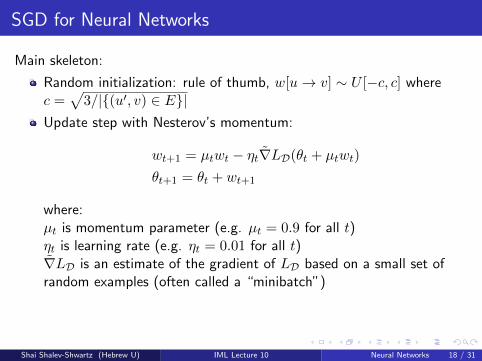
Main skeleton:
Random initialization: rule of thumb, w[u→ v] ∼ U [−c, c] wherec =
√3/|(u′, v) ∈ E|
Update step with Nesterov’s momentum:
wt+1 = µtwt − ηt∇LD(θt + µtwt)
θt+1 = θt + wt+1
where:µt is momentum parameter (e.g. µt = 0.9 for all t)ηt is learning rate (e.g. ηt = 0.01 for all t)∇LD is an estimate of the gradient of LD based on a small set ofrandom examples (often called a “minibatch”)
It is left to show how to calculate the gradient
Shai Shalev-Shwartz (Hebrew U) IML Lecture 10 Neural Networks 18 / 31
SGD for Neural Networks
Main skeleton:
Random initialization: rule of thumb, w[u→ v] ∼ U [−c, c] wherec =
√3/|(u′, v) ∈ E|
Update step with Nesterov’s momentum:
wt+1 = µtwt − ηt∇LD(θt + µtwt)
θt+1 = θt + wt+1
where:µt is momentum parameter (e.g. µt = 0.9 for all t)ηt is learning rate (e.g. ηt = 0.01 for all t)∇LD is an estimate of the gradient of LD based on a small set ofrandom examples (often called a “minibatch”)
It is left to show how to calculate the gradient
Shai Shalev-Shwartz (Hebrew U) IML Lecture 10 Neural Networks 18 / 31
Back-Propagation
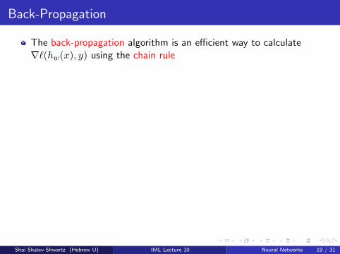
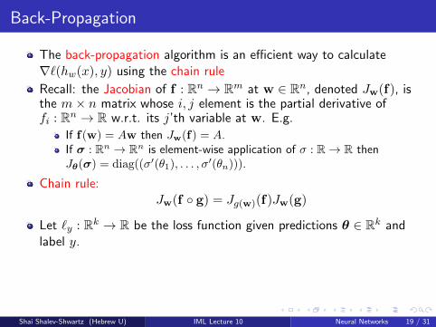
The back-propagation algorithm is an efficient way to calculate∇`(hw(x), y) using the chain rule
Recall: the Jacobian of f : Rn → Rm at w ∈ Rn, denoted Jw(f), isthe m× n matrix whose i, j element is the partial derivative offi : Rn → R w.r.t. its j’th variable at w. E.g.
If f(w) = Aw then Jw(f) = A.If σ : Rn → Rn is element-wise application of σ : R→ R thenJθ(σ) = diag((σ′(θ1), . . . , σ′(θn))).
Chain rule:Jw(f g) = Jg(w)(f)Jw(g)
Let `y : Rk → R be the loss function given predictions θ ∈ Rk andlabel y.
Shai Shalev-Shwartz (Hebrew U) IML Lecture 10 Neural Networks 19 / 31

Back-Propagation
The back-propagation algorithm is an efficient way to calculate∇`(hw(x), y) using the chain rule
Recall: the Jacobian of f : Rn → Rm at w ∈ Rn, denoted Jw(f), isthe m× n matrix whose i, j element is the partial derivative offi : Rn → R w.r.t. its j’th variable at w. E.g.
If f(w) = Aw then Jw(f) = A.
If σ : Rn → Rn is element-wise application of σ : R→ R thenJθ(σ) = diag((σ′(θ1), . . . , σ′(θn))).
Chain rule:Jw(f g) = Jg(w)(f)Jw(g)
Let `y : Rk → R be the loss function given predictions θ ∈ Rk andlabel y.
Shai Shalev-Shwartz (Hebrew U) IML Lecture 10 Neural Networks 19 / 31

Back-Propagation
The back-propagation algorithm is an efficient way to calculate∇`(hw(x), y) using the chain rule
Recall: the Jacobian of f : Rn → Rm at w ∈ Rn, denoted Jw(f), isthe m× n matrix whose i, j element is the partial derivative offi : Rn → R w.r.t. its j’th variable at w. E.g.
If f(w) = Aw then Jw(f) = A.If σ : Rn → Rn is element-wise application of σ : R→ R thenJθ(σ) = diag((σ′(θ1), . . . , σ′(θn))).
Chain rule:Jw(f g) = Jg(w)(f)Jw(g)
Let `y : Rk → R be the loss function given predictions θ ∈ Rk andlabel y.
Shai Shalev-Shwartz (Hebrew U) IML Lecture 10 Neural Networks 19 / 31

Back-Propagation
The back-propagation algorithm is an efficient way to calculate∇`(hw(x), y) using the chain rule
Recall: the Jacobian of f : Rn → Rm at w ∈ Rn, denoted Jw(f), isthe m× n matrix whose i, j element is the partial derivative offi : Rn → R w.r.t. its j’th variable at w. E.g.
If f(w) = Aw then Jw(f) = A.If σ : Rn → Rn is element-wise application of σ : R→ R thenJθ(σ) = diag((σ′(θ1), . . . , σ′(θn))).
Chain rule:Jw(f g) = Jg(w)(f)Jw(g)
Let `y : Rk → R be the loss function given predictions θ ∈ Rk andlabel y.
Shai Shalev-Shwartz (Hebrew U) IML Lecture 10 Neural Networks 19 / 31
Back-Propagation
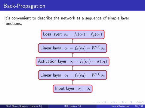
It’s convenient to describe the network as a sequence of simple layerfunctions:
Input layer: o0 = x
Linear layer: o1 = f1(o0) = W (1)o0
Activation layer: o2 = f2(o1) = σ(o1)
Linear layer: o3 = f3(o2) = W (3)o2
Loss layer: o4 = f4(o3) = `y(o3)
Shai Shalev-Shwartz (Hebrew U) IML Lecture 10 Neural Networks 20 / 31

Back-Propagation
Can write `(hw, (x, y)) = (fT+1 . . . f3 f2 f1)(x)
Denote Ft = fT+1 . . . ft+1 and δt = Jot(Ft), then
δt = Jot(Ft) = Jot(Ft−1 ft+1)
= Jft+1(ot)(Ft−1)Jot(ft+1) = Jot+1(Ft−1)Jot(ft+1)
= δt+1Jot(ft+1)
Note that
Jot(ft+1) =
W (t+1) for linear layer
diag(σ′(ot)) for activation layer
Using the chain rule again we obtain
JW (t)(`(hw, (x, y))) = δto>t−1
Shai Shalev-Shwartz (Hebrew U) IML Lecture 10 Neural Networks 21 / 31

Back-Propagation: Pseudo-code
Forward:
set o0 = x and for t = 1, 2, . . . , T set
ot = ft(ot−1) =
W (t)ot−1 for linear layer
σ(ot−1) for activation layer
Backward:
set δT+1 = ∇`y(oT ) and for t = T, T − 1, . . . , 1 set
δt = δt+1Jot(ft+1) = δt+1 ·
W (t+1) for linear layer
diag(σ′(ot)) for activation layer
For linear layers, set the gradient w.r.t. the weights in W (t) to be theelements of the matrix δto
>t−1
Shai Shalev-Shwartz (Hebrew U) IML Lecture 10 Neural Networks 22 / 31

Outline
1 Neural networks
2 Sample Complexity
3 Expressiveness of neural networks
4 How to train neural networks ?Computational hardnessSGDBack-Propagation
5 Convolutional Neural Networks (CNN)
6 Feature Learning
Shai Shalev-Shwartz (Hebrew U) IML Lecture 10 Neural Networks 23 / 31

Convolutional Networks
Designed for computer vision problems
Three main ideas:
Convolutional layers: use the same weights on all patches of the imagePooling layers: decrease image resolution (good for translationinvariance, for higher level features, and for runtime)Contrast normalization layers: let neurons “compete” with adjacentneurons
Shai Shalev-Shwartz (Hebrew U) IML Lecture 10 Neural Networks 24 / 31
Convolutional and Pooling
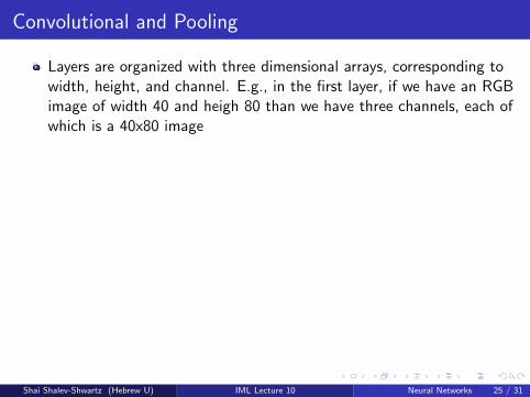
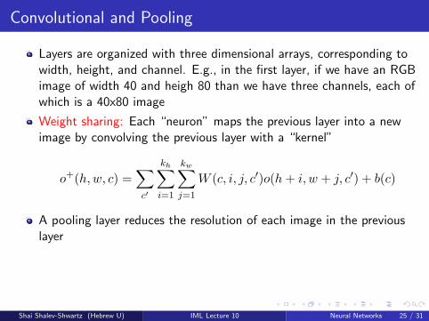
Layers are organized with three dimensional arrays, corresponding towidth, height, and channel. E.g., in the first layer, if we have an RGBimage of width 40 and heigh 80 than we have three channels, each ofwhich is a 40x80 image
Weight sharing: Each “neuron” maps the previous layer into a newimage by convolving the previous layer with a “kernel”
o+(h,w, c) =∑c′
kh∑i=1
kw∑j=1
W (c, i, j, c′)o(h+ i, w + j, c′) + b(c)
A pooling layer reduces the resolution of each image in the previouslayer
Shai Shalev-Shwartz (Hebrew U) IML Lecture 10 Neural Networks 25 / 31

Convolutional and Pooling
Layers are organized with three dimensional arrays, corresponding towidth, height, and channel. E.g., in the first layer, if we have an RGBimage of width 40 and heigh 80 than we have three channels, each ofwhich is a 40x80 image
Weight sharing: Each “neuron” maps the previous layer into a newimage by convolving the previous layer with a “kernel”
o+(h,w, c) =∑c′
kh∑i=1
kw∑j=1
W (c, i, j, c′)o(h+ i, w + j, c′) + b(c)
A pooling layer reduces the resolution of each image in the previouslayer
Shai Shalev-Shwartz (Hebrew U) IML Lecture 10 Neural Networks 25 / 31

Y LeCunMA Ranzato
Convolutional Network (ConvNet)
Non-Linearity: half-wave rectification, shrinkage function, sigmoidPooling: average, L1, L2, maxTraining: Supervised (1988-2006), Unsupervised+Supervised (2006-now)
input
83x83
Layer 1
64x75x75 Layer 2
64@14x14
Layer 3
256@6x6 Layer 4
256@1x1Output
101
9x9
convolution
(64 kernels)
9x9
convolution
(4096 kernels)
10x10 pooling,
5x5 subsampling6x6 pooling
4x4 subsamp
Shai Shalev-Shwartz (Hebrew U) IML Lecture 10 Neural Networks 26 / 31

Neural Networks as Feature Learning
“Feature Engineering” approach: expert constructs feature mappingφ : X → Rd. Then, apply machine learning to find a linear predictoron φ(x).
“Deep learning” approach: neurons in hidden layers can be thought ofas features that are being learned automatically from the data
Shallow neurons corresponds to low level features while deep neuronscorrespond to high level features
Shai Shalev-Shwartz (Hebrew U) IML Lecture 10 Neural Networks 27 / 31

Neural Networks as Feature LearningMulti-Layer Feature Learning
Taken from Yan LeCun’s deep learning tutorial
Shai Shalev-Shwartz (Hebrew U) IML Lecture 10 Neural Networks 28 / 31

Multiclass/Multitask/Feature Sharing/Representationlearning
Neurons in intermediate layers are shared by different tasks/classes
Only last layer is specific to task/class
Sometimes, network is optimized for certain classes, but theintermediate neurons are used as features for a new problem. This iscalled transfer learning. The last hidden layer can be thought of as arepresentation of the instance.
Shai Shalev-Shwartz (Hebrew U) IML Lecture 10 Neural Networks 29 / 31

Neural Networks: Current Trends
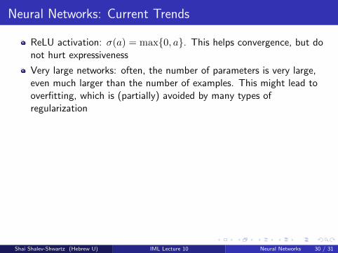
ReLU activation: σ(a) = max0, a. This helps convergence, but donot hurt expressiveness
Very large networks: often, the number of parameters is very large,even much larger than the number of examples. This might lead tooverfitting, which is (partially) avoided by many types ofregularization
Regularization: besides norm regularization, early stopping of SGDalso serves as a regularizer
Dropout: this is another form of regularization, in which someneurons are “muted” at random during training
Weight sharing (convolutional networks)
SGD tricks: momentum, Nesterov’s acceleration, other forms ofsecond order approximation
Training on GPU
Shai Shalev-Shwartz (Hebrew U) IML Lecture 10 Neural Networks 30 / 31
Neural Networks: Current Trends
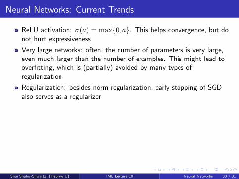
ReLU activation: σ(a) = max0, a. This helps convergence, but donot hurt expressiveness
Very large networks: often, the number of parameters is very large,even much larger than the number of examples. This might lead tooverfitting, which is (partially) avoided by many types ofregularization
Regularization: besides norm regularization, early stopping of SGDalso serves as a regularizer
Dropout: this is another form of regularization, in which someneurons are “muted” at random during training
Weight sharing (convolutional networks)
SGD tricks: momentum, Nesterov’s acceleration, other forms ofsecond order approximation
Training on GPU
Shai Shalev-Shwartz (Hebrew U) IML Lecture 10 Neural Networks 30 / 31

Neural Networks: Current Trends
ReLU activation: σ(a) = max0, a. This helps convergence, but donot hurt expressiveness
Very large networks: often, the number of parameters is very large,even much larger than the number of examples. This might lead tooverfitting, which is (partially) avoided by many types ofregularization
Regularization: besides norm regularization, early stopping of SGDalso serves as a regularizer
Dropout: this is another form of regularization, in which someneurons are “muted” at random during training
Weight sharing (convolutional networks)
SGD tricks: momentum, Nesterov’s acceleration, other forms ofsecond order approximation
Training on GPU
Shai Shalev-Shwartz (Hebrew U) IML Lecture 10 Neural Networks 30 / 31

Historical Remarks
1940s-70s:Inspired by learning/modeling the brain (Pitts, Hebb, and others)Perceptron Rule (Rosenblatt), Multilayer perceptron (Minksy andPapert)Backpropagation (Werbos 1975)
1980s – early 1990s:Practical Back-prop (Rumelhart, Hinton et al 1986) and SGD (Bottou)Initial empirical success
1990s-2000s:Lost favor to implicit linear methods: SVM, Boosting
2006 –:Regain popularity because of unsupervised pre-training (Hinton,Bengio, LeCun, Ng, and others)Computational advances and several new tricks allow training HUGEnetworks. Empirical success leads to renewed interest2012: Krizhevsky, Sustkever, Hinton: significant improvement ofstate-of-the-art on imagenet dataset (object recognition of 1000classes), without unsupervised pre-training
Shai Shalev-Shwartz (Hebrew U) IML Lecture 10 Neural Networks 31 / 31

Summary
Neural networks can be used to construct the ultimate hypothesisclass
Computationally, it’s impossible to train neural networks
. . . but, empirically, it works reasonably well
Leads to state-of-the-art on many real world problems
Biggest theoretical question: When does it work and why ?
Shai Shalev-Shwartz (Hebrew U) IML Lecture 10 Neural Networks 32 / 31


![Online Learning in Dynamic Environment · Introduction Dynamic Environment Conclusion Online Learning Regret Online Learning Online Learning [Shalev-Shwartz, 2011] Online learning](https://img.pdfslide.net/doc/110x75/5ec7294263e6ab666c4c6fc7/online-learning-in-dynamic-environment-introduction-dynamic-environment-conclusion.jpg)