Lecture 2 :: Decision Trees Learning

1 / 62

Designing a learning system

What to learn?Learning setting.Learning mechanism.Evaluation.

2 / 62

Prediction task

Figure 1: Prediction task :: Supervised learning

3 / 62

Lecture outline

MotivationDecision trees in generalClassification and regression trees (CART & ID3)

Building treeBinary questions, i.e. binary splitsBest split selection

Learning mechanism :: ID3 algorithmOver-fitting, pruningMore than one decision tree

4 / 62

Motivation :: Medical diagnosis example

Real world objects heart attack patients admitted to the hospital.Features age and medical symptoms indicating the patient’sconditions (got by measurements), like blood pressure.Output values high risk patients (G) and not high risk patients (F).Goal Identification of G- and F- patients on the basis ofmeasurements.

5 / 62

Motivation :: Medical diagnosis example (2)

Like a doctor, based on your experience, try to formulate criteria toidentify the patients:

1 1st question: Is the minimum systolic blood pressure over the initial24 hour period greater than 91?

2 If "no", then the patient is not high risk patient.3 If "yes", 2nd question: Is age greater than 62.5?4 If "no", then the patient is not high risk patient.5 If "yes", 3rd question: ...

6 / 62

Motivation :: Medical diagnosis example (3)

Figure 2: Medical diagnosis problem: classification rules (Credits: Leo Breimanet al., 1984)

7 / 62

Motivation :: Medical diagnosis example (4)

Like a machine learning expert, design a classifier based on the trainingdata ...

8 / 62

Decision trees in general

A tree is a graph G = (V ,E ) in which any two vertices are connected byexactly one simple path.

Figure 3: A tree in graph theory: any two vertices are connected by exactly onesimple path.

9 / 62

Decision trees in general (2)

A tree is called a rooted tree if one vertex has been designated the root,in which case the edges have a natural orientation, towards or away fromthe root.

Figure 4: A rooted tree

10 / 62

Decision trees in general (3)

A decision tree GDT = (VDT ,EDT ) is a rooted tree where VDT iscomposed of internal decision nodes and terminal leaf nodes.

Figure 5: A decision tree

11 / 62

Decision trees in general (4)

Decision tree learner building corresponds to building decision treeGDDT = (VD

DT ,EDDT ) based on a data set D = {〈x, y〉 : x ∈ X , y ∈ Y }. A

decision node t ∈ VDDT is a subset of D and the root node t = D. Each

leaf node is designated by an output value.

Decision tree learner building GDDT = (VD

DT ,EDDT ) corresponds to

repeated splits of subsets of D into descendant subsets, beginning with Ditself. Splits (decisions) are generated by questions.

12 / 62

Figure 6: A decision tree learner

13 / 62

Decision trees in general :: Geometrical point ofview

Tree-based methods partition the feature space into a set of regions, andthen fit a simple model in each region, for ex. majority vote forclassification, constant value for regression.

14 / 62

Classification trees :: Geometrical point of view (2)

Figure 7: Decision trees: a geometrical point of view (Credits: Alpaydin, 2004)

15 / 62

Regression trees :: Geometrical point of view

Figure 8: Regression trees: a geometrical point of view

16 / 62

Historical excursion

Classification trees: Y is a categorical output feature.Regression trees: Y is a numerical output feature.CART: ClAssification and Regression treesID3 → C4.5: classification trees

17 / 62

Historical excursion (2)

Figure 9: Two decision tree conceptions

11Automatic Interaction Detection(AID)

18 / 62

Once the decision tree learner is built,

an unseen instance is classified by starting at the root node and movingdown the tree branch corresponding to the feature values asked inquestions.

19 / 62

Milestone #1

To learn a decision tree, one has to

1 define question types,2 generate (best) splits,3 design/apply a learning mechanism,4 face troubles with over-fitting.

20 / 62

Notation

FeaturesAttr = {A1,A2, ...,AM},Values(Ai) is a set of all possible values for feature Ai .

Instances (i.e. feature vectors) x = 〈x1, x2, ..., xM〉,Output Values Y .DAiv = {〈x, y〉 ∈ D|xi = v}.

21 / 62

CART :: Question type definition

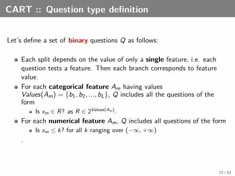
Let’s define a set of binary questions Q as follows:

Each split depends on the value of only a single feature, i.e. eachquestion tests a feature. Then each branch corresponds to featurevalue.For each categorical feature Am having valuesValues(Am) = {b1, b2, ..., bL}, Q includes all the questions of theform

Is xm ∈ R? as R ∈ 2Values(Am).

For each numerical feature Am, Q includes all questions of the formIs xm ≤ k? for all k ranging over (−∞,+∞)

.

22 / 62

CART :: Question type definition (2)

I.e. we restrict attention to recursive binary partitions, i.e. the featurespeace is partitioned into a set of rectangles.

23 / 62

ID3 :: Question type definition

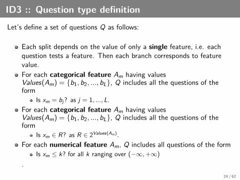
Let’s define a set of questions Q as follows:

Each split depends on the value of only a single feature, i.e. eachquestion tests a feature. Then each branch corresponds to featurevalue.For each categorical feature Am having valuesValues(Am) = {b1, b2, ..., bL}, Q includes all the questions of theform

Is xm = bj? as j = 1, ..., L.For each categorical feature Am having valuesValues(Am) = {b1, b2, ..., bL}, Q includes all the questions of theform

Is xm ∈ R? as R ∈ 2Values(Am).

For each numerical feature Am, Q includes all questions of the formIs xm ≤ k? for all k ranging over (−∞,+∞)

.24 / 62

ID3 :: Question type definition (2)

Figure 10: ID3: Non-binary splits

25 / 62

Milestone #2

To learn a decision tree, one has to

1 define question types,2 generate (best) splits,3 design/apply a learning mechanism,4 face troubles with over-fitting.

26 / 62

Best split generation :: Classification trees

We say a data set is pure (or homogenous) if it contains only a singleclass. If a data set contains several classes, then we say that the data setis impure (or heterogenous).

Decision tree classifier attempts to divide the M-dimensional feature spaceinto homogenous regions. The goal of adding new nodes to a tree is tosplit up the instance space so as to minimize the “impurity” of the trainingset.

⊕: 5, : 5 ⊕: 9, : 1heterogenous homogenous

high level of impurity low degree of impurity

27 / 62

Best split generation :: Classification trees (2)

1. Define the node proportions p(j |t), j = 1, ..., c, to be the proportionof the instances x, 〈x, j〉 ∈ t, so that

∑cj=1 p(j |t) = 1.

2. Define a measure i(t) of the impurity of t as a nonnegativefunction Φ of the p(1|t), p(2|t), ..., p(c|t),

i(t) = Φ(p(1|t), p(2|t), ..., p(c|t)), (1)

such thatΦ( 1

c ,1c , ...,

1c ) = max , i.e. the node impurity is largest when all

examples are equally mixed together in it.Φ(1, 0, ..., 0) = 0,Φ(0, 1, ..., 0) = 0, ...,Φ(0, 0, ..., 1) = 0, i.e. the nodeimpurity is smallest when the node contains instances of only one class

3. Define the goodness of split s to be the decrease in impurity∆i(s, t) = i(t)− pL ∗ i(tL)− pR ∗ i(tR). pL is a proportin of examplesin t going to tL, similarly with pR .

28 / 62

Best split generation :: Classification trees (3)

Figure 11: Split in decision tree (Credits: Leo Breiman et al., 1984)

4. Define a candidate set S of splits at each node: the set Q ofquestions generates a set S of splits of every node t. Find split s∗with the largest decrease in impurity: ∆i(s∗, t) = maxs∈S∆i(s, t).

29 / 62

Best split generation :: Classification trees (4)

5. Discuss four splitting criteria:Misclassification Error i(t)MisclassificationError ,Information Gain i(t)InformationGain,Gini Index i(t)GiniIndex .

30 / 62

Best split generation :: Classification trees (5)

i(t)MisclassificationError = 1−maxj=1,...,cp(j |t) (2)

⊕: 0, : 6 ⊕: 1, : 5 ⊕: 2, : 4 ⊕: 3, : 3

M. E. 1− 66 = 0 1− 5

6 = 0, 17 1− 46 = 0, 33 1− 3

6 = 0, 5

31 / 62

Best split generation :: Classification trees (6)

i(t)InformationGain = −c∑

j=1p(j |t) ∗ log(p(j |t). (3)

∆i(sAk , t)InformationGain = i(t)−∑

v∈Values(Ak )

ptv ∗ i(tv ) = H(t)−∑

v∈Values(Ak )

|tv ||t| H(tv ) (4)

where tv is the subset of t for which attribute Ak has value v .

Gain(s, t) = ∆i(s, t)InformationGain (5)

32 / 62

Best split generation :: Classification trees (7)

The information gain favors features with many values over those withfew values (many values, many branches, impurity can be much less).

ExampleLet’s consider the feature Date. It has so many values that it is bound toseparate the training examples into very small subsets. As it has a highinformation gain relative to the training data, it is probably selected for theroot node. But prediction behind the training examples is poor. Let’sincorporate an alternative measure Gain ratio that takes into account thenumber of values of a feature.

33 / 62

Best split generation :: Classification trees (8)

GainRatio(sAk , t) =Gain(sAk , t)

SplitInformation(sAk , t), (6)

where

SplitInformation(sAk , t) = −∑

v∈Values(Ak)

|tv ||t| log2

|tv ||t| , (7)

SplitInformation(sAk , t) is the entropy of t with respect to the split sAk ,i.e. to the values of feature Ak .

34 / 62

Best split generation :: Classification trees (9)

i(t)GiniIndex = 1−∑jp2(j |t). (8)

35 / 62

Best split generation :: Classification trees (10)

⊕: 0 ⊕: 1 ⊕: 2 ⊕: 3: 6 : 5 ⊕: 4 ⊕: 3

Gini 0 0.278 0.444 0.5Entropy 0 0.65 0.92 1.0M.E. 0 0.17 0.333 0.5

For two classes (c = 2), if p is the proportion in the class "1", themeasures are:

Misclassification error: 1−max(p, 1− p)

Entropy: −p ∗ logp − (1− p) ∗ log(1− p)

Gini: 2p ∗ (1− p)

36 / 62

Best split generation :: Classification trees (11)

Figure 12: Selection the best split :: Misclassification vs. Entropy vs. Gini

See http://ufal.mff.cuni.cz/~hladka/lab/entropy-gini-miss.R.

37 / 62

Milestone #3

To learn a decision tree, one has to

1 define question types,2 generate (best) splits: classification trees, regression trees,3 design/apply a learning mechanism,4 face troubles with over-fitting.

38 / 62

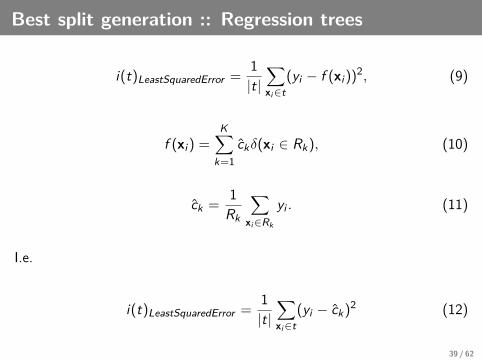
Best split generation :: Regression trees

i(t)LeastSquaredError =1|t|

∑xi∈t

(yi − f (xi))2, (9)

f (xi) =K∑

k=1ckδ(xi ∈ Rk), (10)

ck =1Rk

∑xi∈Rk

yi . (11)

I.e.

i(t)LeastSquaredError =1|t|

∑xi∈t

(yi − ck)2 (12)

39 / 62

ck as an average of yi for all training instances xi falling into t (i.e. intoRk) minimizes i(t)LeastSquaredError .

The proof is based on seeing that the number which minimizes∑i(yi − a)2 is a = 1

N∑

i yi .

40 / 62

Best split generation :: Regression trees (2)

2. Define the goodness of split s to be

∆i(s, t) = i(t)− i(tL)− i(tR) (13)

.3. Define a candidate set S of splits at each node: the set Q of

questions generates a set S of splits of every node t. Find split s∗ :∆i(s∗, t) = mins∈S∆i(s, t).

41 / 62

Milestone #4

To learn a decision tree, one has to

1 define question types,2 generate (best) splits: classification trees, regressiontrees,

3 design/apply a learning mechanism,4 face troubles with over-fitting.

42 / 62

Learning mechanism :: ID3 algorithm(D, Y , Attr)

Create a Root node for the tree.If ∀x, 〈x, y〉 ∈ D : y = 1, return single node tree Root with label =’+’.If ∀x, 〈x, y〉 ∈ D : y = −1, return single node tree Root with label =’-’.If Attr = ∅, return a single node tree Root with label = mostcommon value of Y in D, i.e. n = maxv

∑v∈Y ,〈x,y〉∈D δ(v ,Y (x)).

OtherwiseA := Splitting Criterion(Attr)Root := A∀v ∈ Values(A)

Add a new tree branch below Root, corresponding to the test A(x) = vIf Dv = ∅ then below this new branch add a leaf node with label =n = maxv

∑v∈Values(Y ),〈x,y〉∈D δ(v ,Y (x)); else below this new branch

add the subtree ID3(Dv ,Y ,Attr − {A})

Return(Root).43 / 62

Learning mechanism :: ID3 algorithm :: Comments

ID3 is a recursive partitioning algorithm (divide & conquer), performstop-down tree construction.ID3 performs a simple-to-complex, hill-climbing search through Hguided by a particular splitting criterion.ID3 maintains only a single current hypothesis. So ID3 for example isnot able to determine any other decision trees consistent with trainingdata.ID3 does not employ backtracking.

44 / 62

Milestone #5

To learn a decision tree, one has to

1 define question types,2 generate (best) splits: classification trees, regressiontrees,

3 design/apply a learning mechanism,4 face troubles with over-fitting.

45 / 62

Over-Fitting

The divide and conquer algorithm partitions the data until every leafcontains examples of a single value, or until further partitioning isimpossible because two examples have the same values for each featurebut belong to different classes. Consequently, if there are no noisyexamples, the decision tree will correctly classify all training examples.

Over-fitting can be avoided by a stopping criterion that prevents some setsof training examples from being subdivided, or by removing some of thestructure of the decision tree after it has been produced.

46 / 62

Over-Fitting

When a node t was reached such that no significant decrease inimpurity was possible (i.e. maxs∆i(s, t) < β), then t was not splitand became a terminal node. The class of this terminal node isdetermined as follows: majority vote for classification and averagevalue for regression. But ...

If β is set too low, then there is too much splitting and the tree is toolarge. This tree might overfit the data.Increasing β: there maybe nodes t such that maxs∆i(s, t) < β is small.But the descendants nodes tL and tR of t may have splits with largedecreases in impurity. By declaring t terminal, one looses the goodsplits on tL or tR . This tree might not capture the important structure.

Preferred strategy: Grow a large tree T0, stopping the splittingprocess when only some minimum node size (say 5) is reached. Thenprune T0 using some pruning criteria.

47 / 62

Pruning :: C4.5 :: Reduced error pruning

Figure 13: Reduced Error Pruning

subtrees T ∗i already pruned,let T ∗f be the subtree corresponding to the most frequent value of Ain the data,let L be a leaf labelled with the most frequent class in the data.

48 / 62

Pruning :: C4.5 :: Reduced error pruning (2)

Split the data into training D and validation Dv sets.Build a tree T to fit the data D.Evaluate impact of pruning each possible node on validation set Dv :

let ET be the sample error rate of T on Dv ,let ET∗

fbe the sample error rate of T ∗

f on Dv ,let EL be the sample error rate of L on Dv .

Let UCF (ET , |Dv ), UCF (ET∗f , |Dv ), UCF (EL, |Dv ) be the threecorresponding estimated error rates (via confidence intervals).

Depending on whichever is lower, C4.5

leaves T unchanged,replaces T by the leaf L, orreplaces T by its subtree T ∗f .

49 / 62

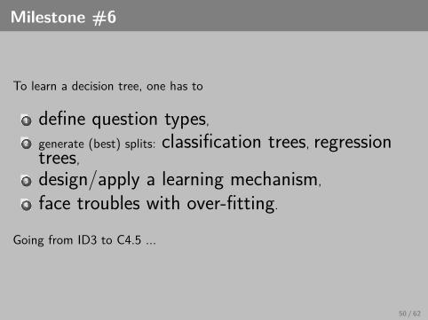
Milestone #6

To learn a decision tree, one has to

1 define question types,2 generate (best) splits: classification trees, regressiontrees,

3 design/apply a learning mechanism,4 face troubles with over-fitting.

Going from ID3 to C4.5 ...

50 / 62

ID3 :: Incorporating continuous-valued features

ID3 is originally designed with two restrictions:

1 Discrete-valued predicted feature.2 Discrete-valued features tested in the decision tree nodes. → Let’s

extend it for the continuous-valued features.

For a continuous-valued feature A, define a boolean-valued feature Ac sothat if A(x) ≤ c then Ac(x) = 1 else Ac(x) = 0.

51 / 62

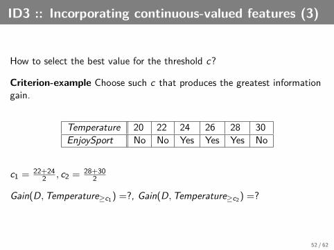
ID3 :: Incorporating continuous-valued features (3)

How to select the best value for the threshold c?

Criterion-example Choose such c that produces the greatest informationgain.

Temperature 20 22 24 26 28 30EnjoySport No No Yes Yes Yes No

c1 = 22+242 , c2 = 28+30

2

Gain(D,Temperature≥c1) =?, Gain(D,Temperature≥c2) =?

52 / 62

ID3 :: Handling training examples with missingfeature values

Consider the situation in which Gain(D,A) is to be calculated at node t inthe decision tree. Suppose that 〈x, c(x)〉 is one of the training examples inD and that the value A(x) is unknown.

Possible solutions

Assign the value that is most common among training examples atnode t.Alternatively, assign the most common value among examples at nodet that have the classification c(x).

53 / 62

Milestone #7

To learn a decision tree, one has to

1 define question types,2 generate (best) splits: classification trees, regressiontrees,

3 design/apply a learning mechanism,4 face troubles with over-fitting.

Going from ID3 to C4.5 ...Having a bag of decision trees ...

54 / 62

More than one decision tree

Some techniques, often called ensemble methods, construct more than onedecision tree, e.g.

Boosted Trees.

55 / 62

More than one decision tree :: Boosted trees

In general,

The more data, the better :: an approach of ’resampling’Same learning mechanism, different classifiers h1, h2, ..., hn.

Boosting is a procedure that combines the outputs of many weakclassifiers to produce a powerfull "committee". A weak classifier has anerror rate only slightly better than random guessing.

Schapire’s strategy: Change the distribution over the training examplesin each iteration, feed the resulting sample into the weak classifier, andthen combine the resulting hypotheses into a voting ensemble, which, inthe end, would have a boosted classification accuracy.

56 / 62

More than one decision tree :: Boosted trees (2)

AdaBoost.M1 algorithm

An iterative algorithm that selects ht given the performance obtainedby weak learners h1 → ht−1At each step t

modifies training data distribution in order to favour hard-to-classifyexamples according to previous weak classifiers,trains a new weak classifier ht ,selects the new weight αt of ht by optimizing a final classifier

stops when impossible to find a weak classifier being better thanchance,outputs a final classifier being the weighted sum of all weak classifiers.

57 / 62

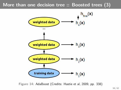
More than one decision tree :: Boosted trees (3)

Figure 14: AdaBoost (Credits: Hastie et al, 2009, pp. 338)58 / 62

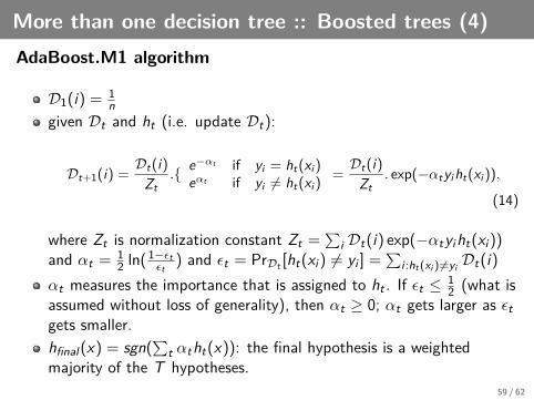
More than one decision tree :: Boosted trees (4)AdaBoost.M1 algorithm

D1(i) = 1n

given Dt and ht (i.e. update Dt):

Dt+1(i) =Dt(i)Zt

.{ e−αt if yi = ht(xi)eαt if yi 6= ht(xi)

=Dt(i)Zt

. exp(−αtyiht(xi)),

(14)

where Zt is normalization constant Zt =∑

i Dt(i) exp(−αtyiht(xi))and αt = 1

2 ln(1−εtεt

) and εt = PrDt [ht(xi) 6= yi ] =∑

i :ht(xi )6=yi Dt(i)αt measures the importance that is assigned to ht . If εt ≤ 1

2 (what isassumed without loss of generality), then αt ≥ 0; αt gets larger as εtgets smaller.hfinal(x) = sgn(

∑t αtht(x)): the final hypothesis is a weighted

majority of the T hypotheses.59 / 62

Final remarks

⊕ Decision tree based classifiers are readily interpretable by humans. Instability of trees: learned tree structure is sensitive to the trainingdata, so that a small change to the data can result in a very differentset of splits.

60 / 62

For more details refer to

Hastie, T. et al. The Elements of Statistical Learning. Springer, 2009,

Section 9.2; Chapter 10 pp. 337–341,

61 / 62

References

Breiman Leo, Friedman Jerome H., Olshen Richard A., Stone CharlesJ. Classification and Regression Trees. Chapman & Hall/CRC, 1984.Boosting: A sample example: http://www.cs.toronto.edu/~hinton/csc321/notes/boosting.pdf

Hunt, E. B. Concept Learning: An Information Processing Problem,Wiley. 1962.Morgan, J. N., Sonquist, J. A. Problems in the analysis of surveydata, and a proposal. Journal of the American Statistical Association58, pp. 415–434. 1963.Quinlan, J. R. Discovering rules from large collections of examples: Acase study, in D. Michie, ed., Expert Systems in the Micro ElectronicAge. Edinburgh University Press. 1979.Quinlan, J. R. C4.5: Programs for Machine Learning, MorganKaufmann, San Mateo, California. 1993.

62 / 62