Embed Size (px)
Citation preview
Introduction to Machine LearningCMSC 422
Ramani Duraiswami
Decision Trees Wrapup, Overfitting
Slides adapted from Profs. Carpuat and Roth

A decision tree to distinguish homes in
New York from homes in San
Francisco
http://www.r2d3.us/visual-intro-to-machine-learning-part-1/
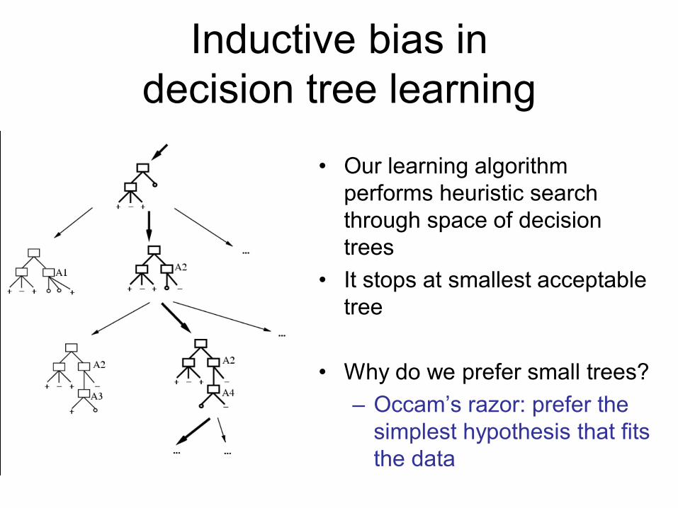
Inductive bias in
decision tree learning
• Our learning algorithm
performs heuristic search
through space of decision
trees
• It stops at smallest acceptable
tree
• Why do we prefer small trees?
– Occam’s razor: prefer the
simplest hypothesis that fits
the data
Evaluating the learned hypothesis ℎ
• Assume
– we’ve learned a tree ℎ using the top-down
induction algorithm
– It fits the training data perfectly
• Is it guaranteed to be a good hypothesis?
Training error is not sufficient
• We care about generalization to new
examples
• A tree can classify training data perfectly,
yet classify new examples incorrectly
– Because training examples are incomplete --
only a sample of data distribution
• a feature might correlate with class by coincidence
– Because training examples could be noisy
• e.g., accident in labeling
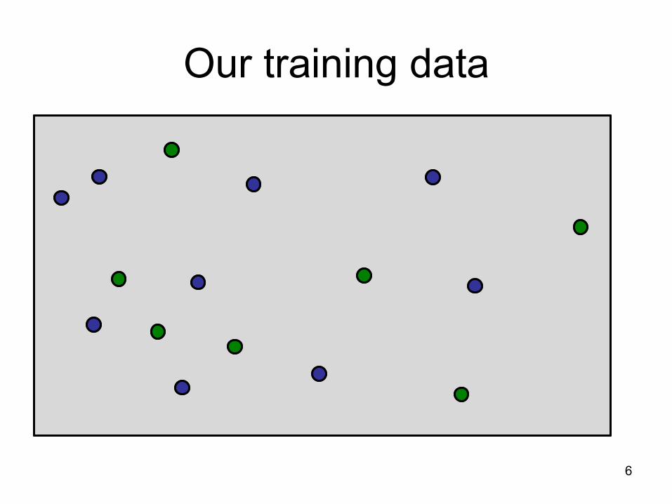
Our training data
6

The instance space
]]
]]]]
7
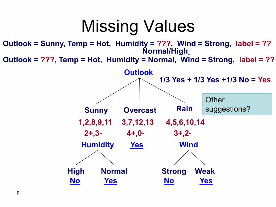
Missing Values
8
Outlook
Overcast Rain
3,7,12,13 4,5,6,10,14
3+,2-
Sunny
1,2,8,9,11
4+,0-2+,3-
YesHumidity Wind
NormalHigh
No
WeakStrong
No YesYes
Outlook = ???, Temp = Hot, Humidity = Normal, Wind = Strong, label = ??
1/3 Yes + 1/3 Yes +1/3 No = Yes
Outlook = Sunny, Temp = Hot, Humidity = ???, Wind = Strong, label = ?? Normal/High
Other
suggestions?
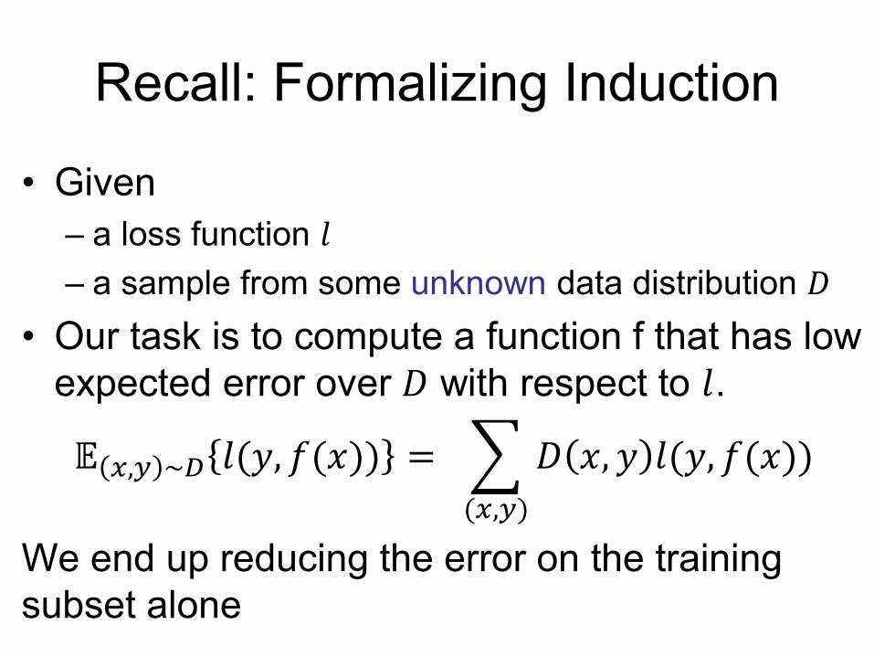
Recall: Formalizing Induction
• Given
– a loss function 𝑙
– a sample from some unknown data distribution 𝐷
• Our task is to compute a function f that has low
expected error over 𝐷 with respect to 𝑙.
𝔼 𝑥,𝑦 ~𝐷 𝑙(𝑦, 𝑓(𝑥)) =
(𝑥,𝑦)
𝐷 𝑥, 𝑦 𝑙(𝑦, 𝑓(𝑥))
We end up reducing the error on the training
subset alone
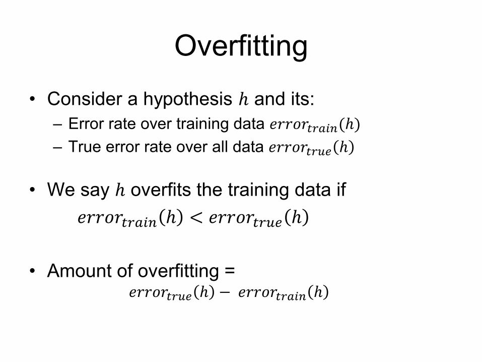
Overfitting
• Consider a hypothesis ℎ and its:
– Error rate over training data 𝑒𝑟𝑟𝑜𝑟𝑡𝑟𝑎𝑖𝑛(ℎ)
– True error rate over all data 𝑒𝑟𝑟𝑜𝑟𝑡𝑟𝑢𝑒 ℎ
• We say ℎ overfits the training data if
𝑒𝑟𝑟𝑜𝑟𝑡𝑟𝑎𝑖𝑛 ℎ < 𝑒𝑟𝑟𝑜𝑟𝑡𝑟𝑢𝑒 ℎ
• Amount of overfitting =𝑒𝑟𝑟𝑜𝑟𝑡𝑟𝑢𝑒 ℎ − 𝑒𝑟𝑟𝑜𝑟𝑡𝑟𝑎𝑖𝑛 ℎ
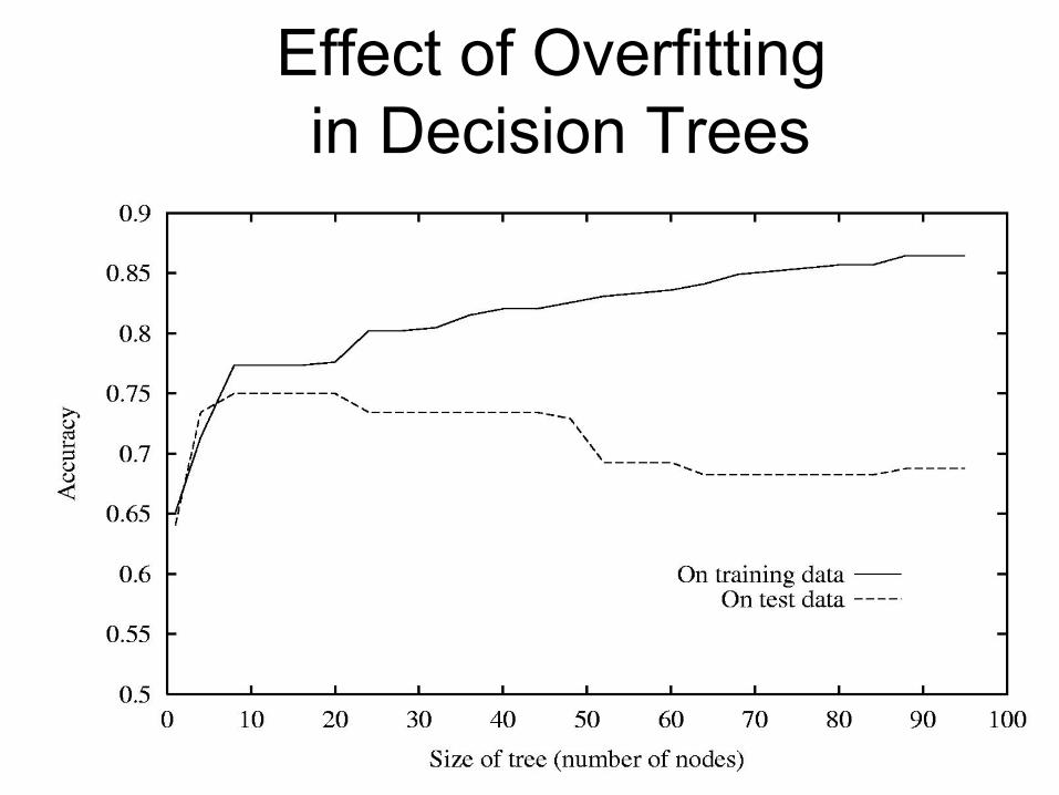
Effect of Overfitting
in Decision Trees
Evaluating on test data
• Problem: we don’t know 𝑒𝑟𝑟𝑜𝑟𝑡𝑟𝑢𝑒 ℎ !
• Solution:
– we set aside a test set
• some examples that will be used for evaluation
– we don’t look at them during training!
– after learning a decision tree, we calculate
𝑒𝑟𝑟𝑜𝑟𝑡𝑒𝑠𝑡 ℎ
Underfitting/Overfitting
• Underfitting
– Learning algorithm had the opportunity to learn more
from training data, but didn’t
– Or didn’t have sufficient data to learn from
• Overfitting
– Learning algorithm paid too much attention to
idiosyncrasies of the training data; the resulting tree
doesn’t generalize
• What we want:
– A decision tree that neither underfits nor overfits
– Because it is expected to do best in the future
Pruning a decision tree
• Prune = remove leaves and assign
majority label of the parent to all items
• Prune the children of S if:
– all children are leaves, and
– the accuracy on the validation set does not
decrease if we assign the most frequent class
label to all items at S.
14
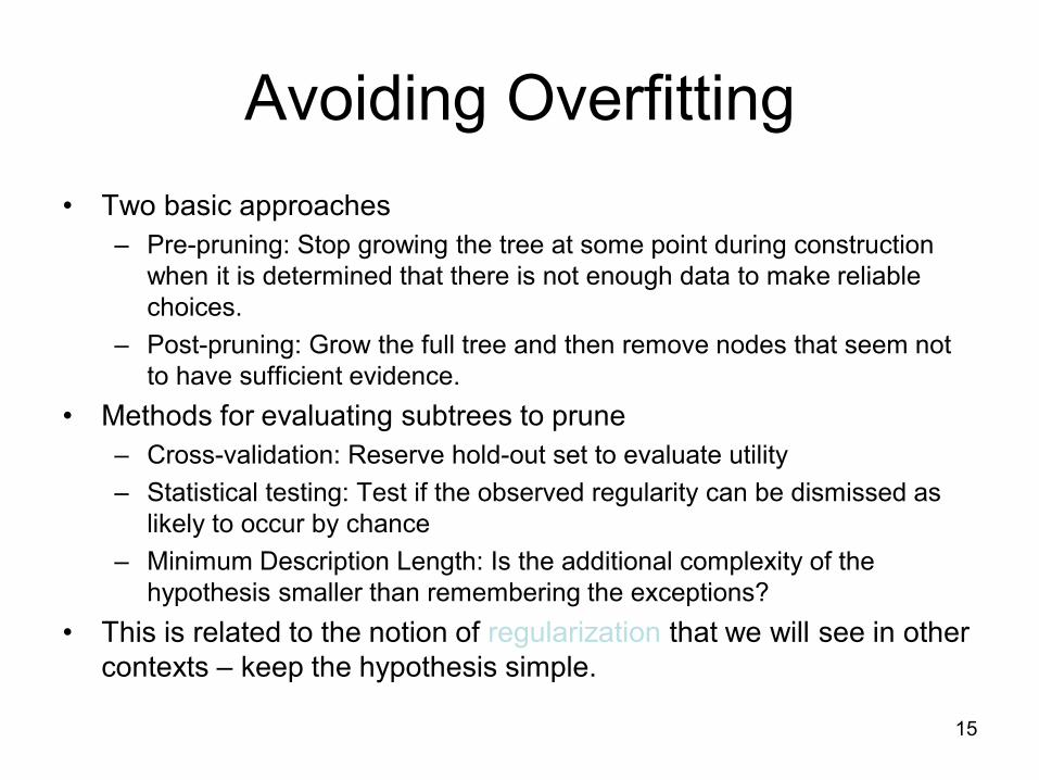
Avoiding Overfitting
• Two basic approaches
– Pre-pruning: Stop growing the tree at some point during construction
when it is determined that there is not enough data to make reliable
choices.
– Post-pruning: Grow the full tree and then remove nodes that seem not
to have sufficient evidence.
• Methods for evaluating subtrees to prune
– Cross-validation: Reserve hold-out set to evaluate utility
– Statistical testing: Test if the observed regularity can be dismissed as
likely to occur by chance
– Minimum Description Length: Is the additional complexity of the
hypothesis smaller than remembering the exceptions?
• This is related to the notion of regularization that we will see in other
contexts – keep the hypothesis simple.
15

Size of tree
Accuracy
On test data
On training data
Overfitting
• A decision tree overfits the training data when its accuracy on the training data goes up but its accuracy on unseen data goes down
16

Model complexity
Empirical
Error
Overfitting
17
• Empirical error (= on a given data set):
The percentage of items in this data set
are misclassified by the classifier f.
Model complexity
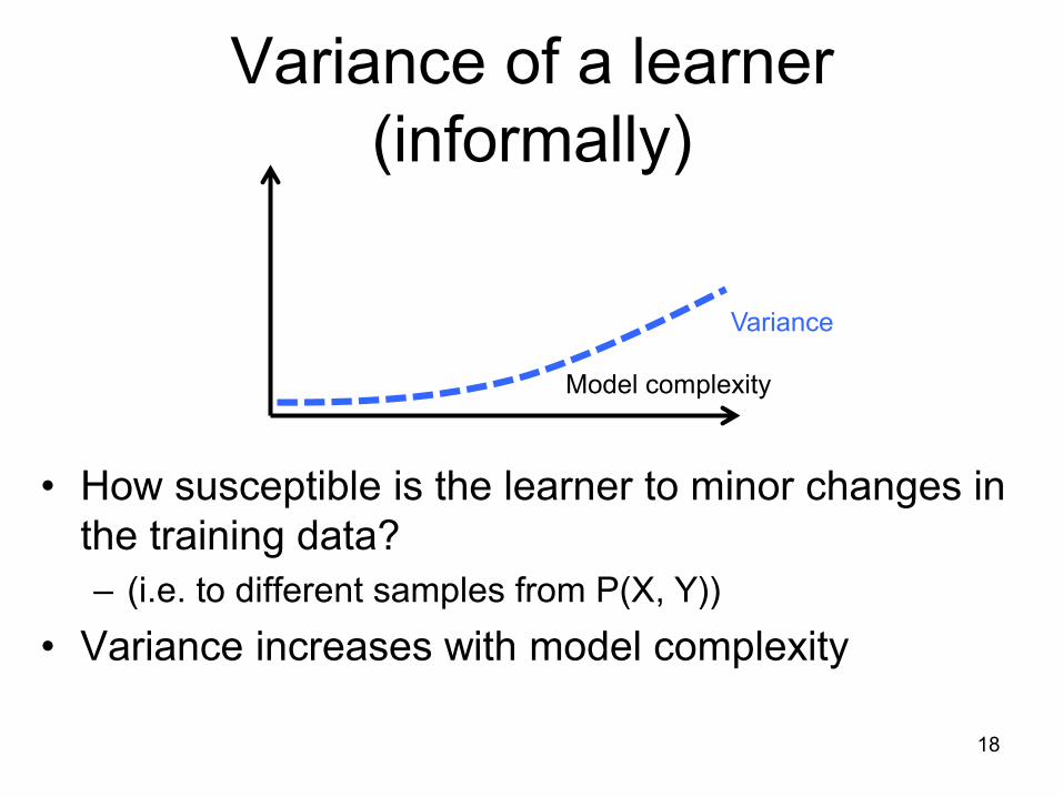
Variance of a learner
(informally)
• How susceptible is the learner to minor changes in
the training data?
– (i.e. to different samples from P(X, Y))
• Variance increases with model complexity
18
Variance
Model complexity
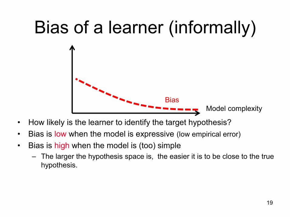
Bias of a learner (informally)
• How likely is the learner to identify the target hypothesis?
• Bias is low when the model is expressive (low empirical error)
• Bias is high when the model is (too) simple
– The larger the hypothesis space is, the easier it is to be close to the true
hypothesis.
19
Bias

Model complexity
Expected
Error
Impact of bias and variance
20
• Expected error ≈ bias + variance
Variance
Bias
Model complexity
Expected
Error
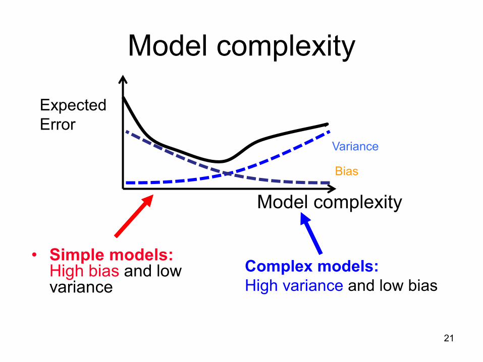
Model complexity
21
• Simple models: High bias and low variance
Variance
Bias
Complex models:
High variance and low bias

Underfitting Overfitting
Model complexity
Expected
Error
Underfitting and Overfitting
22
• Simple models: High bias and low variance
Variance
Bias
Complex models:
High variance and low bias
This can be made more accurate for some loss functions.
We will develop a more precise and general theory that
trades expressivity of models with empirical error

Expectation
• X is a discrete random variable with
distribution P(X):
• Expectation of X (E[X]), aka. the mean of X (μX)
E[X} = x P(X=x)X := μX
• Expectation of a function of X (E[f(X)])
E[f(X)} = x P(X=x)f(x)
• If X is continuous, replace sums with
integrals23
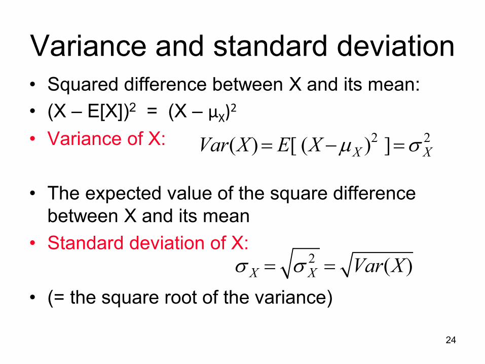
Variance and standard deviation• Squared difference between X and its mean:
• (X – E[X])2 = (X – μX)2
• Variance of X:
• The expected value of the square difference
between X and its mean
• Standard deviation of X:
• (= the square root of the variance)
24
Var(X)= E[ (X -mX )2 ]=s X
2
s X = s X2 = Var(X)
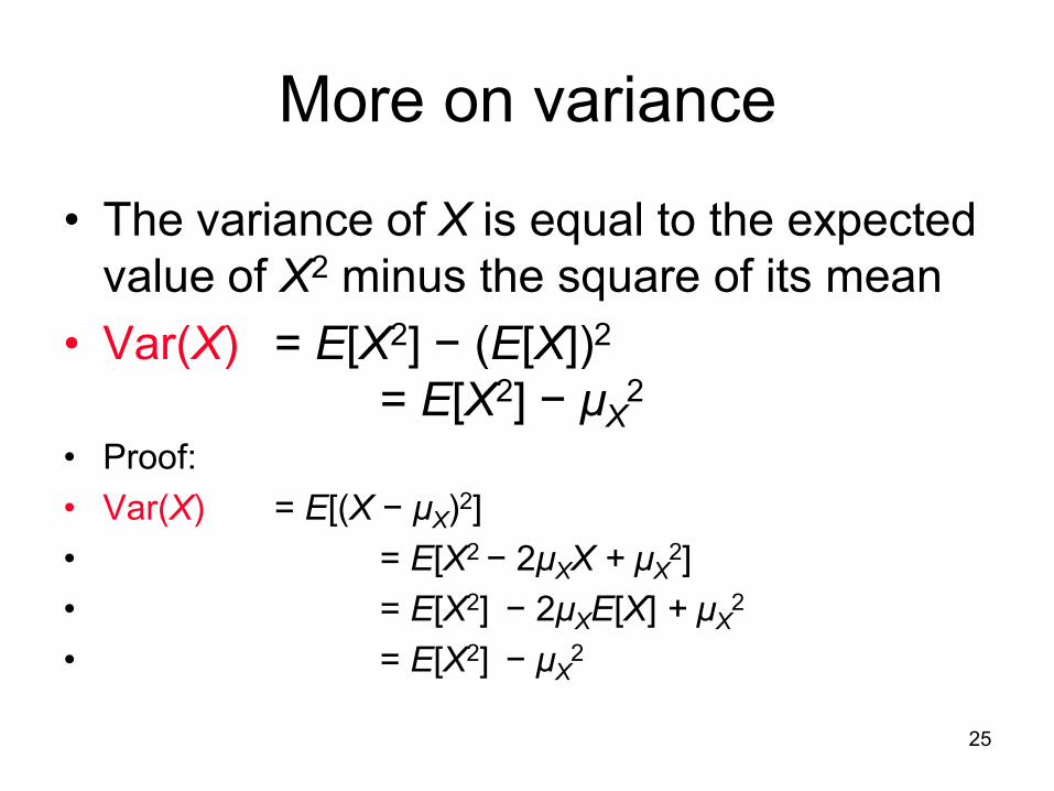
More on variance
• The variance of X is equal to the expected
value of X2 minus the square of its mean
• Var(X) = E[X2] − (E[X])2
= E[X2] − μX2
• Proof:
• Var(X) = E[(X − μX)2]
• = E[X2 − 2μXX + μX2]
• = E[X2] − 2μXE[X] + μX2
• = E[X2] − μX2
25
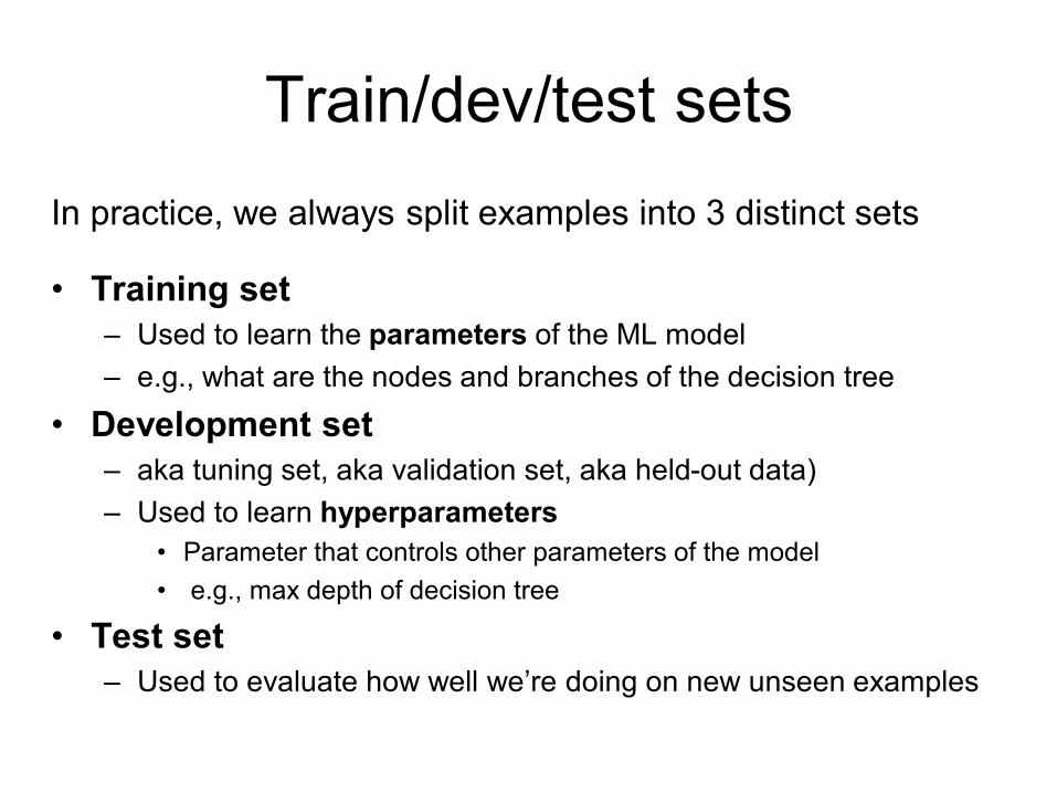
Train/dev/test sets
In practice, we always split examples into 3 distinct sets
• Training set
– Used to learn the parameters of the ML model
– e.g., what are the nodes and branches of the decision tree
• Development set
– aka tuning set, aka validation set, aka held-out data)
– Used to learn hyperparameters
• Parameter that controls other parameters of the model
• e.g., max depth of decision tree
• Test set
– Used to evaluate how well we’re doing on new unseen examples

Cardinal rule of machine learning:
Never ever touch
your test data!