Embed Size (px)
Citation preview
Chapter 1 1 Final.
PART I: PRELIMINARIESChapter 1: Introduction to Macroeconomics
J. Bradford DeLonghttp://www.j-bradford-delong.net/
9,118 words
Questions
1. How much richer are we than our parents were at our age?
2. How much richer will our children be than our grandparents were?
3. Will changing jobs be easy or hard in five years?
4. How many of us will have jobs in five years?
5. Will the businesses we work for vanish as demand for the products they make
dries up?
6. Will inflation make us poor by destroying our savings or rich by eliminating
our debts?
Chapter 1 2 Final.
1.1 Overview
What Is Macroeconomics?
What is macroeconomics? Macroeconomics is that subdiscipline of economics that tries
to answer the six questions that begin this chapter. Answers to all these questions depend
on what is happening to the economy as a whole, the economy-in-the-large, the
macroeconomy. "Macro" is, after all, nothing but a prefix for "large." Macroeconomics is
that branch of economics related to the economy as a whole.
Macroeconomists' principal task is to try to figure out why overall economic activity rises
and falls. Why are measures like the total value of all production, the total income of
workers and property owners, the total number of people employed, or the unemployment
rate higher in some years than in others? Macroeconomists also attempt to understand
what determines the level and rate of change of overall prices. The proportional rate of
change in the price level has a name you have undoubtedly heard thousands of times: it is
called the inflation rate. Finally, along the way macroeconomists study other variables--
like interest rates, stock market values, and exchange rates--that play a major role in
determining the overall levels of production, income, employment, and prices.
Why Macroeconomics Matters
Why does macroeconomics matter? Why should we care about the questions at the heart
of macroeconomics? There are at least three reasons.
Chapter 1 3 Final.
Cultural Literacy
First (but least important), macroeconomics is a matter of cultural literacy. Much
discussion in newspapers, on television, and at parties concerns the macroeconomy,
which should not be surprising: the twentieth-century U.S. economy has been, all in all,
extraordinarily successful. Today we are on average some 50% richer than our parents
were when they were our age. If economic growth continues at its recent pace, our
children may be five or more times as rich as our grandparents were.
In su, our modern industrial economy has delivered increases in material prosperity and
living standards that no previous generation ever saw. (We shall discuss this topic at
greater length in Chapter 5.) This increasing material prosperity means that the economy
has a cultural salience today it did not have in previous centuries, when productivity was
stagnant and material standards of living improved only as fast as a glacier moves.
Thus, if you want to follow and participate in public debates and discussions, you need to
know about macroeconomics. If you don't, you won't underwstand news reports on
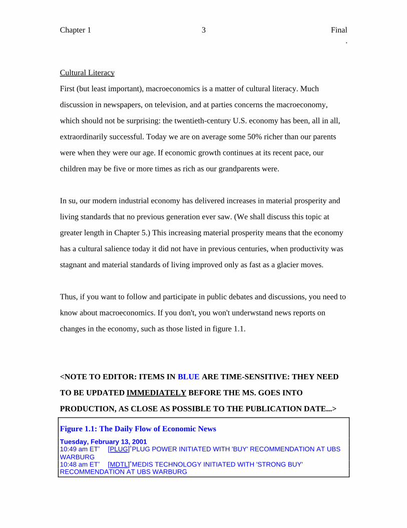
changes in the economy, such as those listed in figure 1.1.
<NOTE TO EDITOR: ITEMS IN BLUE ARE TIME-SENSITIVE: THEY NEED
TO BE UPDATED IMMEDIATELY BEFORE THE MS. GOES INTO
PRODUCTION, AS CLOSE AS POSSIBLE TO THE PUBLICATION DATE...>
Figure 1.1: The Daily Flow of Economic News
Tuesday, February 13, 200110:49 am ET [PLUG] PLUG POWER INITIATED WITH 'BUY' RECOMMENDATION AT UBSWARBURG10:48 am ET [MDTL] MEDIS TECHNOLOGY INITIATED WITH 'STRONG BUY'RECOMMENDATION AT UBS WARBURG
Chapter 1 4 Final.
10:48 am ET [APWR] ASTROPOWER INITIATED WITH 'BUY' RECOMMENDATION AT UBSWARBURG10:48 am ET [CPST] CAPSTONE INITIATED WITH 'BUY' RECOMMENDATION AT UBSWARBURG10:47 am ET [FCEL] FUEL CELL ENERGY INITIATED WITH 'STRONG BUY'RECOMMENDATION AT UBS WARBURG10:46 am ET [CF] CHARTER ONE FINANCIAL INITIATED WITH 'BUY' RECOMMENDATIONAT UBS WARBURG10:45 am ET [FTO] FRONTIER OIL Q4 EARNS 5 CENTS VS. 90 CENTS YR AGO QTR10:44 am ET [$BTK,ATIS] AMEX BIOTECH INDEX CLIMBS 1.7%, ADVANCED TISSUESCIENCES UP 4.3%10:33 am ET [$GIN,VRSN] GOLDMAN SACHS INTERNET INDEX RISES 3.1%, LED BYVERISIGN UP 7.9%10:22 am ET [$SOX,RMBS] PHILADELPHIA SEMICONDUCTOR INDEX CLIMBS 3.5%, LEDBY RAMBUS UP 7.3%10:15 am ET [NVLS] NOVELLUS SYSTEMS CUT TO 'SELL' FROM 'HOLD' AT WELLSFARGO VAN KASPER10:14 am ET [OPMR] OPTIMAL ROBOTICS DROPPED TO 'MARKET OUTPERFORM'FROM 'STRONG BUY' AT ROBERT W. BAIRD10:12 am ET [NFB,CBNY] NORTH FORK TO ACQUIRE COMMERCIAL BANK OF NEWYORK FOR $175 MLN IN CASH10:11 am ET O'NEILL, IN HOUSE TESTIMONY, CALLS ON CONGRESS TO QUICKLYENACT TAX RELIEF PACKAGE10:10 am ET TREASURY'S O'NEILL: BUSH TAX PACKAGE 'JUST RIGHT' IN SIZE10:04 am ET [$COMPQ] NASDAQ: UP 59 AT 2,45910:04 am ET [$SPX] S&P 500: UP 5 AT 133510:04 am ET [$RUT] RUSSELL 2000: UP 4 AT 51010:03 am ET [$INDU] DOW JONES INDUSTRIALS: UP 24 AT 10,97010:02 am ET TREASURY'S O'NEILL: BUSH TAX PLAN PROVIDES RELIEF TO ALLINCOME TAX PAYERS
Figure Legend: Economic news and flows past us constantly throughout the day.
The total volume of information is overwhelming. Thus one of the major
problems
of macroeconomics is figuring out how to process all this information—how to
make sense of it without drowning in information overload and without throwing
valuable news away.
Source: CBS Marketwatch,
http://www2.marketwatch.com/newscenter/default.asp?doctype=rt§ion=M
WNews, February 14, 2002, 7:53 AM PST.
Chapter 1 5 Final.
Self-Interest
A second (and more important) reason to care about macroeconomics is that the
macroeconomy matters to you personally. Each of us is interested in particular issues in
microeconomics. Farmers and bakers are interestd in th eprice of wheat; computer
manufacturers and users are interested in the price of microprocessors; and one of us is
very interested in the price of economics professors. What happens in these individual
markets--for wheat, for microprocessors, and for economics professors--shapes the lives
of farmers, bakers, computer programmers, and economics professors.
But what happens in the macroeconomy shapes all our lives. A rise in inflation is sure to
enrich debtors (people who have borrowed) and impoverish creditors (people who have
lent money to others). An expanding economy will make real incomes rise. A deep
recession will increase unemployment, and make those who do lose their jobs have a hard
time finding others. Your bargaining power vis-à-vis your employer (or on the other side
of the table, your bargaining power vis-à-vis your employees) depends on the phase of
the business cycle.
Though you cannot control the macroeconomy, you can understand how it affects your
opportunities. To some degree, forewarned is forearmed: whether or not you understand
your opportunities may depend on how much attention you pay this course. The
macroeconomy is not destiny: some people do very well in their jobs and businesses in a
recession, while many do badly in a boom. Nevertheless it is a powerful influence on
individual well-being.
Chapter 1 6 Final.
To paraphrase Russian revolutionary Leon Trotsky: you may not be interested in the
macroeconomy, but the macroeconomy is interested in you.
Civic Responsibility
A third important reason to care about macroeconomics is that by working together we
can improve the macroeconomy. You get to vote, one of the most precious rights human
beings have ever had. In electing our government, we indirectly make macroeconomic
policy. As we will see in the next section, the government's macroeconomic policy
matters, because it can accelerate (or decelerate) long-run economic growth and stabilize
(or destabilize) the short-run business cycle. In election after election, candidates will
present themselves and seek your vote. Those who win will try to manage the
macroeconomy. If you are not literate in macroeconomics, you won't be able to tell those
candidates might become effective macroeconomic managers from those who are
clueless or cynical, promising more than they can deliver. For as Box 1.1 describes, some
politicians do try to use macroeconomic policy for their own short-term political gain.
Box 1.1--Economic Policy and Political Popularity
Politicians believe strongly that their success at the polls depends on the state of the
economy. They think that fairly and unfairly they get the credit when the economy does
well and suffer the blame when the economy does badly. One of the most outspoken
political leaders on this topic was mid-twentieth-century American politician Richard M.
Nixon, who publicly blamed his defeat in the 1960 presidential election the Eisenhower
administration's unwillingness to take action against an economic slump:
Chapter 1 7 Final.
"The matter was thoroughly discussed by the Cabinet....[S]everal of the Administration's
economic experts who attended the meeting did not share [the] bearish prognosis....
[T]here was strong sentiment against using the spending and credit powers of the Federal
Government to affect the economy, unless and until conditions clearly indicated a major
recession in prospect....I must admit that I was more sensitive politically than some of the
others around the cabinet table. I knew from bitter experience how, in both 1954 and
1958, slumps which hit bottom early in October contributed to substantial Republican
losses in the House and Senate.... The bottom of the 1960 dip did come in October.... the
jobless roles increased by 452,000. All the speeches, television broadcasts, and precinct
work in the world could not counteract that one hard fact."
Source: Richard M. Nixon, Six Crises (Garden City, NY: Doubleday, 1962), pp. 309-311:
Economic historians continue to dispute the causes of the "stagflation"--a combination of
relatively high inflation and relatively high unemployment--that struck the American
economy in the early 1970s, after Richard Nixon finally became President. Was it the
result of his manipulation of economic policy for political goals so that during his 1972
reelection campaign the economy would look better than it had in 1960? The evidence is
contradictory. But no matter how much Nixon's policy contributed to stagflation, all
agrees that his major goal was not to create a healthier economy over the long term but to
make the economy look good in 1972.
Chapter 1 8 Final.
Macroeconomic Policy
Growth Policy
The government's growth policy--what it does to accelerate or decelerate long-run
economic growth--is surely the most important aspect of macroeconomic policy. Nothing
matters more in the long run for the quality of life in an economy than its long-run rate of
economic growth.
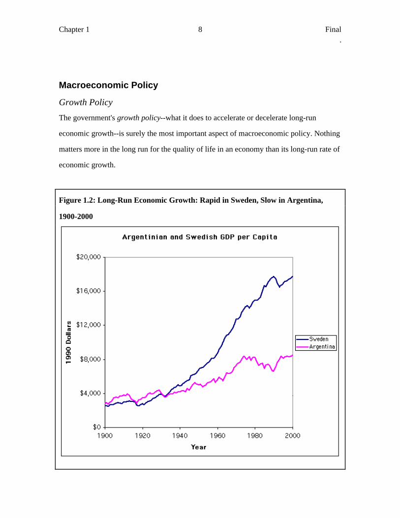
Figure 1.2: Long-Run Economic Growth: Rapid in Sweden, Slow in Argentina,
1900-2000
Chapter 1 9 Final.
Figure Legend: At the start of the twentieth century, Argentina was richer--and
seen as having a brighter future--than Sweden. But economic policies that were
mostly bad for long-run growth left Argentina far behind Sweden.
Source: Angus Maddison (1995), Monitoring the World Economy (Paris: OECD)
(as updated by the author).
Think of a country like Argentina which was once one of the most prosperous nations in
the world. In 1929, for example, Argentina was fifth in the world in the number of
automobiles per capita. Yet today Argentina is classified as a "developing" country, and
as figure 1.2 shows has fallen far behind rich developed industrial economies like
Sweden. Why? Destructive economic policies have retarded economic growth. Today
Argentines are richer than their predecessors back at the beginning of the twentieth
century, but they are not nearly as well off as they might have been had Argentinian
economic policies been as good and Argentinian economic growth as fast as in Sweden.
In Scandinavian countries like Norway and Sweden, where throughout the twentieth
century economic policies have been supportive of growth, the past hundred years have
led to extraordinary prosperity. Today economic output per person in Scandinavia is
among the highest in the world. According to semi-official estimates, Scandinavians
today are more than six times as wealthy as their predecessors back at the start of the
twentieth century.
Chapter 1 10 Final.
In the long run, nothing a government can do does more good for the economy than to
adopt good policies for economic growth.
Stabilization Policy
The second major branch of macroeconomic policy is the government's stabilization
policy. History does not show a steady, stable, smooth upward trend toward higher
production and employment. Typically, levels of production and employment fluctuate
above and below long-run growth trends. Production can easily rise several percentage
points above the long-run trend, or fall five percentage points or more below the trend
(see figure 1.3). Unemployment can fall so low that businesses become desperate for
workers and will spend much time and money training them. Or it can rise to ten percent
of the labor force in a deep recession, as it did in 1982.
Such fluctuations in production and employment are commonly referred to as business
cycles. Periods in which production grows and unemployment falls are called booms, or
macroeconomic expansions. Periods in which production falls and unemployment rises
are called recessions, or worse, depressions. Booms are to be welcomed; recessions are to
be feared.
Today's governments have powerful abilities to improve economic growth and to smooth
out the business cycle by diminishing the depth of recessions and depressions. Good
macroeconomic policy can make almost everyone's life better; bad macroeconomic
policy can make almost everyone's life much worse (see Box 1.2). For example, policy
makers' reliance on the gold standard as the international monetary system during the

Chapter 1 11 Final.
Great Depression was the source of macroeconomic catastrophe and human misery. Thus
the stakes that are at risk in the study of macroeconomics are high.
Business cycle fluctuations are felt not only in production and employment but also in the
overall level of prices. Booms usually bring inflation, orrising prices. Recessions bring
either a slowdown in the rate of inflation, or "disinflation" as it is called, or an absolute
decline in the price level, called deflation. Interest rates, the level of the stock market, and
other economic variables also rise and fall with the principal fluctuations of the business
cycle.
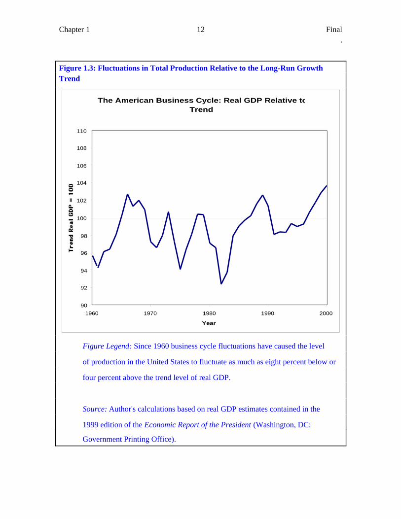
Chapter 1 12 Final.
Figure 1.3: Fluctuations in Total Production Relative to the Long-Run GrowthTrend
The American Business Cycle: Real GDP Relative to Trend
90
92
94
96
98
100
102
104
106
108
110
1960 1970 1980 1990 2000
Year
Figure Legend: Since 1960 business cycle fluctuations have caused the level
of production in the United States to fluctuate as much as eight percent below or
four percent above the trend level of real GDP.
Source: Author's calculations based on real GDP estimates contained in the
1999 edition of the Economic Report of the President (Washington, DC:
Government Printing Office).
Chapter 1 13 Final.
Box 1.2-- Macroeconomic Policy and Your Quality of Life
At the end of 1982 the U.S. macroeconomy was in the worst shape since the Great
Depression. The unemployment rate was more than ten percent. In an average week in
1983, some 10.7 million Americans were unemployed--actively seeking work, but unable
to find a job that seemed worth taking. That year the average unemployed American had
already been unemployed for more than twenty weeks. The average household income in
the United States was eight percent below its long-run trend.
By contrast, at the end of 2000 U.S. unemployment was just four percent, and average
household income was four percent above trend. In which year would you rather be
trying to find a job?
Bad macroeconomic policy makes years like 1982 and 1983 much more common than
years like 1999 and 2000. Though good macroeconomic policy cannot maintain the
degree of relative prosperity seen in 2000 indefinitely, it can all but eliminate the
prospect of years like 1982 and 1983.
Macroeconomics Versus Microeconomics
By itself macroeconomics is only half of economics. For more than half a century
economics has been divided into two branches, macroeconomics and microeconomics.
Macroeconomists examine the economy in the large, focusing on feedback from one
component of the economy to another and studying the total level of production and
Chapter 1 14 Final.
employment. In contrast, microeconomics, which was probably the subject of your last
economics course, deals with the economy in the small.
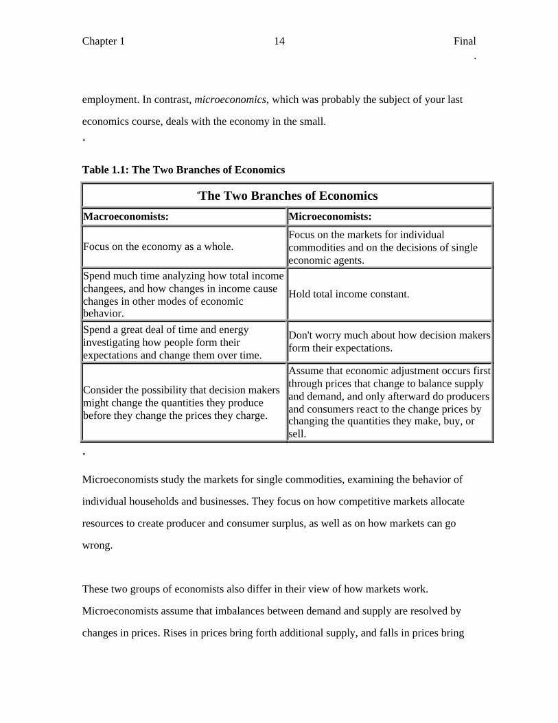
Table 1.1: The Two Branches of Economics
The Two Branches of Economics
Macroeconomists: Microeconomists:
Focus on the economy as a whole.Focus on the markets for individualcommodities and on the decisions of singleeconomic agents.
Spend much time analyzing how total incomechangees, and how changes in income causechanges in other modes of economicbehavior.
Hold total income constant.
Spend a great deal of time and energyinvestigating how people form theirexpectations and change them over time.
Don't worry much about how decision makersform their expectations.
Consider the possibility that decision makersmight change the quantities they producebefore they change the prices they charge.
Assume that economic adjustment occurs firstthrough prices that change to balance supplyand demand, and only afterward do producersand consumers react to the change prices bychanging the quantities they make, buy, orsell.
Microeconomists study the markets for single commodities, examining the behavior of
individual households and businesses. They focus on how competitive markets allocate
resources to create producer and consumer surplus, as well as on how markets can go
wrong.
These two groups of economists also differ in their view of how markets work.
Microeconomists assume that imbalances between demand and supply are resolved by
changes in prices. Rises in prices bring forth additional supply, and falls in prices bring
Chapter 1 15 Final.
forth additional demand, until supply and demand are once again in balance.
Macroeconomists consider the possibility that imbalances between supply and demand
can be resolved by changes in quantities rather than in prices. That is, businesses may be
slow to change the prices they charge, preferring instead to expand or contract production
until supply balances demand. Table 1.1 summarizes these differences in approach.
In every generation, economists attempt to integrate microeconomics and
macroeconomics by providing "microfoundations" for the macroeconomic topics of
inflation, the business cycle, and long-run growth. But no one believes that the bridge
between microeconomics and macroeconomics has yet been soundly built. Economists
are divided roughly evenly between those who think that the failure to successfully
integrate the two branches of microeconomics and macroeconomics is a flaw that
urgently needs to be corrected, and those who think it is a regrettable but minor
annoyance. Thus less knowledge may carry over from microeconomics to
macroeconomics than one might expect or hope. Be careful in trying to apply the
principles and conclusions of microeconomics to macroeconomic questions--and vice
versa.
1.2 Tracking the Macroeconomy
Economic Statistics and Economic Activity
Macroeconomics could not exist without the economic statistics that are systematically
collected and disseminated by governments. Estimates of the value and composition of
Chapter 1 16 Final.
economic activity, principally those contained in the so-called National Income and
Product Accounts [NIPA] reported by the U.S. Commerce Department's Bureau of
Economic Analysis, are the fundamental data of macroeconomics. We cannot try to
explain fluctuations in economic activity unless we know what those fluctuations are.
But what is "economic activity"?
Whenever you work for someone and get paid, that is economic activity. Whenever you
buy something at a store, that is economic activity. Whenever the government taxes you
and spends its money to build a bridge, that is economic activity. In general, if a flow of
money is involved in a transaction, economists will count that transaction as "economic"
activity. Overall, "economic activity" is the pattern of transactions in which things of real
useful value--resources, labor, goods, and services--are created, transformed, and
exchanged. If a transaction does not involve something of useful value being exchanged
for money, odds are that NIPA will not count it as part of "economic activity."
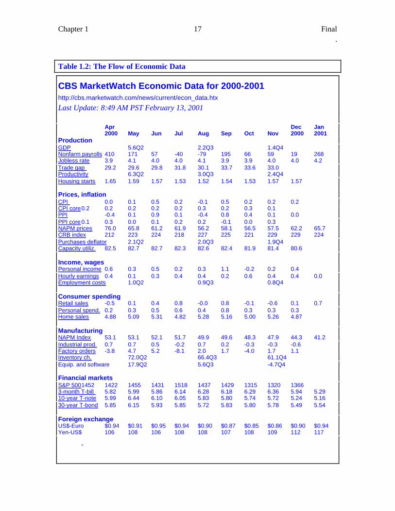
In the United States, individual economic statistics are released month-by-month and
quarter-by-quarter, a "quarter" being a three-month period: a quarter of a year. Thus you
will often hear economists and other analysts talk about the "change in inventories in the
second quarter." Table 1.2 shows a sample of the kinds of economic data that economists,
politicians, and others including investors in the stock and bond markets use to assess the
course of the economy. The sheer number of statistics is confusing at first glance, but all
the statistics are either (i) direct measures of six key economic indicators that together tell
most of the story, or (ii) primarily useful as partial forecasts of or as factors that help
determine the six key indicators of economic activity.
Chapter 1 17 Final.
Table 1.2: The Flow of Economic Data
CBS MarketWatch Economic Data for 2000-2001http://cbs.marketwatch.com/news/current/econ_data.htx
Last Update: 8:49 AM PST February 13, 2001
Apr Dec Jan2000 May Jun Jul Aug Sep Oct Nov 2000 2001
ProductionGDP 5.6Q2 2.2Q3 1.4Q4Nonfarm payrolls 410 171 57 -40 -79 195 66 59 19 268Jobless rate 3.9 4.1 4.0 4.0 4.1 3.9 3.9 4.0 4.0 4.2Trade gap 29.2 29.6 29.8 31.8 30.1 33.7 33.6 33.0Productivity 6.3Q2 3.0Q3 2.4Q4Housing starts 1.65 1.59 1.57 1.53 1.52 1.54 1.53 1.57 1.57
Prices, inflationCPI 0.0 0.1 0.5 0.2 -0.1 0.5 0.2 0.2 0.2CPI core0.2 0.2 0.2 0.2 0.2 0.3 0.2 0.3 0.1PPI -0.4 0.1 0.9 0.1 -0.4 0.8 0.4 0.1 0.0PPI core 0.1 0.3 0.0 0.1 0.2 0.2 -0.1 0.0 0.3NAPM prices 76.0 65.8 61.2 61.9 56.2 58.1 56.5 57.5 62.2 65.7CRB index 212 223 224 218 227 225 221 229 229 224Purchases deflator 2.1Q2 2.0Q3 1.9Q4Capacity utiliz. 82.5 82.7 82.7 82.3 82.6 82.4 81.9 81.4 80.6
Income, wagesPersonal income 0.6 0.3 0.5 0.2 0.3 1.1 -0.2 0.2 0.4Hourly earnings 0.4 0.1 0.3 0.4 0.4 0.2 0.6 0.4 0.4 0.0Employment costs 1.0Q2 0.9Q3 0.8Q4
Consumer spendingRetail sales -0.5 0.1 0.4 0.8 -0.0 0.8 -0.1 -0.6 0.1 0.7Personal spend. 0.2 0.3 0.5 0.6 0.4 0.8 0.3 0.3 0.3Home sales 4.88 5.09 5.31 4.82 5.28 5.16 5.00 5.26 4.87
ManufacturingNAPM Index 53.1 53.1 52.1 51.7 49.9 49.6 48.3 47.9 44.3 41.2Industrial prod. 0.7 0.7 0.5 -0.2 0.7 0.2 -0.3 -0.3 -0.6Factory orders -3.8 4.7 5.2 -8.1 2.0 1.7 -4.0 1.7 1.1Inventory ch. 72.0Q2 66.4Q3 61.1Q4Equip. and software 17.9Q2 5.6Q3 -4.7Q4
Financial marketsS&P 5001452 1422 1455 1431 1518 1437 1429 1315 1320 13663-month T-bill 5.82 5.99 5.86 6.14 6.28 6.18 6.29 6.36 5.94 5.2910-year T-note 5.99 6.44 6.10 6.05 5.83 5.80 5.74 5.72 5.24 5.1630-year T-bond 5.85 6.15 5.93 5.85 5.72 5.83 5.80 5.78 5.49 5.54
Foreign exchangeUS$-Euro $0.94 $0.91 $0.95 $0.94 $0.90 $0.87 $0.85 $0.86 $0.90 $0.94Yen-US$ 106 108 106 108 108 107 108 109 112 117

Chapter 1 18 Final.
Figure Legend: A selection of recent economic data. Most of these data are
reported monthly. A few series are reported quarterly--that is, they are calculated
four times a year only, once for the January-March period, once for April-June,
once for July-September, and once for September-December.
For a detailed description and analysis of what all these numbers mean, consult
the Glossary.
Source: CBS Marketwatch: Recent Economic Data:
http://cbs.marketwatch.com/news/current/econ_data.htx
Six Key Variables
You can get a good idea of the pulse of recent economic activity by simply looking at the
six key economic variables. Together they summarize the state of the macroeconomy. If
you want to be able to say more than "the economy is good," or "the economy is not so
good," you need to understand and be able to analyze these six variables
These six key indicators are:
• Real Gross Domestic Product
• The unemployment rate
• The inflation rate
• The interest rate
• The level of the stock market
• The exchange rate.
Chapter 1 19 Final.
The first two are the most important: they are directly and immediately connected to
people's material well-being. The other four are indicators and controls that are not
directly and immediately connected to people's current material well-being, but which
profoundly influence the economy's direction. Let's look at each of these indicators more
closely.
Real GDP
The first key indicator is the level of real Gross Domestic Product, called "real GDP" or
often just "GDP" for short. "Real" means that this measure corrects for changes in the
overall level of prices. If total spending doubles because the average level of prices
doubles but the total flow of commodities does not change, then real GDP does not
change. Economic variables are either "real"--that is, they have been adjust for changes in
the price level--or "nominal"--that is, they have not been adjusted for changes in the price
level. "Gross" means that this measure includes the replacement of worn-out and obsolete
equipment and structures as well as completely new invsetment. ("Gross" measures
contrast with "net" measures, which include only investments that add to the capital
stock. "Net" measures are better than gross measures, but the information needed to
construct them is nor reliable.)
"Domestic" means that this measure counts economic activity that happens in the United
States, whether or not the workers are legal residents and whether or not the factories are
owned by American companies. ("Domestic" measures contrast with "National"
measures which count all the economic activity conducted by U.S. citizens are permanent
residents and by the companies they own.) Finally, "product" means that real GDP
Chapter 1 20 Final.
represents the production of final goods and services. It includes both consumption goods
(things that consumers buy, take home or take out, and consume) and investment goods
(things like machine tools, buildings, highways, and bridges, that boost the country's
capital stock and productive capacity). It also includes government purchases: things that
the government (acting as our collective agent) buys and uses.
Real GDP divided by the number of workers in the economy is the most frequently used
summary index of the economy (see Box 1.3). It is a measure of how well the economy
produces goods and services that people find useful--the necessities, conveniences, and
luxuries of life. It is, however, a flawed and imperfect index. It says nothing, for instance,
about the relative distribution of the nation's economic product. And because it measures
market prices, not user satisfaction, it is an imperfect measure of material well-being.
Nevertheless real GDP per worker remains the best readily-available economic index.
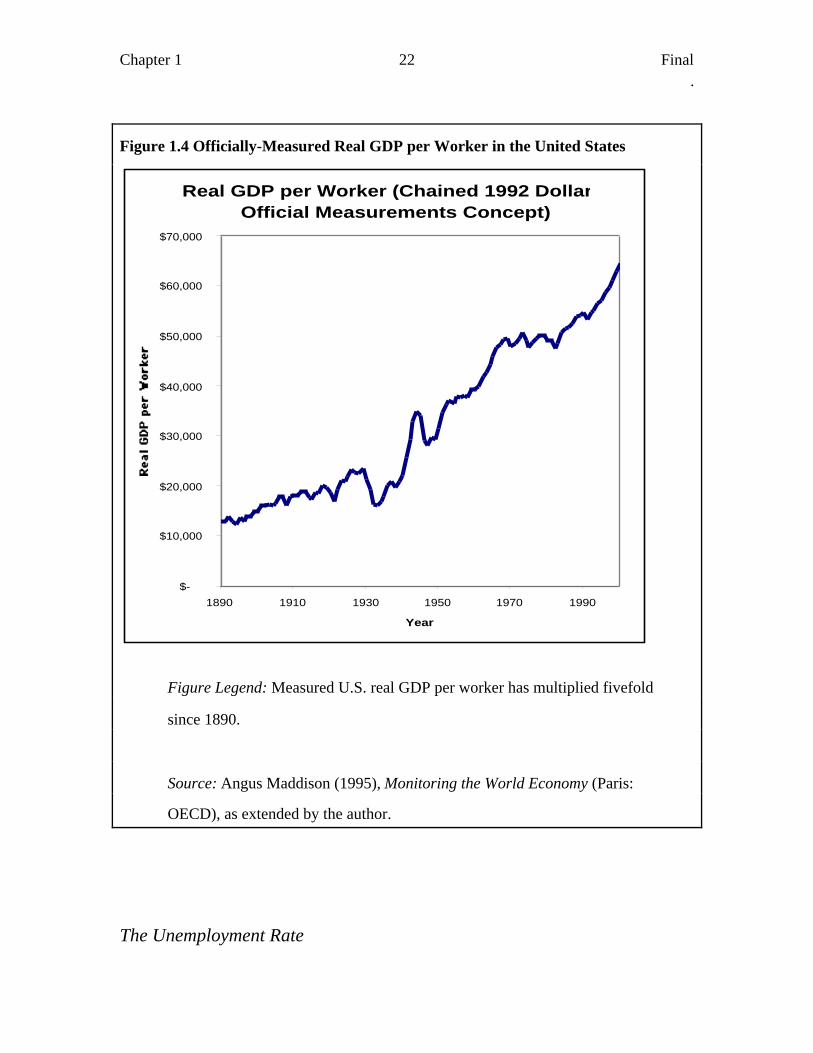
Box 1.3-- U.S. Real GDP per Worker
In the year 2000, calculated using 1992 prices, officially-measured U.S. real GDP per
worker--the total value of all final goods and services produced in the United States,
divided by the number of workers in the labor force--reached $65,000. The measured
productivity of the average American worker had quintupled since 1890, when the
standard estimate of 1992-price real GDP per worker was some $13,000. Amazingly, this
upward leap in economic well-being was accomplished in a little over three generations.
Figure 1.4 shows this upward trend in real GDP per worker. Despite temporary setbacks
in recessions and depressions--of which the Great Depression of the 1930s--was by far
the largest--the principal event of the twentieth century was this quintupling of measured
Chapter 1 21 Final.
real GDP per worker. Other macroeconomic events visible in the figure include the
World War II boom, the 1974-1975 and the 1980-1983 major recessions, the 1990-1991
minor recession, and the two-decade long period of stagnation from the early 1970s to the
early 1990s--a period that saw the 1973 and 1979 sharp oil price increases by OPEC, and
the large investment-reducing government budget deficits of the 1990s.
Note that this figure says nothing at all about how economic growth was distributed. In
fact, the years between 1930 and 1970 saw the middle and working classes diminish the
relative income gap between themselves and the rich. The years between 1970 and the
present have see this gap open wider once again.
Chapter 1 22 Final.
Figure 1.4 Officially-Measured Real GDP per Worker in the United States
Real GDP per Worker (Chained 1992 Dollars; Official Measurements Concept)
$-
$10,000
$20,000
$30,000
$40,000
$50,000
$60,000
$70,000
1890 1910 1930 1950 1970 1990
Year
Figure Legend: Measured U.S. real GDP per worker has multiplied fivefold
since 1890.
Source: Angus Maddison (1995), Monitoring the World Economy (Paris:
OECD), as extended by the author.
The Unemployment Rate
Chapter 1 23 Final.
The second key quantity is the unemployment rate. The unemployed are people who want
to work and who are looking actively looking for jobs, but who have not yet found one
(or have not yet found one that they find attractive enough to take rather than continue to
look for a still better job). The unemployment rate is equal to the number of unemployed
people divided by the total labor force, which is just the sum of the number of
unemployed people and the number of people who have jobs. The U.S. Labor
Department's Bureau of Labor Statistics conducts the Current Population Survey: a
random survey of America's households, every month. The estimated number of
unemployed workers obtained from the survey is then divided by the estimated total labor
force, also obtained from the survey. The result is that month's unemployment rate. It is
released to the public on the first Friday of the next month.
Most people consider unemployment to be a bad thing, and it usually is. Yet it is
important to notice that an economy with no unemployment at all would probably be a
badly-working economy. Just as an economy needs inventories of goods--goods in
transit, goods in process, goods in warehouses and sitting on store shelves--in order to
function smoothly, it needs "inventories" of jobs-looking-for-workers ("vacancies") and
workers-looking-for-jobs ("the unemployed"). An economy in which each business
grabbed the first person who walked through the door to fill a newly-open job and in
which each worker took the first job offered would be a less productive economy.
Workers should be somewhat choosy about what jobs they take. They should decline jobs
when they think that "this job pays too little," or "this job would be too unpleasant."
Likewise, employers should be choosy about which workers they hire. Such frictional
unemployment is an inevitable part of the process that makes good matches between
workers and firms--matches that pair qualified workers with jobs that use their
qualifications.
Chapter 1 24 Final.
During recessions and depressions, however, unemployment is definitely not "frictional."
In these downturns in the business cycle the unemployment rate can rise far far above the
level of a normal and healthy process of job search. The market economy breaks down,
failing match workers willing and able to work with businesses that could put their skills
and labor-power to making useful goods and services. Economists call this type of
unemployment cyclical unemployment. In the United States in the Great Depression the
unemployment rose to 25%. In Germany during the Great Depression the unemployment
rate rose to 33%.
When the unemployment rate is high, the market economy is not functioning well. The
unemployment rate is the best indicator of how well the economy is doing relative to its
productive potential.
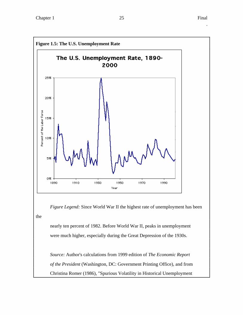
Box 1.4--The U.S. Unemployment Rate in the Twentieth Century
In the twentieth century the U.S. unemployment rate dipped as low as 1.5 percent during
World War II and as high as 25 percent during the Great Depression, the principal
macroeconomic catastrophe of the past century. No other recession or depression in the
nation's history, not even the depression of the early 1890s, came close to the Great
Depression's devastating impact (see Figure 1.5).
Chapter 1 25 Final.
Figure 1.5: The U.S. Unemployment Rate
Figure Legend: Since World War II the highest rate of unemployment has been
the
nearly ten percent of 1982. Before World War II, peaks in unemployment
were much higher, especially during the Great Depression of the 1930s.
Source: Author's calculations from 1999 edition of The Economic Report
of the President (Washington, DC: Government Printing Office), and from
Christina Romer (1986), "Spurious Volatility in Historical Unemployment
Chapter 1 26 Final.
Estimates," Journal of Political Economy.
Since World War II, the U.S. unemployment rate has fluctuated between 3 and 10
percent, with the highest rates occurring in the decades of the 1970s and 1980s.
The Inflation Rate
A third key economic indicator is the inflation rate, a measure of how fast the overall
price level is rising. If the inflation rate this year is five percent, that means that in
general things cost five percent more this year than they cost last year in money terms, in
terms of the symbols printed on dollar bills. A very high inflation rate--more than 20
percent a month, say--can cause massive economic destruction, as the price system
breaks down and the possibility of using profit-and-loss calculations to make rational
business decisions vanishes. Such episodes of hyperinflation are among the worst
economic disasters that can befall an economy. But not since the Revolutionary War has
the U.S. experienced hyperinflation. Box 1.5 tracks the inflation rate in the United States
over the past century.
Strangely, moderate inflation rates--a little more than 10 percent a year, say--are highly
unsettling to consumers and business managers. Moderate inflation should not seriously
compromise consumers', investors', and managers' ability to determine the best use of
their financial resources or to calculate profitability. Yet all these groups are strongly
averse to it. Politicians in the industrialized economies have discovered that if they fail to
preside over low and stable inflation rates then they are likely to lose the next election.
Chapter 1 27 Final.
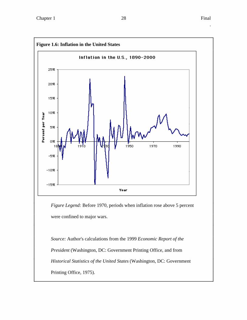
Box 1.5-- U.S. Inflation Rates in the Twentieth Century
In the United States in the twentieth century significant peaks of inflation occurred during
World Wars I and II, when overall rates of price increase peaked at more than twenty
percent per year (see Figure 1.6). Before World War II, deep recessions like the Great
Depression of the 1930s were accompanied by deflation: a decline in the level of overall
prices that bankrupted businesses and banks, exacerbating the fall in output and
employment.
Chapter 1 28 Final.
Figure 1.6: Inflation in the United States
Figure Legend: Before 1970, periods when inflation rose above 5 percent
were confined to major wars.
Source: Author's calculations from the 1999 Economic Report of the
President (Washington, DC: Government Printing Office, and from
Historical Statistics of the United States (Washington, DC: Government
Printing Office, 1975).
Chapter 1 29 Final.
Since World War II there has been only one single year--in the late 1940s--during which
the price level declined. Otherwise, there has been inflation. Post-WWII inflation has
come in two varieties: the "creeping" inflation of the 1950s, early and mid 1960s, and
1990s, too small and slow for anyone to pay much attention to it; and the "trotting"
inflation of the late 1960s, 1970s, and 1980s--too high to ignore, and too tempting a
political football for politicians to resist blaming the current government.
The steep decline in inflation that occurred in the early 1980s is called the "Volcker
disinflation," after then-Federal Reserve Chair Paul Volcker. Alarmed by the accelerating
inflation of the late 1970s and early 1980s, Volcker decided to raise interest rates in order
to decrease aggregate demand. In doing so he risked a deep recession, which came in
1982-1983. But his action did stop the rise in inflation and reduce it back to the
"creeping" range.
The Interest Rate
The fourth key economic indicator is the interest rate. Though economists speak of "the"
interest rate, there are actually many different interest rates applying to loans of different
durations and different degrees of risk. (After all, the person or business entity to whom
you lend your money may be unable to pay it back: that is a risk you accept when you
make a loan.) The different interest rates often move up or down together so that
economists speak of the interest rate, referring to the entire complex of different rates.
But interest rates do not move in concert all the time. The causes of variations in the yield
Chapter 1 30 Final.
curve, which describes the pattern of interest rates, are an important part of
macroeconomics.
The interest rate is important because it governs the redistribution of purchasing power
across time. Those people or business enterprises who think they can make good use of
additional financial resources borrow, promising to return the purchasing power they use
today with interest in the future. Those business enterprises or people who have no
immediate use for their financial resources lend, hoping to profit when the borrower
returns the borrowed sum--what financiers call the principal--with interest.
When economists think about interest rates, they almost always prefer to focus on the
real interest rate rather than the nominal interest rate. The nominal interest rate is the
interest rate in terms of money--for example, how many dollars' worth of interest a
borrower must pay to borrow a given sum of money for one year. The real interest rate is
the interest rate in terms of goods and services--for example, how much purchasing
power over goods and services a borrower must pay in order to borrow a given amount of
purchasing power for one year. The difference between the two is that nominal interest
rates do not take proper account of the effect of inflation; real interest rates do.
Whenever interest rates are low--that is, when money is "cheap"--investment tends to be
high, because businesses find that a wide range of possible investments will generate
enough cash to pay the interest on borrowed money, repay the principal of the loan, and
still produce a profit. Whenever interest rates are high--that is, when money is "dear"--
investment tends to be low, because businesses find that most possible investments will
not generate enough cash flow to repay the principal and the high interest. Box 1.6 shows
changes in real interest rates in the United States since 1960.
Chapter 1 31 Final.
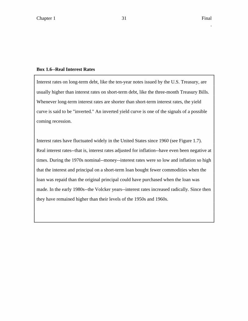
Box 1.6--Real Interest Rates
Interest rates on long-term debt, like the ten-year notes issued by the U.S. Treasury, are
usually higher than interest rates on short-term debt, like the three-month Treasury Bills.
Whenever long-term interest rates are shorter than short-term interest rates, the yield
curve is said to be "inverted." An inverted yield curve is one of the signals of a possible
coming recession.
Interest rates have fluctuated widely in the United States since 1960 (see Figure 1.7).
Real interest rates--that is, interest rates adjusted for inflation--have even been negative at
times. During the 1970s nominal--money--interest rates were so low and inflation so high
that the interest and principal on a short-term loan bought fewer commodities when the
loan was repaid than the original principal could have purchased when the loan was
made. In the early 1980s--the Volcker years--interest rates increased radically. Since then
they have remained higher than their levels of the 1950s and 1960s.
Chapter 1 32 Final.
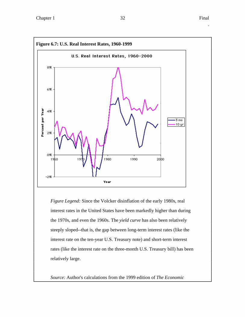
Figure 6.7: U.S. Real Interest Rates, 1960-1999
Figure Legend: Since the Volcker disinflation of the early 1980s, real
interest rates in the United States have been markedly higher than during
the 1970s, and even the 1960s. The yield curve has also been relatively
steeply sloped--that is, the gap between long-term interest rates (like the
interest rate on the ten-year U.S. Treasury note) and short-term interest
rates (like the interest rate on the three-month U.S. Treasury bill) has been
relatively large.
Source: Author's calculations from the 1999 edition of The Economic
Chapter 1 33 Final.
Report of the President (Washington, DC: Government Printing Office),
and from Historical Statistics of the United States (Washington, DC:
Government Printing Office, 1975).
The Stock Market
The level of the stock market is the key economic indicator you hear about most often--
you hear about it every single day unless you try hard to avoid the news. The level of the
stock market is an index of expectations for the future. When the stock market is high,
investors expect economic growth to be rapid, profits to be high, and unemployment to be
relatively low. (Note, however, that there is an element of tail-chasing in the stock
market: perhaps it would be more accurate to say that the stock market is high when
average opinion expects that average opinion will expect that future economic growth
will be rapid.) Conversely, when the stock market is low, it is because investors expect
the economic future to be relatvely gloomy.
At times--like the end of the 1960s, or the end of the 1990s-- the stock market appears
significantly overvalued compared to its standard historical patterns. During such
episodes investors are implicitly forecasting a major boom and continued rapid
productivity growth. If their forecasts turn out to be wrong, these investors will be
severely disappointed with their stock market investments. Box 1.7 shows the course of
the U.S. stock market over the past century.
Box 1.7-- The Stock Market
Chapter 1 34 Final.
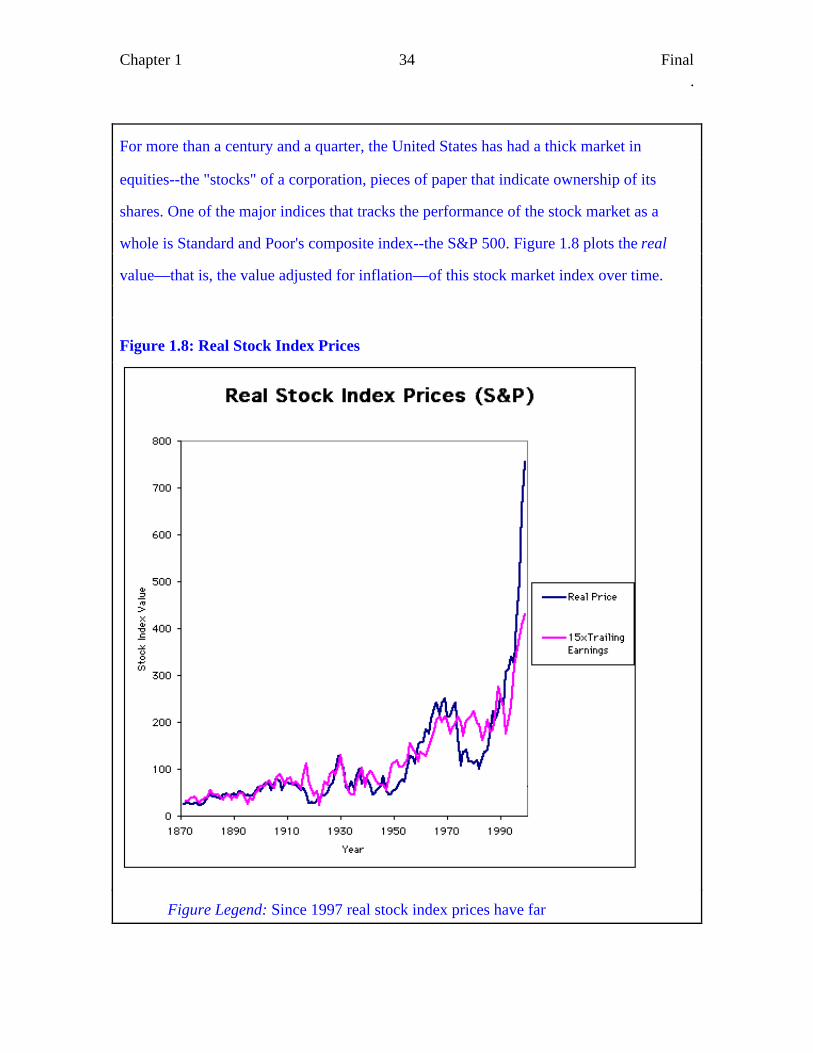
For more than a century and a quarter, the United States has had a thick market in
equities--the "stocks" of a corporation, pieces of paper that indicate ownership of its
shares. One of the major indices that tracks the performance of the stock market as a
whole is Standard and Poor's composite index--the S&P 500. Figure 1.8 plots the real
value—that is, the value adjusted for inflation—of this stock market index over time.
Figure 1.8: Real Stock Index Prices
Figure Legend: Since 1997 real stock index prices have far
Chapter 1 35 Final.
exceeded their standard, conventional valuation of fifteen times earnings.
Economists differ over whether this phenomenon is due to (a) an
irrational speculative mania, (b) an increased tolerance for risk, or (c)
expectations of rapid future economic growth on the part of investors.
Source: Author's calculations from data in Robert Shiller (1987), Market
Volatility (Cambridge: MIT Press), as subsequently extended by Shiller.
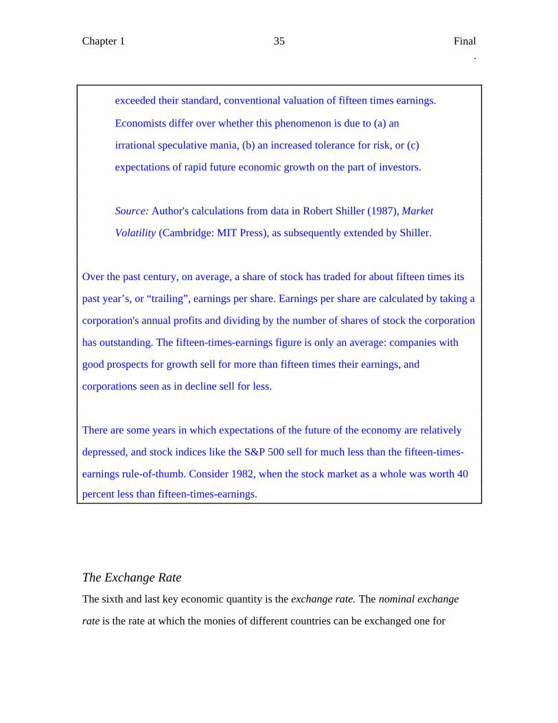
Over the past century, on average, a share of stock has traded for about fifteen times its
past year’s, or “trailing”, earnings per share. Earnings per share are calculated by taking a
corporation's annual profits and dividing by the number of shares of stock the corporation
has outstanding. The fifteen-times-earnings figure is only an average: companies with
good prospects for growth sell for more than fifteen times their earnings, and
corporations seen as in decline sell for less.
There are some years in which expectations of the future of the economy are relatively
depressed, and stock indices like the S&P 500 sell for much less than the fifteen-times-
earnings rule-of-thumb. Consider 1982, when the stock market as a whole was worth 40
percent less than fifteen-times-earnings.
The Exchange Rate
The sixth and last key economic quantity is the exchange rate. The nominal exchange
rate is the rate at which the monies of different countries can be exchanged one for
Chapter 1 36 Final.
another. The real exchange rate is the rate at which the goods and services produced in
different countries can be exchanged one for another.
The exchange rate governs the terms on which international trade and investment take
place. When the domestic currency is appreciated, its value in terms of other currencies
is high. Foreign-produced goods are relatively cheap for domestic buyers, but domestic-
made goods are relatively expensive for foreigners. In these circumstances imports are
likely to be high; exports are likely to be low. When the domestic currency is
depreciated, the opposite is the case. Domestically-made goods are cheap to foreign
buyers. Thus exports are likely to be high. But domestic consumers' and investors' power
to purchase foreign-made goods is limited. Thus imports are likely to be low. Box 1.8
details the effects of changes in the U.S. exchange rate since 1977.
Box 1.8--The Exchange Rate
The terms on which people in one country can buy goods and services made in other
countries--and sell the goods and services they make themselves--are summarized in the
exchange rate. The nominal exchange rate tells how many units of foreign currency can
be bought with one unit of the domestic currency: it is the value of a foreign currency.
The real exchange rate adjusts for differences in the rate of inflation between countries.
Thus it measures the relative price of tradeable goods: how much in the way of foreign-
produced goods can be bought with one unit of domestically produced goods.
Chapter 1 37 Final.
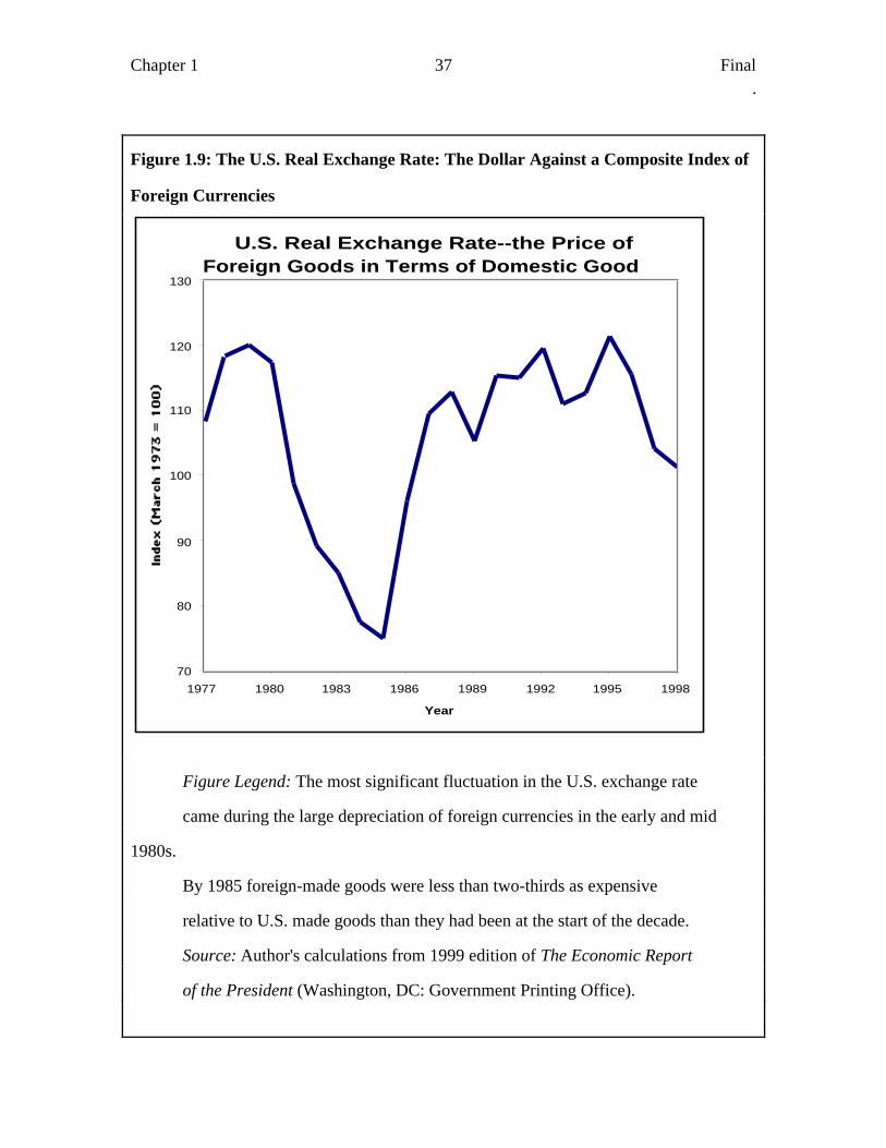
Figure 1.9: The U.S. Real Exchange Rate: The Dollar Against a Composite Index of
Foreign Currencies
U.S. Real Exchange Rate--the Price of Foreign Goods in Terms of Domestic Goods
70
80
90
100
110
120
130
1977 1980 1983 1986 1989 1992 1995 1998
Year
Figure Legend: The most significant fluctuation in the U.S. exchange rate
came during the large depreciation of foreign currencies in the early and mid
1980s.
By 1985 foreign-made goods were less than two-thirds as expensive
relative to U.S. made goods than they had been at the start of the decade.
Source: Author's calculations from 1999 edition of The Economic Report
of the President (Washington, DC: Government Printing Office).
Chapter 1 38 Final.
Before the early 1970s, the U.S. exchange rate was fixed vis-a-vis other major currencies
in the Bretton Woods System. The U.S. Treasury stood ready to buy or sell dollars in
exchange for other currencies at fixed parities determined by each country's posted
valuation of its currency in terms of gold.
Since the early 1970s the U.S. exchange rate has been floating--free to move up or down
in response to the market forces of supply and demand (see Figure 1.9). When U.S.
interest rates have been relatively high compared to other countries--as in the early
1980s--the dollar has appreciated. In such a case the dollar will have become much more
valuable, as many people have tried to invest in America to capture the high interest
rates. We then say that the value of the exchange rate is relatively low. The exchange rate
is defined as the value (in terms of dollars) of foreign currency: when the relative value of
the dollar rises, the value in dollars of foreign currency falls.
When U.S. interest rates fall relative to those in other countries, the dollar tends to
depreciate: to fall in value so that U.S. goods are cheap to buy and easy to sell. When the
dollar’s value is low and the dollar has depreciated, the exchange rate—the value in
dollars of foreign currency—will be relatively high.
Real GDP, the unemployment rate, the inflation, the interest rate, the stock market, and
the exchange rate--these are the six key economic indicators. Know the values of these
six key variables in context--both their relative levels today and their recent trends--and
you have a remarkably complete picture of the current state of the macroeconomy.
Chapter 1 39 Final.
1.3 The Current Macroeconomic Situation
The United States
As of the winter of 2001, the United States macroeconomy teetered on the brink of a
recession. The consensus of observers of the economy was that the Federal Reserve had
overdone it and raised interest rates too far too fast in late 1999 and 2000. Thus by the
start of 2001 economic growth in the United States had slowed to a very weak pace. The
consensus forecast was that the year 2001 would see U.S. real GDP grow by no more
than 1.8%, and a recession--an absolute fall in real GDP for two quarters--was a definite
possibility.
The Federal Reserve reacted to the bad economic news over the winter of 2001 by
sharply and rapidly lowering interest rates. But Federal Reserve policies affect the
economy only with significant lags. Reductions in interest rates at the start of 2001 would
not have any noticeable effect on the economy until the very end of the year. And the tax
cuts proposed by the new President, George W. Bush, would take even longer to affect
production and employment.
As Americans contemplated the prospect of a recession, the bright spot was that the
Federal Reserve was ready and anxious to take steps to fight any slowdown. The larger
recessions of the post-World War II period had all come to pass because the Federal
Reserve was more concerned with fighting inflation than with avoiding recession. In the
winter of 2001, however, inflation continued to be less than 2 percent per year and was
not seen as a threat by anyone.
Chapter 1 40 Final.
The slowdown at the very end of 2000 had been preceded by a remarkable decade-long
economic boom. Policymakers and economists advocating the Clinton deficit-reduction
program in the early 1990s had claimed that deficit reduction would make possible a
high-investment economic expansion, which would then become a high productivity
growth expansion. Up until 1996 there had been no signs that high investment was
leading to high productivity growth. But by the late summer of 1999 productivity growth
had been strong for four years in a row. Perhaps political claims in the early 1990s that
deficit reduction would ignite a high-investment and high-productivity growth recovery
were coming true. Perhaps the U.S. economy was simply benefiting from the sudden
wave of rapid productivity growth driven by the technological revolutions in data
processing and data communications.
In the United States the strong growth in production and sales in the second half of the
1990s had pushed the unemployment rate down to a level—four percent--not seen in a
generation. A tight labor market was good news for workers: employers appeared eager
to pour resources into training them for their jobs. Yet the tight labor market and the
strong demand for employees was not showing up in strong real wage growth. Real
wages in the year up through December 1999 had grown at only 1.9 percent. On the other
hand, relatively slow nominal wage growth meant that inflation remained low as well.
This low inflation proved a puzzle to economists: practically all had confidently forecast
(using their estimates of the Phillips Curve relationship between inflation and
unemployment) that unemployment below 5 percent would surely lead to accelerating
inflation. Yet it had not done so.
Chapter 1 41 Final.
Europe and Japan
As of the winter of 2001, economic growth in the eleven countries belonging to the
European Monetary Union--and having the "euro" for their principal currency--was
slowing. Rising oil prices and rising interest rates (in large part a result of the fear on the
part of the newly-formed European Central Bank that its currency, the euro, had
depreciated too far) had reduced growth in late 2000 below what had been forecast.
There was certainly room for economic expansion in Europe. The preceding year had
seen consumer prices throughout the euro zone rise by less than 2 percent. Economic
forecasters were projecting 3 percent real GDP growth for 2001. Unfortunately, such a
rate of growth would have little or no effect at reducing European unemployment, which
remained stuck near 10 percent. The challenge for European policy remained one of
avoiding rises in inflation while attempting to reduce western Europe's distressingly high
and stubborn rate of unemployment.
Japan ended 2000 with an annual real GDP growth rate of 1.8%. This is an astonishingly
low growth rate given the large amount of unused capacity in the Japanese economy and
the extraordinarily low levels of nominal short-term interest rates in Japan. One reason
for the low growth rate is that people are unsure whether prices have further to fall: Japan
is actually undergoing deflation, with prices falling by 0.7 percent in 2000. Real GDP
growth in Japan for 2001 is projected to be only 1.4%, certainly less than the rate of
growth of potential output.
Perhaps it is time for the Japanese government to pursue a policy of thorough-going
inflation to boost demand that has been extremely sluggish for nearly a decade. But the
Chapter 1 42 Final.
conventional wisdom is that Japanese demand and production is unlikely to pick up until
ongoing "structural" problems--in particular the fear of lenders that those who want to
borrow from them are really bankrupt--are resolved. Requiring businesses to declare the
true value of their real estate holdings is commonly pointed to as the key blockage to
investment, higher demand, and economic recovery.
As of the winter of 2001, the financial crisis in East Asia had been over for nearly two
years. The panic that started in 1997 on the part of investors in New York, Frankfurt,
London, and Tokyo, and the consequent withdrawal of their money from emerging
market economies imposed very high costs: massive bankruptcies, high interest rates,
increases in unemployment, falls in production. However, foreign investors appear to
have regained confidence in East Asian economies. Recovery and growth is rapid
throughout the region, save in Indonesia.
1.4 Chapter Summary
Main Points
1. Macroeconomics is the study of the economy in the large--the determination of the
economy-wide levels of production, of employment and unemployment, and inflation or
deflation.
2. There are three key reasons to study macroeconomics: first, to gain cultural literacy;
second, to understand how economic trends affect you personally; and third, to exercise
your responsibility as a voter and citizen.
Chapter 1 43 Final.
3. The six key variables in macroeconomics are: real GDP, the unemployment rate, the
inflation rate, the interest rate, the level of the stock market, and the exchange rate.
Important Concepts
Macroeconomics
Microeconomics
Inflation
Deflation
Real GDP
Real GDP per worker
The unemployment rate
The (real) exchange rate
The interest rate
The stock market
Expansion
Recession
Depression
Analytical Exercises
Chapter 1 44 Final.
1. What are the key differences between microeconomics and macroeconomics?
2. Why are real GDP and the unemployment rate important macroeconomic variables?
3. What macroeconomic issues are in the newspaper headlines this morning? Has chapter
one of this textbook been any use in understanding them?
4. Why is the inflation rate an important macroeconomic variable?
5. Why are the interest rate and the level of the stock market important economic
variables?
6. Roughly, what was the highest level that the U.S. inflation rate reached in the twentieth
century? What was the highest peacetime unemployment rate?
7. Roughly, what was the highest peak in the U.S. unemployment rate in the twentieth
century? What was the second-highest peak in the unemployment rate?
8. Roughly much higher is the U.S. stock market today than it was back at the start of the
twentieth century?
9. Roughly how much higher is measured real GDP per worker today than it was in
1973?
Chapter 1 45 Final.
10. Count backward from 1973 by the same number of years n that separate this year
from 1973. Roughly how much higher was measured real GDP per worker in 1973 than it
was that number n years earlier?
Policy-Relevant Exercises
1. What was the rate of real GDP growth in the United States in 2000?
2. What was the rate of real GDP growth in the United States in the first half of 2001?
3. What was the latest number that the Commerce Department's Bureau of Economic
Analysis reported for real GDP growth? What period did it cover?
4. What is the current unemployment rate?
5. What is the current inflation rate? If you find more than one inflation rate listed, are
they consistent with each other?
6. What is the current level of the short-term real interest rate? Of the long-term real
interest rate? Of the short-term nominal interest rate?
7. What is the current level of the stock market? How does it compare to the level of the
stock market at the beginning of the year 2000?
Chapter 1 46 Final.
8. How does the current level of the stock market compare with the historical average,
roughly fifteen times a stock market index's trailing earnings?
9. What is the current value of the exchange rate? Is the exchange rate higher or lower
than it was at the beginning of the year 2000?
10. Has the exchange rate exhibited any extraordinary fluctuations over the past two
decades? If so, what effects do you think they had on the economy?