Introduction to Many-Valued Logics - Technische Universit¤t Dresden

Introduction to Many-Valued Logics

Bertram Fronhöfer

Faculty of Computer Science

Technische Universität Dresden

August 4, 2011

OVERVIEW

1. Modern Pioneers of 3-Valued Logic

2. Definability of Connectives

3. Non Truth Centered Semantical Concepts

4. Derivation Systems for 3-Valued Propositional Logic

5. Łukasiewicz Modalities

HISTORICAL SKETCH

“Ever since there was first a clear enunciation of the principleEvery proposition is either true or false,there have been those who questioned it.”

[Rosser & Turquette, 1952, p.10]

I Debate on Truth Values started already in Antiquity

I Modern Prehistory (around 1900): Peirce, (MacColl, Vasiliev)

I Modern Pioneers (from 1918 onwards):Łukasiewicz, Kleene, Bochvar, Post, . . . ,

I Further important developments:Zadeh and Fuzzy Logic . . .

LANDSCAPE OF MANY-VALUED LOGICS

Many-Valued Logic = logic with more than 2 truth values

Many-Valued Logic

↙ ↘

truth-functional not truth-functional

↓ |

3 |

↓ |

4 |... |

∞ ↓

↓ possibilistic logic

Fuzzy probabilistic logic

Usually, the term Many-Valued Logics refers to the left branch

2

1. Modern Pioneers of 3-Valued LogicPrelude: Classical (Two-valued) Propositional LogicHistory and Intuition of Many-Valued LogicKleene’s Strong 3-Valued LogicŁukasiewicz’s 3-Valued LogicBochvar’s Internal 3-Valued LogicBochvar’s External 3-Valued Logic


PROPOSITIONAL ALPHABET AND FORMULAS

Definition 1.1

An alphabet of propositional logic consists of

I a set R = {p1, p2, p3, . . . } of propositional variables

I the set {¬ /1, ∧ /2, ∨ /2, →/2, ↔/2 } of (standard) connectives(with indication of their arities)

I the special characters “ ( ” and “ ) ”

Definition 1.2

The set of propositional formulas is the smallest set CL with the following properties:

1. If F ∈R , then F ∈ CL (called atomic formula or atom).

2. If ◦ /1 is a unary connective, F ∈ CL , then ◦ F ∈ CL .

3. If ◦ /2 is a binary connective, F, G ∈ CL , then (F ◦ G) ∈ CL .

We usually drop an outer pair of parentheses.

CLASSICAL (TWO-VALUED) SEMANTICS

Definition 1.3

I We denote by the set W2 = {>,⊥ } of (classical) truth values

I For each connective ◦ /n we define a truth function ◦? :Wn2 →W2

Definition 1.4

A classical (propositional) interpretation I = (W2, ·I)

consists of the set W2 = {>,⊥ } of truth values and a mapping ·I : CL →W2 with:

[F]I =

◦? [G]I if F is of the form ◦ G,

([G1]I ◦? [G2]I) if F is of the form (G1 ◦ G2).

6

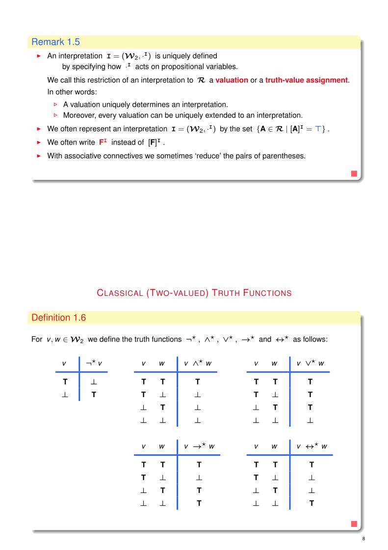
Remark 1.5I An interpretation I = (W2, ·I) is uniquely defined

by specifying how ·I acts on propositional variables.

We call this restriction of an interpretation to R a valuation or a truth-value assignment.

In other words:. A valuation uniquely determines an interpretation.. Moreover, every valuation can be uniquely extended to an interpretation.

I We often represent an interpretation I = (W2, ·I) by the set {A ∈R | [A]I = >} .

I We often write FI instead of [F]I .

I With associative connectives we sometimes ‘reduce’ the pairs of parentheses.

CLASSICAL (TWO-VALUED) TRUTH FUNCTIONS

Definition 1.6

For v ,w ∈W2 we define the truth functions ¬? , ∧? , ∨? , →? and ↔? as follows:

v ¬? v

T ⊥⊥ T

v w v ∧? w

T T T

T ⊥ ⊥⊥ T ⊥⊥ ⊥ ⊥

v w v ∨? w

T T T

T ⊥ T

⊥ T T

⊥ ⊥ ⊥

v w v →? w

T T T

T ⊥ ⊥⊥ T T

⊥ ⊥ T

v w v ↔? w

T T T

T ⊥ ⊥⊥ T ⊥⊥ ⊥ T

8

SATISFIABILITY, VALIDITY, . . .

Definition 1.7

Let F ∈ CL .

I F is called satisfiable ⇐⇒there is an interpretation I = (W2, ·I) with FI = > .

I F is called valid (or F is a tautology) ⇐⇒for all interpretations I = (W2, ·I) we have: FI = > .

I F is called falsifiable or refutable ⇐⇒there is an interpretation I = (W2, ·I) with FI = ⊥ .

I F is called unsatisfiable ⇐⇒for all interpretations I = (W2, ·I) we have: FI = ⊥ .

Two formulas F and G of classical propositional logic are equivalent ⇐⇒they have the same truth-value on each truth-value assignment.(This will be denoted by F ≡ G .)

TRUTH TABLE METHOD

Example 1.8Truth-table for the formula ¬P ∧ (Q ∨ R) (with P , Q and R in R ):

P Q R ¬ P ∧ (Q ∨ R)

T T T ⊥ T ⊥ T T T

T T ⊥ ⊥ T ⊥ T T ⊥⊥ T T T ⊥ T T T T

⊥ T ⊥ T ⊥ T T T ⊥T ⊥ T ⊥ T ⊥ ⊥ T T

T ⊥ ⊥ ⊥ T ⊥ ⊥ ⊥ ⊥⊥ ⊥ T T ⊥ T ⊥ T T

⊥ ⊥ ⊥ T ⊥ ⊥ ⊥ ⊥ ⊥

10

PRIMITIVE CONNECTIVES

Definition 1.9

We take ¬ and ∧ as primitive connectives and define the other (standard) connectives asfollows:

P ∨ Q := ¬(¬P ∧ ¬Q)

P→ Q := ¬(P ∧ ¬Q)

P↔ Q := ¬(P ∧ ¬Q) ∧ ¬(¬P ∧ Q) .

Remark 1.10These definitions are semantically correct, as can be verified, for instance, via truth tables.

P Q P ∨ Q ¬ (¬ P ∧ ¬ Q)

T T T T T T ⊥ T ⊥ ⊥ T

T ⊥ T T ⊥ T ⊥ T ⊥ T ⊥⊥ T ⊥ T T T T ⊥ ⊥ ⊥ T

⊥ ⊥ ⊥ ⊥ ⊥ ⊥ T ⊥ T T ⊥

Remark 1.11Other choices of primitive connectives are possible

I Another common (and similar) way of dividing the connectivesinto primitive and defined onesis to take ¬ and ∨ as primitive and then to introduce the others as:

P ∧ Q := ¬(¬P ∨ ¬Q)

P→ Q := ¬P ∨ Q

P↔ Q := ¬(¬P ∨ ¬Q) ∨ ¬(P ∨ Q)

I The two connectives ¬ and → can also be taken as primitive,which is a very frequent choice when axiomatizing a logic.

12

MODELS

Definition 1.12

An interpretation I = (W2, ·I) is called a model for a propositional formula F ,in symbols I |= F ,⇐⇒ FI = > .

Theorem 1.13

A propositional formula F is valid ( |= F ) ⇐⇒ ¬F is unsatisfiable.

Definition 1.14

Let G be a set of formulas.

I G is satisfiable ⇐⇒ there is an interpretation mapping each element F ∈ G to > .

I An interpretation I is called model for G , in symbols I |= G ⇐⇒I is model for all F ∈ G .

LOGICAL CONSEQUENCE

Definition 1.15

I A propositional formula F is a (propositional) consequenceof a set G of propositional formulas – in symbols G |= F ⇐⇒for every interpretation I it holds: if I |= G , then I |= F .

We also say that the set G of formulas entails the formula F .

Convention: In case of G = {G } we just write G |= F instead of {G } |= F .

I F is valid or a tautology – |= F , for short – ⇐⇒F evaluates to > under every interpretation.

I F is a contradiction ⇐⇒ F evaluates to ⊥ under every interpretation.

Theorem 1.16

I Let F, F1, . . . , Fn be propositional formulas.

{F1, . . . , Fn} |= F holds ⇐⇒ |= ((. . . (F1 ∧ F2) ∧ . . . ∧ Fn)→ F) holds.

I For formulae F and G of classical propositional holds:

F ≡ G ⇐⇒ {F } |= G and {G } |= F .

14

ARGUMENTS

Definition 1.17

I A (deductive) argument is a pair (S,F) with formula F and set S of formulas.

I The formulas in S are called premises,and the formula F is called the conclusion.

I We say that an argument is valid ⇐⇒the set consisting of its premises entails the argument’s conclusion, i.e. S |= F .

I We also say that the conclusion of a valid argument follows from the premises.

Remark 1.18The components of an argument are traditionally displayed by writing the premises, one per line,followed by a separator line and then the conclusion.

For example: P→ QP

Q

or J→ C¬ J

¬C

The first argument is valid, the second not, as can be seen with the following truth tables.

P Q P → Q P Q

T T T T T T T

T ⊥ T ⊥ ⊥ T ⊥⊥ T ⊥ T T ⊥ T

⊥ ⊥ ⊥ T ⊥ ⊥ ⊥

F G F → G ¬ F ¬ G

T T T T T ⊥ T ⊥ T

T ⊥ T ⊥ ⊥ ⊥ T T ⊥⊥ T ⊥ T T T ⊥ ⊥ T

⊥ ⊥ ⊥ T ⊥ T ⊥ T ⊥

Remark 1.19

I Law of Non-Contradiction

It is the negation of the formula A ∧ ¬A which is a contradiction in classical logic.

Consequently, ¬(A ∧ ¬A) is a tautology.

I Law of Excluded Middle

A symbolic version is F ∨ ¬F , and this is a tautology in classical logic.

Note its equivalence with the XOR version – either F or not F – in classical logic.The XOR version is the traditional one!In presence of the Law of Non-Contradiction the XOR version is equivalent to the OR version.


ANCIENT HISTORY OF MANY-VALUED LOGIC

I First enunciation of bivalence by Chrysippus(Therefore, many-valued logics are sometimes called non-Chrysippean)

I The problem of Future Contingents

Aristotle in On Interpretation: ‘There will be a sea battle tomorrow’

Questions: Is this sentence true or false?And what about its negation?

. Would the world be deterministic,if this sentence were true or false?

. If neither holds, what is this sentence and its negation?

. Both sentences are possible.Is possibility a third truth value?

MODERN PREHISTORY OF MANY-VALUED LOGIC

Charles Sanders PeirceSeptember 10, 1839 – April 19, 1914

20

In three unnumbered pages from his unpublished notes written before 1910,Peirce developed what amounts to a semantics for 3-valued logic.

Peirce defines a large number of unary and binary operators on these three truth values,for instance:

· : P P

T ⊥� �⊥ T

Z : P \ Q T � ⊥

T T � ⊥� � � ⊥⊥ ⊥ ⊥ ⊥

The · operator and the Z operator provide the essentials of Kleene’s strong 3-valued logic(negation and conjunction).

In addition to these two strong Kleene operators,Peirce defines several other forms of negation, conjunction, and disjunction.

The notes also provide some basic properties of some of the operators,such as being symmetric and being associative.

(see [Hammer, 2010])

A good source of information about these three pages is [Fisch & Turquette, 1966],which also includes reproductions of the three pages from Peirce’s notes.


Hugh MacColl (1837–1909)(mentioned in [Rescher, 1969])

Symbolic Logic and its Applications (1906)

Forerunner ofModal Logics

Contributions toMany-Valued Logicsunder debate

Special issue of the Nordic Journal of Philosophical Logic, Vol. 3, No. 1, 1999http://www.hf.uio.no/ifikk/forskning/publikasjoner/tidsskrifter/njpl/vol3no1/

22

http://www.hf.uio.no/ifikk/forskning/publikasjoner/tidsskrifter/njpl/vol3no1/


Nicholai Alexandrovich VasilievJune 29, 1880 – December 31, 1940(mentioned in [Rescher, 1969])

Lecture on May 18, 1910:

"On Partial Judgments,on the Triangle of Opposites,on the Law of Excluded Third"

He put forward the idea ofnon-Aristotelian logic,free of the Law of Excluded Middleand the Law of Non-Contradiction.

Current judgmentNon-Classical Logic: yes!Many-Valued Logic: no?

MODERN PIONEERS

First Half of the 20th century

I Jan Łukasiewicz

I Dimitri Bochvar

I Stephen Cole Kleene

I Emil Post

24

FORMAL CONCEPTION OF MANY-VALUED LOGIC

Remark 1.20I Basically, we have the same set CL of formulae (cf. Definitions 1.1 and 1.2).

Usually, we have the same (standard) connectives ¬ , ∨ , ∧ , → and ↔ ,maybe extended by additional ones (i.e. additional symbols).

I But we now interpret formulae differently:

. 3-valued logics: W3 = {>,⊥, � } (true, false, neutral)

We understand W2 = {>,⊥ } as a subset of W3

or we assume a canonical embedding of W2 into W3 .. We still denote by ◦? the truth function which classically interprets the connective ◦ .

We denote by ◦?K , ◦?L , . . . the truth functions which interpret the connective ◦in different many-valued logics, where the index refers to the respective logic.

. We use the same indices on connectives – we write e.g. F→K G –if we want to express that we are interested in the formula F→ Gas a formula of the logic which interprets the connective ◦ by ◦?K .

Definition 1.21

A 3-valued (propositional) interpretation I = (W3, ·I) of a language Lof a 3-valued logic X with connectives referred to by ◦X

consists of the set W3 = {>,⊥, � } of truth values and a mapping ·I : L→W3 with:

[F]I =

◦?X [G]I if F is of the form ◦X G,

([G1]I ◦?X [G2]I) if F is of the form (G1 ◦X G2).

Remark 1.22

I Consequently, with W3 there are more possibilities of truth functions

Therefore: Sometimes additional connectives have no classical counterpartor share the same classical counterpart,for instance, two different negations which coincide on W2

I Different many-valued logics differ– in the choice of truth functions for (standard) connectives and– sometimes by additional connectives: additional negations, additional conjunctions, ...

26


KLEENE

Stephen Cole KleeneJanuary 5, 1909 – January 25, 1994

KS3 : Kleene’s Strong 3-Valued Logic

“Introduction to Metamathematics” (1952)

MotivationPartial functions are undefinedfor some arguments.Respective predicative formulaeare not just true or false.

28

ALPHABET AND FORMULAS

Definition 1.23

An alphabet of Kleene’s Strong 3-Valued Logic KS3 consists of


I the set {¬K/1, ∧K/2, ∨K/2, →K/2, ↔K/2 } of (standard) connectives


Formulas of KS3 are defined as with classical propositional logic.

Definition 1.24

Truth Functions of KS3 :

v ¬?K v

T ⊥� �⊥ T

v ∧?K w

v \ w T � ⊥

T T � ⊥� � � ⊥⊥ ⊥ ⊥ ⊥

v ∨?K w

v \ w T � ⊥

T T T T

� T � �⊥ T � ⊥

v →?K w

v \ w T � ⊥

T T � ⊥� T � �⊥ T T T

v ↔?K w

v \ w T � ⊥

T T � ⊥� � � �⊥ ⊥ � T

For the colors see Definitions 1.25, 1.28 and 1.30 below (normal, uniform, regular).

30

Definition 1.25

I A n-ary propositional truth function f3 :Wn3 →W3 (of a 3-valued logic) is normal ⇐⇒

it is the extension of a n-ary two-valued truth function f2 :Wn2 →W2 , i.e. f3|Wn

2= f2

I A n-ary connective ◦X /n of a many-valued logic Xis a normal extension of a classical n-ary connective �/n , or normal for short, ⇐⇒

. ◦?X is normal

. ◦?X |Wn2

= �?

I A many-valued logic is called normal ⇐⇒the truth tables of all its standard connectives are normal.

Remark 1.26A normal many-valued logic can be seen as a generalization or an extension of (classical)two-valued logic.

Lemma 1.27All the connectives ¬K , ∧K , ∨K , →K and ↔K of KS

3 are normal, i.e. KS3 is a normal logic.

Definition 1.28

I A propositional truth function in a 3-valued logic is uniform ⇐⇒for every row/column of its truth table the following holds:

If all entries (of this row/column) in the classically restricted table are the same— i.e. either > or ⊥—then this value is also in the non-classical gap (of this row/column).

I A connective is uniform ⇐⇒ its truth-function is uniform.

I A logic is called uniform if the tables of all its standard connectives are uniform.


3 are uniform,i.e. KS

3 is a uniform logic.

32

Definition 1.30

I A propositional truth function in a 3-valued logic is regular ⇐⇒it has the following feature:

A given column/row contains > /⊥ in the � -row/column=⇒ the column/row consists entirely of > resp. entirely of ⊥ . [Kleene, 1952]

I A connective is regular ⇐⇒ its truth function is regular.

I A logic is called regular if the tables of all its standard connectives are regular.

Lemma 1.31Normality and Regularity uniquely determine 3-valued negation.

ProofThere is just one � -row with just one position in a tablewhich defines a unary truth function.

Regularity would allow to contain > or ⊥ in this positionjust in case the entire column would consist entirely of > resp. ⊥ ,which contradicts normality.

v not?v

T ⊥� �⊥ T


3 are regular, i.e. KS3 is a regular logic.

Lemma 1.33The truth functions of KS

3 are the strongest possible regular extensionof the classical 2-valued (standard) functions:

They are regular and have a > or a ⊥ in each positionwhere any regular extension of the 2-valued tables can have a > or a ⊥ .

Remark 1.34Summarizing Kleene’s Strong Connectives we may say:

I Kleene exploited normality, regularity and uniformity

I and just filled in the remaining gaps with �

34

Example 1.35

Truth-tables for some formulas in KS3 :

P P ∨K ¬K P

T T T ⊥ T

� � � � �⊥ ⊥ T T ⊥

P Q P →K (P→K Q)

T T T T T T T

T � T � T � �T ⊥ T ⊥ T ⊥ ⊥� T � T � T T

� � � � � � �� ⊥ � � � � ⊥⊥ T ⊥ T ⊥ T T

⊥ � ⊥ T ⊥ T �⊥ ⊥ ⊥ T ⊥ T ⊥

P Q (P ∧K Q) →K (P ∨K Q)

T T T T T T T T T

T � T � � T T T �T ⊥ T ⊥ ⊥ T T T ⊥� T � � T T � T T

� � � � � � � � �� ⊥ � ⊥ ⊥ T � � ⊥⊥ T ⊥ ⊥ T T ⊥ T T

⊥ � ⊥ ⊥ � T ⊥ � �⊥ ⊥ ⊥ ⊥ ⊥ T ⊥ ⊥ ⊥

Definition 1.36We can take ¬K and ∧K as primitive connectivesand introduce the other connectives with the following definitions

P ∨K Q := ¬K(¬K P ∧K ¬K Q)

P→K Q := ¬K(P ∧K ¬K Q)

P↔K Q := ¬K(P ∧K ¬K Q) ∧K ¬K(¬K P ∧K Q)

P Q (P ∨K Q) ≡ ¬K (¬K P ∧K ¬K Q)

T T T T T T T ⊥ T ⊥ ⊥ T

T � T T � T T ⊥ T ⊥ � �T ⊥ T T ⊥ T T ⊥ T ⊥ T ⊥� T � T T T T � � ⊥ ⊥ T

� � � � � T � � � � � �� ⊥ � � ⊥ T � � � � T ⊥⊥ T ⊥ T T T T T ⊥ ⊥ ⊥ T

⊥ � ⊥ � � T � T ⊥ � � �⊥ ⊥ ⊥ ⊥ ⊥ T ⊥ T ⊥ T T ⊥

36

P Q (P →K Q) ≡ ¬K (P ∧K ¬K Q)

T T T T T T T T ⊥ ⊥ TT � T � � T � T � � �T ⊥ T ⊥ ⊥ T ⊥ T T T ⊥� T � T T T T � ⊥ ⊥ T� � � � � T � � � � �� ⊥ � � ⊥ T � � � T ⊥⊥ T ⊥ T T T T ⊥ ⊥ ⊥ T⊥ � ⊥ T � T T ⊥ ⊥ � �⊥ ⊥ ⊥ T ⊥ T T ⊥ ⊥ T ⊥

P Q (P ↔K Q) ≡ (¬K (P ∧K ¬K Q) ∧K ¬K (¬K P ∧K Q))

T T T T T T T T ⊥ ⊥ T T T ⊥ T ⊥ TT � T � � T � T � � � � T ⊥ T ⊥ �T ⊥ T ⊥ ⊥ T ⊥ T T T ⊥ ⊥ T ⊥ T ⊥ ⊥� T � � T T T � ⊥ ⊥ T � � � � � T� � � � � T � � � � � � � � � � �� ⊥ � � ⊥ T � � � T ⊥ � T � � ⊥ ⊥⊥ T ⊥ ⊥ T T T ⊥ ⊥ ⊥ T ⊥ ⊥ T ⊥ T T⊥ � ⊥ � � T T ⊥ ⊥ � � � � T ⊥ � �⊥ ⊥ ⊥ T ⊥ T T ⊥ ⊥ T ⊥ T T T ⊥ ⊥ ⊥

Definition 1.37I We define a tautology in a 3-valued logic

to be a formula F that has the value > on all interpretations.(There is no interpretation on which F has either the value ⊥ or the value � .)

I We define a contradiction in a 3-valued logicto be a formula F that has the value ⊥ on all interpretations.(That is, F never has the value > or � .)

Lemma 1.38

There are neither tautologies nor contradictions in KS3 .

ProofExamination of the truth functions shows that whenever all of the propositional variablesoccurring in a compound formula F have the value � , so does the compound formula F .

This means that for any formula F ,there is at least one interpretation on which F has the value � .

Consequently, no formula can be either a tautology or a contradiction in KS3 .

38

NORMALITY LEMMA

Definition 1.39We call a 3-valued truth-value assignment classical ⇐⇒

it assigns only the classical values > and/or ⊥ to propositional variables.

Lemma 1.40

In a normal 3-valued logic, a classical interpretation behaves exactly as it does in classical logic:

I Every formula that is true on that interpretation in the 3-valued logicis also true on that interpretation in classical logic, and

I Every formula that is false on that interpretation in the 3-valued logicis also false on that interpretation in classical logic.

ProofThe lemma follows from the fact that the connectives in a normal system of connectivesbehave exactly as they do in classical logicwhenever they operate on formulas with classical truth-values.

ENTAILMENT (PROPER)

Definition 1.41

I We will say that a set S of formulas entails a formula F in 3-valued logic ⇐⇒whenever all of the formulas in S are true, then F is true as well.

In other words: There is no interpretationon which all the formulas in S have the value > ,while F has the value ⊥ or � ,

I and an argument is valid in 3-valued logic ⇐⇒the set of premises of the argument entails its conclusion.

Remark 1.42We will use a standard notation for entailment:

With S a set of formulas,S |= F means that the set S of formulas entails the formula F .

Since entailment depends on the considered logic,we’ll use unsubscripted |= to indicate entailment in classical logicand |= K to indicate entailment in KS

3 .

40

Lemma 1.43

For every formula F in CL holds: If S |= K F then S |= F

(i.e., every entailment in KS3 is also an entailment in classical propositional logic).

ProofAssume that S |= K F .

The definition of entailment impliesthat on every classical (and non-classical) interpretation in KS

3on which the formulas in S are all true, F is also true.

But then, since KS3 is normal, the same is true in classical logic by the Normality Lemma 1.40.

So S |= F holds as well.

Example 1.44

In the opposite direction some, but not all, classical entailments hold in KS3 .

Here is a classically valid argument P

P→ Q

Q

that is also valid in KS3 .

P Q P P →K Q Q

T T T T T T T

T � T T � � �T ⊥ T T ⊥ ⊥ ⊥� T � � T T T

� � � � � � �� ⊥ � � � ⊥ ⊥⊥ T ⊥ ⊥ T T T

⊥ � ⊥ ⊥ T � �⊥ ⊥ ⊥ ⊥ T ⊥ ⊥

blue or green:classical interpretation

green:classical valid argument

42

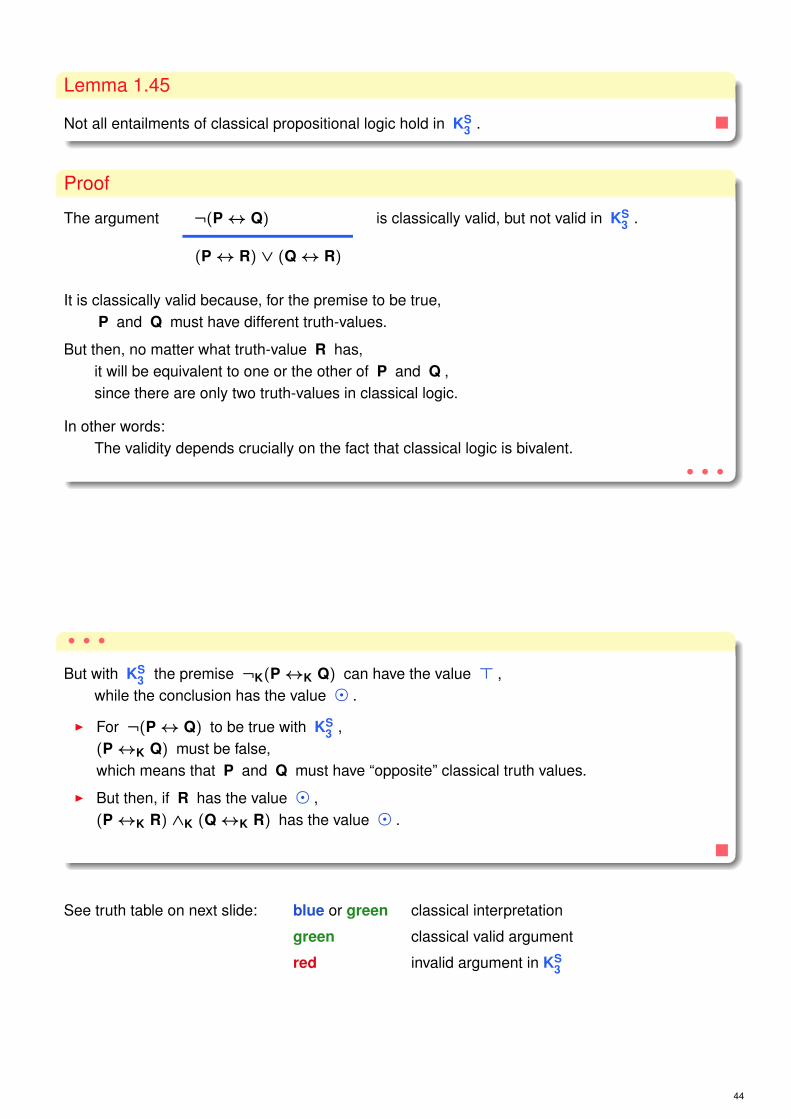
Lemma 1.45

Not all entailments of classical propositional logic hold in KS3 .

Proof

The argument ¬(P↔ Q)

(P↔ R) ∨ (Q↔ R)

is classically valid, but not valid in KS3 .

It is classically valid because, for the premise to be true,P and Q must have different truth-values.

But then, no matter what truth-value R has,it will be equivalent to one or the other of P and Q ,since there are only two truth-values in classical logic.

In other words:The validity depends crucially on the fact that classical logic is bivalent.

• • •

• • •

But with KS3 the premise ¬K(P↔K Q) can have the value > ,

while the conclusion has the value � .

I For ¬(P↔ Q) to be true with KS3 ,

(P↔K Q) must be false,which means that P and Q must have “opposite” classical truth values.

I But then, if R has the value � ,(P↔K R) ∧K (Q↔K R) has the value � .

See truth table on next slide: blue or green classical interpretation

green classical valid argument

red invalid argument in KS3

44

P Q R ¬K (P ↔K Q) ((P ↔K R) ∨K (Q ↔K R))

T T T ⊥ T T T T T T T T T TT T � ⊥ T T T T � � � T � �T T ⊥ ⊥ T T T T ⊥ ⊥ ⊥ T ⊥ ⊥T � T � T � � T T T T � � TT � � � T � � T � � � � � �T � ⊥ � T � � T ⊥ ⊥ � � � ⊥T ⊥ T T T ⊥ ⊥ T T T T ⊥ ⊥ TT ⊥ � T T ⊥ ⊥ T � � � ⊥ � �T ⊥ ⊥ T T ⊥ ⊥ T ⊥ ⊥ T ⊥ T ⊥� T T � � � T � � T T T T T� T � � � � T � � � � T � �� T ⊥ � � � T � � ⊥ � T ⊥ ⊥� � T � � � � � � T � � � T� � � � � � � � � � � � � �� ⊥ � � � � � � ⊥ � � � ⊥� ⊥ T � � � ⊥ � � T � ⊥ ⊥ T� ⊥ � � � � ⊥ � � � � ⊥ � �� ⊥ ⊥ � � � ⊥ � � ⊥ T ⊥ T ⊥⊥ T T T ⊥ ⊥ T ⊥ ⊥ T T T T T⊥ T � T ⊥ ⊥ T ⊥ � � � T � �⊥ T ⊥ T ⊥ ⊥ T ⊥ T ⊥ T T ⊥ ⊥⊥ � T � ⊥ � � ⊥ ⊥ T � � � T⊥ � � � ⊥ � � ⊥ � � � � � �⊥ � ⊥ � ⊥ � � ⊥ T ⊥ T � � ⊥⊥ ⊥ T ⊥ ⊥ T ⊥ ⊥ ⊥ T ⊥ ⊥ ⊥ T⊥ ⊥ � ⊥ ⊥ T ⊥ ⊥ � � � ⊥ � �⊥ ⊥ ⊥ ⊥ ⊥ T ⊥ ⊥ T ⊥ T ⊥ T ⊥

SEMANTICAL EQUIVALENCES

(P ∨K Q) ≡ (Q ∨K P) (P ∧K Q) ≡ (Q ∧K P)

(P ∨K (Q ∨K R)) ≡ ((P ∨K Q) ∨K R) (P ∧K (Q ∧K R)) ≡ ((P ∧K Q) ∧K R)

(P ∧K (Q ∨K R)) ≡ ((P ∧K Q) ∨K (P ∧K R))

(P ∨K (Q ∧K R)) ≡ ((P ∨K Q) ∧K (P ∨K R))

((P ∧K Q) ∨K P) ≡ P ((P ∨K Q) ∧K P) ≡ P

(P→K (Q→K R)) ≡ (Q→K (P→K R))

(P→K (Q→K R)) ≡ ((Q ∧K P)→K R)

Recall: There are no tautologies in KS3 !

46


ŁUKASIEWICZ

Jan Łukasiewicz21 December 1878 – 13 February 1956

I Poland contributed enormouslyto the development of Modern logic

I March 7, 1918: Talk at Warsaw University:First remarks about a 3-valued logic.

I A negation-implication version of a3-valued propositional logic[Łukasiewicz, 1920]

I Extended Article: [Łukasiewicz, 1930]

48

Manifold Motivations

I Future Contingents‘I shall be in Warsaw at noon

on December 21 of the next year’Being > or ⊥ at the moment of

utterance would cause determinism.=⇒� as possibility or indeterminacy?

I Doubts aboutthe Law of Non-Contradiction andthe Law of Excluded Middledue to suspected determinism

I ModalitiesTo formalize possibility and necessity

I First ideas about Logical probability– Counting valid instances of variables;– Counting models


Definition 1.46

An alphabet of Łukasiewicz’s 3-Valued Logic L3 consists of


I the set {¬ /1, ∧ /2, ∨ /2, →/2, ↔/2 } of (standard) connectives


Formulas of L3 are defined as with classical propositional logic.

Remark 1.47I Since 3-valued Łukasiewicz logic will be in the center of our attention,

we print its connectives in red instead of using an index.

I We will later consider a further unary connective T (Słupecki operator).

Remark 1.48We denote entailment in L3 by |= .

50

Definition 1.49

Truth Functions of L3

v ¬? v

T ⊥� �⊥ T

v ∧? w

v \ w T � ⊥

T T � ⊥� � � ⊥⊥ ⊥ ⊥ ⊥

v ∨? w

v \ w T � ⊥

T T T T

� T � �⊥ T � ⊥

v →? w

v \ w T � ⊥

T T � ⊥� T T �⊥ T T T

v ↔? w

v \ w T � ⊥

T T � ⊥� � T �⊥ ⊥ � T

NORMALITY, UNIFORMITY AND REGULARITY

Remark 1.50I Although the truth-tables for the connectives → and ↔ differ from Kleene’s truth-tables,

the L3 connectives are also both normal and uniform.

I Łukasiewicz’s truth-tables are NOT all regularThe truth-tables for the connectives → and ↔ are not regular,because of the middle rows or columns.

52

Example 1.51

P P ∨ ¬ P

T T T ⊥ T

� � � � �⊥ ⊥ T T ⊥

P Q P → (P → Q)

T T T T T T T

T � T � T � �T ⊥ T ⊥ T ⊥ ⊥� T � T � T T

� � � T � T �� ⊥ � T � � ⊥⊥ T ⊥ T ⊥ T T

⊥ � ⊥ T ⊥ T �⊥ ⊥ ⊥ T ⊥ T ⊥

P Q (P ∧ Q) → (P ∨ Q)

T T T T T T T T T

T � T � � T T T �T ⊥ T ⊥ ⊥ T T T ⊥� T � � T T � T T

� � � � � T � � �� ⊥ � ⊥ ⊥ T � � ⊥⊥ T ⊥ ⊥ T T ⊥ T T

⊥ � ⊥ ⊥ � T ⊥ � �⊥ ⊥ ⊥ ⊥ ⊥ T ⊥ ⊥ ⊥

Remark 1.52With L3 we may express F ≡ G in terms of connectives of L3 due to the following table.

F G (F ≡ G) ≡ ((F → G) ∧ (G → F))

T T T T T T T T T T T T TT � T ⊥ � ⊥ T � � � � T TT ⊥ T ⊥ ⊥ T T ⊥ ⊥ ⊥ ⊥ T T� T � ⊥ T ⊥ � T T � T � �� T � T � T � T � T �� ⊥ � ⊥ ⊥ ⊥ � � ⊥ � ⊥ T �⊥ T ⊥ ⊥ T T ⊥ T T ⊥ T ⊥ ⊥⊥ � ⊥ ⊥ � ⊥ ⊥ T � � � � ⊥⊥ ⊥ ⊥ T ⊥ T ⊥ T ⊥ T ⊥ T ⊥

This implies that for every interpretation of L3 holds:

FI = GI ⇐⇒ ((F→ G) ∧ (G→ F))I = >

⇐⇒ both (F→ G)I = > and (G→ F)I = > hold

Therefore, testing F ≡ G means testing both F→ G and G→ F resp. testing G↔ F .

This does not hold for KS3 !

54

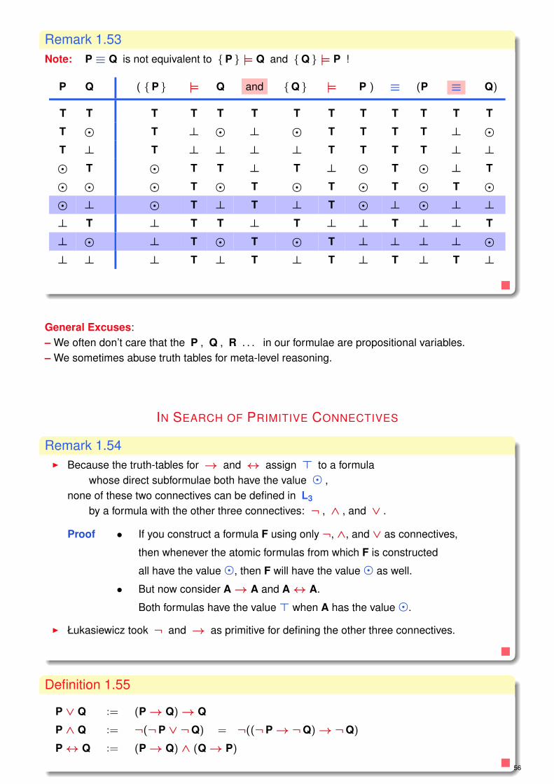
Remark 1.53Note: P ≡ Q is not equivalent to {P } |= Q and {Q } |= P !

P Q ( {P } |= Q and {Q } |= P ) ≡ (P ≡ Q)

T T T T T T T T T T T T T

T � T ⊥ � ⊥ � T T T T ⊥ �T ⊥ T ⊥ ⊥ ⊥ ⊥ T T T T ⊥ ⊥� T � T T ⊥ T ⊥ � T � ⊥ T

� � � T � T � T � T � T �� ⊥ � T ⊥ T ⊥ T � ⊥ � ⊥ ⊥⊥ T ⊥ T T ⊥ T ⊥ ⊥ T ⊥ ⊥ T

⊥ � ⊥ T � T � T ⊥ ⊥ ⊥ ⊥ �⊥ ⊥ ⊥ T ⊥ T ⊥ T ⊥ T ⊥ T ⊥

General Excuses:– We often don’t care that the P , Q , R . . . in our formulae are propositional variables.– We sometimes abuse truth tables for meta-level reasoning.

IN SEARCH OF PRIMITIVE CONNECTIVES

Remark 1.54I Because the truth-tables for → and ↔ assign > to a formula

whose direct subformulae both have the value � ,none of these two connectives can be defined in L3

by a formula with the other three connectives: ¬ , ∧ , and ∨ .

Proof • If you construct a formula F using only ¬, ∧, and ∨ as connectives,

then whenever the atomic formulas from which F is constructed

all have the value�, then F will have the value� as well.

• But now consider A→ A and A↔ A.

Both formulas have the value> when A has the value�.

I Łukasiewicz took ¬ and → as primitive for defining the other three connectives.

Definition 1.55

P ∨ Q := (P→ Q)→ Q

P ∧ Q := ¬(¬P ∨ ¬Q) = ¬((¬P→¬Q)→¬Q)

P↔ Q := (P→ Q) ∧ (Q→ P)

56

How to get the def of ∨ ? [Prior, 1953, p.320]

Prior compared the truth tables in L3 of formulae which are classically equivalent.

In L3 holds: P→ Q is not equivalent to ¬P ∨ Q , but a little weaker:P→ Q is implied by ¬P ∨ Q , but does not imply it.

P Q (¬ P ∨ Q) → (P → Q) (P → Q) → (¬ P ∨ Q)

T T ⊥ T T T T T T T T T T T ⊥ T T T

T � ⊥ T � � T T � � T � � T ⊥ T � �T ⊥ ⊥ T ⊥ ⊥ T T ⊥ ⊥ T ⊥ ⊥ T ⊥ T ⊥ ⊥� T � � T T T � T T � T T T � � T T

� � � � � � T � T � � T � � � � � �� ⊥ � � � ⊥ T � � ⊥ � � ⊥ T � � � ⊥⊥ T T ⊥ T T T ⊥ T T ⊥ T T T T ⊥ T T

⊥ � T ⊥ T � T ⊥ T � ⊥ T � T T ⊥ T �⊥ ⊥ T ⊥ T ⊥ T ⊥ T ⊥ ⊥ T ⊥ T T ⊥ T ⊥

The crucial case is the blue line.

Similarly, P ∨ Q is not equivalent to ¬P→ Q in L3 , but is a little stronger,¬P→ Q is implied by P ∨ Q , but does not imply it.

P Q (¬ P → Q) → (P ∨ Q) (P ∨ Q) → (¬ P → Q)

T T ⊥ T T T T T T T T T T T ⊥ T T T

T � ⊥ T T � T T T � T T � T ⊥ T T �T ⊥ ⊥ T T ⊥ T T T ⊥ T T ⊥ T ⊥ T T ⊥� T � � T T T � T T � T T T � � T T

� � � � T � � � � � � � � T � � T �� ⊥ � � � ⊥ T � � ⊥ � � ⊥ T � � � ⊥⊥ T T ⊥ T T T ⊥ T T ⊥ T T T T ⊥ T T

⊥ � T ⊥ � � T ⊥ � � ⊥ � � T T ⊥ � �⊥ ⊥ T ⊥ ⊥ ⊥ T ⊥ ⊥ ⊥ ⊥ ⊥ ⊥ T T ⊥ ⊥ ⊥

Again, the crucial case is the blue line.

Note the equivalence in the classical cases in both tables above.

58

Therefore, in order to define P ∨ Q in terms of → ,we require something which is a little stronger than ¬P→ Q in L3 ,but which in two-valued logic is equivalent to it;

for where the third truth-value is not involved,the tables in L3 for P ∨ Q and ¬P→ Q do coincide.

One procedure which in general increases the logical force of an implicative statement is theweakening of its antecedent.

I Thus, ’Bartholomew or Philip will come’being a weaker assertion than ’Philip will come’,

I ’If Bartholomew or Philip comes, I shall be surprised’is a stronger total assertion than ’If Philip comes I shall be surprised’.

However, there are cases in which this procedure will merely leave the force of the originalimplication unaltered.

For example, the statement

’If Bartholomew or Philip comes, Philip will come’

is not really any stronger an assertion than

’If Bartholomew comes Philip will come’,

since it will be true in any case that Philip will come if Philip comes.

A statement which is weaker than ¬P – the antecedent in our ¬P→ Q – is P→ Q :

For both in (classical) two-valued logic and in L3

’ ¬P ’ implies ’ P→ Q ’ whatever Q may be, but is not always implied by it.

Q P ¬ P → (P → Q)

T T ⊥ T T T T T

T � � � T � T T

T ⊥ T ⊥ T ⊥ T T

� T ⊥ T T T � �� T � T �� ⊥ T ⊥ T ⊥ T �⊥ T ⊥ T T T ⊥ ⊥⊥ � � � T � � ⊥⊥ ⊥ T ⊥ T ⊥ T ⊥

(P → Q) → ¬ P

T T T ⊥ ⊥ T

T � � � ⊥ T

T ⊥ ⊥ T ⊥ T

� T T � � �� T � � � �� ⊥ T � �⊥ T T T T ⊥⊥ T � T T ⊥⊥ T ⊥ T T ⊥

The green and blue rows shows that P→ Q is weaker than ¬P(The green rows are the classical cases.)

60

Hence the replacement of ¬P in ¬P→ Q by this weaker proposition P→ Q

will yield either a stronger assertion than the original ¬P→ Qor one equivalent to it;

and it turns out to yield an equivalent formula in (classical) two-valued logicand a stronger one in L3 .

In (classical) two-valued logic,

I the replacement of ¬P→ Q by (P→ Q)→ Qhas something of the artificiality of the replacement of

P→ Q by (P ∨ Q)→ Q in our example above,and makes no difference.

I In fact, it amounts to the replacement of ¬P→ Q by (¬P ∨ Q)→ Q ,since in classical logic P→ Q is equivalent to ¬P ∨ Q .

Note: (¬P ∨ Q)→ Q ≡ (P ∧ ¬Q) ∨ Q ≡ (P ∨ Q) ∧ (¬Q ∨ Q)

But in L3 , when P and Q have the truth-value �¬P→ Q and (P→ Q)→ Q will have different truth-values,the former being true and the latter not

and this is precisely the point at which in L3

the truth-tables for ¬P→ Q and P ∨ Q are different.

Q P ¬ P → Q (P → Q) → Q P ∨ Q

T T ⊥ T T T T T T T T T T T

T � � � T T T � � T � � T T

T ⊥ T ⊥ T T T ⊥ ⊥ T ⊥ ⊥ T T

� T ⊥ T T � � T T T T T T �� T � � T � � � � � �� ⊥ T ⊥ � � � � ⊥ � ⊥ ⊥ � �⊥ T ⊥ T T ⊥ ⊥ T T T T T T ⊥⊥ � � � � ⊥ ⊥ T � � � � � ⊥⊥ ⊥ T ⊥ ⊥ ⊥ ⊥ T ⊥ ⊥ ⊥ ⊥ ⊥ ⊥

Consequently, (P→ Q)→ Q serves ideally for the definition of P ∨ Q .

62

Lemma 1.56

I Every formula that is a tautology in L3 is also a tautology in classical logic, and

I every formula that is a contradiction in L3 is also a contradiction in classical logic.

ProofA formula F that is a tautology in L3

is also true in L3 on every classical truth-value assignment.

Since L3 is normal, it follows from the Normality Lemma 1.40that F is true on every interpretation in classical logic,and therefore, F is a tautology in classical logic.

Similar reasoning holds for contradictions.

Lemma 1.57

I Not every formula that is a tautology in classical logic is also a tautology in L3 , and

I not every formula that is a contradiction in classical logic is also a contradiction in L3 .

ProofI Any instance of the Law of the Excluded Middle, for example, A ∨ ¬A ,

is an example of a classical tautology that does not always have the value > in L3 .(see Example1.51)

I The formula A ∧ ¬A , which is a classical contradiction, is not a contradiction in L3 :It has the value � when A has the value � .

A A ∧ ¬ A

T T ⊥ ⊥ T

� � � � �⊥ ⊥ ⊥ T ⊥

• • •

64

• • •

Another example is the formula (P→ (Q→ R))→ ((P→ Q)→ (P→ R)) .This formula always has the value > in classical logic,

but in L3 it has the value �when P and Q have the value � and R has the value ⊥ . (see next slide)

Remark 1.58Note that Lemma 1.57 does not claim that all classical tautologies fail to be tautologies of L3

(nor that all classical contradictions fail to be contradictions of L3 ).

For example, A→ A is a tautology in both logics.

P Q R (P → (Q → R)) → ((P → Q) → (P → R))

T T T T T T T T T T T T T T T TT T � T � T � � T T T T � T � �T T ⊥ T ⊥ T ⊥ ⊥ T T T T ⊥ T ⊥ ⊥T � T T T � T T T T � � T T T TT � � T T � T � T T � � T T � �T � ⊥ T � � � ⊥ T T � � � T ⊥ ⊥T ⊥ T T T ⊥ T T T T ⊥ ⊥ T T T TT ⊥ � T T ⊥ T � T T ⊥ ⊥ T T � �T ⊥ ⊥ T T ⊥ T ⊥ T T ⊥ ⊥ T T ⊥ ⊥� T T � T T T T T � T T T � T T� T � � T T � � T � T T T � T �� T ⊥ � � T ⊥ ⊥ T � T T � � � ⊥� � T � T � T T T � T � T � T T� � � � T � T � T � T � T � T �� ⊥ � T � � ⊥ � � T � � � � ⊥� ⊥ T � T ⊥ T T T � � ⊥ T � T T� ⊥ � � T ⊥ T � T � � ⊥ T � T �� ⊥ ⊥ � T ⊥ T ⊥ T � � ⊥ T � � ⊥⊥ T T ⊥ T T T T T ⊥ T T T ⊥ T T⊥ T � ⊥ T T � � T ⊥ T T T ⊥ T �⊥ T ⊥ ⊥ T T ⊥ ⊥ T ⊥ T T T ⊥ T ⊥⊥ � T ⊥ T � T T T ⊥ T � T ⊥ T T⊥ � � ⊥ T � T � T ⊥ T � T ⊥ T �⊥ � ⊥ ⊥ T � � ⊥ T ⊥ T � T ⊥ T ⊥⊥ ⊥ T ⊥ T ⊥ T T T ⊥ T ⊥ T ⊥ T T⊥ ⊥ � ⊥ T ⊥ T � T ⊥ T ⊥ T ⊥ T �⊥ ⊥ ⊥ ⊥ T ⊥ T ⊥ T ⊥ T ⊥ T ⊥ T ⊥

66

Lemma 1.59

Not all entailments of classical propositional logic holds in L3 .

ProofThe argument in Lemma 1.45 will suffice here as well:

The argument ¬(P↔ Q)

(P↔ R) ∨ (Q↔ R)

is classically valid, but not valid in L3 .

Recall: If ¬(P↔ Q) is true, then P and Q must have different truth-values.But then R ’s truth-value will be equivalent to one or the other of P and Q .

As with KS3 , with L3 the premise ¬(P↔ Q) can only have the value > ,

if P and Q have “opposite” classical truth values.However, if R has the value � , then the conclusion has the truth value � .



red invalid argument in L3 and

differences to KS3 in the truth table

P Q R ¬ (P ↔ Q) ≡ ((P ↔ R) ∨ (Q ↔ R))

T T T ⊥ T T T ⊥ T T T T T T TT T � ⊥ T T T ⊥ T � � � T � �T T ⊥ ⊥ T T T T T ⊥ ⊥ ⊥ T ⊥ ⊥T � T � T � � ⊥ T T T T � � TT � � � T � � ⊥ T � � T � T �T � ⊥ � T � � T T ⊥ ⊥ � � � ⊥T ⊥ T T T ⊥ ⊥ T T T T T ⊥ ⊥ TT ⊥ � T T ⊥ ⊥ ⊥ T � � � ⊥ � �T ⊥ ⊥ T T ⊥ ⊥ T T ⊥ ⊥ T ⊥ T ⊥� T T � � � T ⊥ � � T T T T T� T � � � � T ⊥ � T � T T � �� T ⊥ � � � T T � � ⊥ � T ⊥ ⊥� � T ⊥ � T � ⊥ � � T � � � T� � � ⊥ � T � ⊥ � T � T � T �� ⊥ ⊥ � T � ⊥ � � ⊥ � � � ⊥� ⊥ T � � � ⊥ T � � T � ⊥ ⊥ T� ⊥ � � � � ⊥ ⊥ � T � T ⊥ � �� ⊥ ⊥ � � � ⊥ ⊥ � � ⊥ T ⊥ T ⊥⊥ T T T ⊥ ⊥ T T ⊥ ⊥ T T T T T⊥ T � T ⊥ ⊥ T ⊥ ⊥ � � � T � �⊥ T ⊥ T ⊥ ⊥ T T ⊥ T ⊥ T T ⊥ ⊥⊥ � T � ⊥ � � T ⊥ ⊥ T � � � T⊥ � � � ⊥ � � ⊥ ⊥ � � T � T �⊥ � ⊥ � ⊥ � � ⊥ ⊥ T ⊥ T � � ⊥⊥ ⊥ T ⊥ ⊥ T ⊥ T ⊥ ⊥ T ⊥ ⊥ ⊥ T⊥ ⊥ � ⊥ ⊥ T ⊥ ⊥ ⊥ � � � ⊥ � �⊥ ⊥ ⊥ ⊥ ⊥ T ⊥ ⊥ ⊥ T ⊥ T ⊥ T ⊥

68

Remark 1.60We note that other classically valid arguments are valid in L3 .

For example, the classically valid argument P

P→ Q

Q

is valid in L3 (as well as in KS3 ).

TODO: table

P Q P P → Q Q

T T T T T T T

T � T T � � �T ⊥ T T ⊥ ⊥ ⊥� T � � T T T

� � � � T � �� ⊥ � � � ⊥ ⊥⊥ T ⊥ ⊥ T T T

⊥ � ⊥ ⊥ T � �⊥ ⊥ ⊥ ⊥ T ⊥ ⊥

TODO: parbox



The red T is thedifference between→ and →K


BOCHVAR

Dmitri Bochvar (1909 – 1994)

I Liar Paradox‘This sentence is false.’

I Russel’s antinomy

I Bochvar’s ConclusionsThis sentence is meaningless

and hence neither true nor false,since only meaningful sentences

can say true or false things.

=⇒� represents meaninglessness

I Resulting SystemCombination of two sets of connectives:

– internal system BI3

(= Kleene’s weak logic)

– external system BE3

I [Bochvar, 1937]


Definition 1.61

An alphabet of Bochvar’s internal 3-valued Logic BI3 consists of


I the set {¬BI/1, ∧BI/2, ∨BI/2, →BI/2, ↔BI/2 } of (standard) connectives


Formulas of BI3 are defined as with classical propositional logic.

72

Definition 1.62

Truth Functions of BI3

v ¬?BI v

T ⊥� �⊥ T

v ∧?BI w

v \ w T � ⊥

T T � ⊥� � � �⊥ ⊥ � ⊥

v ∨?BI w

v \ w T � ⊥

T T � T

� � � �⊥ T � ⊥

v →?BI w

v \ w T � ⊥

T T � ⊥� � � �⊥ T � T

v ↔?BI w

v \ w T � ⊥

T T � ⊥� � � �⊥ ⊥ � T

CONTAGIOUS TRUTH VALUES

Definition 1.63The truth-value � is contagious in BI

3 :

Whenever a component of a compound formula has the value � ,so does the compound formula as a whole, regardless of the value of any other component.

Remark 1.64If the truth value � represents meaninglessness (or absence of meaning),then it is quite reasonable that this truth value should be contagious.

74

KLEENE’S WEAK 3-VALUED LOGIC

Remark 1.65Kleene also defined a second system of 3-valued connectives,

which he called the weak connectives.

That system is identical to BI3 .

We shall nevertheless refer to this system as Bochvar’s.

Kleene was motivated by non-terminating computations.


Remark 1.66

I All connectives of BI3 are normal.

I All connectives of BI3 are regular, but not the strongest regular ones.

I Of the binary connectives only the biconditional is uniform.

. Uniformity of conjunction, for example,would require that a conjunction to be false whenever one of the conjuncts is.But since the value � is contagious, this is not the case.Consequently, conjunction is not uniform.

. Similarly, neither disjunction nor the conditional are uniform in BI3

76

INTERDEFINABILITY

Remark 1.67As with KS

3 , any way of interdefining connectives in classical logic will also works for BI3 .

This is because not only are the connectives normal,but they all agree on what happens when a formula has a component with the value �(namely, the compound formula is also assigned the value � ).

Bochvar chose ¬BI and ∧BI as primitive connectives and defined:

F ∨BI G := ¬BI(¬BI F ∧BI ¬BI G)

F→BI G := ¬BI(F ∧BI ¬BI G)

F↔BI G := (F→BI G) ∧BI (G→BI F)

Example 1.68

P P ∨BI ¬BI P

T T T ⊥ T

� � � � �⊥ ⊥ T T ⊥

P Q P →BI (P →BI Q)

T T T T T T T

T � T � T � �T ⊥ T ⊥ T ⊥ ⊥� T � � � � T

� � � � � � �� ⊥ � � � � ⊥⊥ T ⊥ T ⊥ T T

⊥ � ⊥ � ⊥ � �⊥ ⊥ ⊥ T ⊥ T ⊥

P Q (P ∧BI Q) →BI (P ∨BI Q)

T T T T T T T T T

T � T � � � T � �T ⊥ T ⊥ ⊥ T T T ⊥� T � � T � � � T

� � � � � � � � �� ⊥ � � ⊥ � � � ⊥⊥ T ⊥ ⊥ T T ⊥ T T

⊥ � ⊥ � � � ⊥ � �⊥ ⊥ ⊥ ⊥ ⊥ T ⊥ ⊥ ⊥

– Neither of the classical tautologies is a tautology in BI3 .

– The second formula receives the value � more often in BI3 than it did in KS

3 or L3 .

78

Lemma 1.69

No formula is a tautology in BI3 , and no formula is a contradiction in BI

3 .

Remark 1.70Because � is contagious,every formula has the value � on at least one truth-value assignment to its atomic components,namely, on any truth-value assignment that assigns � to at least one atomic component.Therefore, no formula is true under every interpretation of BI

3 .

Analogously, there are no contradictions.

Lemma 1.71

For every formula F in BI3 holds: If S |= BI F then S |= F .

ProofThis follows from the Normality Lemma 1.40 since BI

3 is normal.

Lemma 1.72

Not every entailment that holds in classical propositional logic holds in BI3 as well.

Proof

The example argument ¬(P↔ Q)

(P↔ R) ∨ (Q↔ R)

and truth-value assignment in Lemma 1.45 suffice here as well. Note: ↔?BI = ↔?

K



red invalid argument in BI3 and

differences to KS3 in the truth table

(just in the ∨BI column)

Note: We are comparing Kleene’s strong with Kleene’s weak 3-valued logic!

80

P Q R ¬BI (P ↔BI Q) ((P ↔BI R) ∨BI (Q ↔BI R))

T T T ⊥ T T T T T T T T T TT T � ⊥ T T T T � � � T � �T T ⊥ ⊥ T T T T ⊥ ⊥ ⊥ T ⊥ ⊥T � T � T � � T T T � � � TT � � � T � � T � � � � � �T � ⊥ � T � � T ⊥ ⊥ � � � ⊥T ⊥ T T T ⊥ ⊥ T T T T ⊥ ⊥ TT ⊥ � T T ⊥ ⊥ T � � � ⊥ � �T ⊥ ⊥ T T ⊥ ⊥ T ⊥ ⊥ T ⊥ T ⊥� T T � � � T � � T � T T T� T � � � � T � � � � T � �� T ⊥ � � � T � � ⊥ � T ⊥ ⊥� � T � � � � � � T � � � T� � � � � � � � � � � � � �� ⊥ � � � � � � ⊥ � � � ⊥� ⊥ T � � � ⊥ � � T � ⊥ ⊥ T� ⊥ � � � � ⊥ � � � � ⊥ � �� ⊥ ⊥ � � � ⊥ � � ⊥ � ⊥ T ⊥⊥ T T T ⊥ ⊥ T ⊥ ⊥ T T T T T⊥ T � T ⊥ ⊥ T ⊥ � � � T � �⊥ T ⊥ T ⊥ ⊥ T ⊥ T ⊥ T T ⊥ ⊥⊥ � T � ⊥ � � ⊥ ⊥ T � � � T⊥ � � � ⊥ � � ⊥ � � � � � �⊥ � ⊥ � ⊥ � � ⊥ T ⊥ � � � ⊥⊥ ⊥ T ⊥ ⊥ T ⊥ ⊥ ⊥ T ⊥ ⊥ ⊥ T⊥ ⊥ � ⊥ ⊥ T ⊥ ⊥ � � � ⊥ � �⊥ ⊥ ⊥ ⊥ ⊥ T ⊥ ⊥ T ⊥ T ⊥ T ⊥

Remark 1.73

The argument Q

P→ Q

which is valid in both KS3 and L3 (due to uniformity),

is not valid in BI3 .

Assuming the premise Q to have the value > .

Then, the conclusion has the value � in BI3 ,

if Q has the value > and P has the value � .

P Q Q P →BI Q

T T T T T T

T � � T � �T ⊥ ⊥ T ⊥ ⊥� T T � � T

� � � � � �� ⊥ ⊥ � � ⊥⊥ T T ⊥ T T

⊥ � � ⊥ � �⊥ ⊥ ⊥ ⊥ T ⊥



red:invalid argument in BI

3

82

Remark 1.74

The classically valid argument P

P→ Q

Q

is also valid in BI3 .

P Q P P →BI Q Q

T T T T T T T

T � T T � � �T ⊥ T T ⊥ ⊥ ⊥� T � � � T T

� � � � � � �� ⊥ � � � ⊥ ⊥⊥ T ⊥ ⊥ T T T

⊥ � ⊥ ⊥ � � �⊥ ⊥ ⊥ ⊥ T ⊥ ⊥





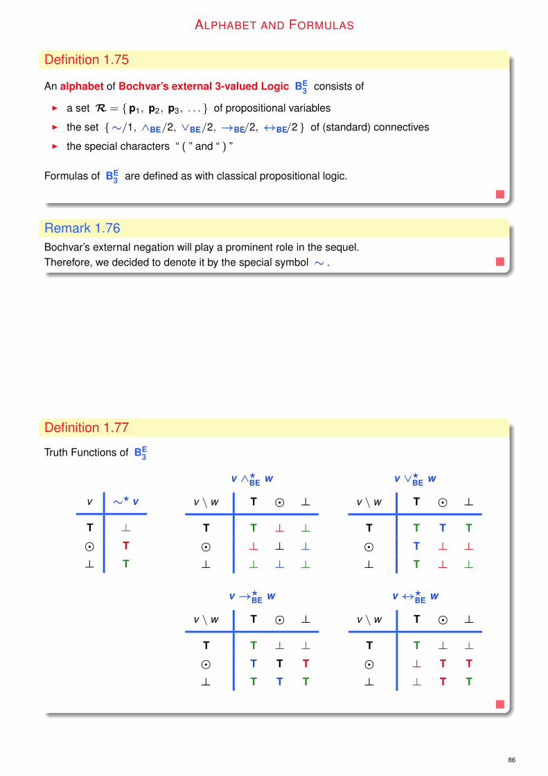
Definition 1.75

An alphabet of Bochvar’s external 3-valued Logic BE3 consists of


I the set {∼/1, ∧BE/2, ∨BE/2, →BE/2, ↔BE/2 } of (standard) connectives


Formulas of BE3 are defined as with classical propositional logic.

Remark 1.76Bochvar’s external negation will play a prominent role in the sequel.Therefore, we decided to denote it by the special symbol ∼ .

Definition 1.77

Truth Functions of BE3

v ∼? v

T ⊥� T

⊥ T

v ∧?BE w

v \ w T � ⊥

T T ⊥ ⊥� ⊥ ⊥ ⊥⊥ ⊥ ⊥ ⊥

v ∨?BE w

v \ w T � ⊥

T T T T

� T ⊥ ⊥⊥ T ⊥ ⊥

v →?BE w

v \ w T � ⊥

T T ⊥ ⊥� T T T

⊥ T T T

v ↔?BE w

v \ w T � ⊥

T T ⊥ ⊥� ⊥ T T

⊥ ⊥ T T

86


Remark 1.78I All standard connectives of BE

3 are normal.

I None of the standard connectives of BE3 is regular.

(obvious infractions are marked as red in tables above)

I All standard connectives of BE3 are uniform (blue entries).

Remark 1.79

All the connectives in BE3 treat the truth value � as if it were ⊥ .

Remark 1.80Good suggestive readings of ∼F are:

I F is not true

I F is true doesn’t hold

Example 1.81

P P ∨BE ∼ P

T T T ⊥ T

� � T T �⊥ ⊥ T T ⊥

P Q P →BE (P →BE Q)

T T T T T T T

T � T ⊥ T ⊥ �T ⊥ T ⊥ T ⊥ ⊥� T � T � T T

� � � T � T �� ⊥ � T � T ⊥⊥ T ⊥ T ⊥ T T

⊥ � ⊥ T ⊥ T �⊥ ⊥ ⊥ T ⊥ T ⊥

P Q (P ∧BE Q)→BE (P ∨BE Q)

T T T T T T T T T

T � T ⊥ � T T T �T ⊥ T ⊥ ⊥ T T T ⊥� T � ⊥ T T � T T

� � � ⊥ � T � ⊥ �� ⊥ � ⊥ ⊥ T � ⊥ ⊥⊥ T ⊥ ⊥ T T ⊥ T T

⊥ � ⊥ ⊥ � T ⊥ ⊥ �⊥ ⊥ ⊥ ⊥ ⊥ T ⊥ ⊥ ⊥

The classical tautologies P ∨ ¬P and (P ∧ Q)→ (P ∨ Q) remain tautologies in BE3 .

88

Lemma 1.82

The set of tautologies in BE3 is exactly the set of tautologies in classical logic,

and the set of contradictions in BE3 is exactly the set of contradictions in classical logic.

Proof=⇒ Since BE

3 is normal, it follows from the Normality Lemma 1.40that every formula that is a tautology in BE

3 is a classical tautology,and similarly for contradictions.

⇐= Conversely, assume F to be a classical tautology. Then F is a compound formula.

Since the connectives in BE3 treat their � components as if they were ⊥ ,

BE3 treats the atomic components of any compound formula

on an interpretation where they are � as if they were ⊥ . (cf. Remark 1.79)

Consequently,BE

3 assigns the same truth-value to the formula that classical logic would in that case.Therefore, F must be a tautology in BE

3 as well.

Similar reasoning holds for contradictions.

Lemma 1.83

For every formula F in BE3 holds: If S |= BE F then S |= F .

ProofThis follows from the Normality Lemma 1.40, since BE

3 is normal.

Lemma 1.84

For every formula F in BE3 holds: If S |= F then S |= BE F .

90

ProofWe shall show this by contraposition: We’ll show that

if an entailment does not hold in BE3 ,

then it doesn’t hold in classical logic either.

So consider a set S and formula F such that S |/= BE F .

Then there is some 3-valued assignment I on which all the formulas in Shave the value > , but on which F has either the value ⊥ or the value � .

We can convert I to a classical truth-value assignment Jby keeping the > and ⊥ assignments to atomic formulas,but turning the � assignments (if any) to atomic formulas into ⊥ assignments.

This classical truth-value assignment J will make formulas in S true in classical logic,

I because compound formulas in Sbehave in BE

3 as if their � -valued atomic components have the value ⊥ ,

I and if any of the formulas in S are atomic, then,since they have the value > on the original BE

3 assignment I ,they will have the value > on the classical assignment J as well.

But F has the value ⊥ on the classical truth-value assignment J for similar reasons.

Classical valid argument (which had failed for KS3 , L3 and BI

3 ): ( CL : green, BE3 : blue)

P Q R ∼ (P ↔BE Q) ≡ ((P ↔BE R) ∨BE (Q ↔BE R))

T T T ⊥ T T T ⊥ T T T T T T TT T � ⊥ T T T T T ⊥ � ⊥ T ⊥ �T T ⊥ ⊥ T T T T T ⊥ ⊥ ⊥ T ⊥ ⊥T � T T T ⊥ � T T T T T � ⊥ TT � � T T ⊥ � T T ⊥ � T � T �T � ⊥ T T ⊥ � T T ⊥ ⊥ T � T ⊥T ⊥ T T T ⊥ ⊥ T T T T T ⊥ ⊥ TT ⊥ � T T ⊥ ⊥ T T ⊥ � T ⊥ T �T ⊥ ⊥ T T ⊥ ⊥ T T ⊥ ⊥ T ⊥ T ⊥� T T T � ⊥ T T � ⊥ T T T T T� T � T � ⊥ T T � T � T T ⊥ �� T ⊥ T � ⊥ T T � T ⊥ T T ⊥ ⊥� � T ⊥ � T � T � ⊥ T ⊥ � ⊥ T� � � ⊥ � T � ⊥ � T � T � T �� ⊥ ⊥ � T � ⊥ � T ⊥ T � T ⊥� ⊥ T ⊥ � T ⊥ T � ⊥ T ⊥ ⊥ ⊥ T� ⊥ � ⊥ � T ⊥ ⊥ � T � T ⊥ T �� ⊥ ⊥ ⊥ � T ⊥ ⊥ � T ⊥ T ⊥ T ⊥⊥ T T T ⊥ ⊥ T T ⊥ ⊥ T T T T T⊥ T � T ⊥ ⊥ T T ⊥ T � T T ⊥ �⊥ T ⊥ T ⊥ ⊥ T T ⊥ T ⊥ T T ⊥ ⊥⊥ � T ⊥ ⊥ T � T ⊥ ⊥ T ⊥ � ⊥ T⊥ � � ⊥ ⊥ T � ⊥ ⊥ T � T � T �⊥ � ⊥ ⊥ ⊥ T � ⊥ ⊥ T ⊥ T � T ⊥⊥ ⊥ T ⊥ ⊥ T ⊥ T ⊥ ⊥ T ⊥ ⊥ ⊥ T⊥ ⊥ � ⊥ ⊥ T ⊥ ⊥ ⊥ T � T ⊥ T �⊥ ⊥ ⊥ ⊥ ⊥ T ⊥ ⊥ ⊥ T ⊥ T ⊥ T ⊥

92

BOCHVAR’S ASSERTION OPERATOR

Definition 1.85Bochvar introduced both the internal and external connectives within a single system.

In that system the external connectives were defined connectives,

using the internal connectives and a special external assertion operator,

the connective a . v a? v

T T

� ⊥⊥ ⊥

Intuitive meaning of a P : P is true

P a P

T T P is true holds

� ⊥ P is true doesn’t hold

⊥ ⊥ P is true doesn’t hold

Lemma 1.86The external version ◦BE of a n-ary connective ◦ may be defined

by applying the respective internal version ◦BI of the connectiveto externally asserted formulas:

◦BE(F1, . . . ,Fn) := ◦BI(a F1, . . . , a Fn)

Thus, both the internal and the external connectives can be defined in terms of ¬BI , ∧BI and a.

Thus, for example, if we apply the internal ¬BI to a P , we get the table for external negation:

P ¬BI a P ≡ ∼P

T ⊥ T T ⊥� T ⊥ T T

⊥ T ⊥ T T

94

If we apply the binary internal connectives to a P and a Q ,we get the table for the respective binary external connectives.

P Q (a P ∧BI a Q) ≡ (P ∧BE Q)

T T T T T T T T T T T

T � T T ⊥ ⊥ � T T ⊥ �T ⊥ T T ⊥ ⊥ ⊥ T T ⊥ ⊥� T ⊥ � ⊥ T T T � ⊥ T

� � ⊥ � ⊥ ⊥ � T � ⊥ �� ⊥ ⊥ � ⊥ ⊥ ⊥ T � ⊥ ⊥⊥ T ⊥ ⊥ ⊥ T T T ⊥ ⊥ T

⊥ � ⊥ ⊥ ⊥ ⊥ � T ⊥ ⊥ �⊥ ⊥ ⊥ ⊥ ⊥ ⊥ ⊥ T ⊥ ⊥ ⊥

P Q (a P ∨BI a Q) ≡ (P ∨BE Q)


T � T T T ⊥ � T T T �T ⊥ T T T ⊥ ⊥ T T T ⊥� T ⊥ � T T T T � T T

� � ⊥ � ⊥ ⊥ � T � ⊥ �� ⊥ ⊥ � ⊥ ⊥ ⊥ T � ⊥ ⊥⊥ T ⊥ ⊥ T T T T ⊥ T T

⊥ � ⊥ ⊥ ⊥ ⊥ � T ⊥ ⊥ �⊥ ⊥ ⊥ ⊥ ⊥ ⊥ ⊥ T ⊥ ⊥ ⊥

P Q (a P →BI a Q) ≡ (P →BE Q)


T � T T ⊥ ⊥ � T T ⊥ �T ⊥ T T ⊥ ⊥ ⊥ T T ⊥ ⊥� T ⊥ � T T T T � T T

� � ⊥ � T ⊥ � T � T �� ⊥ ⊥ � T ⊥ ⊥ T � T ⊥⊥ T ⊥ ⊥ T T T T ⊥ T T

⊥ � ⊥ ⊥ T ⊥ � T ⊥ T �⊥ ⊥ ⊥ ⊥ T ⊥ ⊥ T ⊥ T ⊥

P Q (a P ↔BI a Q) ≡ (P ↔BE Q)


T � T T ⊥ ⊥ � T T ⊥ �T ⊥ T T ⊥ ⊥ ⊥ T T ⊥ ⊥� T ⊥ � ⊥ T T T � ⊥ T

� � ⊥ � T ⊥ � T � T �� ⊥ ⊥ � T ⊥ ⊥ T � T ⊥⊥ T ⊥ ⊥ ⊥ T T T ⊥ ⊥ T

⊥ � ⊥ ⊥ T ⊥ � T ⊥ T �⊥ ⊥ ⊥ ⊥ T ⊥ ⊥ T ⊥ T ⊥

96

Definition 1.87The external assertion operator can be defined as follows: a P := ∼∼P

P a P ≡ ∼ ∼ P a P ≡ ¬ ∼ P

T T T T ⊥ T T T T ⊥ T

� ⊥ T ⊥ T � ⊥ T ⊥ T �⊥ ⊥ T ⊥ T ⊥ ⊥ T ⊥ T ⊥

Remark 1.88

Note that ∼ is not involutive! P P ≡ ∼ ∼ P

T T T T ⊥ T

� � ⊥ ⊥ T �⊥ ⊥ T ⊥ T ⊥

2. Definability of ConnectivesInterdefinability of ConnectivesDefining Normal Connectives with Łukasiewicz 3-valued LogicDefining Non-Normal ConnectivesŁukasiewicz’s Bold Connectives


DEFINABILITY & COMPLETE SET OF CONNECTIVES

Definition 2.1

For an arbitrary propositional logic L with R = {p1, p2, p3, . . . } we define:

I An n-ary connective ◦ is definable by a set C = {◦1, . . . ,◦k } of connectives ⇐⇒there exists a formula F in which occur

. at most connectives from C and

. at most the propositional variables p1 to pn

and such that ◦ (p1, . . . ,pn) ≡ F holds.

I A set C = {◦1, . . . ,◦k } of connectives is complete ⇐⇒if every connective is definable by C .

Remark 2.2A many-valued logic is basically given by its set of connectives

– usually the standard connectives, maybe some additional ones.

We say that a connective ◦ is definable in a logic L ⇐⇒◦ is definable by the set of connectives of L.

100

Lemma 2.3

The binary connectives of KS3 , L3 , and BE

3 are not definable in BI3 .

ProofNone of the connectives in BI

3 produces a formula with a classical truth-valuewhen any of its immediate components have the value � (due to contagiousness).

But the binary connectives of the other three systems can produce such formulae,so none of these connectives can be defined using only the connectives of BI

3 .

Lemma 2.4

None of the connectives of KS3 , L3 , or BI

3 are definable in BE3 .

ProofThe connectives of BE

3 never produce formulas with the value � .Since each of the connectives in the other systems can produce such formulas,the result follows.

Lemma 2.5

All of the connectives of BI3 are definable in both KS

3 and L3 .

ProofI Negation in BI

3 is identical to negation in the other two systems.

I We can define BI3 ’s conjunction ∧BI using conjunction, disjunction, and negation of L3

(which are identical to those in KS3 ) as follows:

P ∧BI Q := (P ∧ Q) ∨ ((P ∧ ¬P) ∨ (Q ∧ ¬Q))

I We can then define the other BI3 connectives in terms of these two,

using any of the standard classical equivalences.

Alternatively, we can give direct definitions for ∨BI and →BI

analogous to the preceding definition for ∧BI :

P ∨BI Q := (P ∨ Q) ∧ ((P ∨ ¬P) ∧ (Q ∨ ¬Q))

P→BI Q := (¬P ∨ Q) ∧ ((P ∨ ¬P) ∧ (Q ∨ ¬Q))

(See the next slides for a verification by truth tables.)

102

P Q (P ∧BI Q) ≡ ((P ∧ Q) ∨ ((P ∧ ¬ P) ∨ (Q ∧ ¬ Q )))

T T T T T T T T T T T ⊥ ⊥ T ⊥ T ⊥ ⊥ T

T � T � � T T � � � T ⊥ ⊥ T � � � � �T ⊥ T ⊥ ⊥ T T ⊥ ⊥ ⊥ T ⊥ ⊥ T ⊥ ⊥ ⊥ T ⊥� T � � T T � � T � � � � � � T ⊥ ⊥ T

� � � � � T � � � � � � � � � � � � �� ⊥ � � ⊥ T � ⊥ ⊥ � � � � � � ⊥ ⊥ T ⊥⊥ T ⊥ ⊥ T T ⊥ ⊥ T ⊥ ⊥ ⊥ T ⊥ ⊥ T ⊥ ⊥ T

⊥ � ⊥ � � T ⊥ ⊥ � � ⊥ ⊥ T ⊥ � � � � �⊥ ⊥ ⊥ ⊥ ⊥ T ⊥ ⊥ ⊥ ⊥ ⊥ ⊥ T ⊥ ⊥ ⊥ ⊥ T ⊥

P Q (P ∨BI Q) ≡ ((P ∨ Q) ∧ ((P ∨ ¬ P) ∧ (Q ∨ ¬ Q )))

T T T T T T T T T T T T ⊥ T T T T ⊥ TT � T � � T T T � � T T ⊥ T � � � � �T ⊥ T T ⊥ T T T ⊥ T T T ⊥ T T ⊥ T T ⊥� T � � T T � T T � � � � � � T T ⊥ T� � � � � T � � � � � � � � � � � � �� ⊥ � � ⊥ T � � ⊥ � � � � � � ⊥ T T ⊥⊥ T ⊥ T T T ⊥ T T T ⊥ T T ⊥ T T T ⊥ T⊥ � ⊥ � � T ⊥ � � � ⊥ T T ⊥ � � � � �⊥ ⊥ ⊥ ⊥ ⊥ T ⊥ ⊥ ⊥ ⊥ ⊥ T T ⊥ T ⊥ T T ⊥

P Q (P →BI Q) ≡ ((¬ P ∨ Q) ∧ ((P ∨ ¬ P) ∧ (Q ∨ ¬ Q )))

T T T T T T ⊥ T T T T T T ⊥ T T T T ⊥ TT � T � � T ⊥ T � � � T T ⊥ T � � � � �T ⊥ T ⊥ ⊥ T ⊥ T ⊥ ⊥ ⊥ T T ⊥ T T ⊥ T T ⊥� T � � T T � � T T � � � � � � T T ⊥ T� � � � � T � � � � � � � � � � � � � �� ⊥ � � ⊥ T � � � ⊥ � � � � � � ⊥ T T ⊥⊥ T ⊥ T T T T ⊥ T T T ⊥ T T ⊥ T T T ⊥ T⊥ � ⊥ � � T T ⊥ T � � ⊥ T T ⊥ � � � � �⊥ ⊥ ⊥ T ⊥ T T ⊥ T ⊥ T ⊥ T T ⊥ T ⊥ T T ⊥

104

Lemma 2.6

The L3 conditional → is not definable in KS3 .

ProofA formula P→ Q has the value > when both P and Q have the value � .But every KS

3 connective produces a formula with the value �when its immediate components (all) have the value � ,so no combination of KS

3 connectives can produce a formula that expresses the L3 conditional.

Lemma 2.7

The BE3 connectives are not definable in KS

3 .

ProofNo KS

3 connective produces a formula that has a classical truth-valuewhen its immediate components have the value � ,so no BE

3 connective can be defined using KS3 connectives.

Lemma 2.8

Every KS3 connective is definable in L3 .

ProofI Negation, conjunction, and disjunction of KS

3 are identical to those of L3 .

I The conditional and biconditional of KS3 are definable using those connectives.

106

Lemma 2.9

Every BE3 connective is definable in L3 .

ProofIt will suffice to show that Bochvar’s external assertion is definable in L3 .

The equivalence a P ≡ ¬(P→¬P) (≡ ¬(P→¬P))

produces the table for external assertion:

P a P ¬ (P → ¬ P)

T T T T ⊥ ⊥ T

� ⊥ ⊥ � T � �⊥ ⊥ ⊥ ⊥ T T ⊥

Now, all BE3 connectives are definable in L3 , since

I all of the other external Bochvar connectives can be defined using external assertion aand Bochvar’s internal connectives,

I Bochvar’s internal connectives are definable in L3 (Lemma 2.5).

OVERVIEW: NON ŁUKASIEWICZ CONNECTIVES

¬K P ≡ ¬P (identical truth function)

∧K P ≡ ∧ P (identical truth function)

∨K P ≡ ∨ P (identical truth function)

P→K Q ≡ ¬P ∨ Q (≡ ¬K P ∨K Q )

P↔K Q ≡ (¬P ∨ Q) ∧ (¬Q ∨ P) (≡ (P→K Q) ∧K (Q→K P) )

a P ≡ ¬(P→¬P)

¬BI P ≡ ¬P (identical truth function)

P ∨BI Q ≡ (P ∨ Q) ∧ ((P ∨ ¬P) ∧ (Q ∨ ¬Q))

P ∧BI Q ≡ (P ∧ Q) ∨ ((P ∧ ¬P) ∨ (Q ∧ ¬Q)) (≡ ¬BI(¬BI P ∧BI ¬BI Q) )

P→BI Q ≡ (¬P ∨ Q) ∧ ((P ∨ ¬P) ∧ (Q ∨ ¬Q)) (≡ ¬BI(P ∧BI ¬BI Q) )

P↔BI Q ≡ (P→BI Q) ∧ (Q→BI P) ≡ · · · (≡ P↔K Q )

∼P ≡ ¬ a P ≡ ¬¬(P→¬P) ≡ (P→¬P)

P ∨BE Q ≡ a P ∨BI a Q ≡ ¬(P→¬P) ∨ ¬(Q→¬Q)

P ∧BE Q ≡ a P ∧BI a Q ≡ ¬(P→¬P) ∧ ¬(Q→¬Q)

P→BE Q ≡ a P→BI a Q ≡ ∼P ∨ a Q ≡ (P→¬P) ∨ ¬(Q→¬Q)

P↔BE Q ≡ a P↔BI a Q ≡ · · ·

108


COMPLETE SETS OF CONNECTIVES

Remark 2.10I We have shown that L3 is powerful enough to define all connectives of KS

3 , BI3 and BE

3 .

Question Are all possible 3-valued connectives definable in L3 ?

If they are, then the (standard/primitive) connectives of L3 are a complete set of connectives.

I Recall: For classical logic exist complete sets of connectives,e.g., {→,¬ } , {∨,¬ } , . . .

Example 2.11Is the connective # with the truth function #? definable in L3 ?

v#?w : v \ w T � ⊥

T T � T

� T � �⊥ ⊥ � ⊥

110

CLASSICAL CASE

Which formula defines the classical connective # obtained by restriction to W2 ?

P Q P # Q

T T T

T ⊥ T

⊥ T ⊥⊥ ⊥ ⊥

Answer: (P ∧ Q) ∨ (P ∧ ¬Q)

Procedure: We build a suitable full conjunction for every row which results in > .These full conjunctions are then combined disjunctively.

Remark: This procedure doesn’t always produce the simplest definition!

DEFINABILITY OF NORMAL CONNECTIVES

Lemma 2.12All normal 3-valued truth-functions are definable in L3 .

ProofA normal 3-valued n -ary truth-function f can be described by the truth-tablefor a formula with a corresponding n -ary connective @ , i.e. @? = f .

P1 P2 . . . Pn @(P1, . . . ,Pn)

T T . . . T v1

T T . . . � v2...

...

⊥ ⊥ . . . ⊥ v3n

I where each of v1 , v2 , . . . , v3n is one of the values > , � , ⊥ and

I where vi is > or ⊥if all of the values to the left of the vertical bar in row i are classical truth-values.

• • •

112

• • •

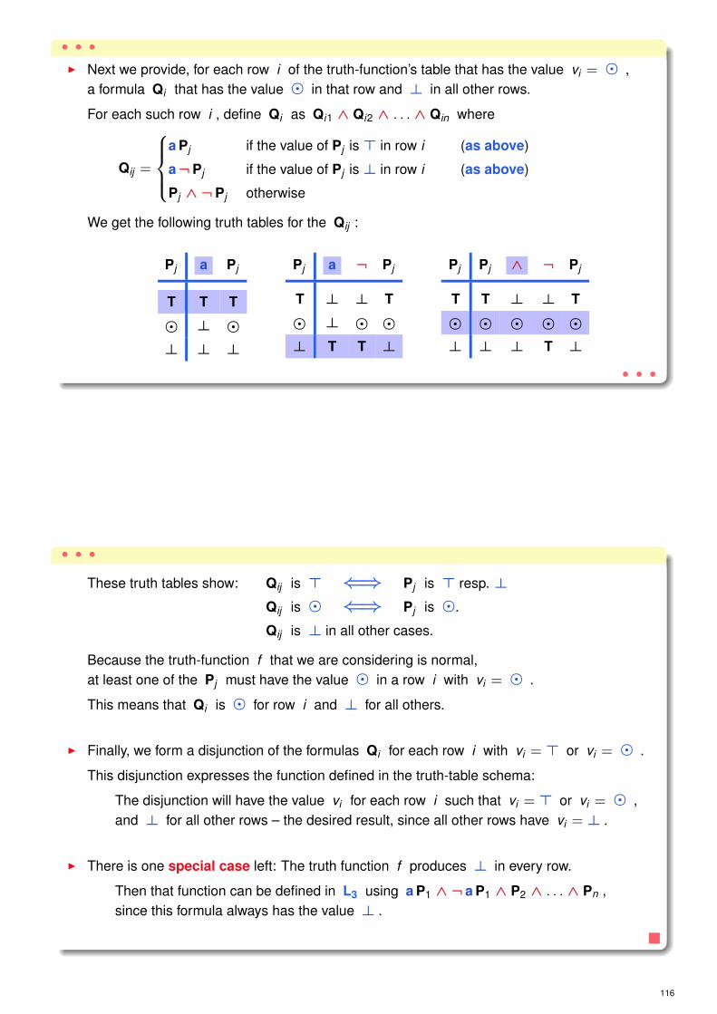
I We will first provide, for each row i of the truth-function’s table with vi = > ,

a formula Qi that has the value > in that row and ⊥ in all other rows.

. We’ll be using the connective a , which is definable in L3 : ( a P ≡ ¬(P→¬P)

. For each such row of the table, we define Qi as Qi1 ∧ Qi2 ∧ . . . ∧ Qin where

Qij =

a Pj if the value of Pj is> in row i

a¬Pj if the value of Pj is⊥ in row i

¬ a Pj ∧ ¬ a¬Pj otherwise

. Each of these formulas Qij defined for a particular row i

will have the value > when Pj has the value it has in row i

and will have the value ⊥ otherwise

as can be seen with the following truth tables for the Qij :

• • •

• • •

Pj a Pj

T T T

� ⊥ �⊥ ⊥ ⊥

Pj a ¬ Pj

T ⊥ ⊥ T

� ⊥ � �⊥ T T ⊥

Pj ¬ a Pj ∧ ¬ a ¬ Pj

T ⊥ T T ⊥ T ⊥ ⊥ T

� T ⊥ � T T ⊥ � �⊥ T ⊥ ⊥ ⊥ ⊥ T T ⊥

These truth tables show: Qij is > ⇐⇒ Pj is > , ⊥ resp. � .

Qij is ⊥ in all other cases.

So the conjunction Qi will have the value > in the row i for which it is defined,

but will be false in each other row

since it will have at least one conjunct with the value ⊥ .• • •

Example:

(n = 4)

P1 P2 P3 P4 @(P1, . . . ,P4)

......

......

...T T ⊥ � >...

......

......

a P1

∧ a P2

∧ a¬P3

∧ ¬ a P4 ∧ ¬ a¬P4

114

• • •

I Next we provide, for each row i of the truth-function’s table that has the value vi = � ,a formula Qi that has the value � in that row and ⊥ in all other rows.

For each such row i , define Qi as Qi1 ∧ Qi2 ∧ . . . ∧ Qin where

Qij =

a Pj if the value of Pj is> in row i (as above)

a¬Pj if the value of Pj is⊥ in row i (as above)

Pj ∧ ¬Pj otherwise

We get the following truth tables for the Qij :

Pj a Pj

T T T

� ⊥ �⊥ ⊥ ⊥

Pj a ¬ Pj

T ⊥ ⊥ T

� ⊥ � �⊥ T T ⊥

Pj Pj ∧ ¬ Pj

T T ⊥ ⊥ T

� � � � �⊥ ⊥ ⊥ T ⊥

• • •

• • •

These truth tables show: Qij is > ⇐⇒ Pj is > resp. ⊥Qij is � ⇐⇒ Pj is �.

Qij is ⊥ in all other cases.

Because the truth-function f that we are considering is normal,at least one of the Pj must have the value � in a row i with vi = � .

This means that Qi is � for row i and ⊥ for all others.

I Finally, we form a disjunction of the formulas Qi for each row i with vi = > or vi = � .

This disjunction expresses the function defined in the truth-table schema:

The disjunction will have the value vi for each row i such that vi = > or vi = � ,and ⊥ for all other rows – the desired result, since all other rows have vi = ⊥ .

I There is one special case left: The truth function f produces ⊥ in every row.

Then that function can be defined in L3 using a P1 ∧ ¬ a P1 ∧ P2 ∧ . . . ∧ Pn ,since this formula always has the value ⊥ .

116

Example 2.13Build the formula corresponding the the connective given by the following truth table

P Q P # Q

T T T

T � �T ⊥ T

� T T

� � �� ⊥ �⊥ T ⊥⊥ � �⊥ ⊥ ⊥

(a P ∧ a Q)

∨ ((a P ∧ (Q ∧ ¬Q))

∨ ((a P ∧ a¬Q)

∨ (((¬ a P ∧ ¬ a¬P) ∧ a Q)

∨ (((P ∧ ¬P) ∧ (Q ∧ ¬Q))

∨ (((P ∧ ¬P) ∧ a¬Q)

∨ (a¬P ∧ (Q ∧ ¬Q)))))))

For the generated formula we get the truth table on the next slide.(The leftmost ∨ is the main connective)

P Q P#Q (a P∧ a Q) ∨ ((a P∧(Q ∧¬ Q)) ∨ ((a P∧ a ¬ Q) ∨ (((¬ a P∧¬ a ¬ P)∧ a Q) ∨ · · ·

T T T T T T T T T T T⊥ T ⊥⊥ T ⊥ T T⊥⊥⊥ T ⊥ ⊥T T⊥T⊥⊥ T ⊥T T ⊥ · · ·T� � T T⊥⊥� � T T�� T T⊥⊥�� ⊥ ⊥T T⊥T⊥⊥ T ⊥⊥� ⊥ · · ·T⊥ T T T⊥⊥⊥ T T T⊥⊥⊥T ⊥ T T T T T T ⊥ T ⊥T T⊥T⊥⊥ T ⊥⊥⊥ ⊥ · · ·� T T ⊥�⊥T T T ⊥ �⊥ T ⊥⊥ T T ⊥ �⊥⊥⊥ T T T⊥�T T⊥�� T T T T · · ·�� ⊥�⊥⊥� � ⊥ �⊥�� ⊥ �⊥⊥�� T⊥�T T⊥��⊥⊥� � · · ·�⊥ � ⊥�⊥⊥⊥ � ⊥ �⊥⊥⊥T ⊥ � ⊥ �⊥T T ⊥ � T⊥�T T⊥��⊥⊥⊥ � · · ·⊥ T ⊥ ⊥⊥⊥T T ⊥ ⊥ ⊥⊥ T ⊥⊥ T ⊥ ⊥ ⊥⊥⊥⊥ T ⊥ T⊥⊥⊥⊥T T ⊥⊥T T ⊥ · · ·⊥� � ⊥⊥⊥⊥� � ⊥ ⊥⊥�� ⊥ ⊥⊥⊥�� T⊥⊥⊥⊥T T ⊥⊥⊥� � · · ·⊥⊥ ⊥ ⊥⊥⊥⊥⊥ ⊥ ⊥ ⊥⊥⊥⊥T ⊥ ⊥ ⊥ ⊥⊥T T ⊥ ⊥ T⊥⊥⊥⊥T T ⊥⊥⊥⊥ ⊥ · · ·

· · · ∨ ((( P ∧¬ P)∧(Q ∧¬ Q)) ∨ ((( P ∧¬ P)∧ a ¬ Q) ∨ (a ¬ P ∧(Q ∧¬Q )))))))

· · · ⊥ T⊥⊥ T ⊥ T ⊥⊥ T ⊥ T⊥⊥ T ⊥⊥⊥ T ⊥ ⊥⊥ T⊥ T ⊥⊥ T

· · · ⊥ T⊥⊥ T ⊥�� ⊥ T⊥⊥ T ⊥⊥�� ⊥ ⊥⊥ T⊥��· · · ⊥ T⊥⊥ T ⊥⊥⊥ T ⊥ ⊥ T⊥⊥ T ⊥ T T ⊥ ⊥ ⊥⊥ T⊥⊥⊥ T⊥· · · T ��⊥ T ⊥⊥ T ⊥ ��⊥⊥⊥ T ⊥ ⊥��⊥ T ⊥⊥ T

· · · � �� ⊥⊥�� ⊥��⊥��· · · � ��⊥⊥⊥ T ⊥ � �� T T ⊥ � ⊥��⊥⊥⊥ T⊥· · · ⊥ ⊥⊥ T ⊥⊥ T ⊥⊥ T ⊥ ⊥⊥ T ⊥⊥⊥⊥ T ⊥ T T⊥⊥ T ⊥⊥ T

· · · � ⊥⊥ T ⊥⊥�� ⊥ ⊥⊥ T ⊥⊥⊥�� T T⊥��· · · ⊥ ⊥⊥ T ⊥⊥⊥⊥ T ⊥ ⊥ ⊥⊥ T ⊥⊥ T T ⊥ ⊥ T T⊥⊥⊥⊥ T⊥

118

Theorem 2.14

No non-normal connective is definable in L3 (with the standard connectives).

Consequently, the standard set of connectives of L3 is not complete.

ProofAll of the L3 connectives are normal,so it is impossible to produce a formula that has the value �when all of its constituents have values > or ⊥ .

Remark 2.15We don’t consider it a bad thing that non-normal truth-functions cannot be defined in L3 ,for it is hard to come up with an examplewhere we would want a connective to produce a non-classical valuebased on classical values alone for its constituents.


DEFINING NON-NORMAL CONNECTIVES

Jerzy Słupecki1904 – 1987

Tertium operator ([Słupecki, 1936])

P T P

T �� ⊥ �

Słupecki’s Theorem

Extending the standard connectivesof L3 by the T connectiveresults in a complete set of connectives.

([Słupecki, 1936])

122

Definition 2.16

The Słupecki operator T allows for the definition of a neutral truth constant:

n = T p1

We may also define truth constants t and f for the other truth values:

t = p1→ p1

f = ¬(p1→ p1)

Remark 2.17

Definition 2.16 implies that for all interpetations I holds: nI = �

tI = >fI = ⊥

Lemma 2.18

The standard connectives of L3 augmented by the Słupecki operator Tconstitute a complete set of 3-valued connectives.

ProofGiven a n-ary connective ◦ of 3-valued logic.

We show that there is a formula G with at most the propositional variables p1, . . . ,pn

such that ◦ (p1, . . . ,pn) ≡ G .

Note: Replacing all occurrences of pn in G by t , n or f ,we obtain three formulae G> , G� and G⊥ respectively,which define the respective (n-1)-ary connectives ◦> , ◦� and ◦⊥ .

Proof by mathematical induction on n .

I.B. n = 0 : ◦ is identical to one of the truth constants.

I.H. For an n-ary connective ◦we assume that there are formulae G⊥,G� and G>which define the (n-1)-ary connectives ◦> , ◦� and ◦⊥ .i.e., such that

G⊥ ≡ ◦⊥ (p1, ...,pn−1) := ◦ (p1, ...,pn−1, f)

G� ≡ ◦� (p1, ...,pn−1) := ◦ (p1, ...,pn−1,n)

G> ≡ ◦> (p1, ...,pn−1) := ◦ (p1, ...,pn−1, t)

• • •

124

• • •

I.S. We define the following auxiliary formulae A> := a pn

A⊥ := a¬pn

A� := ∼pn ∧ ∼¬pn

whose interpretations are given by the following table

(see also next slide)

pn A> A� A⊥

T T ⊥ ⊥� ⊥ T ⊥⊥ ⊥ ⊥ T

And we define G := (G⊥ ∧ A⊥) ∨ (G� ∧ A�) ∨ (G> ∧ A>) .

Consider the disjunct (G⊥ ∧ A⊥) ≡ ◦ (p1, ...,pn−1, f) ∧ A⊥. If pn is ⊥ , then A⊥ is > and ◦ (p1, ...,pn−1, f) is ◦ (p1, ...,pn−1,pn). Otherwise, A⊥ is ⊥ and the value of G is determined by the other disjuncts

The other two disjuncts can be analyzed analogously.

Thus we obtain G ≡ ◦ (p1, . . . ,pn) .

A>: F a F

T T T

� ⊥ �⊥ ⊥ ⊥

A�: F ∼ F ∧ ∼ ¬ F

T ⊥ T ⊥ T ⊥ T

� T � T T � �⊥ T ⊥ ⊥ ⊥ T ⊥

A⊥: F a ¬ F

T ⊥ ⊥ T

� ⊥ � �⊥ T T ⊥

126

Example 2.19

Given the non-normal unary connective . F .F

T �� ⊥⊥ �

We get the 0-ary ‘connectives’ (constants) G> ≡ .> := . t ( ≡ n )

G� ≡ .� := .n ( ≡ f )

G⊥ ≡ .⊥ := . f ( ≡ n )

According to the construction in the proof, we get

.F ≡ (.⊥ ∧ A⊥) ∨ (.� ∧ A�) ∨ (.> ∧ A>)

≡ (n ∧ a F) ∨ (f ∧ ∼F ∧ ∼¬F) ∨ (n ∧ a¬F)

We can immediately drop the middle conjunct and obtain

.F ≡ (n ∧ a F) ∨ (n ∧ a¬F)

Distributivity of ∧ and ∨ yields: .F ≡ n ∧ (a F ∨ a¬F)

• • •

• • •

The correctness of the simplification is verfied by the following truth tables:

F n ∧ (a F ∨ a ¬ F) ≡ (n ∧ a F) ∨ ((f ∧ (∼ F ∧ ∼ ¬ F)) ∨ (n ∧ a ¬ F))

T � � T T T ⊥⊥ T T � � T T � ⊥ ⊥ ⊥ T ⊥ T ⊥ T ⊥ � ⊥⊥⊥ T

� � ⊥ ⊥ �⊥⊥� � T � ⊥⊥ � ⊥ ⊥ ⊥ T � T T � � ⊥ � ⊥⊥� �⊥ � � ⊥ ⊥ T T T ⊥ T � ⊥⊥ ⊥ � ⊥ ⊥ T ⊥⊥⊥ T ⊥ � � � T T ⊥

The green columns show the definition of .F .

128

Example 2.20

Given a binary connective ◦ whose associated truth function is given by the following table

T � ⊥

T ⊥ � ⊥� � � �⊥ ⊥ � ⊥

Obviously, we can represent

G> ≡ A ◦ t ≡ A ∧ ¬A (1. column)

G� ≡ A ◦ n ≡ n (2. column)

G⊥ ≡ A ◦ f ≡ A ∧ ¬A (3. column)

According to the construction in the proof, we get

A ◦ B ≡ (G> ∧ A>) ∨ (G� ∧ A�) ∨ (G⊥ ∧ A⊥)

≡ (A ∧ ¬A ∧ a B) ∨ (n ∧ ∼B ∧ ∼¬B) ∨ (A ∧ ¬A ∧ a¬B)• • •

• • •

I With distributivity of ∧ and ∨ we get from the first and the last conjunct

(A ∧ ¬A) ∨ (a B ∧ a¬B)

However, a B ∧ a¬B is always ⊥ , since B and ¬B cannot be both > .

I With the idempotence, commutativity and associativity of ∧we can rewrite the middle conjunct n ∧ ∼B ∧ ∼¬B to:

(n ∧ ∼B) ∧ (n ∧ ∼¬B)

and with (n ∧ ∼P) ≡ (n ∧ ¬P) to: (n ∧ ¬B) ∧ (n ∧ ¬¬B)

We get next: n ∧ ¬B ∧ B

Since ¬B ∧ B is either ⊥ or � , the n can be dropped.

Consequently, the formula obtained for A ◦ B by our algorithm can be simplified to

A ◦ B ≡ (A ∧ ¬A) ∨ (B ∧ ¬B) (see also next slide)

130

B A (B∧¬B) ∨ (A∧¬ A) ≡ (A∧(¬A∧ a B)) ∨ ((n∧(∼B∧∼¬B))∨ (A∧(¬A∧ a ¬B)))

T T T⊥⊥ T ⊥ T⊥⊥ T T T⊥⊥ T⊥ T T ⊥ �⊥ ⊥ T⊥ T⊥ T ⊥ T⊥⊥ T⊥⊥⊥ T

T� T⊥⊥ T � �� T �� T T � �⊥ ⊥ T⊥ T⊥ T ⊥�⊥��⊥⊥⊥ T

T⊥ T⊥⊥ T ⊥ ⊥⊥ T⊥ T ⊥⊥ T⊥ T T T ⊥ �⊥ ⊥ T⊥ T⊥ T ⊥⊥⊥ T⊥⊥⊥⊥ T

� T �� T⊥⊥ T T T⊥⊥ T⊥⊥� � �� T � T T�� T⊥⊥ T⊥⊥��

�� T �⊥��⊥⊥� � �� T � T T�� ⊥��⊥⊥��

�⊥ �� ⊥⊥ T⊥ T ⊥⊥ T⊥⊥⊥� � �� T � T T�� ⊥⊥ T⊥⊥⊥��

⊥ T ⊥⊥ T⊥ ⊥ T⊥⊥ T T T⊥⊥ T⊥⊥⊥ ⊥ �⊥ T ⊥⊥⊥ T ⊥ ⊥ T⊥⊥ T⊥ T T ⊥⊥� ⊥⊥ T⊥ � �� T �⊥��⊥⊥⊥ � �⊥ T ⊥⊥⊥ T ⊥ �� T T ⊥

⊥⊥ ⊥⊥ T⊥ ⊥ ⊥⊥ T⊥ T ⊥⊥ T⊥⊥⊥⊥ ⊥ �⊥ T ⊥⊥⊥ T ⊥ ⊥⊥⊥ T⊥ T T T ⊥

Example 2.21

Given the binary connective ∧BI T � ⊥

T T � ⊥� � � �⊥ ⊥ � ⊥

We can represent A ∧BI t ≡ A (1. column)

A ∧BI n ≡ n (2. column)

A ∧BI f ≡ ¬A ∧ A (3. column)

From which we obtain according to the construction in the proof

A ∧BI B ≡ (A ∧ a B) ∨ (n ∧ ∼B ∧ ∼¬B) ∨ (¬A ∧ A ∧ a¬B)

As with Example 2.20 we can simplify the the middle conjunct to B ∧ ¬B which yields

A ∧BI B ≡ (A ∧ a B) ∨ (B ∧ ¬B) ∨ (¬A ∧ A ∧ a¬B)

This can be further simplified to

(A ∧ B) ∨ (A ∧ ¬A) ∨ (B ∧ ¬B) (see also next slide)

which is the formula we met already in Lemma 2.5.

132

A B A ∧BI B ≡ ((¬ A ∧ A) ∧ a ¬ B) ∨ (((n ∧∼ B) ∧∼ ¬ B) ∨ (A ∧ a B))

T T T T T T ⊥ T ⊥ T ⊥⊥⊥ T T � ⊥⊥ T ⊥ T ⊥ T T T T T T

T � T � � T ⊥ T ⊥ T ⊥⊥� � � � � T � � T � � � T ⊥⊥ �

T ⊥ T ⊥ ⊥ T ⊥ T ⊥ T ⊥ T T ⊥ ⊥ � � T ⊥ ⊥⊥ T ⊥ ⊥ T ⊥⊥ ⊥� T � � T T � �� ⊥⊥⊥ T � � ⊥⊥ T ⊥ T ⊥ T � � � T T

�� T � �� ⊥⊥� � � � � T � � T � � � � ⊥⊥ �

�⊥ � � ⊥ T � �� T T ⊥ � � � T ⊥ ⊥⊥ T ⊥ ⊥ � ⊥⊥ ⊥

⊥ T ⊥ ⊥ T T T ⊥⊥ ⊥ ⊥⊥⊥ T ⊥ � ⊥⊥ T ⊥ T ⊥ T ⊥ ⊥ ⊥ T T

⊥� ⊥ � � T T ⊥⊥ ⊥ ⊥⊥� � � � � T � � T � � � ⊥ ⊥⊥ �

⊥⊥ ⊥ ⊥ ⊥ T T ⊥⊥ ⊥ ⊥ T T ⊥ ⊥ � � T ⊥ ⊥⊥ T ⊥ ⊥ ⊥ ⊥⊥ ⊥


BOLD CONNECTIVES

Definition 2.22We define two new connectiveswhich are called bold conjunction and bold disjunction (in symbols: & resp. ∇ )

P & Q := ¬(P→¬Q)

P∇ Q := ¬P→ Q

The bold connectives have the following truth-tables in L3 :

Bold Conjunction v &? w

v \ w T � ⊥

T T � ⊥� � ⊥ ⊥⊥ ⊥ ⊥ ⊥

Bold Disjunction v ∇? w

v \ w T � ⊥

T T T T

� T T �⊥ T � ⊥

Recall: ∧ and ∨ both have the value � in the ‘blue’ position.

Other Names: strong conjunction/disjunction (in contrast to the weak connectives ∧ and ∨ )

Remark 2.23The weak operators are called such because

they do not preserve the relationships of excluded middle and excluded contradiction,whereas the strong operators are called such because they do preserve those relationships.

Lemma 2.24Using the bold connectives, we have tautologies in L3

that are versions of the Law of the Excluded Middle and the Law of Non-Contradiction:

P∇ ¬P and ¬(P & ¬P) .

Proof

P ¬ (P & ¬ P)

T T T ⊥ ⊥ T

� T � ⊥ � �⊥ T ⊥ ⊥ T ⊥

P P ∇ ¬ P

T T T ⊥ T

� � T � �⊥ ⊥ T T ⊥

136

Remark 2.25Rather than define the bold connectives as we did,

we could also take them as primitive (together with ¬ )and define the L3 conditional using either of these connectives:

P→ Q := ¬(P & ¬Q) or P→ Q := ¬P∇ Q

P Q P→ Q ¬ (P & ¬ Q) ¬ P ∇ Q

T T T T T ⊥ ⊥ T ⊥ T T T

T � � � T � � � ⊥ T � �

T ⊥ ⊥ ⊥ T T T ⊥ ⊥ T ⊥ ⊥� T T T � ⊥ ⊥ T � � T T

� � T T � ⊥ � � � � T �� ⊥ � � � � T ⊥ � � � ⊥

⊥ T T T ⊥ ⊥ ⊥ T T ⊥ T T

⊥ � T T ⊥ ⊥ � � T ⊥ T �⊥ ⊥ T T ⊥ ⊥ T ⊥ T ⊥ T ⊥

Remark 2.26We may also define the biconditional P↔ Qvia the bold conjunction of the conditionals P→ Q and P← Q .

P Q (P → Q) & (Q → P) P↔ Q

T T T T T T T T T T

T � T � � � � T T �

T ⊥ T ⊥ ⊥ ⊥ ⊥ T T ⊥� T � T T � T � � �

� � � T � T � T � T

� ⊥ � � ⊥ � ⊥ T � �

⊥ T ⊥ T T ⊥ T ⊥ ⊥ ⊥⊥ � ⊥ T � � � � ⊥ �

⊥ ⊥ ⊥ T ⊥ T ⊥ T ⊥ T

138

IDEMPOTENCE

Remark 2.27Bold Connectives are NOT idempotent!

P P ≡ (P & P)

T T T T T T

� � ⊥ � ⊥ �⊥ ⊥ T ⊥ ⊥ ⊥

P P ≡ (P ∇ P)

T T T T T T

� � ⊥ � T �⊥ ⊥ T ⊥ ⊥ ⊥

However, the following holds:

P (P & P) ≡ (P & (P & P))

T T T T T T T T T T

� � ⊥ � T � ⊥ � ⊥ �⊥ ⊥ ⊥ ⊥ T ⊥ ⊥ ⊥ ⊥ ⊥

P (P ∇ P) ≡ (P ∇ (P ∇ P))

T T T T T T T T T T

� � T � T � T � T �⊥ ⊥ ⊥ ⊥ T ⊥ ⊥ ⊥ ⊥ ⊥

Remark 2.28

With & we obtain the theorem (P & (P→ Q))→ Q .

However, (P ∧ (P→ Q))→ Q is no theorem in L3 .

P Q (P & (P → Q)) → Q (P ∧ (P → Q)) → Q

T T T T T T T T T T T T T T T T

T � T � T � � T � T � T � � T �T ⊥ T ⊥ T ⊥ ⊥ T ⊥ T ⊥ T ⊥ ⊥ T ⊥� T � � � T T T T � � � T T T T

� � � � � T � T � � � � T � T �� ⊥ � ⊥ � � ⊥ T ⊥ � � � � ⊥ � ⊥⊥ T ⊥ ⊥ ⊥ T T T T ⊥ ⊥ ⊥ T T T T

⊥ � ⊥ ⊥ ⊥ T � T � ⊥ ⊥ ⊥ T � T �⊥ ⊥ ⊥ ⊥ ⊥ T ⊥ T ⊥ ⊥ ⊥ ⊥ T ⊥ T ⊥

140

Import-Export rules: (P→ (R→ Q)) ≡ ((P & R)→ Q)

P Q R (P → (R → Q)) ≡ ((P & R) → Q)

T T T T T T T T T T T T T TT T � T T � T T T T � � T TT T ⊥ T T ⊥ T T T T ⊥ ⊥ T TT � T T � T � � T T T T � �T � � T T � T � T T � � T �T � ⊥ T T ⊥ T � T T ⊥ ⊥ T �T ⊥ T T ⊥ T ⊥ ⊥ T T T T ⊥ ⊥T ⊥ � T � � � ⊥ T T � � � ⊥T ⊥ ⊥ T T ⊥ T ⊥ T T ⊥ ⊥ T ⊥� T T � T T T T T � � T T T� T � � T � T T T � ⊥ � T T� T ⊥ � T ⊥ T T T � ⊥ ⊥ T T� � T � T T � � T � � T T �� T � T � T � ⊥ � T �� ⊥ � T ⊥ T � T � ⊥ ⊥ T �� ⊥ T � � T ⊥ ⊥ T � � T � ⊥� ⊥ � � T � � ⊥ T � ⊥ � T ⊥� ⊥ ⊥ � T ⊥ T ⊥ T � ⊥ ⊥ T ⊥⊥ T T ⊥ T T T T T ⊥ ⊥ T T T⊥ T � ⊥ T � T T T ⊥ ⊥ � T T⊥ T ⊥ ⊥ T ⊥ T T T ⊥ ⊥ ⊥ T T⊥ � T ⊥ T T � � T ⊥ ⊥ T T �⊥ � � ⊥ T � T � T ⊥ ⊥ � T �⊥ � ⊥ ⊥ T ⊥ T � T ⊥ ⊥ ⊥ T �⊥ ⊥ T ⊥ T T ⊥ ⊥ T ⊥ ⊥ T T ⊥⊥ ⊥ � ⊥ T � � ⊥ T ⊥ ⊥ � T ⊥⊥ ⊥ ⊥ ⊥ T ⊥ T ⊥ T ⊥ ⊥ ⊥ T ⊥

However

P Q R (P → (R → Q)) → ((P ∧ R) → Q)

T T T T T T T T T T T T T TT T � T T � T T T T � � T TT T ⊥ T T ⊥ T T T T ⊥ ⊥ T TT � T T � T � � T T T T � �T � � T T � T � T T � � T �T � ⊥ T T ⊥ T � T T ⊥ ⊥ T �T ⊥ T T ⊥ T ⊥ ⊥ T T T T ⊥ ⊥T ⊥ � T � � � ⊥ T T � � � ⊥T ⊥ ⊥ T T ⊥ T ⊥ T T ⊥ ⊥ T ⊥� T T � T T T T T � � T T T� T � � T � T T T � � � T T� T ⊥ � T ⊥ T T T � ⊥ ⊥ T T� � T � T T � � T � � T T �� T � T � T � � � T �� ⊥ � T ⊥ T � T � ⊥ ⊥ T �� ⊥ T � � T ⊥ ⊥ T � � T � ⊥� ⊥ � � T � � ⊥ � � � � � ⊥� ⊥ ⊥ � T ⊥ T ⊥ T � ⊥ ⊥ T ⊥⊥ T T ⊥ T T T T T ⊥ ⊥ T T T⊥ T � ⊥ T � T T T ⊥ ⊥ � T T⊥ T ⊥ ⊥ T ⊥ T T T ⊥ ⊥ ⊥ T T⊥ � T ⊥ T T � � T ⊥ ⊥ T T �⊥ � � ⊥ T � T � T ⊥ ⊥ � T �⊥ � ⊥ ⊥ T ⊥ T � T ⊥ ⊥ ⊥ T �⊥ ⊥ T ⊥ T T ⊥ ⊥ T ⊥ ⊥ T T ⊥⊥ ⊥ � ⊥ T � � ⊥ T ⊥ ⊥ � T ⊥⊥ ⊥ ⊥ ⊥ T ⊥ T ⊥ T ⊥ ⊥ ⊥ T ⊥

142

But this direction holds

P Q R ((P ∧ R) → Q) → (P → (R → Q))

T T T T T T T T T T T T T TT T � T � � T T T T T � T TT T ⊥ T ⊥ ⊥ T T T T T ⊥ T TT � T T T T � � T T � T � �T � � T � � T � T T T � T �T � ⊥ T ⊥ ⊥ T � T T T ⊥ T �T ⊥ T T T T ⊥ ⊥ T T ⊥ T ⊥ ⊥T ⊥ � T � � � ⊥ T T � � � ⊥T ⊥ ⊥ T ⊥ ⊥ T ⊥ T T T ⊥ T ⊥� T T � � T T T T � T T T T� T � � � � T T T � T � T T� T ⊥ � ⊥ ⊥ T T T � T ⊥ T T� � T � � T T � T � T T � �� T � T � T � T �� ⊥ � ⊥ ⊥ T � T � T ⊥ T �� ⊥ T � � T � ⊥ T � � T ⊥ ⊥� ⊥ � � � � � ⊥ T � T � � ⊥� ⊥ ⊥ � ⊥ ⊥ T ⊥ T � T ⊥ T ⊥⊥ T T ⊥ ⊥ T T T T ⊥ T T T T⊥ T � ⊥ ⊥ � T T T ⊥ T � T T⊥ T ⊥ ⊥ ⊥ ⊥ T T T ⊥ T ⊥ T T⊥ � T ⊥ ⊥ T T � T ⊥ T T � �⊥ � � ⊥ ⊥ � T � T ⊥ T � T �⊥ � ⊥ ⊥ ⊥ ⊥ T � T ⊥ T ⊥ T �⊥ ⊥ T ⊥ ⊥ T T ⊥ T ⊥ T T ⊥ ⊥⊥ ⊥ � ⊥ ⊥ � T ⊥ T ⊥ T � � ⊥⊥ ⊥ ⊥ ⊥ ⊥ ⊥ T ⊥ T ⊥ T ⊥ T ⊥

COMPARING BOLD AND WEAK CONJUNCTION

P Q (P & Q) → (P ∧ Q)

T T T T T T T T T

T � T � � T T � �T ⊥ T ⊥ ⊥ T T ⊥ ⊥� T � � T T � � T

� � � ⊥ � T � � �� ⊥ � ⊥ ⊥ T � ⊥ ⊥⊥ T ⊥ ⊥ T T ⊥ ⊥ T

⊥ � ⊥ ⊥ � T ⊥ ⊥ �⊥ ⊥ ⊥ ⊥ ⊥ T ⊥ ⊥ ⊥

P Q (P ∧ Q) → (P & Q)

T T T T T T T T T

T � T � � T T � �T ⊥ T ⊥ ⊥ T T ⊥ ⊥� T � � T T � � T

� � � � � � � ⊥ �� ⊥ � ⊥ ⊥ T � ⊥ ⊥⊥ T ⊥ ⊥ T T ⊥ ⊥ T

⊥ � ⊥ ⊥ � T ⊥ ⊥ �⊥ ⊥ ⊥ ⊥ ⊥ T ⊥ ⊥ ⊥

P Q (P ∨ Q) → (P ∇ Q)

T T T T T T T T T

T � T T � T T T �T ⊥ T T ⊥ T T T ⊥� T � T T T � T T

� � � � � T � T �� ⊥ � � ⊥ T � � ⊥⊥ T ⊥ T T T ⊥ T T

⊥ � ⊥ � � T ⊥ � �⊥ ⊥ ⊥ ⊥ ⊥ T ⊥ ⊥ ⊥

P Q (P ∇ Q) → (P ∨ Q)

T T T T T T T T T

T � T T � T T T �T ⊥ T T ⊥ T T T ⊥� T � T T T � T T

� � � T � � � � �� ⊥ � � ⊥ T � � ⊥⊥ T ⊥ T T T ⊥ T T

⊥ � ⊥ � � T ⊥ � �⊥ ⊥ ⊥ ⊥ ⊥ T ⊥ ⊥ ⊥

144

WHICH CLASSICAL TAUTOLOGIES (DON’T) HOLD?

Formulae with blue background don’t hold.

(P ∨ Q) ≡ (Q ∨ P) (P∇ Q) ≡ (Q∇ P)

(P ∧ Q) ≡ (Q ∧ P) (P & Q) ≡ (Q & P)

(P ∨ (Q ∨ R)) ≡ ((P ∨ Q) ∨ R) (P∇ (Q∇ R)) ≡ ((P∇ Q)∇ R)

(P ∧ (Q ∧ R)) ≡ ((P ∧ Q) ∧ R) (P & (Q & R)) ≡ ((P & Q) & R)

P→ (P ∨ Q) P→ (P∇ Q)

P→ (Q→ (P ∧ Q)) P→ (Q→ (P & Q))

(P ∧ Q)→ P (P & Q)→ P

¬(P ∧ Q) ≡ (¬P ∨ ¬Q) ¬(P & Q) ≡ (¬P∇ ¬Q)

¬(P & Q) → (¬P ∨ ¬Q) ¬(P & Q) ← (¬P ∨ ¬Q)

¬(P ∧ Q) → (¬P∇ ¬Q) ¬(P ∧ Q) ← (¬P∇ ¬Q)

¬(P∇ Q) → (¬P ∧ ¬Q) ¬(P∇ Q) ← (¬P ∧ ¬Q)

¬(P ∨ Q) → (¬P & ¬Q) ¬(P ∨ Q) ← (¬P & ¬Q)

(P ∧ (Q ∨ R)) ≡ ((P ∧ Q) ∨ (P ∧ R)) (P ∨ (Q ∧ R)) ≡ ((P ∨ Q) ∧ (P ∨ R))

(P & (Q∇ R)) → ((P & Q)∇ (P & R)) (P & (Q∇ R)) ← ((P & Q)∇ (P & R))

(P∇ (Q & R)) → ((P∇ Q) & (P∇ R)) (P∇ (Q & R)) ← ((P∇ Q) & (P∇ R))

(P ∧ (Q∇ R)) → ((P ∧ Q)∇ (P ∧ R)) (P ∧ (Q∇ R)) ← ((P ∧ Q)∇ (P ∧ R))

(P ∨ (Q & R)) → ((P ∨ Q) & (P ∨ R)) (P ∨ (Q & R)) ← ((P ∨ Q) & (P ∨ R))

(P & (Q ∨ R)) → ((P & Q) ∨ (P & R)) (P & (Q ∨ R)) ← ((P & Q) ∨ (P & R))

(P∇ (Q ∧ R)) → ((P∇ Q) ∧ (P∇ R)) (P∇ (Q ∧ R)) ← ((P∇ Q) ∧ (P∇ R))

((P ∧ Q) ∨ P) ≡ P ((P ∨ Q) ∧ P) ≡ P

((P & Q)∇ P)→ P ((P∇ Q) & P)→ P

((P & Q)∇ P)← P ((P∇ Q) & P)← P

((P→ Q) ∧ (Q→ R))→ (P→ R) ((P→ Q) & (Q→ R))→ (P→ R)

146

P Q ¬ (P & Q) → (¬ P ∨ ¬ Q)

T T ⊥ T T T T ⊥ T ⊥ ⊥ TT � � T � � T ⊥ T � � �T ⊥ T T ⊥ ⊥ T ⊥ T T T ⊥� T � � � T T � � � ⊥ T� � T � ⊥ � � � � � � �� ⊥ T � ⊥ ⊥ T � � T T ⊥⊥ T T ⊥ ⊥ T T T ⊥ T ⊥ T⊥ � T ⊥ ⊥ � T T ⊥ T � �⊥ ⊥ T ⊥ ⊥ ⊥ T T ⊥ T T ⊥

P Q ¬ (P ∧ Q) ← (¬ P ∇ ¬ Q)

T T ⊥ T T T T ⊥ T ⊥ ⊥ TT � � T � � T ⊥ T � � �T ⊥ T T ⊥ ⊥ T ⊥ T T T ⊥� T � � � T T � � � ⊥ T� � � � � � � � � T � �� ⊥ T � ⊥ ⊥ T � � T T ⊥⊥ T T ⊥ ⊥ T T T ⊥ T ⊥ T⊥ � T ⊥ ⊥ � T T ⊥ T � �⊥ ⊥ T ⊥ ⊥ ⊥ T T ⊥ T T ⊥

P Q ¬ (P ∇ Q) ← (¬ P ∧ ¬ Q)

T T ⊥ T T T T ⊥ T ⊥ ⊥ TT � ⊥ T T � T ⊥ T ⊥ � �T ⊥ ⊥ T T ⊥ T ⊥ T ⊥ T ⊥� T ⊥ � T T T � � ⊥ ⊥ T� � ⊥ � T � � � � � � �� ⊥ � � � ⊥ T � � � T ⊥⊥ T ⊥ ⊥ T T T T ⊥ ⊥ ⊥ T⊥ � � ⊥ � � T T ⊥ � � �⊥ ⊥ T ⊥ ⊥ ⊥ T T ⊥ T T ⊥

P Q ¬ (P ∨ Q) → (¬ P & ¬ Q)

T T ⊥ T T T T ⊥ T ⊥ ⊥ TT � ⊥ T T � T ⊥ T ⊥ � �T ⊥ ⊥ T T ⊥ T ⊥ T ⊥ T ⊥� T ⊥ � T T T � � ⊥ ⊥ T� � � � � � � � � ⊥ � �� ⊥ � � � ⊥ T � � � T ⊥⊥ T ⊥ ⊥ T T T T ⊥ ⊥ ⊥ T⊥ � � ⊥ � � T T ⊥ � � �⊥ ⊥ T ⊥ ⊥ ⊥ T T ⊥ T T ⊥

148

P Q R (P & (Q ∇ R)) → ((P & Q) ∇ (P & R))

T T T T T T T T T T T T T T T TT T � T T T T � T T T T T T � �T T ⊥ T T T T ⊥ T T T T T T ⊥ ⊥T � T T T � T T T T � � T T T TT � � T T � T � T T � � T T � �T � ⊥ T � � � ⊥ T T � � � T ⊥ ⊥T ⊥ T T T ⊥ T T T T ⊥ ⊥ T T T TT ⊥ � T � ⊥ � � T T ⊥ ⊥ � T � �T ⊥ ⊥ T ⊥ ⊥ ⊥ ⊥ T T ⊥ ⊥ ⊥ T ⊥ ⊥� T T � � T T T T � � T T � � T� T � � � T T � T � � T � � ⊥ �� T ⊥ � � T T ⊥ T � � T � � ⊥ ⊥� � T � � � T T T � ⊥ � � � � T� � � � � � T � � � ⊥ � ⊥ � ⊥ �� ⊥ � ⊥ � � ⊥ T � ⊥ � ⊥ � ⊥ ⊥� ⊥ T � � ⊥ T T T � ⊥ ⊥ � � � T� ⊥ � � ⊥ ⊥ � � T � ⊥ ⊥ ⊥ � ⊥ �� ⊥ ⊥ � ⊥ ⊥ ⊥ ⊥ T � ⊥ ⊥ ⊥ � ⊥ ⊥⊥ T T ⊥ ⊥ T T T T ⊥ ⊥ T ⊥ ⊥ ⊥ T⊥ T � ⊥ ⊥ T T � T ⊥ ⊥ T ⊥ ⊥ ⊥ �⊥ T ⊥ ⊥ ⊥ T T ⊥ T ⊥ ⊥ T ⊥ ⊥ ⊥ ⊥⊥ � T ⊥ ⊥ � T T T ⊥ ⊥ � ⊥ ⊥ ⊥ T⊥ � � ⊥ ⊥ � T � T ⊥ ⊥ � ⊥ ⊥ ⊥ �⊥ � ⊥ ⊥ ⊥ � � ⊥ T ⊥ ⊥ � ⊥ ⊥ ⊥ ⊥⊥ ⊥ T ⊥ ⊥ ⊥ T T T ⊥ ⊥ ⊥ ⊥ ⊥ ⊥ T⊥ ⊥ � ⊥ ⊥ ⊥ � � T ⊥ ⊥ ⊥ ⊥ ⊥ ⊥ �⊥ ⊥ ⊥ ⊥ ⊥ ⊥ ⊥ ⊥ T ⊥ ⊥ ⊥ ⊥ ⊥ ⊥ ⊥

P Q R (P & (Q ∇ R)) ← ((P & Q) ∇ (P & R))

T T T T T T T T T T T T T T T TT T � T T T T � T T T T T T � �T T ⊥ T T T T ⊥ T T T T T T ⊥ ⊥T � T T T � T T T T � � T T T TT � � T T � T � T T � � T T � �T � ⊥ T � � � ⊥ T T � � � T ⊥ ⊥T ⊥ T T T ⊥ T T T T ⊥ ⊥ T T T TT ⊥ � T � ⊥ � � T T ⊥ ⊥ � T � �T ⊥ ⊥ T ⊥ ⊥ ⊥ ⊥ T T ⊥ ⊥ ⊥ T ⊥ ⊥� T T � � T T T � � � T T � � T� T � � � T T � T � � T � � ⊥ �� T ⊥ � � T T ⊥ T � � T � � ⊥ ⊥� � T � � � T T T � ⊥ � � � � T� � � � � � T � T � ⊥ � ⊥ � ⊥ �� ⊥ � ⊥ � � ⊥ T � ⊥ � ⊥ � ⊥ ⊥� ⊥ T � � ⊥ T T T � ⊥ ⊥ � � � T� ⊥ � � ⊥ ⊥ � � T � ⊥ ⊥ ⊥ � ⊥ �� ⊥ ⊥ � ⊥ ⊥ ⊥ ⊥ T � ⊥ ⊥ ⊥ � ⊥ ⊥⊥ T T ⊥ ⊥ T T T T ⊥ ⊥ T ⊥ ⊥ ⊥ T⊥ T � ⊥ ⊥ T T � T ⊥ ⊥ T ⊥ ⊥ ⊥ �⊥ T ⊥ ⊥ ⊥ T T ⊥ T ⊥ ⊥ T ⊥ ⊥ ⊥ ⊥⊥ � T ⊥ ⊥ � T T T ⊥ ⊥ � ⊥ ⊥ ⊥ T⊥ � � ⊥ ⊥ � T � T ⊥ ⊥ � ⊥ ⊥ ⊥ �⊥ � ⊥ ⊥ ⊥ � � ⊥ T ⊥ ⊥ � ⊥ ⊥ ⊥ ⊥⊥ ⊥ T ⊥ ⊥ ⊥ T T T ⊥ ⊥ ⊥ ⊥ ⊥ ⊥ T⊥ ⊥ � ⊥ ⊥ ⊥ � � T ⊥ ⊥ ⊥ ⊥ ⊥ ⊥ �⊥ ⊥ ⊥ ⊥ ⊥ ⊥ ⊥ ⊥ T ⊥ ⊥ ⊥ ⊥ ⊥ ⊥ ⊥

150

P Q R (P ∇ (Q & R)) → ((P ∇ Q) & (P ∇ R))

T T T T T T T T T T T T T T T TT T � T T T � � T T T T T T T �T T ⊥ T T T ⊥ ⊥ T T T T T T T ⊥T � T T T � � T T T T � T T T TT � � T T � ⊥ � T T T � T T T �T � ⊥ T T � ⊥ ⊥ T T T � T T T ⊥T ⊥ T T T ⊥ ⊥ T T T T ⊥ T T T TT ⊥ � T T ⊥ ⊥ � T T T ⊥ T T T �T ⊥ ⊥ T T ⊥ ⊥ ⊥ T T T ⊥ T T T ⊥� T T � T T T T T � T T T � T T� T � � T T � � T � T T T � T �� T ⊥ � � T ⊥ ⊥ T � T T � � � ⊥� � T � T � � T T � T � T � T T� � � � � � ⊥ � T � T � T � T �� ⊥ � � � ⊥ ⊥ T � T � � � � ⊥� ⊥ T � � ⊥ ⊥ T T � � ⊥ � � T T� ⊥ � � � ⊥ ⊥ � T � � ⊥ � � T �� ⊥ ⊥ � � ⊥ ⊥ ⊥ � � � ⊥ ⊥ � � ⊥⊥ T T ⊥ T T T T T ⊥ T T T ⊥ T T⊥ T � ⊥ � T � � T ⊥ T T � ⊥ � �⊥ T ⊥ ⊥ ⊥ T ⊥ ⊥ T ⊥ T T ⊥ ⊥ ⊥ ⊥⊥ � T ⊥ � � � T T ⊥ � � � ⊥ T T⊥ � � ⊥ ⊥ � ⊥ � T ⊥ � � ⊥ ⊥ � �⊥ � ⊥ ⊥ ⊥ � ⊥ ⊥ T ⊥ � � ⊥ ⊥ ⊥ ⊥⊥ ⊥ T ⊥ ⊥ ⊥ ⊥ T T ⊥ ⊥ ⊥ ⊥ ⊥ T T⊥ ⊥ � ⊥ ⊥ ⊥ ⊥ � T ⊥ ⊥ ⊥ ⊥ ⊥ � �⊥ ⊥ ⊥ ⊥ ⊥ ⊥ ⊥ ⊥ T ⊥ ⊥ ⊥ ⊥ ⊥ ⊥ ⊥

P Q R (P ∇ (Q & R)) → ((P ∇ Q) & (P ∇ R))

T T T T T T T T T T T T T T T TT T � T T T � � T T T T T T T �T T ⊥ T T T ⊥ ⊥ T T T T T T T ⊥T � T T T � � T T T T � T T T TT � � T T � ⊥ � T T T � T T T �T � ⊥ T T � ⊥ ⊥ T T T � T T T ⊥T ⊥ T T T ⊥ ⊥ T T T T ⊥ T T T TT ⊥ � T T ⊥ ⊥ � T T T ⊥ T T T �T ⊥ ⊥ T T ⊥ ⊥ ⊥ T T T ⊥ T T T ⊥� T T � T T T T T � T T T � T T� T � � T T � � T � T T T � T �� T ⊥ � � T ⊥ ⊥ T � T T � � � ⊥� � T � T � � T T � T � T � T T� � � � � � ⊥ � T � T � T � T �� ⊥ � � � ⊥ ⊥ T � T � � � � ⊥� ⊥ T � � ⊥ ⊥ T T � � ⊥ � � T T� ⊥ � � � ⊥ ⊥ � T � � ⊥ � � T �� ⊥ ⊥ � � ⊥ ⊥ ⊥ � � � ⊥ ⊥ � � ⊥⊥ T T ⊥ T T T T T ⊥ T T T ⊥ T T⊥ T � ⊥ � T � � T ⊥ T T � ⊥ � �⊥ T ⊥ ⊥ ⊥ T ⊥ ⊥ T ⊥ T T ⊥ ⊥ ⊥ ⊥⊥ � T ⊥ � � � T T ⊥ � � � ⊥ T T⊥ � � ⊥ ⊥ � ⊥ � T ⊥ � � ⊥ ⊥ � �⊥ � ⊥ ⊥ ⊥ � ⊥ ⊥ T ⊥ � � ⊥ ⊥ ⊥ ⊥⊥ ⊥ T ⊥ ⊥ ⊥ ⊥ T T ⊥ ⊥ ⊥ ⊥ ⊥ T T⊥ ⊥ � ⊥ ⊥ ⊥ ⊥ � T ⊥ ⊥ ⊥ ⊥ ⊥ � �⊥ ⊥ ⊥ ⊥ ⊥ ⊥ ⊥ ⊥ T ⊥ ⊥ ⊥ ⊥ ⊥ ⊥ ⊥

152

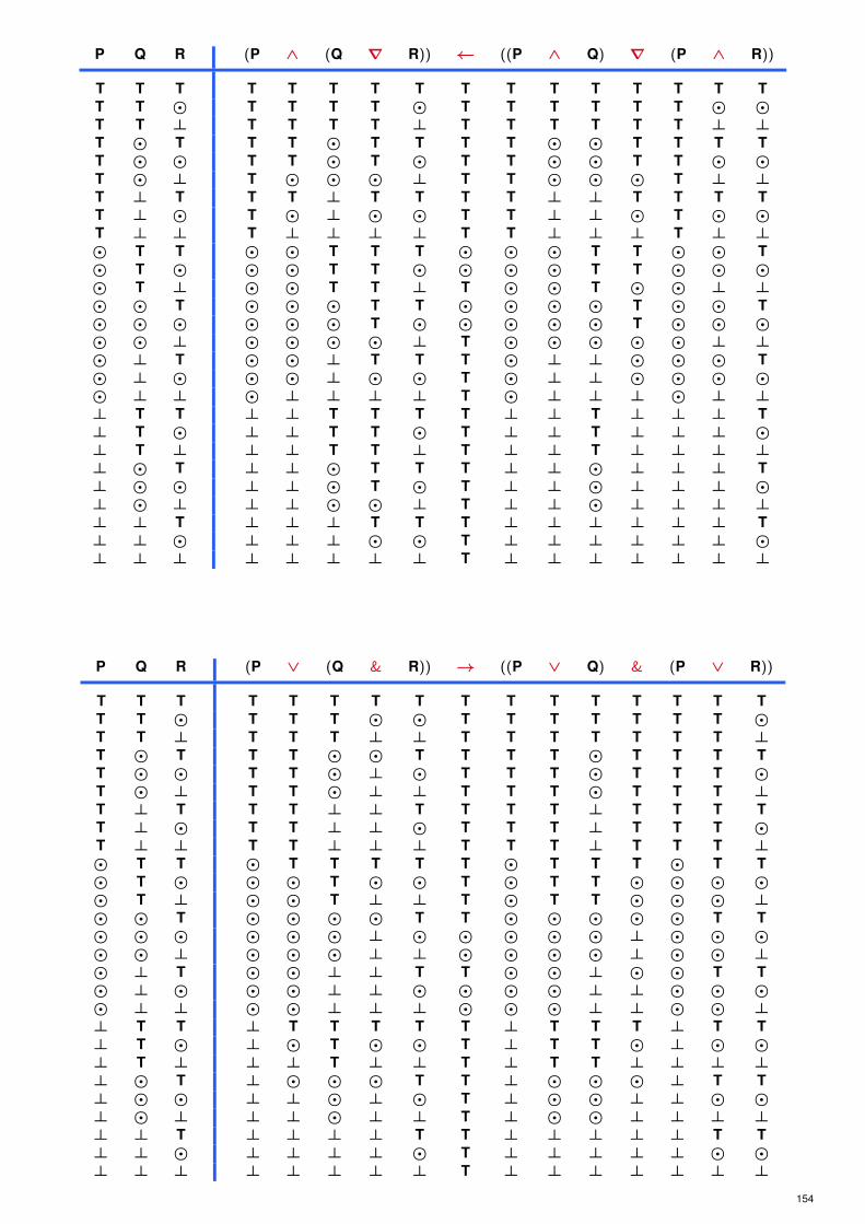
P Q R (P ∧ (Q ∇ R)) ← ((P ∧ Q) ∇ (P ∧ R))

T T T T T T T T T T T T T T T TT T � T T T T � T T T T T T � �T T ⊥ T T T T ⊥ T T T T T T ⊥ ⊥T � T T T � T T T T � � T T T TT � � T T � T � T T � � T T � �T � ⊥ T � � � ⊥ T T � � � T ⊥ ⊥T ⊥ T T T ⊥ T T T T ⊥ ⊥ T T T TT ⊥ � T � ⊥ � � T T ⊥ ⊥ � T � �T ⊥ ⊥ T ⊥ ⊥ ⊥ ⊥ T T ⊥ ⊥ ⊥ T ⊥ ⊥� T T � � T T T � � � T T � � T� T � � � T T � � � � T T � � �� T ⊥ � � T T ⊥ T � � T � � ⊥ ⊥� � T � � � T T � � � � T � � T� � � � � � T � � � � � T � � �� ⊥ � � � � ⊥ T � � � � � ⊥ ⊥� ⊥ T � � ⊥ T T T � ⊥ ⊥ � � � T� ⊥ � � � ⊥ � � T � ⊥ ⊥ � � � �� ⊥ ⊥ � ⊥ ⊥ ⊥ ⊥ T � ⊥ ⊥ ⊥ � ⊥ ⊥⊥ T T ⊥ ⊥ T T T T ⊥ ⊥ T ⊥ ⊥ ⊥ T⊥ T � ⊥ ⊥ T T � T ⊥ ⊥ T ⊥ ⊥ ⊥ �⊥ T ⊥ ⊥ ⊥ T T ⊥ T ⊥ ⊥ T ⊥ ⊥ ⊥ ⊥⊥ � T ⊥ ⊥ � T T T ⊥ ⊥ � ⊥ ⊥ ⊥ T⊥ � � ⊥ ⊥ � T � T ⊥ ⊥ � ⊥ ⊥ ⊥ �⊥ � ⊥ ⊥ ⊥ � � ⊥ T ⊥ ⊥ � ⊥ ⊥ ⊥ ⊥⊥ ⊥ T ⊥ ⊥ ⊥ T T T ⊥ ⊥ ⊥ ⊥ ⊥ ⊥ T⊥ ⊥ � ⊥ ⊥ ⊥ � � T ⊥ ⊥ ⊥ ⊥ ⊥ ⊥ �⊥ ⊥ ⊥ ⊥ ⊥ ⊥ ⊥ ⊥ T ⊥ ⊥ ⊥ ⊥ ⊥ ⊥ ⊥

P Q R (P ∨ (Q & R)) → ((P ∨ Q) & (P ∨ R))

T T T T T T T T T T T T T T T TT T � T T T � � T T T T T T T �T T ⊥ T T T ⊥ ⊥ T T T T T T T ⊥T � T T T � � T T T T � T T T TT � � T T � ⊥ � T T T � T T T �T � ⊥ T T � ⊥ ⊥ T T T � T T T ⊥T ⊥ T T T ⊥ ⊥ T T T T ⊥ T T T TT ⊥ � T T ⊥ ⊥ � T T T ⊥ T T T �T ⊥ ⊥ T T ⊥ ⊥ ⊥ T T T ⊥ T T T ⊥� T T � T T T T T � T T T � T T� T � � � T � � T � T T � � � �� T ⊥ � � T ⊥ ⊥ T � T T � � � ⊥� � T � � � � T T � � � � � T T� � � � � � ⊥ � � � � � ⊥ � � �� ⊥ � � � ⊥ ⊥ � � � � ⊥ � � ⊥� ⊥ T � � ⊥ ⊥ T T � � ⊥ � � T T� ⊥ � � � ⊥ ⊥ � � � � ⊥ ⊥ � � �� ⊥ ⊥ � � ⊥ ⊥ ⊥ � � � ⊥ ⊥ � � ⊥⊥ T T ⊥ T T T T T ⊥ T T T ⊥ T T⊥ T � ⊥ � T � � T ⊥ T T � ⊥ � �⊥ T ⊥ ⊥ ⊥ T ⊥ ⊥ T ⊥ T T ⊥ ⊥ ⊥ ⊥⊥ � T ⊥ � � � T T ⊥ � � � ⊥ T T⊥ � � ⊥ ⊥ � ⊥ � T ⊥ � � ⊥ ⊥ � �⊥ � ⊥ ⊥ ⊥ � ⊥ ⊥ T ⊥ � � ⊥ ⊥ ⊥ ⊥⊥ ⊥ T ⊥ ⊥ ⊥ ⊥ T T ⊥ ⊥ ⊥ ⊥ ⊥ T T⊥ ⊥ � ⊥ ⊥ ⊥ ⊥ � T ⊥ ⊥ ⊥ ⊥ ⊥ � �⊥ ⊥ ⊥ ⊥ ⊥ ⊥ ⊥ ⊥ T ⊥ ⊥ ⊥ ⊥ ⊥ ⊥ ⊥

154

Q P R ((P → Q) ∧ (Q → R)) → (P → R)

T T T T T T T T T T T T T TT T � T T T � T � � T T � �T T ⊥ T T T ⊥ T ⊥ ⊥ T T ⊥ ⊥T � T � T T T T T T T � T TT � � � T T � T � � T � T �T � ⊥ � T T ⊥ T ⊥ ⊥ T � � ⊥T ⊥ T ⊥ T T T T T T T ⊥ T TT ⊥ � ⊥ T T � T � � T ⊥ T �T ⊥ ⊥ ⊥ T T ⊥ T ⊥ ⊥ T ⊥ T ⊥� T T T � � � � T T T T T T� T � T � � � � T � T T � �� T ⊥ T � � � � � ⊥ � T ⊥ ⊥� � T � T � T � T T T � T T� � � � T � T � T � T � T �� ⊥ � T � � � � ⊥ T � � ⊥� ⊥ T ⊥ T � T � T T T ⊥ T T� ⊥ � ⊥ T � T � T � T ⊥ T �� ⊥ ⊥ ⊥ T � � � � ⊥ T ⊥ T ⊥⊥ T T T ⊥ ⊥ ⊥ ⊥ T T T T T T⊥ T � T ⊥ ⊥ ⊥ ⊥ T � T T � �⊥ T ⊥ T ⊥ ⊥ ⊥ ⊥ T ⊥ T T ⊥ ⊥⊥ � T � � ⊥ � ⊥ T T T � T T⊥ � � � � ⊥ � ⊥ T � T � T �⊥ � ⊥ � � ⊥ � ⊥ T ⊥ T � � ⊥⊥ ⊥ T ⊥ T ⊥ T ⊥ T T T ⊥ T T⊥ ⊥ � ⊥ T ⊥ T ⊥ T � T ⊥ T �⊥ ⊥ ⊥ ⊥ T ⊥ T ⊥ T ⊥ T ⊥ T ⊥

T-NORM AND T-CONORM

Remark 2.29Question When shall we speak of a conjunction or disjunction?

Like the weak connectives, the bold connectives meet the following minimal requirementsthat have been proposed in general for a conjunction resp. disjunction connective ◦ :

(1) Conjunction and disjunction are both associative:P ◦ (Q ◦ R) is equivalent to (P ◦ Q) ◦ R

(2) Conjunction and disjunction are both commutative: P ◦ Q is equivalent to Q ◦ P .

(3) Conjunction and disjunction are nondecreasing in both arguments:Using the ranking > > � > ⊥ for all interpretations I shall hold:

PI ≤ R ⇒ PI ◦? QI ≤ RI ◦? QI and PI ≤ RI ⇒ QI ◦? PI ≤ QI ◦? RI

(4) With ∧ a conjunction connective: If P is > , then P ∧ Q has the value of Q

(5) With ∨ a disjunction connective: If P is ⊥ , then P ∨ Q has the value of Q

Definition 2.30Given a linearly ordered set of truth values with > the greatest and ⊥ the least element.

A connective fulfilling the conditions on ∧ is called a t-norm anda connective fulfilling the conditions on ∨ is called a t-conorm .

156

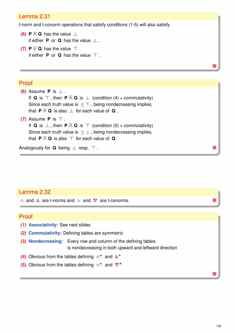
Lemma 2.31t-norm and t-conorm operations that satisfy conditions (1-5) will also satisfy

(6) P ∧ Q has the value ⊥if either P or Q has the value ⊥ .

(7) P ∨ Q has the value >if either P or Q has the value > .

Proof(6) Assume P is ⊥ .

If Q is > , then P ∧ Q is ⊥ (condition (4) + commutativity)Since each truth value is ≤ > , being nondecreasing implies,that P ∧ Q is also ⊥ for each value of Q .

(7) Assume P is > .If Q is ⊥ , then P ∧ Q is > (condition (5) + commutativity)Since each truth value is ≥ ⊥ , being nondecreasing implies,that P ∧ Q is also > for each value of Q .

Analogously for Q being ⊥ resp. > .

Lemma 2.32∧ and & are t-norms and ∨ and ∇ are t-conorms.

Proof(1) Associativity: See next slides

(2) Commutativity: Defining tables are symmetric

(3) Nondecreasing: Every row and column of the defining tablesis nondecreasing in both upward and leftward direction

(4) Obvious from the tables defining ∧? and &?

(5) Obvious from the tables defining ∨? and ∇?

158

P Q R (P ∧ (Q ∧ R)) ≡ ((P ∧ Q) ∧ R)

T T T T T T T T T T T T T TT T � T � T � � T T T T � �T T ⊥ T ⊥ T ⊥ ⊥ T T T T ⊥ ⊥T � T T � � � T T T � � � TT � � T � � � � T T � � � �T � ⊥ T ⊥ � ⊥ ⊥ T T � � ⊥ ⊥T ⊥ T T ⊥ ⊥ ⊥ T T T ⊥ ⊥ ⊥ TT ⊥ � T ⊥ ⊥ ⊥ � T T ⊥ ⊥ ⊥ �T ⊥ ⊥ T ⊥ ⊥ ⊥ ⊥ T T ⊥ ⊥ ⊥ ⊥� T T � � T T T T � � T � T� T � � � T � � T � � T � �� T ⊥ � ⊥ T ⊥ ⊥ T � � T ⊥ ⊥� � T � � � � T T � � � � T� � � � � � � � T � � � � �� ⊥ � ⊥ � ⊥ ⊥ T � � � ⊥ ⊥� ⊥ T � ⊥ ⊥ ⊥ T T � ⊥ ⊥ ⊥ T� ⊥ � � ⊥ ⊥ ⊥ � T � ⊥ ⊥ ⊥ �� ⊥ ⊥ � ⊥ ⊥ ⊥ ⊥ T � ⊥ ⊥ ⊥ ⊥⊥ T T ⊥ ⊥ T T T T ⊥ ⊥ T ⊥ T⊥ T � ⊥ ⊥ T � � T ⊥ ⊥ T ⊥ �⊥ T ⊥ ⊥ ⊥ T ⊥ ⊥ T ⊥ ⊥ T ⊥ ⊥⊥ � T ⊥ ⊥ � � T T ⊥ ⊥ � ⊥ T⊥ � � ⊥ ⊥ � � � T ⊥ ⊥ � ⊥ �⊥ � ⊥ ⊥ ⊥ � ⊥ ⊥ T ⊥ ⊥ � ⊥ ⊥⊥ ⊥ T ⊥ ⊥ ⊥ ⊥ T T ⊥ ⊥ ⊥ ⊥ T⊥ ⊥ � ⊥ ⊥ ⊥ ⊥ � T ⊥ ⊥ ⊥ ⊥ �⊥ ⊥ ⊥ ⊥ ⊥ ⊥ ⊥ ⊥ T ⊥ ⊥ ⊥ ⊥ ⊥

P Q R (P ∨ (Q ∨ R)) ≡ ((P ∨ Q) ∨ R)

T T T T T T T T T T T T T TT T � T T T T � T T T T T �T T ⊥ T T T T ⊥ T T T T T ⊥T � T T T � T T T T T � T TT � � T T � � � T T T � T �T � ⊥ T T � � ⊥ T T T � T ⊥T ⊥ T T T ⊥ T T T T T ⊥ T TT ⊥ � T T ⊥ � � T T T ⊥ T �T ⊥ ⊥ T T ⊥ ⊥ ⊥ T T T ⊥ T ⊥� T T � T T T T T � T T T T� T � � T T T � T � T T T �� T ⊥ � T T T ⊥ T � T T T ⊥� � T � T � T T T � � � T T� � � � � � � � T � � � � �� ⊥ � � � � ⊥ T � � � � ⊥� ⊥ T � T ⊥ T T T � � ⊥ T T� ⊥ � � � ⊥ � � T � � ⊥ � �� ⊥ ⊥ � � ⊥ ⊥ ⊥ T � � ⊥ � ⊥⊥ T T ⊥ T T T T T ⊥ T T T T⊥ T � ⊥ T T T � T ⊥ T T T �⊥ T ⊥ ⊥ T T T ⊥ T ⊥ T T T ⊥⊥ � T ⊥ T � T T T ⊥ � � T T⊥ � � ⊥ � � � � T ⊥ � � � �⊥ � ⊥ ⊥ � � � ⊥ T ⊥ � � � ⊥⊥ ⊥ T ⊥ T ⊥ T T T ⊥ ⊥ ⊥ T T⊥ ⊥ � ⊥ � ⊥ � � T ⊥ ⊥ ⊥ � �⊥ ⊥ ⊥ ⊥ ⊥ ⊥ ⊥ ⊥ T ⊥ ⊥ ⊥ ⊥ ⊥

P Q R (P & (Q & R)) ≡ ((P & Q) & R)

T T T T T T T T T T T T T TT T � T � T � � T T T T � �T T ⊥ T ⊥ T ⊥ ⊥ T T T T ⊥ ⊥T � T T � � � T T T � � � TT � � T ⊥ � ⊥ � T T � � ⊥ �T � ⊥ T ⊥ � ⊥ ⊥ T T � � ⊥ ⊥T ⊥ T T ⊥ ⊥ ⊥ T T T ⊥ ⊥ ⊥ TT ⊥ � T ⊥ ⊥ ⊥ � T T ⊥ ⊥ ⊥ �T ⊥ ⊥ T ⊥ ⊥ ⊥ ⊥ T T ⊥ ⊥ ⊥ ⊥� T T � � T T T T � � T � T� T � � ⊥ T � � T � � T ⊥ �� T ⊥ � ⊥ T ⊥ ⊥ T � � T ⊥ ⊥� � T � ⊥ � � T T � ⊥ � ⊥ T� � � � ⊥ � ⊥ � T � ⊥ � ⊥ �� ⊥ � ⊥ � ⊥ ⊥ T � ⊥ � ⊥ ⊥� ⊥ T � ⊥ ⊥ ⊥ T T � ⊥ ⊥ ⊥ T� ⊥ � � ⊥ ⊥ ⊥ � T � ⊥ ⊥ ⊥ �� ⊥ ⊥ � ⊥ ⊥ ⊥ ⊥ T � ⊥ ⊥ ⊥ ⊥⊥ T T ⊥ ⊥ T T T T ⊥ ⊥ T ⊥ T⊥ T � ⊥ ⊥ T � � T ⊥ ⊥ T ⊥ �⊥ T ⊥ ⊥ ⊥ T ⊥ ⊥ T ⊥ ⊥ T ⊥ ⊥⊥ � T ⊥ ⊥ � � T T ⊥ ⊥ � ⊥ T⊥ � � ⊥ ⊥ � ⊥ � T ⊥ ⊥ � ⊥ �⊥ � ⊥ ⊥ ⊥ � ⊥ ⊥ T ⊥ ⊥ � ⊥ ⊥⊥ ⊥ T ⊥ ⊥ ⊥ ⊥ T T ⊥ ⊥ ⊥ ⊥ T⊥ ⊥ � ⊥ ⊥ ⊥ ⊥ � T ⊥ ⊥ ⊥ ⊥ �⊥ ⊥ ⊥ ⊥ ⊥ ⊥ ⊥ ⊥ T ⊥ ⊥ ⊥ ⊥ ⊥

P Q R (P ∇ (Q ∇ R)) ≡ ((P ∇ Q) ∇ R)

T T T T T T T T T T T T T TT T � T T T T � T T T T T �T T ⊥ T T T T ⊥ T T T T T ⊥T � T T T � T T T T T � T TT � � T T � T � T T T � T �T � ⊥ T T � � ⊥ T T T � T ⊥T ⊥ T T T ⊥ T T T T T ⊥ T TT ⊥ � T T ⊥ � � T T T ⊥ T �T ⊥ ⊥ T T ⊥ ⊥ ⊥ T T T ⊥ T ⊥� T T � T T T T T � T T T T� T � � T T T � T � T T T �� T ⊥ � T T T ⊥ T � T T T ⊥� � T � T � T T T � T � T T� � � � T � T � T � T � T �� ⊥ � T � � ⊥ T � T � T ⊥� ⊥ T � T ⊥ T T T � � ⊥ T T� ⊥ � � T ⊥ � � T � � ⊥ T �� ⊥ ⊥ � � ⊥ ⊥ ⊥ T � � ⊥ � ⊥⊥ T T ⊥ T T T T T ⊥ T T T T⊥ T � ⊥ T T T � T ⊥ T T T �⊥ T ⊥ ⊥ T T T ⊥ T ⊥ T T T ⊥⊥ � T ⊥ T � T T T ⊥ � � T T⊥ � � ⊥ T � T � T ⊥ � � T �⊥ � ⊥ ⊥ � � � ⊥ T ⊥ � � � ⊥⊥ ⊥ T ⊥ T ⊥ T T T ⊥ ⊥ ⊥ T T⊥ ⊥ � ⊥ � ⊥ � � T ⊥ ⊥ ⊥ � �⊥ ⊥ ⊥ ⊥ ⊥ ⊥ ⊥ ⊥ T ⊥ ⊥ ⊥ ⊥ ⊥

160

Lemma 2.33Conditions (2-5) of Remark 2.29 uniquely determine classical conjunction and disjunction.

ProofCommutativity alone yields the following 8 symmetric tables

T

⊥

T

⊥

T ⊥

T T

T T

T ⊥⊥ T

T ⊥

T T

T ⊥

T ⊥⊥ ⊥

T ⊥

⊥ T

T T

⊥ ⊥⊥ T

T ⊥

⊥ T

T ⊥

⊥ ⊥⊥ ⊥

The red tables drop out for not being nondecreasing.(just to check rows and columns in leftward and upward direction)

The blue tables drop out for being neither a conjunction nor a disjunction(Condition (4) resp. (5) from Remark 2.29)

3. Non Truth Centered Semantical ConceptsQuasi-TautologiesQuasi-EntailmentExample: Logic of ParadoxDegree Entailment

COMPARISON OF LOGICS

I One way to evaluate different logical systems

is to compare their sets of tautologies and contradictions.

I Up to now all our semantical concepts

– tautology, contradiction, validity, entailment .... –

focussed on the truth value > .

The results were not so nice:

. KS3 and BI

3 have no tautologies.

. On the other hand, L3 does have tautologies.

I We will now look for alternatives.

DESIGNATED TRUTH VALUES

Remark 3.1With an m-valued logic it is customary

to distinguish a subset of the set Wm of truth values as designated.

Depending on the intended application of an m-valued logicthe designated truth-values include >and any other truth-values

that we wish to count as good or at least as not bad.

We can then define tautologies in terms of designated truth-values:

A formula is a relative tautology ⇐⇒it has a designated truth-value on every interpretation.

I If only the value > is designated,we end up with the definition of tautology (proper)

that we’ve been using up to now:A formula that always has the value > is a tautology.

I If both the values > and � are designated,we end up with so-called quasi-tautologies.

164


QUASI-TAUTOLOGY

Definition 3.2We will say that a formula F is a quasi-tautology ⇐⇒ F is never false.

Remark 3.3I Note that in classical logic the concepts of

being a tautology and being a quasi-tautology coincide,since a formula that is never false in classical logic is always true, and vice versa.

I But these two concepts do not coincide in 3-valued systems.

For example, although KS3 and BI

3 have no tautologies they both have quasi-tautologies:The formula A ∨¬A is a quasi-tautology in each of the two systems( A ∨¬A is also a quasi-tautology in L3 ).

A A ∨ ¬ A

T T T ⊥ T

� � � � �⊥ ⊥ T T ⊥

A A ∨BI ¬BI A

T T T ⊥ T

� � � � �⊥ ⊥ T T ⊥

166

Remark 3.4

Why might we be interested in quasi-tautologies?

I For one thing, we might be interested in avoiding falsehood

as much as we are interested in embracing truth.

If the former is the case, the set of quasi-tautologies should be of interest.

I The concept of a quasi-tautologyis a second way of generalizing the classical notion of a tautology

– as a formula that is never falserather than

as a formula that is always true –

and the concept therefore also has purely theoretical interest.

If we believe that the simple classical tautologies A→ A and A↔ Ashould remain tautologies within a 3-valued system,that would be a reason for preferring L3 to KS

3 and BI3 .

But preferring quasi-tautologies over tautologies (proper) is an alternative.

A A →K A

T T T T

� � � �⊥ ⊥ T ⊥

A A →BI A

T T T T

� � � �⊥ ⊥ T ⊥

A A ↔K A

T T T T

� � � �⊥ ⊥ T ⊥

A A ↔BI A

T T T T

� � � �⊥ ⊥ T ⊥

Every classical tautology is a quasi-tautology in both KS3 and BI

3 , and vice versa.(proofs below)

168

Lemma 3.5

The set of BI3 quasi-tautologies is exactly the set of classical tautologies.

Proof=⇒ Let F be a BI

3 quasi-tautology.Then F does not have the value ⊥ on any truth-value assignment,

and therefore, F does not have the value ⊥ on any classical interpretation.Since BI

3 is normal, it follows from the Normality Lemma 1.40,that F can only have the value > on any classical interpretation,

and consequently, F is a tautology of classical logic.

⇐= Conversely, assume that a formula F is not a BI3 quasi-tautology.

Then F has the value ⊥ on some truth-value assignment in BI3 .

This truth-value assignment must be a classical assignment,since the value � is contagious in BI

3 .It follows from the Normality Lemma

that F has the value ⊥ on this assignment in classical logic,and therefore F is not a classical tautology.

Lemma 3.6

The set of KS3 quasi-tautologies is exactly the set of classical tautologies.

ProofThe proof that every KS

3 quasi-tautology is a classical tautologyfollows again from the Normality Lemma 1.40.

The converse claim,that a formula F that is not a KS

3 quasi-tautology is also not a classical tautology,is equivalent to saying that

a formula F that has the value ⊥ on some truth-value assignment in KS3

will also have the value ⊥ on some classical assignment.

The restated claim holds triviallyif the assignment on which F has the value ⊥ in KS

3 is a classical assignment.• • •

170

• • •

So we need to establish thatif a formula F has the value ⊥ on some non classical truth-value assignment in KS

3 ,F will also have the value ⊥ on some classical assignment in KS

3 .

In order for F to have the value ⊥ in KS3 on an assignment

on which one or more of its atomic components have the value � ,uniformity must have kicked in at some point to override the � s

in favor of classical truth-values.And at each point where uniformity kicked in,

the same classical value would have resulted if the � had been a > or an ⊥ instead.(Compare the definitions of the truth functions!)

So if we replace all of the � s that the 3-valued assignment assignswith either > s or ⊥ s (it doesn’t matter which),

F will end up having the same value on the resulting classical assignmentas it did on the 3-valued assignment.

Lemma 3.7

Every L3 quasi-tautology is a classical tautology.

ProofThe proof that every L3 quasi-tautology is a classical tautologyfollows from the Normality Lemma 1.40:

If a formula is > or � on all interpretationsthen it can only be > on classical interpretations.

172

However, the other way round is problematic.

Lemma 3.8

1. Every classical tautologythat contains only negation, conjunction, and disjunction is an L3 quasi-tautology.

2. But some classical tautologiescontaining the conditional or the biconditional are not L3 quasi-tautologies.

Proof1. It follows from Lemma 3.6

that every classical tautology that contains only negation, conjunction, and disjunctionis an L3 tautologybecause negation, conjunction, and disjunction in L3 are defined the same as in KS

3 .

• • •

• • •

2. An example of a classical tautology containing a conditionalthat is not a quasi-tautology in L3 is ¬(A→¬A) ∨¬(¬A→ A) .

A ¬ (A → ¬ A) ∨ ¬ (¬ A → A)

T T T ⊥ ⊥ T T ⊥ ⊥ T T T

� ⊥ � T � � ⊥ ⊥ � � T �⊥ ⊥ ⊥ T T ⊥ T T T ⊥ ⊥ ⊥

An example of a classical tautology containing a biconditionalthat is not a quasi-tautology in L3 is ¬(A↔¬A) .

A ¬ (A ↔ ¬ A)

T T T ⊥ ⊥ T

� ⊥ � T � �⊥ T ⊥ ⊥ T ⊥

174

Lemma 3.9

The set of BE3 quasi-tautologies coincides with the set of classical tautologies.

ProofThe only formulas that are not tautologies in BE

3but might be quasi-tautologies are atomic formulas,for no other formulas can ever have the truth-value � in this system.

But these formulas are neither classical tautologies nor quasi-tautologies in BE3 ,

since they can have the value ⊥ .

So quasi-tautologies and tautologies coincide in BE3 ,

and we have already established that the BE3 tautologies

coincide with the set of classical tautologies. (Lemma 1.82)

SUMMARY ON QUASI-TAUTOLOGIES

I With KS3 , BI

3 and BE3

classical tautologies and quasi-tautologies coincide (Lemmata 3.5, 3.6, 3.9)

I With L3 every quasi-tautology is a classical tautology, (Lemma 3.7)

but not the other way round. (Lemma 3.8)

176

QUASI-CONTRADICTION

Definition 3.10A formula is a quasi-contradiction if it is never true;

that means that in a 3-valued system it always has the value ⊥ or the value � .

Lemma 3.11

The results concerning quasi-tautologies in the 3-valued systemsalso hold for quasi-contradictions:

1. In each of BI3 , BE

3 , and KS3 the set of quasi-contradictions coincides with the set of

classical contradictions.

2. Every L3 quasi-contradiction is a classical contradiction.

3. Some classical contradictions are not L3 quasi-contradictions.


QUASI-ENTAILMENT

Remark 3.12

I Originally, tautologies were considered the essence of a logic.(Or theorems in case of proof-theoretical approaches.)

I A more recent view is to consider logical consequence or entailment the central issue.Note: Tautologies can be derived from entailment as formulae which follow from nothing.

Definition 3.13

A set S of formulas quasi-entails a formula F , in symbols S |≈ F ⇐⇒there is no truth-value assignment on which

each of the formulas in S has the value > or �while F has the value ⊥ ;

that is, whenever each formula in has one of the values > or � , so does F .

An argument (S,F) is quasi-valid ⇐⇒ S quasi-entails F

Lemma 3.14

Every quasi-entailment in each of KS3 , L3 , BI

3 , and BE3 is a classical entailment.

ProofIf a set S of formulae quasi-entails a formula F in any of the four logics

then no interpretation maps all formulae of S to > or � , but maps F to ⊥ .

But then there is no classical interpretationon which all of the formulas in S have the value >

(none will have the value � on a classical interpretation)and F has the value ⊥ in that logic.

Since these logics are all normal,it follows from the Normality Lemma 1.40that that F has the value > on all classical interpretations,

which means that the entailment holds in classical logic.

180

Lemma 3.15

Not every classical entailment is a quasi-entailment in KS3 , L3 , BI

3 , and BE3 .

Proof

First Example: The classically valid argument F

F ∨ F

isn’t quasi-valid in BE3 .

When the premise F has the value � , the conclusion is ⊥ .

F F |≈ (F ∨BE F)

T T T T T T

� � ⊥ � ⊥ �⊥ ⊥ T ⊥ ⊥ ⊥

• • •

• • •

Second Example: The argument F ∧¬F

G

is valid in classical logic.

But it fails to be quasi-valid in any of KS3 , L3 , or BI

3 (although it is valid in all three logics).

F G (F ∧ ¬ F) |≈ G

T T T ⊥ ⊥ T T T

T � T ⊥ ⊥ T T �T ⊥ T ⊥ ⊥ T T ⊥� T � � � � T T

� � � � � � T �� ⊥ � � � � ⊥ ⊥⊥ T ⊥ ⊥ T ⊥ T T

⊥ � ⊥ ⊥ T ⊥ T �⊥ ⊥ ⊥ ⊥ T ⊥ T ⊥

F G (F ∧BI ¬BI F) |≈ G

T T T ⊥ ⊥ T T T

T � T ⊥ ⊥ T T �T ⊥ T ⊥ ⊥ T T ⊥� T � � � � T T

� � � � � � T �� ⊥ � � � � ⊥ ⊥⊥ T ⊥ ⊥ T ⊥ T T

⊥ � ⊥ ⊥ T ⊥ T �⊥ ⊥ ⊥ ⊥ T ⊥ T ⊥

Both tables are identical!

182

Remark 3.16Some classically valid arguments are also quasi-valid in more than one of the four systems.

The argument F ∧ G

F

is quasi-valid in KS3 , L3 , and BE

3 ,

and the argument F

F ∨ G

is quasi-valid in KS3 , L3 , and BI

3 .

F G F ∧ G |≈ F F ∧BE G |≈ F F |≈ F ∨ G F |≈ F ∨BI G

T T T T T T T T T T T T T T T T T T T T T TT � T � � T T T ⊥ � T T T T T T � T T T � �T ⊥ T ⊥ ⊥ T T T ⊥ ⊥ T T T T T T ⊥ T T T T ⊥� T � � T T � � ⊥ T T � � T � T T � T � � T� � � � � T � � ⊥ � T � � T � � � � T � � �� ⊥ � ⊥ ⊥ T � � ⊥ ⊥ T � � T � � ⊥ � T � � ⊥⊥ T ⊥ ⊥ T T ⊥ ⊥ ⊥ T T ⊥ ⊥ T ⊥ T T ⊥ T ⊥ T T⊥ � ⊥ ⊥ � T ⊥ ⊥ ⊥ � T ⊥ ⊥ T ⊥ � � ⊥ T ⊥ � �⊥ ⊥ ⊥ ⊥ ⊥ T ⊥ ⊥ ⊥ ⊥ T ⊥ ⊥ T ⊥ ⊥ ⊥ ⊥ T ⊥ ⊥ ⊥

SUMMARY ON QUASI ENTAILMENT

I Every quasi-entailment in each of KS3 , L3 , BI

3 , and BE3 is a classical entailment.

(Lemma 3.14)

I Not every classical entailment is a quasi-entailment in KS3 , L3 , BI

3 , and BE3 .

(Lemma 3.15)

184


LOGIC OF PARADOX

Graham Priest1948 –

LP : Logic of Paradox is formally given by

I Kleene’s Strong 3-Valued Logic KS3

I Quasi-Entailment

[Priest, 1979]

Dialetheism:� sentences are both > and ⊥

186

Valid quasi-entailments in KS3

A |≈ A ∨K B

A→K (B→K C) |≈ B→K (A→K C)

¬K A→K ¬K B |≈ B→K A

¬K¬K A |≈ A

A ∧K B |≈ A

¬K A |≈ A→K B

A,B |≈ A ∧K B

A |≈ B→K A

¬K(A ∨K B) |≈ ¬K A

¬K A |≈ ¬K(A ∧K B)

A,¬K B |≈ ¬K(A→K B)

A→K (A→K B) |≈ A→K B

A→K B |≈ ¬K B→K ¬K A

¬K A,¬K B |≈ ¬K(A ∨K B)

A |≈ ¬K¬K A

¬K(A→K B) |≈ A

A→K B |≈ (A ∧K C)→K (B ∧K C)

A→K ¬K A |≈ ¬K A

Apart from the ‘blue’ one all these are also valid entailments.

Not valid quasi-entailments in KS3 (but valid entailments in KS

3 )

A, ¬K A ∨K B |/≈ B Disjunctive Syllogism

A→K B, B→K C |/≈ A→K C Hypothetical Syllogism

A, A→K B |/≈ B Modus Ponens

A→K B, ¬K B |/≈ ¬K A Modus Tollens

A ∧K ¬K A |/≈ B Ex falso/contradictione quodlibet segitur

See truth tables and discussion on next slides.

Remark 3.17Using in truth tables a ∧ -formula instead of a (finite) set of formulae

I fits well for entailment (proper)

since F ∧ G is > ⇐⇒ both F and G are > .

I But it also fits well for quasi-entailment

since F ∧ G is > or � ⇐⇒ both F and G are either > or � .

188

DISJUNCTIVE SYLLOGISM

A B A ∧ (¬K A ∨K B) |≈ B

T T T T ⊥ T T T T T

T � T � ⊥ T � � T �T ⊥ T ⊥ ⊥ T ⊥ ⊥ T ⊥� T � � � � T T T T

� � � � � � � � T �� ⊥ � � � � � ⊥ ⊥ ⊥⊥ T ⊥ ⊥ T ⊥ T T T T

⊥ � ⊥ ⊥ T ⊥ T � T �⊥ ⊥ ⊥ ⊥ T ⊥ T ⊥ T ⊥

green row classical entailment

green, blue and red rows relevant cases for quasi-entailment

green and blue = correct; red = incorrect

Historical Example: Disjunctive Syllogism + Ex Falso Quodlibet Sequitur

Assumption: Sokrates exists and Sokrates doesn’t exist

1. ∧ -eliminationFrom Sokrates exists and Sokrates doesn’t existfollows Sokrates exists

2. ∧ -eliminationFrom Sokrates exists and Sokrates doesn’t existfollows Sokrates doesn’t exist

3. ∨ -introductionFrom Sokrates doesn’t existfollows Sokrates doesn’t exist or Men are Donkeys

4. disjunctive syllogismFrom Sokrates existsand Sokrates doesn’t exist or Men are Donkeysfollows Menschen are Donkeys

Conclusion: From something false everything follows

190

HYPOTHETICAL SYLLOGISMB A C (A →K B) ∧ (B →K C) |≈ A →K C

T T T T T T T T T T T T T TT T � T T T � T � � T T � �T T ⊥ T T T ⊥ T ⊥ ⊥ T T ⊥ ⊥T � T � T T T T T T T � T TT � � � T T � T � � T � � �T � ⊥ � T T ⊥ T ⊥ ⊥ T � � ⊥T ⊥ T ⊥ T T T T T T T ⊥ T TT ⊥ � ⊥ T T � T � � T ⊥ T �T ⊥ ⊥ ⊥ T T ⊥ T ⊥ ⊥ T ⊥ T ⊥� T T T � � � � T T T T T T� T � T � � � � � � T T � �� T ⊥ T � � � � � ⊥ ⊥ T ⊥ ⊥� � T � � � � � T T T � T T� � � � � � � � � � T � � �� ⊥ � � � � � � ⊥ T � � ⊥� ⊥ T ⊥ T � T � T T T ⊥ T T� ⊥ � ⊥ T � � � � � T ⊥ T �� ⊥ ⊥ ⊥ T � � � � ⊥ T ⊥ T ⊥⊥ T T T ⊥ ⊥ ⊥ ⊥ T T T T T T⊥ T � T ⊥ ⊥ ⊥ ⊥ T � T T � �⊥ T ⊥ T ⊥ ⊥ ⊥ ⊥ T ⊥ T T ⊥ ⊥⊥ � T � � ⊥ � ⊥ T T T � T T⊥ � � � � ⊥ � ⊥ T � T � � �⊥ � ⊥ � � ⊥ � ⊥ T ⊥ T � � ⊥⊥ ⊥ T ⊥ T ⊥ T ⊥ T T T ⊥ T T⊥ ⊥ � ⊥ T ⊥ T ⊥ T � T ⊥ T �⊥ ⊥ ⊥ ⊥ T ⊥ T ⊥ T ⊥ T ⊥ T ⊥

green row classical entailmentgreen, blue and red rows relevant cases for quasi-entailment


MODUS PONENS

A B A ∧ (A →K B) |≈ B

T T T T T T T T T

T � T � T � � T �T ⊥ T ⊥ T ⊥ ⊥ T ⊥� T � � � T T T T

� � � � � � � T �� ⊥ � � � � ⊥ ⊥ ⊥⊥ T ⊥ ⊥ ⊥ T T T T

⊥ � ⊥ ⊥ ⊥ T � T �⊥ ⊥ ⊥ ⊥ ⊥ T ⊥ T ⊥




192

MODUS TOLLENS

A B (A →K B) ∧ ¬K B |≈ ¬K A

T T T T T ⊥ ⊥ T T ⊥ T

T � T � � � � � ⊥ ⊥ T

T ⊥ T ⊥ ⊥ ⊥ T ⊥ T ⊥ T

� T � T T ⊥ ⊥ T T � �� T � �� ⊥ � � ⊥ � T ⊥ T � �⊥ T ⊥ T T ⊥ ⊥ T T T ⊥⊥ � ⊥ T � � � � T T ⊥⊥ ⊥ ⊥ T ⊥ T T ⊥ T T ⊥




EX FALSO/CONTRADICTIONE QUODLIBET SEGITUR

B is not quasi-entailed by A ∧K ¬K A (Paraconsistence)

A B A ∧K ¬K A |≈ B

T T T ⊥ ⊥ T T T

T � T ⊥ ⊥ T T �T ⊥ T ⊥ ⊥ T T ⊥� T � � � � T T

� � � � � � T �� ⊥ � � � � ⊥ ⊥⊥ T ⊥ ⊥ T ⊥ T T

⊥ � ⊥ ⊥ T ⊥ T �⊥ ⊥ ⊥ ⊥ T ⊥ T ⊥

There are no classical relevant cases

blue and red rows relevant cases for quasi-entailment

blue = correct; red = incorrect

194

Lemma 3.18

If two formulas F and G of KS3

have no propositional variables in common andif G is no quasi-tautology

then F |/≈ G holds.

ProofIf G is no quasi-tautology, then exists an interpretation I such that GI = ⊥ .Let J be like I except that for all the propositional variables A occurring in F : AJ = � .

It now follows that

I FJ = � : See Proof of Lemma 1.38

I GJ = ⊥ :

Since for all variables A occurring in G holds AJ = AI ,and consequently, GJ = GI = ⊥ .

Hence the assertion F |/≈ G .

RELATION TO RELEVANCE LOGIC

Lemma 3.18 shows that the Logic of Paradox is a kind of Relevance Logic:

But we still have the quasi-tautology F→K (G→K F)

F G F →K (G →K F)

T T T T T T T

T � T T � T T

T ⊥ T T ⊥ T T

� T � � T � �� ⊥ � T ⊥ T �⊥ T ⊥ T T ⊥ ⊥⊥ � ⊥ T � � ⊥⊥ ⊥ ⊥ T ⊥ T ⊥

196

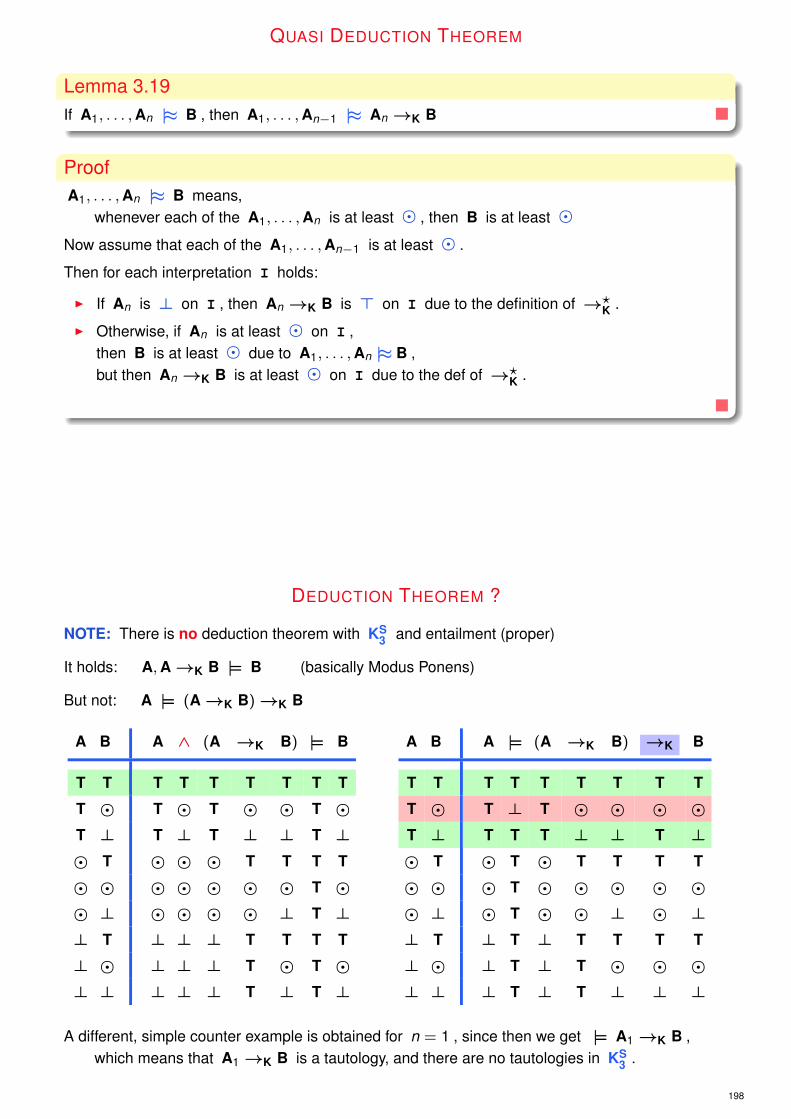
QUASI DEDUCTION THEOREM

Lemma 3.19If A1, . . . ,An |≈ B , then A1, . . . ,An−1 |≈ An →K B

ProofA1, . . . ,An |≈ B means,

whenever each of the A1, . . . ,An is at least � , then B is at least �

Now assume that each of the A1, . . . ,An−1 is at least � .

Then for each interpretation I holds:

I If An is ⊥ on I , then An →K B is > on I due to the definition of →?K .

I Otherwise, if An is at least � on I ,then B is at least � due to A1, . . . ,An |≈ B ,but then An →K B is at least � on I due to the def of →?

K .

DEDUCTION THEOREM ?

NOTE: There is no deduction theorem with KS3 and entailment (proper)

It holds: A,A→K B |= B (basically Modus Ponens)

But not: A |= (A→K B)→K B

A B A ∧ (A →K B) |= B

T T T T T T T T T

T � T � T � � T �T ⊥ T ⊥ T ⊥ ⊥ T ⊥� T � � � T T T T

� � � � � � � T �� ⊥ � � � � ⊥ T ⊥⊥ T ⊥ ⊥ ⊥ T T T T

⊥ � ⊥ ⊥ ⊥ T � T �⊥ ⊥ ⊥ ⊥ ⊥ T ⊥ T ⊥

A B A |= (A →K B) →K B

T T T T T T T T T

T � T ⊥ T � � � �T ⊥ T T T ⊥ ⊥ T ⊥� T � T � T T T T

� � � T � � � � �� ⊥ � T � � ⊥ � ⊥⊥ T ⊥ T ⊥ T T T T

⊥ � ⊥ T ⊥ T � � �⊥ ⊥ ⊥ T ⊥ T ⊥ ⊥ ⊥

A different, simple counter example is obtained for n = 1 , since then we get |= A1→K B ,which means that A1→K B is a tautology, and there are no tautologies in KS

3 .

198

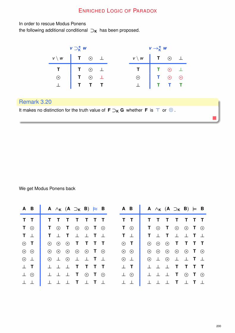
ENRICHED LOGIC OF PARADOX

In order to rescue Modus Ponensthe following additional conditional ⊃K has been proposed.

v ⊃?K w

v \ w T � ⊥

T T � ⊥� T � ⊥⊥ T T T

v →?K w

v \ w T � ⊥

T T � ⊥� T � �⊥ T T T

Remark 3.20It makes no distinction for the truth value of F ⊃K G whether F is > or � .

We get Modus Ponens back

A B A ∧K (A ⊃K B) |≈ B

T T T T T T T T T

T � T � T � � T �T ⊥ T ⊥ T ⊥ ⊥ T ⊥� T � � � T T T T

� � � � � � � T �� ⊥ � ⊥ � ⊥ ⊥ T ⊥⊥ T ⊥ ⊥ ⊥ T T T T

⊥ � ⊥ ⊥ ⊥ T � T �⊥ ⊥ ⊥ ⊥ ⊥ T ⊥ T ⊥

A B A ∧K (A ⊃K B) |= B

T T T T T T T T T

T � T � T � � T �T ⊥ T ⊥ T ⊥ ⊥ T ⊥� T � � � T T T T

� � � � � � � T �� ⊥ � ⊥ � ⊥ ⊥ T ⊥⊥ T ⊥ ⊥ ⊥ T T T T

⊥ � ⊥ ⊥ ⊥ T � T �⊥ ⊥ ⊥ ⊥ ⊥ T ⊥ T ⊥

200

‘ENRICHED’ QUASI DEDUCTION THEOREM

Lemma 3.21If A1, . . . ,An |≈ B , then A1, . . . ,An−1 |≈ An ⊃K B

ProofA1, . . . ,An |≈ B means,

whenever each of the A1, . . . ,An is at least � , then B is at least �

Now assume that each of the A1, . . . ,An−1 is at least � .

Then for each interpretation I holds:

I If An is ⊥ on I , then An ⊃K B is > on I due to the definition of ⊃?K .

I Otherwise, if An is at least � on I ,then B is at least � due to A1, . . . ,An |≈ B ,but then An ⊃K B is at least � on I due to the def of ⊃?

K .

HYPOTHETICAL SYLLOGISM

A B C ((A ⊃K B) ∧ (B ⊃K C)) |≈ (A ⊃K C)

T T T T T T T T T T T T T TT T � T T T � T � � T T � �T T ⊥ T T T ⊥ T ⊥ ⊥ T T ⊥ ⊥T � T T � � � � T T T T T TT � � T � � � � � � T T � �T � ⊥ T � � ⊥ � ⊥ ⊥ T T ⊥ ⊥T ⊥ T T ⊥ ⊥ ⊥ ⊥ T T T T T TT ⊥ � T ⊥ ⊥ ⊥ ⊥ T � T T � �T ⊥ ⊥ T ⊥ ⊥ ⊥ ⊥ T ⊥ T T ⊥ ⊥� T T � T T T T T T T � T T� T � � T T � T � � T � � �� T ⊥ � T T ⊥ T ⊥ ⊥ T � ⊥ ⊥� � T � � � � � T T T � T T� � � � � � � � � � T � � �� ⊥ � � � ⊥ � ⊥ ⊥ T � ⊥ ⊥� ⊥ T � ⊥ ⊥ ⊥ ⊥ T T T � T T� ⊥ � � ⊥ ⊥ ⊥ ⊥ T � T � � �� ⊥ ⊥ � ⊥ ⊥ ⊥ ⊥ T ⊥ T � ⊥ ⊥⊥ T T ⊥ T T T T T T T ⊥ T T⊥ T � ⊥ T T � T � � T ⊥ T �⊥ T ⊥ ⊥ T T ⊥ T ⊥ ⊥ T ⊥ T ⊥⊥ � T ⊥ T � T � T T T ⊥ T T⊥ � � ⊥ T � � � � � T ⊥ T �⊥ � ⊥ ⊥ T � ⊥ � ⊥ ⊥ T ⊥ T ⊥⊥ ⊥ T ⊥ T ⊥ T ⊥ T T T ⊥ T T⊥ ⊥ � ⊥ T ⊥ T ⊥ T � T ⊥ T �⊥ ⊥ ⊥ ⊥ T ⊥ T ⊥ T ⊥ T ⊥ T ⊥

202

MODUS TOLLENS

A B ((A ⊃K B) ∧ ¬K B) |≈ ¬K A

T T T T T ⊥ ⊥ T T ⊥ T

T � T � � � � � ⊥ ⊥ T

T ⊥ T ⊥ ⊥ ⊥ T ⊥ T ⊥ T

� T � T T ⊥ ⊥ T T � �� T � �� ⊥ � ⊥ ⊥ ⊥ T ⊥ T � �⊥ T ⊥ T T ⊥ ⊥ T T T ⊥⊥ � ⊥ T � � � � T T ⊥⊥ ⊥ ⊥ T ⊥ T T ⊥ T T ⊥

green row classical entailmentgreen, blue and red rows relevant cases for quasi-entailment


Same problem as with →K !


DEGREE ENTAILMENT

Up to now we had two concepts of entailment:

1. preserving truth (as in entailment (proper) based on > )

2. preserving non-falsehood (as in quasi-entailment)

We will now introduce a third concept of entailment (degree-entailment).

Definition 3.22We rank the three truth-values as > > � > ⊥ .

I We will say that a set S of formulas degree-entails a formula F , in symbols S |≤ F⇐⇒F ’s value can never be less than the least value of the formulas in S .

I An argument is degree-valid in a 3-valued system ⇐⇒the set of its premises degree-entails its conclusion.

Lemma 3.23

Every degree-entailmentof a formula F by a set S of formulaethat holds in BI

3 , BE3 , KS

3 , or L3

is a classical entailment.

ProofIn case of all formulae in S are true, the degree-entailment requires F to be true as well,i.e. we have classical entailment.

206

Lemma 3.24

Degree-entailment is equivalent to entailment proper plus quasi-entailment.

ProofGiven an argument (S,F) .

=⇒ Assume S |≤ F .

If all formulae in S are > , then also F must be > . Hence: S |= F

If all formulae in S are at least � , then also F must be at least � . Hence: S |≈ F

⇐= Assume S |= F and S |≈ F

If all formulae in S are at least � , then S |≈ F implies that also F is at least � .

If all formulae in S are at least > , then S |= F implies that also F is at least > .

Consequently: S |≤ F .

Lemma 3.25

Not every classical entailment is a degree-entailment in KS3 ,

and ditto for the other three systems L3 , BI3 , and BE

3 .

ProofFrom Lemma 3.15 we know,

that not every classical entailment is a quasi-entailment in KS3 , L3 , BI

3 , and BE3 .

But due to the preceding Lemma 3.24being a degree entailment would imply being a quasi-entailment.

208

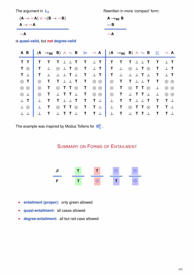
The argument in L3

(A→¬A) ∨ ¬(B→¬B)

A→¬A

¬A

is quasi-valid, but not degree-valid

Rewritten in more ‘compact’ form:

A→BE B

∼B

¬A

A B (A →BE B) ∧ ∼ B |≈ ¬ A (A →BE B) ∧ ∼ B |≤ ¬ A

T T T T T ⊥ ⊥ T T ⊥ T T T T ⊥ ⊥ T T ⊥ T

T � T ⊥ � ⊥ T � T ⊥ T T ⊥ � ⊥ T � T ⊥ T

T ⊥ T ⊥ ⊥ ⊥ T ⊥ T ⊥ T T ⊥ ⊥ ⊥ T ⊥ T ⊥ T

� T � T T ⊥ ⊥ T T � � � T T ⊥ ⊥ T T � �� T � T T � T � � � T � T T � ⊥ � �� ⊥ � T ⊥ T T ⊥ T � � � T ⊥ T T ⊥ ⊥ � �⊥ T ⊥ T T ⊥ ⊥ T T T ⊥ ⊥ T T ⊥ ⊥ T T T ⊥⊥ � ⊥ T � T T � T T ⊥ ⊥ T � T T � T T ⊥⊥ ⊥ ⊥ T ⊥ T T ⊥ T T ⊥ ⊥ T ⊥ T T ⊥ T T ⊥

The example was inspired by Modus Tollens for BE3 .

SUMMARY ON FORMS OF ENTAILMENT

S

F

T

T

T

�

�

T

�

�

I entailment (proper): only green allowed

I quasi-entailment: all cases allowed

I degree-entailment: all but red case allowed

210

4. Derivation Systems for 3-Valued Propositional LogicPrelude: A Derivation System for Classical Propositional LogicAn Axiomatic System for Łukasiewicz’s 3-Valued LogicCompleteness of 3-valued Łukasiewicz’s LogicApplication: Independence of AxiomsA Pavelka-Style Derivation System for Łukasiewicz Logic


FIRST APPROACH

General Idea: We need axioms and rules

I Axioms : A certain set of formulas

The Axioms are good formulae, e.g., formulae which shall be true

I Rules of Inference and/or Rules of Proof:

A, ...,B/C where A , . . . , B and C are formulas

I If our axioms are formulae we need a Rule of Substitution

Disadvantages:

. Axioms and an explicit substitution inference rule make derivations longer!

. Correct rules of substitution and their correct application may be tricky

SECOND APPROACH

Definition 4.1

I An axiom schema stands for infinitely many axioms,namely, all formulas that have the overall form exemplified by the schema.

I We define an instance of an axiom schema to be any formula that results from uniformsubstitution of formulas of the language (not necessarily distinct) for each of the lettersoccurring on the axiom schema.

I By uniform substitution we mean that in a given instance, the same formula must besubstituted for every occurrence of the same letter.

We write: F // P for the uniform substitution of P by F .

Suggested reading: F instead of P .

214

AXIOMATIC SYSTEM FOR CLASSICAL PROPOSITIONAL LOGIC

Definition 4.2

CLA (Classical propositional Logic Axiomatic system)

I Axiom Schemata

CL1 P→ (Q→ P)

CL2 (P→ (Q→ R))→ ((P→ Q)→ (P→ R))

CL3 (¬P→¬Q)→ (Q→ P)

I Rule of InferenceMP (Modus Ponens) From P and P→ Q , infer Q .

Remark 4.3Other Names for MP: separation, implication elimination or detachment rule(MP is often stated as rule of proof)

Remark 4.4I Each of the axiom schemata is has the form of a tautology with P , Q and R understood as

propositional variables. Truth-table for CL2 :

P Q R (P → (Q → R)) → ((P → Q) → (P → R))

T T T T T T T T T T T T T T T T

T T ⊥ T ⊥ T ⊥ ⊥ T T T T ⊥ T ⊥ ⊥T ⊥ T T T ⊥ T T T T ⊥ ⊥ T T T T

T ⊥ ⊥ T T ⊥ T ⊥ T T ⊥ ⊥ T T ⊥ ⊥⊥ T T ⊥ T T T T T ⊥ T T T ⊥ T T

⊥ T ⊥ ⊥ T T ⊥ ⊥ T ⊥ T T T ⊥ T ⊥⊥ ⊥ T ⊥ T ⊥ T T T ⊥ T ⊥ T ⊥ T T

⊥ ⊥ ⊥ ⊥ T ⊥ T ⊥ T ⊥ T ⊥ T ⊥ T ⊥

That CL1 and CL3 are tautologies can be verified analogously.

I The instances of CL1− 3 are also tautologies (proof by induction)

I Modus Ponens is a truth-preserving rule:If P and P→ Q are both true, then Q must be true as well.

216

DERIVATIONS

Definition 4.5

A derivation is a finite sequence of formulas each of which is

1. designated as an assumption, or

2. is an instance of an axiom schema, or

3. can be derived from earlier formulas in the sequence using the derivation rule MP.

ConventionIn addition, the formulas designated as assumptions must begin the derivation.

If a formula F is the last formula in a derivationthen we speak of a derivation of F .

Definition 4.6

I A formula F of L3 is derivable from a set S of formulas – S ` F , for short – ⇐⇒there is a derivation of F such that all assumptions are elements of S .

I A formula F is provable – ` F , for short – ⇐⇒ F is derivable from the empty set.

Example 4.7

Here is an example of a derivation annotated in a standard way:

1 F Assumption

2 (G→ F)→ (F→ H) Assumption

3 F→ (G→ F) CL1 F//P, G//Q

4 G→ F 1,3 MP

5 F→ H 2,4 MP

6 H 1,5 MP

Example 4.8

The following derivation shows that A→ B is derivable from ¬A :

1 ¬A Assumption

2 ¬A→ (¬B→¬A) CL1 ¬A//P, ¬B//Q

3 ¬B→¬A 1,2 MP

4 (¬B→¬A)→ (A→ B) CL3 B//P, A//Q

5 A→ B 3,4 MP

218

Lemma 4.9

For a deductive system consisting of axiom schemas and MP holds:

(a) If S ` A , then S′ ` A for every superset S′ of S .

(b) Hence, in particular, if ` A , then S ` A for every set S of formulas

(c) Hence, in particular, if A is an axiom, then S ` A for every set S of formulas

(d) If S ` A , then there is a finite subset S′ of S such that S′ ` A .

(e) If A belongs to S , then S ` A .

(f) If S ` A and S ` A→ B , then S ` B

ProofRather trivial from Definition 4.5 (derivation) and Definition 4.6 (derivabilty).

For point 6 we have to ‘concatenate’ the derivations of A and of A→ B ,resort to get the assumptions at the beginning,and then to apply the rule of inference MP.

Definition 4.10

I A derivation that does not contain any assumptions is called a proof.

I A formula F is called a theorem if there is a proof ending with formula F .

We may call this proof a proof of the theorem F .

Example 4.11

1 A→ ((A→ A)→ A) CL1 A//P, A→ A//Q

2 (A→ ((A→ A)→ A))→ CL2 A//P, A→ A//Q, A//R

((A→ (A→ A))→ (A→ A))

3 (A→ (A→ A))→ (A→ A) 1,2 MP

4 A→ (A→ A) CL1 A//P, A//Q

5 A→ A 3,4 MP

The proof just given establishes that A→ A is a theorem.

220

CONSISTENCY

Definition 4.12

I A set S of formulas is (syntactically) consistent ⇐⇒there is no formula F such that both F and ¬F are provable from S .

I A set S of formulas is (syntactically) inconsistent ⇐⇒there exists a formula F such that both F and ¬F are provable from S .

I And S is maximally consistent ⇐⇒. S is syntactically consistent, and

. S ` F for any formula F such that S ∪ {F } is syntactically consistent.

Definition 4.13A set S of formulas is semantically consistent or satisfiable ⇐⇒

there is an interpretation on which all formulas in S evaluate to > .

SOUNDNESS

Definition 4.14A derivation system is said to be sound for classical propositional logic ⇐⇒(a) all theorems are tautologies and

(b) whenever a formula F is derivable from a set S of formulas,then F is also entailed by the set S .

Lemma 4.15The system CLA is sound.

ProofCLA is a sound derivation system,because all its axioms are tautologies and its single rule of inference is truth-preserving.(cf. Remark 4.4)

222

COMPLETENESS

Definition 4.16I A derivation system is said to be weakly complete for classical propositional logic ⇐⇒

every tautology of classical logic is a theorem in the system

I A derivation system is said to be strongly complete, or just complete ⇐⇒in addition whenever a set S of formulas entails a formula F , F is also derivable from Swithin the system

I A derivation system is adequate for classical propositional logic ⇐⇒it is both sound and complete.

CLA is complete as well as sound for classical propositional logic.

Theorem 4.17

For a formula A of CL and a set S of formulae of CL holds:

. If S |= A, then S ` A (Strong Completeness Theorem)

. If |= A, then ` A (Weak Completeness Theorem)

Question about CompletenessHow to derive a tautology like F ∨ (F→ G) in CLA ?

AnswerRewrite formulas containing ∧ , ∨ , and ↔ ,

to formulas that contain only ¬ and → .

Definition 4.18

P ∨ Q := ¬P→ Q

P ∧ Q := ¬(P→¬Q)

P↔ Q := (P→ Q) ∧ (Q→ P), which turns into ¬((P→ Q)→¬(Q→ P))

Example 4.19

To show that F ∨ (F→ G) is a theoremwe first convert the formula to ¬F→ (F→ G) using the preceding definition for disjunction,then we construct a derivation for the latter formula. (see next slides)

224

1 ((¬F→ ((¬G→¬F)→ (F→ G)))→ CL1 (¬F→ ((¬G→¬F)→((¬F→ (¬G→¬F))→ (¬F→ (F→ G))))→ (F→ G)))→

(((¬G→¬F)→ (F→ G))→ ((¬F→ (¬G→¬F))→((¬F→ ((¬G→¬F)→ (F→ G)))→ (¬F→ (F→ G))//P

((¬F→ (¬G→¬F))→ (¬G→¬F)→ (F→ G)//Q(¬F→ (F→ G)))))

2 (¬F→ ((¬G→¬F)→ (F→ G))→ CL2 ¬F//P, ¬G→¬F//Q((¬F→ (¬G→¬F))→ (¬F→ (F→ G))) F→ G//R

3 ((¬G→¬F)→ (F→ G))→ 1,2 MP((¬F→ ((¬G→¬F)→ (F→ G)))→

((¬F→ (¬G→¬F))→ (¬F→ (F→ G))))

4 (((¬G→¬F)→ (F→ G))→ CL2 (¬G→¬F)→ (F→ G)//P((¬F→ ((¬G→¬F)→ (F→ G)))→ ¬F→ ((¬G→¬F)→((¬F→ (¬G→¬F))→ (F→ G))//Q

(¬F→ (F→ G)))))→ (¬F→ (¬G→¬F))→((((¬G→¬F)→ (F→ G))→ (¬F→ (F→ G))//R(¬F→ ((¬G→¬F)→ (F→ G))))→

(((¬G→¬F)→ (F→ G))→((¬F→ (¬G→¬F))→

(¬F→ (F→ G)))))

5 (((¬G→¬F)→ (F→ G))→ 3,4 MP

(¬F→ ((¬G→¬F)→ (F→ G))))→(((¬G→¬F)→ (F→ G))→

((¬F→ (¬G→¬F))→(¬F→ (F→ G))))

6 ((¬G→¬F)→ (F→ G))→ CL1 ¬F//Q

(¬F→ ((¬G→¬F)→ (F→ G))) (¬G→¬F)→ (F→ G)//P

7 ((¬G→¬F)→ (F→ G))→ 5,6 MP

((¬F→ (¬G→¬F))→(¬F→ (F→ G)))

8 ¬F→ (¬G→¬F) CL1 ¬F//P, ¬G//Q

9 (¬G→¬F)→ (F→ G) CL3 G//P, F//Q

10 (¬F→ (¬G→¬F))→ (¬F→ (F→ G)) 9, 7 MP

11 ¬F→ (F→ G) 8, 10 MP

We may conclude that F ∨ (F→ G) is a theorem of CLA .

226

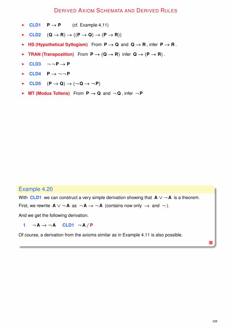
DERIVED AXIOM SCHEMATA AND DERIVED RULES

I CLD1 P→ P (cf. Example 4.11)

I CLD2 (Q→ R)→ ((P→ Q)→ (P→ R))

I HS (Hypothetical Syllogism) From P→ Q and Q→ R , infer P→ R .

I TRAN (Transposition) From P→ (Q→ R) infer Q→ (P→ R) .

I CLD3 ¬¬P→ P

I CLD4 P→¬¬P

I CLD5 (P→ Q)→ (¬Q→¬P)

I MT (Modus Tollens) From P→ Q and ¬Q , infer ¬P

Example 4.20With CLD1 we can construct a very simple derivation showing that A ∨ ¬A is a theorem.

First, we rewrite A ∨ ¬A as ¬A→¬A (contains now only → and ¬ ).

And we get the following derivation.

1 ¬A→¬A CLD1 ¬A//P

Of course, a derivation from the axioms similar as in Example 4.11 is also possible.

228

Remark 4.21Let’s reconsider the derivation of the theorem ¬F→ (F→ G) (resp. F ∨ (F→ G) )

Excluding the lines 8 and 9 of the derivation in Example 4.19the main purpose

is to derive ¬F→ (F→ G) (line 11)from ¬F→ (¬G→¬F) and (¬G→¬F)→ (F→ G) (lines 8 and 9).(Then line 11 is obtained with the help of line 7 + MP twice)

Examining these formulas we see that they are instances of a general inference patternthat derives a formula of the form P→ Rfrom formulas of the form P→ Q and Q→ R .

To introduce this inference pattern as a derived rule yields:

HS (Hypothetical Syllogism). From P→ Q and Q→ R , infer P→ R .

The justification of HS goes best via the derived axiom

CLD2 . (Q→ R)→ ((P→ Q)→ (P→ R))

This axiom is justified by the derivation on the next slide.Compare with the previous derivation of F ∨ (F→ G) in Example 4.19:We reproduce the first 7 lines.

CLD2 (Q→ R)→ ((P→ Q)→ (P→ R))

1 ((P→ (Q→ R))→ ((P→ Q)→ (P→ R)))→ CL1 (P→ (Q→ R))→((Q→ R)→ ((P→ Q)→ (P→ R))//P,

((P→ (Q→ R))→ ((P→ Q)→ (P→ R)))) Q→ R//Q

2 (P→ (Q→ R))→ ((P→ Q)→ (P→ R)) CL2 P//P, Q//Q, R//R

3 (Q→ R)→ 1,2 MP

((P→ (Q→ R))→ ((P→ Q)→ (P→ R)))

4 ((Q→ R)→ CL2 Q→ R//P,

((P→ (Q→ R))→ ((P→ Q)→ (P→ R))))→ P→ (Q→ R)//Q,

(((Q→ R)→ (P→ (Q→ R)))→ (P→ Q)→ (P→ R)//R

((Q→ R)→ ((P→ Q)→ (P→ R))))

5 ((Q→ R)→ (P→ (Q→ R)))→ 3,4 MP

((Q→ R)→ ((P→ Q)→ (P→ R)))

6 (Q→ R)→ (P→ (Q→ R)) CL1 Q→ R//P, P//Q

7 (Q→ R)→ ((P→ Q)→ (P→ R)) 5,6 MP

230


1 P→ Q Assumption

2 Q→ R Assumption

3 (Q→ R)→ ((P→ Q)→ (P→ R)) CLD2 P//P, Q//Q, R//R

4 (P→ Q)→ (P→ R) 2,3 MP

5 P→ R 1,4 MP

This derivation shows: If we already have P→ Q and Q→ R ,whether or not they are assumptions,we can derive P→ R .

Remark 4.22Using HS, we can seriously shorten the derivation of ¬F→ (F→ G) given in Example 4.19:

1 ¬F→ (¬G→¬F) CL1 ¬F//P, ¬G//Q (was 8)

2 (¬G→¬F)→ (F→ G) CL3 G//P, F//Q (was 9)

3 ¬F→ (F→ G) 1,2 HS

TRAN (Transposition). From P→ (Q→ R) infer Q→ (P→ R) .

1 P→ (Q→ R) Assumption

2 ((P→ Q)→ (P→ R))→ ((Q→ (P→ Q))→ CLD2 Q//P, P→ Q//Q,

(Q→ (P→ R))) P→ R//R

3 (((P→ Q)→ (P→ R))→ CL2 (P→ Q)→ (P→ R)//P,

((Q→ (P→ Q))→ (Q→ (P→ R))))→ Q→ (P→ Q)//Q,

(((P→ Q)→ (P→ R))→ (Q→ (P→ Q)))→ Q→ (P→ R)//R

(((P→ Q)→ (P→ R))→ (Q→ (P→ R)))

4 ((P→ Q)→ (P→ R))→ (Q→ (P→ Q))→ 2,3 MP

(((P→ Q)→ (P→ R))→ (Q→ (P→ R)))

5 Q→ (P→ Q) CL1 Q//P, P//Q

6 (Q→ (P→ Q))→ (((P→ Q)→ (P→ R))→ CL1 Q→ (P→ Q)//P,

(Q→ (P→ Q))) (P→ Q)→ (P→ R)//Q

7 ((P→ Q)→ (P→ R))→ (Q→ (P→ Q)) 5,6 MP

8 ((P→ Q)→ (P→ R))→ (Q→ (P→ R)) 4,7 MP

9 (P→ (Q→ R))→ ((P→ Q)→ (P→ R)) CL2 P//P, Q//Q, R//R

10 (P→ (Q→ R))→ (Q→ (P→ R)) 8,9 HS

11 Q→ (P→ R) 1,10 MP

232

CLD3 ¬¬P→ P

1 ¬¬P→ (¬¬¬¬P→¬¬P) CL1 ¬¬P//P, ¬¬¬¬P//Q

2 (¬¬¬¬P→¬¬P)→ (¬P→¬¬¬P) CL3 ¬¬¬P//P, ¬P//Q

3 ¬¬P→ (¬P→¬¬¬P) 1,2 HS

4 (¬P→¬¬¬P)→ (¬¬P→ P) CL3 P//P, ¬¬P//Q

5 ¬¬P→ (¬¬P→ P) 3,4 HS

6 (¬¬P→ (¬¬P→ P))→ CL2 ¬¬P//P, ¬¬P//Q, P//R

((¬¬P→¬¬P)→ (¬¬P→ P))

7 (¬¬P→¬¬P)→ (¬¬P→ P) 5,6 MP

8 ¬¬P→¬¬P CLD1 ¬¬P//P

9 ¬¬P→ P 7,8 MP

CLD4 P→¬¬P

1 ¬¬¬P→¬P CLD3 ¬P//P

2 (¬¬¬P→¬P)→ (P→¬¬P) CL3 ¬¬P//P, P//Q

3 P→¬¬P 1,2 MP

CLD5 (P→ Q)→ (¬Q→¬P) (Converse of CL3 ):

1 (Q→¬¬Q)→ ((P→ Q)→ (P→¬¬Q)) CLD2 P//P, Q//Q, ¬¬Q//R

2 Q→¬¬Q CLD4 Q//P

3 (P→ Q)→ (P→¬¬Q) 1,2 MP

4 (P→¬¬Q)→ ((¬¬P→ P)→ CLD2 ¬¬P//P, P//Q, ¬¬Q//R

(¬¬P→¬¬Q))

5 (¬¬P→ P)→ ((P→¬¬Q)→ 4 TRAN

(¬¬P→¬¬Q))

6 ¬¬P→ P CLD3 P//P

7 (P→¬¬Q)→ (¬¬P→¬¬Q) 5,6 MP

8 (P→ Q)→ (¬¬P→¬¬Q) 3,7 HS

9 (¬¬P→¬¬Q)→ (¬Q→¬P) CL3 ¬P//P, ¬Q//Q

10 (P→ Q)→ (¬Q→¬P) 8,9 HS

234

MODUS TOLLENS

MT (Modus Tollens). From P→ Q and ¬Q , infer ¬P

1 P→ Q Assumption

2 ¬Q Assumption

3 (P→ Q)→ (¬Q→¬P) CLD5 P//P, Q//Q

4 ¬Q→¬P 1,3 MP

5 ¬P 2,4 MP

Example 4.23

If the economy is sound, then the unemployment rate is low or spending is high.

If the unemployment rate is low, then most people are well off.

If spending is high, then most people are well off.

It’s not true that most people are well off.

The economy isn’t sound.

First we symbolize the argument: E→ (U ∨ S)

U→ W

S→ W

¬W

¬E

And we rewrite the first premise as E→ (¬U→ S) . (A derivation is on the next slide.)

236

1 E→ (¬U→ S) Assumption (rewritten from E→ (U ∨ S))

2 U→ W Assumption

3 S→ W Assumption

4 ¬W Assumption

5 ¬U 2,4 MT

6 ¬S 3,4 MT

7 (¬U→ S)→ (¬S→¬¬U) CLD5 ¬U//P, S//Q

8 ¬S→ ((¬U→ S)→¬¬U) 7 TRAN

9 (¬U→ S)→¬¬U 6,8 MP

10 ((¬U→ S)→¬¬U)→ CLD5 ¬U→ S//P, ¬¬U//Q

(¬¬¬U→¬(¬U→ S))

11 ¬¬¬U→¬(¬U→ S) 9,10 MP

12 ¬U→¬¬¬U CLD4 ¬U//P

13 ¬¬¬U 5,12 MP

14 ¬(¬U→ S) 11,13 MP

15 ¬E 1,14 MT

Remark 4.24These derived axiom schemata and derived rules

are a convenience for constructing derivations.

I The set of axiom schemata CL1 - CL3 alone with the single rule MP

form a complete derivation system for classical propositional logic,

and so the additional axioms and rules do not add to the power of the system.

I Nor do they affect its soundness,since they are all derivable within a system that was sound to begin with.

238

DEDUCTION THEOREMS

Remark 4.25Given any logic

I with (semantic) concepts of entailment and tautology

I and with (syntactic/proof-theoretical) concepts of derivation and theorem.

Then it’s interesting whether the following theorems hold in such a logic.

I (Syntactic/Proof-Theoretical) Deduction Theorem

. A formula Q is derivable from a set P1, . . . ,Pn of formulae ⇐⇒Pn → Q is derivable from P1, . . . ,Pn−1 .

. Special case (n = 1) :A formula Q is derivable from a formula P ⇐⇒ P→ Q is a theorem.

I (Semantic) Deduction TheoremA set {P } of formulae entails a formula Q ⇐⇒ P→ Q is a tautology.

More formally: {P } |= Q ⇐⇒ |= P→ Q

Remark 4.26

I (Syntactic/Proof-Theoretical) Deduction TheoremGreat practical importance for deriving theorems,since it is usually easier to derive Q from P than to derive P→ Q directly.

I (Semantic) Deduction TheoremEntailment can be mapped down into the language.(Compare the implication connectives →K and ⊃K with the Logic of Paradox.)

I Both Theorems coincide with a sound and complete calculus.

240

SYNTACTIC DEDUCTION THEOREM

Theorem 4.27

For propositional formulae P and Q of CL holds:

Q is derivable from P in CLA ⇐⇒ P→ Q is a theorem in CLA .

Proof

⇐= If P→ Q is a theorem then there is a proof (derivation) of P→ Q in CLA .We can add P to this proof as (the only) assumptionand then use MP to derive Q from P and P→ Q .

1 F1 Justification 1...

......

n-1 Fn−1 Justification n-1

n P→ Q Justification n

=⇒

0 P Assumption

1 F1 Justification 1...

......

n-1 Fn−1 Justification n-1

n P→ Q Justification n

n+1 Q 0,n MP• • •

• • •

=⇒ Given a derivation D1 of Q from the (only) assumption Pconsisting of the sequence R1 , R2 , . . . , Rn−1 , Rn

where R1 is P and Rn is Q .

We will produce a derivation D2 in which – among others – each of the formulasP→ R1 , P→ R2 , . . . , P→ Rn−1 , P→ Rn occurs as a theorem.

Each of R1 , R2 , . . . , Rn−1 , Rn either is– an assumption,– an instance of an axiom schema or– follows by MP from previous formulas in the derivation

I Case: Ri is our assumption. ( Ri = R1 = P )We derive Ri → Ri as we derived A→ A in Example 4.11 using Ri in place of A .

I Case: Ri is an instance of an axiom schema (introduced in step i of D1 )We add the following lines to derive P→ Ri in the new derivation:

m Ri { by relevant axiom schema }

m+1 Ri → (P→ Ri ) CL1 Ri //P, P//Q

m+2 P→ Ri m+1, m+2 MP

(m is the step in D2 to which step i of D1 has been shifted.)• • •

242

• • •

I Case: Ri follows by MP from earlier formulas Rk and Rk → Ri

in the sequence R1 , R2 , . . . , Rn−1 , Rn ,i.e., Rk and Rk → Ri are among R1 , R2 , . . . , Ri−1 in D1 .

Then we already have P→ Rk and P→ (Rk → Ri ) in the new derivation D2 ,say, on lines m and n (by induction hypothesis).

Now three additional lines will derive P→ Ri :

m P→ Rk

...

n P→ (Rk → Ri )

...

o (P→ (Rk → Ri ))→ CL2 P//P, Rk //Q, Ri //R

((P→ Rk )→ (P→ Ri ))

o+1 (P→ Rk )→ (P→ Ri ) n,o MP

o+2 P→ Ri m,o+1 MP

(o is the step in D2 to which step i of D1 has been shifted.)

Example 4.28Using the method described in the proof of the Deduction Theorem 4.27and the earlier derivation reproduced here (cf. Example 4.8)

1 ¬A Assumption

2 ¬A→ (¬B→¬A) CL1 ¬A//P, ¬B//Q

3 ¬B→¬A 1,2 MP

4 (¬B→¬A)→ (A→ B) CL3 B//P, A//Q

5 A→ B 3,4 MP

we now easily construct the derivation establishing the theoremhood of ¬A→ (A→ B)

(See next slide: To the left of the lines containing the conditionalswhose consequents are formulas from the earlier derivationwe write the line numbers from that derivation)

Remark Shorter derivations are certainly possible.For example, there is no need to derive the formula on line 11since it already appears on line 6.

244

1 ¬A→ ((¬A→¬A)→¬A) CL1 ¬A//P, ¬A→¬A//Q2 (¬A→ ((¬A→¬A)→¬A))→ CL2 ¬A//P, ¬A→¬A//Q

((¬A→ (¬A→¬A))→ (¬A→¬A)) ¬A//R3 (¬A→ (¬A→¬A))→ (¬A→¬A) 1,2 MP4 ¬A→ (¬A→¬A) CL1 ¬A//P, A//Q

1. 5 ¬A→¬A 3,4 MP

6 ¬A→ (¬B→¬A) CL1 ¬A//P, ¬B//Q7 (¬A→ (¬B→¬A))→ CL1 ¬A→ (¬B→¬A)//P

(¬A→ (¬A→ (¬B→¬A))) ¬A//Q2. 8 ¬A→ (¬A→ (¬B→¬A)) 6,7 MP

9 (¬A→ (¬A→ (¬B→¬A)))→ CL2 ¬A//P, ¬A//Q((¬A→¬A)→ (¬A→ (¬B→¬A))) ¬A→¬B//R

10 (¬A→¬A)→ (¬A→ (¬B→¬A)) 8,9 MP3. 11 ¬A→ (¬B→¬A) 5,10 MP

12 (¬B→¬A)→ (A→ B) CL3 B//P, A//Q13 ((¬B→¬A)→ (A→ B))→ CL1 ¬A//Q

(¬A→ ((¬B→¬A)→ (A→ B))) (¬B→¬A)→ (A→ B)//P4. 14 ¬A→ ((¬B→¬A)→ (A→ B)) 12,13 MP

15 (¬A→ ((¬B→¬A)→ (A→ B)))→ CL2 ¬A//P, ¬B→¬A//Q((¬A→ (¬B→¬A))→ (¬A→ (A→ B))) A→ B//R

16 (¬A→ (¬B→¬A))→ (¬A→ (A→ B)) 14,15 MP5. 17 ¬A→ (A→ B) 11,16 MP


FOCUS ON ŁUKASIEWICZ’S 3-VALUED LOGIC

Remark 4.29

I Kleene’s and Bochvar’s connectives can all be defined using Łukasiewicz’s connectives,so we can represent inferences for those systems within L3 axiomatic systems.

I Moreover, we are anticipating fuzzy logic in which the bulk of formal work is based uponŁukasiewicz’s infinite-valued generalization of his 3-valued system.

Mordchaj Wajsberg1902 – 1942/3

Axiomatic System for L3

Proof ofsoundnessandcompleteness

248

Definition 4.30

The L3A axiomatic system ([Wajsberg, 1931])

I Axiom schemataL31 P→ (Q→ P)

L32 (P→ Q)→ ((Q→ R)→ (P→ R))

L33 (¬P→¬Q)→ (Q→ P)

L34 ((P→¬P)→ P)→ P

I Rule of InferenceMP From P and P→ Q , infer Q .

Remark 4.31I Using the definitions of the connectives ∨ , ∧ and ↔

all L3 formulas can be expressed using the connectives ¬ and →that appear in the axiom schemata and rule.

I Axiom schemata L31 and L33 are identical to the schemata CL1 and CL3presented above for classical propositional logic

I The axiom schema CL2 – (P→ (Q→ R))→ ((P→ Q)→ (P→ R)) –is no axiom of L3A (and is neither derivable within L3A )This is as it should be since CL2 isn’t a tautology in L3 .

I On the other hand, the new schemata L32 and L34 are derivable in CLA ,since they are classical tautologies and the classical system is complete.

I Conclusion: All the axioms L31 till L34 are classical tautologies.

I Any derivation in the classical system CLAthat doesn’t involve the axiom schema CL2 counts as a derivation in L3A ,

and any axiom that is derivable in CLA without using CL2counts as a derived axiom in L3A .

Now what about CLD1 : P→ P ?

We have to look whether there is a different derivation of P→ P .

250

Remark 4.32What about L34 ? ( ((P→¬P)→ P)→ P )

I Recalling that a disjunction P ∨ Q can be defined as (P→ Q)→ Q in L3 ,axiom schema L34 may be rewritten as (P→¬P) ∨ P .(and also to (∼P→ P)→ P ).

I This formula is closely related to the Law of Excluded Middle.

I But the Law of Excluded Middle fails to be a tautology in L3 ,while (P→¬P) ∨ P is a tautology in L3 :

. If P is > then also (P→¬P) ∨ P is > , since P is the right disjunct, and

. if P is � or ⊥ , then the left conjunct is > , and thus (P→¬P) ∨ P is > .

Remark 4.33A further note about L34 : ((P→ Q)→ P)→ P

is a classical tautology, but not tautology in L3 .

Q replaced by ¬P eiminates the red row.

Q P ((P → Q) → P) → P

T T T T T T T T T

T � � T T � � T �T ⊥ ⊥ T T ⊥ ⊥ T ⊥� T T � � T T T T

� � � T � � � T �� ⊥ ⊥ T � ⊥ ⊥ T ⊥⊥ T T ⊥ ⊥ T T T T

⊥ � � � ⊥ T � � �⊥ ⊥ ⊥ T ⊥ ⊥ ⊥ T ⊥

252

DERIVED AXIOMS AND RULES I

L3D1 ¬P→ (P→ Q)

L3D2 ¬¬P→ P

HS (Hypothetical Syllogism) From P→ Q and Q→ R , infer P→ R .

L3D3 P→¬¬P

L3D4 P→ P (new proof required for L3 )

L3D5 ((P→ P)→ Q)→ Q

L3D6 P→ ((P→ Q)→ Q)

L3D7 (P→ (Q→ R))→ (Q→ (P→ R))

CON (Contraposition) From ¬P→¬Q infer Q→ P .

LSIMP (Left Conjunct Simplification) From P ∧ Q infer P

RSIMP (Right Conjunct Simplification) From P ∧ Q infer Q

SUB (Substitution) From P→ Q , Q→ P and a formula R that contains P as a subformula,infer any formula R? that is the resultof replacing one or more occurrences of P in R with Q .

MT (Modus Tollens) From ¬P and Q→ P derive ¬Q

DN (Double Negation) From any formula R that contains P as a constituent,infer any formula R? that is the resultof replacing one or more occurrences of P in R with ¬¬P , and vice versa.

DERIVED AXIOMS AND RULES II

TRAN (Transposition) From any formula R that contains P→ (Q→ S) as a subformula,infer any formula R? that is the result of replacingone or more occurrences of P→ (Q→ S) in R with Q→ (P→ S) .

GCON (Generalized Contraposition) From any formula R that contains P→ Q as asubformula, infer any formula R? that is the result of replacing one or moreoccurrences of P→ Q in R with ¬Q→¬P , and vice versa.

L3D8 ¬(P→ Q)→ P

GHS (Generalized Hypothetical Syllogism) From (P1→ (P2→ · · ·→ (Pn−1→ Pn) . . .)

and Pn → Q , infer (P1→ (P2→ · · ·→ (Pn−1→ Q) . . .)

GMP (Generalized Modus Ponens) From (P1→ (P2→ · · ·→ (Pn−1→ Pn) . . .) and one ofthe antecedents Pi , 1 ≤ i ≤ n − 1 , infer the conditional that results fromdeleting Pi , the conditional arrow following Pi , and a,ssociated parentheses.

MCD (Modified Constructive Dilemma) From P→ Q and (P→¬P)→ Q , infer Q .

DE (Disjunction Elimination) From P ∨ Q , P→ R and Q→ R infer R

DC (Disjunctive Consequence) From P→ R and Q→ R infer (P ∨ Q)→ R

L3D9 (P ∨ Q)→ (Q ∨ P)

L3D10 (P→ Q) ∨ (Q→ P)

L3D11 (P→ (P→ (P→ Q)))→ (P→ (P→ Q))

CI (Conjunction Introduction) From P and Q , infer P ∧ Q

254

L3D1 . ¬P→ (P→ Q)

1 ¬P→ (¬Q→¬P) L31 ¬P//P, ¬Q//Q

2 (¬Q→¬P)→ (P→ Q) L33 Q//P, P//Q

3 (¬P→ (¬Q→¬P))→ L32 ¬P//P,

(((¬Q→¬P)→ (P→ Q))→ ¬Q→¬P//Q, P→ Q//R

(¬P→ (P→ Q)))

4 ((¬Q→¬P)→ (P→ Q))→ 1, 3 MP

(¬P→ (P→ Q))

5 ¬P→ (P→ Q)) 2, 4 MP


1 P→ Q Assumption

2 Q→ R Assumption

3 (P→ Q)→ ((Q→ R)→ (P→ R)) L32

4 (Q→ R)→ (P→ R) 1,3 MP

5 P→ R 2,4 MP

L3D2 : ¬¬P→ P

1 ¬¬P→ (¬P→¬(P→¬P)) L3D1 ¬P//P, ¬(P→¬P)//Q

2 (¬P→¬(P→¬P))→ L33 P//P, P→¬P//Q

((P→¬P)→ P)

3 ¬¬P→ ((P→¬P)→ P) 1,2 HS

4 ((P→¬P)→ P)→ P L34 P//P

5 ¬¬P→ P 3,4 HS

L3D3 P→¬¬P

1 ¬¬¬P→¬P L3D2 ¬P//P

2 (¬¬¬P→¬P)→ (P→¬¬P) L33 ¬¬P//P, P//Q

3 P→¬¬P 1,2 MP256

L3D4 . P→ P (= CLD1 )

1 P→¬¬P L3D3 P//P

2 ¬¬P→ P L3D2 P//P

3 P→ P 1,2 HS

L3D5 . ((P→ P)→ Q)→ Q

1 (P→ P)→ ((Q→¬Q)→ (P→ P)) L31 P→ P//P, Q→¬Q//Q

2 P→ P L3D4 P//P

3 (Q→¬Q)→ (P→ P) 1,2 MP

4 ((Q→¬Q)→ (P→ P))→ L32 Q→¬Q//P, P→ P//Q, Q//R

(((P→ P)→ Q)→ (Q→¬Q)→ Q))

5 ((P→ P)→ Q)→ ((Q→¬Q)→ Q) 3,4 MP

6 ((Q→¬Q)→ Q)→ Q L34 Q//P

7 ((P→ P)→ Q)→ Q 5,6 HS

The following formula is P→ (P ∨ Q) when rewritten with L3 disjunction.

L3D6 . P→ ((P→ Q)→ Q)

1 P→ ((P→ P)→ P) L31 P//P, P→ P//Q

2 ((P→ P)→ P)→ L32 P→ P//P, P//Q, Q//R

((P→ Q)→ ((P→ P)→ Q))

3 P→ ((P→ Q)→ ((P→ P)→ Q)) 1,2 HS

4 ((P→ Q)→ ((P→ P)→ Q))→ L32 P→ Q//P,

((((P→ P)→ Q)→ Q)→ ((P→ Q)→ Q)) (P→ P)→ Q//Q, Q//R

5 P→ 3,4 HS

((((P→ P)→ Q)→ Q)→((P→ Q)→ Q))

6 ((P→ P)→ Q)→ Q L3D5 P//P, Q//Q

7 (((P→ P)→ Q)→ Q)→ L31 ((P→ P)→ Q)→ Q//P,

((P→ P)→ (((P→ P)→ Q)→ Q)) P→ P//Q

8 (P→ P)→ (((P→ P)→ Q)→ Q) 6,7 MP

258

9 ((P→ P)→ (((P→ P)→ Q)→ Q))→ L31 P→ P//P,

(((((P→ P)→ Q)→ Q)→ ((P→ P)→ Q)→ Q//Q,

((P→ Q)→ Q))→ (P→ Q)→ Q//R

((P→ P)→ ((P→ Q)→ Q)))

10 ((((P→ P)→ Q)→ Q)→ 8,9 MP

((P→ Q)→ Q))→((P→ P)→ ((P→ Q)→ Q))

11 P→ ((P→ P)→ ((P→ Q)→ Q)) 5,10 HS

12 ((P→ P)→ ((P→ Q)→ Q))→ L3D5 P//P, (P→ Q)→ Q//Q

((P→ Q)→ Q)

13 P→ ((P→ Q)→ Q) 11,12 HS

Remark 4.34The closely related P→ (Q ∨ P)

is the instance P→ ((Q→ P)→ P) of L31 when rewritten with disjunction.

L3D7 . (P→ (Q→ R))→ (Q→ (P→ R))

1 (P→ (Q→ R))→ L32 P//P, Q→ R//Q, R//R

(((Q→ R)→ R)→ (P→ R))

2 Q→ ((Q→ R)→ R) L3D6 Q//Q, R//R

3 (Q→ ((Q→ R)→ R))→ L32 Q//P, (Q→ R)→ R//Q,

((((Q→ R)→ R)→ (P→ R))→ P→ R//R

(Q→ (P→ R)))

4 (((Q→ R)→ R)→ (P→ R))→ 2,3 MP

(Q→ (P→ R))

5 (P→ (Q→ R))→ (Q→ (P→ R)) 1,4 HS

260

Remark 4.35An implicational formula P→ Q allows to build an instance F→ G

and then to deduce G from F with MP.For some formulae P→ Q this usage is so common,

that it’s convenient to introduce a respective derived rule.

CON (Contraposition). From ¬P→¬Q infer Q→ P .

1 ¬P→¬Q Assumption

2 (¬P→¬Q)→ (Q→ P) L33 P//P, Q//Q

3 Q→ P 8,9 MP

LSIMP (Left Conjunct Simplification). From P ∧ Q infer P

1 ¬((¬P→¬Q)→¬Q) Assumption (rewritten from P ∧ Q)

2 ¬P→ ((¬P→¬Q)→¬Q) L3D6 ¬P//P, ¬Q//Q

3 ((¬P→¬Q)→¬Q)→ L3D3 (¬P→¬Q)→¬Q//P

¬¬((¬P→¬Q)→¬Q)

4 ¬P→¬¬((¬P→¬Q)→¬Q) 2,3 HS

5 ¬((¬P→¬Q)→¬Q)→ P 4 CON

6 P 1,5 MP

RSIMP (Right Conjunct Simplification). From P ∧ Q infer Q .

1 ¬((¬P→¬Q)→¬Q) Assumption (rewritten from P ∧ Q)

2 ¬Q→ ((¬P→¬Q)→¬Q) L31 ¬Q//P, ¬P→¬Q//Q

3 ((¬P→¬Q)→¬Q)→ L3D3 (¬P→¬Q)→¬Q//P

¬¬((¬P→¬Q)→¬Q)

4 ¬Q→¬¬((¬P→¬Q)→¬Q) 2,3 HS

5 ¬((¬P→¬Q)→¬Q)→ Q 4 CON

6 Q 1,5 MP

262

Remark 4.36Valid inferences and tautologies using Kleene’s and Bochvar’s (internal and external) connectiveshave corresponding derivations in L3A ,provided that we use the L3 definitions for rewriting formulas containing those connectives.

Example 4.37The formula P→BE P is a tautology, so we would expect the formula

¬(P→¬P)→¬(P→¬P) ,

which expresses P→BE P in L3 , to be a theorem of L3A .

But this is an instance of L3D4 with ¬(P→¬P) // P .

Example 4.38

The argument PP→BE Q

Q

of Bochvar’s external system BE3 is also valid in L3A .

(derivation on the next slide)

1 P Assumption

2 ¬(P→¬P)→¬(Q→¬Q) Assumption (rewritten from P→BE Q)

3 (Q→¬Q)→ (P→¬P) 2 CON

4 ((Q→¬Q)→ (P→¬P))→ L3D7 Q→¬Q//P, P//Q, ¬P//R(P→ ((Q→¬Q)→¬P)))

5 P→ ((Q→¬Q)→¬P) 3,4 MP

6 (Q→¬Q)→¬P 1,5 MP

7 ¬¬(Q→¬Q)→ (Q→¬Q) L3D2 Q→¬Q//P

8 ¬¬(Q→¬Q)→¬P 6,7 HS

9 P→¬(Q→¬Q) 8 CON

10 ¬(Q→¬Q) 1,9 MP

11 ¬Q→ (Q→¬Q) L31 ¬Q//P, Q//Q

12 (Q→¬Q)→¬¬(Q→¬Q) L3D3 Q→¬Q//P

13 ¬Q→¬¬(Q→¬Q) 11,12 HS

14 ¬(Q→¬Q)→ Q 13 CON

15 Q 10,14 MP

264

Example 4.39

The argument P

P→K Q

Q

is valid in KS3 .

P→K Q is equivalent to ¬P ∨ Q in L3 , which is (¬P→ Q)→ Q .

The following derivation establishes the validity of the KS3 argument:

1 P Assumption

2 (¬P→ Q)→ Q Assumption

3 P→ (¬Q→ P) L31 P//P, ¬Q//Q

4 ¬Q→ P 1,3 MP

5 P→¬¬P L3D3 P//P

6 ¬Q→¬¬P 4,5 HS

7 ¬P→ Q 6 CON

8 Q 2,7 MP

This derivation justifies Disjunctive Syllogism in L3 .

Example 4.40

The argument P

P→BI Q

Q

is valid in BI3 .

The second premise P→BI Q is equivalent to the L3 formula

(¬P ∨ Q) ∧ ((P ∨ ¬P) ∧ (Q ∨ ¬Q)) .

The validity of the BI3 argument above is established by the following derivation:

1 P Assumption

2 (¬P ∨ Q) ∧ ((P ∨ ¬P) ∧ (Q ∨ ¬Q)) Assumption

3 ¬P ∨ Q 2 LSIMP

4 . . .

{ the rest of the proof is identical to that for the KS3 Example 4.39,

after substituting (¬P→ Q)→ Q for ¬P ∨ Q }

266

SUB (Substitution).From P→ Q , Q→ P and a formula R that contains P as a subformula,

infer any formula R?

that is the result of replacing one or more occurrences of P in R with Q .

Proof Idea

I Structural Induction

. We’ll show thatif we can derive reciprocal formulas P→ Q and Q→ P ,then given any formula R that contains Pwe can derive both R→ R+ and R+ → R ,where R+ is identical to Rexcept that one occurrence of P has been replaced with Q .

. It will follow from this thatif we can derive Rwe can also derive R+ by Modus Ponens (and vice versa).

I Induction on number of replacementsWe can then replace more than one occurrence of P in R with Qto obtain any R? by replacing one occurrence at a time

Example 4.41We will show how we can derive both R→ R+ and R+ → Rby showing how to derive larger and larger conditionalsreflecting the way that R has been built up from P ,and hence the way that R+ must be built up from Q .

Let R be the formula

(¬(A→ P)→ (A→ B))→ C ,

with an occurrence of P which we want to replace by Q .

Then R has been built up from P by stepwise combining P with other formulas (left list)and so R+ will be built up from Q as follows (right list):

PA→ P¬(A→ P)

¬(A→ P)→ (A→ B)

(¬(A→ P)→ (A→ B))→ C

QA→ Q¬(A→ Q)

¬(A→ Q)→ (A→ B)

(¬(A→ Q)→ (A→ B))→ C• • •

268

• • •

We will show how to derive the reciprocal conditionalsthat pair off the formulas in each row of the two lists,that is, the reciprocal conditionals

I P→ Q ,Q→ P

I (A→ P)→ (A→ Q) ,(A→ Q)→ (A→ P)

I ¬(A→ P)→¬(A→ Q) ,¬(A→ Q)→¬(A→ P)

I (¬(A→ P)→ (A→ B))→ (¬(A→ Q)→ (A→ B)) ,(¬(A→ Q)→ (A→ B))→ (¬(A→ P)→ (A→ B))

I ((¬(A→ P)→ (A→ B))→ C)→ ((¬(A→ Q)→ (A→ B))→ C) ,((¬(A→ P)→ (A→ B))→ C)→ ((¬(A→ Q)→ (A→ B))→ C)

where the last pair are the target conditionals R→ R+ and R+ → R for our example.

ProofI The derivability of P→ Q and Q→ P is given in the statement of the rule SUB.

I For each pair of conditionals S1→ S2 and S2→ S1 in the list of paired conditionals,the following pair, T1→ T2 and T2→ T1 , have S1 as an immediate component of T1 ,and T2 results from replacing one occurrence of S1 in T1 with S2 .

I Given this general pattern for building up the target formulas, we need only show that givenany formulas S1→ S2 and S2→ S1 there is a way to derive T1→ T2 and T2→ T1

where S1 is an immediate component of T1 and T2

is the result of replacing one occurrence of S1 in T1 with S2 .

I There are three cases, reflecting the structure of T1 (and therefore of T2 as well):

. Case 1: T1 is S1→ U for some formula U , and T2 is S2→ U .Given S1→ S2 we can derive T2→ T1 = (S2→ U)→ (S1→ U) as follows:

n S1→ S2 given

n+1 (S1→ S2)→ ((S2→ U)→ (S1→ U)) L32 S1 //P, S2 //Q, U//R

n+2 (S2→ U)→ (S1→ U) n,n+1 MP

T1→ T2 , which is (S1→ U)→ (S2→ U) , is similarly derived from S2→ S1 .

• • •

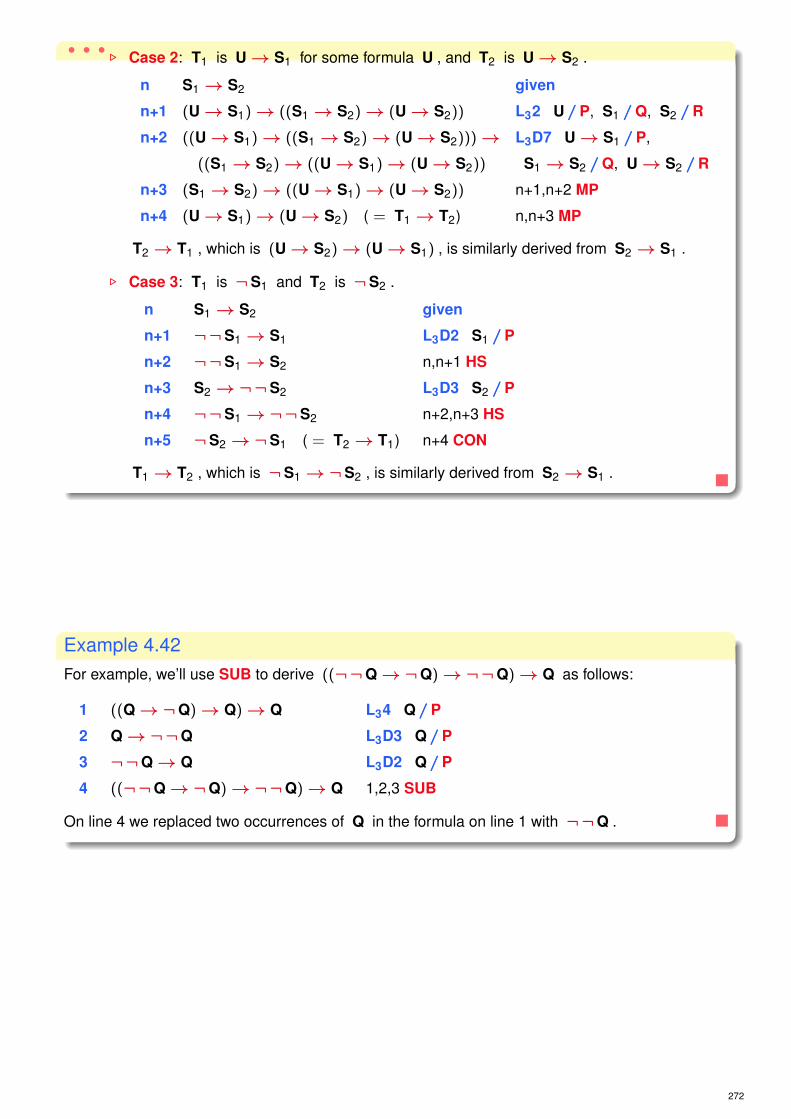
• • •. Case 2: T1 is U→ S1 for some formula U , and T2 is U→ S2 .

n S1→ S2 given

n+1 (U→ S1)→ ((S1→ S2)→ (U→ S2)) L32 U//P, S1 //Q, S2 //R

n+2 ((U→ S1)→ ((S1→ S2)→ (U→ S2)))→ L3D7 U→ S1 //P,

((S1→ S2)→ ((U→ S1)→ (U→ S2)) S1→ S2 //Q, U→ S2 //R

n+3 (S1→ S2)→ ((U→ S1)→ (U→ S2)) n+1,n+2 MP

n+4 (U→ S1)→ (U→ S2) ( = T1→ T2) n,n+3 MP

T2→ T1 , which is (U→ S2)→ (U→ S1) , is similarly derived from S2→ S1 .

. Case 3: T1 is ¬S1 and T2 is ¬S2 .

n S1→ S2 given

n+1 ¬¬S1→ S1 L3D2 S1 //P

n+2 ¬¬S1→ S2 n,n+1 HS

n+3 S2→¬¬S2 L3D3 S2 //P

n+4 ¬¬S1→¬¬S2 n+2,n+3 HS

n+5 ¬S2→¬S1 ( = T2→ T1) n+4 CON

T1→ T2 , which is ¬S1→¬S2 , is similarly derived from S2→ S1 .

Example 4.42For example, we’ll use SUB to derive ((¬¬Q→¬Q)→¬¬Q)→ Q as follows:

1 ((Q→¬Q)→ Q)→ Q L34 Q//P

2 Q→¬¬Q L3D3 Q//P

3 ¬¬Q→ Q L3D2 Q//P

4 ((¬¬Q→¬Q)→¬¬Q)→ Q 1,2,3 SUB

On line 4 we replaced two occurrences of Q in the formula on line 1 with ¬¬Q .

272

MODUS TOLLENS

MT (Modus Tollens). From ¬P and Q→ P derive ¬Q

m ¬P given

n Q→ P given

n+1 ¬¬Q→ Q L3D2 Q//P

n+2 ¬¬Q→ P n,n+1 HS

n+3 P→¬¬P L3D3 P//P

n+4 ¬¬Q→¬¬P n+2,n+3 HS

n+5 ¬P→¬Q n+4 CON

n+6 ¬Q m,n+5 MP

DN (Double Negation) From any formula R that contains P as a constituent,infer any formula R? that is the resultof replacing one or more occurrences of P in R with ¬¬P , and vice versa.

TRAN (Transposition) From any formula R that contains P→ (Q→ S) as a subformula,infer any formula R? that is the result of replacingone or more occurrences of P→ (Q→ S) in R with Q→ (P→ S) .

GCON (Generalized Contraposition) From any formula R that contains P→ Q as asubformula, infer any formula R? that is the result of replacing one or moreoccurrences of P→ Q in R with ¬Q→¬P , and vice versa.

Proof

DN follows from SUB and L3D2 and L3D3

TRAN follows from SUB and L3D7 .

GCON follows from SUB, L33 , and the fact that every formula of the form(P→ Q)→ (¬Q→¬P) is a theorem of L3A :

1 (¬¬P→¬¬Q)→ (¬Q→¬P) L33 ¬P//P, ¬Q//Q

2 (P→ Q)→ (¬Q→¬P) 1 DN (twice)

274

L3D8 . ¬(P→ Q)→ P

1 ¬P→ (P→ Q) L3D1 P//P, Q//Q

2 ¬P→¬¬(P→ Q) 1 DN

3 ¬(P→ Q)→ P 2 CON

GHS (Generalized Hypothetical Syllogism).From (P1→ (P2→ · · ·→ (Pn−1→ Pn) . . .) and Pn → Q ,infer (P1→ (P2→ · · ·→ (Pn−1→ Q) . . .)

I.B. n = 3 :

We show how to derive P1→ (P2→ Q) from P1→ (P2→ P3) and P3→ Q .

1 P1→ (P2→ P3) given

2 P3→ Q given

3 (P2→ P3)→ ((P3→ Q)→ (P2→ Q)) L32 P2 //P, P3 //Q, Q//R

4 (P3→ Q)→ ((P2→ P3)→ (P2→ Q)) 3 TRAN

5 (P2→ P3)→ (P2→ Q) 2,4 MP

6 P1→ (P2→ Q) 1,5 HS

276

I.H. From (P′1→ (P′2→ · · ·→ (P′n−2→ P′n−1 ) . . .) and P′n−1 → Q′

infer (P′1→ (P′2→ · · ·→ (P′n−2→ Q′ ) . . .)

I.S. Step from n − 1 to n : For arbitrary n > 3 , the derivation begins as

1 P1→ (P2→ (P3→ · · ·→ ( Pn−1→ Pn ) . . .)) given

2 Pn → Q given

3 (Pn−1→ Pn)→ ((Pn → Q)→ (Pn−1→ Q)) L32 Pn−1 //P, Pn //Q, Q//R

4 ((Pn → Q)→ ((Pn−1→ Pn)→ (Pn−1→ Q)) 3 TRAN

5 ( Pn−1→ Pn )→ ( Pn−1→ Q ) 2,4 MP

The formulas on lines 1 and 5 are, respectively, instances of the premissesP′1→ ((P′2→ (P′3 → · · ·→ (P′n−2→ P′n−1) . . .) and P′n−1→ Q′ of our I.H. with

. Pn−1→ Pn in place of P′n−1 , and

. Pn−1→ Q in place of Q′ , and

. Pi in place of P′i for 1 ≤ i ≤ n− 2

We finish the derivation with the instantiated conclusion of the I.H.

6 P1→ ((P2→ (P3→ · · ·→ ( Pn−1→ Q ) . . .) 1,5 I.H. (Pn−1→ Pn)//P′n−1,

(Pn−1→ Q)//Q′,

Pi //P′i for 1 ≤ i ≤ n− 2

GMP (Generalized Modus Ponens).From (P1→ (P2 → · · ·→ (Pn−1→ Pn) . . .) and one of the antecedents Pi , 1 ≤ i ≤ n − 1 ,infer the conditional that results from deleting Pi , the conditional arrow following Pi , andassociated parentheses.

Justification of GMP:

I By repeated applications of TRANthe antecedents P1, . . . ,Pn−1 can be permuted in any order.

I In particular, the antecedent Pi can be moved to the beginning of the formula,leaving the order of the other antecedents unchanged.

I At that point a single application of MP will produce the target formula with Pi removed.

278

CONSTRUCTIVE DILEMMA

In classical logic the argument P→ Q

¬P→ Q

Q

is valid (blue rows)

and the corresponding rule is derivable in CLA .

But the inference is not valid in L3 , if P and Q each have both the value � (red row)

Q P ((P → Q) (¬ P → Q)) Q

T T T T T ⊥ T T T T

T � � T T � � T T T

T ⊥ ⊥ T T T ⊥ T T T

� T T � � ⊥ T T � �� T � � � T � �� ⊥ ⊥ T � T ⊥ � � �⊥ T T ⊥ ⊥ ⊥ T T ⊥ ⊥⊥ � � � ⊥ � � � ⊥ ⊥⊥ ⊥ ⊥ T ⊥ T ⊥ ⊥ ⊥ ⊥

MODIFIED CONSTRUCTIVE DILEMMA

However, the argument P→ Q

(P→¬P)→ Q

Q

is valid in L3

and the corresponding rule is derivable in L3A . (green rows)

Q P ((P → Q) ((P → ¬ P) → Q)) Q

T T T T T T ⊥ ⊥ T T T T

T � � T T � T � � T T T

T ⊥ ⊥ T T ⊥ T T ⊥ T T T

� T T � � T ⊥ ⊥ T T � �� T � � T � � � � �� ⊥ ⊥ T � ⊥ T T ⊥ � � �⊥ T T ⊥ ⊥ T ⊥ ⊥ T T ⊥ ⊥⊥ � � � ⊥ � T � � ⊥ ⊥ ⊥⊥ ⊥ ⊥ T ⊥ ⊥ T T ⊥ ⊥ ⊥ ⊥

280

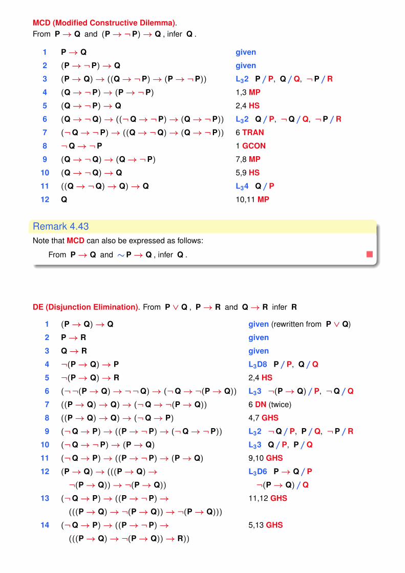
MCD (Modified Constructive Dilemma).From P→ Q and (P→¬P)→ Q , infer Q .

1 P→ Q given

2 (P→¬P)→ Q given

3 (P→ Q)→ ((Q→¬P)→ (P→¬P)) L32 P//P, Q//Q, ¬P//R

4 (Q→¬P)→ (P→¬P) 1,3 MP

5 (Q→¬P)→ Q 2,4 HS

6 (Q→¬Q)→ ((¬Q→¬P)→ (Q→¬P)) L32 Q//P, ¬Q//Q, ¬P//R

7 (¬Q→¬P)→ ((Q→¬Q)→ (Q→¬P)) 6 TRAN

8 ¬Q→¬P 1 GCON

9 (Q→¬Q)→ (Q→¬P) 7,8 MP

10 (Q→¬Q)→ Q 5,9 HS

11 ((Q→¬Q)→ Q)→ Q L34 Q//P

12 Q 10,11 MP

Remark 4.43Note that MCD can also be expressed as follows:

From P→ Q and ∼P→ Q , infer Q .

DE (Disjunction Elimination). From P ∨ Q , P→ R and Q→ R infer R

1 (P→ Q)→ Q given (rewritten from P ∨ Q)

2 P→ R given

3 Q→ R given

4 ¬(P→ Q)→ P L3D8 P//P, Q//Q

5 ¬(P→ Q)→ R 2,4 HS

6 (¬¬(P→ Q)→¬¬Q)→ (¬Q→¬(P→ Q)) L33 ¬(P→ Q)//P, ¬Q//Q

7 ((P→ Q)→ Q)→ (¬Q→¬(P→ Q)) 6 DN (twice)

8 ((P→ Q)→ Q)→ (¬Q→ P) 4,7 GHS

9 (¬Q→ P)→ ((P→¬P)→ (¬Q→¬P)) L32 ¬Q//P, P//Q, ¬P//R

10 (¬Q→¬P)→ (P→ Q) L33 Q//P, P//Q

11 (¬Q→ P)→ ((P→¬P)→ (P→ Q) 9,10 GHS

12 (P→ Q)→ (((P→ Q)→ L3D6 P→ Q//P

¬(P→ Q))→¬(P→ Q)) ¬(P→ Q)//Q

13 (¬Q→ P)→ ((P→¬P)→ 11,12 GHS

(((P→ Q)→¬(P→ Q))→¬(P→ Q)))

14 (¬Q→ P)→ ((P→¬P)→ 5,13 GHS

(((P→ Q)→¬(P→ Q))→ R))

15 ((P→ Q)→ Q)→ ((P→¬P)→ 8,14 HS

(((P→ Q)→¬(P→ Q))→ R))

16 ((P→ Q)→ Q)→ (((P→ Q)→ 15 TRAN

¬(P→ Q))→ ((P→¬P)→ R))

17 ((P→ Q)→¬(P→ Q))→ 16 TRAN

(((P→ Q)→ Q)→ ((P→¬P)→ R))

18 ((P→ Q)→¬(P→ Q))→ 17 TRAN

((P→¬P)→ (((P→ Q)→ Q)→ R))

19 (P→ Q)→ (((P→ Q)→ Q)→ Q) L3D6 P→ Q//P, Q//Q

20 (P→ Q)→ (((P→ Q)→ Q)→ R) 3,19 GHS

21 (((P→ Q)→ Q)→ R)→ L31 ((P→ Q)→ Q)→ R//P,

((P→¬P)→ (((P→ Q)→ Q)→ R)) P→¬P//Q

22 (P→ Q)→ ((P→¬P)→ 20,21 HS

(((P→ Q)→ Q)→ R))

23 (P→¬P)→ (((P→ Q)→ Q)→ R) 18,22 MCD

24 R→ (((P→ Q)→ Q)→ R) L31 R//P, (P→ Q)→ Q//R

25 P→ (((P→ Q)→ Q)→ R) 2,24 HS

26 ((P→ Q)→ Q)→ R 23,25 MCD

27 R 1,26 MP

DC (Disjunctive Consequence). From P→ R and Q→ R infer (P ∨ Q)→ R

Implicit in lines 2–26 of the previous derivation.

L3D9 . (P ∨ Q)→ (Q ∨ P) (rewritten to ((P→ Q)→ Q)→ ((Q→ P)→ P) )

1 P→ ((Q→ P)→ P) L31 P//P, Q→ P//Q

2 Q→ ((Q→ P)→ P) L3D6 Q//P, P//Q

3 ((P→ Q)→ Q)→ ((Q→ P)→ P) 1,2 DC

284

L3D10 . (P→ Q) ∨ (Q→ P) (rewritten to ((P→ Q)→ (Q→ P))→ (Q→ P) )

1 ((P→ Q)→ (Q→ P))→ L32 P→ Q//P,

(((Q→ P)→ P)→ ((P→ Q)→ P)) Q→ P//Q, P//R

2 ((P→ Q)→ Q)→ ((Q→ P)→ P) L3D9 P//P, Q//Q

3 ((Q→ P)→ P)→ ((P→ Q)→ Q) L3D9 Q//P, P//Q

4 ((P→ Q)→ (Q→ P))→ 1,2,3 SUB

(((P→ Q)→ Q)→ ((P→ Q)→ P))

5 (((P→ Q)→ (Q→ P))→ L32 (P→ Q)→ (Q→ P)//P,

(((P→ Q)→ Q)→ ((P→ Q)→ P)))→ ((P→ Q)→ Q)→(((((P→ Q)→ Q)→ ((P→ Q)→ P))→ ((P→ Q)→ P)//Q,

((Q→ (P→ Q))→ (Q→ P)))→ (Q→ (P→ Q))→(((P→ Q)→ (Q→ P))→ (Q→ P)//R

((Q→ (P→ Q))→ (Q→ P))))

6 (((P→ Q)→ Q)→ ((P→ Q)→ P))→ 4,5 MP

((Q→ (P→ Q))→ (Q→ P))→(((P→ Q)→ (Q→ P))→

((Q→ (P→ Q))→ (Q→ P)))

7 ((¬Q→¬(P→ Q))→ (¬P→¬(P→ Q)))→ L3D4 (¬Q→¬(P→ Q))→((¬Q→¬(P→ Q))→ (¬P→¬(P→ Q))) (¬P→¬(P→ Q))//P

8 ((¬Q→¬(P→ Q))→ (¬P→¬(P→ Q)))→ 7 TRAN

(¬P→ ((¬Q→¬(P→ Q))→¬(P→ Q)))

9 ((¬Q→¬(P→ Q))→¬(P→ Q))→ L3D9 ¬Q//P, ¬(P→ Q)//Q

((¬(P→ Q)→¬Q)→¬Q)

10 ((¬Q→¬(P→ Q))→ (¬P→¬(P→ Q)))→ 8,9 GHS

(¬P→ ((¬(P→ Q)→¬Q)→¬Q))

11 ((¬Q→¬(P→ Q))→ (¬P→¬(P→ Q)))→ 10 TRAN

((¬(P→ Q)→¬Q)→ (¬P→¬Q))

12 ((P→ Q)→ Q)→ ((P→ Q)→ P)→ 11 GCON (four times)

((Q→ (P→ Q))→ (Q→ P))

13 ((P→ Q)→ (Q→ P))→ 4,12 HS

((Q→ (P→ Q))→ (Q→ P))

14 ((Q→ (P→ Q))→ 13 TRAN

(((P→ Q)→ (Q→ P))→ (Q→ P)))

15 Q→ (P→ Q) L31 Q//P, P//Q

16 ((P→ Q)→ (Q→ P))→ (Q→ P) 14,15 MP

286

L3D11 (P→ (P→ (P→ Q)))→ (P→ (P→ Q))

1 ¬P→ (P→ Q) L3D1 P//P, Q//Q

2 (P→¬P)→ L32 P//P, ¬P//Q, P→ Q//R

((¬P→ (P→ Q))→ (P→ (P→ Q)))

3 (P→¬P)→ (P→ (P→ Q)) 1,2 GMP

4 ((P→¬P)→ (P→ (P→ Q)))→ L32 P→¬P//P,

(((P→ (P→ Q))→ P)→ ((P→¬P)→ P)) P→ (P→ Q)//Q, P//R

5 ((P→ (P→ Q))→ P)→ ((P→¬P)→ P) 3,4 MP

6 ((P→¬P)→ P)→ P L34 P//P

7 ((P→ (P→ Q))→ P)→ P 5,6 HS

8 (((P→ (P→ Q))→ P)→ P)→ L3D9 P→ (P→ Q)//P, P//Q

((P→ (P→ (P→ Q)))→ (P→ (P→ Q)))

9 (P→ (P→ (P→ Q)))→ (P→ (P→ Q)) 7,8 MP

CI (Conjunction Introduction). From P and Q , infer P ∧ Q

1 P Assumption

2 Q Assumption

3 ¬¬P 1 DN

4 ¬¬P→ (¬P→¬Q) L3D1 ¬P//P, ¬Q//Q

5 ¬P→¬Q 3,4 MP

6 (¬P→¬Q)→ L3D6 ¬P→¬Q//P, ¬Q//Q

(((¬P→¬Q)→¬Q)→¬Q)

7 ((¬P→¬Q)→¬Q)→¬Q 5,6 MP

8 ¬¬Q→¬((¬P→¬Q)→¬Q) 7 GCON

9 ¬¬Q 2 DN

10 ¬((¬P→¬Q)→¬Q) 8,9 MP (rewritten from P ∧ Q)

288

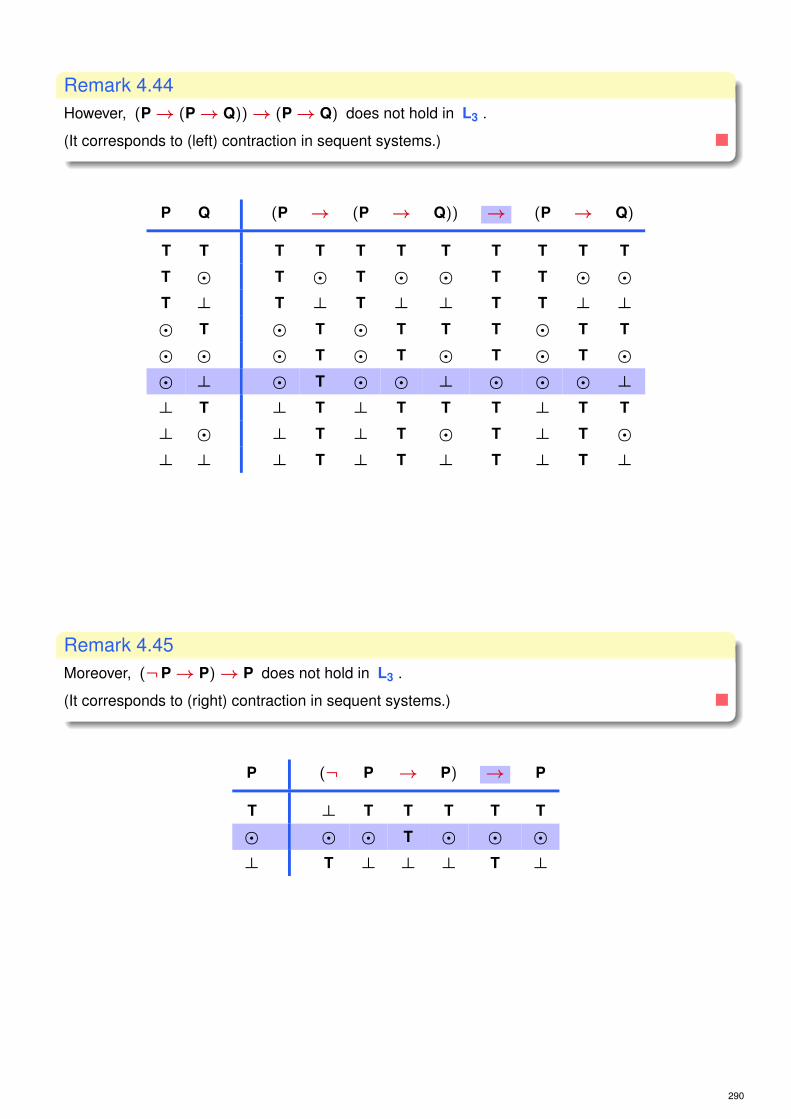
Remark 4.44However, (P→ (P→ Q))→ (P→ Q) does not hold in L3 .

(It corresponds to (left) contraction in sequent systems.)

P Q (P → (P → Q)) → (P → Q)


T � T � T � � T T � �T ⊥ T ⊥ T ⊥ ⊥ T T ⊥ ⊥� T � T � T T T � T T

� � � T � T � T � T �� ⊥ � T � � ⊥ � � � ⊥⊥ T ⊥ T ⊥ T T T ⊥ T T

⊥ � ⊥ T ⊥ T � T ⊥ T �⊥ ⊥ ⊥ T ⊥ T ⊥ T ⊥ T ⊥

Remark 4.45Moreover, (¬P→ P)→ P does not hold in L3 .

(It corresponds to (right) contraction in sequent systems.)

P (¬ P → P) → P

T ⊥ T T T T T

� � � T � � �⊥ T ⊥ ⊥ ⊥ T ⊥

290

Remark 4.46The familiar Deduction Theorem:

If S ∪ {F } ` G , then S ` F→ G

does not hold in L3A .

Example 4.47Whenever P ∧ ((P→ Q) ∧ (P→ (Q→ R))) is true in L3 so is R ,but (P ∧ ((P→ Q) ∧ (P→ (Q→ R))))→ R is no L3 -tautology. (see next slide)

Proof: We may derive R from P ∧ ((P→ Q) ∧ (P→ (Q→ R)))

1 P ∧ ((P→ Q) ∧ (P→ (Q→ R))) Assumption

2 P 1 LSIMP

3 (P→ Q) ∧ (P→ (Q→ R)) 1 RSIMP

4 (P→ Q) 3 LSIMP

5 (P→ (Q→ R)) 3 RSIMP

6 (Q→ R) 2,5 MP

7 (P→ R) 4,6 HS

8 R 2,7 MP

P Q R (P ∧ ((P → Q) ∧ (P → (Q → R)))) → R

T T T T T T T T T T T T T T T TT T � T � T T T � T � T � � T �T T ⊥ T ⊥ T T T ⊥ T ⊥ T ⊥ ⊥ T ⊥T � T T � T � � � T T � T T T TT � � T � T � � � T T � T � T �T � ⊥ T � T � � � T � � � ⊥ � ⊥T ⊥ T T ⊥ T ⊥ ⊥ ⊥ T T ⊥ T T T TT ⊥ � T ⊥ T ⊥ ⊥ ⊥ T T ⊥ T � T �T ⊥ ⊥ T ⊥ T ⊥ ⊥ ⊥ T T ⊥ T ⊥ T ⊥� T T � � � T T T � T T T T T T� T � � � � T T T � T T � � T �� T ⊥ � � � T T � � � T ⊥ ⊥ � ⊥� � T � � � T � T � T � T T T T� � � � � � T � T � T � T � T �� ⊥ � � � T � T � T � � ⊥ � ⊥� ⊥ T � � � � ⊥ � � T ⊥ T T T T� ⊥ � � � � � ⊥ � � T ⊥ T � T �� ⊥ ⊥ � � � � ⊥ � � T ⊥ T ⊥ � ⊥⊥ T T ⊥ ⊥ ⊥ T T T ⊥ T T T T T T⊥ T � ⊥ ⊥ ⊥ T T T ⊥ T T � � T �⊥ T ⊥ ⊥ ⊥ ⊥ T T T ⊥ T T ⊥ ⊥ T ⊥⊥ � T ⊥ ⊥ ⊥ T � T ⊥ T � T T T T⊥ � � ⊥ ⊥ ⊥ T � T ⊥ T � T � T �⊥ � ⊥ ⊥ ⊥ ⊥ T � T ⊥ T � � ⊥ T ⊥⊥ ⊥ T ⊥ ⊥ ⊥ T ⊥ T ⊥ T ⊥ T T T T⊥ ⊥ � ⊥ ⊥ ⊥ T ⊥ T ⊥ T ⊥ T � T �⊥ ⊥ ⊥ ⊥ ⊥ ⊥ T ⊥ T ⊥ T ⊥ T ⊥ T ⊥

292

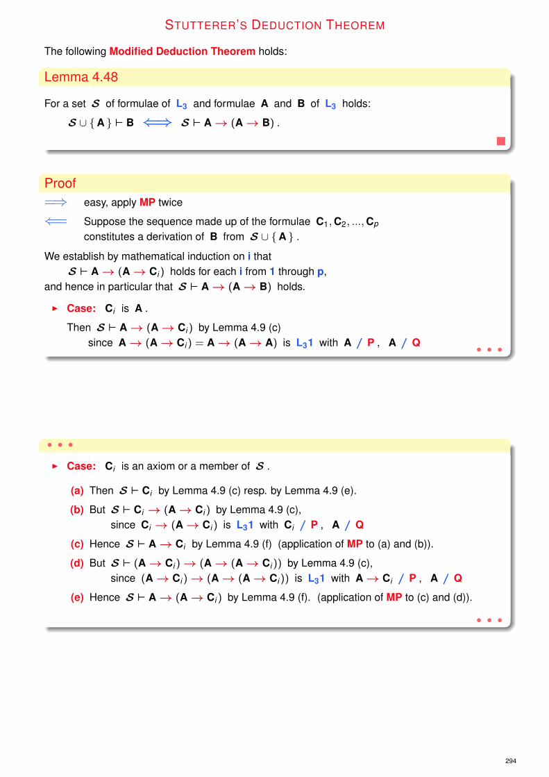
STUTTERER’S DEDUCTION THEOREM

The following Modified Deduction Theorem holds:

Lemma 4.48

For a set S of formulae of L3 and formulae A and B of L3 holds:

S ∪ {A } ` B ⇐⇒ S ` A→ (A→ B) .

Proof=⇒ easy, apply MP twice

⇐= Suppose the sequence made up of the formulae C1,C2, ...,Cp

constitutes a derivation of B from S ∪ {A } .

We establish by mathematical induction on i thatS ` A→ (A→ Ci ) holds for each i from 1 through p,

and hence in particular that S ` A→ (A→ B) holds.

I Case: Ci is A .

Then S ` A→ (A→ Ci ) by Lemma 4.9 (c)since A→ (A→ Ci ) = A→ (A→ A) is L31 with A // P , A // Q • • •

• • •

I Case: Ci is an axiom or a member of S .

(a) Then S ` Ci by Lemma 4.9 (c) resp. by Lemma 4.9 (e).

(b) But S ` Ci → (A→ Ci ) by Lemma 4.9 (c),since Ci → (A→ Ci ) is L31 with Ci // P , A // Q

(c) Hence S ` A→ Ci by Lemma 4.9 (f) (application of MP to (a) and (b)).

(d) But S ` (A→ Ci )→ (A→ (A→ Ci )) by Lemma 4.9 (c),since (A→ Ci )→ (A→ (A→ Ci )) is L31 with A→ Ci // P , A // Q

(e) Hence S ` A→ (A→ Ci ) by Lemma 4.9 (f). (application of MP to (c) and (d)).

• • •

294

• • •

I Case: Ci is obtained by MP from Ch and Ch → Ci .

Then S ` A→ (A→ Ch) and S ` A→ (A→ (Ch → Ci )) hold by I.H.

n A→ (A→ Ch)...

m A→ (A→ (Ch → Ci ))

m+1 A→ (Ch → (A→ Ci )) m TRAN

m+2 Ch → (A→ (A→ Ci )) m+1 TRAN

m+3 A→ (A→ (A→ (A→ Ci ))) n,m+2 GHS

m+4 (A→ (A→ (A→ (A→ Ci ))))→ L3D11 A//P, A→ Ci //Q

(A→ (A→ (A→ Ci )))

m+5 A→ (A→ (A→ Ci )) m+3, m+4 MP

m+6 (A→ (A→ (A→ Ci )))→ (A→ (A→ Ci )) L3D11 A//P, Ci //Q

m+7 A→ (A→ Ci ) m+6, m+7 MP

Hence S ` A→ (A→ Ci ) by Lemma 4.9.

Example 4.49

R is derivable from P ∧ ((P→ Q) ∧ (P→ (Q→ R))) in L3A . (cf. Example 4.47)

Consequently, it follows from the Modified Deduction Theorem that

(P ∧ ((P→ Q) ∧ (P→ (Q→ R))))→ ((P ∧ ((P→ Q) ∧ (P→ (Q→ R))))→ R)

is a theorem! (see truth table on the next slide)

296

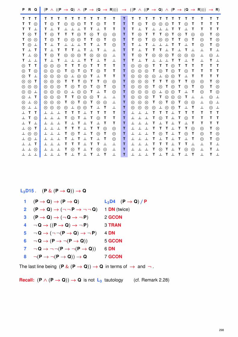
P R Q(P ∧ ((P → Q) ∧ (P → (Q → R)))

)→ (

(P ∧ ((P → Q) ∧ (P → (Q → R)))

)→ R)

T T T T T T T T T T T T T T T T T T T T T T T T T T T TT T � T � T � � � T T � T T T T � T � � � T T � T T T TT T ⊥ T ⊥ T ⊥ ⊥ ⊥ T T ⊥ T T T T ⊥ T ⊥ ⊥ ⊥ T T ⊥ T T T TT � T T � T T T � T � T � � T T � T T T � T � T � � T �T � � T � T � � � T T � T � T T � T � � � T T � T � T �T � ⊥ T ⊥ T ⊥ ⊥ ⊥ T T ⊥ T � T T ⊥ T ⊥ ⊥ ⊥ T T ⊥ T � T �T ⊥ T T ⊥ T T T ⊥ T ⊥ T ⊥ ⊥ T T ⊥ T T T ⊥ T ⊥ T ⊥ ⊥ T ⊥T ⊥ � T � T � � � T � � � ⊥ T T � T � � � T � � � ⊥ � ⊥T ⊥ ⊥ T ⊥ T ⊥ ⊥ ⊥ T T ⊥ T ⊥ T T ⊥ T ⊥ ⊥ ⊥ T T ⊥ T ⊥ T ⊥� T T � � � T T T � T T T T T � � � T T T � T T T T T T� T � � � � T � T � T � T T T � � � T � T � T � T T T T� T ⊥ � � � � ⊥ � � T ⊥ T T T � � � � ⊥ � � T ⊥ T T T T� � T � � � T T T � T T � � T � � � T T T � T T � � T �� T � T � T � T � T � � � T � T � T � T � T �� ⊥ � � � � ⊥ � � T ⊥ T � T � � � � ⊥ � � T ⊥ T � T �� ⊥ T � � � T T � � � T ⊥ ⊥ T � � � T T � � � T ⊥ ⊥ � ⊥� ⊥ � � � � T � T � T � � ⊥ T � � � T � T � T � � ⊥ � ⊥� ⊥ ⊥ � � � � ⊥ � � T ⊥ T ⊥ T � � � � ⊥ � � T ⊥ T ⊥ � ⊥⊥ T T ⊥ ⊥ ⊥ T T T ⊥ T T T T T ⊥ ⊥ ⊥ T T T ⊥ T T T T T T⊥ T � ⊥ ⊥ ⊥ T � T ⊥ T � T T T ⊥ ⊥ ⊥ T � T ⊥ T � T T T T⊥ T ⊥ ⊥ ⊥ ⊥ T ⊥ T ⊥ T ⊥ T T T ⊥ ⊥ ⊥ T ⊥ T ⊥ T ⊥ T T T T⊥ � T ⊥ ⊥ ⊥ T T T ⊥ T T � � T ⊥ ⊥ ⊥ T T T ⊥ T T � � T �⊥ � � ⊥ ⊥ ⊥ T � T ⊥ T � T � T ⊥ ⊥ ⊥ T � T ⊥ T � T � T �⊥ � ⊥ ⊥ ⊥ ⊥ T ⊥ T ⊥ T ⊥ T � T ⊥ ⊥ ⊥ T ⊥ T ⊥ T ⊥ T � T �⊥ ⊥ T ⊥ ⊥ ⊥ T T T ⊥ T T ⊥ ⊥ T ⊥ ⊥ ⊥ T T T ⊥ T T ⊥ ⊥ T ⊥⊥ ⊥ � ⊥ ⊥ ⊥ T � T ⊥ T � � ⊥ T ⊥ ⊥ ⊥ T � T ⊥ T � � ⊥ T ⊥⊥ ⊥ ⊥ ⊥ ⊥ ⊥ T ⊥ T ⊥ T ⊥ T ⊥ T ⊥ ⊥ ⊥ T ⊥ T ⊥ T ⊥ T ⊥ T ⊥

L3D15 . (P & (P→ Q))→ Q

1 (P→ Q)→ (P→ Q) L3D4 (P→ Q)//P

2 (P→ Q)→ (¬¬P→¬¬Q) 1 DN (twice)

3 (P→ Q)→ (¬Q→¬P) 2 GCON

4 ¬Q→ ((P→ Q)→¬P) 3 TRAN

5 ¬Q→ (¬¬(P→ Q)→¬P) 4 DN

6 ¬Q→ (P→¬(P→ Q)) 5 GCON

7 ¬Q→¬¬(P→¬(P→ Q)) 6 DN

8 ¬(P→¬(P→ Q))→ Q 7 GCON

The last line being (P & (P→ Q))→ Q in terms of → and ¬ .

Recall: (P ∧ (P→ Q))→ Q is not L3 tautology (cf. Remark 2.28)

298

L3D16 . (P→ Q)→ ((R→ S)→ ((P & R)→ (Q & S)))

(see [Rothenberg, 2005, A.21])


COMPLETENESS OF 3-VALUED ŁUKASIEWICZ’S LOGIC

Remark 4.50Recall:

I We abbreviated the formula ¬(p1→ p1) as f (cf. Definition 2.16)

I We abbreviate formulas of the form (A→¬A) as ∼A ( = Bochvar’s ∼A )

Recall: A A → ¬ A ∼A

T T ⊥ ⊥ T ⊥� � T � � T

⊥ ⊥ T T ⊥ T

ADDITIONAL DERIVED FORMULAE

L3D30 ` (A→∼A)→∼A

L3D31 ∼∼A→ A

L3D32 (A→ B)→ (¬B→¬A)

L3D33 ¬(A→ B)→¬B

L3D34 A→ (¬B→¬(A→ B))

L3D35 ` ∼A→ (∼¬B→ (A→ B))

302

L3D30 (A→∼A)→∼A

1 (((A→¬A)→ A)→ A)→ ((A→ (A→¬A))→ L32 (A→¬A)→ A//P,(((A→¬A)→ A)→ (A→¬A))) A//Q, A→¬A//R

2 ((A→¬A)→ A)→ A L34 A//P

3 (A→ (A→¬A))→ (((A→¬A)→ A)→ (A→¬A)) 1,2 MP

4 ¬A→ (A→¬A) L31 ¬A//P, A//Q

5 ¬A→¬¬(A→¬A) 4 DN

6 ¬(A→¬A)→ A 5 CON

7 ((A→¬A)→¬(A→¬A))→ L32 A→¬A//P,((¬(A→¬A)→ A)→ ((A→¬A)→ A)) ¬(A→¬A)//Q, A//R

8 ((A→¬A)→¬(A→¬A))→ ((A→¬A)→ A) 6,7 GMP

9 ((A→¬A)→ A)→ ((A→ (A→¬A))→ (A→¬A)) 3 TRAN

10 ((A→¬A)→¬(A→¬A))→ 8,9 GHS(A→ (A→¬A))→ ((A→¬A))

11 (A→ (A→¬A))→ 10 TRAN(((A→¬A)→¬(A→¬A))→ (A→¬A))

12 (((A→¬A)→¬(A→¬A))→ L34 A→¬A//P

(A→¬A))→ (A→¬A)

13 (A→ (A→¬A))→ (A→¬A)) 11,12 GHS

L3D31 ∼∼A→ A

1 ¬(A→¬A)→ A L3D8 A//P, ¬A//Q

2 ((A→¬A)→¬(A→¬A))→ L32 A→¬A//P

((¬(A→¬A)→ A)→ ¬(A→¬A)//Q, A//R

((A→¬A)→ A))

3 (¬(A→¬A)→ A)→ 2 TRAN

(((A→¬A)→¬(A→¬A))→((A→¬A)→ A))

4 ((A→¬A)→¬(A→¬A))→ 1,3 MP

((A→¬A)→ A)

5 ((A→¬A)→ A)→ A L34 A//P

6 ((A→¬A)→¬(A→¬A))→ A 4,5 HS

The other direction does not hold! A A → ∼ ∼ A

T T T T ⊥ T

� � � ⊥ T �⊥ ⊥ T ⊥ T ⊥

304

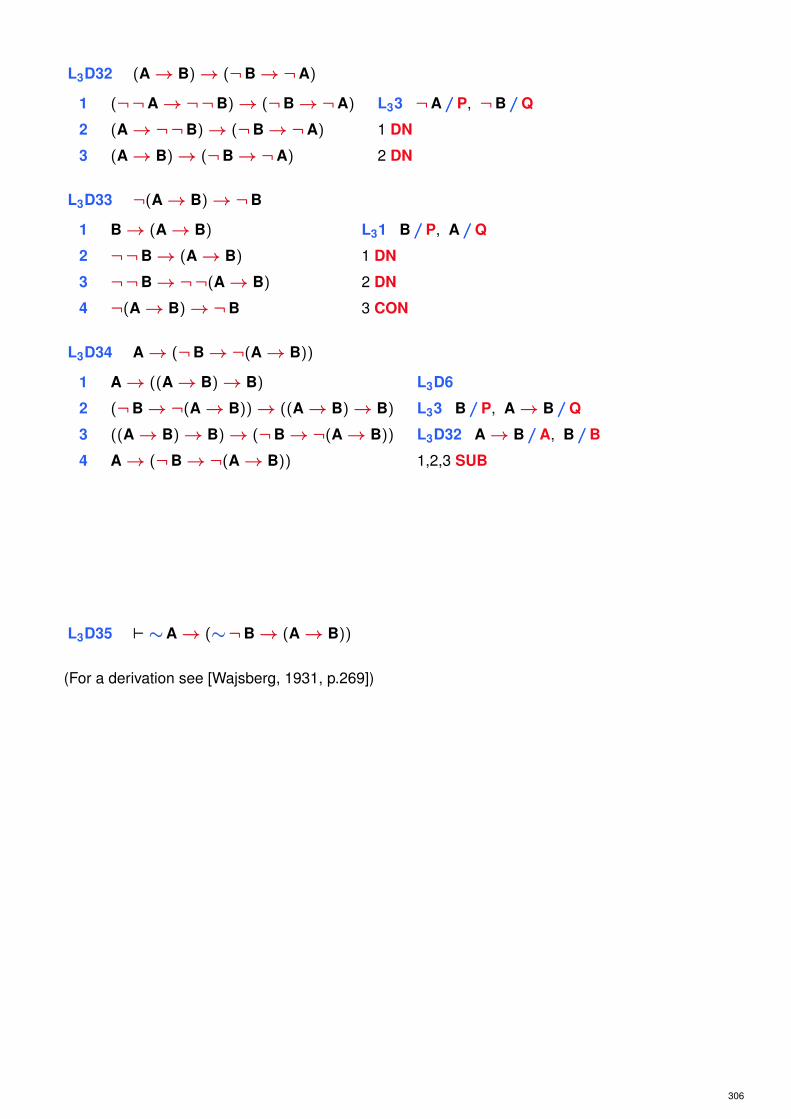
L3D32 (A→ B)→ (¬B→¬A)

1 (¬¬A→¬¬B)→ (¬B→¬A) L33 ¬A//P, ¬B//Q

2 (A→¬¬B)→ (¬B→¬A) 1 DN

3 (A→ B)→ (¬B→¬A) 2 DN

L3D33 ¬(A→ B)→¬B

1 B→ (A→ B) L31 B//P, A//Q

2 ¬¬B→ (A→ B) 1 DN

3 ¬¬B→¬¬(A→ B) 2 DN

4 ¬(A→ B)→¬B 3 CON

L3D34 A→ (¬B→¬(A→ B))

1 A→ ((A→ B)→ B) L3D6

2 (¬B→¬(A→ B))→ ((A→ B)→ B) L33 B//P, A→ B//Q

3 ((A→ B)→ B)→ (¬B→¬(A→ B)) L3D32 A→ B//A, B//B

4 A→ (¬B→¬(A→ B)) 1,2,3 SUB

L3D35 ` ∼A→ (∼¬B→ (A→ B))

(For a derivation see [Wajsberg, 1931, p.269])

306

Lemma 4.51

(a) If S is syntactically inconsistent, then S ` A for every formula A in L3 .

(b) S is syntactically inconsistent if and only if S ` f .

(c) If S ∪ {A } is syntactically inconsistent, then S ` ∼A . (Recall: ∼A = A→¬A )

(d) If S ∪ {∼A } is syntactically inconsistent, then S ` A

Proof(a) Suppose S ` B and S ` ¬B for some formula B of L3 . We get:

1 B given

2 ¬B given

3 ¬B→ (B→ A) L3D1 B//P, A//Q

4 B→ A 2,3 MP

5 A 1,4 MP

This implies S ` A for any formula A of L3 .

• • •

• • •

(b) ⇐= On the one hand, we get p1→ p1 as instance of L3D4 : P→ PNow with Lemma 4.9 (b) we get S ` p1→ p1 andthen S ` ¬¬(p1→ p1) with L3D3 : P→¬¬PThis means: S ` ¬ f

Hence, if S ` f holds as well, then S is syntactically inconsistent.

=⇒ If S is syntactically inconsistent then we get S ` f as special case ofLemma 4.51 (a) with A = f .

(c) Suppose S ∪ {A } is syntactically inconsistent.Then S ∪ {A } ` ¬A by Lemma 4.51 (a) (with ¬A as arbitrary formula),hence S ` A→ (A→¬A) by Lemma 4.48 (Stutterer’s DT)In other words: S ` A→∼A)

Hence S ` ∼A by L3D30 : (A→∼A)→∼A and Lemma 4.9 (f) (MP).

(d) With Lemma 4.51 (c),

we get S ` ∼∼A ( = ∼ (A→¬A) = (A→¬A)→¬(A→¬A) )

With L3D31 : ∼∼A→ Awe get S ` A with Lemma 4.9 (f) (MP).

308

Remark 4.52For the proof that

if a set S of formulas of L3 is syntactically consistent,then S is semantically consistent as well,

we proceed as follows:

I At first we proceed as with the two-valued precedent:i.e., we assume S to be syntactically consistentand then extend S into a superset S∞ by iteratively adding formulaewhile preserving consistency.

I The formulae of S∞ , and hence those of S ,will thereafter be shown to evaluate to > under some suitably constructed interpretation.

Definition 4.53Given a syntactically consistent set S of formulas of L3 .

We construct a set S∞ of formulas of L3 as follows:

1. We define S0 as S ,

2. We assume the formulas of L3 to be alphabetically orderedand Ai to be for each i from 1 on the alphabetically i -th formula of L3 ,

and define S i =

S i−1 ∪ {Ai } if S i−1 ∪ {Ai } is syntactically consistent

S i−1 otherwise

3. We define S∞ as⋃

i∈N S i .

Lemma 4.54

For S∞ the following holds:

(a) S∞ is syntactically consistent

(b) S∞ is maximally consistent

310

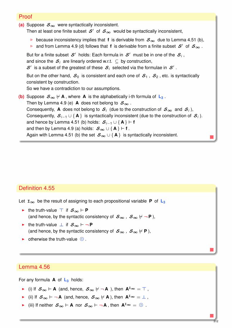
Proof(a) Suppose S∞ were syntactically inconsistent.

Then at least one finite subset S′ of S∞ would be syntactically inconsistent,

. because inconsistency implies that f is derivable from S∞ due to Lemma 4.51 (b),

. and from Lemma 4.9 (d) follows that f is derivable from a finite subset S′ of S∞ .

But for a finite subset S′ holds: Each formula in S′ must be in one of the S i ,and since the S i are linearly ordered w.r.t. ⊆ by construction,S′ is a subset of the greatest of these S i selected via the formulae in S′ .

But on the other hand, S0 is consistent and each one of S1 , S2 , etc. is syntacticallyconsistent by construction.So we have a contradiction to our assumptions.

(b) Suppose S∞ 6` A , where A is the alphabetically i-th formula of L3 .Then by Lemma 4.9 (e) A does not belong to S∞ .Consequently, A does not belong to S i (due to the construction of S∞ and S i ),Consequently, S i−1 ∪ {A } is syntactically inconsistent (due to the construction of S i ).and hence by Lemma 4.51 (b) holds: S i−1 ∪ {A } ` fand then by Lemma 4.9 (a) holds: S∞ ∪ {A } ` f .Again with Lemma 4.51 (b) the set S∞ ∪ {A } is syntactically inconsistent.

Definition 4.55

Let I∞ be the result of assigning to each propositional variable P of L3

I the truth-value > if S∞ ` P(and hence, by the syntactic consistency of S∞ , S∞ 6` ¬P ),

I the truth-value ⊥ if S∞ ` ¬P(and hence, by the syntactic consistency of S∞ , S∞ 6` P ),

I otherwise the truth-value � .

Lemma 4.56

For any formula A of L3 holds:

I (i) If S∞ ` A (and, hence, S∞ 6` ¬A ), then AI∞ = > ,

I (ii) If S∞ ` ¬A (and, hence, S∞ 6` A ), then AI∞ = ⊥ ,

I (iii) If neither S∞ ` A nor S∞ ` ¬A , then AI∞ = � .

312

ProofProof by mathematical induction on the length `(A) of A . (Step from k < n to n )

We define the length `(A) of a formula A as follows:

I `(P) of a propositional variable P is 1

I `(¬A) of a negation ¬A is `(A) + 1

I `(A→ B) of a conditional A→ B is `(A) + `(B) + 1

I.B. `(A) = 1 , and hence A is a propositional variable.Then the assertion holds by the very construction of I∞ in Definition 4.55.

I.H. Lemma 4.56 holds for formulae F with `(F) < `(A) .

I.S. `(A) > 1 .

We consider as Case 1 and Case 2that A is either a negation ¬B or a conditional B→ C .

For both cases we have to consider the subcases (i)-(iii):S∞ ` A , S∞ ` ¬A and that neither of these two derivations exists.

For these subcases (i)-(iii) we have to show AI∞ = > , AI∞ = ⊥ and AI∞ = �respectively.

• • •

• • •

Case 1: A is a negation ¬B .

(i) Suppose S∞ ` ¬B .

Then S∞ 6` B , since S∞ is consistent.Consequently, I.H. (ii): BI∞ = ⊥ , and hence [¬B]I∞ = > .

(ii) Suppose S∞ ` ¬¬B .

Then by L3D2 and Lemma 4.9 (f) follows: S∞ ` B ,hence by I.H. BI∞ = > , and hence [¬B]I∞ = ⊥ .

(iii) Suppose neither S∞ ` ¬B nor S∞ ` ¬¬B .

If B were provable from S∞ ,then by L3D3 and Lemma 4.9 (f) follows:¬¬B would be provable from S∞ . Contradiction

Hence neither S∞ ` B nor S∞ ` ¬B .

With I.H. follows: BI∞ = � , and consequently, [¬B]I∞ = � .

• • •

314

• • •

Case 2: A is a conditional B→ C .

(i) Suppose S∞ ` B→ C .

. If S∞ ` ¬B , then BI∞ = ⊥ by I.H..

. If S∞ ` C , then CI∞ = > by I.H..

. If S∞ ` B , then S∞ ` C by Lemma 4.9 (f), and hence again CI∞ = > .

. If S∞ ` ¬C , then S∞ ` ¬B by Lemma 4.9 (1), L3D32 and Lemma 4.9 (f),and hence again BI∞ = ⊥ .

Consequently,

. if any one of B , ¬B , C , and ¬C is provable from S∞ ,then BI∞ = ⊥ or CI∞ = > , and therefore: (B→ C)I∞ = > .

. If none of B , ¬B , C , and ¬C is provable from S∞ ,then BI∞ = CI∞ = � by I.H., and therefore: (B→ C)I∞ = > .

(ii) Suppose S∞ ` ¬(B→ C) .From ¬(B→ C) follows B with L3D8 and ¬C with L3D33 ,and with Lemma 4.9 (f) we get both S∞ ` B and S∞ ` ¬C .With I.H. this implies BI∞ = > and CI∞ = ⊥ , and hence (B→ C)I∞ = ⊥ .

• • •

• • •

(iii) Suppose neither S∞ ` (B→ C) nor S∞ ` ¬(B→ C) .Then ¬B nor C can be provable from S∞ , because

. with L3D1 ( ¬P→ (P→ Q) ), Lemma 4.9 (a), and Lemma 4.9 (f)we would then get the contradiction that (B→ C) is provable from S∞ .

. with L33 we would prove S∞ ` (B→ C) from S∞ ` C

Then BI∞ cannot be equal to ⊥ nor CI∞ can be equal to > ,

. because in case of S∞ 6` ¬B we would get– either S∞ ` B and then BI∞ = > due to I.H.– or S∞ 6` B and then BI∞ = � due to I.H.

. and analogously in case of S∞ 6` C .

• • •

316

• • •

. Now suppose first that BI∞ = > .

Then CI∞ cannot equal ⊥ , for by I.H. ¬C would then be provable from S∞ ,and hence by L3D34 and Lemma 4.9 (f) so would ¬(B→ C) be.Since as shown above, CI∞ cannot be equal to> ,CI∞ must equal � , and hence (B→ C)I∞ = � .

. Suppose next that BI∞ = � .

We assume that CI∞ is also equal to � .Then by I.H. neither B nor ¬C would be provable from S∞ ,Consequently, by the maximal consistency of S∞ both S ∪ {B } and S ∪ {¬C }would be syntactically inconsistent,hence by Lemma 4.51 (c) both ∼B and ∼¬C would be provable from S∞ ,and hence by L3D35 and Lemma 4.9 (f) so would (B→ C) be.

Since as shown above, CI∞ cannot be equal to > ,hence CI∞ must equal ⊥ , and hence (B→ C)I∞ = � .

Lemma 4.57

If S is syntactically consistent, then S is semantically consistent.

ProofSince every member of S belongs to S∞and hence by Lemma 4.9 (e) is provable from S∞ ,every member of S is thus sure to evaluate to > under I∞ .

318

COMPLETENESS THEOREM

Theorem 4.58

For every set S of formulae of L3 and every formula A of L3 holds:

I If S |= A , then S ` A . (Strong Completeness Theorem)

I If |= A , then ` A . (Weak Completeness Theorem)

ProofSuppose S |= A .Then S ∪ {∼A } is semantically inconsistent,

because A would be true in every model of S ,therefore ¬A would be false in every model of S , and so would be ∼A = A→¬A .

Consequently, by Lemma 4.57 we ge that S ∪ {∼A } is syntactically inconsistent,and hence by Lemma 4.51 (d) S ` A .

For the special case of S as ∅ , we get the Weak Completeness Theorem.

DECIDABILITY

Lemma 4.59The set of theorems of L3A is decidable.

ProofThis holds because L3A is a sound and complete system for L3 ,and the set of tautologies in L3 is decidable on the basis of the construction of truth-tables.

320


Remark 4.60One of the first applications of many valued logics was for proofs of independence

Consider the following axiom system K for classical propositional logic

Ax1 p1→ (p2→ p1)

Ax2 ((p1→ p2)→ p1)→ p1Ax3 (p1→ p2)→ ((p2→ p3)→ (p1→ p3))

Ax4 (p1 ∧ p2)→ p1Ax5 (p1 ∧ p2)→ p2Ax6 (p1→ p2)→ ((p1→ p3)→ p1→ p2 ∧ p3))

Ax7 p1→ (p1 ∨ p2)

Ax8 p2→ (p1 ∨ p2)

Ax9 (p1→ p3)→ ((p2→ p3)→ p1 ∨ p2→ p3))

Ax10 (p1↔ p2)→ (p1→ p2)

Ax11 (p1↔ p2)→ (p2→ p1)

Ax12 (p1→ p2)→ ((p2→ p1)→ p1↔ p2))

Ax13 (p1→ p2)→ (¬ p2→¬ p1)

Ax14 p1→¬¬ p1Ax15 ¬¬ p1→ p1

322

Definition 4.61An axiom system K is independent ⇐⇒for every axiom A ∈ K holds that it is not derivable from the axiom set K \ {A } .

A is then said to be independent from the other axioms in K .

Lemma 4.1Axiom Ax2 is independent from the other axioms of K .

ProofWe look at the axiom system K from the point of view of L3 .

Then we have to show that

(a) every axiom of K apart from Ax2 is a L3 tautology

(b) all rules of our calculus (i.e. just MP) lead from L3 tautologies to a L3 tautology

(c) Ax2 is no L3 tautology

• • •

• • •

(a) To be shown by truth tables

(b) MP is truth preserving for L3

(c) ((P→ Q)→ P)→ P

P Q ((P → Q) → P) → P

T T T T T T T T TT � T � � T T T TT ⊥ T ⊥ ⊥ T T T T� T � T T � � T �� T � � � T �� ⊥ � � ⊥ T � � �⊥ T ⊥ T T ⊥ ⊥ T ⊥⊥ � ⊥ T � ⊥ ⊥ T ⊥⊥ ⊥ ⊥ T ⊥ ⊥ ⊥ T ⊥

The three assertions above imply that every formula B ,which is derivable from K \ {Ax2 } , must be a tautology in L3 .

Consequently, K \ {Ax2 } 6` Ax2 because Ax2 is not L3 tautology.

324


General Principle and Motivation

I In Pavelka-style systems we introduce constant names for truth-values andwe annotate formulas in derivations with truth-values (graded formulae).

I With this added expressive power we’ll be able to use derivationsnot only to establish tautologousness and validity,but also quasi-tautologousness, quasi-validity, and degree-validity for 3-valued logics.

I We augment the language L3 with three special atomic formulas t , f , and nwith the stipulation that on every truth-value assignment these formulas, respectively,have the truth-values > , ⊥ , and � .

I We assume the following ordering of truth-values: ⊥ < � < >

This enables us to draw partially true consequences from partially true premises

326

PRELINIMARY CONSIDERATIONS

Remark 4.62Given a truth-value constant v ( with value v )

I If true, the formula v→ P can be understood as: P has at least the value v .

t P t→ P

T T TT � �T ⊥ ⊥

n P n→ P

� T T� � T� ⊥ �

f P f→ P

⊥ T T⊥ � T⊥ ⊥ T

I If true, the formula P→ v can be understood as:

P has at most the value v , or P is no truer than v .

t P P→ t

T T TT � TT ⊥ T

n P P→ n

� T �� T� ⊥ T

f P P→ f

⊥ T ⊥⊥ � �⊥ ⊥ T

I Summarizing, v↔ P can be understood as: P has exactly the truth-value v .

Definition 4.63

A pair [P, v ] , where

I P is any formula and

I v is one of the three truth-values > , ⊥ , or � ,

is called a graded formula.

Remark 4.64

Intuitively, a graded formulae shall express the following:

The value v in the graded formula [P, v ] indicates that the formula P has at least the value v .

We repeat: [P, v ] shall express:the formula P has at least – but not necessarily exactly – the value v .

We will later prove this intuition in Lemma 4.81

328

Remark 4.65To produce a new axiomatic systemthat we call L3PA (for L3 Pavelka-style axiomatic system)

I we add axioms and a new rule TCI involving the truth-value constants to the system L3A

I every axiom will be graded with the value > , and

I each rule will specify the grades involved in its application.

L3PA takes Łukasiewicz’s negation and conditional as the primitive connectivesand consists of the axioms given in Definition 4.66 below,where L3P 1 - L3P 4 are graded versions of the axioms of L3A .

Definition 4.66

Axiom Schemata of L3PA

L3P 1 [P→ (Q→ P),>]

L3P 2 [(P→ Q)→ ((Q→ R)→ (P→ R)),>]

L3P 3 [(¬P→¬Q)→ (Q→ P),>]

L3P 4 [((P→¬P)→ P)→ P,>]

L3P 5.1.1 [(t→ t)→ t,>]

L3P 5.1.2 [t→ (t→ t),>]

L3P 5.2.1 [(t→ n)→ n,>]

L3P 5.2.2 [n→ (t→ n),>]

L3P 5.3.1 [(t→ f)→ f,>]

L3P 5.3.2 [f→ (t→ f),>]

L3P 5.4.1 [(n→ t)→ t,>]

L3P 5.4.2 [t→ (n→ t),>]

L3P 5.5.1 [(n→ n)→ t,>]

L3P 5.5.2 [t→ (n→ n),>]

L3P 5.6.1 [(n→ f)→ n,>]

L3P 5.6.2 [n→ (n→ f),>]

L3P 5.7.1 [(f→ t)→ t,>]

L3P 5.7.2 [t→ (f→ t),>]

L3P 5.8.1 [(f→ n)→ t,>]

L3P 5.8.2 [t→ (f→ n),>]

L3P 5.9.1 [(f→ f)→ t,>]

L3P 5.9.2 [t→ (f→ f),>]

L3P 6.1.1 [¬ t→ f,>]

L3P 6.1.2 [f→¬ t,>]

L3P 6.2.1 [¬n→ n,>]

L3P 6.2.2 [n→¬n,>]

L3P 6.3.1 [¬ f→ t,>]

L3P 6.3.2 [t→¬ f,>]

L3P 7.1 [t,>]

L3P 7.2 [n,�]

L3P 7.3 [f,⊥]

330

Definition 4.67

We have two (Graded) Rules of Inference of L3PA :

I MP. From [P, v1] and [P→ Q, v2] , infer [Q, v3] ,where v3 is defined in terms of v1 and v2 as specified in the following tables:

v1 v2 v3

> > >> � �

> ⊥ ⊥

v1 v2 v3

� > �� ⊥� ⊥ ⊥

v1 v2 v3

⊥ > ⊥⊥ � ⊥⊥ ⊥ ⊥

I TCI (Truth-value Constant Introduction).From [P, v ] infer [v→ P,>] where v is the truth constant having the truth value v .

MOTIVATION OF PAVELKA RULES OF INFERENCE

Remark 4.68The rule TCI allows us to move from a graded formula [P, v ]

to a formula v→ P that states what the graded value isor where the graded value is integrated into the formula. (cf. 4.62)

Lemma 4.69CTCI (Converse of TCI) We can go from a graded formula [v→ P,>] ,

where v is the name of the truth-value v ,to the graded formula [P, v ] .

ProofThis is guaranteed by the three axiom schemata L3P 7.1 - L3P 7.3 and MP.

1 [n→ P,>] given

2 [n,�] L3P 7.2

3 [P,�] 1,2 MP

1 [t→ P,>] given

2 [t,>] L3P 7.1

3 [P,>] 1,2 MP

1 [f→ P,>] given

2 [f,⊥] L3P 7.3

3 [P,⊥] 1,2 MP

332

MOTIVATION OF PAVELKA RULES OF INFERENCE

Remark 4.70In MP the idea is to associate with the derived formula Q the least truth-value that it could have,on the basis of the least values assigned to P→ Q and P :

P Q P→ Q

T T T

T � �T ⊥ ⊥� T T

� � T

� ⊥ �⊥ T T

⊥ � T

⊥ ⊥ T

P = v1 (P→ Q)) = v2 Q? MP = v3

T T T T

T � � �T ⊥ ⊥ ⊥� T { T ,� } �� ⊥ ⊥� ⊥ — ⊥⊥ T { T ,�,⊥ } ⊥⊥ � — ⊥⊥ ⊥ — ⊥

Remark 4.71Rewriting the tables from Definition 4.67 above

as usual truth function table for v3 , we obtain:

v1 \ v2 T � ⊥

T T � ⊥� � ⊥ ⊥⊥ ⊥ ⊥ ⊥

It differs just for the combination � −� from the Łukasiewicz conjunction ∧ !And it coincides with Łukasiewicz & !

334

ALTERNATIVE APPROACH

We keep the axioms of Definition 4.66, but replace Definition 4.67: [Hájek, 1998, p.80]

Definition 4.72I [P, v ] is shorthand for the ungraded formula v→ P ,

where v is the constant name for the truth-value v .

I > –Graded MP: From [P,>] and [P→ Q,>] , infer [Q,>]

(a) The Definition above implies: We may freely switch between [P, v ] and v→ P(b) (t→ (t→ F))→ (t→ F) holds in L3

F (t → (t → F)) → (t → F)

T T T T T T T T T T

� T � T � � T T � �⊥ T ⊥ T ⊥ ⊥ T T ⊥ ⊥

or easily derivable with t as p1→ p1 as follows:

1 (t→ (t→ F))→ (t→ (t→ F)) L3D4 t→ (t→ F)//P

2 t (= p1→ p1) L3D4 p1 //P

3 (t→ (t→ F))→ (t→ F) 1,2 GMP

(c) This justifies MP on formulae graded with > ,because we may derive (t→ (t→ Q)) from t→ P and t→ (P→ Q)

1 (t→ (t→ Q))→ (t→ Q) tautology ( item (b) above )

2 (t→ (P→ Q)) given

3 (t→ P) given

4 (P→ (t→ Q)) 2 TRAN

5 (t→ (t→ Q)) 3,4 HS

6 t→ Q 1,5 MP

(d) (i) From t and t→ G we get G with MP.

(ii) From G we get t→ G with Axiom L31 and MP.

Consequently, we get from G to t→ G and back, and more generally we get:

[P, v ] ⇐⇒ v→ P shorthand

⇐⇒ t→ (v→ P) L3 derivations (i) and (ii) above

⇐⇒ [v→ P,>] shorthand

Consequences

I This allows to derive MP with arbitrary graded formulae (next slide).

I And we have Lemma 4.69 and TCI by definition

336

Derivation of fully graded MP

1 [P, v1] given

2 [P→ Q, v2] given

3 [v1→ P,>] 1 shorthand + (d) above

4 [v2→ (P→ Q),>] 2 shorthand + (d) above

5 [((v1→ P)→ ((v2→ (P→ Q))→ L3D16 v1 //P, v2 //R

((v1 & v2)→ (P & (P→ Q))))),>] P//Q, (P→ Q)//S

6 [(v2→ (P→ Q))→ ((v1 & v2)→ (P & (P→ Q))),>] 3,5 MP

7 [(v1 & v2)→ (P & (P→ Q)),>] 4,6 MP

8 [(P & (P→ Q))→ Q,>] L3D15

9 [(v1 & v2)→ Q,>] 7,8 HS

10 (v1 & v2)→ v { see Explanation below }

11 v→ (v1 & v2) { see Explanation below }

12 [v→ Q,>] 10,11 SUB

13 [Q,&? (v1, v2)] 12 shorthand

For each pair of truth constants v1 and v2 exists a unique truth constant vwhose value is &? (v1, v2) , where &? is the interpretation of the connective & ,and we can derive the theorems (v1 & v2)→ v and v→ (v1 & v2)

Remark 4.73I Note that all of the theorems that we derived for L3A can be derived here as well:

. The axioms of L3A are included in L3PA and their graded values will all be > ,because L3PA ’s axioms are graded with >

. and when MP is applied to formulas graded with >it produces another formula with grade > .

Thus every formula in the justification for a derived axiom schema will be graded with thevalue > .

I We will prefix the derived axiom numbers with L3P rather than simply L3 ,to emphasize that we are now working within the Pavelka-style system.

I For the same reasons, all of the rules that we derived for L3A can be used in L3PAto derive formulas graded with > from formulas that are themselves graded with > .(But we will also derive fully graded versions of those rules.)

We will now deriveI rules for handling the gradingsI and graded versions of our old rules of infernece.

338

First we’ll derive a formula that says:

If P has the value > , then ¬P has the value ⊥ .

Note that

1. saying that P has the value > is equivalent to saying that it has at least the value > ,which is symbolized as t→ P , and

2. saying that ¬P has the value ⊥ is equivalent to saying that ¬P has at most the value ⊥ ,which is symbolized as ¬P→ f .

Here’s the derivation:

1 [(t→ P)→ (t→ P),>] L3PD4 t→ P//P

2 [(t→ P)→ (¬P→¬ t),>] 1 GCON

3 [¬ t→ f,>] L3P 6.1.1

4 [(t→ P)→ (¬P→ f),>] 2,3 GHS

Next we’ll derive a formula that says that

if P has the value ⊥ , then P→ Q has the value > :

1 [t→¬ f,>] L3P 6.3.2

2 [(t→¬ f)→ ((¬ f→¬P)→ (t→¬P)),>] L3P 3 t//P, ¬ f//Q, ¬P//R

3 [(¬ f→¬P)→ (t→¬P),>] 1,2 MP

4 [(P→ f)→ (t→¬P),>] 3 GCON

5 [¬P→ (P→ Q),>] L3PD1 P//P, Q//Q

6 [(P→ f)→ (t→ (P→ Q)),>] 4,5 GHS

Here’s a derivation of a formula that says that

if P has at least the value > , then it has at least the value � :

1 [t,>] L3P 7.1

2 [t→ (n→ t),>] L3P 5.4.2

3 [n→ t,>] 1,2 MP

4 [(n→ t)→ ((t→ P)→ (n→ P)),>] L3P 2 n//P, t//Q, P//R

5 [(t→ P)→ (n→ P),>] 3,4 MP

340

Now we’ll do some derivations containing formulas graded with values other than > .

We can add graded assumptions to derivations,

for example, to derive [¬B, � ] from [B→ C,>] and [¬C, � ] :

1 [B→ C,>] Assumption

2 [¬C,�] Assumption

3 [¬C→¬B,>] 1 GCON

4 [¬B,�] 2,3 MP

That is, if ¬C has at least the value � , and B→ C is true,then ¬B has at least the value � .

Note that we have applied the derived rule GCON only to a formula graded with > .

TCI will then allow us to derive n→¬B graded with > :

5 [n→¬B,>] 4 TCI

Example 4.74The quasi-tautologousness of A ∨ ¬A is expressed by the graded formula [(A ∨ ¬A), � ]

resp. [((A→¬A)→¬A), � ] , which we can derive as follows:

1 [¬A→ ((A→¬A)→¬A),>] L3P 1 ¬A//P, A→¬A//Q2 [(n→¬A)→ L3P 2 n//P, ¬A//Q,

((¬A→ ((A→¬A)→¬A))→ (A→¬A)→¬A//R(n→ ((A→¬A)→¬A))),>]

3 [(n→¬A)→ (n→ ((A→¬A)→¬A)),>] 1,2 GMP4 [A→ ((A→¬A)→¬A),>] L3PD6 A//P, ¬A//Q5 [(n→ A)→ ((A→ ((A→¬A)→¬A))→ L3P 2 n//P, ¬A//Q,

(n→ ((A→¬A)→¬A))),>] (A→¬A)→¬A//R6 [(n→ A)→ (n→ ((A→¬A)→¬A)),>] 4,5 GMP7 [(n→ A) ∨ (A→ n),>] L3PD10 n//P, A//Q8 [(n→ A) ∨ (¬n→¬A),>] 7 GCON9 [¬n→ n,>] L3P 6.2.1

10 [n→¬n,>] L3P 6.2.211 [(n→ A) ∨ (n→¬A),>] 8,9,10 SUB12 [n→ ((A→¬A)→¬A),>] 3,6,11 DE13 [n,�] L3P 7.214 [((A→¬A)→¬A),�] 12,13 MP

342

Whenever we derive a graded formula without making any assumptions,we may regard the graded formula as a derived axiom.

Thus we can have derived axioms with values other than > ;for example, we have just justified

L3PD12 : [P ∨ ¬P, � ]

This in turn allows derivations like

1 [(P ∨ ¬P)→ Q,>] Assumption

2 [P ∨ ¬P,�] L3PD12 P//P

3 [Q,�] 1,2 MP

Remark 4.75Whereas in classical logic the truth of (P ∨ ¬P)→ Q would guarantee the truth of Q ,in L3 the best we can say is that

the truth of (P ∨ ¬P)→ Q guarantees that Q has at least the value � ,and the derivation above reflects that.

Definition 4.76A formula P is a theorem to degree v in L3PA if

I there is a proof (a derivation without assumptions) of [P, v ] and

I there is no proof of [P,w ] with w > v .

The second condition is necessary,since we may have two proofs that give different values to a formula P .

Example:We can derive [(P→¬¬Q)→ (¬Q→¬P),>] as follows:

1 [(P→¬¬Q)→ (P→¬¬Q),>] L3PD4 (P→¬¬Q//P

2 [(P→¬¬Q)→ (P→ Q),>] 1 DN

3 [(P→¬¬Q)→ (¬Q→¬P),>] 2 GCON

This derivation is sufficient to establish that the formula

(P→¬¬Q)→ (¬Q→¬P)

is a theorem to degree > , since there is no truth value greater than > .

344

But note the following derivation:

1 [t,>] L3P 7.1

2 [t→ (¬((P→¬¬Q)→ L3P 1 t//P,

(¬Q→¬P))→ t),>] ¬((P→¬¬Q)→ (¬Q→¬P))//Q

3 [¬((P→¬¬Q)→ (¬Q→¬P))→ t,>] 1,2 MP

4 [¬ t→¬¬((P→¬¬Q)→ (¬Q→¬P)),>] 3 GCON

5 [¬ t→ ((P→¬¬Q)→ (¬Q→¬P)),>] 4 DN

6 [f→¬ t,>] L3P 6.1.2

7 [f→ ((P→¬¬Q)→ (¬Q→¬P)),>] 5,6 HS

8 [f,⊥] L3P 7.3

9 [(P→¬¬Q)→ (¬Q→¬P),⊥] 7,8 MP

Remark 4.77This derivation establishes that (P→¬¬Q)→ (¬Q→¬P) has at least the value ⊥– but we certainly don’t want to conclude on the basis of this derivation that that’s all we can sayabout (P→¬¬Q)→ (¬Q→¬P) , which is a tautology of L3 !So we need to consider that there may be – and indeed are, as we showed previously – otherderivations that grade the formula (P→¬¬Q)→ (¬Q→¬P) with > .

WEAK SOUNDNESS AND COMPLETENESS

Theorem 4.78L3PA is weakly sound and complete in the following sense:

I A Formula of L3 is a tautology ⇐⇒it is a theorem to degree > in L3PA

I a formula of L3 is a quasi-tautology ⇐⇒it is a theorem to either degree > or degree � in L3PA .

346

STRONG SOUNDNESS AND COMPLETENESS

Definition 4.79A formula Q is derivable to degree v in L3PA from a graded set S of formulas if

I there is a derivation of the graded formula [Q, v ] from graded formulas [Pi , vi ]

where each [Pi , vi ] is a member of S , and

I for no value w that is greater than vis there a derivation of [Q,w ] from the graded formulas in S .

Theorem 4.80L3PA is strongly sound and complete:

In addition to weak completeness it is also the case

I that a set S of formulas of L3 entails a formula P of L3 ⇐⇒P is derivable to degree > from the graded setin which each member of S occurs with the grade > and

I that a set S of formulas of L3 quasi-entails P ⇐⇒P is derivable either to degree > or to degree � from any graded setin which each member of S occurs with either the grade > or the grade � .

Given soundness and completeness,we can also use L3PAto establish quasi-validity and degree-validity in addition to validity proper.

For example, the argument P

P ∨ Q

is quasi-valid in L3 .

That means that given the assumption that P has at least the value � ,we should be able to derive the conclusion that P ∨ Q has at least the value � .

More generally, an argument P1

P2

...

Pn

Q

is quasi-valid ⇐⇒

[Q, � ] can be derived from [P1, � ] , [P2, � ] , . . . , and [Pn, � ] .

348

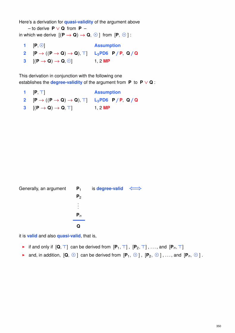
Here’s a derivation for quasi-validity of the argument above– to derive P ∨ Q from P –

in which we derive [(P→ Q)→ Q, � ] from [P, � ] :

1 [P,�] Assumption

2 [P→ ((P→ Q)→ Q),>] L3PD6 P//P, Q//Q

3 [(P→ Q)→ Q,�] 1, 2 MP

This derivation in conjunction with the following oneestablishes the degree-validity of the argument from P to P ∨ Q :

1 [P,>] Assumption

2 [P→ ((P→ Q)→ Q),>] L3PD6 P//P, Q//Q

3 [(P→ Q)→ Q,>] 1, 2 MP

Generally, an argument P1

P2

...

Pn

Q

is degree-valid ⇐⇒

it is valid and also quasi-valid, that is,

I if and only if [Q,>] can be derived from [P1,>] , [P2,>] , . . . , and [Pn,>]

I and, in addition, [Q, � ] can be derived from [P1, � ] , [P2, � ] , . . . , and [Pn, � ] .

350

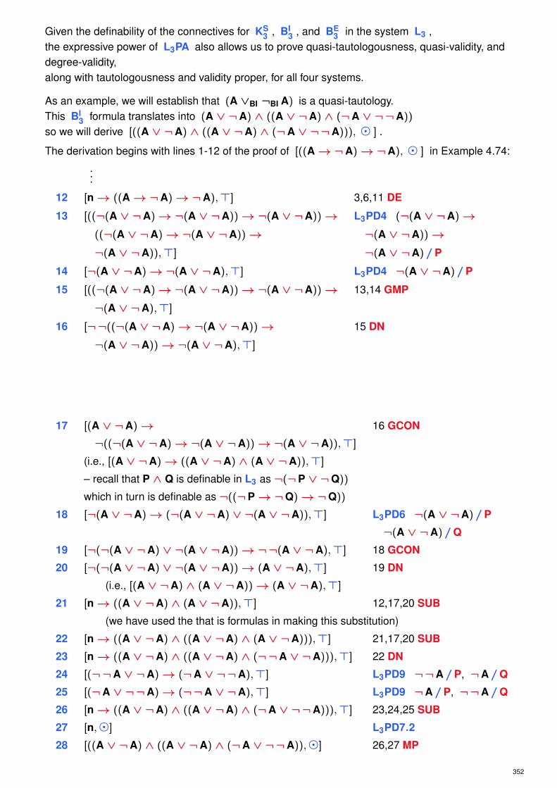
Given the definability of the connectives for KS3 , BI

3 , and BE3 in the system L3 ,

the expressive power of L3PA also allows us to prove quasi-tautologousness, quasi-validity, anddegree-validity,along with tautologousness and validity proper, for all four systems.

As an example, we will establish that (A ∨BI ¬BI A) is a quasi-tautology.This BI

3 formula translates into (A ∨ ¬A) ∧ ((A ∨ ¬A) ∧ (¬A ∨ ¬¬A))

so we will derive [((A ∨ ¬A) ∧ ((A ∨ ¬A) ∧ (¬A ∨ ¬¬A))), � ] .

The derivation begins with lines 1-12 of the proof of [((A→¬A)→¬A), � ] in Example 4.74:

...

12 [n→ ((A→¬A)→¬A),>] 3,6,11 DE

13 [((¬(A ∨ ¬A)→¬(A ∨ ¬A))→¬(A ∨ ¬A))→ L3PD4 (¬(A ∨ ¬A)→((¬(A ∨ ¬A)→¬(A ∨ ¬A))→ ¬(A ∨ ¬A))→¬(A ∨ ¬A)),>] ¬(A ∨ ¬A)//P

14 [¬(A ∨ ¬A)→¬(A ∨ ¬A),>] L3PD4 ¬(A ∨ ¬A)//P

15 [((¬(A ∨ ¬A)→¬(A ∨ ¬A))→¬(A ∨ ¬A))→ 13,14 GMP

¬(A ∨ ¬A),>]

16 [¬¬((¬(A ∨ ¬A)→¬(A ∨ ¬A))→ 15 DN

¬(A ∨ ¬A))→¬(A ∨ ¬A),>]

17 [(A ∨ ¬A)→ 16 GCON

¬((¬(A ∨ ¬A)→¬(A ∨ ¬A))→¬(A ∨ ¬A)),>]

(i.e., [(A ∨ ¬A)→ ((A ∨ ¬A) ∧ (A ∨ ¬A)),>]

– recall that P ∧ Q is definable in L3 as ¬(¬P ∨ ¬Q))

which in turn is definable as ¬((¬P→¬Q)→¬Q))

18 [¬(A ∨ ¬A)→ (¬(A ∨ ¬A) ∨ ¬(A ∨ ¬A)),>] L3PD6 ¬(A ∨ ¬A)//P

¬(A ∨ ¬A)//Q

19 [¬(¬(A ∨ ¬A) ∨ ¬(A ∨ ¬A))→¬¬(A ∨ ¬A),>] 18 GCON

20 [¬(¬(A ∨ ¬A) ∨ ¬(A ∨ ¬A))→ (A ∨ ¬A),>] 19 DN

(i.e., [(A ∨ ¬A) ∧ (A ∨ ¬A))→ (A ∨ ¬A),>]

21 [n→ ((A ∨ ¬A) ∧ (A ∨ ¬A)),>] 12,17,20 SUB

(we have used the that is formulas in making this substitution)

22 [n→ ((A ∨ ¬A) ∧ ((A ∨ ¬A) ∧ (A ∨ ¬A))),>] 21,17,20 SUB

23 [n→ ((A ∨ ¬A) ∧ ((A ∨ ¬A) ∧ (¬¬A ∨ ¬A))),>] 22 DN

24 [(¬¬A ∨ ¬A)→ (¬A ∨ ¬¬A),>] L3PD9 ¬¬A//P, ¬A//Q

25 [(¬A ∨ ¬¬A)→ (¬¬A ∨ ¬A),>] L3PD9 ¬A//P, ¬¬A//Q

26 [n→ ((A ∨ ¬A) ∧ ((A ∨ ¬A) ∧ (¬A ∨ ¬¬A))),>] 23,24,25 SUB

27 [n,�] L3PD7.2

28 [((A ∨ ¬A) ∧ ((A ∨ ¬A) ∧ (¬A ∨ ¬¬A)),�] 26,27 MP

352

So far we have applied rules derived in L3A only to formulas that are graded with > .

This restriction is inconvenient, so we will now introduce graded versions of derived rules.

CON. From [¬P→¬Q, v ] infer [Q→ P, v ]

1 [¬P→¬Q, v ] given

2 [(¬P→¬Q)→ (Q→ P),>] L3P 3

3 [Q→ P, v ] 1,2 MP

HS. From [P→ Q, v1] and [Q→ R, v2] infer [P→ R, v3]

where v3 is defined in terms of v1 and v2 as specified in the following table(identical to MP):

v1 v2 v3

> > >> � �

> ⊥ ⊥

v1 v2 v3

� > �� ⊥� ⊥ ⊥

v1 v2 v3

⊥ > ⊥⊥ � ⊥⊥ ⊥ ⊥

Proof:


2 [Q→ R, v2] given

3 [(P→ Q)→ ((Q→ R)→ (P→ R)),>] L3P 2

4 [(Q→ R)→ (P→ R), v1] 1,3 MP

5 [P→ R, v3] 2,4 MP

Note that the computation of v3 from v1 and v2 is symmetric.

354

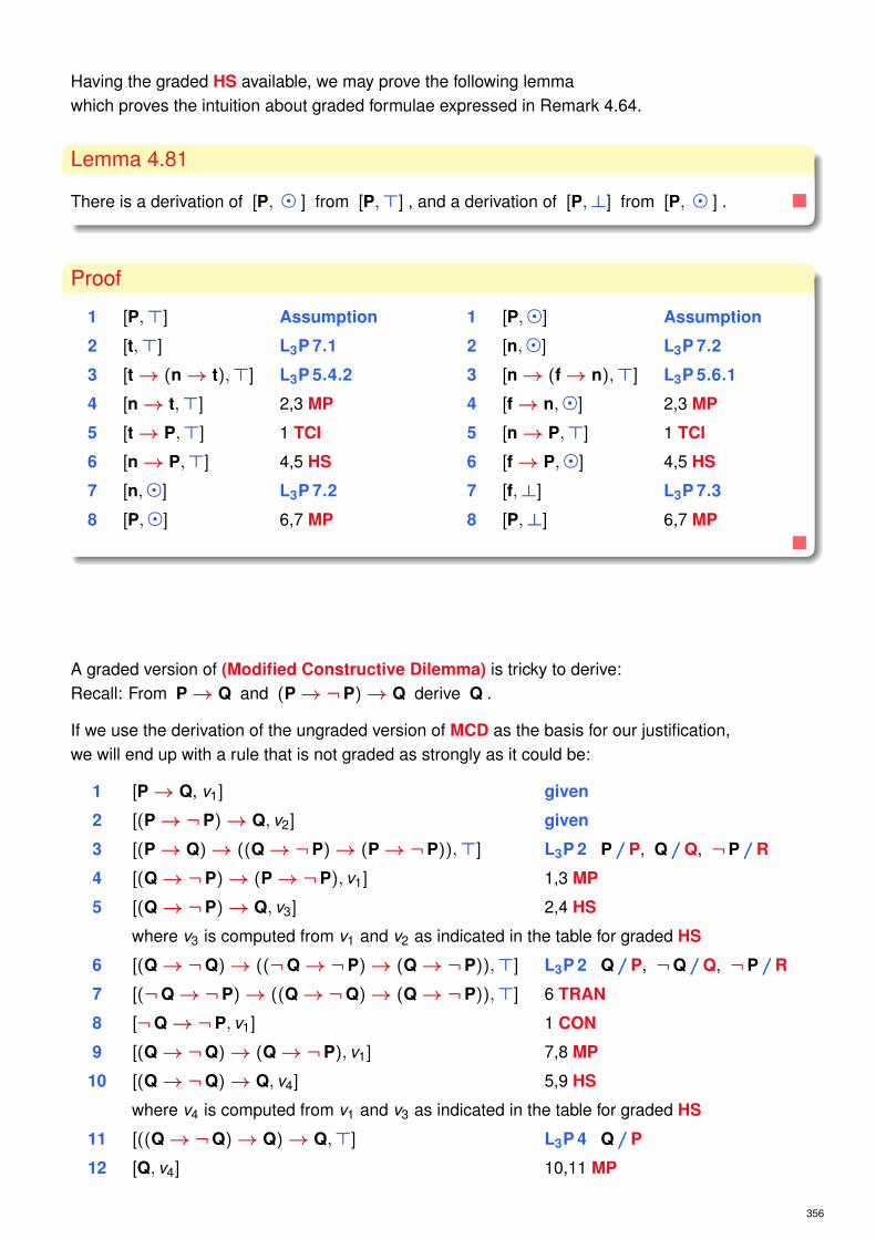
Having the graded HS available, we may prove the following lemmawhich proves the intuition about graded formulae expressed in Remark 4.64.

Lemma 4.81

There is a derivation of [P, � ] from [P,>] , and a derivation of [P,⊥] from [P, � ] .

Proof

1 [P,>] Assumption

2 [t,>] L3P 7.1

3 [t→ (n→ t),>] L3P 5.4.2

4 [n→ t,>] 2,3 MP

5 [t→ P,>] 1 TCI

6 [n→ P,>] 4,5 HS

7 [n,�] L3P 7.2

8 [P,�] 6,7 MP

1 [P,�] Assumption

2 [n,�] L3P 7.2

3 [n→ (f→ n),>] L3P 5.6.1

4 [f→ n,�] 2,3 MP

5 [n→ P,>] 1 TCI

6 [f→ P,�] 4,5 HS

7 [f,⊥] L3P 7.3

8 [P,⊥] 6,7 MP

A graded version of (Modified Constructive Dilemma) is tricky to derive:Recall: From P→ Q and (P→¬P)→ Q derive Q .

If we use the derivation of the ungraded version of MCD as the basis for our justification,we will end up with a rule that is not graded as strongly as it could be:


2 [(P→¬P)→ Q, v2] given

3 [(P→ Q)→ ((Q→¬P)→ (P→¬P)),>] L3P 2 P//P, Q//Q, ¬P//R

4 [(Q→¬P)→ (P→¬P), v1] 1,3 MP

5 [(Q→¬P)→ Q, v3] 2,4 HS

where v3 is computed from v1 and v2 as indicated in the table for graded HS

6 [(Q→¬Q)→ ((¬Q→¬P)→ (Q→¬P)),>] L3P 2 Q//P, ¬Q//Q, ¬P//R

7 [(¬Q→¬P)→ ((Q→¬Q)→ (Q→¬P)),>] 6 TRAN

8 [¬Q→¬P, v1] 1 CON

9 [(Q→¬Q)→ (Q→¬P), v1] 7,8 MP

10 [(Q→¬Q)→ Q, v4] 5,9 HS

where v4 is computed from v1 and v3 as indicated in the table for graded HS

11 [((Q→¬Q)→ Q)→ Q,>] L3P 4 Q//P

12 [Q, v4] 10,11 MP

356

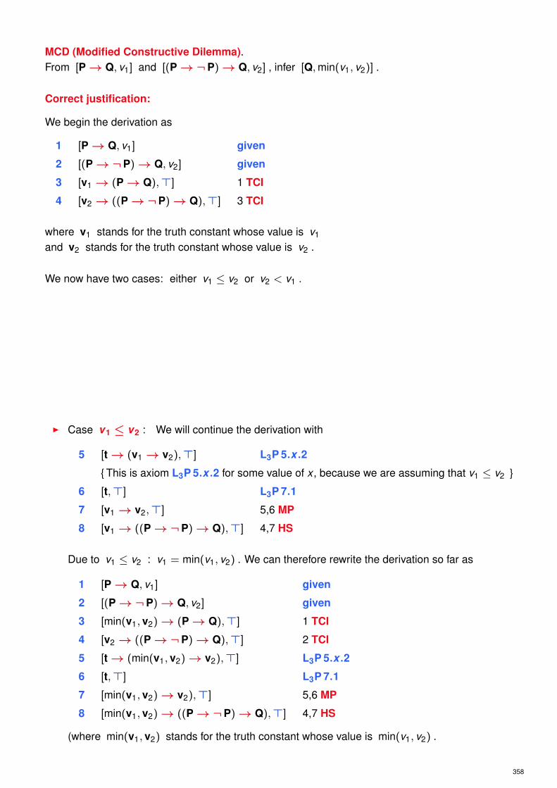
MCD (Modified Constructive Dilemma).From [P→ Q, v1] and [(P→¬P)→ Q, v2] , infer [Q,min(v1, v2)] .

Correct justification:

We begin the derivation as


2 [(P→¬P)→ Q, v2] given

3 [v1→ (P→ Q),>] 1 TCI

4 [v2→ ((P→¬P)→ Q),>] 3 TCI

where v1 stands for the truth constant whose value is v1

and v2 stands for the truth constant whose value is v2 .

We now have two cases: either v1 ≤ v2 or v2 < v1 .

I Case v1 ≤ v2 : We will continue the derivation with

5 [t→ (v1→ v2),>] L3P 5.x.2

{ This is axiom L3P 5.x.2 for some value of x , because we are assuming that v1 ≤ v2 }

6 [t,>] L3P 7.1

7 [v1→ v2,>] 5,6 MP

8 [v1→ ((P→¬P)→ Q),>] 4,7 HS

Due to v1 ≤ v2 : v1 = min(v1, v2) . We can therefore rewrite the derivation so far as


2 [(P→¬P)→ Q, v2] given

3 [min(v1, v2)→ (P→ Q),>] 1 TCI

4 [v2→ ((P→¬P)→ Q),>] 2 TCI

5 [t→ (min(v1, v2)→ v2),>] L3P 5.x.2

6 [t,>] L3P 7.1

7 [min(v1, v2)→ v2),>] 5,6 MP

8 [min(v1, v2)→ ((P→¬P)→ Q),>] 4,7 HS

(where min(v1, v2) stands for the truth constant whose value is min(v1, v2) .

358

I Case v2 < v1 : We begin the derivation with


2 [(P→¬P)→ Q, v2] given

3 [v1→ (P→ Q),>] 1 TCI

4 [min(v1, v2)→ ((P→¬P)→ Q),>] 2 TCI

5 [t→ (min(v1, v2)→ v1),>] L3P 5.x.2

6 [t,>] L3P 7.1

7 [min(v1, v2)→ v1),>] 5,6 MP

8 [min(v1, v2)→ (P→ Q),>] 3,7 HS

In either of the two cases above the derivation continues as follows(with { x , y } meaning line x if we began the first way, and line y if we began the second way):

9 [(P→ (min(v1, v2)→ Q),>] { 3,8 } TRAN

10 [(P→¬P)→ (min(v1, v2)→ Q),>] { 8,4 } TRAN

11 [(P→ (min(v1, v2)→ Q))→ L3P 2 P//P,

(((min(v1, v2)→ Q)→¬P)→ (P→¬P)),>] min(v1, v2)→ Q//Q

¬P//R

12 [((min(v1, v2)→ Q)→¬P)→ (P→¬P),>] 9,11 MP

13 [((min(v1, v2)→ Q)→¬P)→ (min(v1, v2)→ Q),>] 10,12 HS

14 [((min(v1, v2)→ Q)→¬(min(v1, v2)→ Q))→ L32 min(v1, v2)→ Q//P,

((¬(min(v1, v2)→ Q)→¬P)→ ¬(min(v1, v2)→ Q)//Q

((min(v1, v2)→ Q)→¬P)),>] ¬P//R

15 [(¬(min(v1, v2)→ Q)→¬P)→ 14 TRAN

(((min(v1, v2)→ Q)→¬(min(v1, v2)→ Q))→((min(v1, v2)→ Q)→¬P)),>]

360

16 [¬(min(v1, v2)→ Q)→¬P,>] 9 CON

17 [((min(v1, v2)→ Q)→¬(min(v1, v2)→ Q))→ 15,16 MP

((min(v1, v2)→ Q)→¬P),>]

18 [((min(v1, v2)→ Q)→¬(min(v1, v2)→ Q))→ 13,17 HS

(min(v1, v2)→ Q),>]

19 [(((min(v1, v2)→ Q)→¬(min(v1, v2)→ Q))→ L3P 4 min(v1, v2)→ Q//P

(min(v1, v2)→ Q))→ (min(v1, v2)→ Q),>]

20 [(min(v1, v2)→ Q),>] 18,19 MP

21 [min(v1, v2),min(v1, v2)] L3P 7.x

22 [Q,min(v1, v2)] 20,21 MP

Example 4.82Thus, for example, we can derive [P ∨ Q, � ] from [(P→¬P)→ (P ∨ Q), � ] as follows

1 [(P→¬P)→ (P ∨ Q),�] Assumption

2 [P→ (P ∨ Q),>] L3PD6 P//P, Q//Q

3 [P ∨ Q,�] 1,2 MCD

because � = min(>, � ) .

362

SUB (Substitution).From [P→ Q,>] , [Q→ P,>] ,and a graded formula [R, v ] such that R contains P as a subformula,infer any graded formula [R?, v ]

in which R? is the result of replacing one or more occurrences of P in R with Q .

With v the truth constant with value v , we get:

1 [R, v ] given

2 [P→ Q,>] given

3 [Q→ P,>] given

4 [v→ R,>] 1 TCI

5 [v→ R?,>] 2,3,4 SUB

6 [R?, v ] 5 CTCI

Lemma 4.83If P is at least � , then ¬P is at most � , i.e., from [P, � ] follows [¬P→ n,>] .

1 [P,�] given

2 [n→ P,>] 1 TCI

3 [¬P→¬n,>] 2 CON

4 [n→¬n,>] L3P 6.2.2

5 [¬n→ n,>] L3P 6.2.1

6 [¬P→ n,>] 3,4,5 SUB

364

Can we build a Pavelka-Style system for Kleene’s strong 3-valued logic?

The answer is negative.

Remark 4.84

Reconsider the formulae of Remark 4.62, but now as formulae of KS3

I t P t→K P

T T T

T � �T ⊥ ⊥

n P n→K P

� T T

� � �

� ⊥ �

f P f→K P

⊥ T T

⊥ � T

⊥ ⊥ T

I t P P→K t

T T T

T � T

T ⊥ T

n P P→K n

� T ��

� ⊥ T

f P P→K f

⊥ T ⊥⊥ � �⊥ ⊥ T

Basic Idea ‘a formula P is of value v ’ should be equivalent to ‘ v→ P and P→ v ’

This means that if P is neutral, then both n→K P and P→K n should hold.However, with KS

3 neither holds.

P n→K P

T T

� �⊥ �

P n→ P

T T

� T

⊥ �

P P→K n

T �� ⊥ T

P P→ n

T �� T

⊥ T

Special Case P = n

What we want is that [n→K n,>] and [n, � ] are equivalent.However, this does not hold for Kleene’s KS

3

Or again in different words

What we want is that n→K n is true,But this is just the difference between Kleene and Łukasiewicz

366

Now the other way round:

I If [P→ n, � ]

– ‘if P→ n is at most neutral’ is at least neutral –

then [n→ (P→ n),>] should hold ( and holds in L3 due to L31 )(or we would need at least a unique conclusion)

I However, if [P→K n, � ] , then [n→K (P→K n),>] doesn’t follow,

P n → (P → n)

T � T T � �� T � T �⊥ � T ⊥ T �

P n →K (P →K n)

T � � T � �� ⊥ � T ⊥ T �

Or looking at: v↔ P

P v v ↔K P

T T T T T

T � � � T

T ⊥ ⊥ ⊥ T

� T T � �� ⊥ ⊥ � �⊥ T T ⊥ ⊥⊥ � � � ⊥⊥ ⊥ ⊥ T ⊥

We cannot see that v↔K P will mean: P has exactly the truth-value v .

In contrast to v↔ P !

368

With Bochvar’s connectives it doesn’t work neither

P P→BI n

T �� ⊥ �

P P→BE n

T ⊥� T

⊥ T

P n→BI P

T �� ⊥ �

P n→BE P

T T

� T

⊥ T

5. Łukasiewicz Modalities

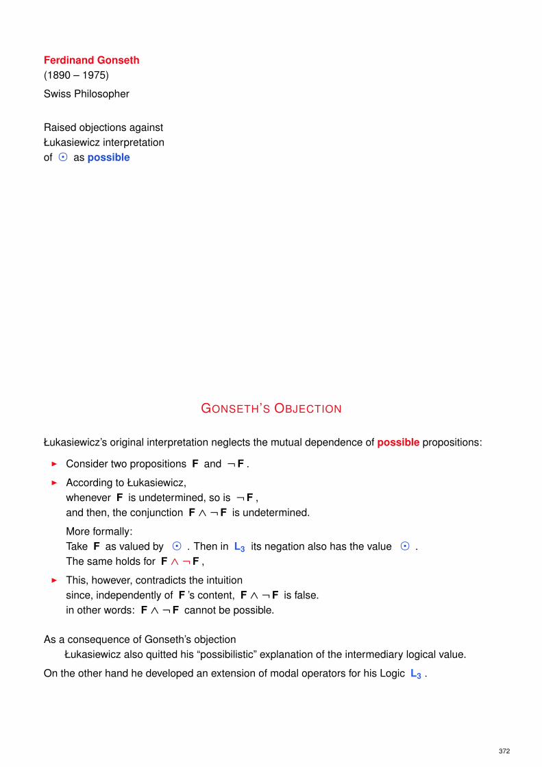
Ferdinand Gonseth(1890 – 1975)

Swiss Philosopher

Raised objections againstŁukasiewicz interpretationof � as possible

GONSETH’S OBJECTION

Łukasiewicz’s original interpretation neglects the mutual dependence of possible propositions:

I Consider two propositions F and ¬F .

I According to Łukasiewicz,whenever F is undetermined, so is ¬F ,and then, the conjunction F ∧ ¬F is undetermined.

More formally:Take F as valued by � . Then in L3 its negation also has the value � .The same holds for F ∧ ¬F ,

I This, however, contradicts the intuitionsince, independently of F ’s content, F ∧ ¬F is false.in other words: F ∧ ¬F cannot be possible.

As a consequence of Gonseth’s objectionŁukasiewicz also quitted his “possibilistic” explanation of the intermediary logical value.

On the other hand he developed an extension of modal operators for his Logic L3 .

372

ŁUKASIEWICZ’S MODALITIES

I Intention: to formalize the modal functors of possibility 3 and necessity 2 .Łukasiewicz attempted preservation of the consistency of middle ages intuitive theorems onmodal propositions.

I Being aware of the impossibility of classical logic for this purpose Łukasiewicz took the3-valued logic as base. (see next slides)

I Proposal: Modal operator 3 (as a unary connective) with intended meaning:

3 x = it is possible that x (where x is a propositional formula)

I Consequently we get the following readings:

• ¬ 3 x it is impossible that x

• 3 ¬x it is possible that x is not

• ¬ 3 ¬x it is impossible that x is not (= it is necessary that x)

I Moreover the following axioms are originally assumed

1. ¬ 3 x → ¬x what is not possible, that cannot be

2. ¬x → ¬ 3 x what is not, that cannot be possible

3. There is an x such that : 3 x ∧ 3 ¬x

CLASSICAL SEMANTICAL CONTRADICTION

As a unary connective the connective3 would need to have as meaning one of the unary truth functions

¬? =? ⊥? >?

T ⊥ T ⊥ T

⊥ T ⊥ ⊥ T

But none of these functions satisfied the axioms given above:

ProofThe 1. and 2. axioms are only valid if 3 is the unary identity mapping =? on truth values.

However, this is refuted by the 3. axiom.

Recall: 1. ¬ 3 x → ¬x what is not possible, that cannot be

2. ¬x → ¬ 3 x what is not, that cannot be possible

3. There is an x such that : 3 x ∧ 3 ¬x

374

CLASSICAL SYNTACTIC CONTRADICTION

We derive from the second axiom:

3 x → x

and by substitution we get:

3 ¬x → ¬x

With the third axiom we now derive with MP that for an x with both 3 x and 3 ¬x holds:

3 x → x

3 x

x

and 3 ¬x → ¬x

3 ¬x

¬x

which is a contradiction in two-valued logic.

Remark 5.1Since 3-valued logic has more unary connectives,Łukasiewicz tied to escape these problems on the basis of L3 .

ŁUKASIEWICZ MODALITIES

For his definition of 3 Łukasiewicz finally required the following axioms:

1. ¬3P→¬P : what is not possible, that cannot be

2. ¬P→ (¬P→¬3P) : what is not, that cannot be possible

3. There is a P such that : 3P ∧ 3¬P

Consider the first Axiom (with X instead of 3P )

P X (¬ X) → (¬ P)

T T ⊥ T T ⊥ T

T � � � � ⊥ T

T ⊥ T ⊥ ⊥ ⊥ T

� T ⊥ T T � �� T � �� ⊥ T ⊥ � � �⊥ T ⊥ T T T ⊥⊥ � � � T T ⊥⊥ ⊥ T ⊥ T T ⊥

Consequences

(consider the blue columns,where the axiom is satisfied)

If P is true,then 3P must be true as well.

If P is neutral,then 3P must be either true or neutral.

376

Consider the second Axiom (with X instead of 3P )

P X (¬ P) → ((¬ P) → (¬ X))

T T ⊥ T T ⊥ T T ⊥ T

T � ⊥ T T ⊥ T T � �T ⊥ ⊥ T T ⊥ T T T ⊥� T � � T � � � ⊥ T

� � � � T � � T � �� ⊥ � � T � � T T ⊥⊥ T T ⊥ ⊥ T ⊥ ⊥ ⊥ T

⊥ � T ⊥ � T ⊥ � � �⊥ ⊥ T ⊥ T T ⊥ T T ⊥

Consequence If P is false, then 3P must be false as well.

Consider the third AxiomNeither a false not a true P can satisfy the 3rd axiom.A neutral P can satisfy the 3rd axiom only if 3P is true.

Conclusion The connective 3 is uniquely determined by the 3 axioms.

Alfred Tarski(1902 – 1983)

In 1921Tarski produced a simple definitionof modal operatorsin terms of Łukasiewicz’s connectives,which satisfy the axioms given above

378

Definition 5.2Tarski defined a possibility operator as follows

3P := ¬P→ P

and derived from that the following necessity operator

2P := ¬3¬P ( ≡ ¬(P→¬P) )

We get the following truth tables for the connectives 3 and 2

P 3P

T T

� T

⊥ ⊥

P 2P

T T

� ⊥⊥ ⊥

Concerning the ‘Original’ 2nd Axiom

Note: ¬P→¬3P doesn’t hold! P ¬ P → ¬ 3 P

T ⊥ T T ⊥ T T

� � � � ⊥ T �⊥ T ⊥ T T ⊥ ⊥

Trying to solve the “logical” equation given by the formula above, we get:

P X (¬ P) → (¬ X)

T T ⊥ T T ⊥ T

T � ⊥ T T � �T ⊥ ⊥ T T T ⊥� T � � � ⊥ T

� � � � T � �� ⊥ � � T T ⊥⊥ T T ⊥ ⊥ ⊥ T

⊥ � T ⊥ � � �⊥ ⊥ T ⊥ T T ⊥

Consequences

I For P true,we get no constraint on 3P .

I If P is false,then 3P must be false as well.

I If P is neutral,then 3P must be either false orneutral.

However, neither of these two choices wouldsatisfy the third axiom.

380

Derivability of Łukasiewicz’s new Axioms:

1st axiom

1 P→ (¬P→ P) L31 P//P, ¬P//Q

2 ¬(¬P→ P)→¬P 1 GCON

3 ¬3P→¬P 2 Definition of 3

2nd axiom

1 (¬P→ P)→ (¬P→ P) L3D4 ¬P→ P//P

2 ¬P→ ((¬P→ P)→ P) 1 TRAN

3 ¬P→ (¬P→¬(¬P→ P)) 2 GCON

4 ¬P→ (¬P→¬3P) 3 Definition of 3

Note: This yields ¬3P from ¬P by applying MP twice.

3rd axiom

In a Pavelka-Style system we may express that P is �by the two formulae [n→ P,>] and [P→ n,>]

From these we may derive

1 [P→ n,>] Assumption

2 [¬n→¬P,>] 1 GCON

3 [¬n→ n,>] L3P 6.2.1

4 [n→¬P,>] 3,4 HS

5 [P→¬P,>] 1,4 MP

6 [¬¬P→¬P,>] 5 DN

7 [3¬P,>] Def 3

1 [n→ P,>] Assumption

2 [¬P→¬n,>] 1 GCON

3 [¬n→ n,>] L3P 6.2.1

4 [¬P→ n,>] 3,4 HS

5 [¬P→ P,>] 1,4 MP

6 [3P,>] Def 3

With a final application of CIthis yields [3P ∧ 3¬P,>] from [n→ P,>] and [P→ n,>]

382

Using 3 , 2 and other Łukasiewicz connectives we a get third modal connective

it is contingent that or, it is modally indifferent,

which distinguishes the intermediate logical value.

I P := 3P ∧ ¬2P P I P

T ⊥� T⊥ ⊥

Applying I allows the formulation within L3A ,of counterparts of the law of the excluded middle and the principle of contradiction:

P ∨ I P ∨ ¬P P P ∨ (I P ∨ ¬ P)

T T T ⊥ T ⊥ ⊥ T� � T T � T � �⊥ ⊥ T ⊥ ⊥ T T ⊥

¬(P ∧ ¬ I P ∧ ¬P) P ¬ (P ∧ (¬ I P ∧ ¬ P))

T T T ⊥ T ⊥ T ⊥ ⊥ T� T � ⊥ ⊥ T � ⊥ � �⊥ T ⊥ ⊥ T ⊥ ⊥ T T ⊥

THE FAILURE

Many, if not most, laws and properties known from modal logic hold for L3 modalities, e.g.

P→ 3P , 2P→ P , 2P→ 3P , . . .

However:

P Q (3 P ∧ 3 Q) → 3 (P ∧ Q)

T T T T T T T T T T T T

T � T T T T � T T T � �T ⊥ T T ⊥ ⊥ ⊥ T ⊥ T ⊥ ⊥� T T � T T T T T � � T

� � T � T T � T T � � �� ⊥ T � ⊥ ⊥ ⊥ T ⊥ � ⊥ ⊥⊥ T ⊥ ⊥ ⊥ T T T ⊥ ⊥ ⊥ T

⊥ � ⊥ ⊥ ⊥ T � T ⊥ ⊥ ⊥ �⊥ ⊥ ⊥ ⊥ ⊥ ⊥ ⊥ T ⊥ ⊥ ⊥ ⊥

384

BIBLIOGRAPHY I

[Bergmann, 1981] Bergmann, M. (1981).Dmitri Bochvar: On a three-valued calculus and its application to the analysis of the paradoxesof the classical extended functional calculus.History and Philosophy of Logic, 2, 87–112.

[Bochvar, 1937] Bochvar, D. (1937).Ob odnom trekhznachnom ischislenii i ego primenenii k analizu paradoksov klassicheskogorasshirennogo funkciona’nogo ischislenija.Matematicheskij Sbornik, 4(46), 287–308.Engl. translation: [Bergmann, 1981].

[Fisch & Turquette, 1966] Fisch, M. & Turquette, A. (1966).Peirce’s triadic logic.Transactions of the Charles S. Peirce Society, II(2), 71 – 85.

[Hájek, 1998] Hájek, P. (1998).Metamathematics of Fuzzy Logic.Dordrecht: Kluwer Academic Publishers.

[Hammer, 2010] Hammer, E. (2010).Peirce’s logic.In E. N. Zalta (Ed.), The Stanford Encyclopedia of Philosophy. Winter 2010 edition.

BIBLIOGRAPHY II

[Kleene, 1952] Kleene, S. C. (1952).Introduction to Metamathematics.New York: Van Nostrand.

[Łukasiewicz, 1920] Łukasiewicz, J. (1920).O logice trójwartosciowej.Ruch Filozoficzny, 5, 169–71.Engl. transl. On three-valued logic in [McCall, 1967, p.16-18].

[Łukasiewicz, 1930] Łukasiewicz, J. (1930).Philosophische Bemerkungen zu mehrwertigen Systemen des Aussagenkalküls.Comptes rendus des séances de la Societé des Sciences et des Lettres de Varsovie, Cl.iii, 23,51–77.Engl. transl. Philosophical Remarks on Many-Valued Systems of Propositional Logic in[McCall, 1967, 40-65].

[McCall, 1967] McCall, S., Ed. (1967).Polish Logic: 1920-1939.Oxford University Press.

[Priest, 1979] Priest, G. (1979).The logic of paradox.Journal of PhiIosophical Logic, 8, 219–241.

BIBLIOGRAPHY III

[Prior, 1953] Prior, A. N. (1953).Three-valued logic and future contingents.The Philosophical Quarterly, 3(13), 317–326.

[Rescher, 1969] Rescher, N. (1969).Many-valued Logic.McGraw-Hill.

[Rosser & Turquette, 1952] Rosser, B. & Turquette, A. (1952).Many-valued Logics.North-Holland.

[Rothenberg, 2005] Rothenberg, R. (2005).Łukasiewicz’s many-valued logic as a doxastic modal logic.Master’s thesis, Department of Philosophy, University of St Andrews.

[Słupecki, 1936] Słupecki, J. (1936).Der volle dreiwertige Aussagenkalkül.Comptes rendus des séances de la Societé des Sciences et des Lettres de Varsovie, Cl.iii, 29,9–11.Engl. transl. The full three-valued propositional calculus in [McCall, 1967, 335–337].

BIBLIOGRAPHY IV

[Wajsberg, 1931] Wajsberg, M. (1931).Aksjomatyzacja trójwartosciowego rachunku zdan.Comptes rendus des séances de la Societé des Sciences et des Lettres de Varsovie, Cl.iii, 24.Engl. transl. Axiomatization of the three-valued propositional calculus in [McCall, 1967,264–284].

Documents

Introduction to Many-Valued Logics - Technische Universit¤t Dresden